

Compact Muon Solenoid
LHC, CERN
| CMS-PAS-B2G-24-016 | ||
| Search for pair-produced vector-like top quarks decaying to Lorentz-boosted topquarks and scalar bosons in proton-proton collisions at $ \sqrt{s}= $ 13 TeV | ||
| CMS Collaboration | ||
| 2026-05-18 | ||
| Abstract: The first search for pair-produced vector-like top quarks, T, decaying to a new scalar boson $ \phi $ and a standard model (SM) top quark is presented. The search targets events containing a photon pair originating from the decay of one of the scalar bosons, accompanied by all-hadronic decays of the SM top quark pair. The analysis is optimized for boosted top quark signatures in which the decay products of the top quarks are reconstructed as large-radius jets. The search is based on proton-proton collision data at a center-of-mass energy of $ \sqrt{s}= $ 13 TeV, collected by the CMS experiment at the CERN LHC during 2016, 2017, and 2018, corresponding to an integrated luminosity of 138 fb$ ^{-1} $. The search is performed in the two-dimensional $ (m_{\mathrm{T}}, m_{\phi}) $ plane. No significant deviation from the standard model prediction is observed. Assuming a branching fraction of 100$ % $ for $ \phi \to \gamma\gamma $, upper limits at 95$ % $ confidence level are set on the $ \mathrm{T}\bar{\mathrm{T}} $ production cross section. Vector-like top quark masses below 1.39 TeV are excluded. | ||
| Links: CDS record (PDF) ; CADI line (restricted) ; | ||
| Figures | |
png pdf |
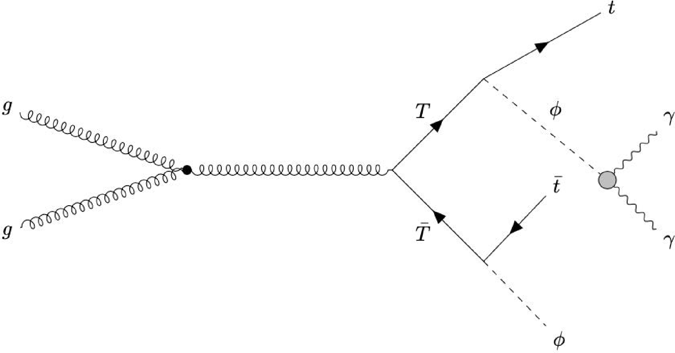
Figure 1:
A representative leading order Feynman diagram for the pair production of vector-like top quarks $ {\mathrm{T}} $ with subsequent $ {\mathrm{T}} \to \phi\mathrm{t} $ decays. |
png pdf |
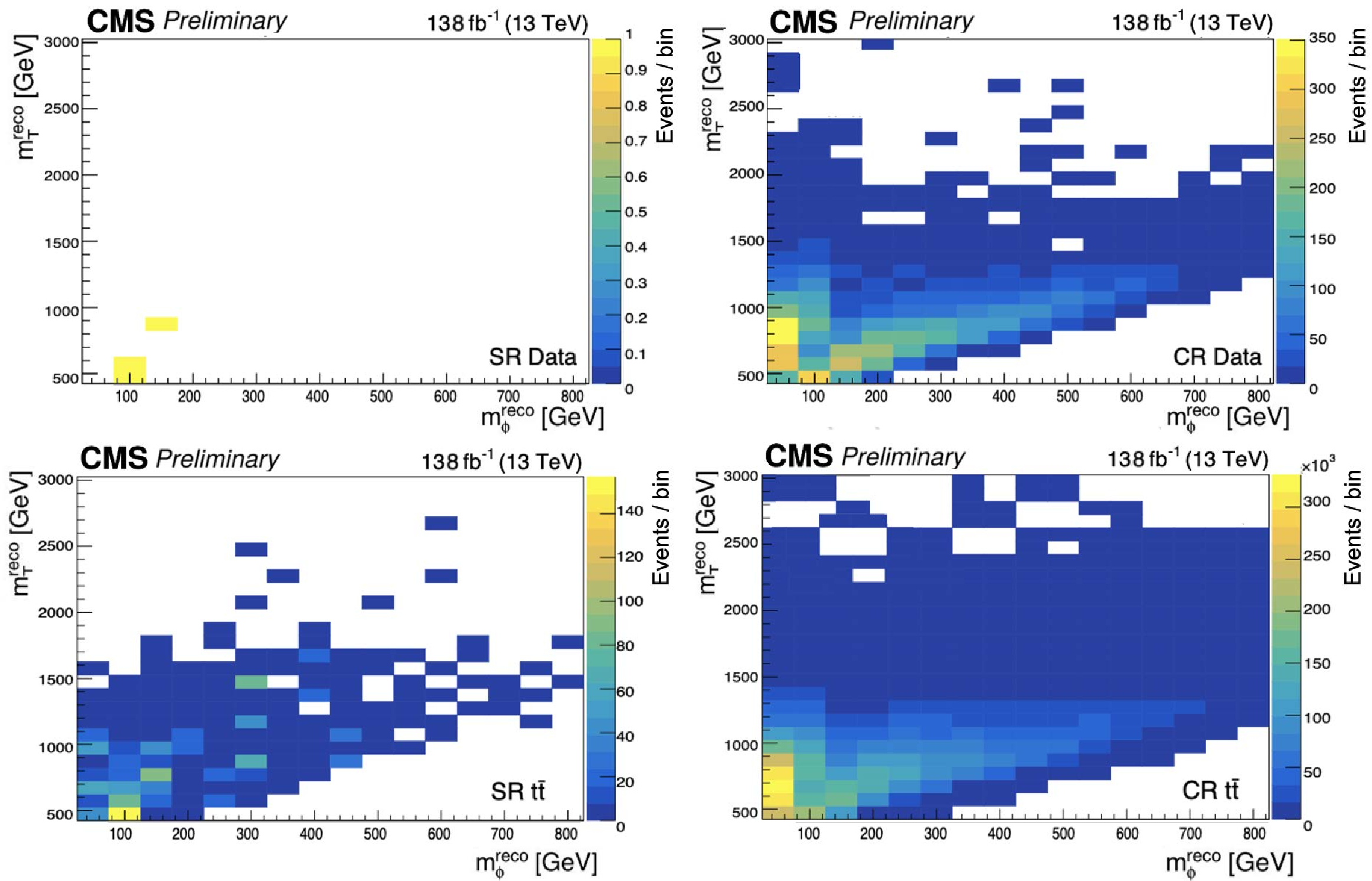
Figure 2:
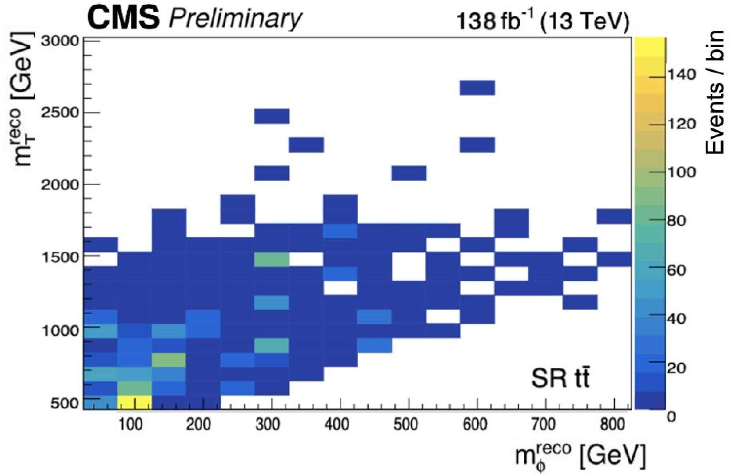
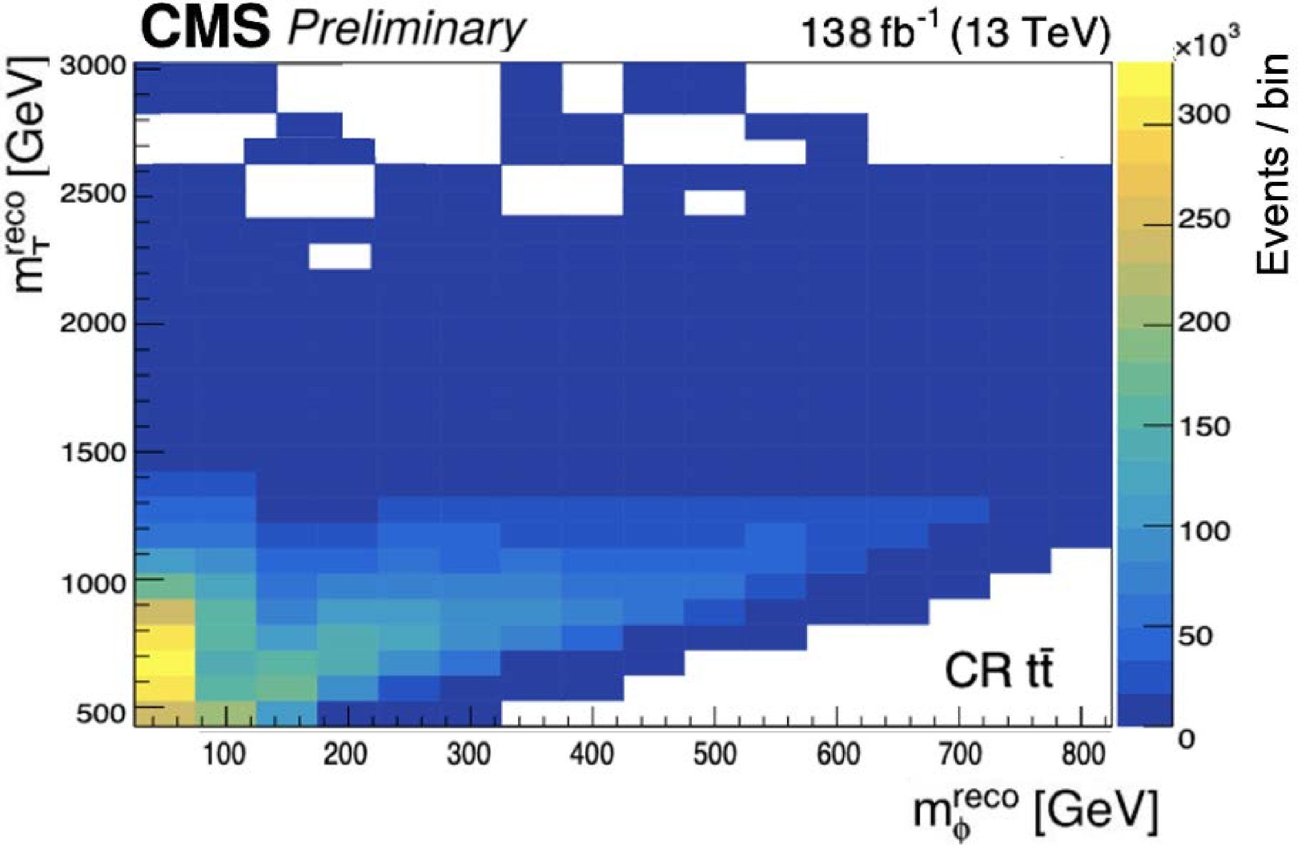
Distribution of reconstructed {\HepParticleT} candidates in the $ m^\mathrm{reco}_{{\mathrm{T}} } $--$ m^\mathrm{reco}_{\phi} $ plane for data (top) and simulated $ \mathrm{t}\overline{\mathrm{t}} $ events (bottom), shown for the SR (left) and CR (right). |
png pdf |
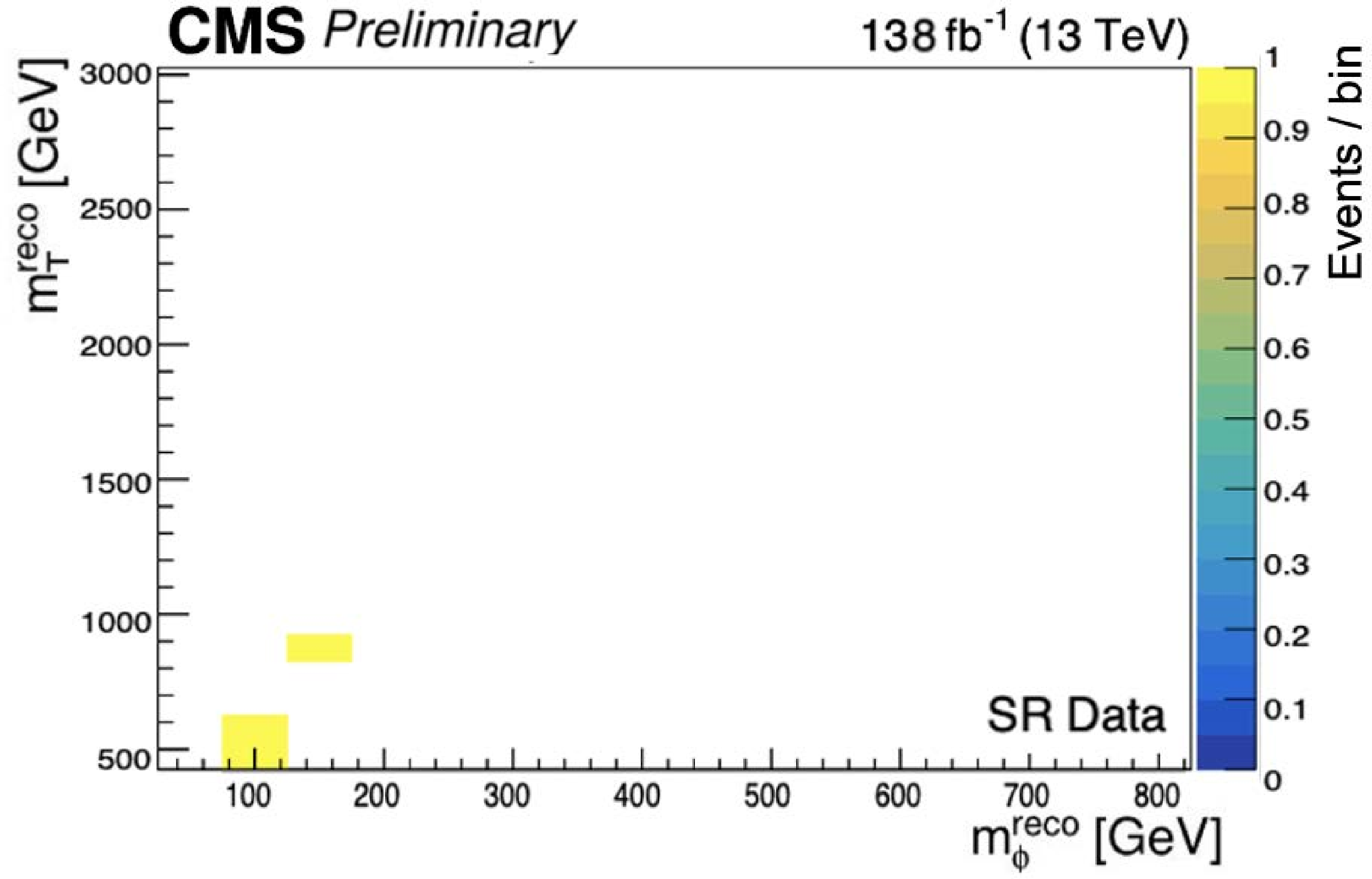
Figure 2-a:
Distribution of reconstructed {\HepParticleT} candidates in the $ m^\mathrm{reco}_{{\mathrm{T}} } $--$ m^\mathrm{reco}_{\phi} $ plane for data (top) and simulated $ \mathrm{t}\overline{\mathrm{t}} $ events (bottom), shown for the SR (left) and CR (right). |
png pdf |
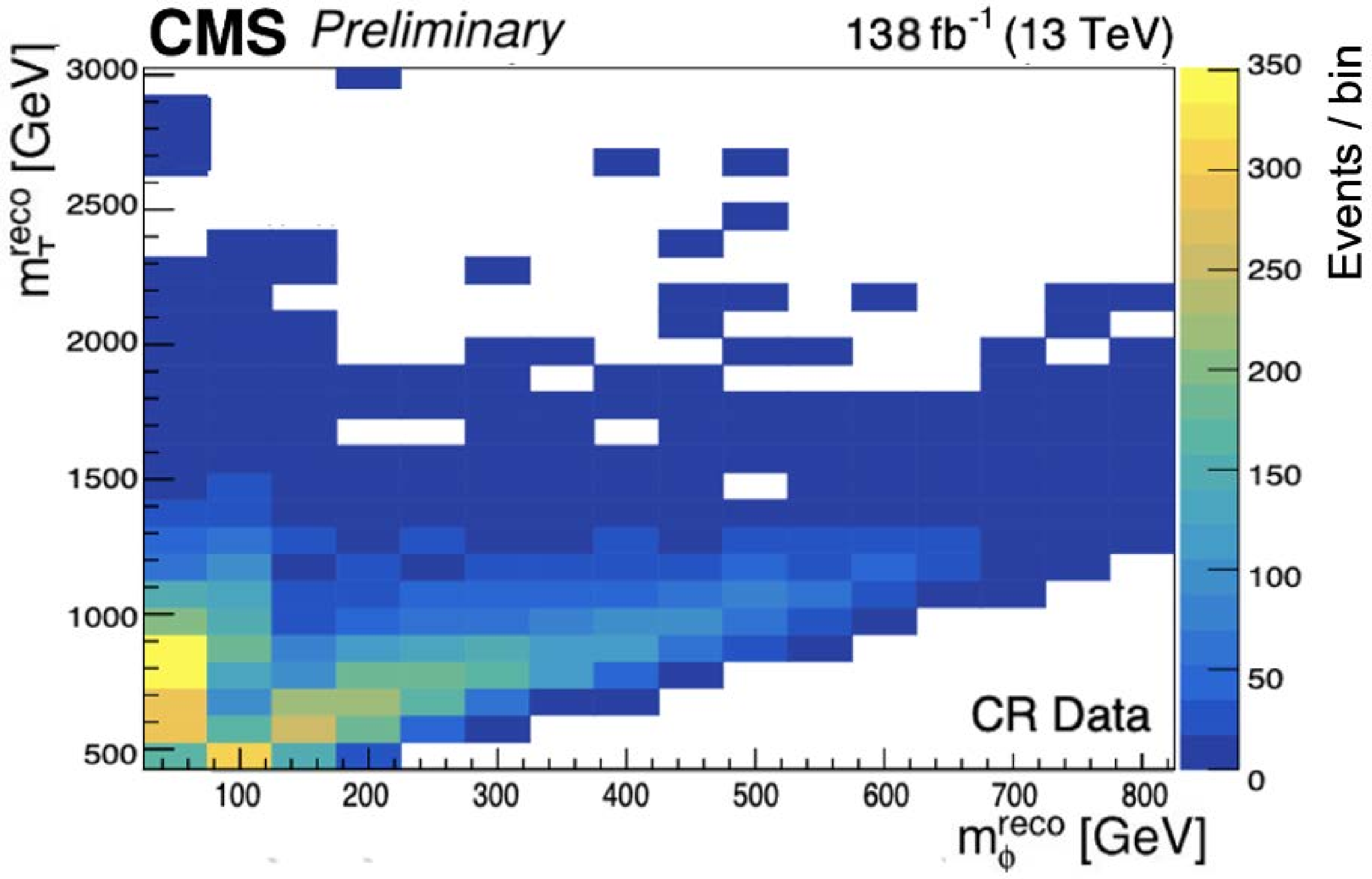
Figure 2-b:
Distribution of reconstructed {\HepParticleT} candidates in the $ m^\mathrm{reco}_{{\mathrm{T}} } $--$ m^\mathrm{reco}_{\phi} $ plane for data (top) and simulated $ \mathrm{t}\overline{\mathrm{t}} $ events (bottom), shown for the SR (left) and CR (right). |
png pdf |
Figure 2-c:
Distribution of reconstructed {\HepParticleT} candidates in the $ m^\mathrm{reco}_{{\mathrm{T}} } $--$ m^\mathrm{reco}_{\phi} $ plane for data (top) and simulated $ \mathrm{t}\overline{\mathrm{t}} $ events (bottom), shown for the SR (left) and CR (right). |
png pdf |
Figure 2-d:
Distribution of reconstructed {\HepParticleT} candidates in the $ m^\mathrm{reco}_{{\mathrm{T}} } $--$ m^\mathrm{reco}_{\phi} $ plane for data (top) and simulated $ \mathrm{t}\overline{\mathrm{t}} $ events (bottom), shown for the SR (left) and CR (right). |
png pdf |
Figure 3:
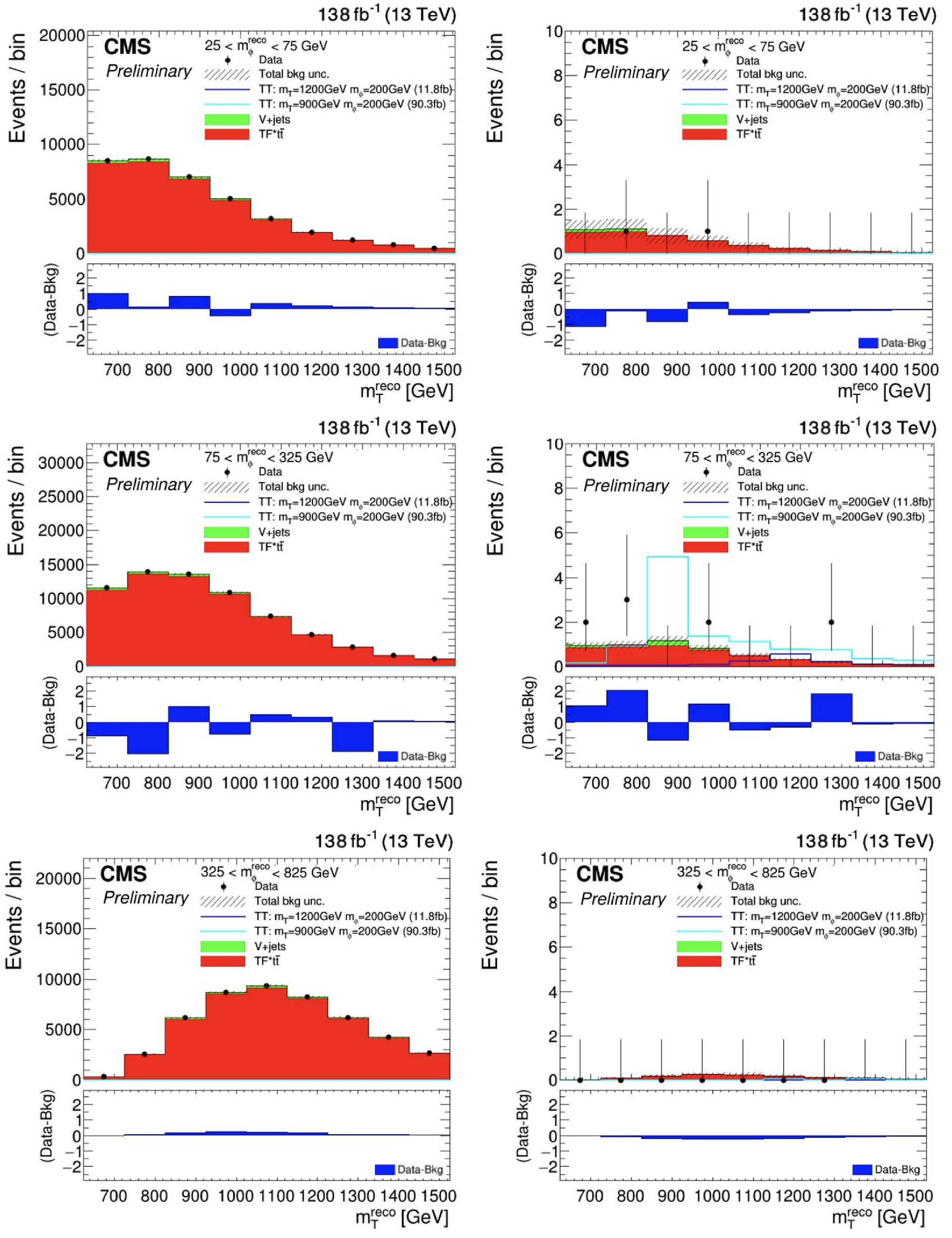
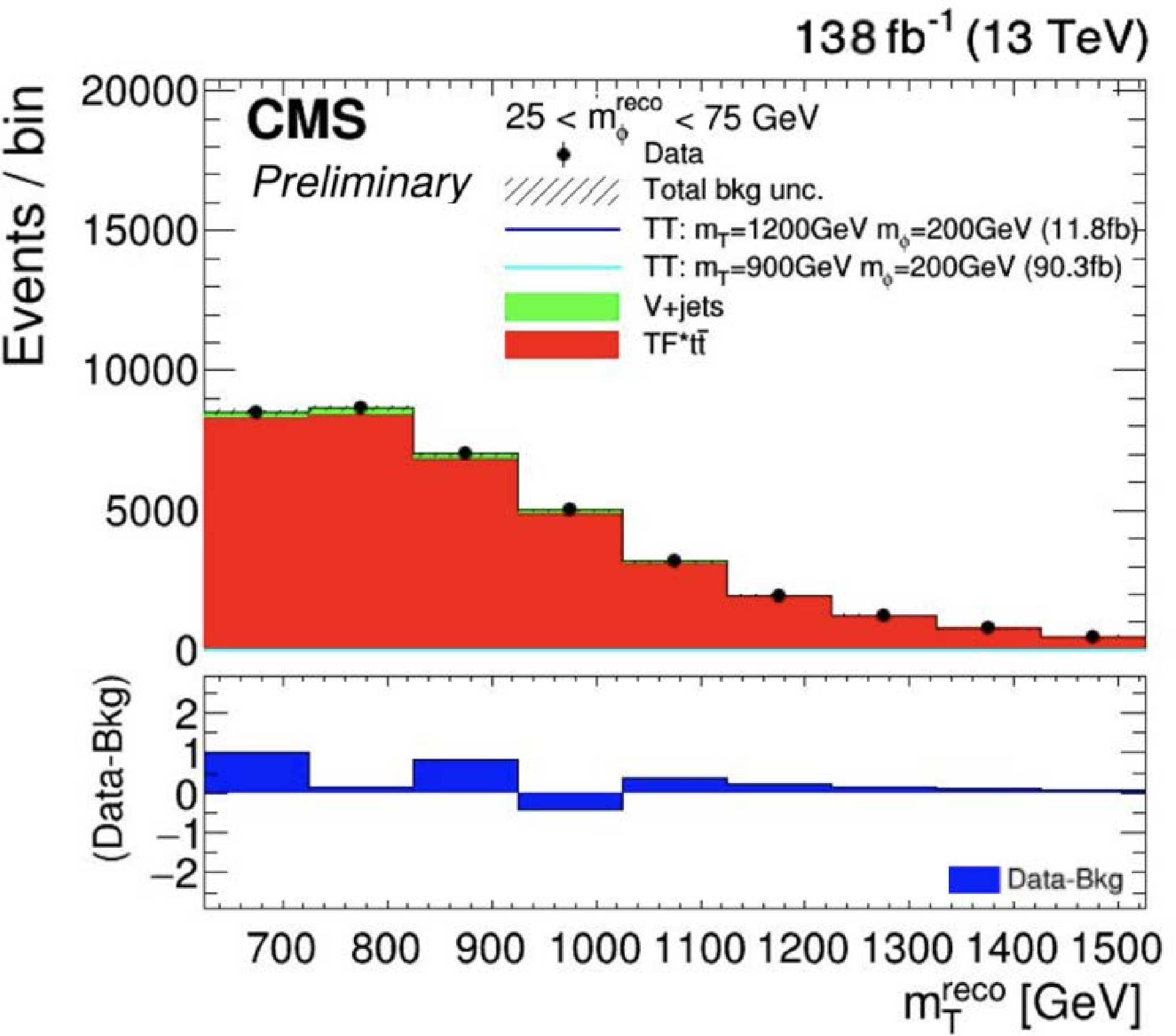
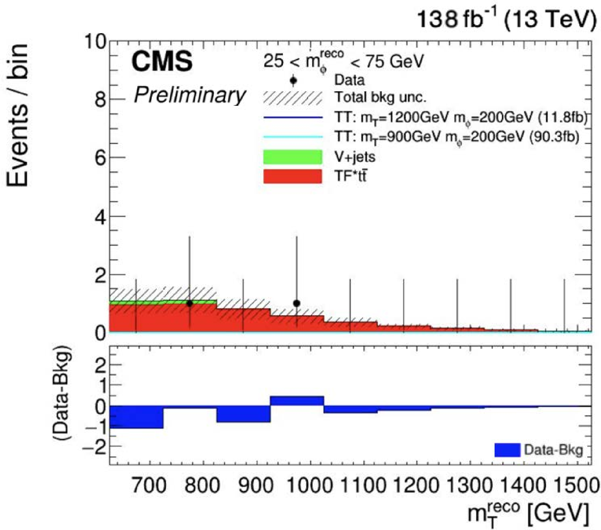
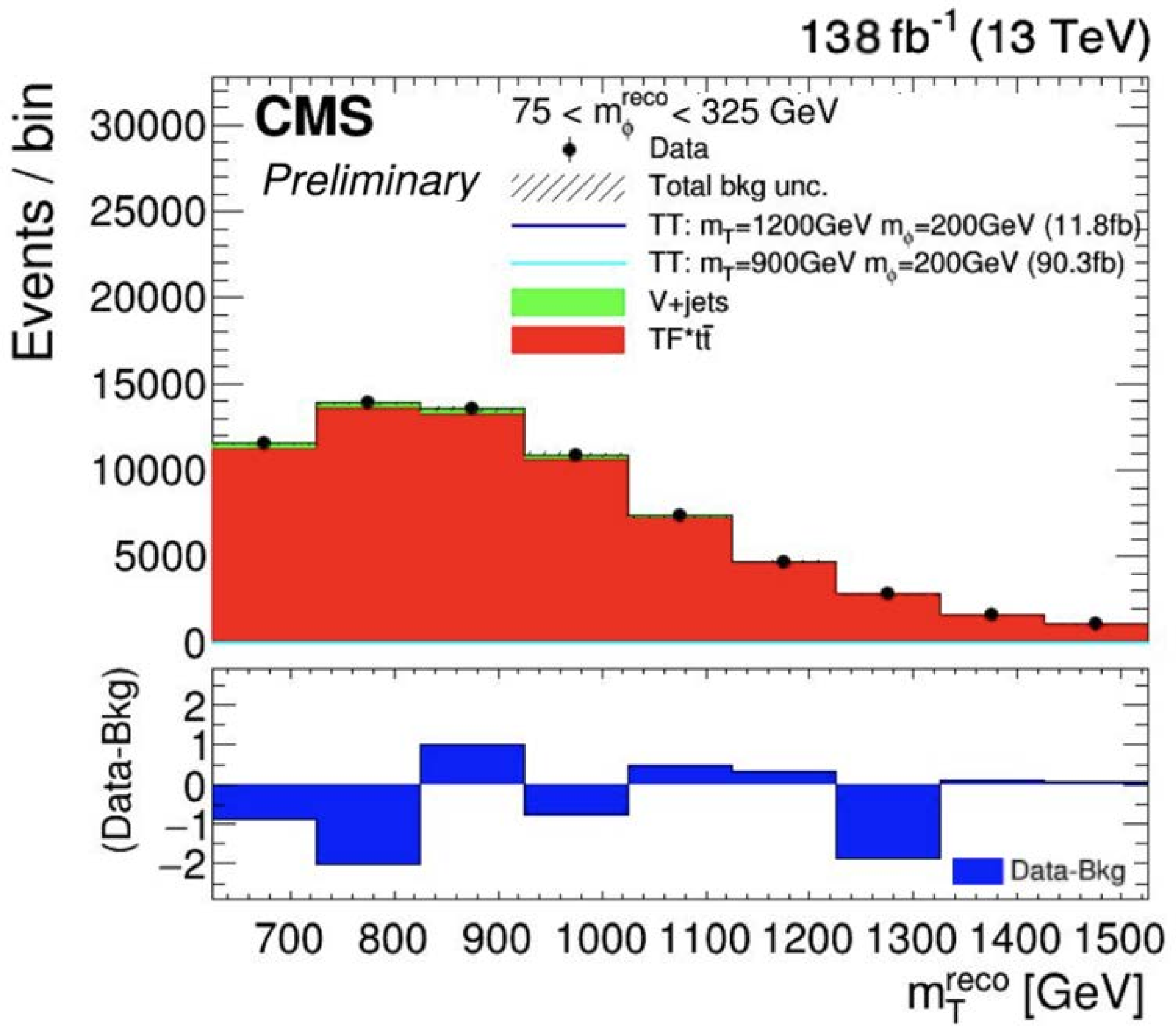
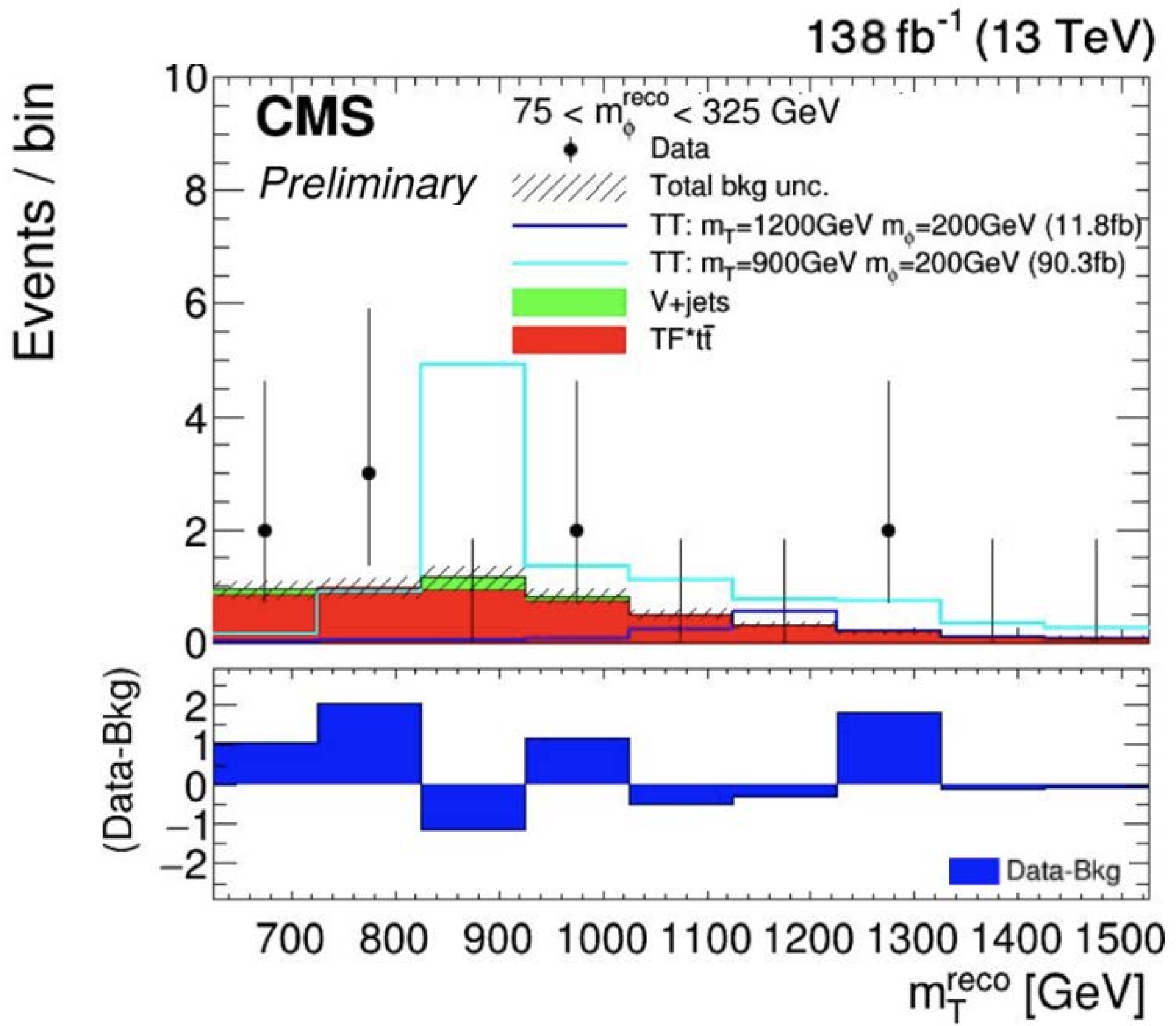
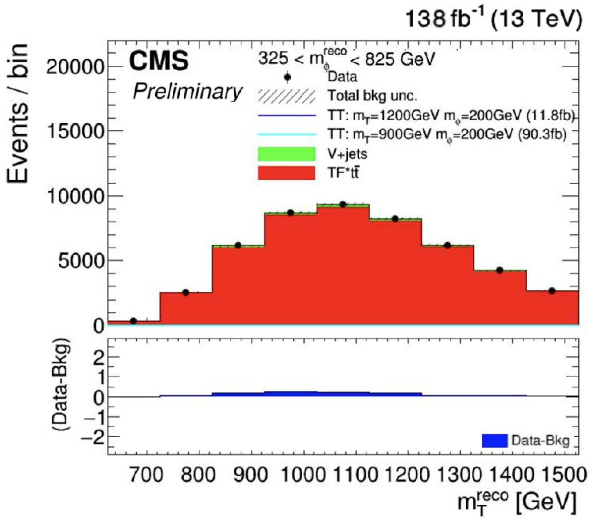
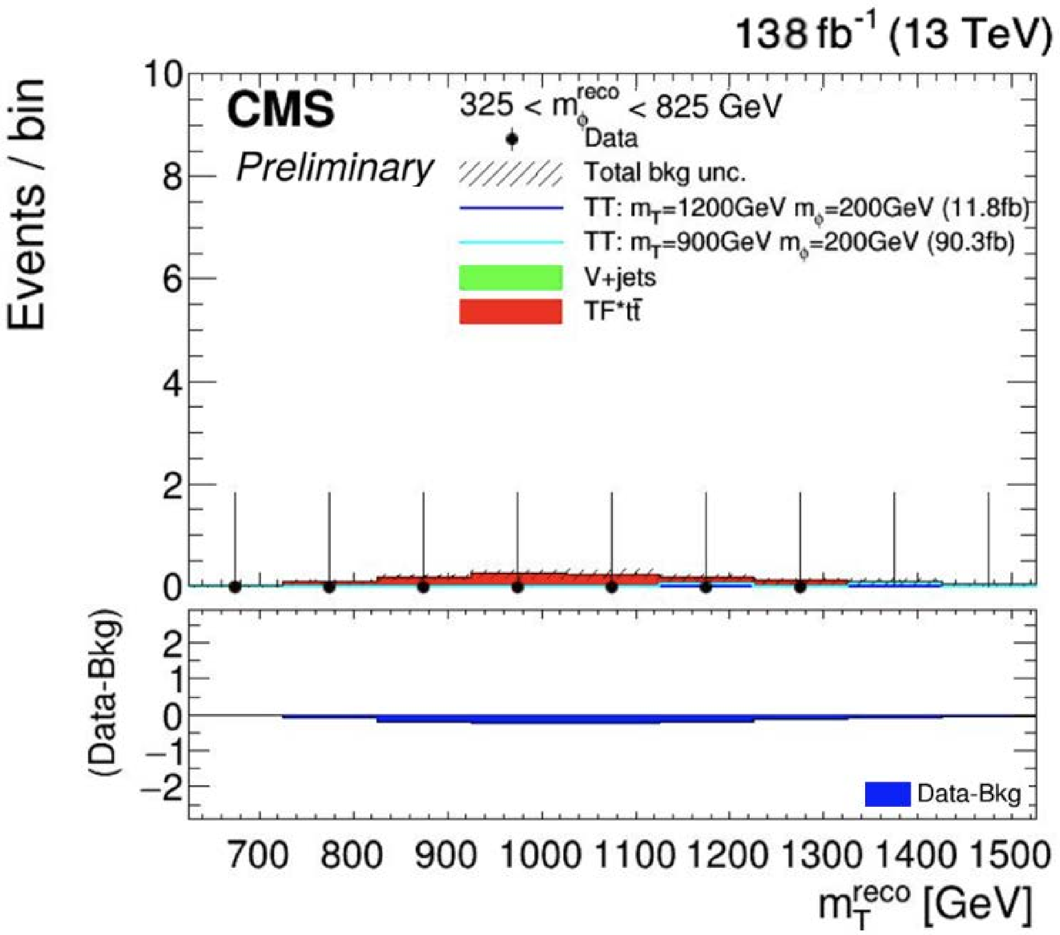
Comparison of data and the postfit background prediction from the background-only fit in the VR. The VR-CR (left) and VR-SR (right) regions are shown. The distributions are projected onto $ m^\mathrm{reco}_{{\mathrm{T}} } $ in three intervals of $ m^\mathrm{reco}_{\phi} $: 25 $ < m^\mathrm{reco}_{\phi} < $ 75 GeV (top), 75 $ < m^\mathrm{reco}_{\phi} < $ 325 GeV (middle), and 325 $ < m^\mathrm{reco}_{\phi} < $ 625 GeV (bottom). The $ \mathrm{t}\overline{\mathrm{t}} $ component scaled by the transfer function is shown in red and the $ \mathrm{W}/\mathrm{Z} $+jets contribution in green. Signal distributions for the mass hypotheses $ m_{{\mathrm{T}} }= $ 1200 GeV, $ m_{\phi}= $ 200 GeV and $ m_{{\mathrm{T}} }= $ 900 GeV, $ m_{\phi}= $ 100 GeV are overlaid as thin lines. The lower panels show the difference between the data and the background prediction. |
png pdf |
Figure 3-a:
Comparison of data and the postfit background prediction from the background-only fit in the VR. The VR-CR (left) and VR-SR (right) regions are shown. The distributions are projected onto $ m^\mathrm{reco}_{{\mathrm{T}} } $ in three intervals of $ m^\mathrm{reco}_{\phi} $: 25 $ < m^\mathrm{reco}_{\phi} < $ 75 GeV (top), 75 $ < m^\mathrm{reco}_{\phi} < $ 325 GeV (middle), and 325 $ < m^\mathrm{reco}_{\phi} < $ 625 GeV (bottom). The $ \mathrm{t}\overline{\mathrm{t}} $ component scaled by the transfer function is shown in red and the $ \mathrm{W}/\mathrm{Z} $+jets contribution in green. Signal distributions for the mass hypotheses $ m_{{\mathrm{T}} }= $ 1200 GeV, $ m_{\phi}= $ 200 GeV and $ m_{{\mathrm{T}} }= $ 900 GeV, $ m_{\phi}= $ 100 GeV are overlaid as thin lines. The lower panels show the difference between the data and the background prediction. |
png pdf |
Figure 3-b:
Comparison of data and the postfit background prediction from the background-only fit in the VR. The VR-CR (left) and VR-SR (right) regions are shown. The distributions are projected onto $ m^\mathrm{reco}_{{\mathrm{T}} } $ in three intervals of $ m^\mathrm{reco}_{\phi} $: 25 $ < m^\mathrm{reco}_{\phi} < $ 75 GeV (top), 75 $ < m^\mathrm{reco}_{\phi} < $ 325 GeV (middle), and 325 $ < m^\mathrm{reco}_{\phi} < $ 625 GeV (bottom). The $ \mathrm{t}\overline{\mathrm{t}} $ component scaled by the transfer function is shown in red and the $ \mathrm{W}/\mathrm{Z} $+jets contribution in green. Signal distributions for the mass hypotheses $ m_{{\mathrm{T}} }= $ 1200 GeV, $ m_{\phi}= $ 200 GeV and $ m_{{\mathrm{T}} }= $ 900 GeV, $ m_{\phi}= $ 100 GeV are overlaid as thin lines. The lower panels show the difference between the data and the background prediction. |
png pdf |
Figure 3-c:
Comparison of data and the postfit background prediction from the background-only fit in the VR. The VR-CR (left) and VR-SR (right) regions are shown. The distributions are projected onto $ m^\mathrm{reco}_{{\mathrm{T}} } $ in three intervals of $ m^\mathrm{reco}_{\phi} $: 25 $ < m^\mathrm{reco}_{\phi} < $ 75 GeV (top), 75 $ < m^\mathrm{reco}_{\phi} < $ 325 GeV (middle), and 325 $ < m^\mathrm{reco}_{\phi} < $ 625 GeV (bottom). The $ \mathrm{t}\overline{\mathrm{t}} $ component scaled by the transfer function is shown in red and the $ \mathrm{W}/\mathrm{Z} $+jets contribution in green. Signal distributions for the mass hypotheses $ m_{{\mathrm{T}} }= $ 1200 GeV, $ m_{\phi}= $ 200 GeV and $ m_{{\mathrm{T}} }= $ 900 GeV, $ m_{\phi}= $ 100 GeV are overlaid as thin lines. The lower panels show the difference between the data and the background prediction. |
png pdf |
Figure 3-d:
Comparison of data and the postfit background prediction from the background-only fit in the VR. The VR-CR (left) and VR-SR (right) regions are shown. The distributions are projected onto $ m^\mathrm{reco}_{{\mathrm{T}} } $ in three intervals of $ m^\mathrm{reco}_{\phi} $: 25 $ < m^\mathrm{reco}_{\phi} < $ 75 GeV (top), 75 $ < m^\mathrm{reco}_{\phi} < $ 325 GeV (middle), and 325 $ < m^\mathrm{reco}_{\phi} < $ 625 GeV (bottom). The $ \mathrm{t}\overline{\mathrm{t}} $ component scaled by the transfer function is shown in red and the $ \mathrm{W}/\mathrm{Z} $+jets contribution in green. Signal distributions for the mass hypotheses $ m_{{\mathrm{T}} }= $ 1200 GeV, $ m_{\phi}= $ 200 GeV and $ m_{{\mathrm{T}} }= $ 900 GeV, $ m_{\phi}= $ 100 GeV are overlaid as thin lines. The lower panels show the difference between the data and the background prediction. |
png pdf |
Figure 3-e:
Comparison of data and the postfit background prediction from the background-only fit in the VR. The VR-CR (left) and VR-SR (right) regions are shown. The distributions are projected onto $ m^\mathrm{reco}_{{\mathrm{T}} } $ in three intervals of $ m^\mathrm{reco}_{\phi} $: 25 $ < m^\mathrm{reco}_{\phi} < $ 75 GeV (top), 75 $ < m^\mathrm{reco}_{\phi} < $ 325 GeV (middle), and 325 $ < m^\mathrm{reco}_{\phi} < $ 625 GeV (bottom). The $ \mathrm{t}\overline{\mathrm{t}} $ component scaled by the transfer function is shown in red and the $ \mathrm{W}/\mathrm{Z} $+jets contribution in green. Signal distributions for the mass hypotheses $ m_{{\mathrm{T}} }= $ 1200 GeV, $ m_{\phi}= $ 200 GeV and $ m_{{\mathrm{T}} }= $ 900 GeV, $ m_{\phi}= $ 100 GeV are overlaid as thin lines. The lower panels show the difference between the data and the background prediction. |
png pdf |
Figure 3-f:
Comparison of data and the postfit background prediction from the background-only fit in the VR. The VR-CR (left) and VR-SR (right) regions are shown. The distributions are projected onto $ m^\mathrm{reco}_{{\mathrm{T}} } $ in three intervals of $ m^\mathrm{reco}_{\phi} $: 25 $ < m^\mathrm{reco}_{\phi} < $ 75 GeV (top), 75 $ < m^\mathrm{reco}_{\phi} < $ 325 GeV (middle), and 325 $ < m^\mathrm{reco}_{\phi} < $ 625 GeV (bottom). The $ \mathrm{t}\overline{\mathrm{t}} $ component scaled by the transfer function is shown in red and the $ \mathrm{W}/\mathrm{Z} $+jets contribution in green. Signal distributions for the mass hypotheses $ m_{{\mathrm{T}} }= $ 1200 GeV, $ m_{\phi}= $ 200 GeV and $ m_{{\mathrm{T}} }= $ 900 GeV, $ m_{\phi}= $ 100 GeV are overlaid as thin lines. The lower panels show the difference between the data and the background prediction. |
png pdf |
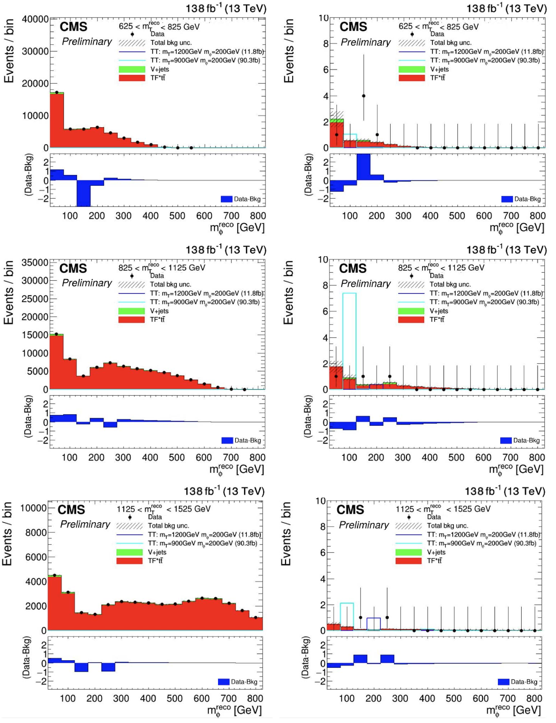
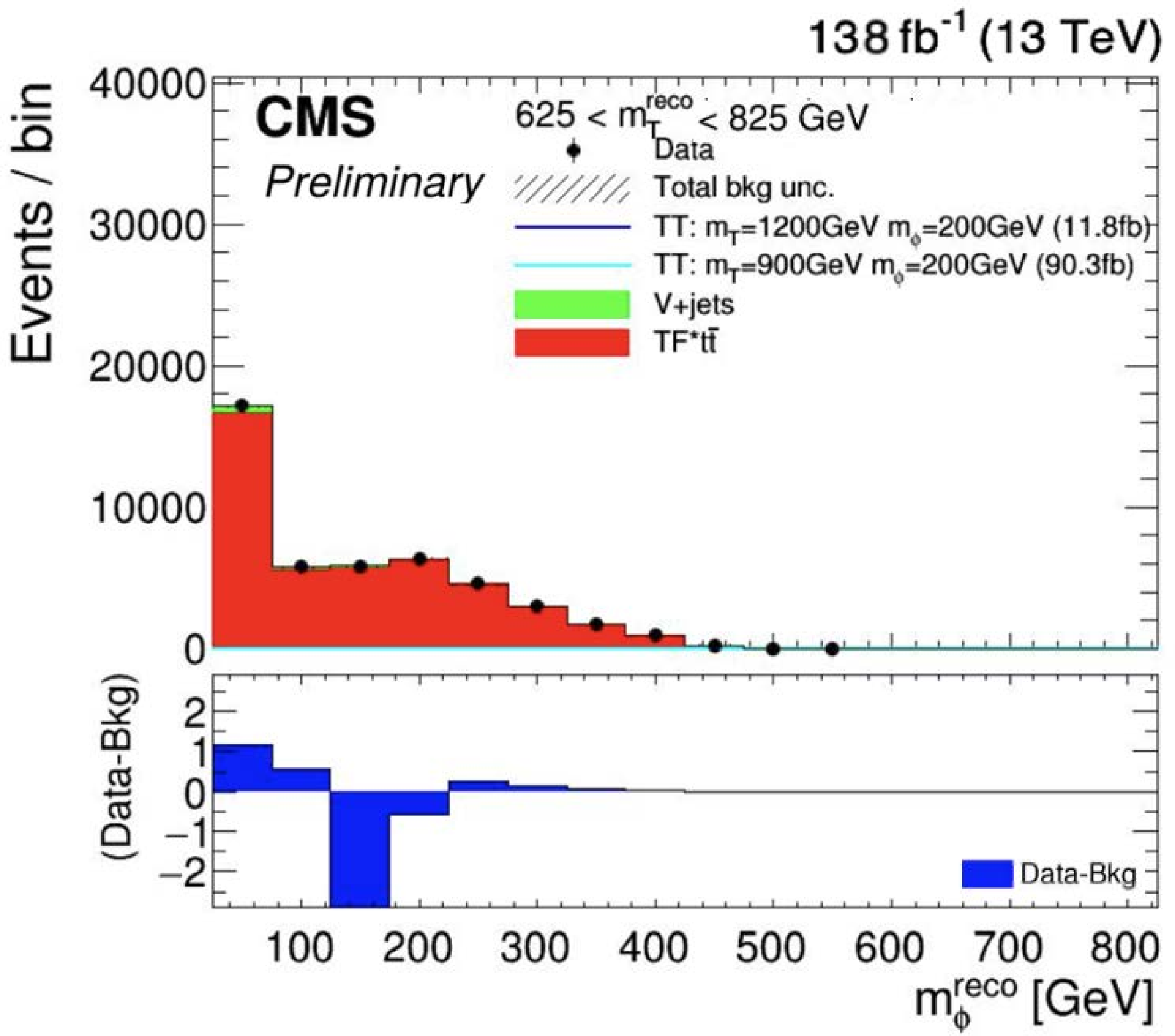
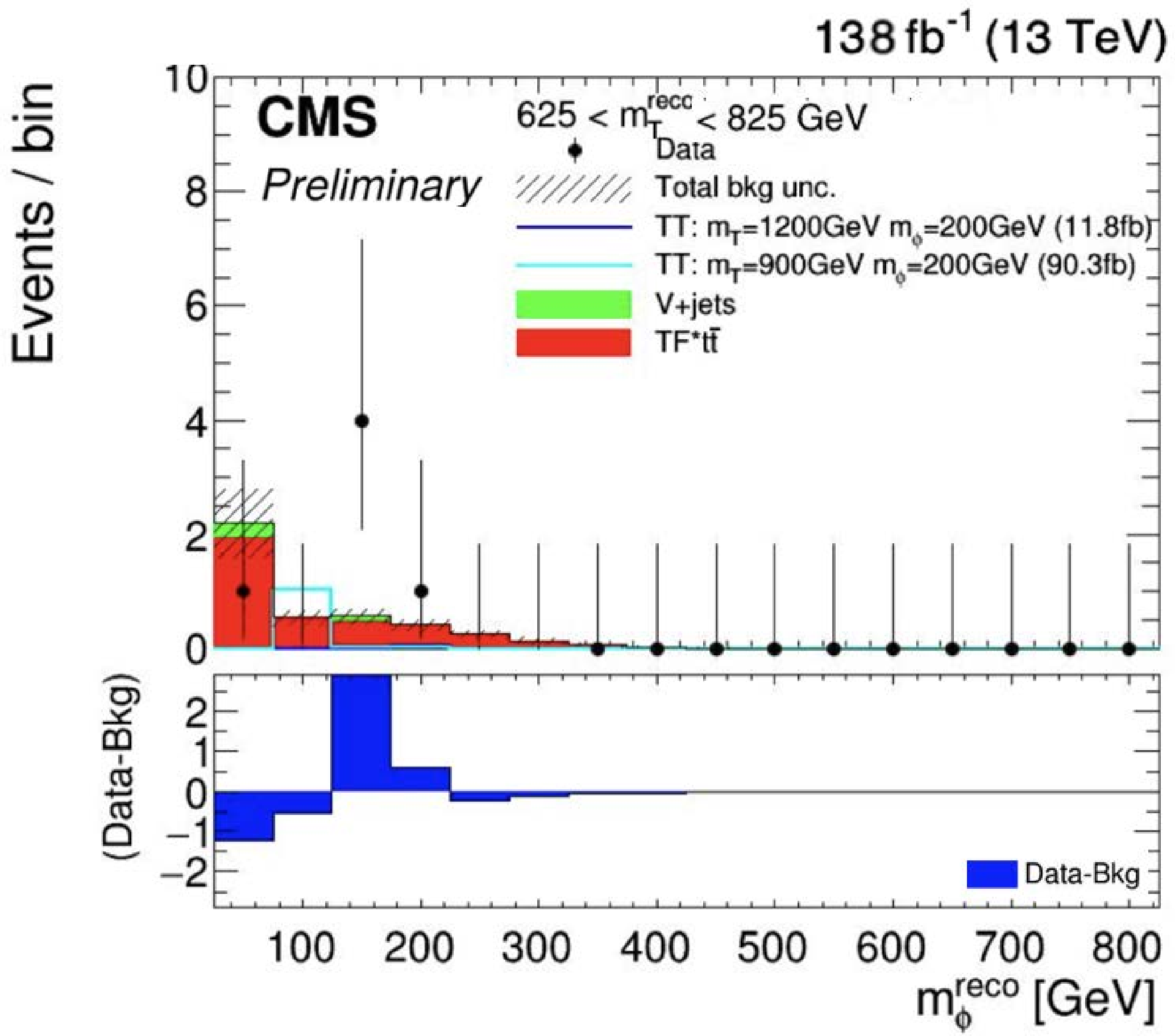
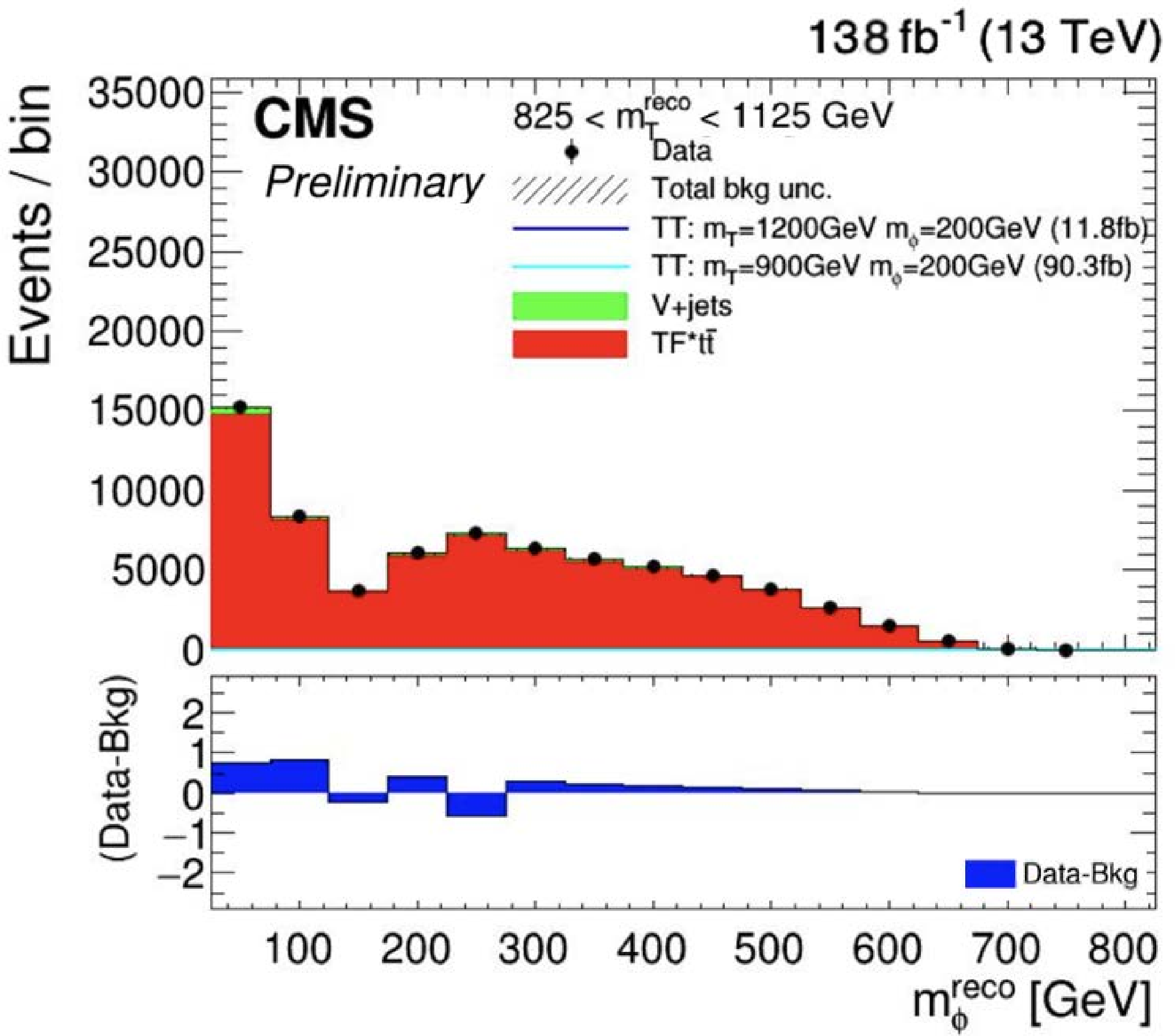
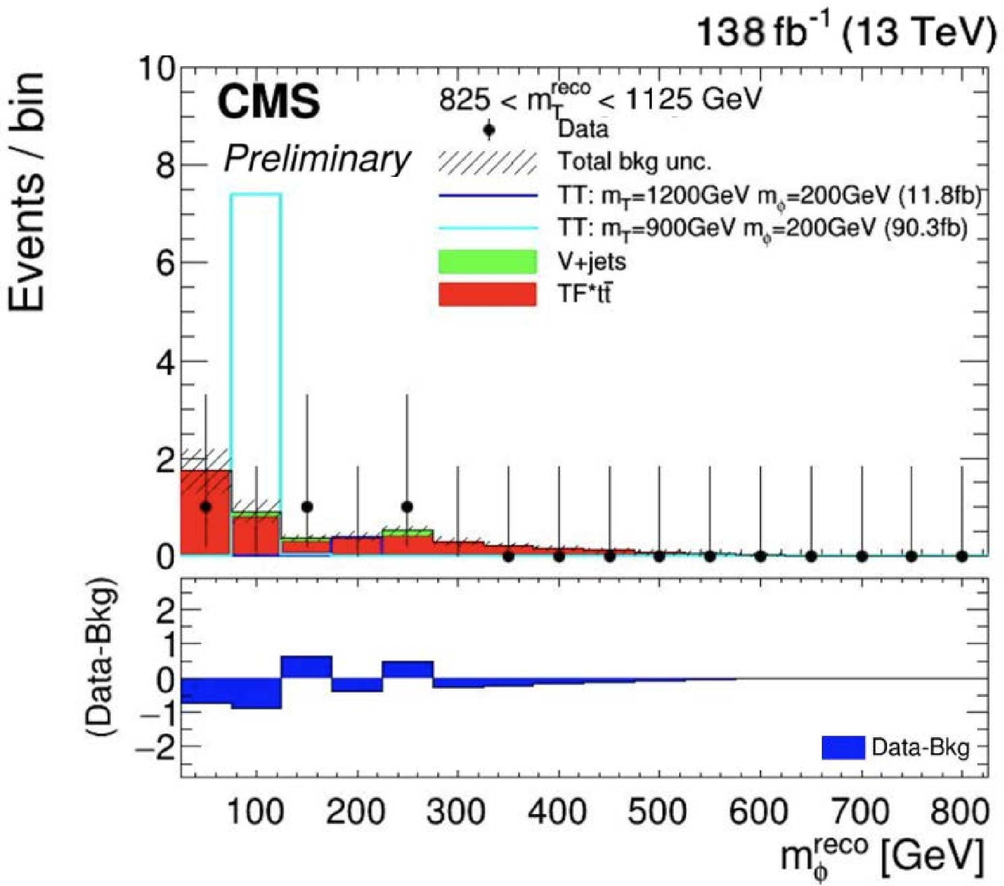
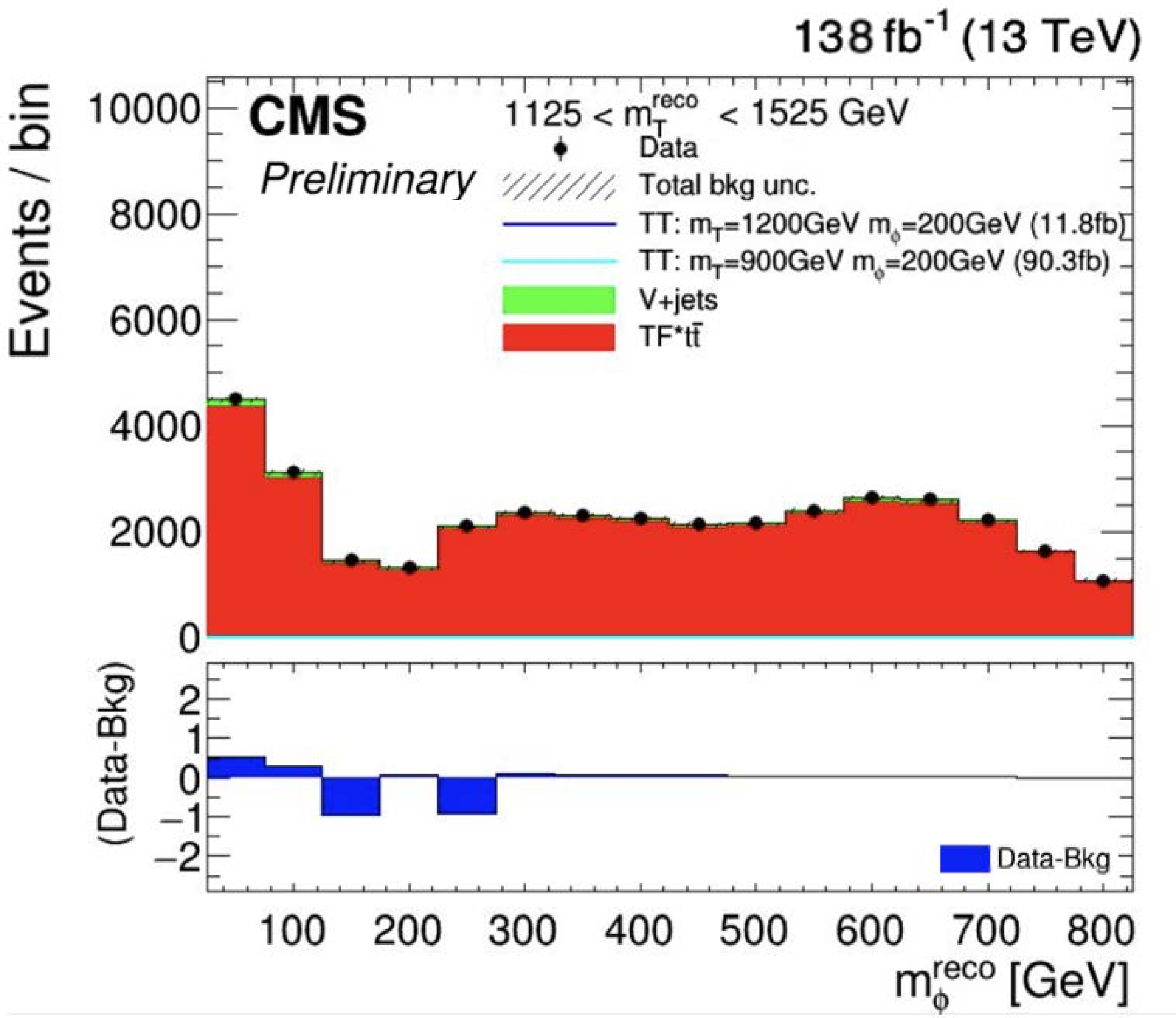
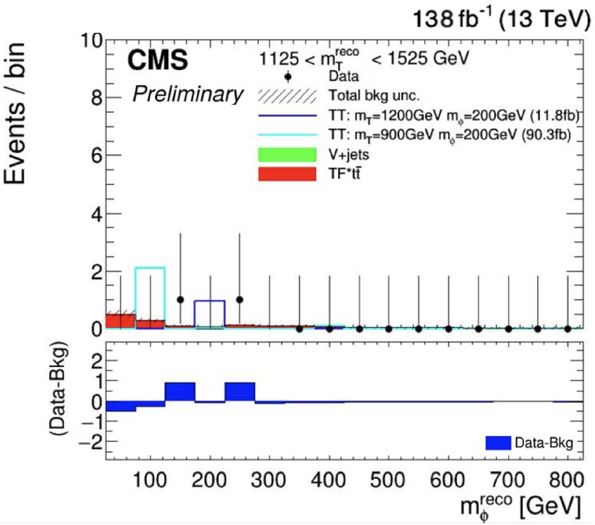
Figure 4:
Comparison of data and the postfit background prediction from the background-only fit in the VR. The VR-CR (left) and VR-SR (right) regions are shown. The distributions are projected onto $ m^\mathrm{reco}_{\phi} $ in three intervals of $ m^\mathrm{reco}_{{\mathrm{T}} } $: 625 $ < m^\mathrm{reco}_{{\mathrm{T}} } < $ 825 GeV (top), 825 $ < m^\mathrm{reco}_{{\mathrm{T}} } < $ 1125 GeV (middle), and 1125 $ < m^\mathrm{reco}_{{\mathrm{T}} } < $ 1525 GeV (bottom). The $ \mathrm{t}\overline{\mathrm{t}} $ component scaled by the transfer function is shown in red and the $ \mathrm{W}/\mathrm{Z} $+jets contribution in green. Signal distributions for the mass hypotheses $ m_{{\mathrm{T}} }= $ 1200 GeV, $ m_{\phi}= $ 200 GeV and $ m_{{\mathrm{T}} }= $ 900 GeV, $ m_{\phi}= $ 100 GeV are overlaid as thin lines. The lower panels show the difference between the data and the background prediction. |
png pdf |
Figure 4-a:
Comparison of data and the postfit background prediction from the background-only fit in the VR. The VR-CR (left) and VR-SR (right) regions are shown. The distributions are projected onto $ m^\mathrm{reco}_{\phi} $ in three intervals of $ m^\mathrm{reco}_{{\mathrm{T}} } $: 625 $ < m^\mathrm{reco}_{{\mathrm{T}} } < $ 825 GeV (top), 825 $ < m^\mathrm{reco}_{{\mathrm{T}} } < $ 1125 GeV (middle), and 1125 $ < m^\mathrm{reco}_{{\mathrm{T}} } < $ 1525 GeV (bottom). The $ \mathrm{t}\overline{\mathrm{t}} $ component scaled by the transfer function is shown in red and the $ \mathrm{W}/\mathrm{Z} $+jets contribution in green. Signal distributions for the mass hypotheses $ m_{{\mathrm{T}} }= $ 1200 GeV, $ m_{\phi}= $ 200 GeV and $ m_{{\mathrm{T}} }= $ 900 GeV, $ m_{\phi}= $ 100 GeV are overlaid as thin lines. The lower panels show the difference between the data and the background prediction. |
png pdf |
Figure 4-b:
Comparison of data and the postfit background prediction from the background-only fit in the VR. The VR-CR (left) and VR-SR (right) regions are shown. The distributions are projected onto $ m^\mathrm{reco}_{\phi} $ in three intervals of $ m^\mathrm{reco}_{{\mathrm{T}} } $: 625 $ < m^\mathrm{reco}_{{\mathrm{T}} } < $ 825 GeV (top), 825 $ < m^\mathrm{reco}_{{\mathrm{T}} } < $ 1125 GeV (middle), and 1125 $ < m^\mathrm{reco}_{{\mathrm{T}} } < $ 1525 GeV (bottom). The $ \mathrm{t}\overline{\mathrm{t}} $ component scaled by the transfer function is shown in red and the $ \mathrm{W}/\mathrm{Z} $+jets contribution in green. Signal distributions for the mass hypotheses $ m_{{\mathrm{T}} }= $ 1200 GeV, $ m_{\phi}= $ 200 GeV and $ m_{{\mathrm{T}} }= $ 900 GeV, $ m_{\phi}= $ 100 GeV are overlaid as thin lines. The lower panels show the difference between the data and the background prediction. |
png pdf |
Figure 4-c:
Comparison of data and the postfit background prediction from the background-only fit in the VR. The VR-CR (left) and VR-SR (right) regions are shown. The distributions are projected onto $ m^\mathrm{reco}_{\phi} $ in three intervals of $ m^\mathrm{reco}_{{\mathrm{T}} } $: 625 $ < m^\mathrm{reco}_{{\mathrm{T}} } < $ 825 GeV (top), 825 $ < m^\mathrm{reco}_{{\mathrm{T}} } < $ 1125 GeV (middle), and 1125 $ < m^\mathrm{reco}_{{\mathrm{T}} } < $ 1525 GeV (bottom). The $ \mathrm{t}\overline{\mathrm{t}} $ component scaled by the transfer function is shown in red and the $ \mathrm{W}/\mathrm{Z} $+jets contribution in green. Signal distributions for the mass hypotheses $ m_{{\mathrm{T}} }= $ 1200 GeV, $ m_{\phi}= $ 200 GeV and $ m_{{\mathrm{T}} }= $ 900 GeV, $ m_{\phi}= $ 100 GeV are overlaid as thin lines. The lower panels show the difference between the data and the background prediction. |
png pdf |
Figure 4-d:
Comparison of data and the postfit background prediction from the background-only fit in the VR. The VR-CR (left) and VR-SR (right) regions are shown. The distributions are projected onto $ m^\mathrm{reco}_{\phi} $ in three intervals of $ m^\mathrm{reco}_{{\mathrm{T}} } $: 625 $ < m^\mathrm{reco}_{{\mathrm{T}} } < $ 825 GeV (top), 825 $ < m^\mathrm{reco}_{{\mathrm{T}} } < $ 1125 GeV (middle), and 1125 $ < m^\mathrm{reco}_{{\mathrm{T}} } < $ 1525 GeV (bottom). The $ \mathrm{t}\overline{\mathrm{t}} $ component scaled by the transfer function is shown in red and the $ \mathrm{W}/\mathrm{Z} $+jets contribution in green. Signal distributions for the mass hypotheses $ m_{{\mathrm{T}} }= $ 1200 GeV, $ m_{\phi}= $ 200 GeV and $ m_{{\mathrm{T}} }= $ 900 GeV, $ m_{\phi}= $ 100 GeV are overlaid as thin lines. The lower panels show the difference between the data and the background prediction. |
png pdf |
Figure 4-e:
Comparison of data and the postfit background prediction from the background-only fit in the VR. The VR-CR (left) and VR-SR (right) regions are shown. The distributions are projected onto $ m^\mathrm{reco}_{\phi} $ in three intervals of $ m^\mathrm{reco}_{{\mathrm{T}} } $: 625 $ < m^\mathrm{reco}_{{\mathrm{T}} } < $ 825 GeV (top), 825 $ < m^\mathrm{reco}_{{\mathrm{T}} } < $ 1125 GeV (middle), and 1125 $ < m^\mathrm{reco}_{{\mathrm{T}} } < $ 1525 GeV (bottom). The $ \mathrm{t}\overline{\mathrm{t}} $ component scaled by the transfer function is shown in red and the $ \mathrm{W}/\mathrm{Z} $+jets contribution in green. Signal distributions for the mass hypotheses $ m_{{\mathrm{T}} }= $ 1200 GeV, $ m_{\phi}= $ 200 GeV and $ m_{{\mathrm{T}} }= $ 900 GeV, $ m_{\phi}= $ 100 GeV are overlaid as thin lines. The lower panels show the difference between the data and the background prediction. |
png pdf |
Figure 4-f:
Comparison of data and the postfit background prediction from the background-only fit in the VR. The VR-CR (left) and VR-SR (right) regions are shown. The distributions are projected onto $ m^\mathrm{reco}_{\phi} $ in three intervals of $ m^\mathrm{reco}_{{\mathrm{T}} } $: 625 $ < m^\mathrm{reco}_{{\mathrm{T}} } < $ 825 GeV (top), 825 $ < m^\mathrm{reco}_{{\mathrm{T}} } < $ 1125 GeV (middle), and 1125 $ < m^\mathrm{reco}_{{\mathrm{T}} } < $ 1525 GeV (bottom). The $ \mathrm{t}\overline{\mathrm{t}} $ component scaled by the transfer function is shown in red and the $ \mathrm{W}/\mathrm{Z} $+jets contribution in green. Signal distributions for the mass hypotheses $ m_{{\mathrm{T}} }= $ 1200 GeV, $ m_{\phi}= $ 200 GeV and $ m_{{\mathrm{T}} }= $ 900 GeV, $ m_{\phi}= $ 100 GeV are overlaid as thin lines. The lower panels show the difference between the data and the background prediction. |
png pdf |
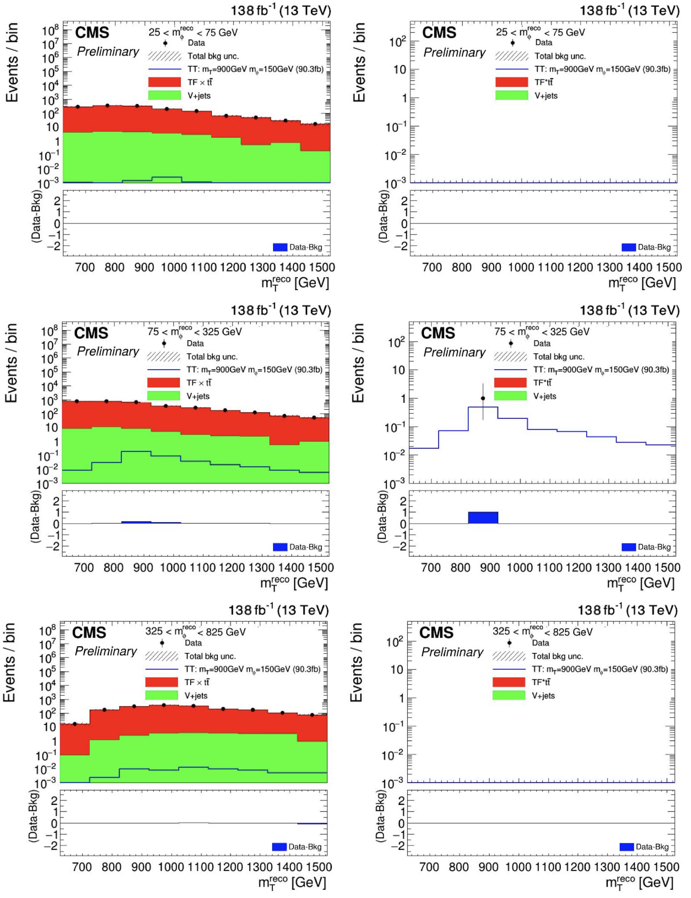
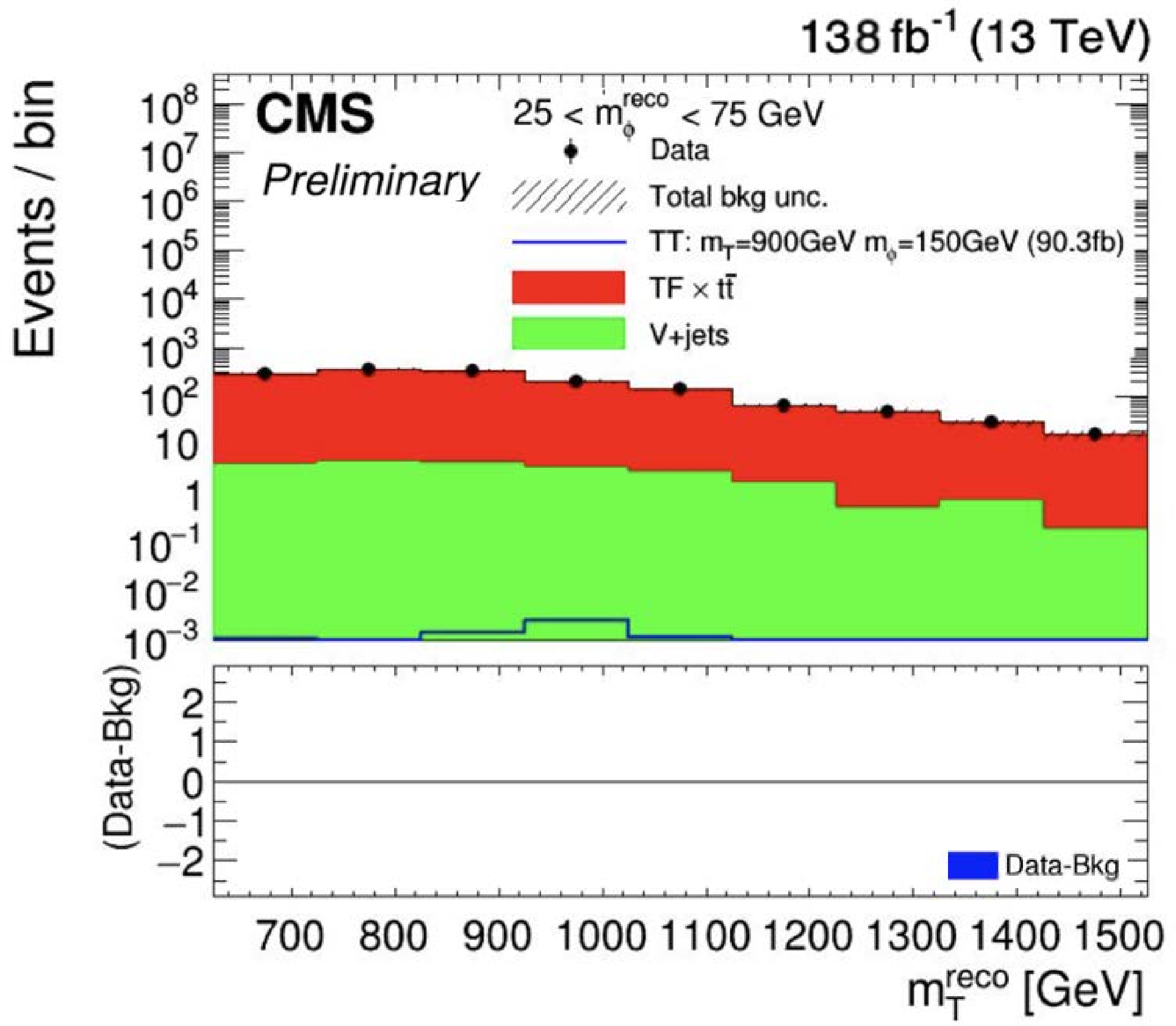
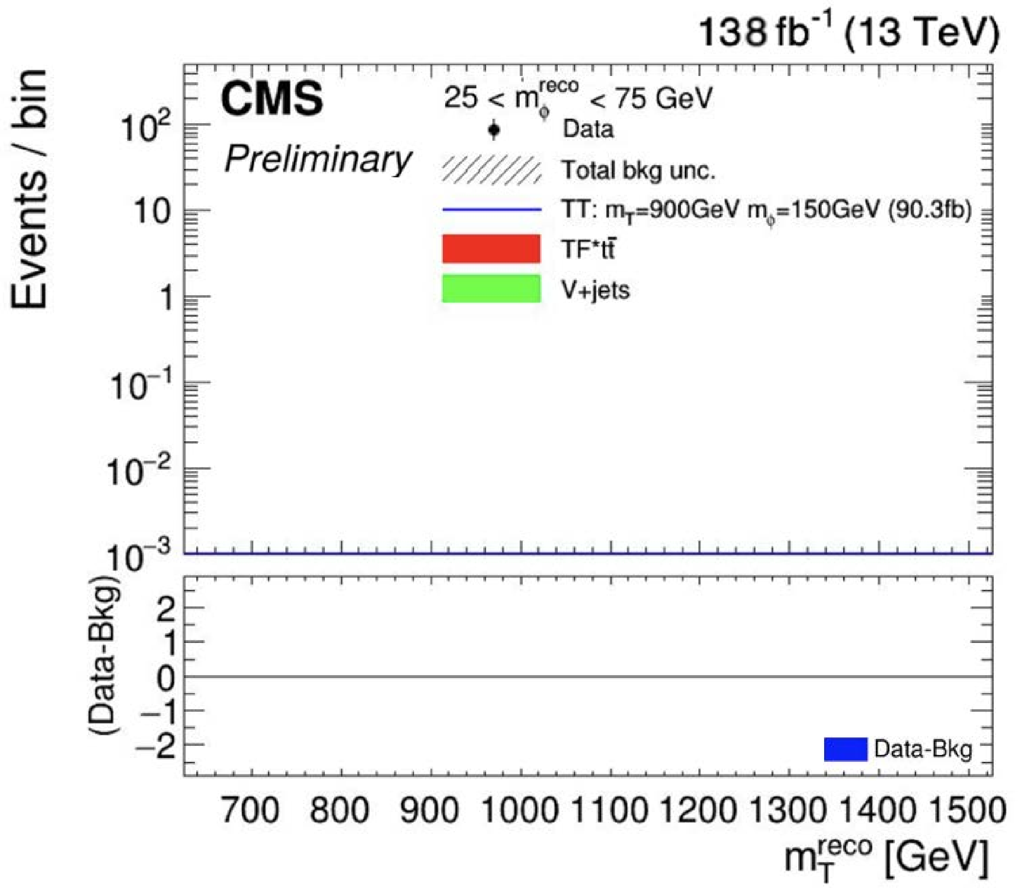
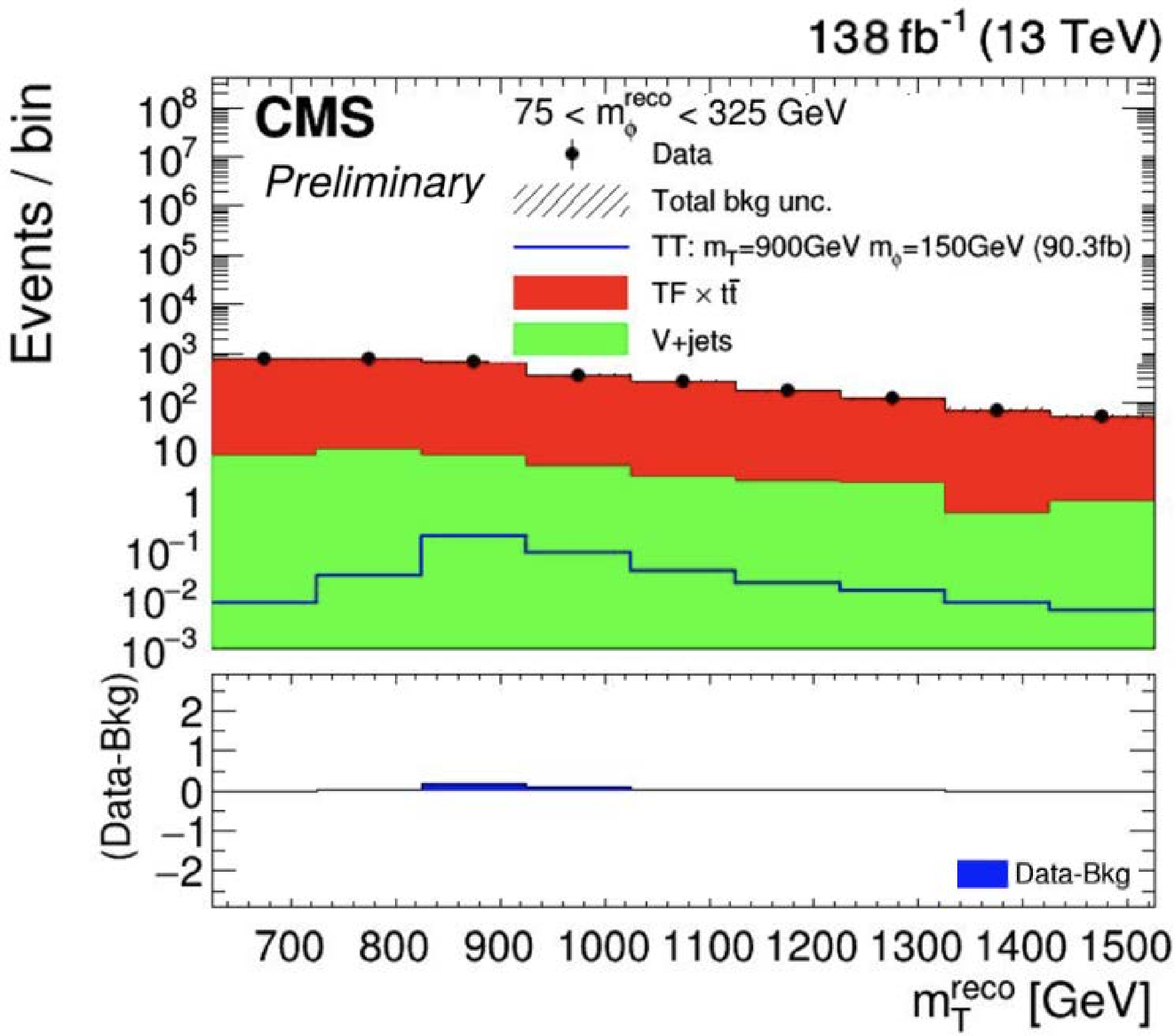
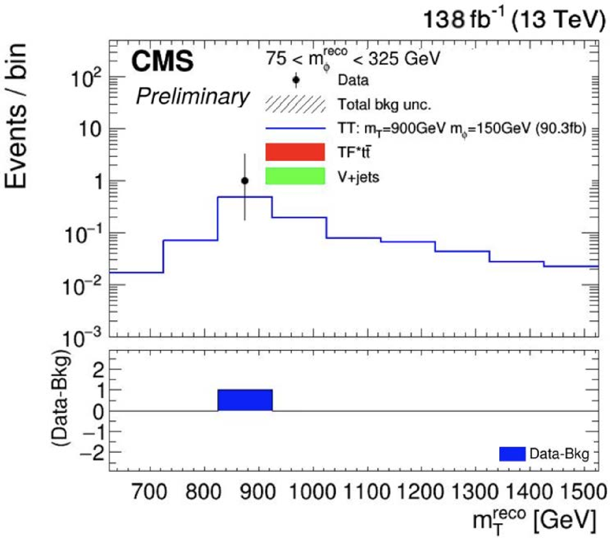
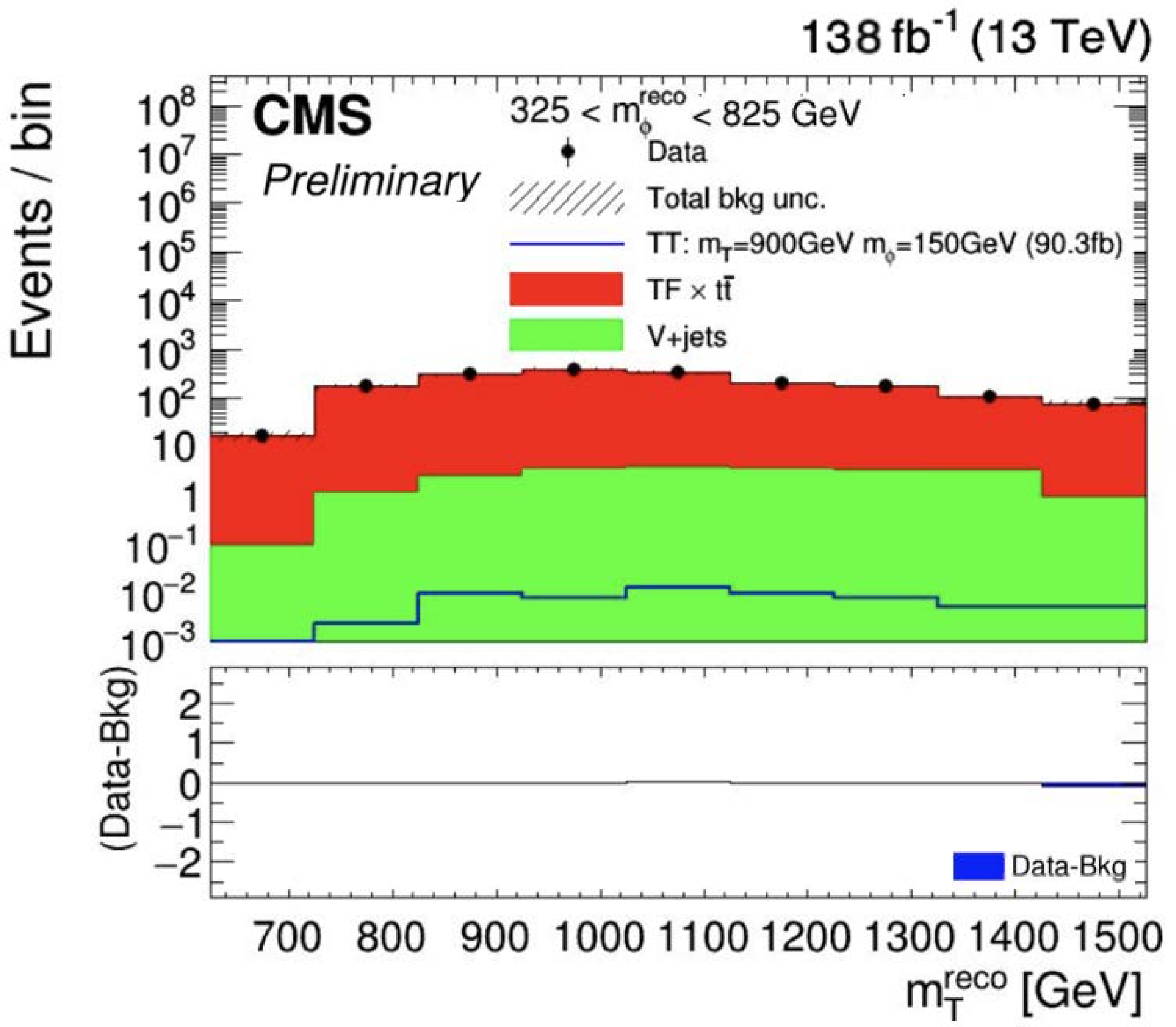
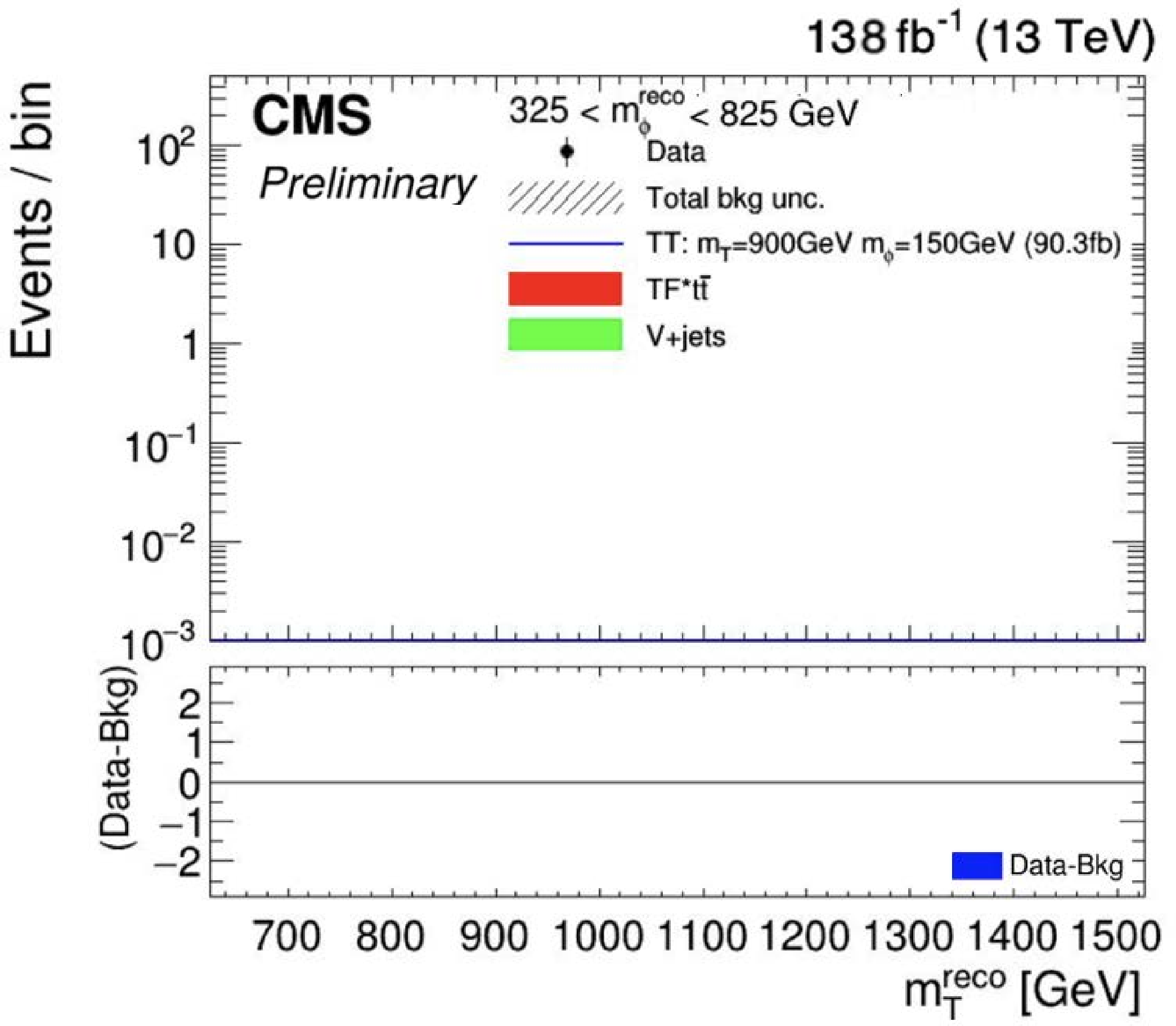
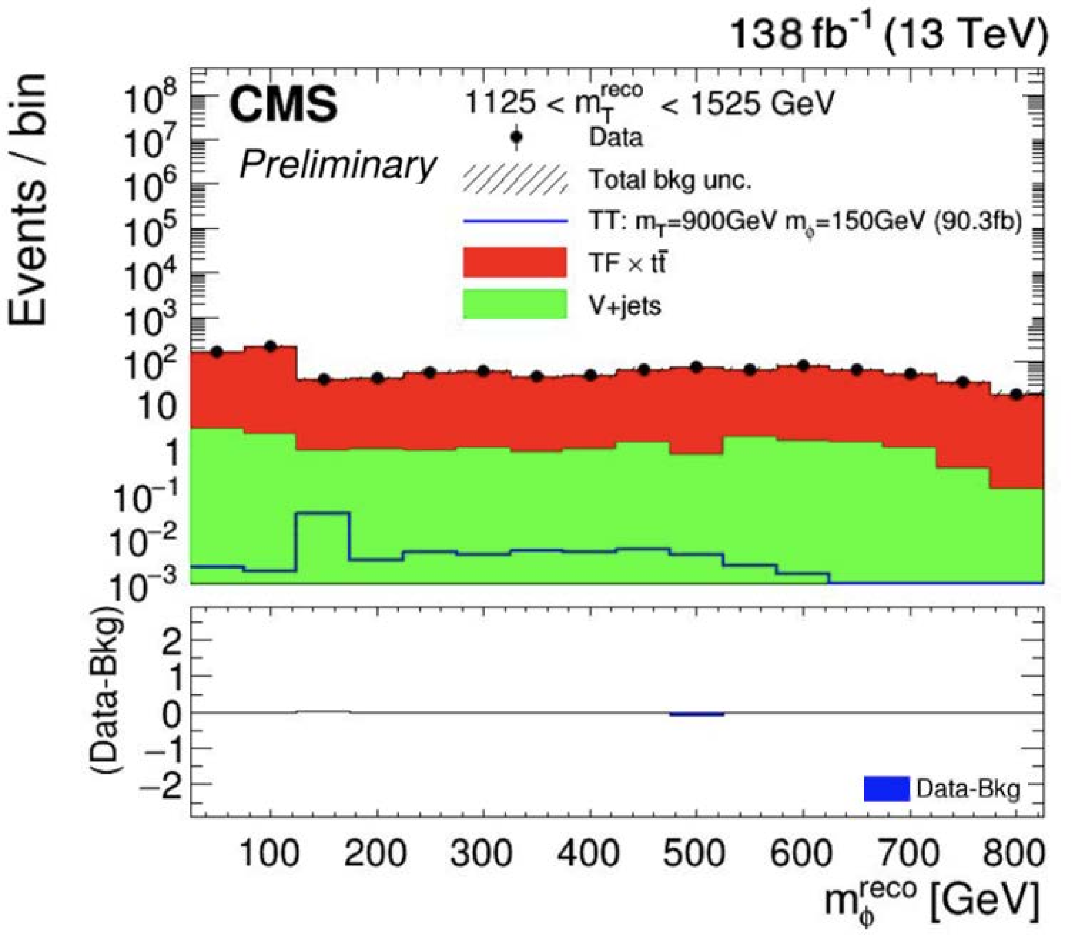
Figure 5:
Comparison of the data and the postfit background prediction projected onto $ m^\mathrm{reco}_{{\mathrm{T}} } $ for the signal hypothesis $ m_{{\mathrm{T}} }= $ 900 GeV and $ m_{\phi}= $ 150 GeV. The CR (left) and SR (right) regions are shown. The distributions are shown in three intervals of $ m^\mathrm{reco}_{\phi} $: 25 $ < m^\mathrm{reco}_{\phi} < $ 75 GeV (top), 75 $ < m^\mathrm{reco}_{\phi} < $ 325 GeV (middle), and 325 $ < m^\mathrm{reco}_{\phi} < $ 625 GeV (bottom). The transferred $ \mathrm{t}\overline{\mathrm{t}} $ contribution is shown in red and the $ \mathrm{W}/\mathrm{Z} $+jets contribution in green. Signal distributions are overlaid as thin lines. The lower panels show the difference between the data and the background prediction. |
png pdf |
Figure 5-a:
Comparison of the data and the postfit background prediction projected onto $ m^\mathrm{reco}_{{\mathrm{T}} } $ for the signal hypothesis $ m_{{\mathrm{T}} }= $ 900 GeV and $ m_{\phi}= $ 150 GeV. The CR (left) and SR (right) regions are shown. The distributions are shown in three intervals of $ m^\mathrm{reco}_{\phi} $: 25 $ < m^\mathrm{reco}_{\phi} < $ 75 GeV (top), 75 $ < m^\mathrm{reco}_{\phi} < $ 325 GeV (middle), and 325 $ < m^\mathrm{reco}_{\phi} < $ 625 GeV (bottom). The transferred $ \mathrm{t}\overline{\mathrm{t}} $ contribution is shown in red and the $ \mathrm{W}/\mathrm{Z} $+jets contribution in green. Signal distributions are overlaid as thin lines. The lower panels show the difference between the data and the background prediction. |
png pdf |
Figure 5-b:
Comparison of the data and the postfit background prediction projected onto $ m^\mathrm{reco}_{{\mathrm{T}} } $ for the signal hypothesis $ m_{{\mathrm{T}} }= $ 900 GeV and $ m_{\phi}= $ 150 GeV. The CR (left) and SR (right) regions are shown. The distributions are shown in three intervals of $ m^\mathrm{reco}_{\phi} $: 25 $ < m^\mathrm{reco}_{\phi} < $ 75 GeV (top), 75 $ < m^\mathrm{reco}_{\phi} < $ 325 GeV (middle), and 325 $ < m^\mathrm{reco}_{\phi} < $ 625 GeV (bottom). The transferred $ \mathrm{t}\overline{\mathrm{t}} $ contribution is shown in red and the $ \mathrm{W}/\mathrm{Z} $+jets contribution in green. Signal distributions are overlaid as thin lines. The lower panels show the difference between the data and the background prediction. |
png pdf |
Figure 5-c:
Comparison of the data and the postfit background prediction projected onto $ m^\mathrm{reco}_{{\mathrm{T}} } $ for the signal hypothesis $ m_{{\mathrm{T}} }= $ 900 GeV and $ m_{\phi}= $ 150 GeV. The CR (left) and SR (right) regions are shown. The distributions are shown in three intervals of $ m^\mathrm{reco}_{\phi} $: 25 $ < m^\mathrm{reco}_{\phi} < $ 75 GeV (top), 75 $ < m^\mathrm{reco}_{\phi} < $ 325 GeV (middle), and 325 $ < m^\mathrm{reco}_{\phi} < $ 625 GeV (bottom). The transferred $ \mathrm{t}\overline{\mathrm{t}} $ contribution is shown in red and the $ \mathrm{W}/\mathrm{Z} $+jets contribution in green. Signal distributions are overlaid as thin lines. The lower panels show the difference between the data and the background prediction. |
png pdf |
Figure 5-d:
Comparison of the data and the postfit background prediction projected onto $ m^\mathrm{reco}_{{\mathrm{T}} } $ for the signal hypothesis $ m_{{\mathrm{T}} }= $ 900 GeV and $ m_{\phi}= $ 150 GeV. The CR (left) and SR (right) regions are shown. The distributions are shown in three intervals of $ m^\mathrm{reco}_{\phi} $: 25 $ < m^\mathrm{reco}_{\phi} < $ 75 GeV (top), 75 $ < m^\mathrm{reco}_{\phi} < $ 325 GeV (middle), and 325 $ < m^\mathrm{reco}_{\phi} < $ 625 GeV (bottom). The transferred $ \mathrm{t}\overline{\mathrm{t}} $ contribution is shown in red and the $ \mathrm{W}/\mathrm{Z} $+jets contribution in green. Signal distributions are overlaid as thin lines. The lower panels show the difference between the data and the background prediction. |
png pdf |
Figure 5-e:
Comparison of the data and the postfit background prediction projected onto $ m^\mathrm{reco}_{{\mathrm{T}} } $ for the signal hypothesis $ m_{{\mathrm{T}} }= $ 900 GeV and $ m_{\phi}= $ 150 GeV. The CR (left) and SR (right) regions are shown. The distributions are shown in three intervals of $ m^\mathrm{reco}_{\phi} $: 25 $ < m^\mathrm{reco}_{\phi} < $ 75 GeV (top), 75 $ < m^\mathrm{reco}_{\phi} < $ 325 GeV (middle), and 325 $ < m^\mathrm{reco}_{\phi} < $ 625 GeV (bottom). The transferred $ \mathrm{t}\overline{\mathrm{t}} $ contribution is shown in red and the $ \mathrm{W}/\mathrm{Z} $+jets contribution in green. Signal distributions are overlaid as thin lines. The lower panels show the difference between the data and the background prediction. |
png pdf |
Figure 5-f:
Comparison of the data and the postfit background prediction projected onto $ m^\mathrm{reco}_{{\mathrm{T}} } $ for the signal hypothesis $ m_{{\mathrm{T}} }= $ 900 GeV and $ m_{\phi}= $ 150 GeV. The CR (left) and SR (right) regions are shown. The distributions are shown in three intervals of $ m^\mathrm{reco}_{\phi} $: 25 $ < m^\mathrm{reco}_{\phi} < $ 75 GeV (top), 75 $ < m^\mathrm{reco}_{\phi} < $ 325 GeV (middle), and 325 $ < m^\mathrm{reco}_{\phi} < $ 625 GeV (bottom). The transferred $ \mathrm{t}\overline{\mathrm{t}} $ contribution is shown in red and the $ \mathrm{W}/\mathrm{Z} $+jets contribution in green. Signal distributions are overlaid as thin lines. The lower panels show the difference between the data and the background prediction. |
png pdf |
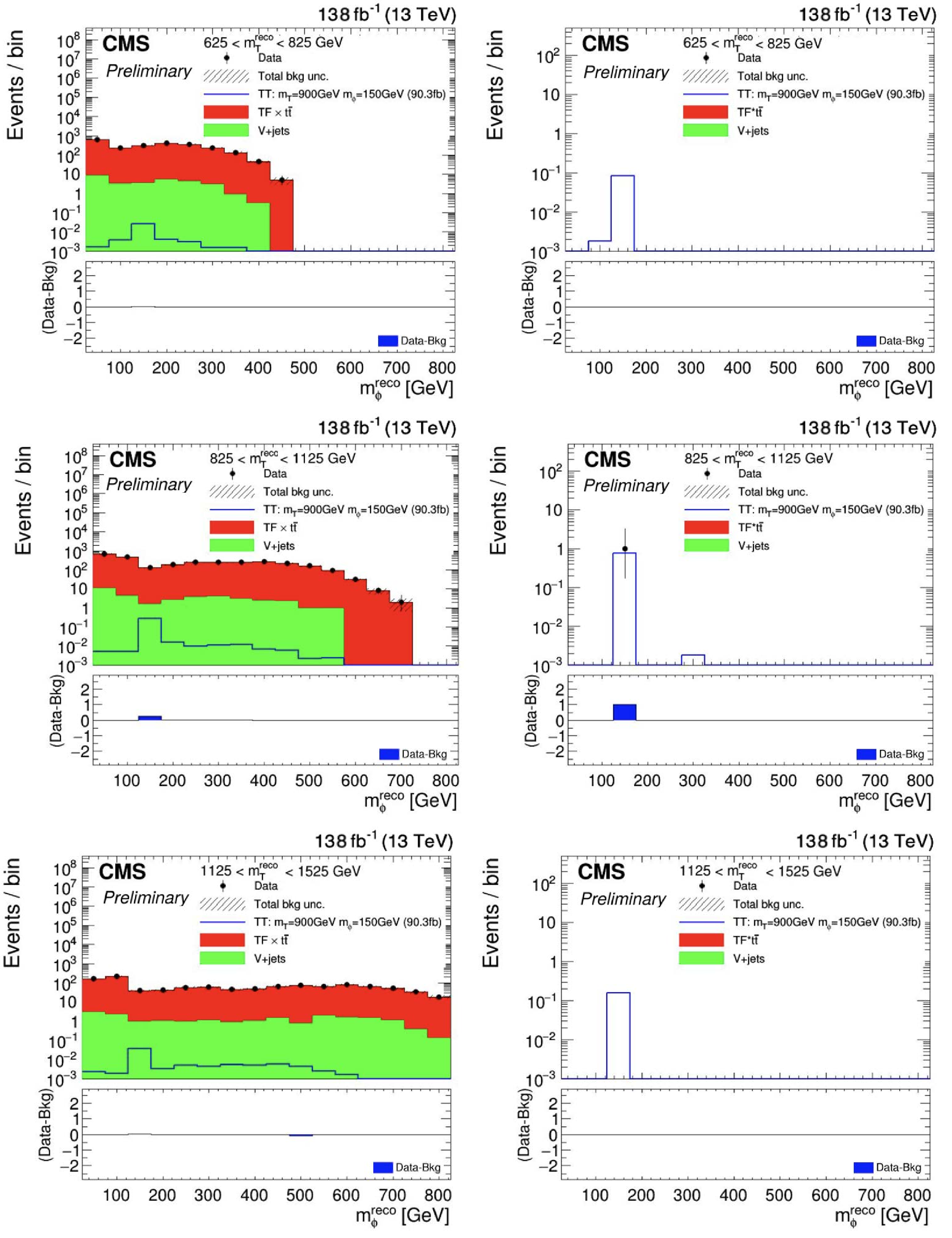
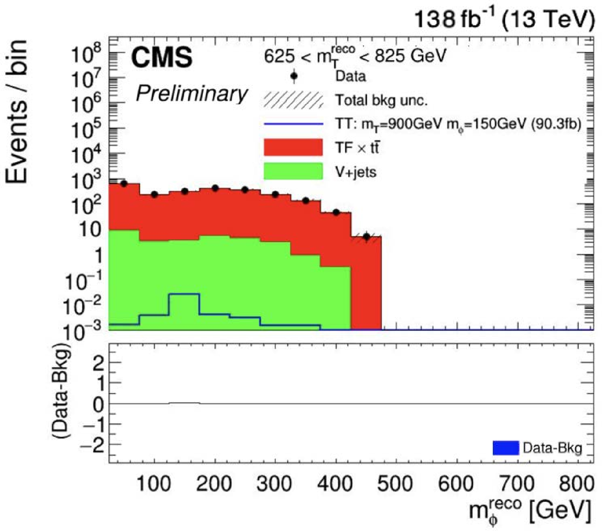
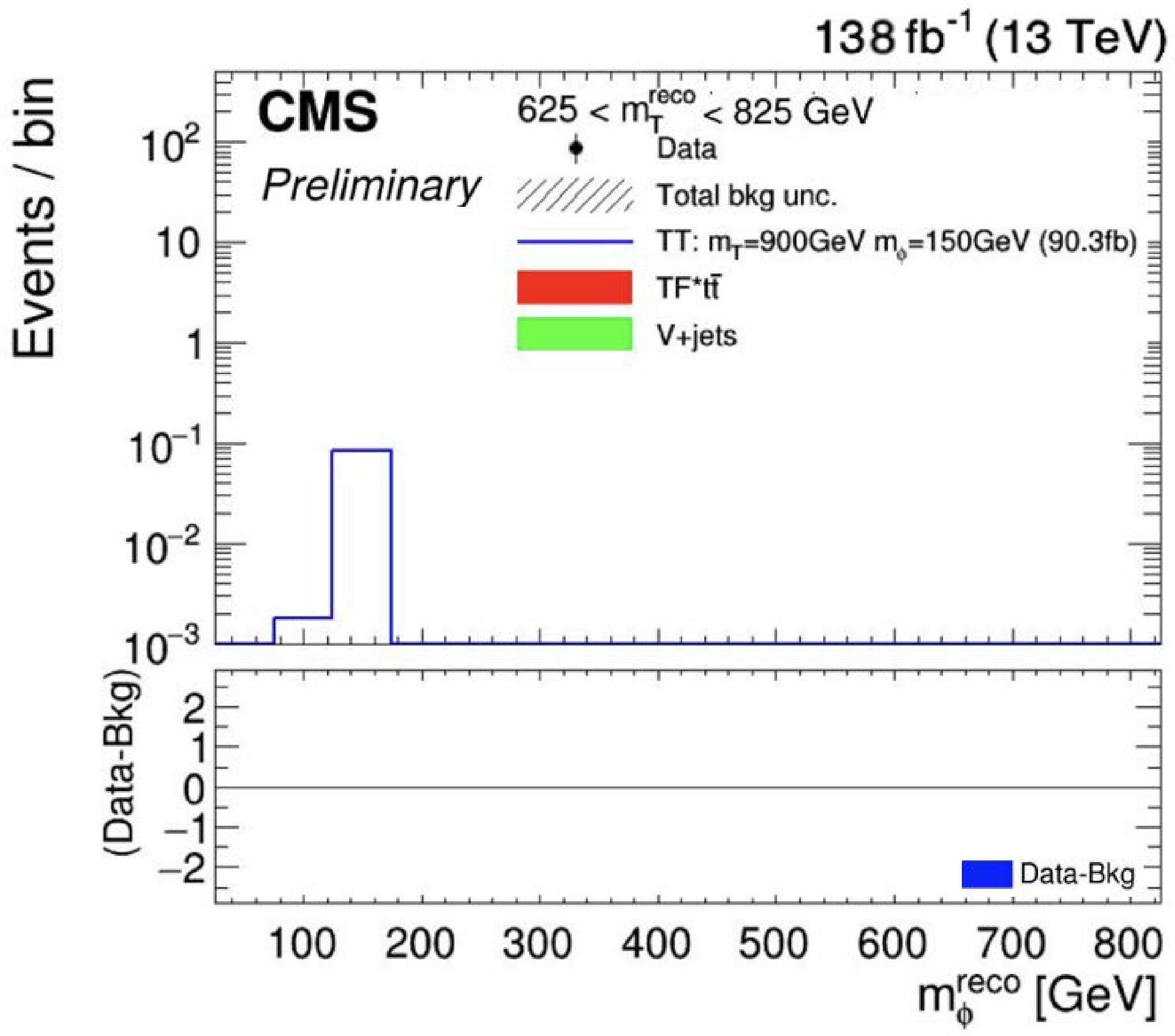
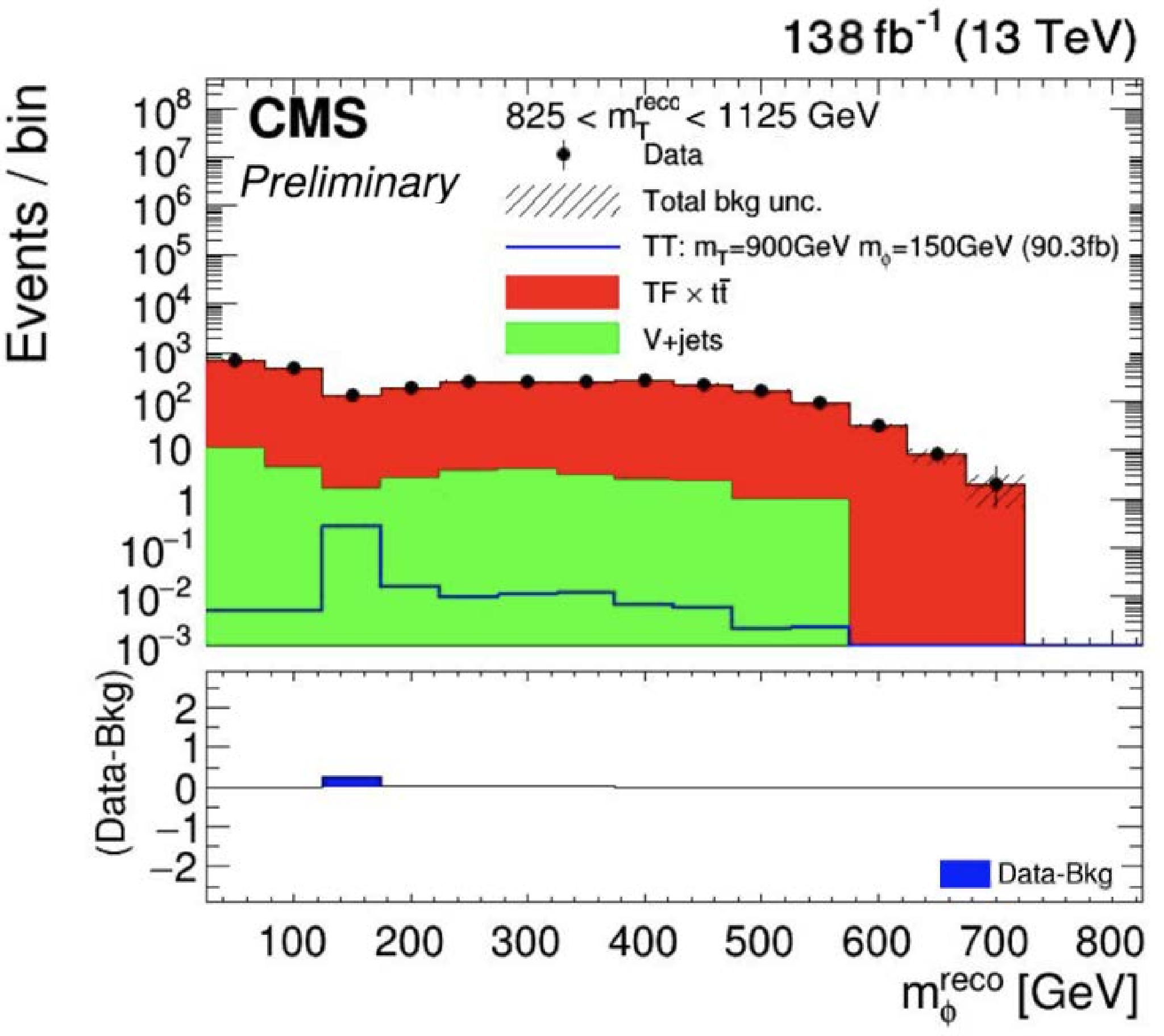
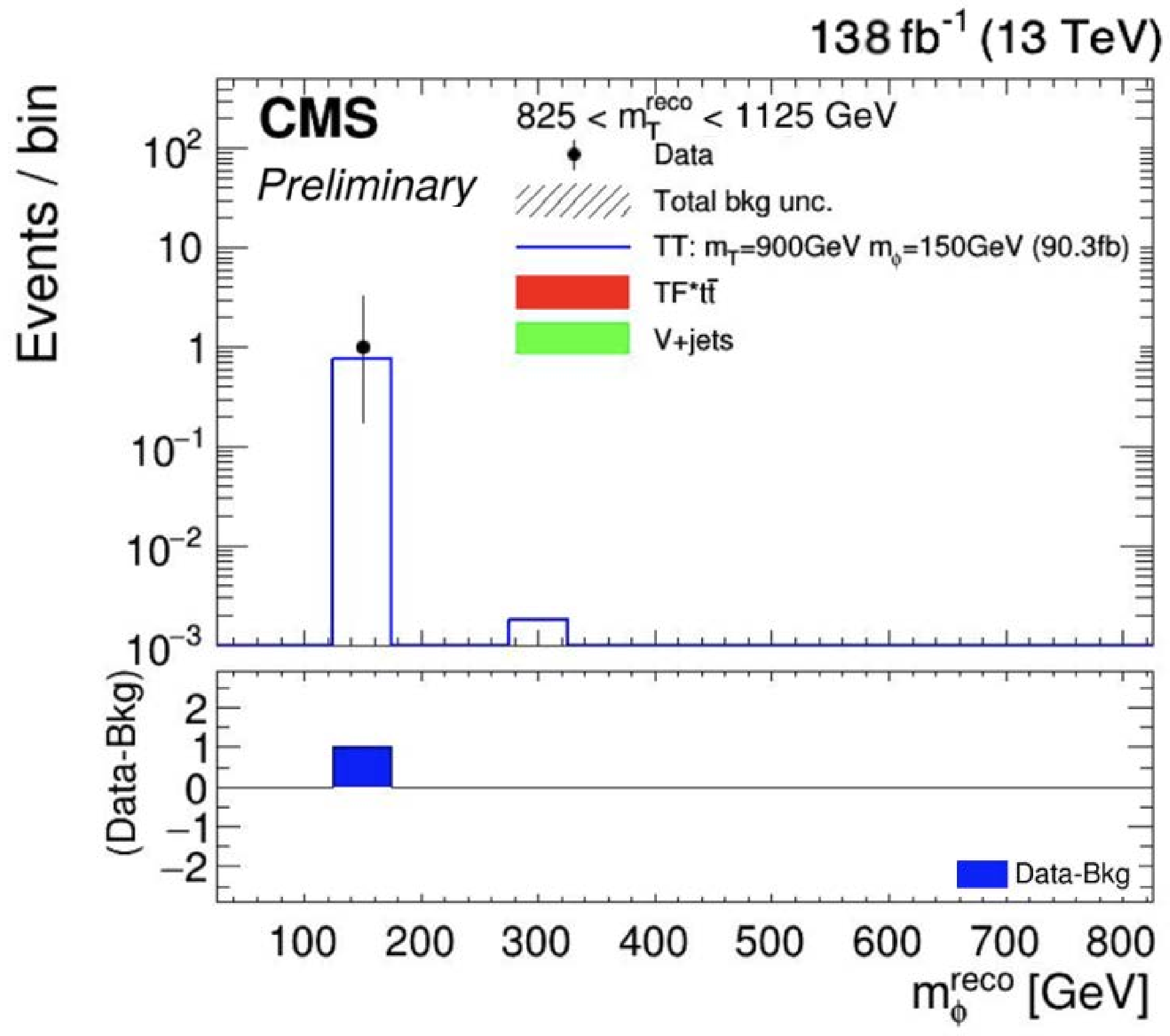
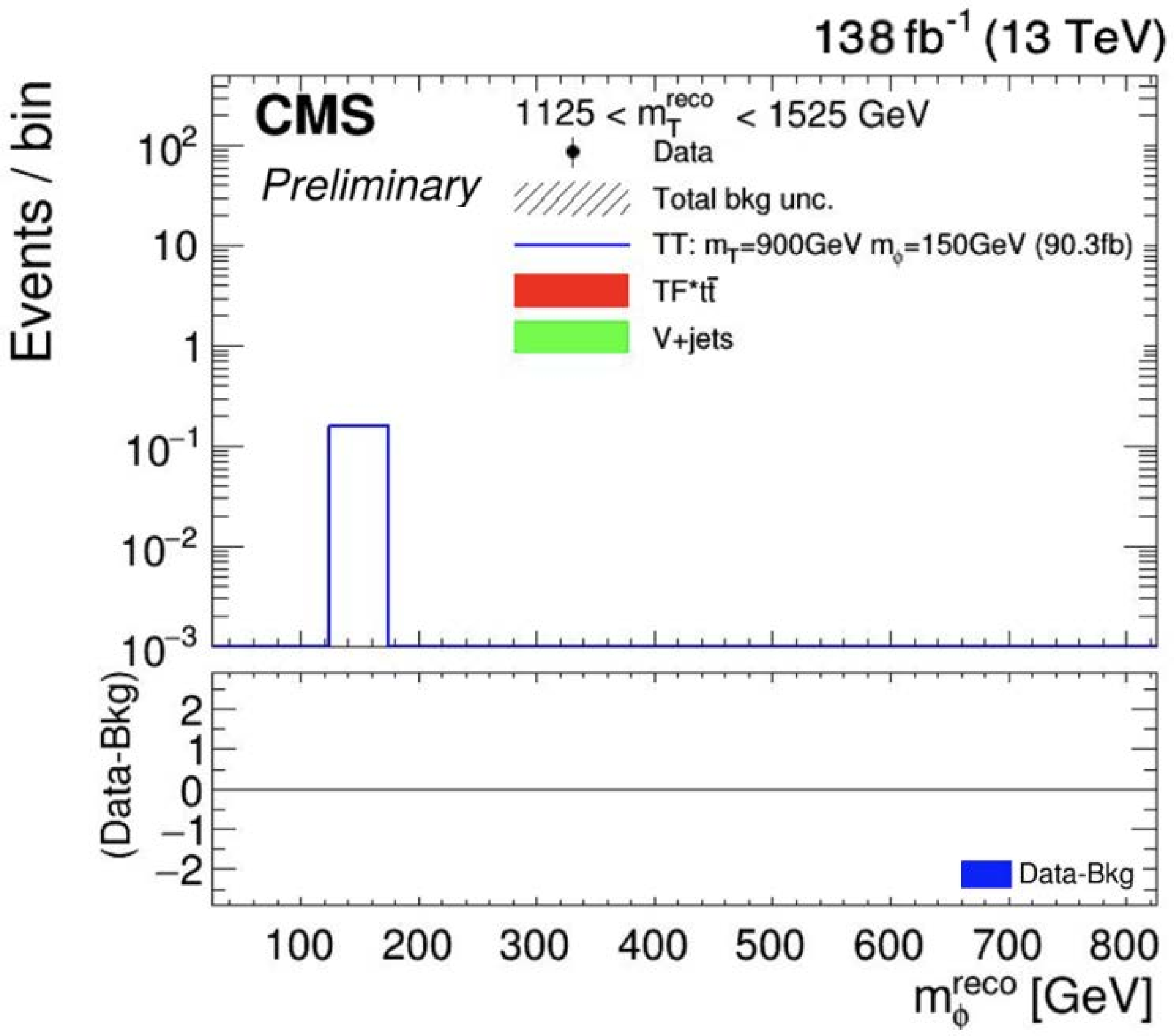
Figure 6:
Comparison of the data and the postfit background prediction projected onto $ m^\mathrm{reco}_{\phi} $ for the signal hypothesis $ m_{{\mathrm{T}} }= $ 900 GeV and $ m_{\phi}= $ 150 GeV. The CR (left) and SR (right) regions are shown. The distributions are shown in three intervals of $ m^\mathrm{reco}_{{\mathrm{T}} } $: 625 $ < m^\mathrm{reco}_{{\mathrm{T}} } < $ 825 GeV (top), 825 $ < m^\mathrm{reco}_{{\mathrm{T}} } < $ 1125 GeV (middle), and 1125 $ < m^\mathrm{reco}_{{\mathrm{T}} } < $ 1525 GeV (bottom). The transferred $ \mathrm{t}\overline{\mathrm{t}} $ contribution is shown in red and the $ \mathrm{W}/\mathrm{Z} $+jets contribution in green. Signal distributions are overlaid as thin lines. The lower panels show the difference between the data and the background prediction. |
png pdf |
Figure 6-a:
Comparison of the data and the postfit background prediction projected onto $ m^\mathrm{reco}_{\phi} $ for the signal hypothesis $ m_{{\mathrm{T}} }= $ 900 GeV and $ m_{\phi}= $ 150 GeV. The CR (left) and SR (right) regions are shown. The distributions are shown in three intervals of $ m^\mathrm{reco}_{{\mathrm{T}} } $: 625 $ < m^\mathrm{reco}_{{\mathrm{T}} } < $ 825 GeV (top), 825 $ < m^\mathrm{reco}_{{\mathrm{T}} } < $ 1125 GeV (middle), and 1125 $ < m^\mathrm{reco}_{{\mathrm{T}} } < $ 1525 GeV (bottom). The transferred $ \mathrm{t}\overline{\mathrm{t}} $ contribution is shown in red and the $ \mathrm{W}/\mathrm{Z} $+jets contribution in green. Signal distributions are overlaid as thin lines. The lower panels show the difference between the data and the background prediction. |
png pdf |
Figure 6-b:
Comparison of the data and the postfit background prediction projected onto $ m^\mathrm{reco}_{\phi} $ for the signal hypothesis $ m_{{\mathrm{T}} }= $ 900 GeV and $ m_{\phi}= $ 150 GeV. The CR (left) and SR (right) regions are shown. The distributions are shown in three intervals of $ m^\mathrm{reco}_{{\mathrm{T}} } $: 625 $ < m^\mathrm{reco}_{{\mathrm{T}} } < $ 825 GeV (top), 825 $ < m^\mathrm{reco}_{{\mathrm{T}} } < $ 1125 GeV (middle), and 1125 $ < m^\mathrm{reco}_{{\mathrm{T}} } < $ 1525 GeV (bottom). The transferred $ \mathrm{t}\overline{\mathrm{t}} $ contribution is shown in red and the $ \mathrm{W}/\mathrm{Z} $+jets contribution in green. Signal distributions are overlaid as thin lines. The lower panels show the difference between the data and the background prediction. |
png pdf |
Figure 6-c:
Comparison of the data and the postfit background prediction projected onto $ m^\mathrm{reco}_{\phi} $ for the signal hypothesis $ m_{{\mathrm{T}} }= $ 900 GeV and $ m_{\phi}= $ 150 GeV. The CR (left) and SR (right) regions are shown. The distributions are shown in three intervals of $ m^\mathrm{reco}_{{\mathrm{T}} } $: 625 $ < m^\mathrm{reco}_{{\mathrm{T}} } < $ 825 GeV (top), 825 $ < m^\mathrm{reco}_{{\mathrm{T}} } < $ 1125 GeV (middle), and 1125 $ < m^\mathrm{reco}_{{\mathrm{T}} } < $ 1525 GeV (bottom). The transferred $ \mathrm{t}\overline{\mathrm{t}} $ contribution is shown in red and the $ \mathrm{W}/\mathrm{Z} $+jets contribution in green. Signal distributions are overlaid as thin lines. The lower panels show the difference between the data and the background prediction. |
png pdf |
Figure 6-d:
Comparison of the data and the postfit background prediction projected onto $ m^\mathrm{reco}_{\phi} $ for the signal hypothesis $ m_{{\mathrm{T}} }= $ 900 GeV and $ m_{\phi}= $ 150 GeV. The CR (left) and SR (right) regions are shown. The distributions are shown in three intervals of $ m^\mathrm{reco}_{{\mathrm{T}} } $: 625 $ < m^\mathrm{reco}_{{\mathrm{T}} } < $ 825 GeV (top), 825 $ < m^\mathrm{reco}_{{\mathrm{T}} } < $ 1125 GeV (middle), and 1125 $ < m^\mathrm{reco}_{{\mathrm{T}} } < $ 1525 GeV (bottom). The transferred $ \mathrm{t}\overline{\mathrm{t}} $ contribution is shown in red and the $ \mathrm{W}/\mathrm{Z} $+jets contribution in green. Signal distributions are overlaid as thin lines. The lower panels show the difference between the data and the background prediction. |
png pdf |
Figure 6-e:
Comparison of the data and the postfit background prediction projected onto $ m^\mathrm{reco}_{\phi} $ for the signal hypothesis $ m_{{\mathrm{T}} }= $ 900 GeV and $ m_{\phi}= $ 150 GeV. The CR (left) and SR (right) regions are shown. The distributions are shown in three intervals of $ m^\mathrm{reco}_{{\mathrm{T}} } $: 625 $ < m^\mathrm{reco}_{{\mathrm{T}} } < $ 825 GeV (top), 825 $ < m^\mathrm{reco}_{{\mathrm{T}} } < $ 1125 GeV (middle), and 1125 $ < m^\mathrm{reco}_{{\mathrm{T}} } < $ 1525 GeV (bottom). The transferred $ \mathrm{t}\overline{\mathrm{t}} $ contribution is shown in red and the $ \mathrm{W}/\mathrm{Z} $+jets contribution in green. Signal distributions are overlaid as thin lines. The lower panels show the difference between the data and the background prediction. |
png pdf |
Figure 6-f:
Comparison of the data and the postfit background prediction projected onto $ m^\mathrm{reco}_{\phi} $ for the signal hypothesis $ m_{{\mathrm{T}} }= $ 900 GeV and $ m_{\phi}= $ 150 GeV. The CR (left) and SR (right) regions are shown. The distributions are shown in three intervals of $ m^\mathrm{reco}_{{\mathrm{T}} } $: 625 $ < m^\mathrm{reco}_{{\mathrm{T}} } < $ 825 GeV (top), 825 $ < m^\mathrm{reco}_{{\mathrm{T}} } < $ 1125 GeV (middle), and 1125 $ < m^\mathrm{reco}_{{\mathrm{T}} } < $ 1525 GeV (bottom). The transferred $ \mathrm{t}\overline{\mathrm{t}} $ contribution is shown in red and the $ \mathrm{W}/\mathrm{Z} $+jets contribution in green. Signal distributions are overlaid as thin lines. The lower panels show the difference between the data and the background prediction. |
png pdf |
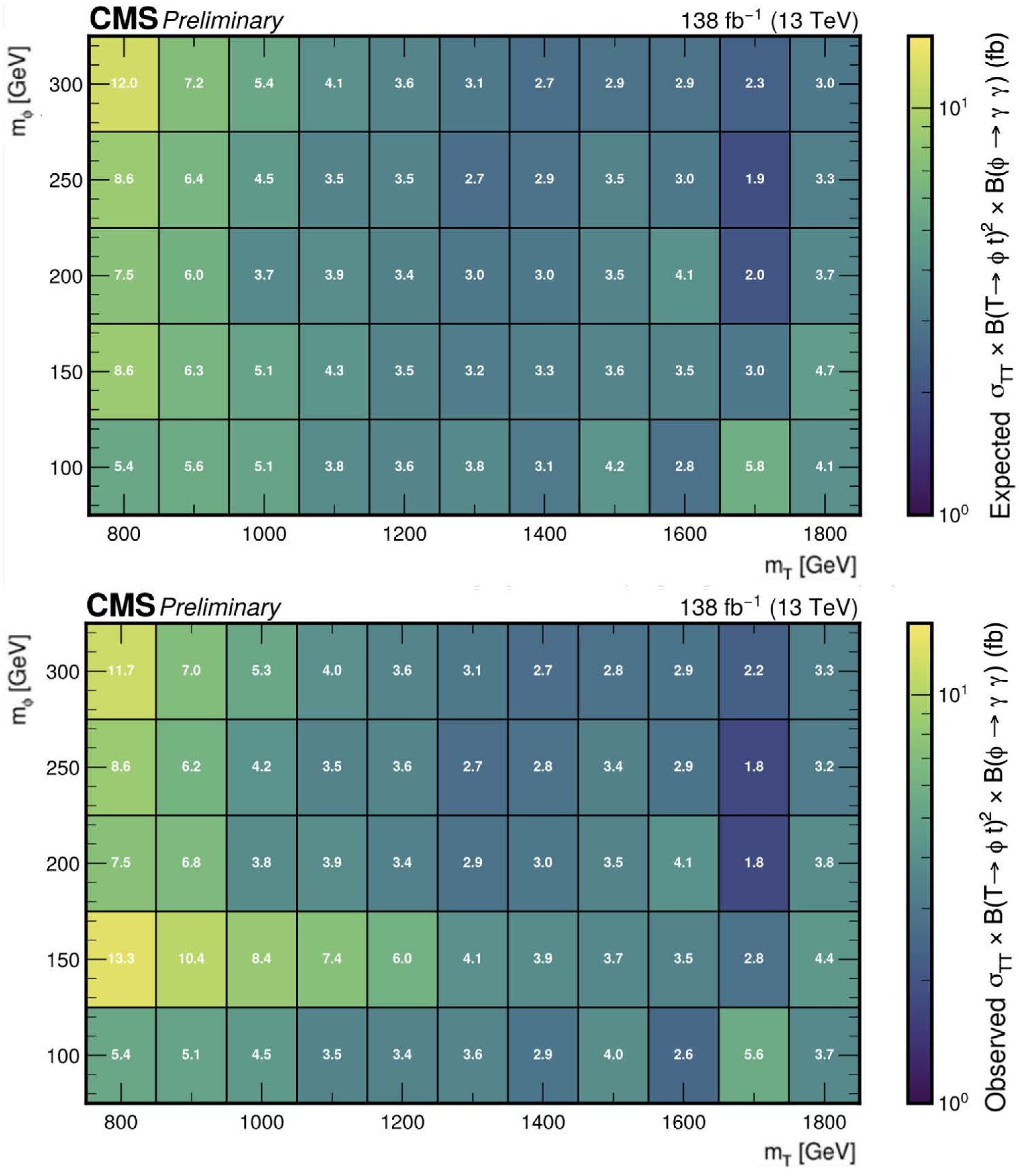
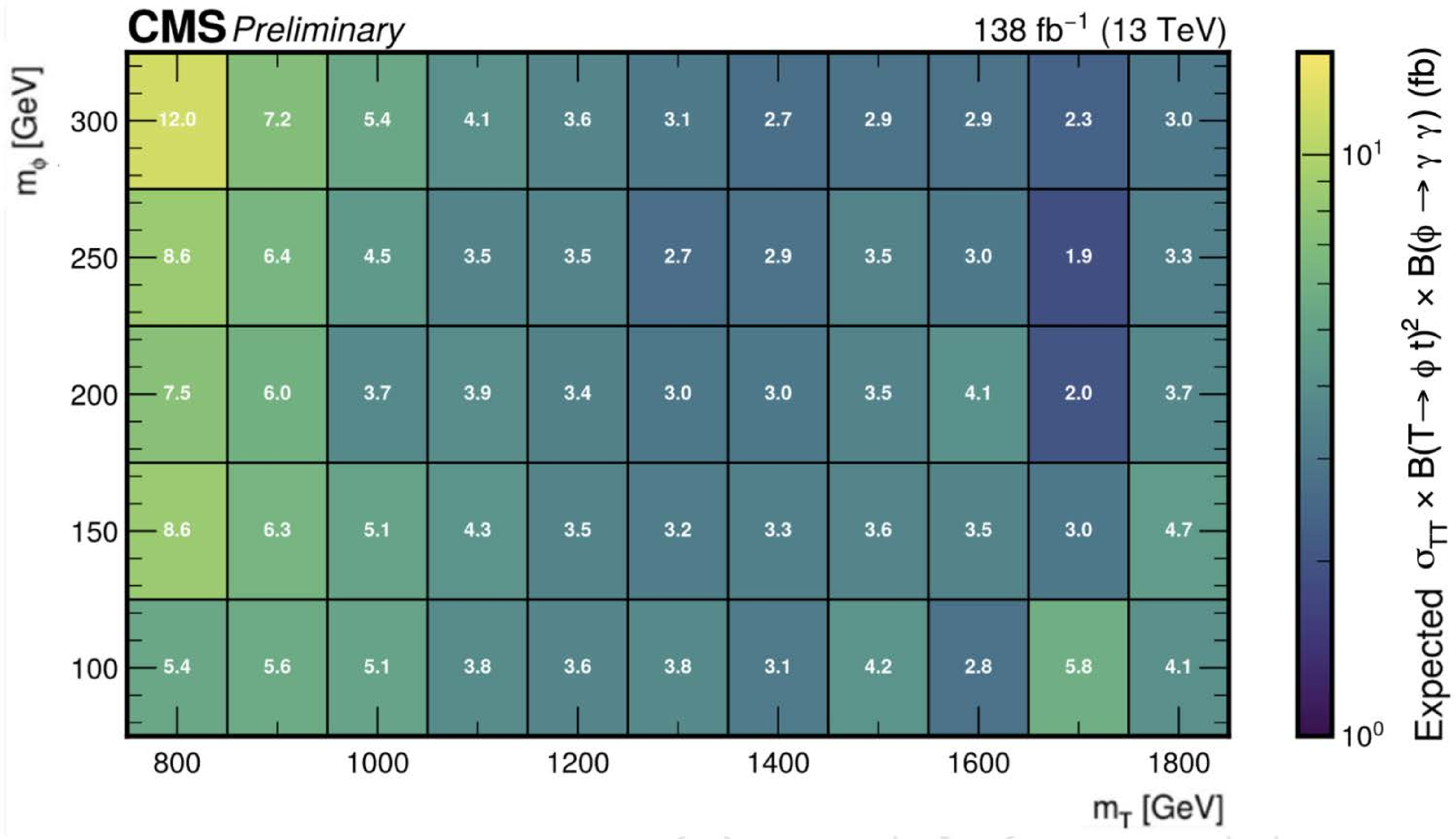
Figure 7:
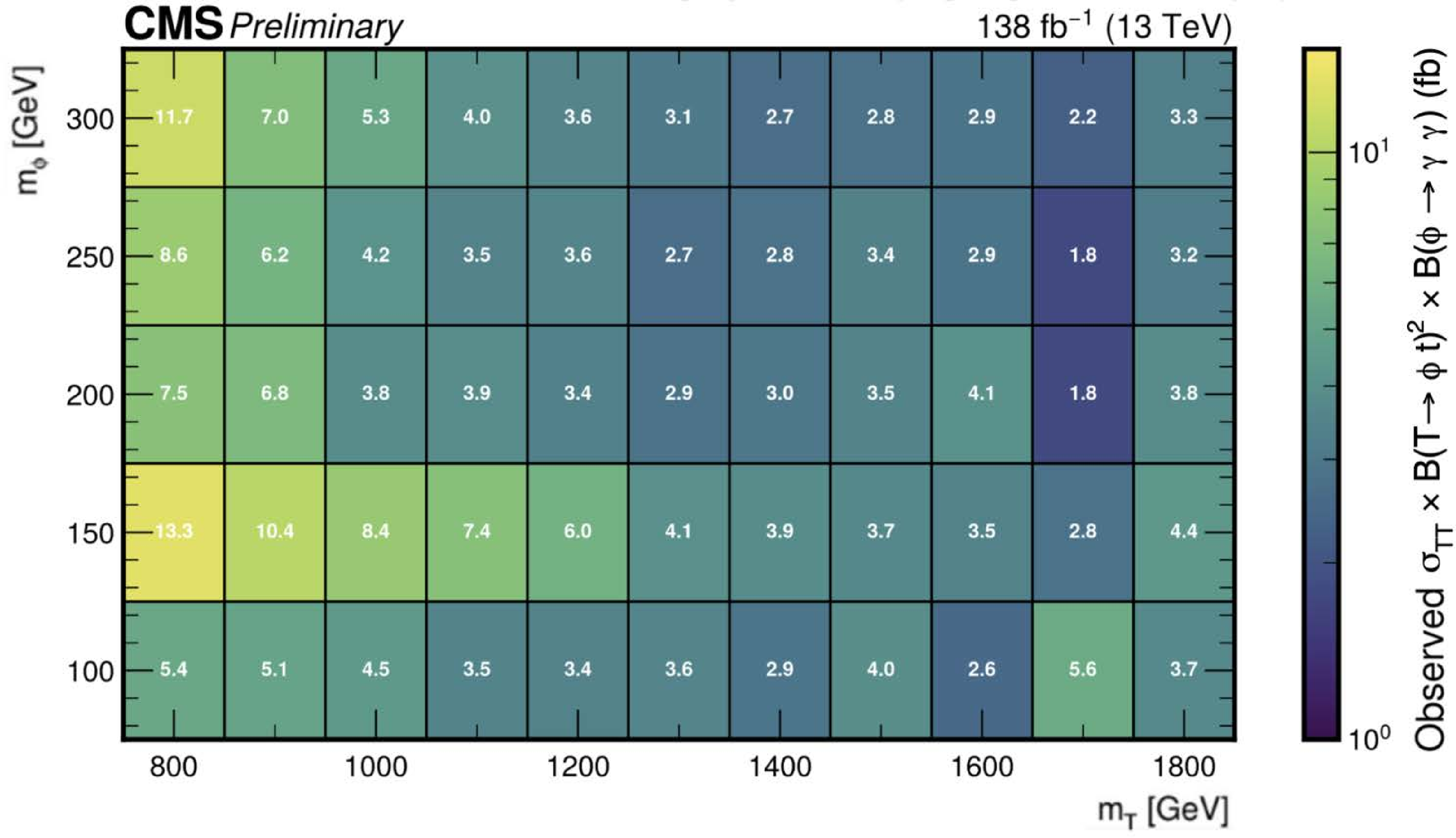
Expected (top) and observed (bottom) upper limits on $ \sigma_{{\mathrm{T}} {\mathrm{T}} } \times B({\mathrm{T}} \to \phi \mathrm{t})^2 \times B(\phi \to \gamma\gamma) $ in the $ (m_{{\mathrm{T}} }, m_{\phi}) $ plane. |
png pdf |
Figure 7-a:
Expected (top) and observed (bottom) upper limits on $ \sigma_{{\mathrm{T}} {\mathrm{T}} } \times B({\mathrm{T}} \to \phi \mathrm{t})^2 \times B(\phi \to \gamma\gamma) $ in the $ (m_{{\mathrm{T}} }, m_{\phi}) $ plane. |
png pdf |
Figure 7-b:
Expected (top) and observed (bottom) upper limits on $ \sigma_{{\mathrm{T}} {\mathrm{T}} } \times B({\mathrm{T}} \to \phi \mathrm{t})^2 \times B(\phi \to \gamma\gamma) $ in the $ (m_{{\mathrm{T}} }, m_{\phi}) $ plane. |
png pdf |
Figure 8:
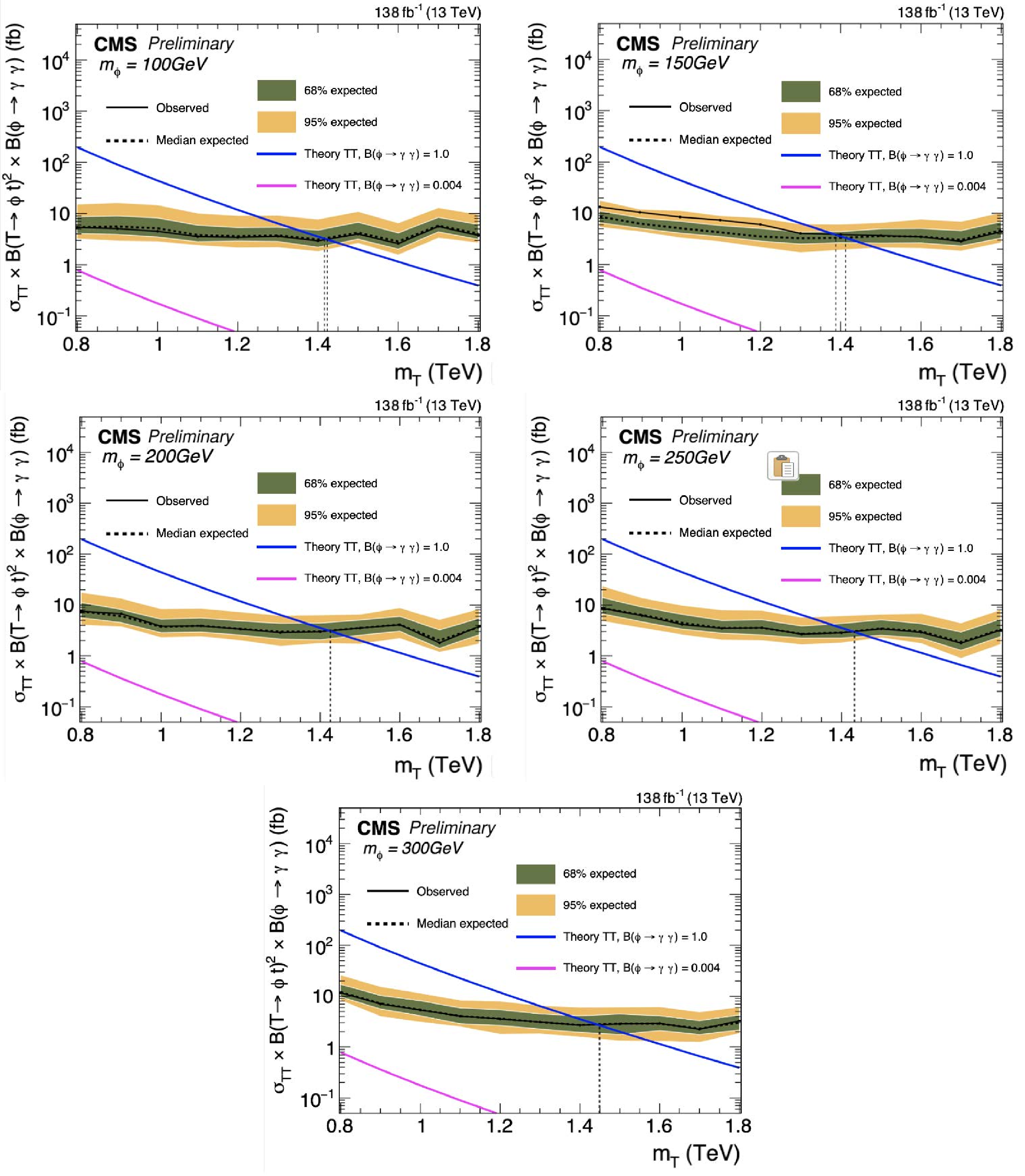
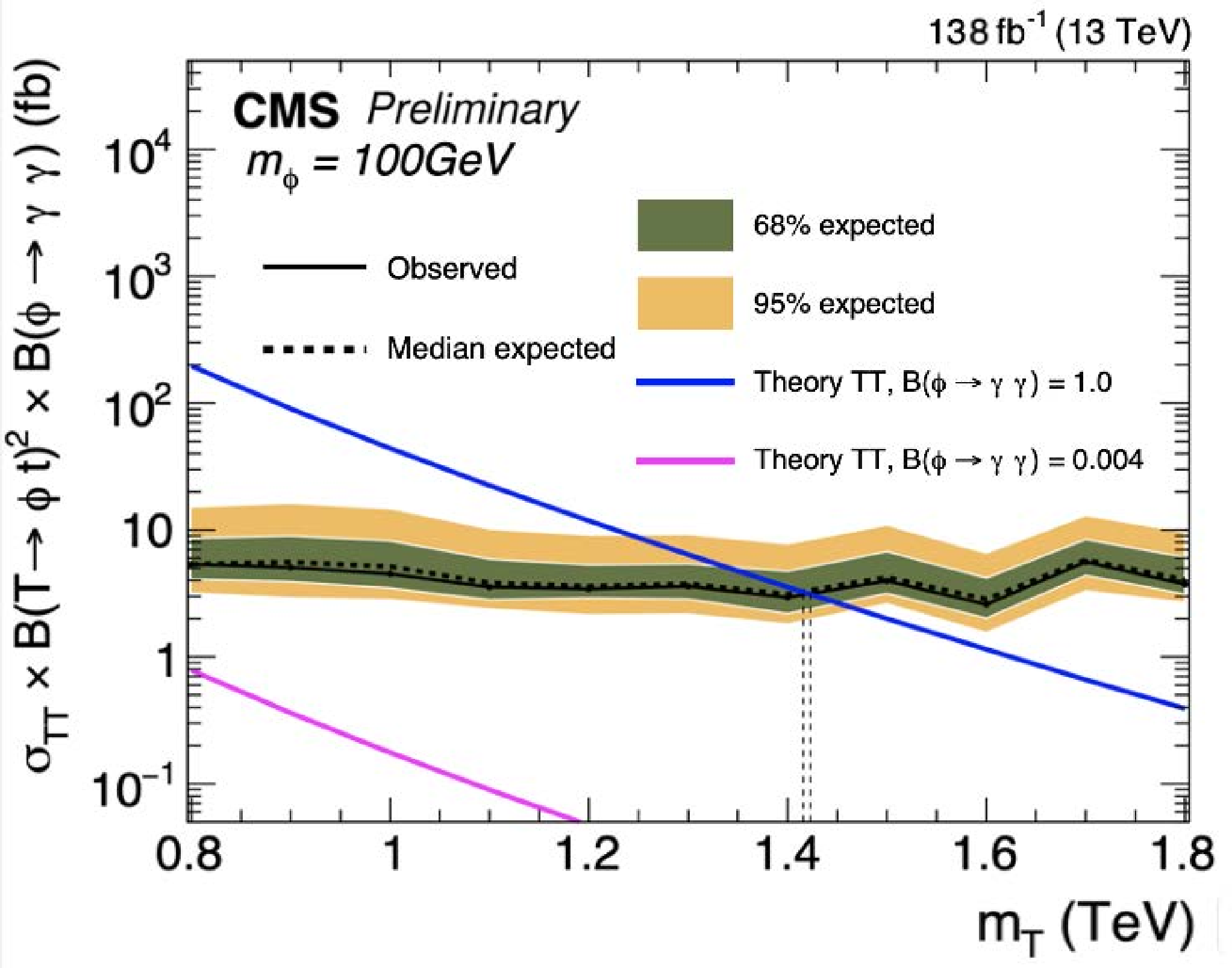
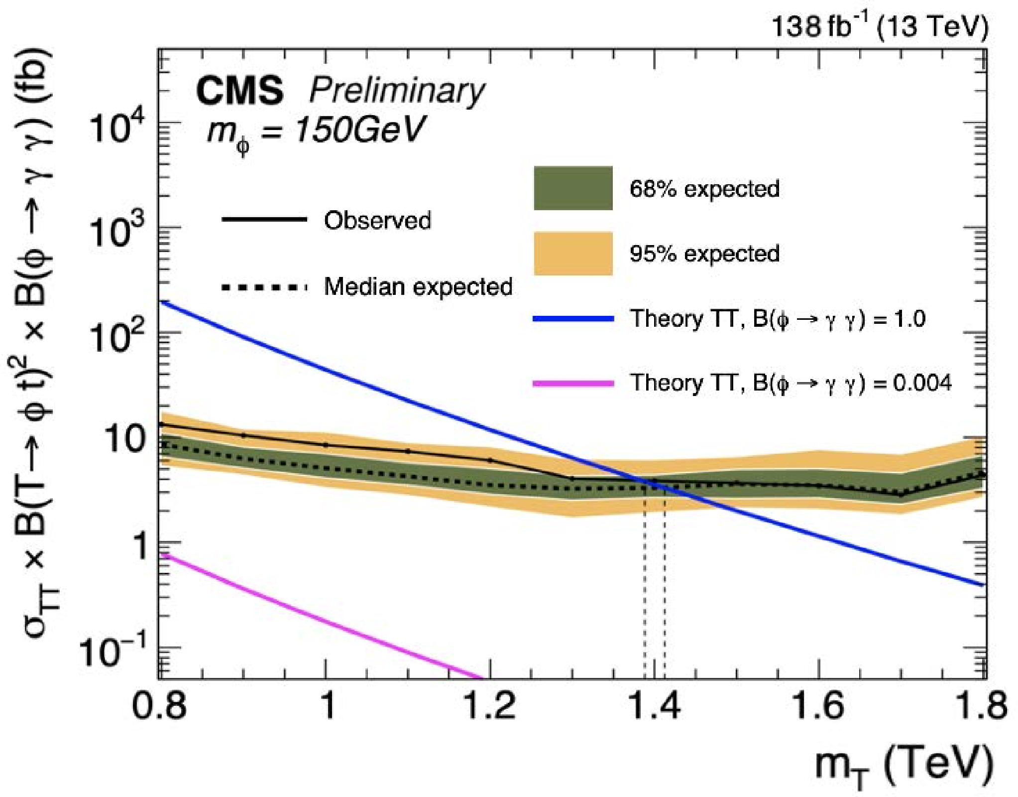
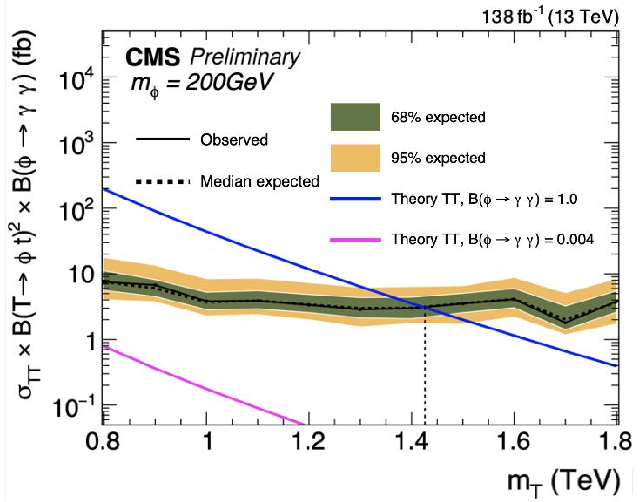
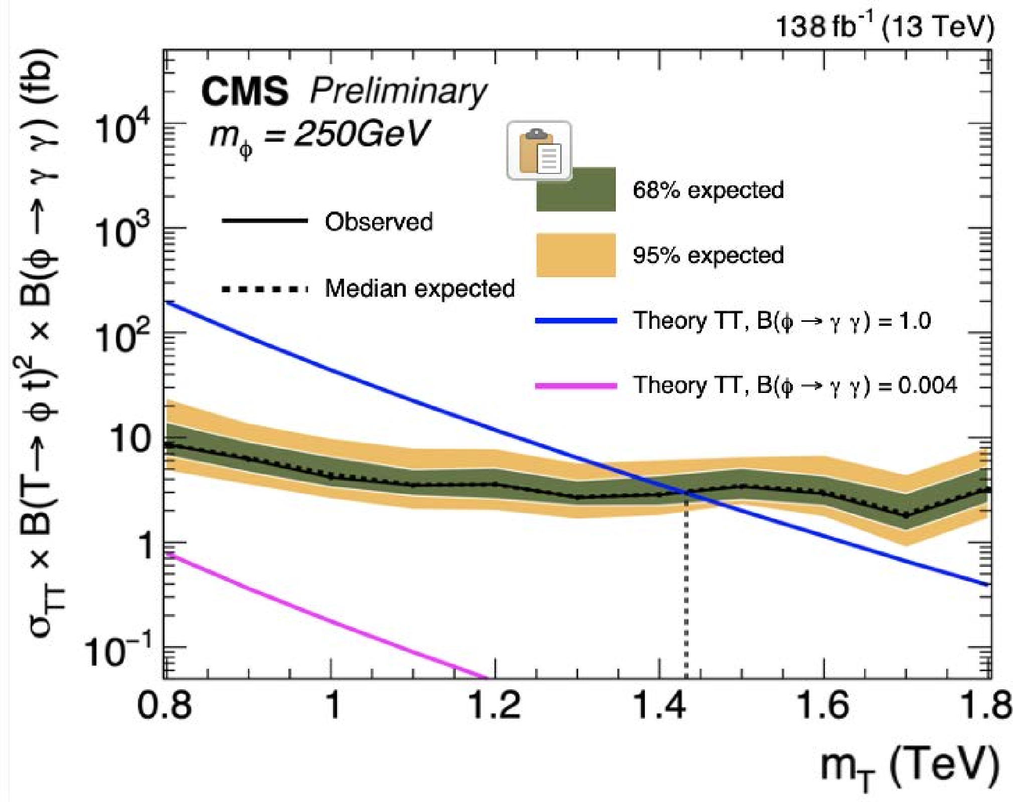
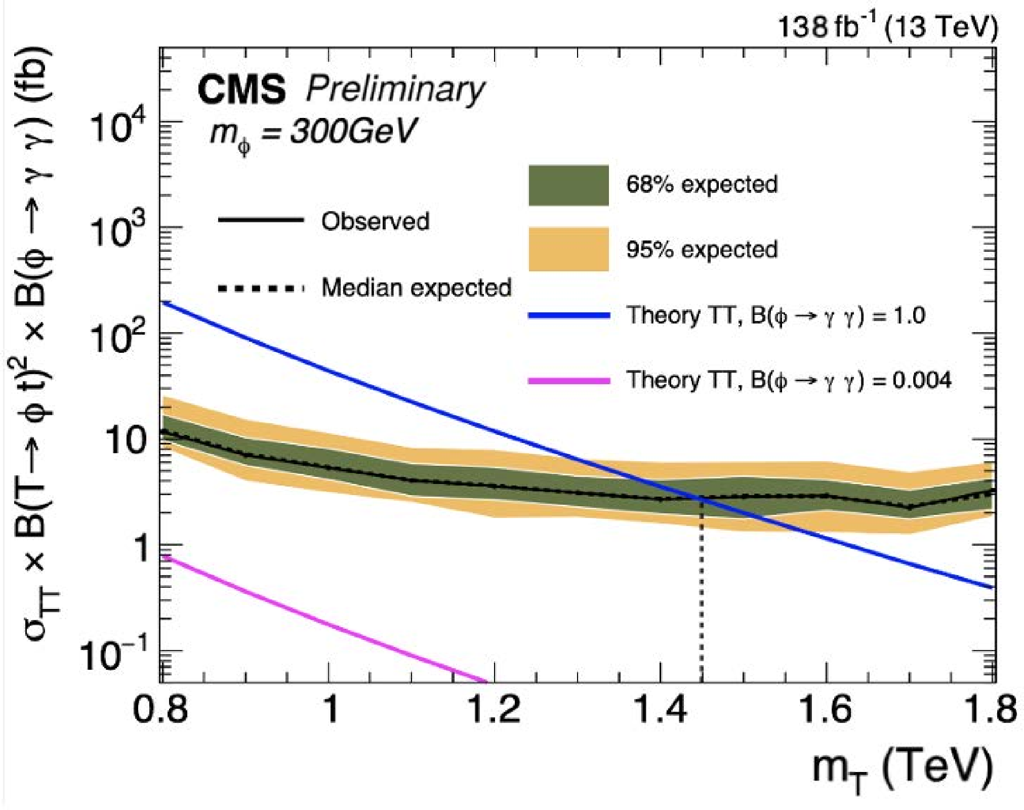
Observed (solid) and expected (dashed) upper limits on the $ {\mathrm{T}} {\mathrm{T}} $ production cross section as a function of $ m_{{\mathrm{T}} } $ for different values of $ m_{\phi} $. The first row shows $ m_{\phi}= $ 100 and 150 GeV (left to right), the second row shows $ m_{\phi}= $ 200 and 250 GeV (left to right), and the third row shows $ m_{\phi}= $ 300 GeV. Theoretical cross section times $ \phi $ branching fractions are shown for $ B(\phi \to \gamma\gamma)= $ 1.0 (blue) and 0.004 (magenta). |
png pdf |
Figure 8-a:
Observed (solid) and expected (dashed) upper limits on the $ {\mathrm{T}} {\mathrm{T}} $ production cross section as a function of $ m_{{\mathrm{T}} } $ for different values of $ m_{\phi} $. The first row shows $ m_{\phi}= $ 100 and 150 GeV (left to right), the second row shows $ m_{\phi}= $ 200 and 250 GeV (left to right), and the third row shows $ m_{\phi}= $ 300 GeV. Theoretical cross section times $ \phi $ branching fractions are shown for $ B(\phi \to \gamma\gamma)= $ 1.0 (blue) and 0.004 (magenta). |
png pdf |
Figure 8-b:
Observed (solid) and expected (dashed) upper limits on the $ {\mathrm{T}} {\mathrm{T}} $ production cross section as a function of $ m_{{\mathrm{T}} } $ for different values of $ m_{\phi} $. The first row shows $ m_{\phi}= $ 100 and 150 GeV (left to right), the second row shows $ m_{\phi}= $ 200 and 250 GeV (left to right), and the third row shows $ m_{\phi}= $ 300 GeV. Theoretical cross section times $ \phi $ branching fractions are shown for $ B(\phi \to \gamma\gamma)= $ 1.0 (blue) and 0.004 (magenta). |
png pdf |
Figure 8-c:
Observed (solid) and expected (dashed) upper limits on the $ {\mathrm{T}} {\mathrm{T}} $ production cross section as a function of $ m_{{\mathrm{T}} } $ for different values of $ m_{\phi} $. The first row shows $ m_{\phi}= $ 100 and 150 GeV (left to right), the second row shows $ m_{\phi}= $ 200 and 250 GeV (left to right), and the third row shows $ m_{\phi}= $ 300 GeV. Theoretical cross section times $ \phi $ branching fractions are shown for $ B(\phi \to \gamma\gamma)= $ 1.0 (blue) and 0.004 (magenta). |
png pdf |
Figure 8-d:
Observed (solid) and expected (dashed) upper limits on the $ {\mathrm{T}} {\mathrm{T}} $ production cross section as a function of $ m_{{\mathrm{T}} } $ for different values of $ m_{\phi} $. The first row shows $ m_{\phi}= $ 100 and 150 GeV (left to right), the second row shows $ m_{\phi}= $ 200 and 250 GeV (left to right), and the third row shows $ m_{\phi}= $ 300 GeV. Theoretical cross section times $ \phi $ branching fractions are shown for $ B(\phi \to \gamma\gamma)= $ 1.0 (blue) and 0.004 (magenta). |
png pdf |
Figure 8-e:
Observed (solid) and expected (dashed) upper limits on the $ {\mathrm{T}} {\mathrm{T}} $ production cross section as a function of $ m_{{\mathrm{T}} } $ for different values of $ m_{\phi} $. The first row shows $ m_{\phi}= $ 100 and 150 GeV (left to right), the second row shows $ m_{\phi}= $ 200 and 250 GeV (left to right), and the third row shows $ m_{\phi}= $ 300 GeV. Theoretical cross section times $ \phi $ branching fractions are shown for $ B(\phi \to \gamma\gamma)= $ 1.0 (blue) and 0.004 (magenta). |
| Tables | |
png pdf |
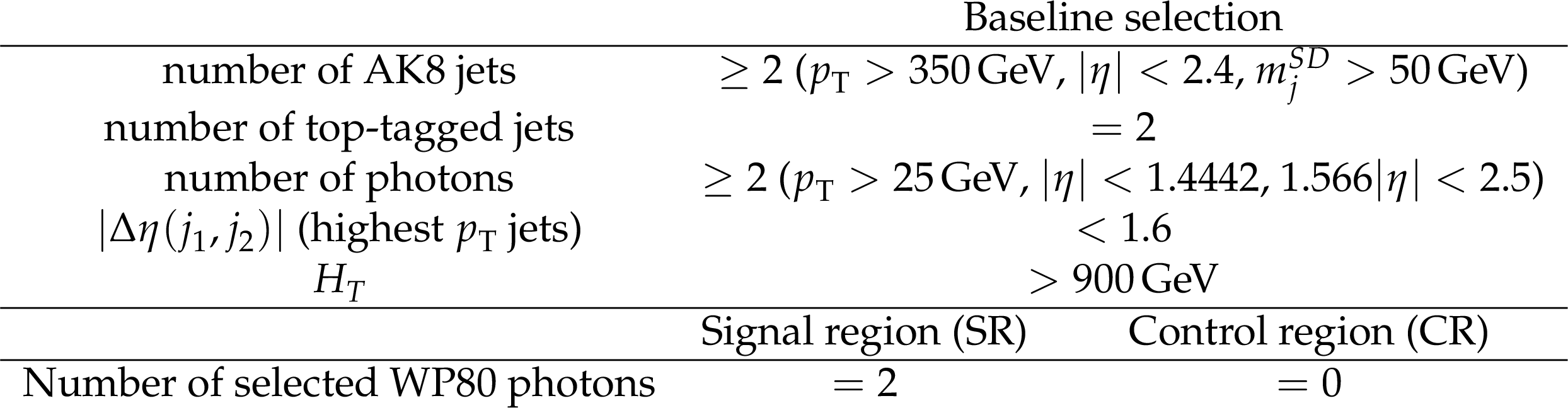
Table 1:
Event selection for the signal and control regions |
png pdf |
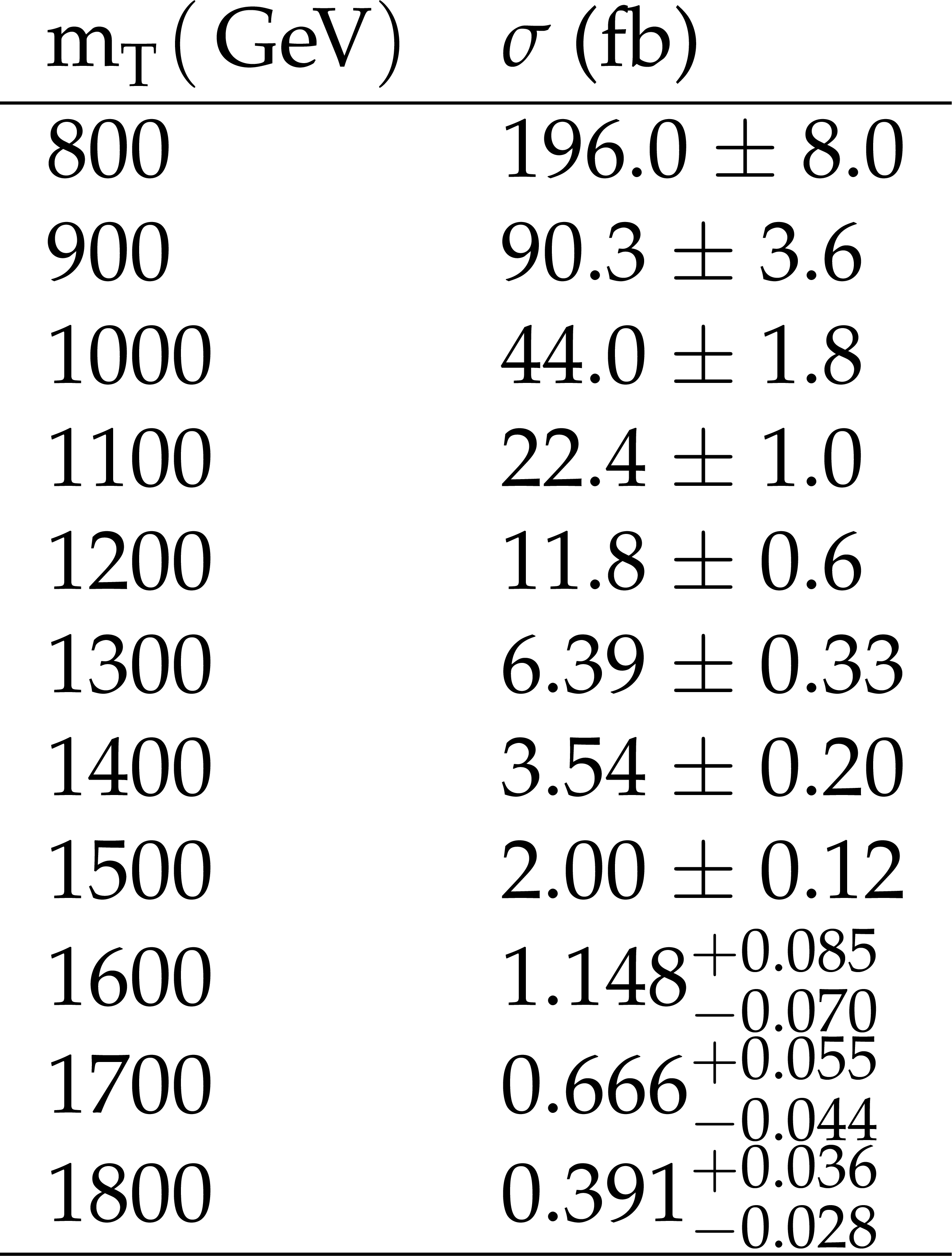
Table 2:
Theoretical NNLO cross sections for {\HepParticleT} pair production [48]. |
| Summary |
| A search for the pair production of vector-like top quarks $ {\mathrm{T}} $ in a scenario involving an additional scalar boson is presented. The search uses proton-proton collision data collected by the CMS experiment at the LHC during 2016--2018, corresponding to an integrated luminosity of 138 fb$ ^{-1} $. The analysis considers $ {\mathrm{T}} {\mathrm{T}} $ production, with each $ {\mathrm{T}} $ decaying to a standard model top quark and a scalar boson $ \phi $. The top quarks are required to decay hadronically, and one of the scalar bosons is required to decay to a pair of photons, while the second $ \phi $ boson is treated inclusively. The top quarks are reconstructed as large-radius jets and identified using a ParticleNet discriminant, while a multivariate discriminant is used for photon identification. A data-driven method is used to predict the background in the signal region from the $ \mathrm{t}\overline{\mathrm{t}} $ distribution in a control region via a transfer function. No significant deviation from the background prediction is observed. Assuming a branching fraction $ B(\phi \to \gamma\gamma)=100% $, vector-like top quark masses below 1.39 TeV are excluded. |
| References | ||||
| 1 | CMS Collaboration | Observation of a new boson at a mass of 125 GeV with the CMS experiment at the LHC | PLB 716 (2012) 30 | CMS-HIG-12-028 1207.7235 |
| 2 | ATLAS Collaboration | Observation of a new particle in the search for the Standard Model Higgs boson with the ATLAS detector at the LHC | PLB 716 (2012) 1 | 1207.7214 |
| 3 | M. E. Peskin | What is the hierarchy problem? | NPB 1018 (2025) 116971 | |
| 4 | B. Guo, Y.-X. Liu, K. Yang, and S.-W. Wei | Hierarchy problem and new warped extra dimension | PRD 98 (2018) 085022 | 1805.03976 |
| 5 | G. F. Giudice, C. Grojean, A. Pomarol, and R. Rattazzi | The strongly-interacting light Higgs | JHEP 06 (2007) 045 | hep-ph/0703164 |
| 6 | P. Lodone | Vector-like quarks in a 'composite' Higgs model | JHEP 12 (2008) 029 | 0806.1472 |
| 7 | R. Benbrik et al. | Signatures of vector-like top partners decaying into new neutral scalar or pseudoscalar bosons | JHEP 05 (2020) 028 | 1907.05929 |
| 8 | R. Benbrik et al. | Vector-like quarks at the LHC: A unified perspective from ATLAS and CMS exclusion limits | JHEP 03 (2025) 020 | |
| 9 | ATLAS Collaboration | Exploration at the high-energy frontier: ATLAS Run 2 searches investigating the exotic jungle beyond the Standard Model | Phys. Rept. 1116 (2025) 301 | 2403.09292 |
| 10 | CMS Collaboration | Review of searches for vector-like quarks, vector-like leptons, and heavy neutral leptons in proton-proton collisions at \ensuremath\sqrts=13 TeV at the CMS experiment | Phys. Rept. 1115 (2025) 570 | CMS-EXO-23-006 2405.17605 |
| 11 | H. Qu and L. Gouskos | ParticleNet: Jet tagging via particle clouds | PRD 101 (2020) 056019 | 1902.08570 |
| 12 | CMS Collaboration | The CMS experiment at the CERN LHC | JINST 3 (2008) S08004 | |
| 13 | CMS Collaboration | Development of the CMS detector for the CERN LHC Run 3 | JINST 19 (2024) P05064 | |
| 14 | CMS Collaboration | Performance of the CMS Level-1 trigger in proton-proton collisions at $ \sqrt{s} = $ 13 TeV | JINST 15 (2020) P10017 | CMS-TRG-17-001 2006.10165 |
| 15 | CMS Collaboration | The CMS trigger system | JINST 12 (2017) P01020 | CMS-TRG-12-001 1609.02366 |
| 16 | CMS Collaboration | Performance of the CMS high-level trigger during LHC Run 2 | JINST 19 (2024) P11021 | CMS-TRG-19-001 2410.17038 |
| 17 | CMS Collaboration | Electron and photon reconstruction and identification with the CMS experiment at the CERN LHC | JINST 16 (2021) P05014 | CMS-EGM-17-001 2012.06888 |
| 18 | CMS Collaboration | Performance of the CMS muon detector and muon reconstruction with proton-proton collisions at $ \sqrt{s}= $ 13 TeV | JINST 13 (2018) P06015 | CMS-MUO-16-001 1804.04528 |
| 19 | CMS Collaboration | Description and performance of track and primary-vertex reconstruction with the CMS tracker | JINST 9 (2014) P10009 | CMS-TRK-11-001 1405.6569 |
| 20 | CMS Collaboration | Particle-flow reconstruction and global event description with the CMS detector | JINST 12 (2017) P10003 | CMS-PRF-14-001 1706.04965 |
| 21 | A. Hoecker et al. | TMVA: Toolkit for Multivariate Data Analysis | PoS ACAT 04 (2007) 0 | physics/0703039 |
| 22 | CMS Collaboration | Performance of photon reconstruction and identification with the CMS detector in proton-proton collisions at sqrt(s) = 8 TeV | JINST 10 (2015) P08010 | CMS-EGM-14-001 1502.02702 |
| 23 | CMS Collaboration | A measurement of the Higgs boson mass in the diphoton decay channel | PLB 805 (2020) 135425 | CMS-HIG-19-004 2002.06398 |
| 24 | M. Cacciari, G. P. Salam, and G. Soyez | The anti-$ k_{\mathrm{T}} $ jet clustering algorithm | JHEP 04 (2008) 063 | 0802.1189 |
| 25 | M. Cacciari, G. P. Salam, and G. Soyez | FastJet user manual | EPJC 72 (2012) 1896 | 1111.6097 |
| 26 | CMS Collaboration | Jet energy scale and resolution in the CMS experiment in pp collisions at 8 TeV | JINST 12 (2017) P02014 | CMS-JME-13-004 1607.03663 |
| 27 | M. Dasgupta, A. Fregoso, S. Marzani, and G. P. Salam | Towards an understanding of jet substructure | JHEP 09 (2013) 029 | 1307.0007 |
| 28 | J. M. Butterworth, A. R. Davison, M. Rubin, and G. P. Salam | Jet substructure as a new Higgs search channel at the LHC | PRL 100 (2008) 242001 | 0802.2470 |
| 29 | A. J. Larkoski, S. Marzani, G. Soyez, and J. Thaler | Soft drop | JHEP 05 (2014) 146 | 1402.2657 |
| 30 | CMS Collaboration | Pileup mitigation at CMS in 13 TeV data | JINST 15 (2020) P09018 | CMS-JME-18-001 2003.00503 |
| 31 | J. Alwall et al. | MadGraph 5: Going Beyond | JHEP 06 (2011) 128 | 1106.0522 |
| 32 | A. Banerjee et al. | Phenomenological aspects of composite Higgs scenarios: Exotic scalars and vector-like quarks | ||
| 33 | S. Frixione, P. Nason, and C. Oleari | Matching NLO QCD computations with Parton Shower simulations: the POWHEG method | JHEP 11 (2007) 070 | 0709.2092 |
| 34 | R. D. Ball et al. | Parton distributions from high-precision collider data | EPJC 77 (2017) 663 | 1706.00428 |
| 35 | T. Sjostrand et al. | An introduction to PYTHIA 8.2 | Comput. Phys. Commun. 191 (2015) 159 | 1410.3012 |
| 36 | CMS Collaboration | Extraction and validation of a new set of CMS PYTHIA8 tunes from underlying-event measurements | EPJC 80 (2020) 4 | CMS-GEN-17-001 1903.12179 |
| 37 | GEANT4 Collaboration | GEANT 4---a simulation toolkit | NIM A 506 (2003) 250 | |
| 38 | CMS Collaboration | The CMS statistical analysis and combination tool: COMBINE | Comput. Softw. Big Sci. 8 (2024) 19 | CMS-CAT-23-001 2404.06614 |
| 39 | CMS Collaboration | Precision luminosity measurement in proton-proton collisions at $ \sqrt{s} = $ 13 TeV in 2015 and 2016 at CMS | EPJC 81 (2021) 800 | CMS-LUM-17-003 2104.01927 |
| 40 | CMS Collaboration | Precision luminosity measurement in proton-proton collisions at 13 tev with the CMS detector | CMS Physics Analysis Summary, 2025 CMS-PAS-LUM-20-001 |
CMS-PAS-LUM-20-001 |
| 41 | J. Butterworth et al. | PDF4LHC recommendations for LHC Run II | JPG 43 (2016) 023001 | 1510.03865 |
| 42 | CMS Collaboration | Search for narrow H$ \gamma $ resonances in proton-proton collisions at $ \sqrt{s} = $ 13 TeV | PRL 122 (2019) 081804 | 1812.06518 |
| 43 | A. L. Read | Presentation of search results: The CL$ _{\text{s}} $ technique | JPG 28 (2002) 2693 | |
| 44 | T. Junk | Confidence level computation for combining searches with small statistics | NIM A 434 (1999) 435 | hep-ex/9902006 |
| 45 | W. Verkerke and D. Kirkby | The RooFit toolkit for data modeling | in the Int. Conf. on Computing in High Energy and Nuclear Physics (CHEP ), La Jolla, CA, March 24--28, 2003 Proc. 1 (2003) 3 |
physics/0306116 |
| 46 | L. Moneta et al. | The RooStats project | in the Int. Workshop on Advanced Computing and Analysis Techniques in Physics Research (ACAT ), Jaipur, India, February 22--27, 2010 Proc. 1 (2010) 3 |
1009.1003 |
| 47 | Particle Data Group Collaboration | Review of particle physics | PRD 110 (2024) 030001 | |
| 48 | M. Czakon and A. Mitov | Top++: A Program for the Calculation of the Top-Pair Cross-Section at Hadron Colliders | Comput. Phys. Commun. 185 (2014) 2930 | 1112.5675 |
| 49 | M. Czakon, P. Fiedler, and A. Mitov | Total top-quark pair-production cross section at hadron colliders | PRL 110 (2013) 252004 | 1303.6254 |
|
|
Compact Muon Solenoid LHC, CERN |
|

|

|

|

|

|