

Compact Muon Solenoid
LHC, CERN
| CMS-PAS-TOP-17-005 | ||
| Measurement of top quark pair-production in association with a W or Z boson in pp collisions at 13 TeV | ||
| CMS Collaboration | ||
| May 2017 | ||
| Abstract: We present a measurement of the cross section of top quark pair production in association with a W or Z boson, in proton-proton collisions at a center-of-mass energy of 13 TeV at the LHC. The data sample used corresponds to an integrated luminosity of 35.9 fb$^{-1}$, collected in 2016 by the CMS experiment. The measurement is performed in same-charge dilepton, three- and four-lepton final states where the jet and b-jet multiplicities are exploited to enhance the signal-to-background ratio. The $\mathrm{t\overline{t}W}$ and $\mathrm{t\overline{t}Z}$ production cross sections are measured to be $\sigma(\mathrm{t\overline{t}W})= $ 0.80$^{+0.12}_{-0.11}$ (stat.) $^{+0.13}_{-0.12}$ (sys.) pb and $\sigma(\mathrm{t\overline{t}Z})= $ 1.00$^{+0.09}_{-0.08}$ (stat.) $^{+0.12}_{-0.10}$ (sys.) pb with an expected (observed) significance of 4.6 (5.5) and 9.5 (9.9) standard deviations from the background-only hypothesis respectively. The measured cross sections are in agreement with the standard model prediction. We use these measurements to constrain the Wilson coefficients for four dimension-six operators which would modify $\mathrm{t\overline{t}Z}$ and $\mathrm{t\overline{t}W}$ production. | ||
|
Links:
CDS record (PDF) ;
CADI line (restricted) ;
These preliminary results are superseded in this paper, JHEP 08 (2018) 011. The superseded preliminary plots can be found here. |
||
| Figures | |
png pdf |
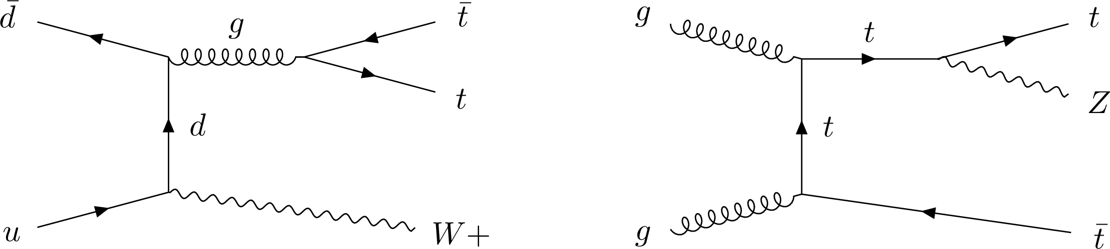
Figure 1:
The leading order Feynman diagram for $ {{\mathrm{ t } {}\mathrm{ \bar{t} } } \mathrm{ Z } } $, $ {{\mathrm{ t } {}\mathrm{ \bar{t} } } \mathrm{ W } } $ production at the LHC. The charge conjugate of the diagrams shown is implied. |
png pdf |
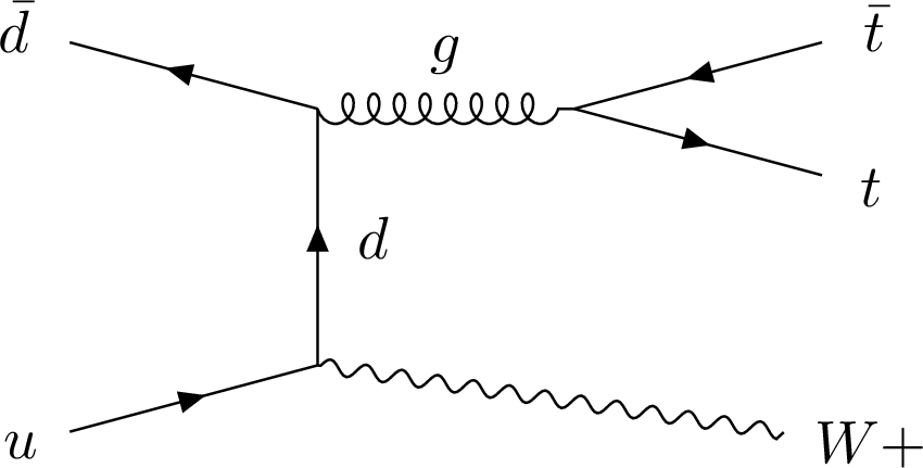
Figure 1-a:
The leading order Feynman diagram for $ {{\mathrm{ t } {}\mathrm{ \bar{t} } } \mathrm{ W } } $ production at the LHC. The charge conjugate of the diagram shown is implied. |
png pdf |
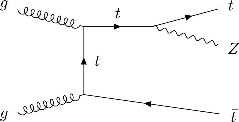
Figure 1-b:
The leading order Feynman diagram for $ {{\mathrm{ t } {}\mathrm{ \bar{t} } } \mathrm{ Z } } $ production at the LHC. The charge conjugate of the diagram shown is implied. |
png pdf |
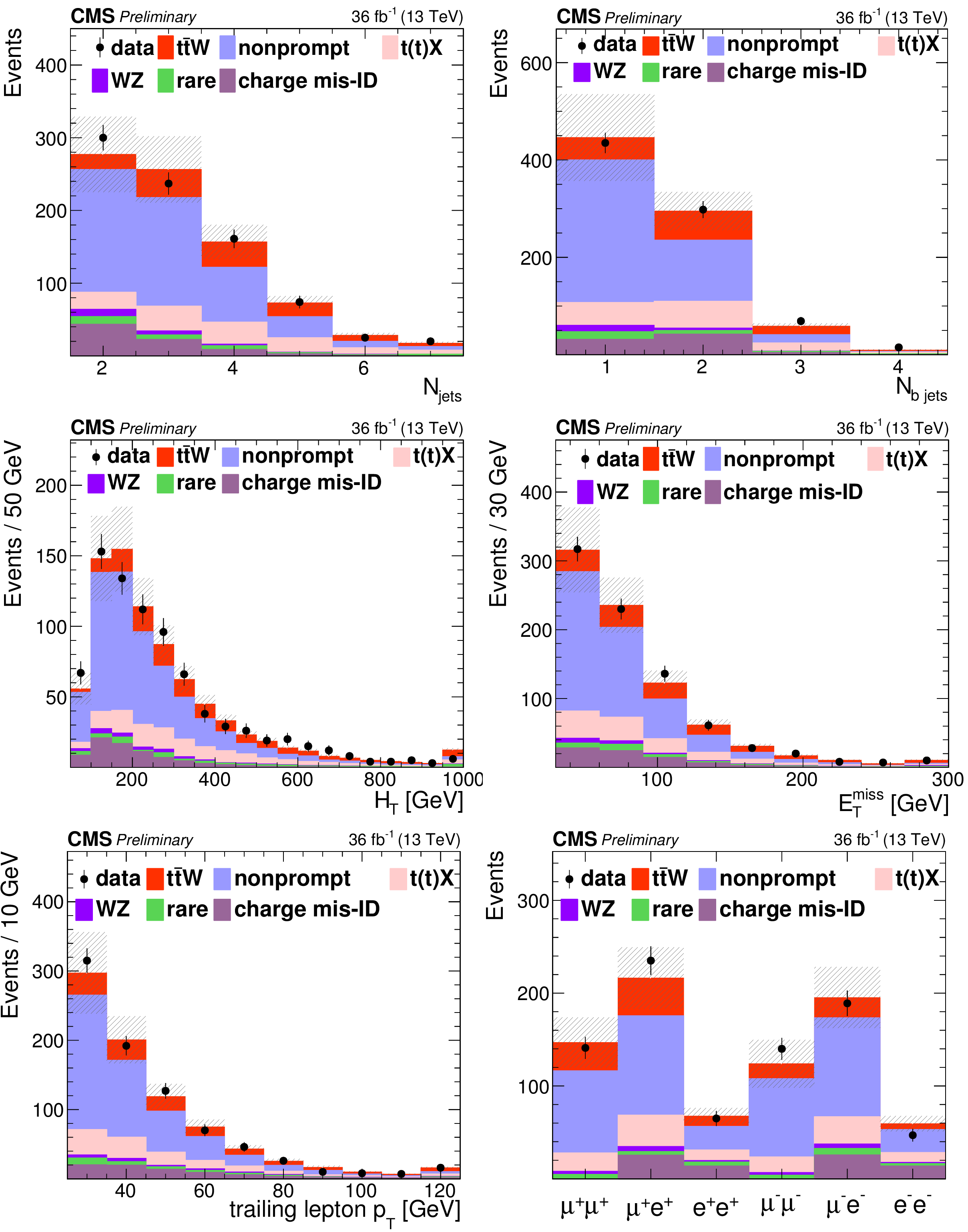
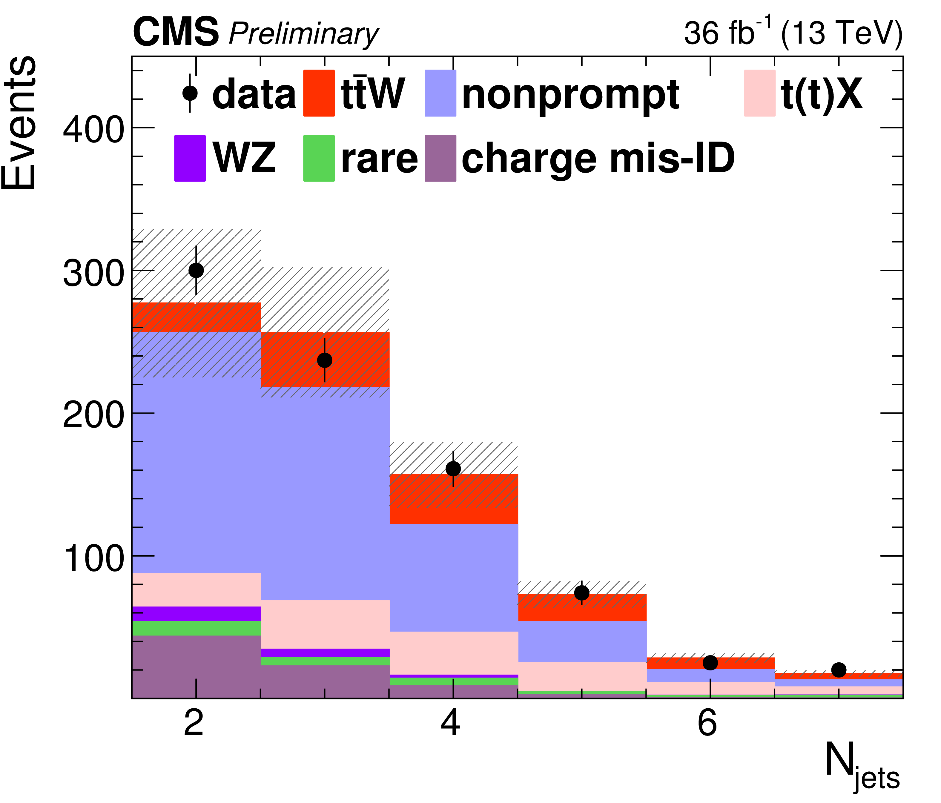
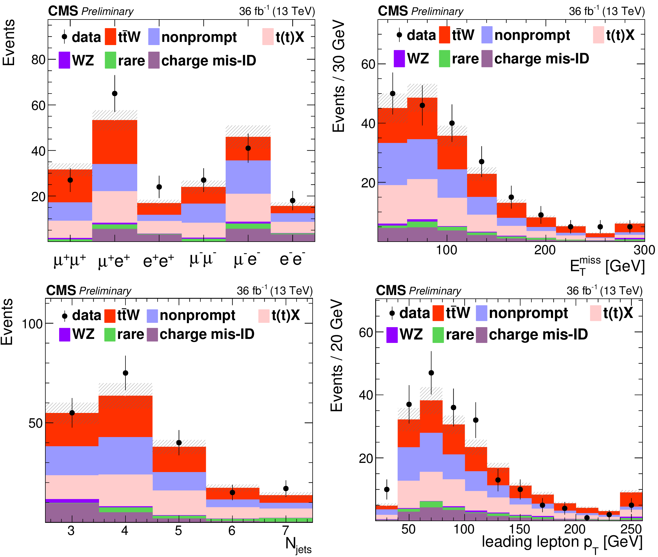
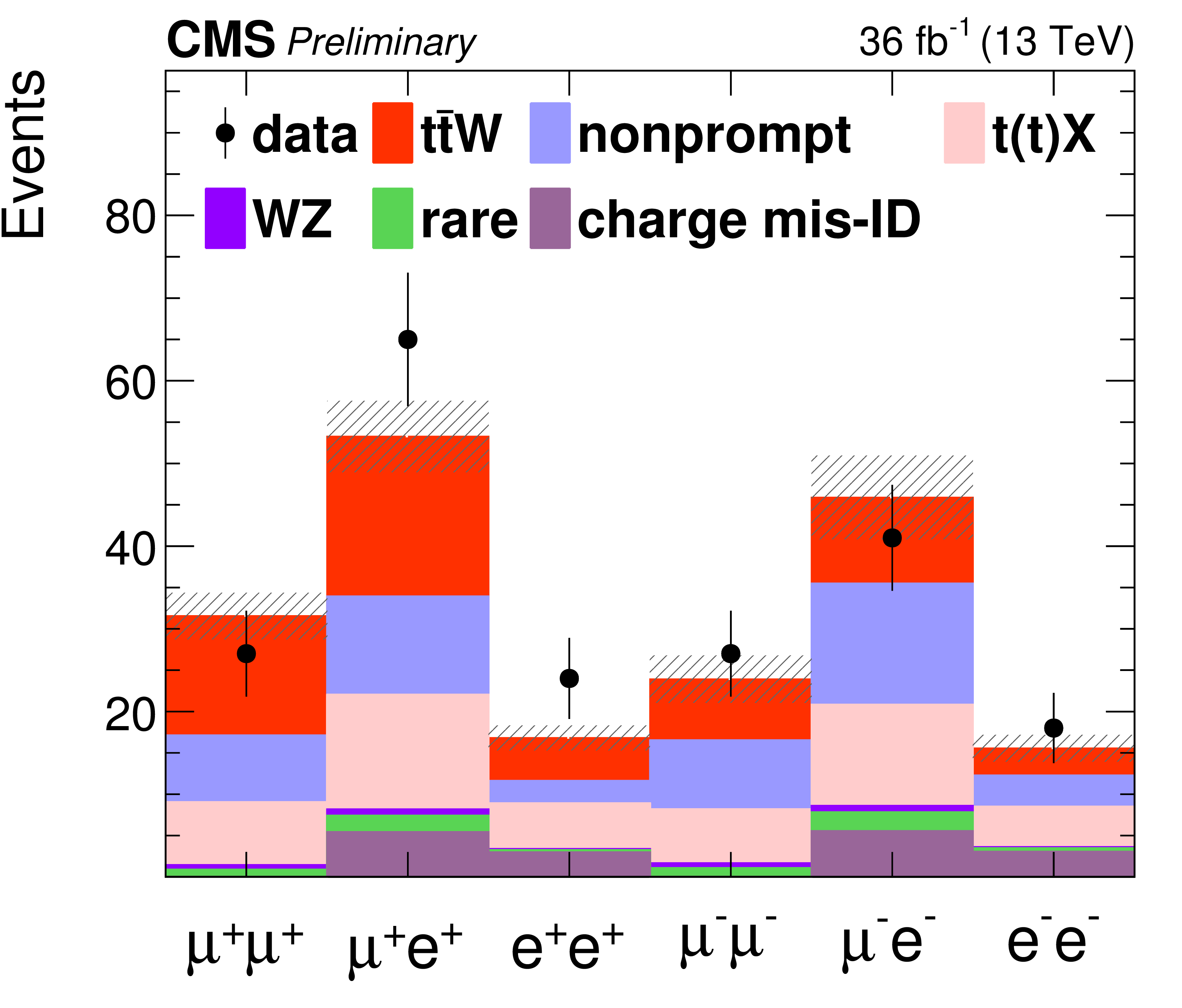
Figure 2:
Distribution of different kinematic variables in data compared to the estimated expectations. From left to right: jet multplicity and b-jet multiplicity (top), ${H_{\mathrm {T}}}$ and ${E_{\mathrm {T}}^{\text {miss}}}$ (center), trailing lepton ${p_{\mathrm {T}}}$ and event yields (bottom). The expected contribution from the different background processes are stacked as well as the expected contribution from the signal. The shaded band represents the uncertainty in the prediction of the background and the signal processes. |
png pdf |
Figure 2-a:
Distribution of Jet multplicity in data compared to the estimated expectation. The expected contribution from the different background processes are stacked as well as the expected contribution from the signal. The shaded band represents the uncertainty in the prediction of the background and the signal processes. |
png pdf |
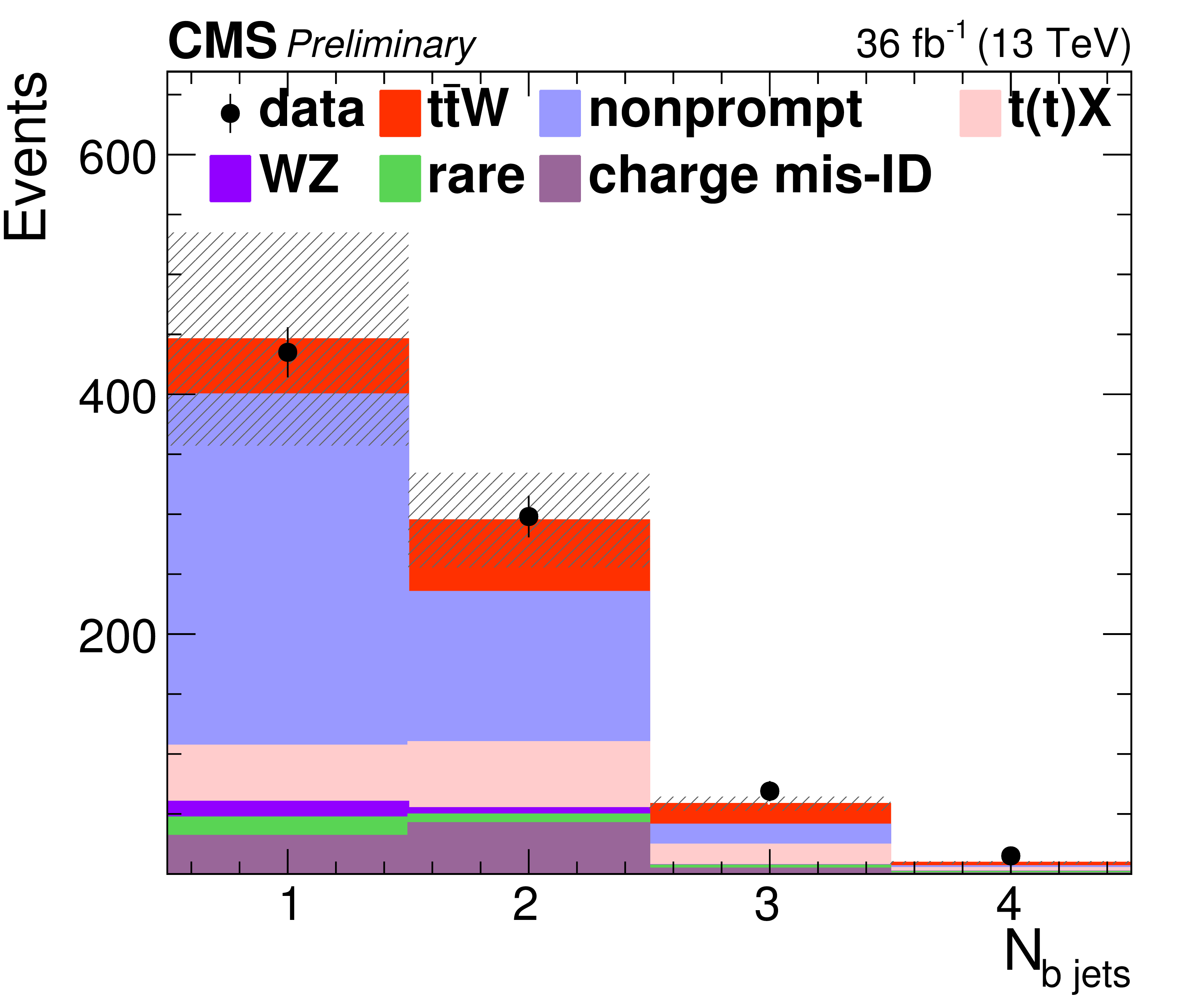
Figure 2-b:
Distribution of b-jet multiplicity in data compared to the estimated expectation. The expected contribution from the different background processes are stacked as well as the expected contribution from the signal. The shaded band represents the uncertainty in the prediction of the background and the signal processes. |
png pdf |
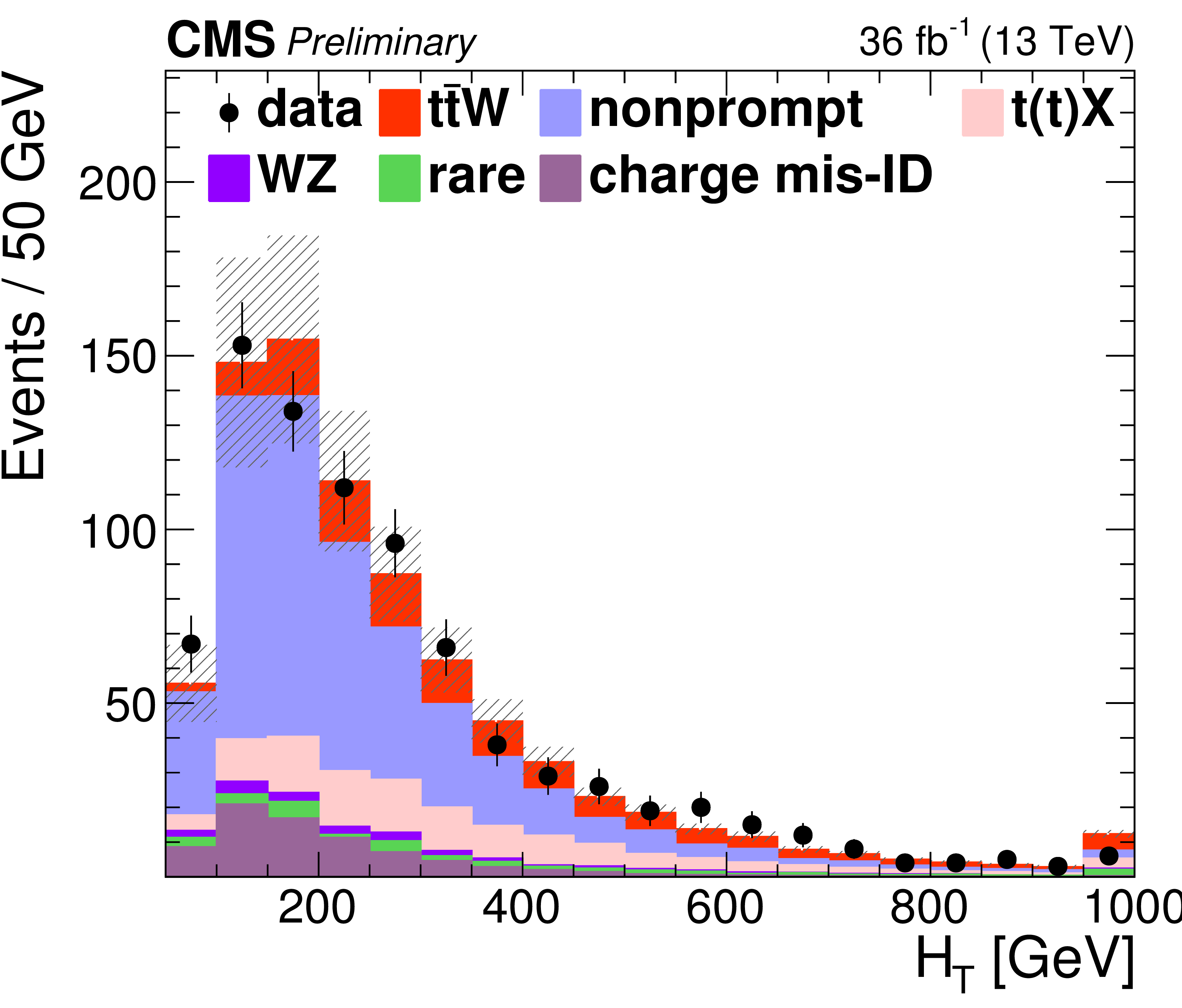
Figure 2-c:
Distribution of ${H_{\mathrm {T}}}$ in data compared to the estimated expectation. The expected contribution from the different background processes are stacked as well as the expected contribution from the signal. The shaded band represents the uncertainty in the prediction of the background and the signal processes. |
png pdf |
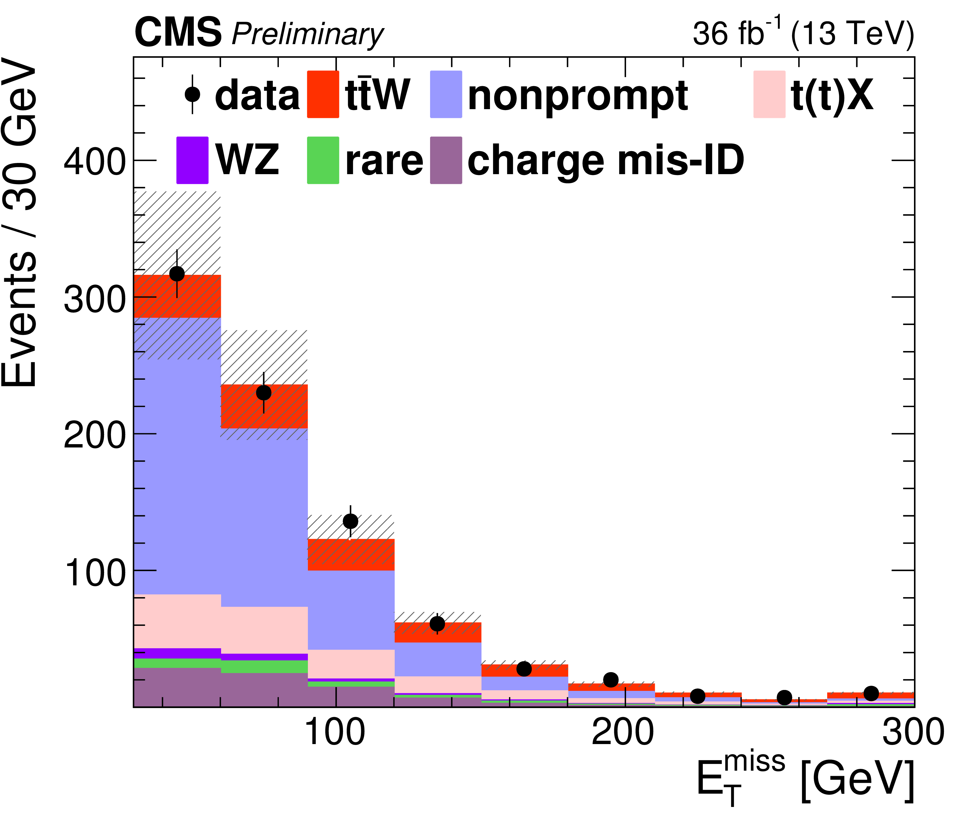
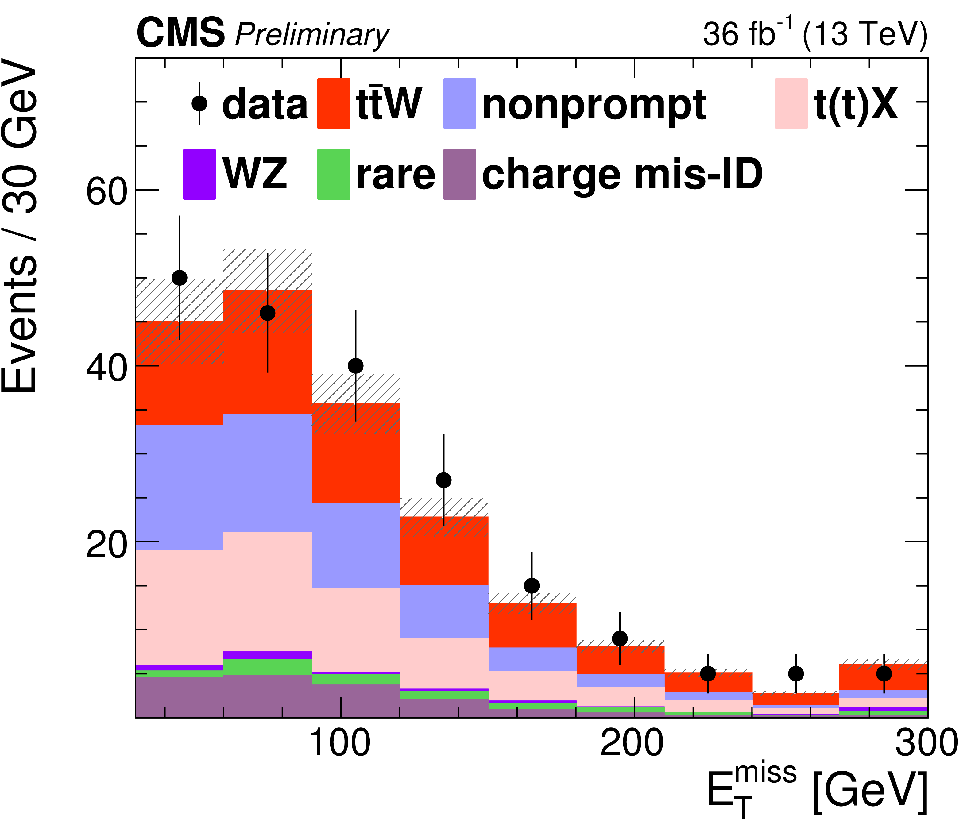
Figure 2-d:
Distribution of ${E_{\mathrm {T}}^{\text {miss}}}$ in data compared to the estimated expectation. The expected contribution from the different background processes are stacked as well as the expected contribution from the signal. The shaded band represents the uncertainty in the prediction of the background and the signal processes. |

png pdf |
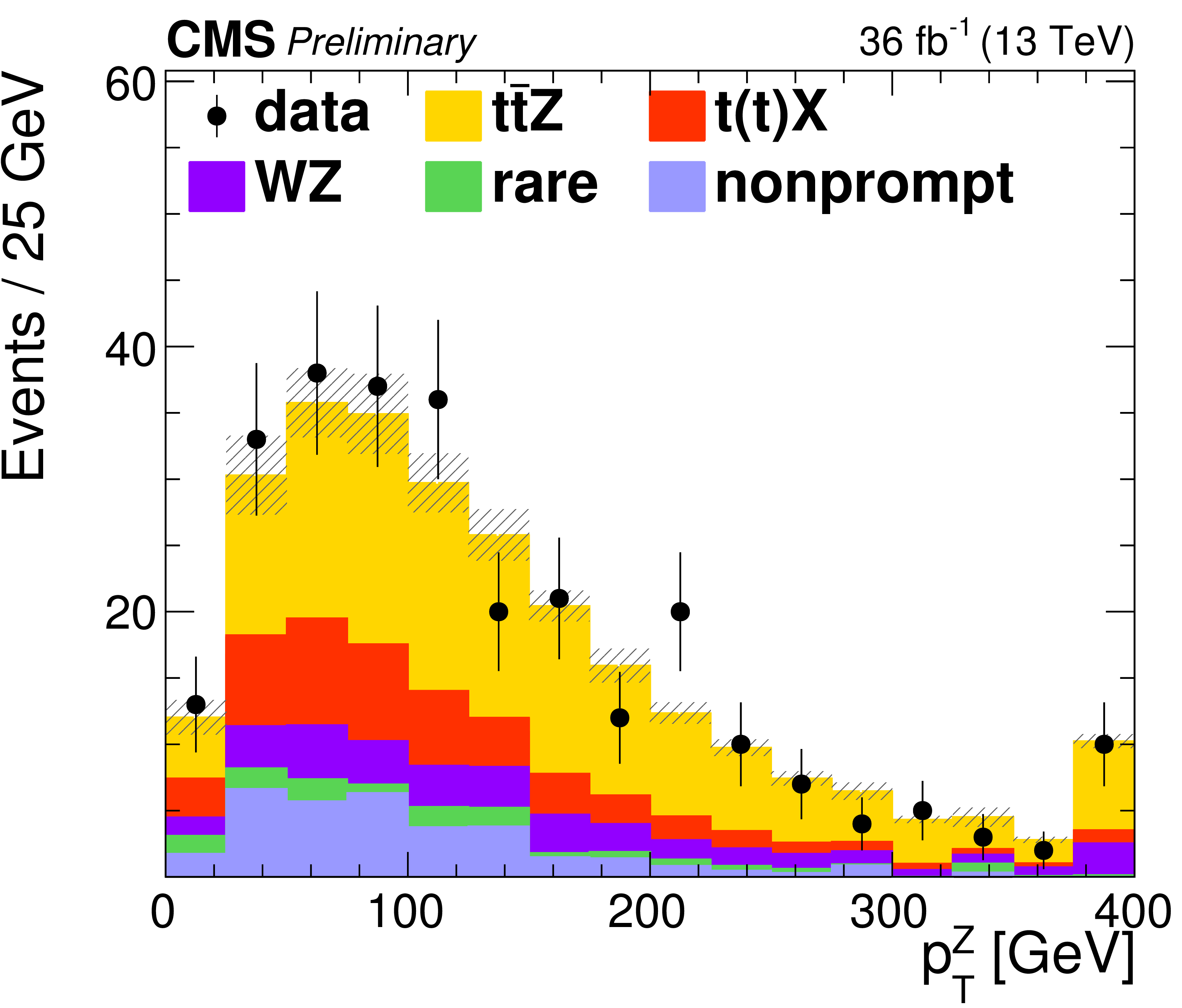
Figure 2-e:
Distribution of trailing lepton ${p_{\mathrm {T}}}$ in data compared to the estimated expectation. The expected contribution from the different background processes are stacked as well as the expected contribution from the signal. The shaded band represents the uncertainty in the prediction of the background and the signal processes. |
png pdf |
Figure 2-f:
Distribution of event yields in data compared to the estimated expectation. The expected contribution from the different background processes are stacked as well as the expected contribution from the signal. The shaded band represents the uncertainty in the prediction of the background and the signal processes. |
png pdf |
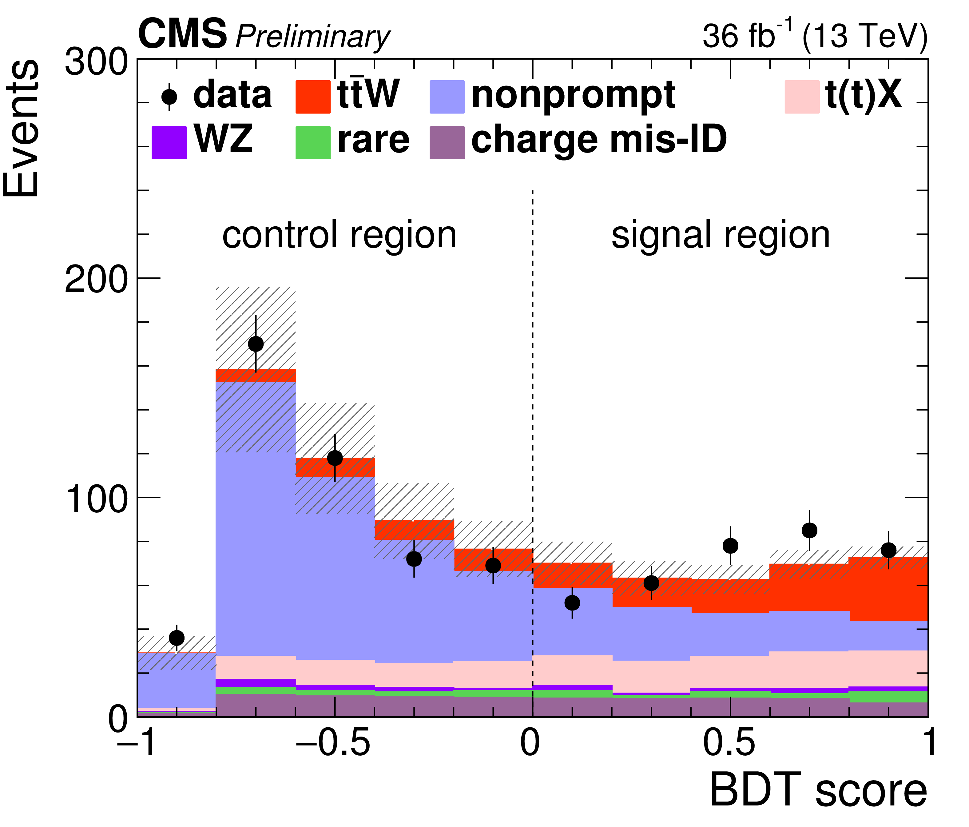
Figure 3:
BDT value distribution for background and signal processes. The expected contribution from the different background processes are stacked as well as the expected contribution from the signal. The shaded band represents the uncertainty in the prediction of the background and the signal processes. |
png pdf |
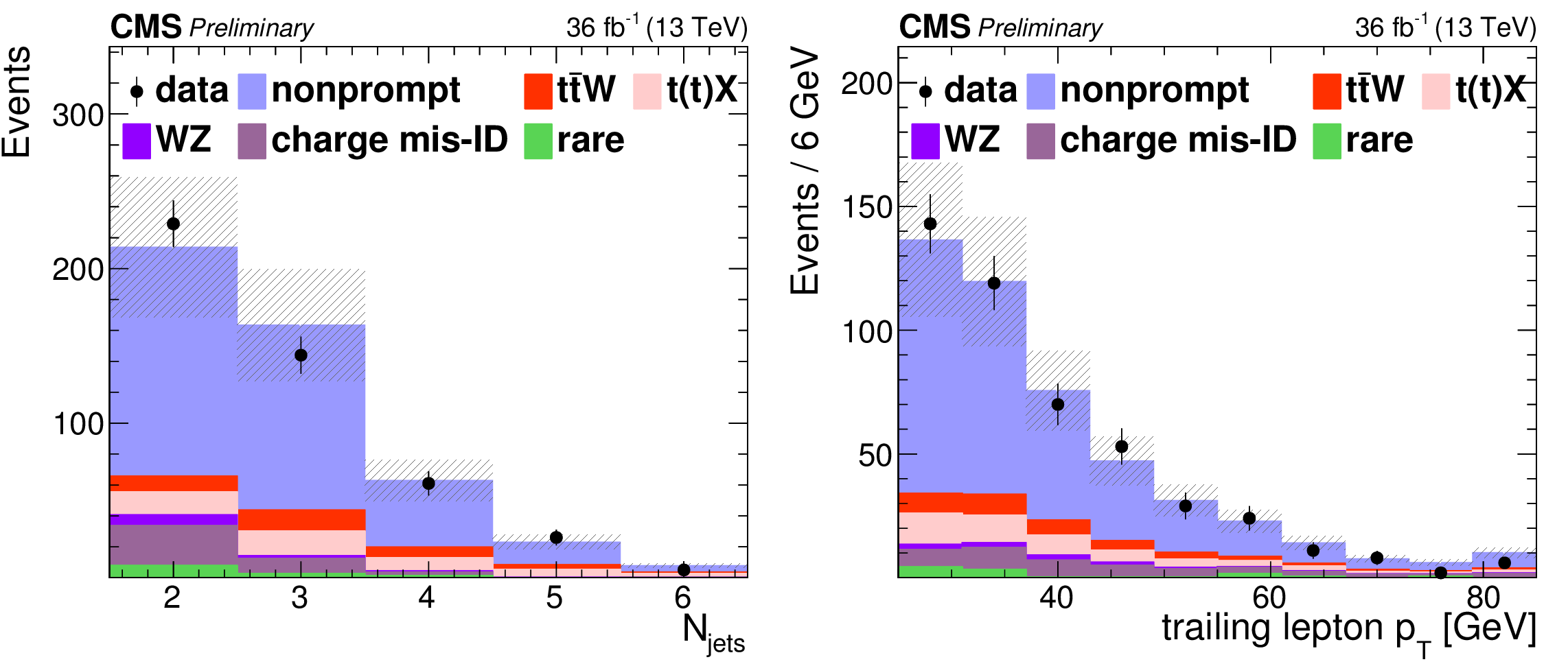
Figure 4:
Nonprompt control region plots in dilepton channel with BDT $<$ 0: distributions of the total yields versus jet multiplicity and transverse momentum of the trailing lepton. |

png pdf |
Figure 4-a:
Nonprompt control region plot in dilepton channel with BDT $<$ 0: distribution of the total yields versus jet multiplicity. |

png pdf |
Figure 4-b:
Nonprompt control region plot in dilepton channel with BDT $<$ 0: distribution of the total yields versus transverse momentum of the trailing lepton. |
png pdf |
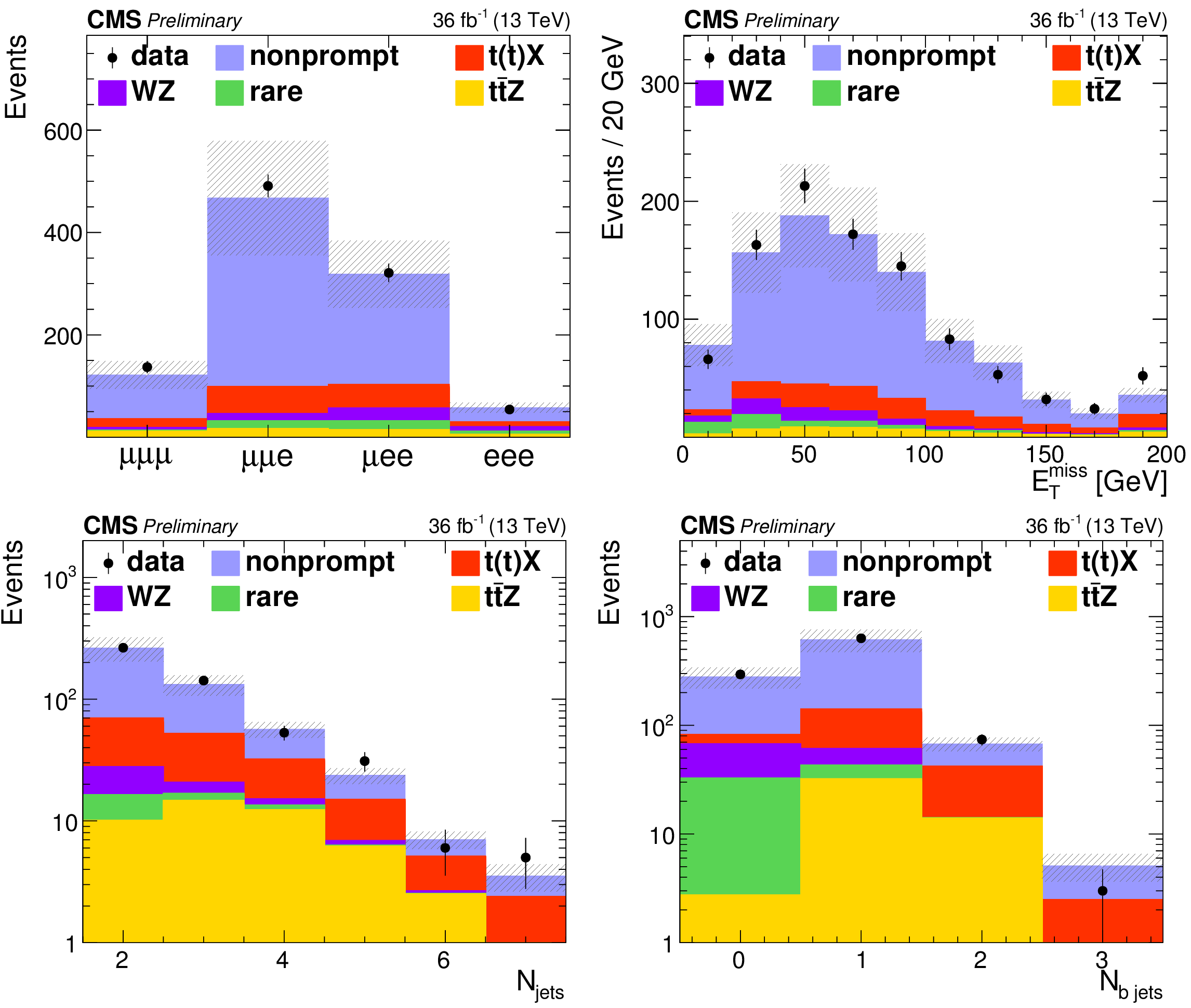
Figure 5:
Nonprompt control region plots in trilepton channel: distributions of the total yields versus lepton channel, missing transverse energy and (b-tagged) jet multiplicity. |

png pdf |
Figure 5-a:
Nonprompt control region plot in trilepton channel: distribution of the total yields versus lepton channel. |

png pdf |
Figure 5-b:
Nonprompt control region plot in trilepton channel: distribution of the total yields versus missing transverse energy. |
png pdf |
Figure 5-c:
Nonprompt control region plot in trilepton channel: distribution of the total yields versus b-tagged jet multiplicity. |

png pdf |
Figure 5-d:
Nonprompt control region plot in trilepton channel: distribution of the total yields versus jet multiplicity. |

png pdf |
Figure 6:
WZ control region plots: Distributions of the total yields versus lepton channel, jet multiplicity, transverse mass of the lepton and the missing transverse energy and the reconstructed invariant mass of the Z boson candidates. For all the plots the requirement on jet multiplicity is suppressed. |
png pdf |
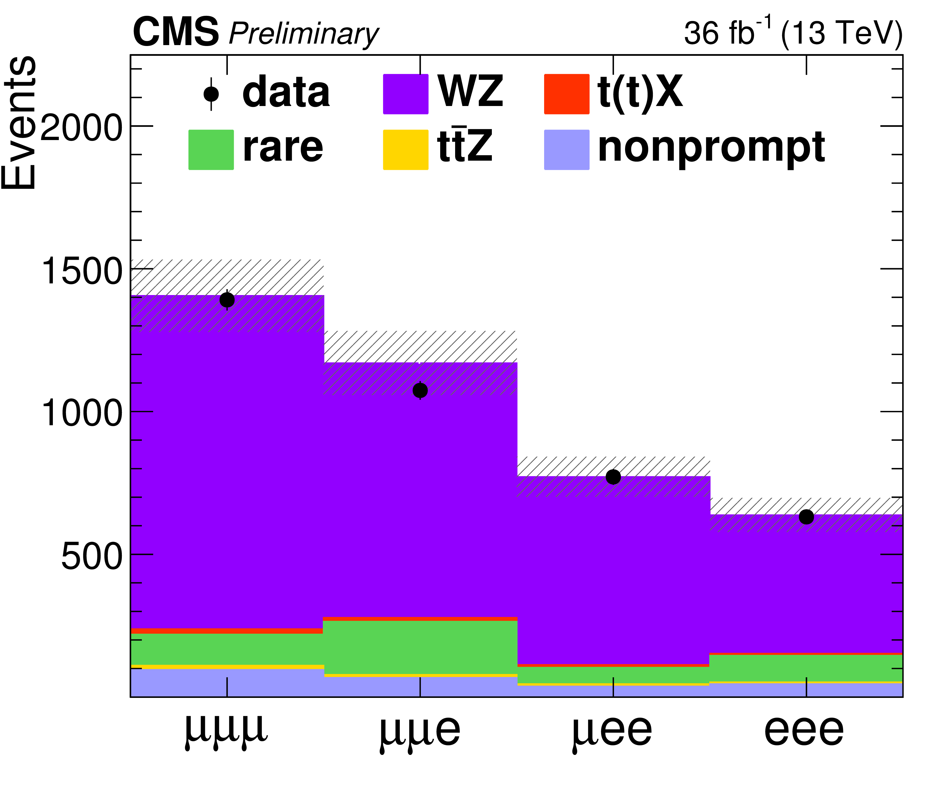
Figure 6-a:
WZ control region plot: Distribution of the total yields versus lepton channel. The requirement on jet multiplicity is suppressed. |
png pdf |
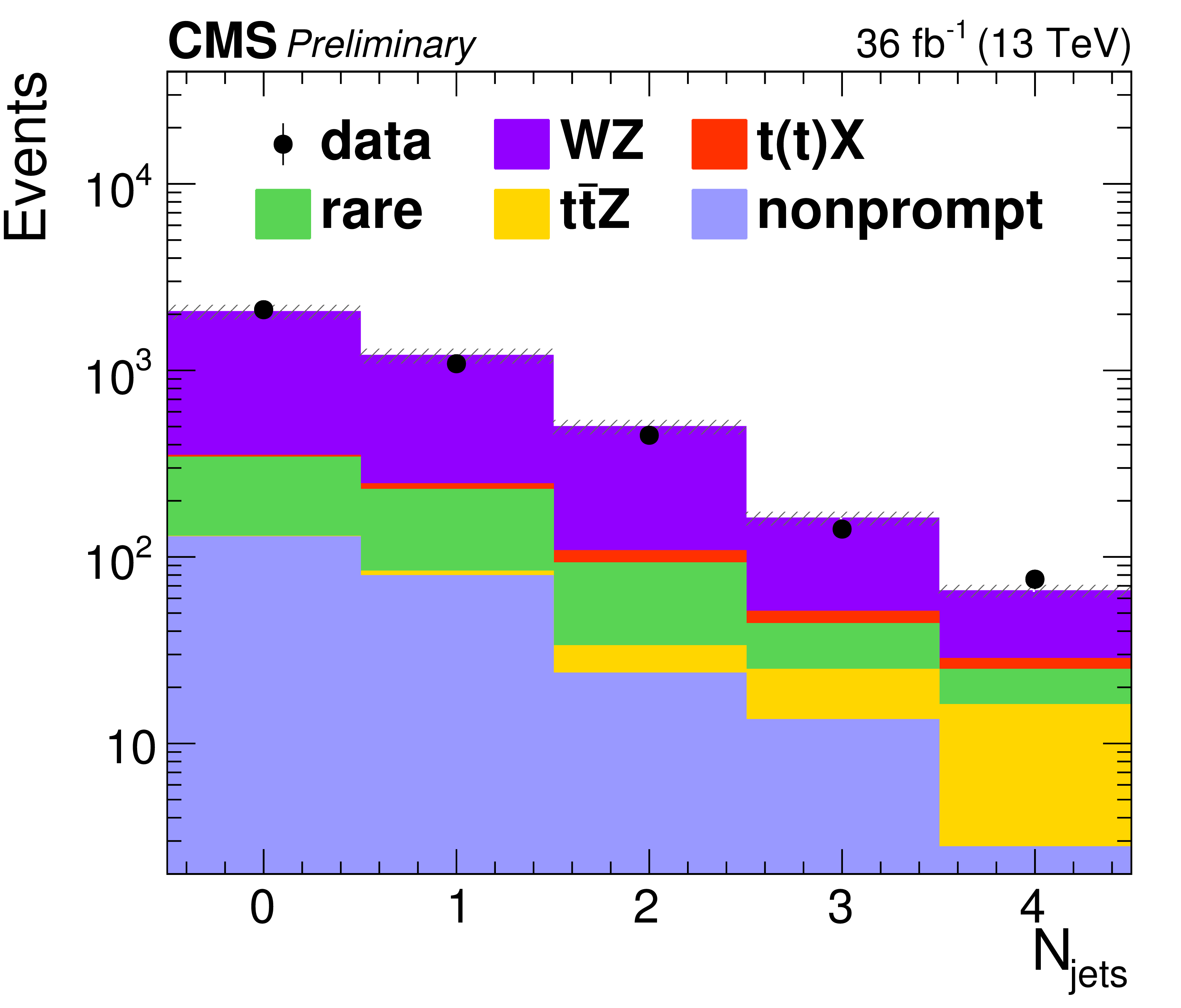
Figure 6-b:
WZ control region plot: Distribution of the total yields versus jet multiplicity. The requirement on jet multiplicity is suppressed. |
png pdf |
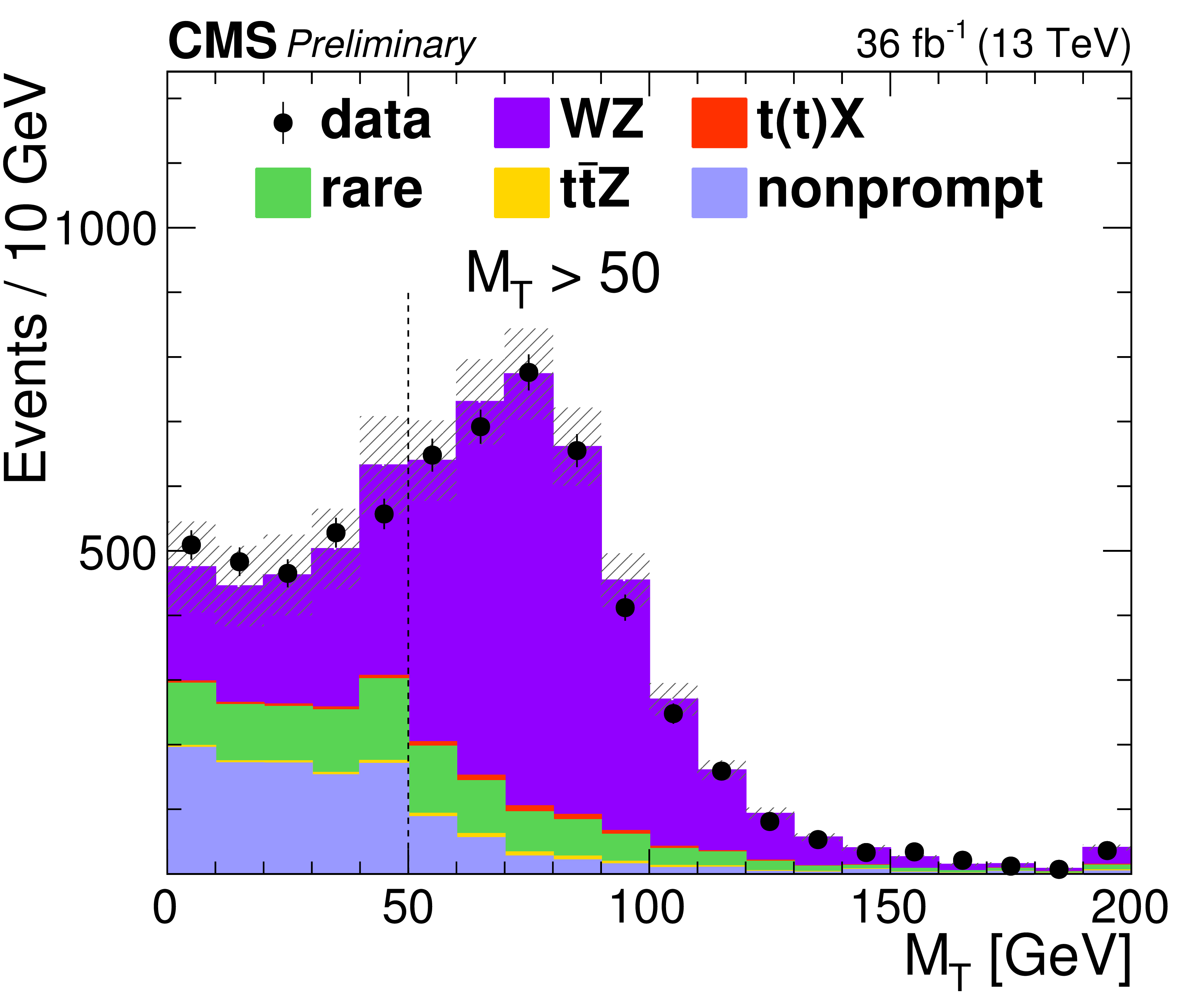
Figure 6-c:
WZ control region plot: Distribution of the total yields versus the transverse mass of the lepton and the missing transverse energy. The requirement on jet multiplicity is suppressed. |
png pdf |
Figure 6-d:
WZ control region plot: Distribution of the total yields versus the reconstructed invariant mass of the Z boson candidates. The requirement on jet multiplicity is suppressed. |
png pdf |
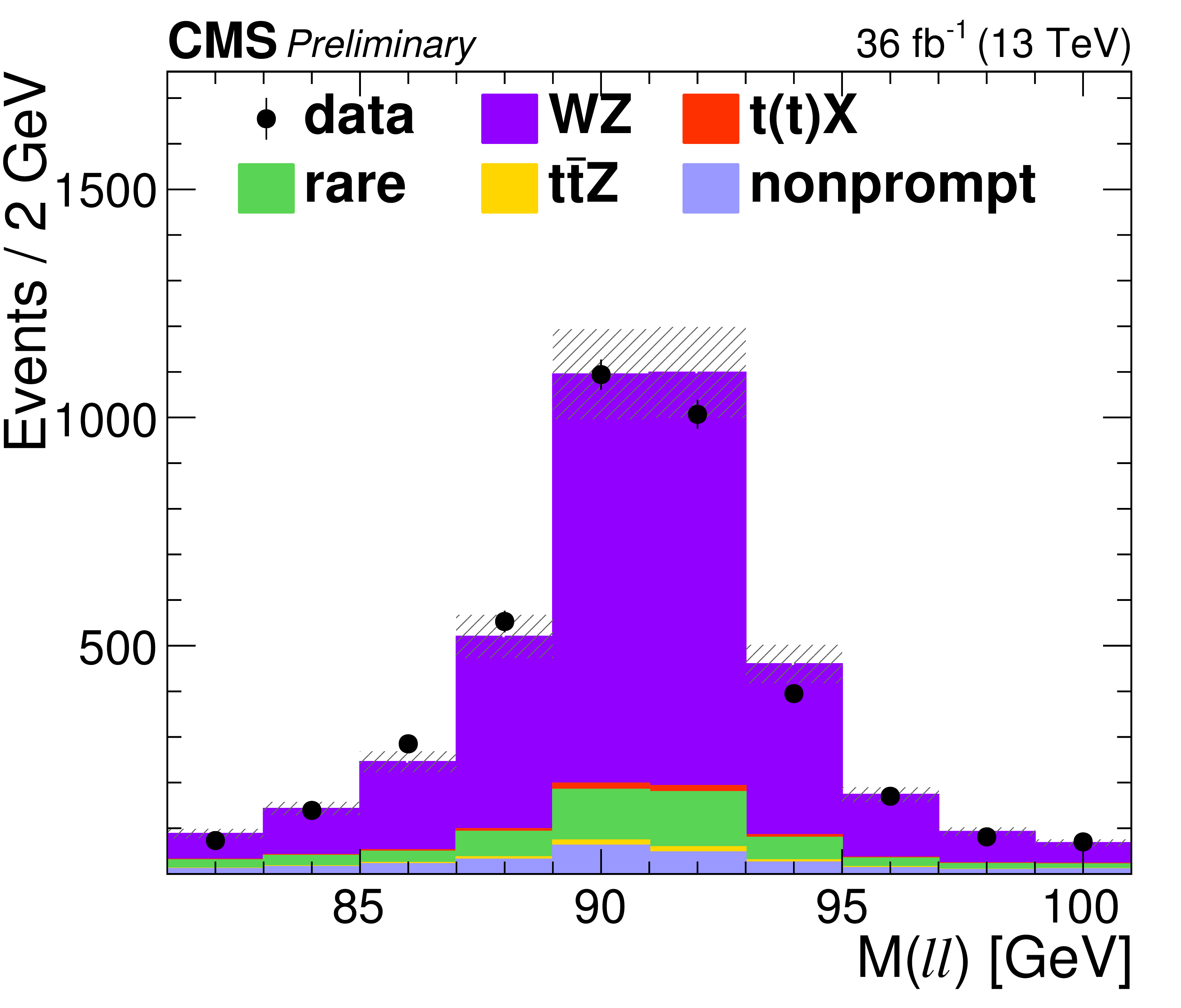
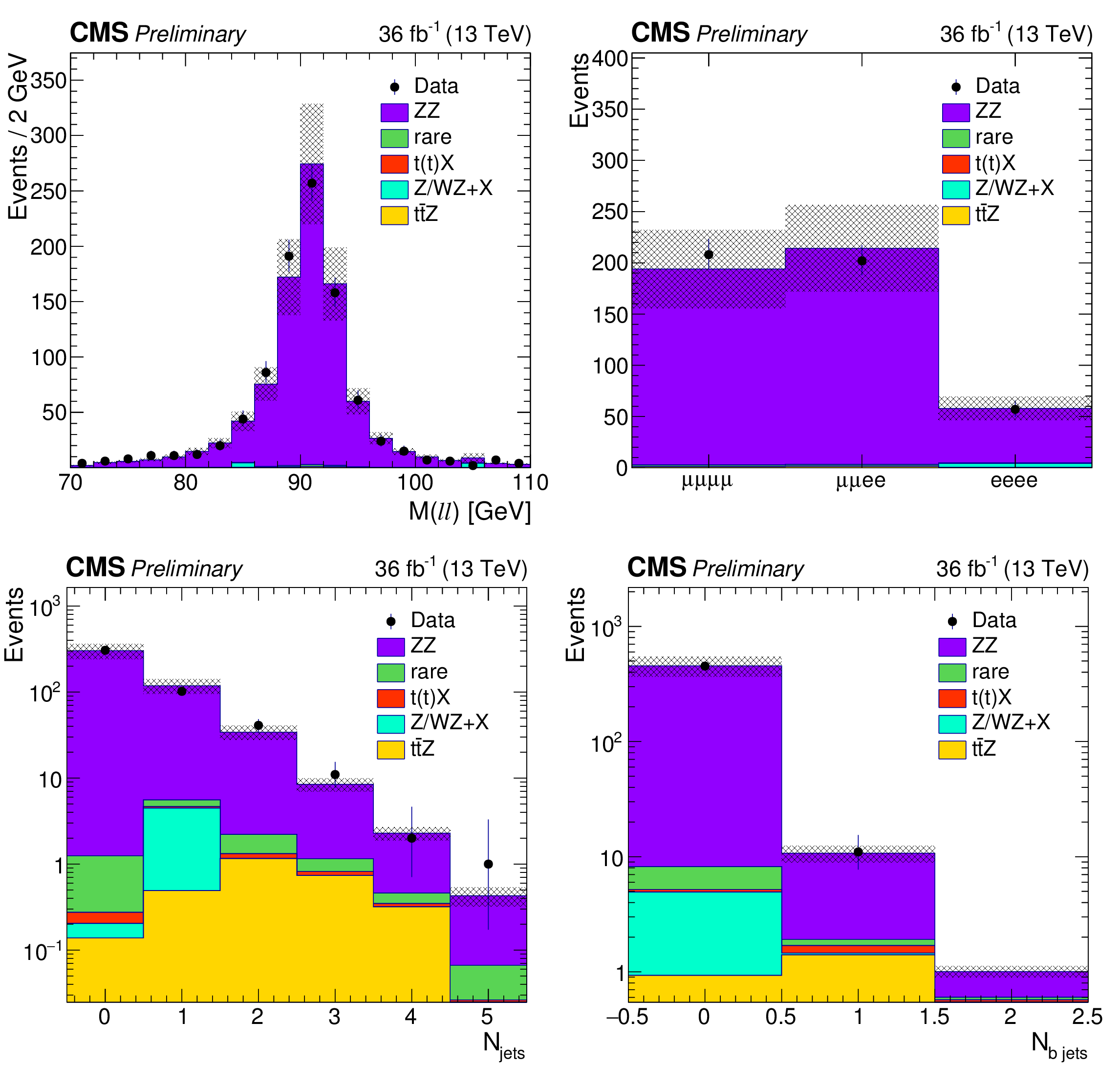
Figure 7:
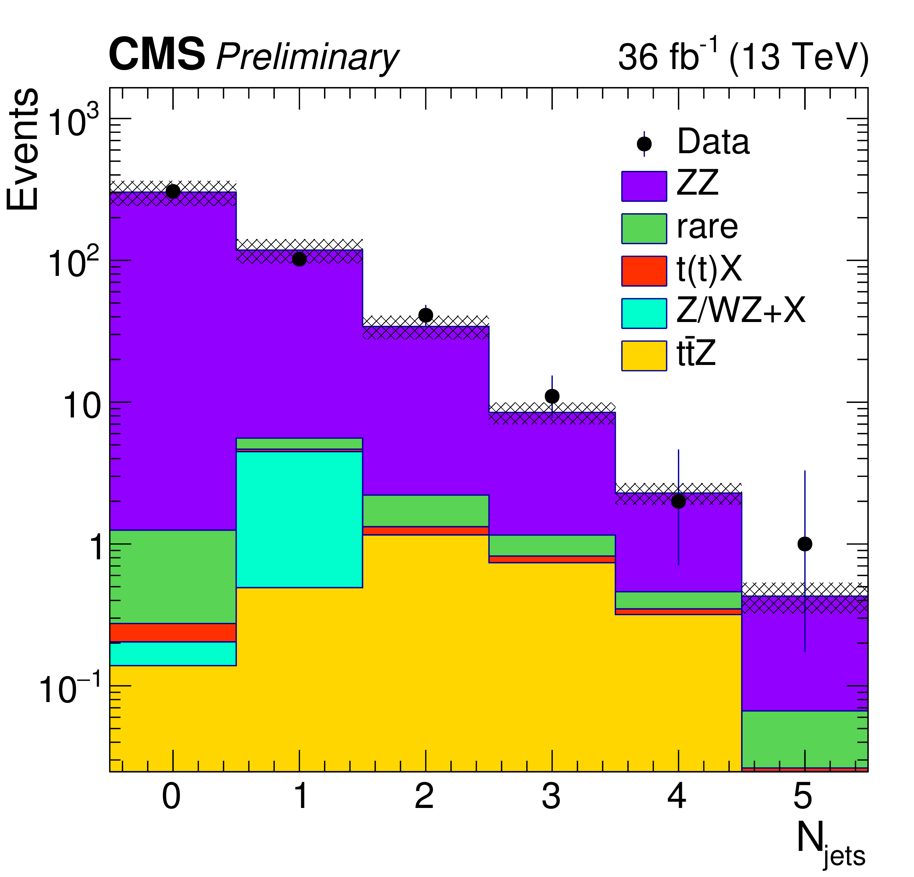
Data-MC comparison for the Z candidates mass (top left), event yields (top right), jet multiplicity (bottom left) and b-jet multiplicity (bottom right) in a ZZ-dominated background control region |
png pdf |
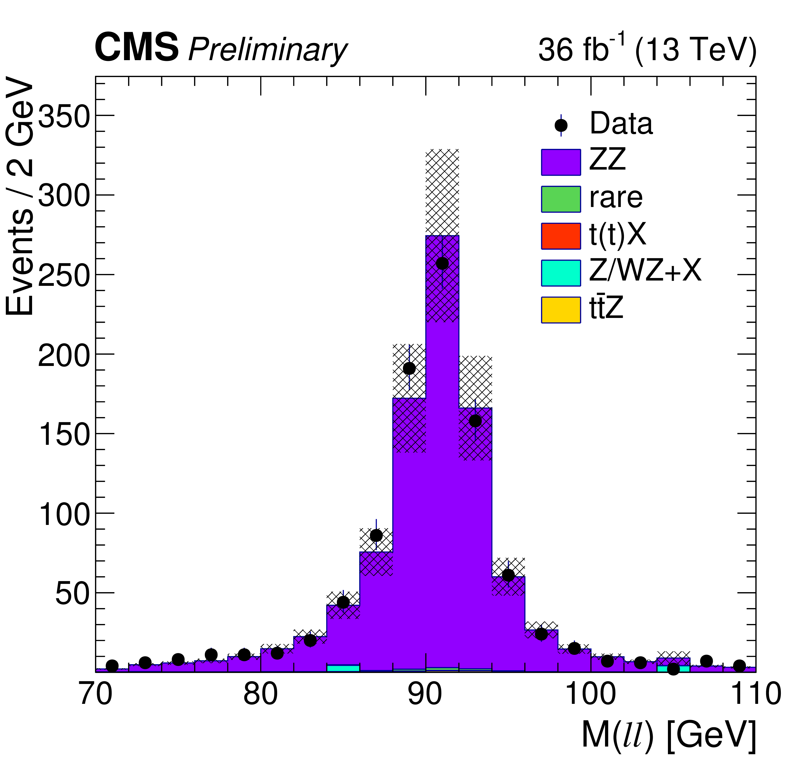
Figure 7-a:
Data-MC comparison for the Z candidates mass in a ZZ-dominated background control region |
png pdf |
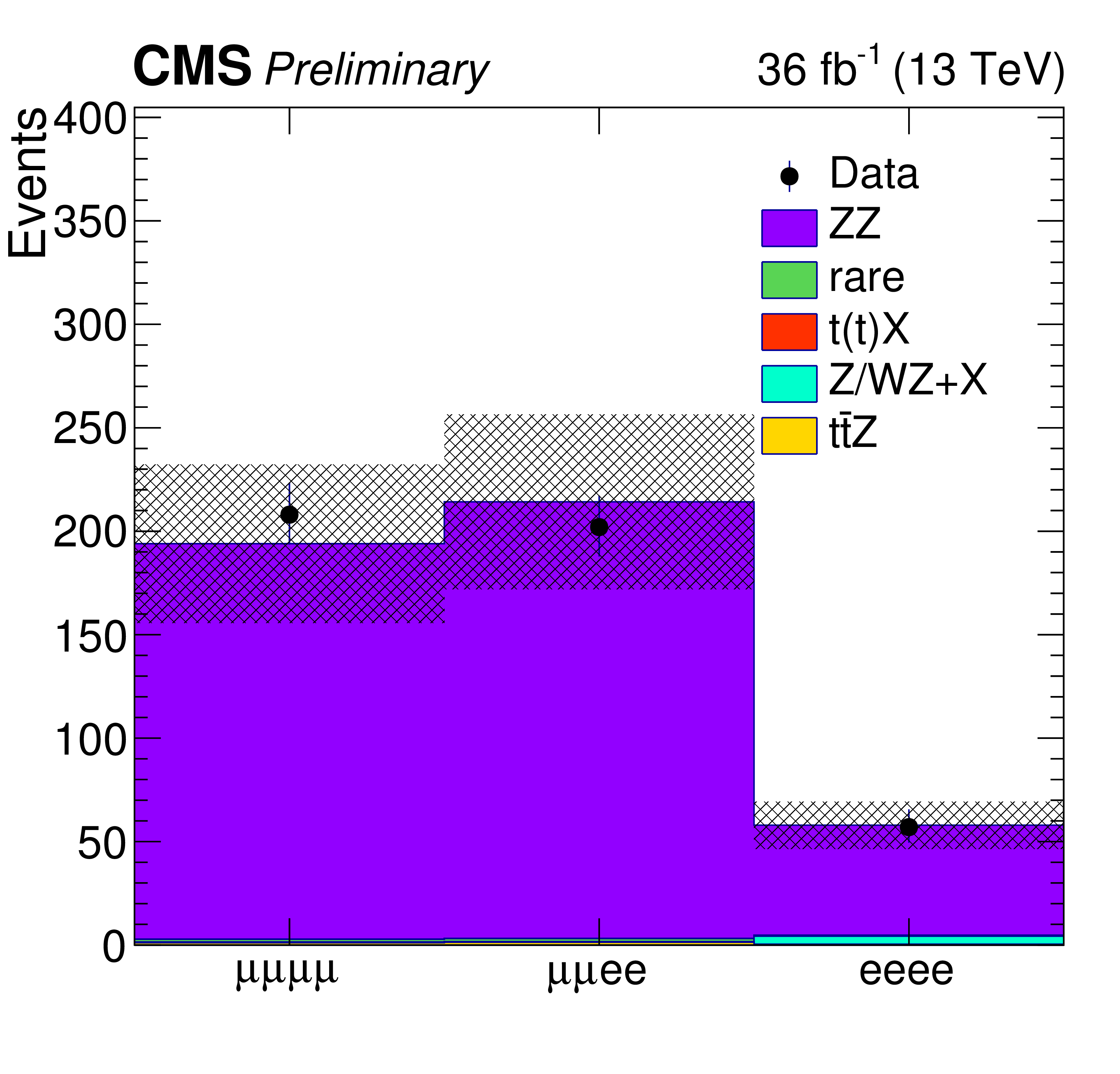
Figure 7-b:
Data-MC comparison for the event yields in a ZZ-dominated background control region |
png pdf |
Figure 7-c:
Data-MC comparison for the jet multiplicity in a ZZ-dominated background control region |

png pdf |
Figure 7-d:
Data-MC comparison for the b-jet multiplicity in a ZZ-dominated background control region |
png pdf |
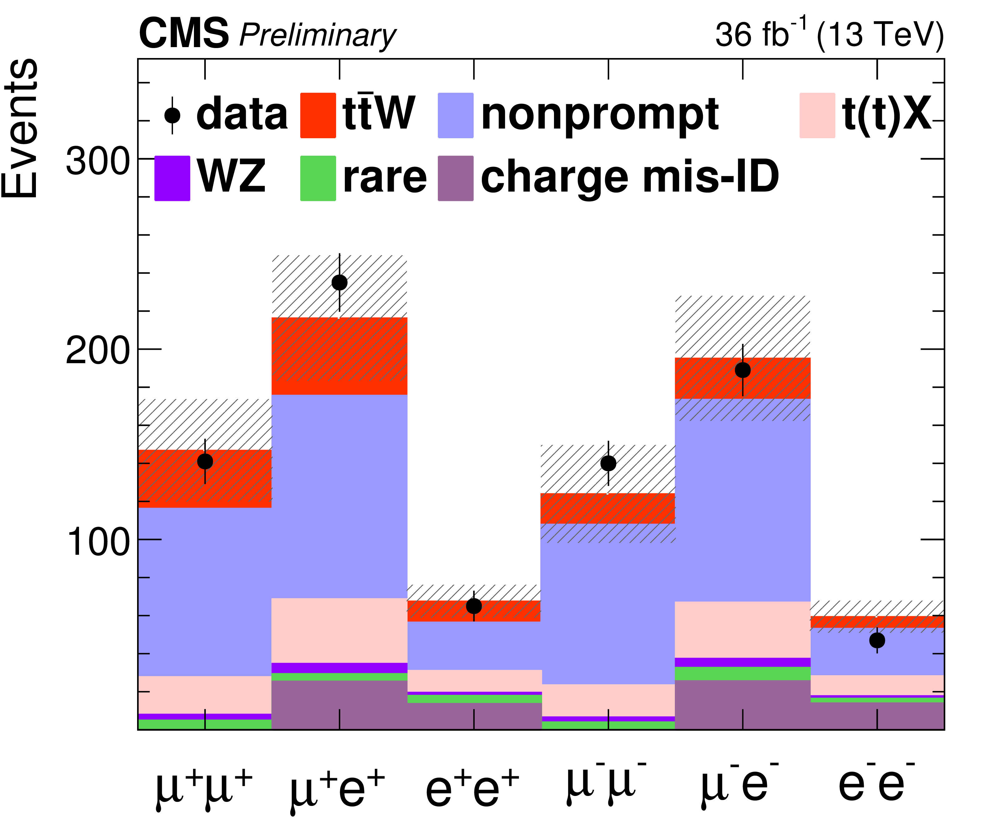
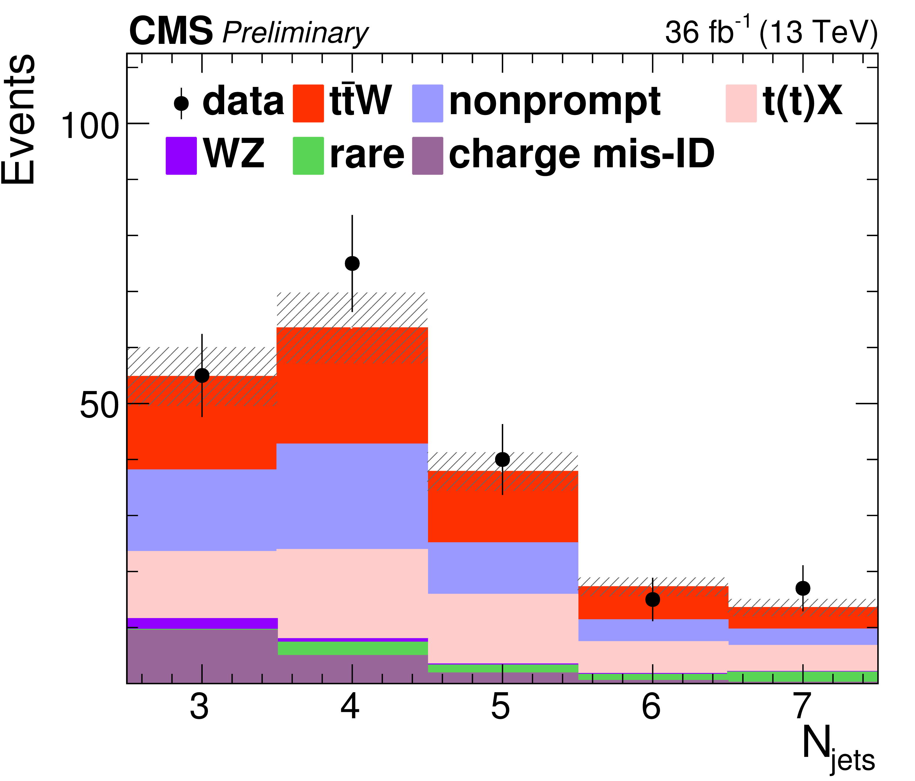
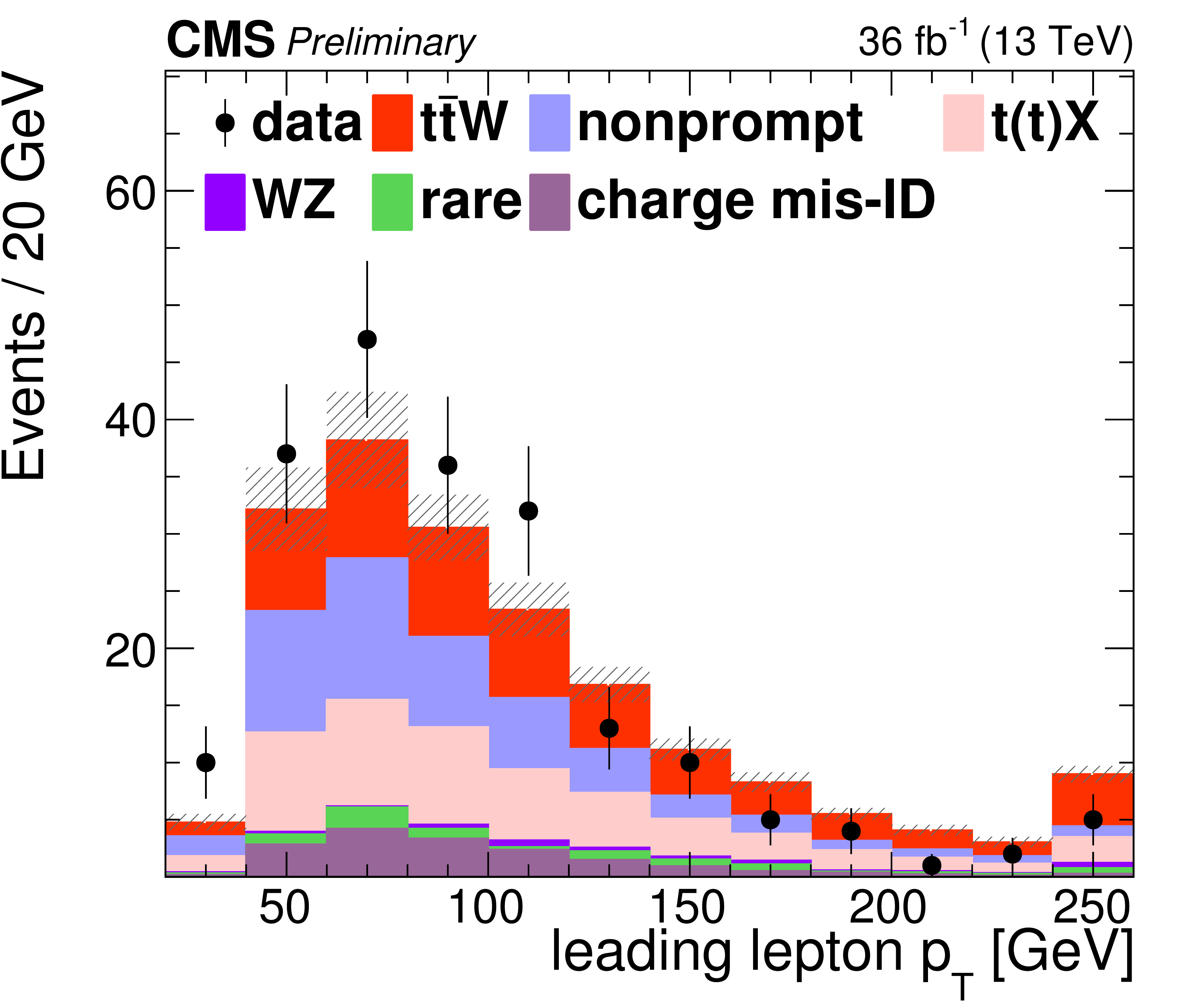
Figure 8:
Distributions of the predicted and observed yields versus the kinematic variables in ${{\mathrm{ t } {}\mathrm{ \bar{t} } } \mathrm{ W } } $ signal enriched region for same charge dilepton channel. |
png pdf |
Figure 8-a:
Distribution of the predicted and observed yields in ${{\mathrm{ t } {}\mathrm{ \bar{t} } } \mathrm{ W } } $ signal enriched region for same charge dilepton channel. |
png pdf |
Figure 8-b:
Distribution of the predicted and observed yields in ${{\mathrm{ t } {}\mathrm{ \bar{t} } } \mathrm{ W } } $ signal enriched region for same charge dilepton channel. |
png pdf |
Figure 8-c:
Distribution of the predicted and observed yields in ${{\mathrm{ t } {}\mathrm{ \bar{t} } } \mathrm{ W } } $ signal enriched region for same charge dilepton channel. |
png pdf |
Figure 8-d:
Distribution of the predicted and observed yields in ${{\mathrm{ t } {}\mathrm{ \bar{t} } } \mathrm{ W } } $ signal enriched region for same charge dilepton channel. |
png pdf |
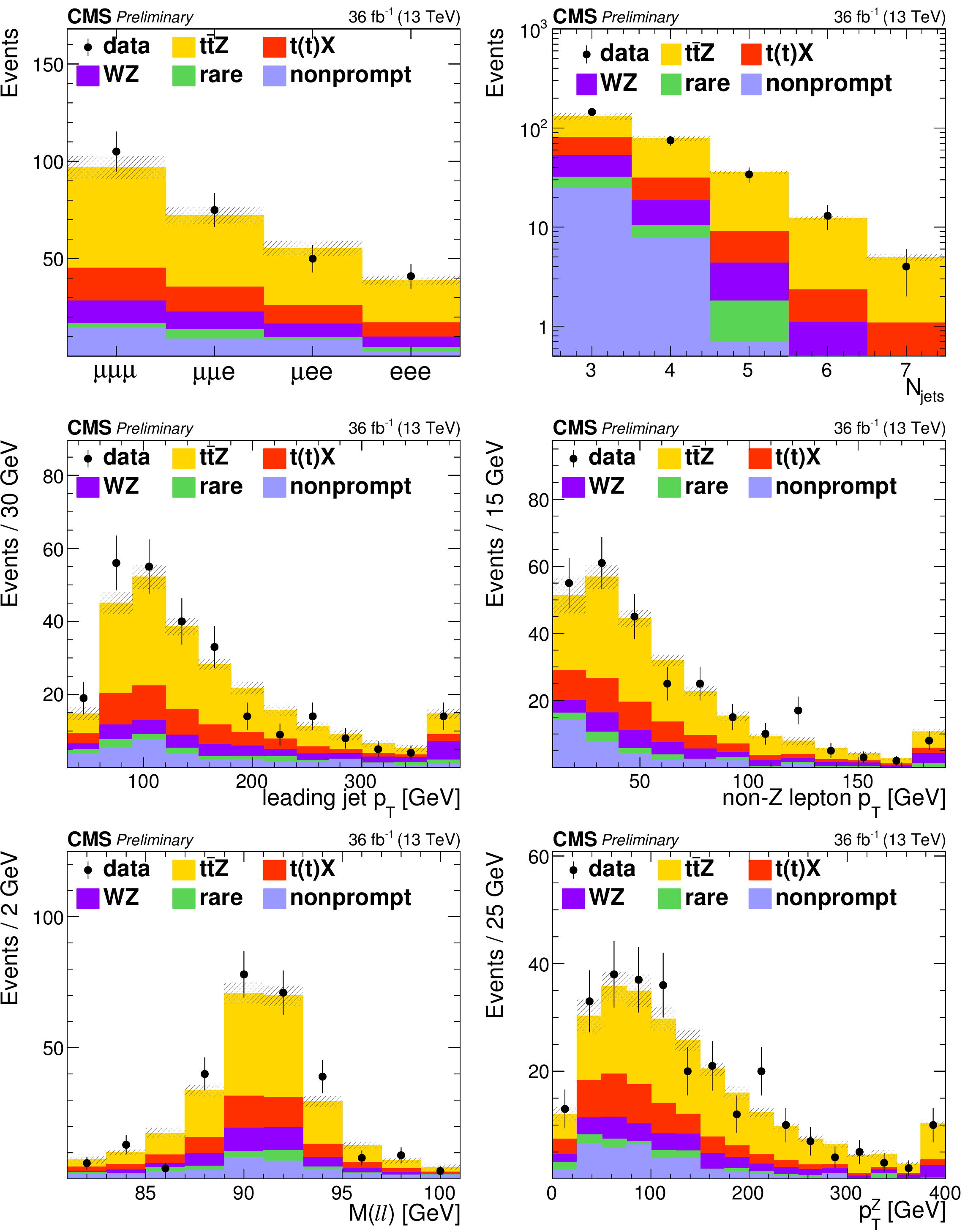
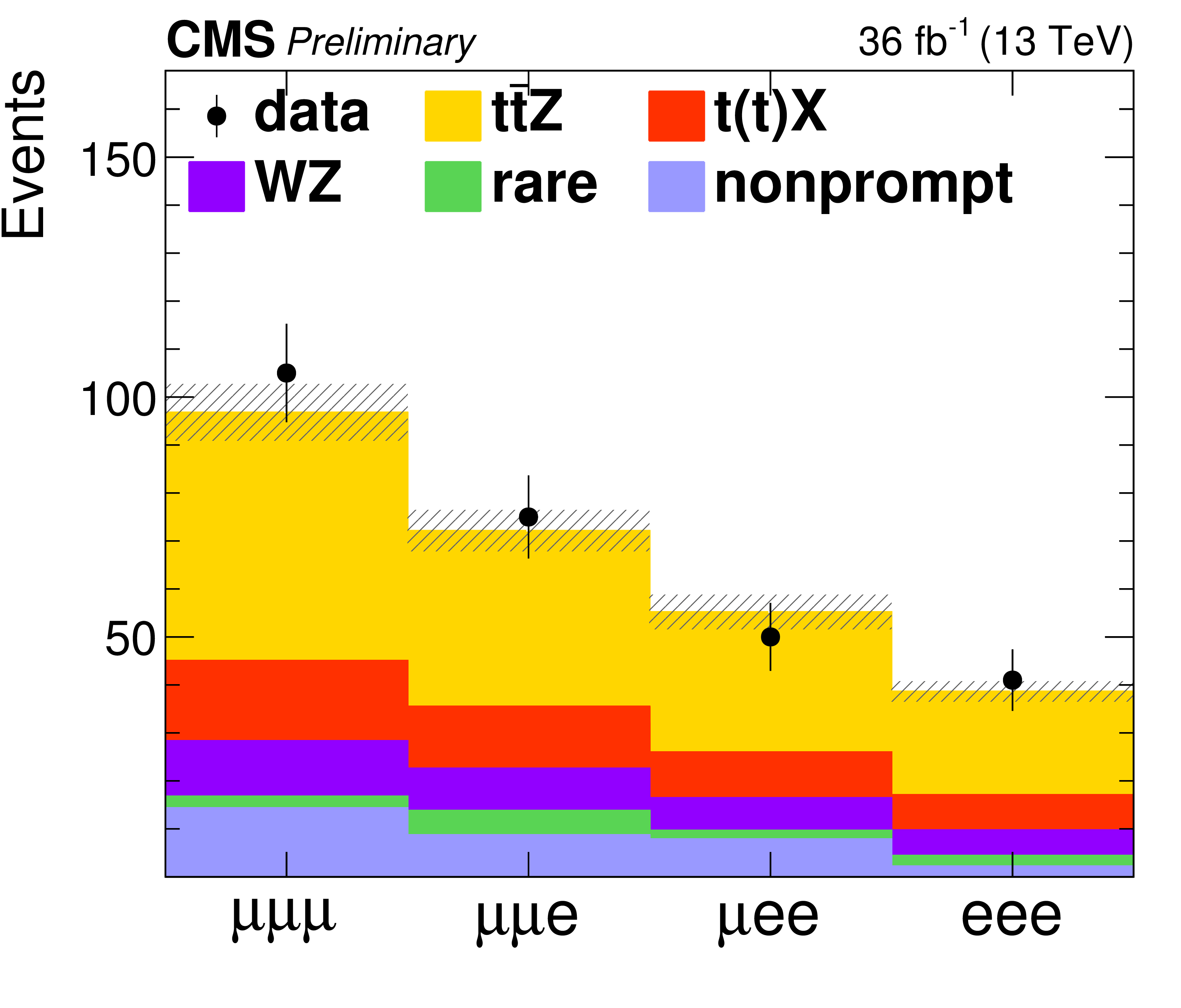
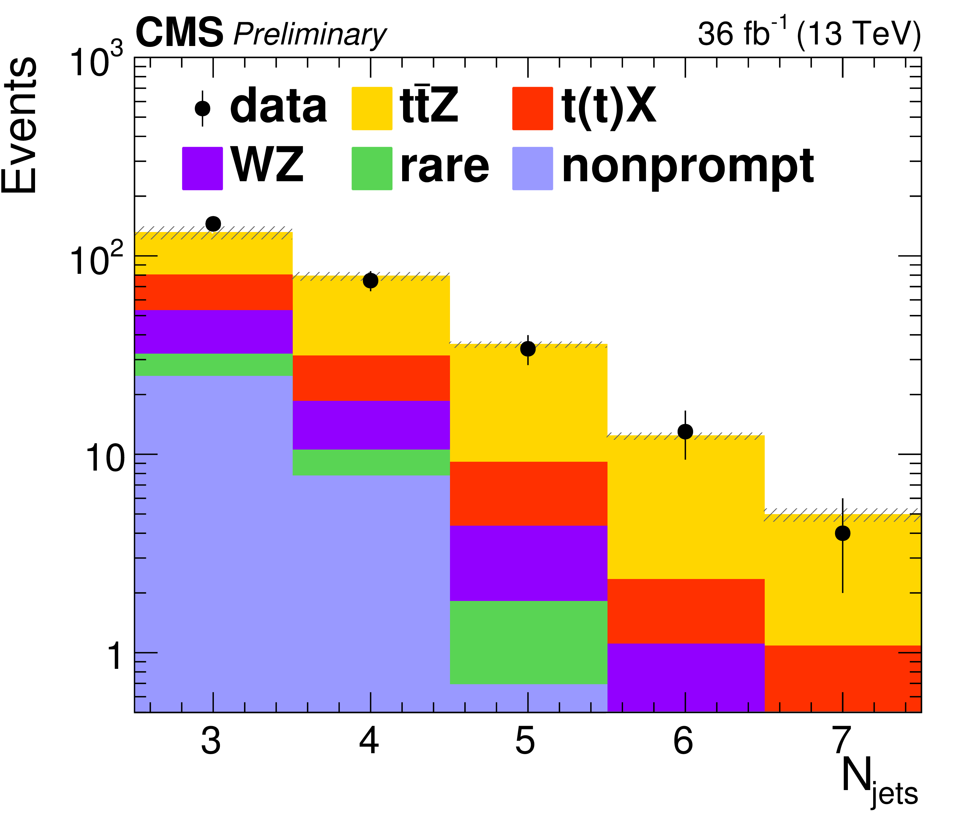
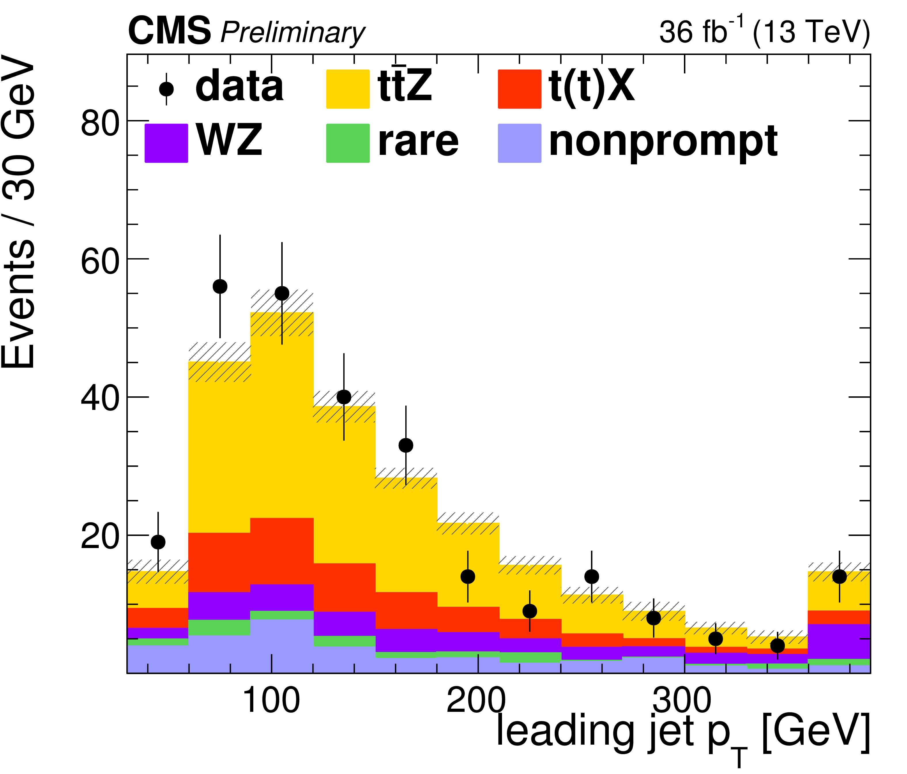
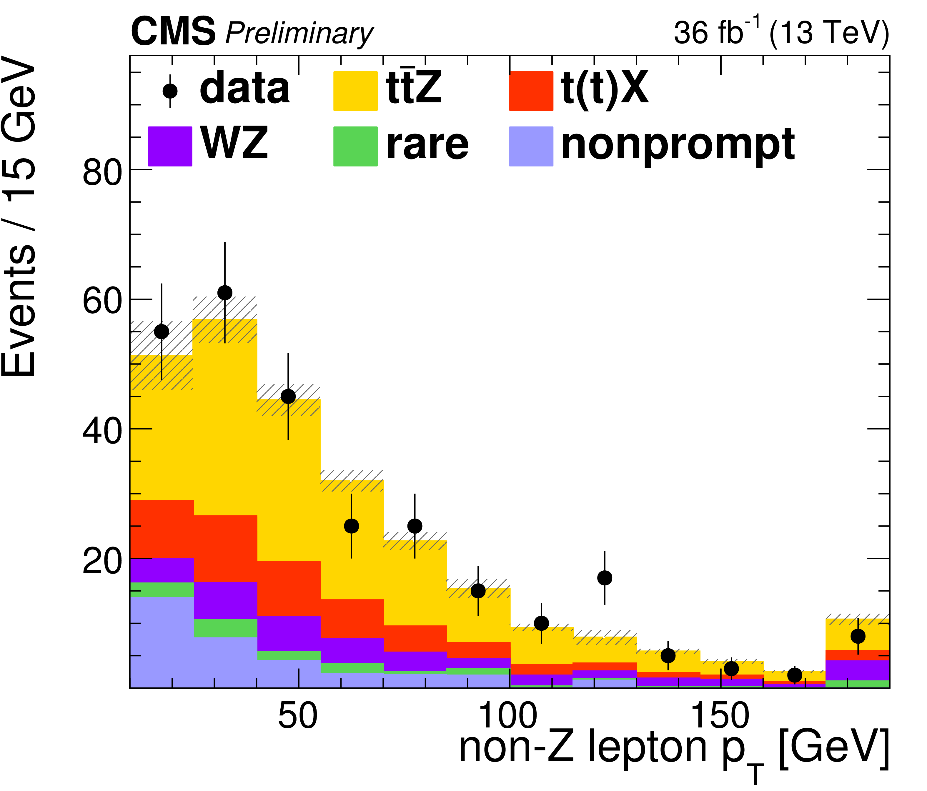
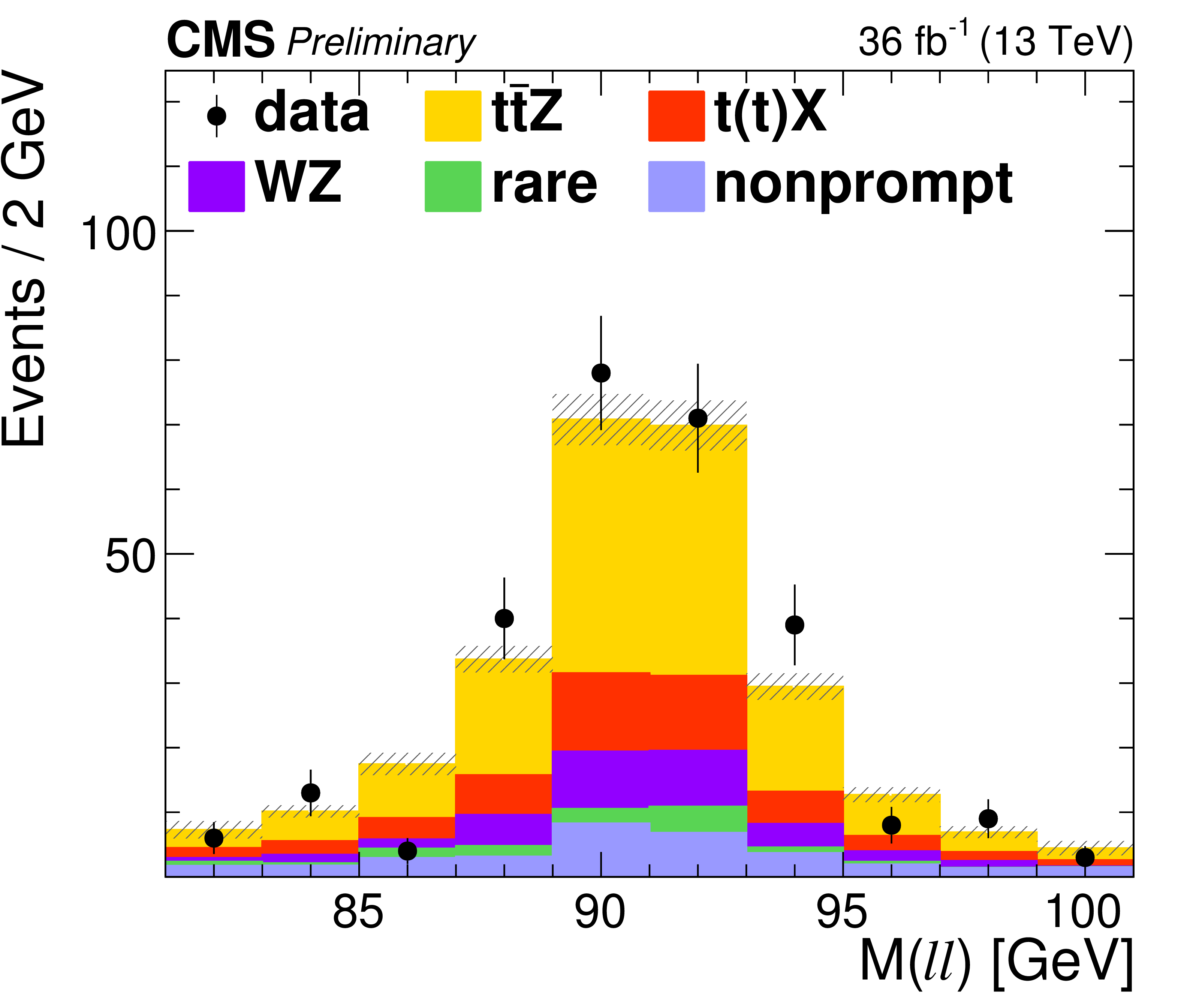
Figure 9:
Distributions of the predicted and observed yields versus the kinematic variables in ${{\mathrm{ t } {}\mathrm{ \bar{t} } } \mathrm{ Z } } $ signal enriched region for three lepton channel. |
png pdf |
Figure 9-a:
Distribution of the predicted and observed yields in ${{\mathrm{ t } {}\mathrm{ \bar{t} } } \mathrm{ Z } } $ signal enriched region for three lepton channel. |
png pdf |
Figure 9-b:
Distribution of the predicted and observed yields in ${{\mathrm{ t } {}\mathrm{ \bar{t} } } \mathrm{ Z } } $ signal enriched region for three lepton channel. |
png pdf |
Figure 9-c:
Distribution of the predicted and observed yields in ${{\mathrm{ t } {}\mathrm{ \bar{t} } } \mathrm{ Z } } $ signal enriched region for three lepton channel. |
png pdf |
Figure 9-d:
Distribution of the predicted and observed yields in ${{\mathrm{ t } {}\mathrm{ \bar{t} } } \mathrm{ Z } } $ signal enriched region for three lepton channel. |
png pdf |
Figure 9-e:
Distribution of the predicted and observed yields in ${{\mathrm{ t } {}\mathrm{ \bar{t} } } \mathrm{ Z } } $ signal enriched region for three lepton channel. |
png pdf |
Figure 9-f:
Distribution of the predicted and observed yields in ${{\mathrm{ t } {}\mathrm{ \bar{t} } } \mathrm{ Z } } $ signal enriched region for three lepton channel. |
png pdf |
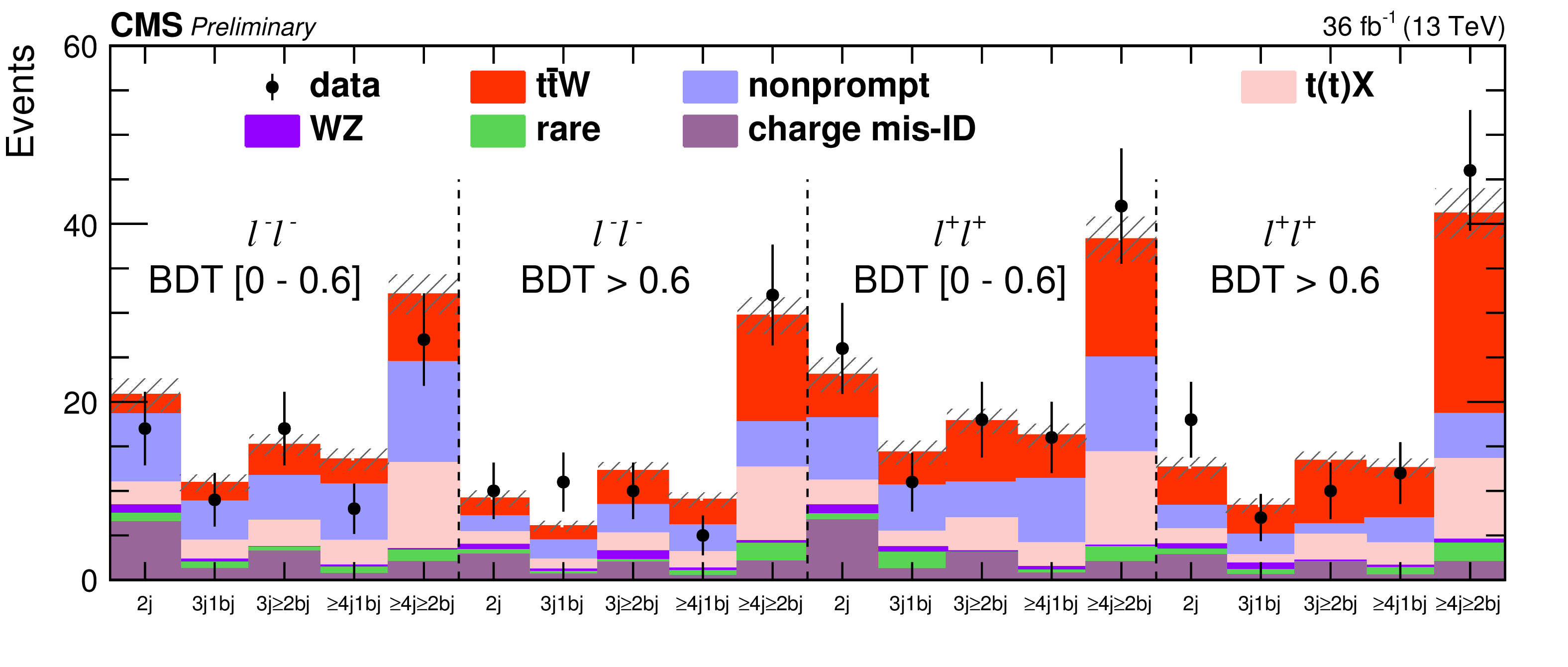
Figure 10:
Post-fit predicted and observed yields in each analysis bin in the same-sign dilepton analysis.The hatched band shows the total uncertainty associated to signal and background predictions. |
png pdf |
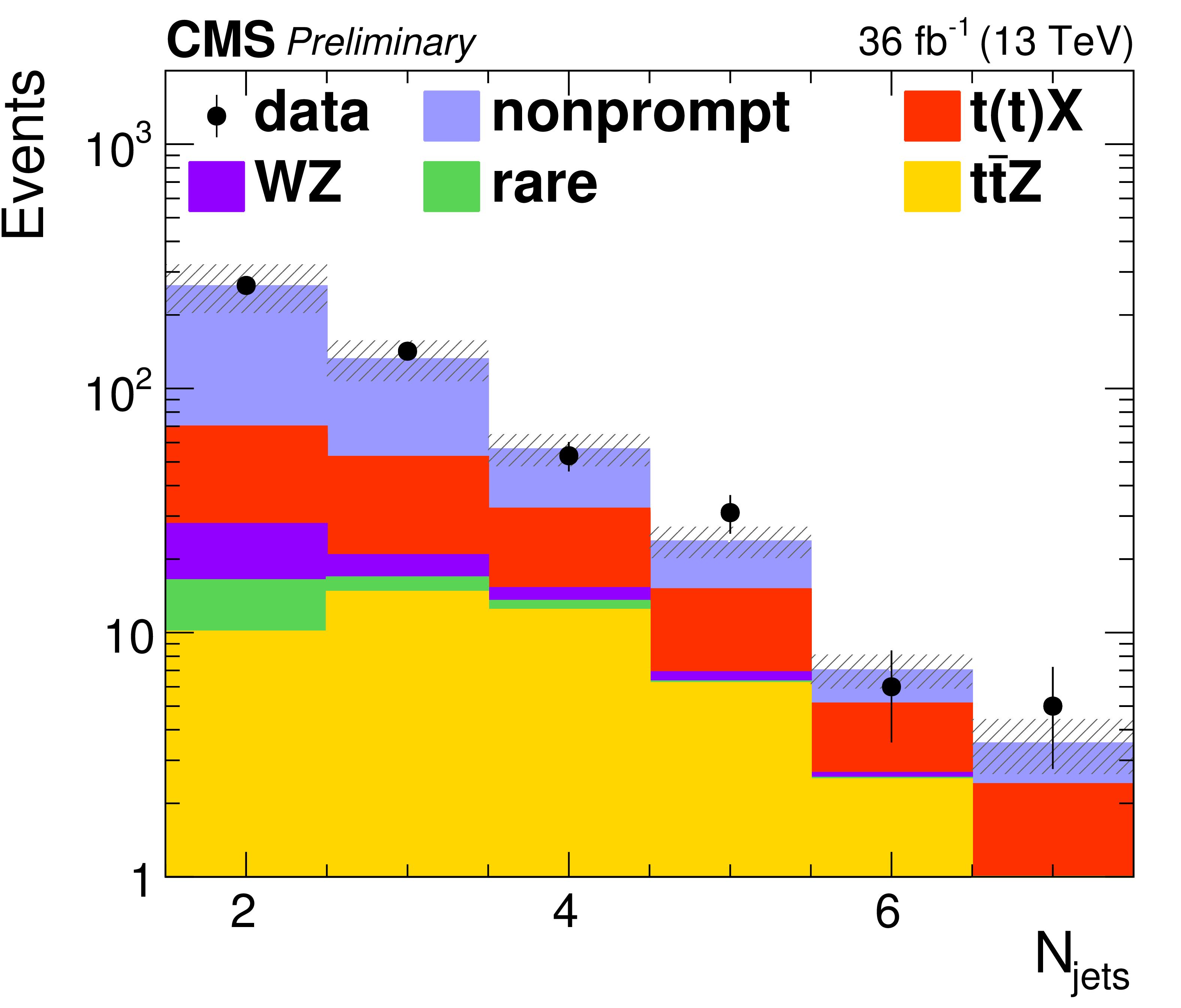
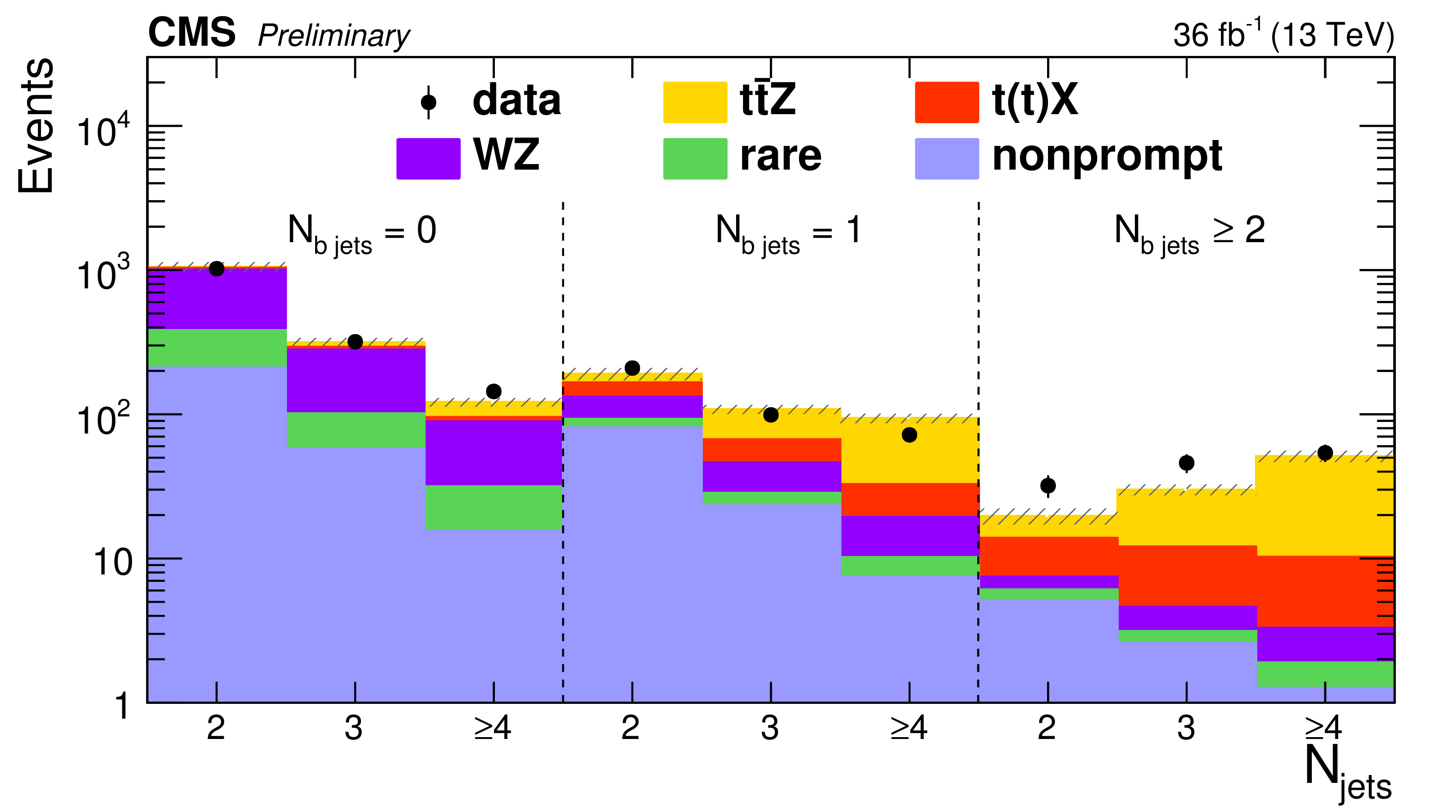
Figure 11:
Post-fit predicted and observed yields in $ {N_\text {jets}} = $ 2, 3 and $\geq $4 categories in the three-lepton analyses. The hatched band shows the total uncertainty associated to signal and background predictions. |
png pdf |
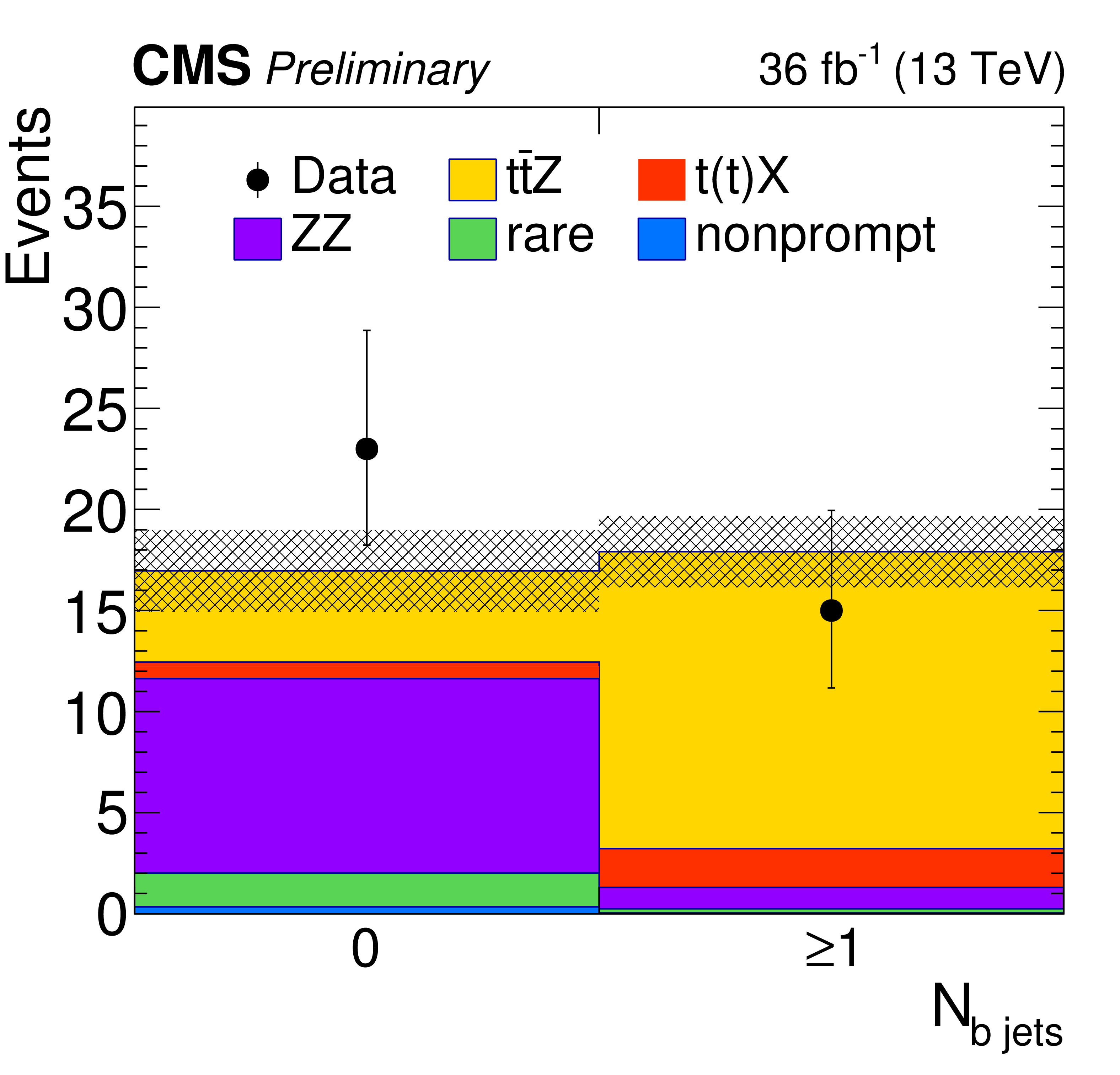
Figure 12:
Post-fit predicted and observed yields in the four-lepton analyses. The hatched band shows the total uncertainty associated to signal and background predictions. |
png pdf |
Figure 13:
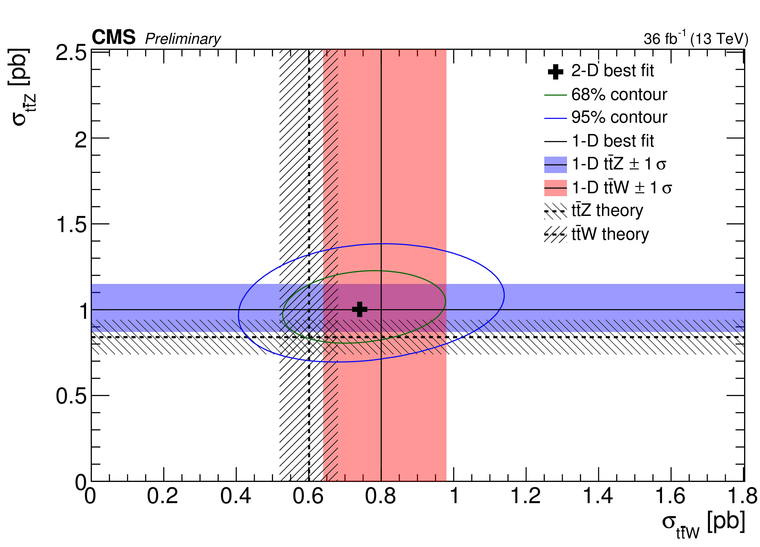
The result of the two-dimensional best fit for ${{\mathrm{ t } {}\mathrm{ \bar{t} } } \mathrm{ W } }$ and ${{\mathrm{ t } {}\mathrm{ \bar{t} } } \mathrm{ Z } }$ cross sections (cross symbol) is shown along with its 68 and 95% confidence level contours. The result of this fit is superimposed with the separate ${{\mathrm{ t } {}\mathrm{ \bar{t} } } \mathrm{ W } }$ and ${{\mathrm{ t } {}\mathrm{ \bar{t} } } \mathrm{ Z } }$ cross section measurements, and the corresponding 1$\sigma $ bands, obtained from the dilepton, and the three-lepton/four-lepton channels, respectively. The figure also shows the predictions from theory and the corresponding uncertainties. |
png pdf |
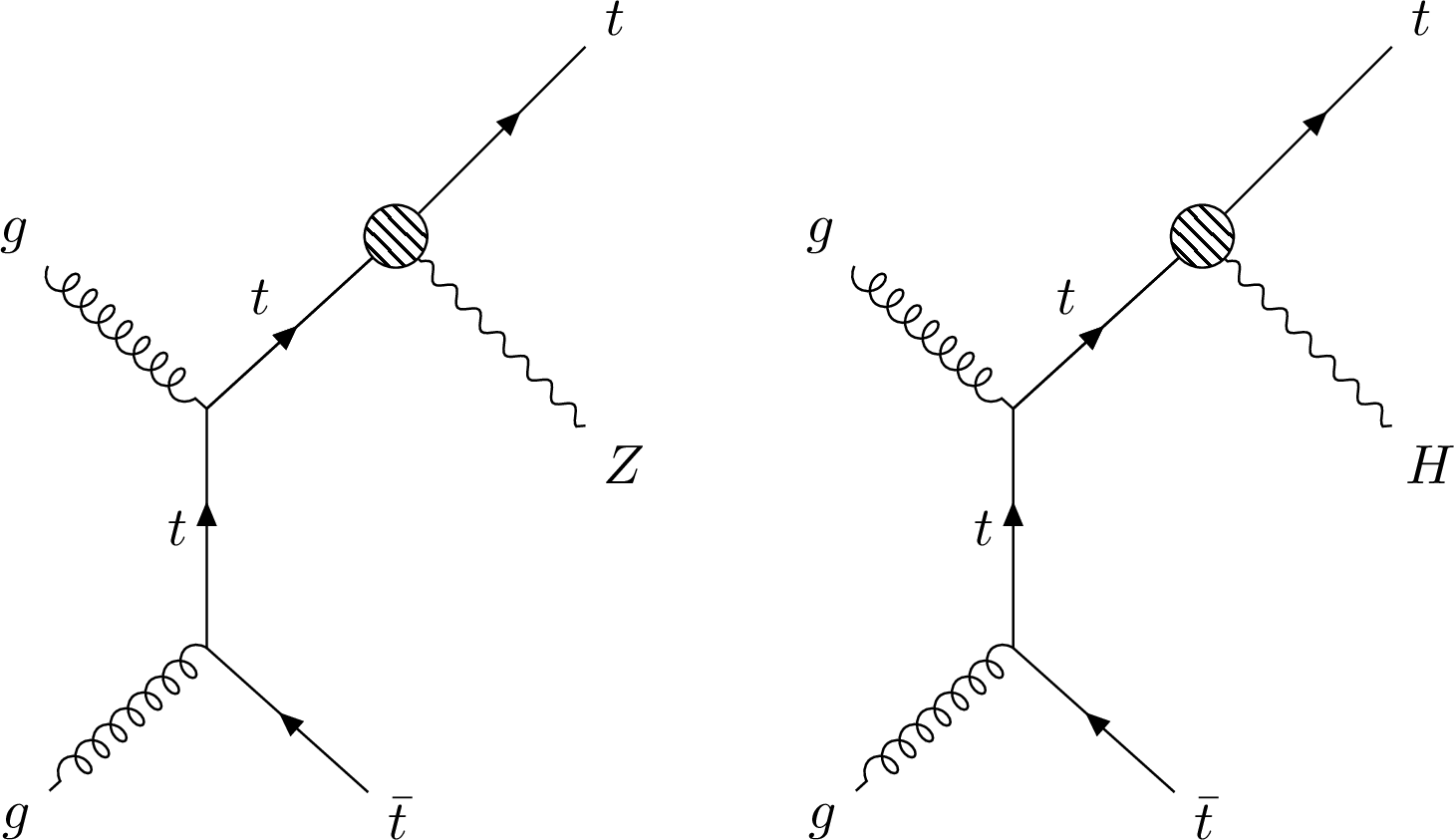
Figure 14:
Leading order Feynman diagrams involving NP vertices due to the operator which is proportional to $ {\bar{c}_{uB}} $, $ {\bar{c}_{uW}} $, and $ {\bar{c}_{Hu}} $ (left), and $ {\bar{c}_{u}} $ (right). |

png pdf |
Figure 14-a:
Leading order Feynman diagram involving the NP vertex due to the operator which is proportional to $ {\bar{c}_{uB}} $, $ {\bar{c}_{uW}} $, and $ {\bar{c}_{Hu}} $. |
png pdf |
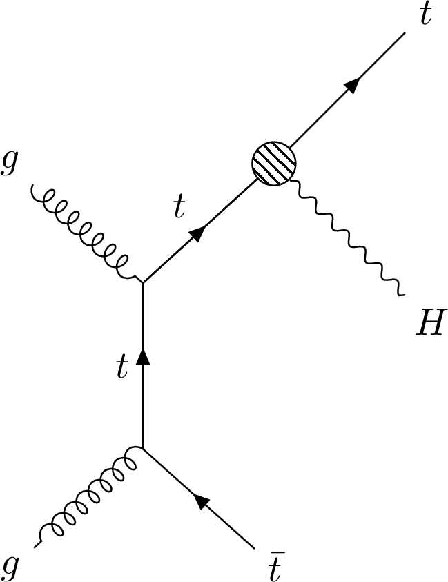
Figure 14-b:
Leading order Feynman diagram involving the NP vertex due to the operator which is proportional to $ {\bar{c}_{u}} $. |
png pdf |
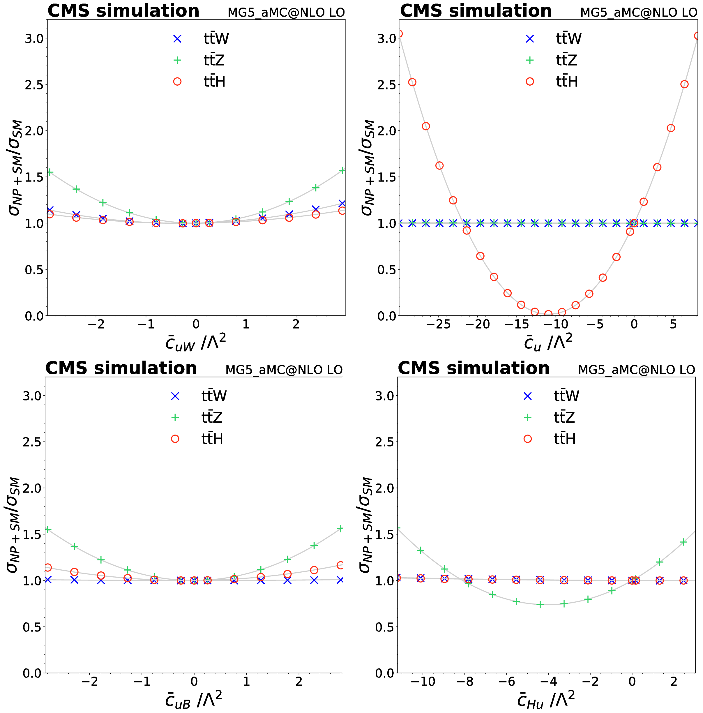
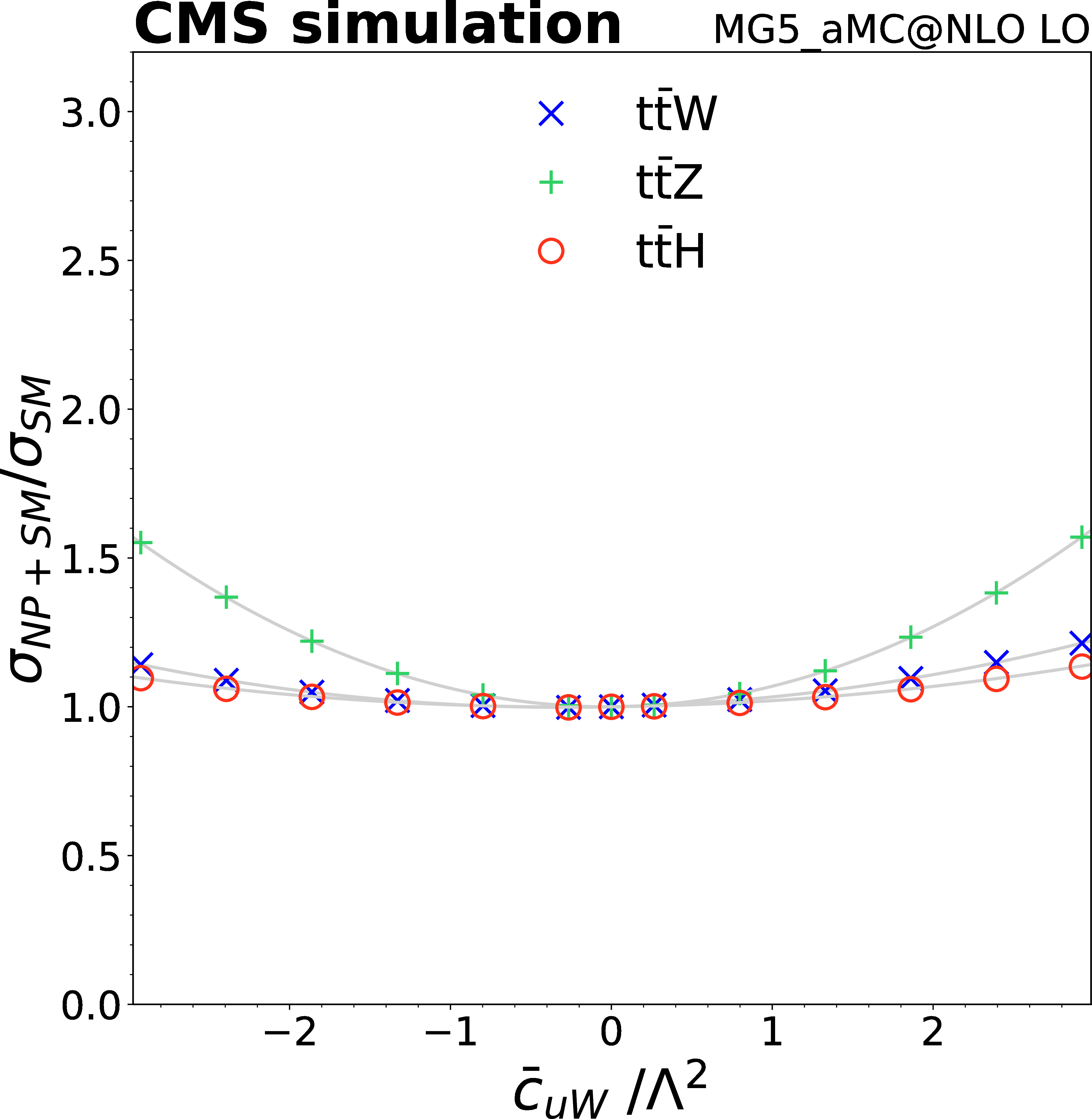
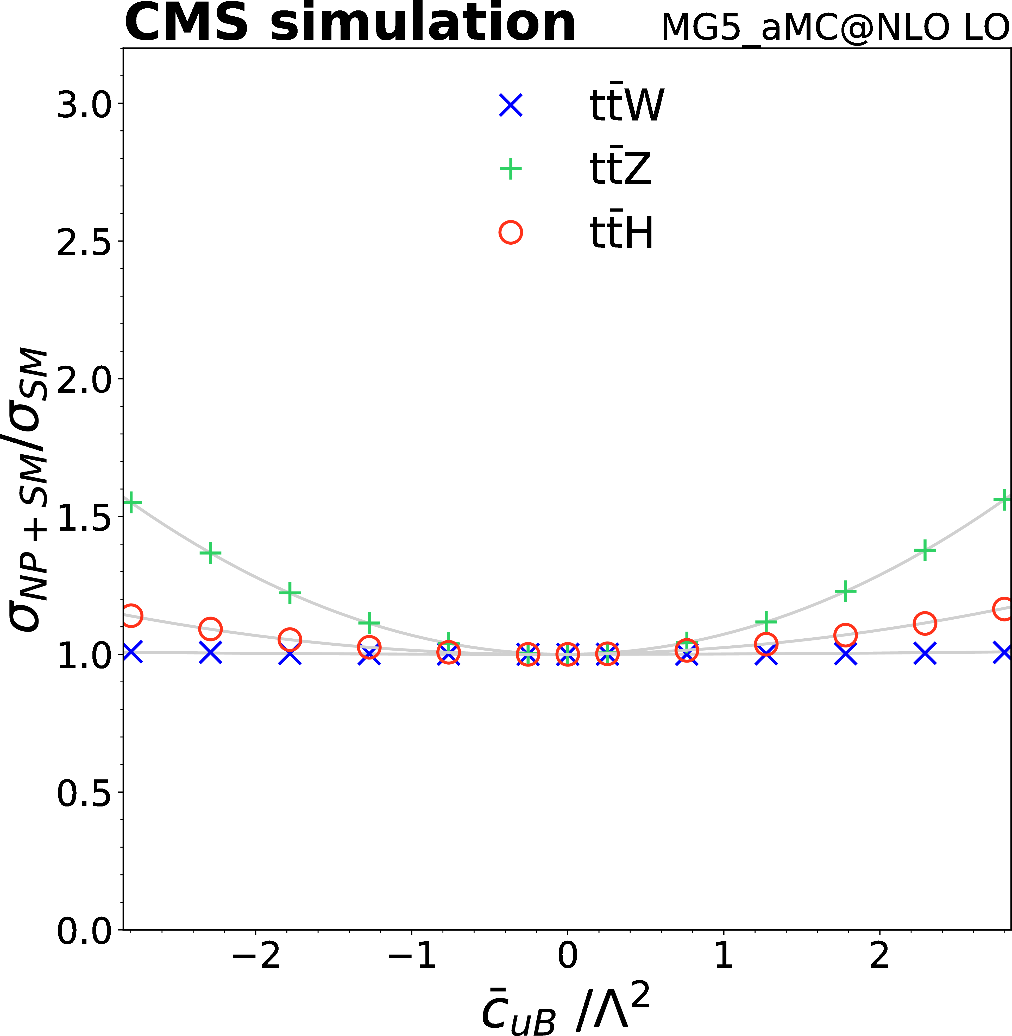
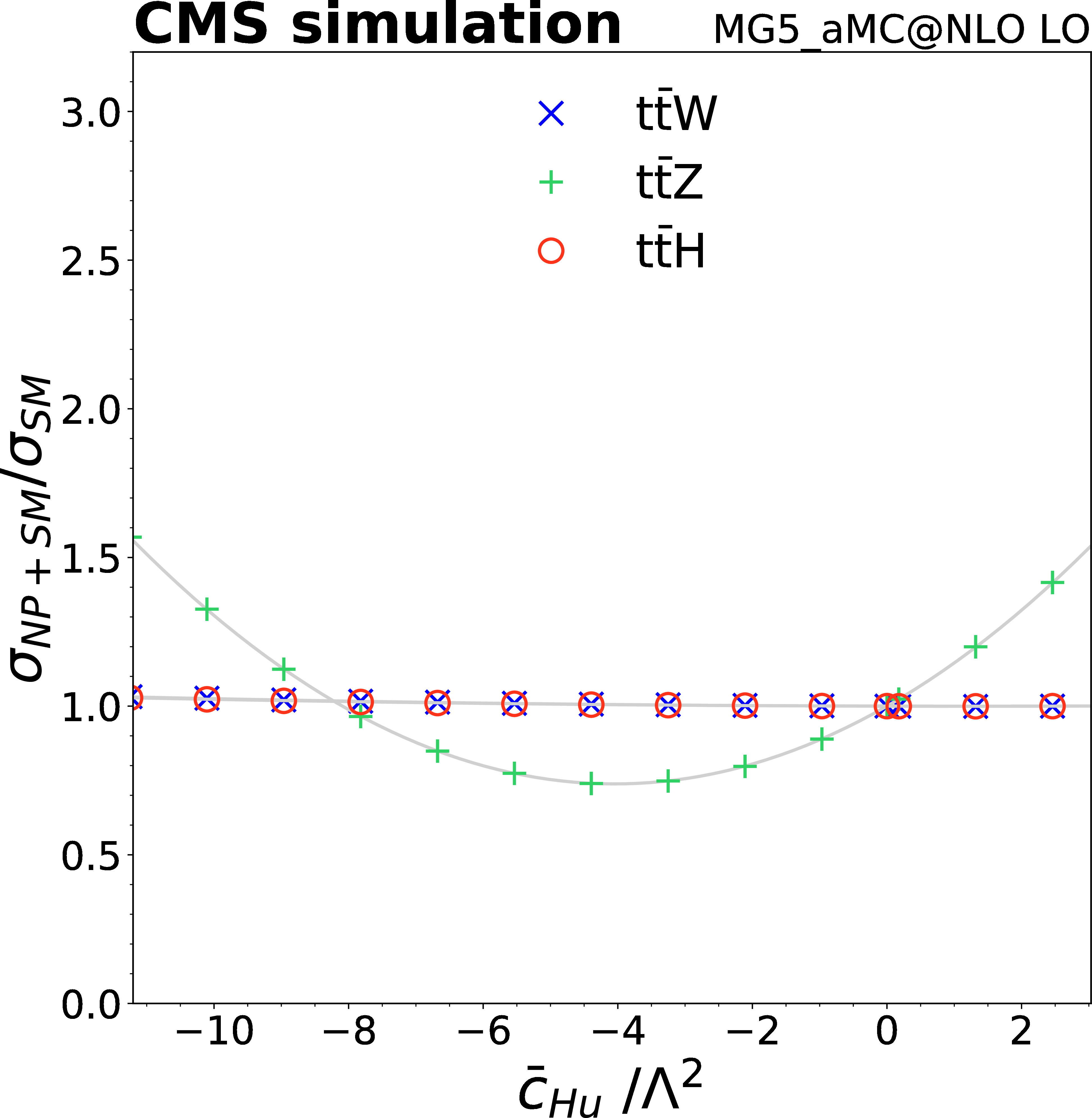
Figure 15:
Signal strength as a function of $c_j$ for $ {\bar{c}_{uW}} $ (top left), $ {\bar{c}_{u}} $ (top right), $ {\bar{c}_{uB}} $ (bottom left), and $ {\bar{c}_{Hu}} $ (bottom right). All three processes are affected by $ {\bar{c}_{uW}} $, while only $ {{\mathrm{ t } {}\mathrm{ \bar{t} } } \mathrm {H}} $ is affected by $ {\bar{c}_{u}} $ and only $ {{\mathrm{ t } {}\mathrm{ \bar{t} } } \mathrm{ Z } } $ is affected by $ {\bar{c}_{Hu}} $. Both $ {{\mathrm{ t } {}\mathrm{ \bar{t} } } \mathrm{ Z } } $ and $ {{\mathrm{ t } {}\mathrm{ \bar{t} } } \mathrm {H}} $ are sensitive to $ {\bar{c}_{uB}} $. |
png pdf |
Figure 15-a:
Signal strength as a function of $c_j$ for $ {\bar{c}_{uW}} $. All three processes are affected by $ {\bar{c}_{uW}} $. |

png pdf |
Figure 15-b:
Signal strength as a function of $c_j$ for $ {\bar{c}_{u}} $. Only $ {{\mathrm{ t } {}\mathrm{ \bar{t} } } \mathrm {H}} $ is affected by $ {\bar{c}_{u}} $. |
png pdf |
Figure 15-c:
Signal strength as a function of $c_j$ for $ {\bar{c}_{uB}} $. Both $ {{\mathrm{ t } {}\mathrm{ \bar{t} } } \mathrm{ Z } } $ and $ {{\mathrm{ t } {}\mathrm{ \bar{t} } } \mathrm {H}} $ are sensitive to $ {\bar{c}_{uB}} $. |
png pdf |
Figure 15-d:
Signal strength as a function of $c_j$ for $ {\bar{c}_{Hu}} $. Only $ {{\mathrm{ t } {}\mathrm{ \bar{t} } } \mathrm{ Z } } $ is affected by $ {\bar{c}_{Hu}} $. |

png pdf |
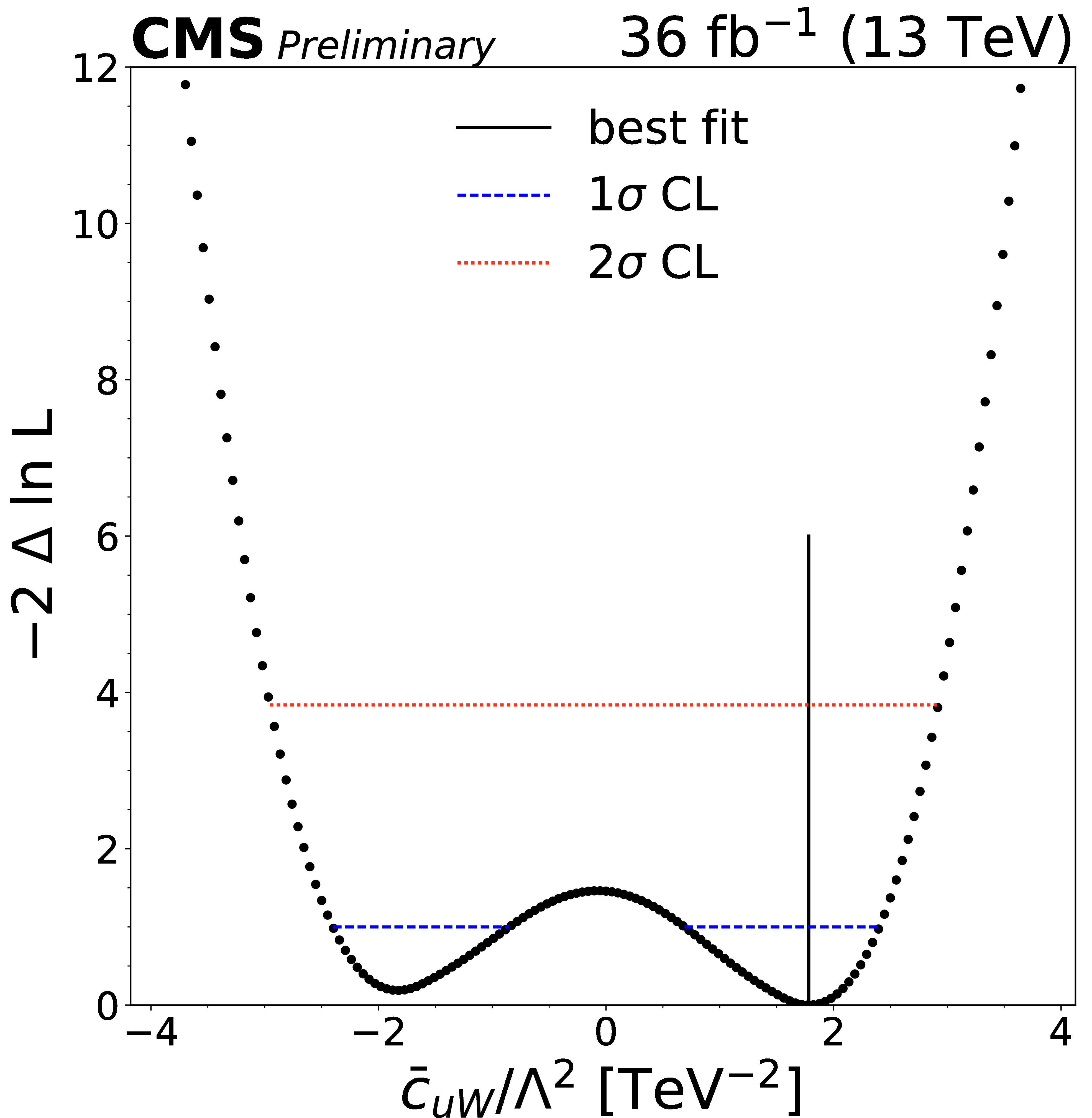
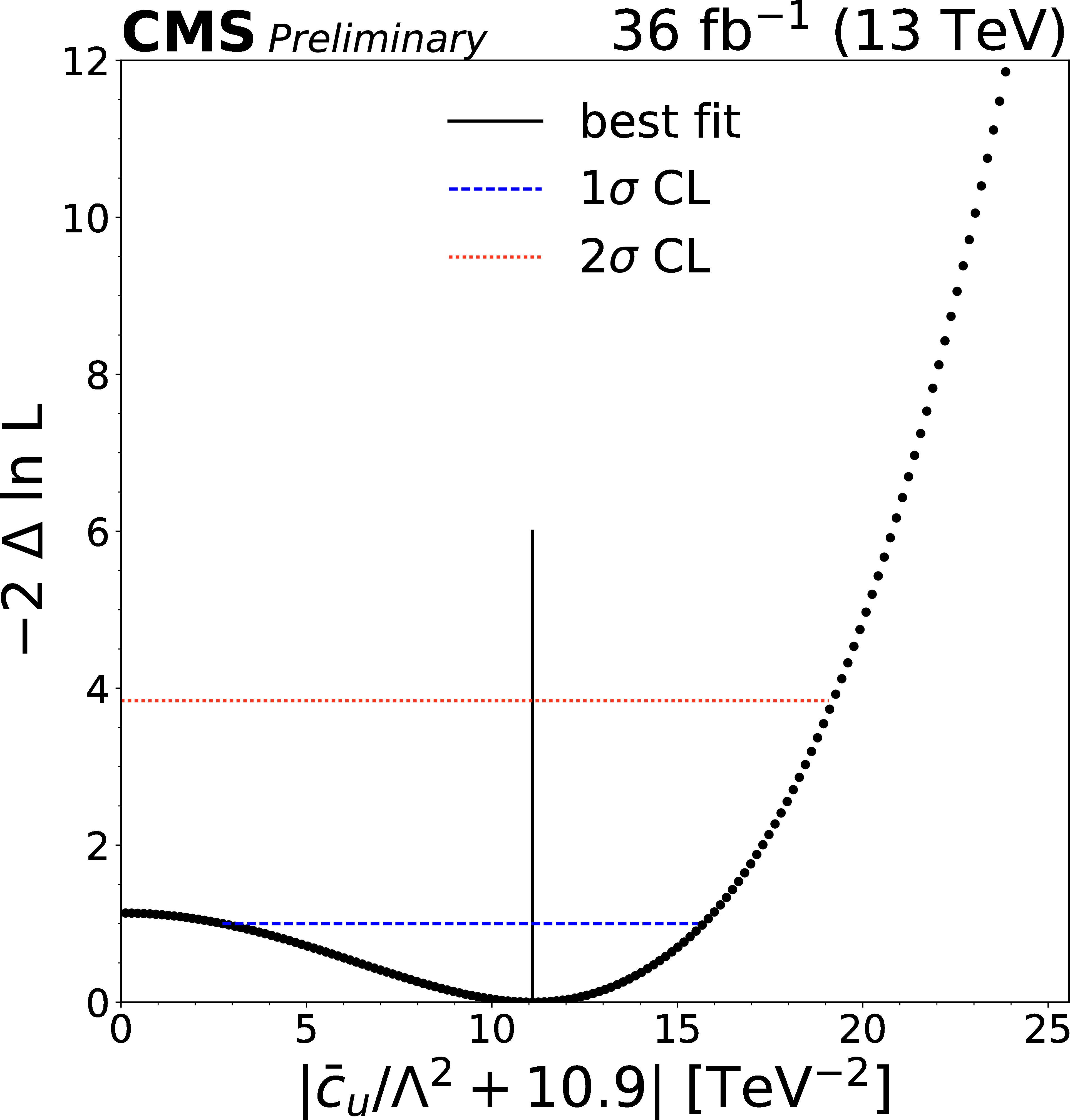
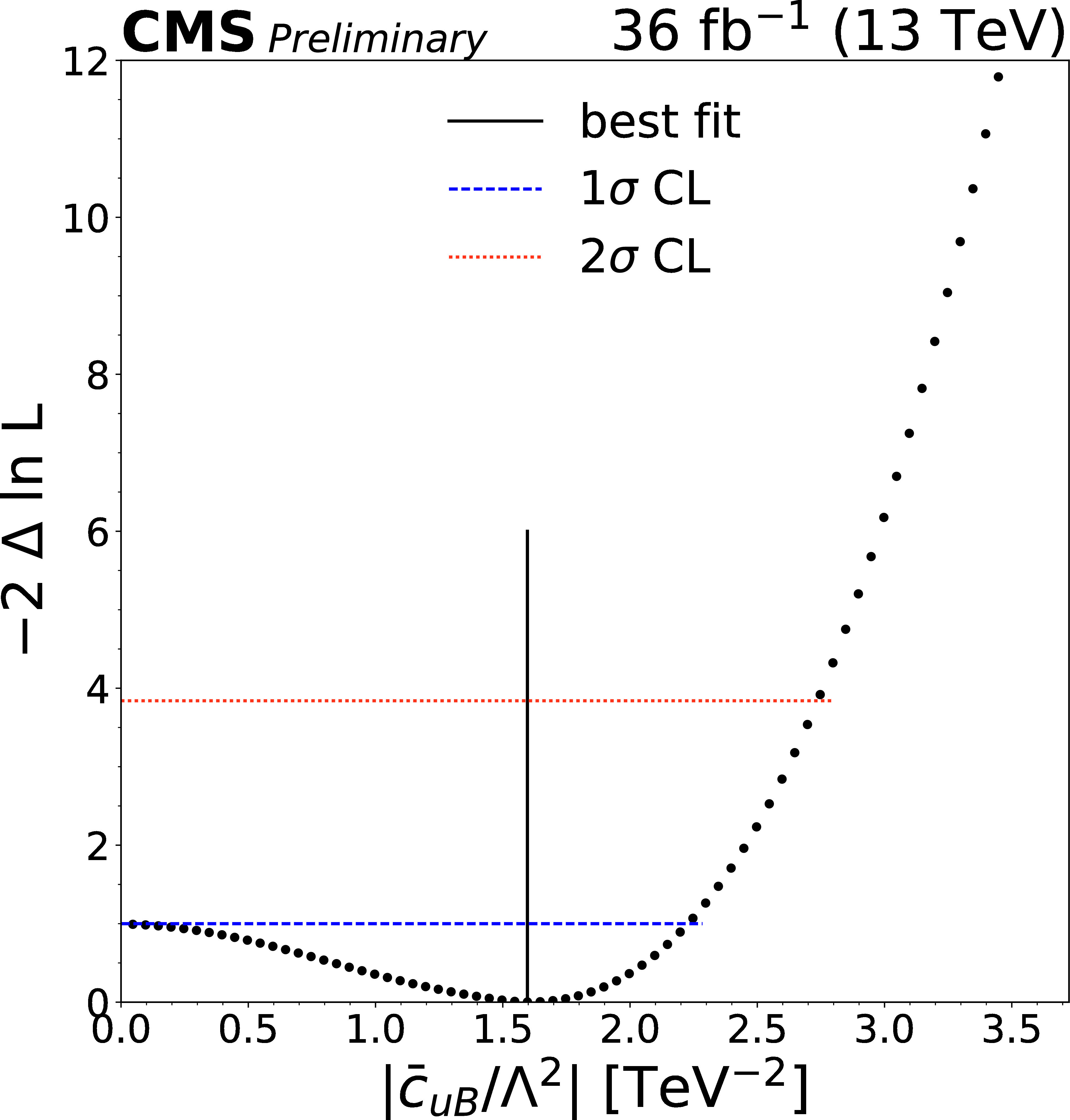
Figure 16:
The 1D test statistic $q(c_j)$ scan versus $c_j$, profiling all other nuisance parameters, for $ {\bar{c}_{uW}} $ (top left), $ {\bar{c}_{u}} $ (top right), $ {\bar{c}_{uB}} $ (bottom left), and $ {\bar{c}_{Hu}} $ (bottom right). The best-fit value is indicated by a solid line. Dotted lines and dashed lines indicate 1 $\sigma $ CLs and 2 $\sigma $ CLs, respectively. |
png pdf |
Figure 16-a:
The 1D test statistic $q(c_j)$ scan versus $c_j$, profiling all other nuisance parameters, for $ {\bar{c}_{uW}} $. The best-fit value is indicated by a solid line. Dotted lines and dashed lines indicate 1 $\sigma $ CLs and 2 $\sigma $ CLs, respectively. |
png pdf |
Figure 16-b:
The 1D test statistic $q(c_j)$ scan versus $c_j$, profiling all other nuisance parameters, for $ {\bar{c}_{u}} $. The best-fit value is indicated by a solid line. Dotted lines and dashed lines indicate 1 $\sigma $ CLs and 2 $\sigma $ CLs, respectively. |
png pdf |
Figure 16-c:
The 1D test statistic $q(c_j)$ scan versus $c_j$, profiling all other nuisance parameters, for $ {\bar{c}_{uB}} $. The best-fit value is indicated by a solid line. Dotted lines and dashed lines indicate 1 $\sigma $ CLs and 2 $\sigma $ CLs, respectively. |

png pdf |
Figure 16-d:
The 1D test statistic $q(c_j)$ scan versus $c_j$, profiling all other nuisance parameters, for $ {\bar{c}_{Hu}} $. The best-fit value is indicated by a solid line. Dotted lines and dashed lines indicate 1 $\sigma $ CLs and 2 $\sigma $ CLs, respectively. |

png pdf |
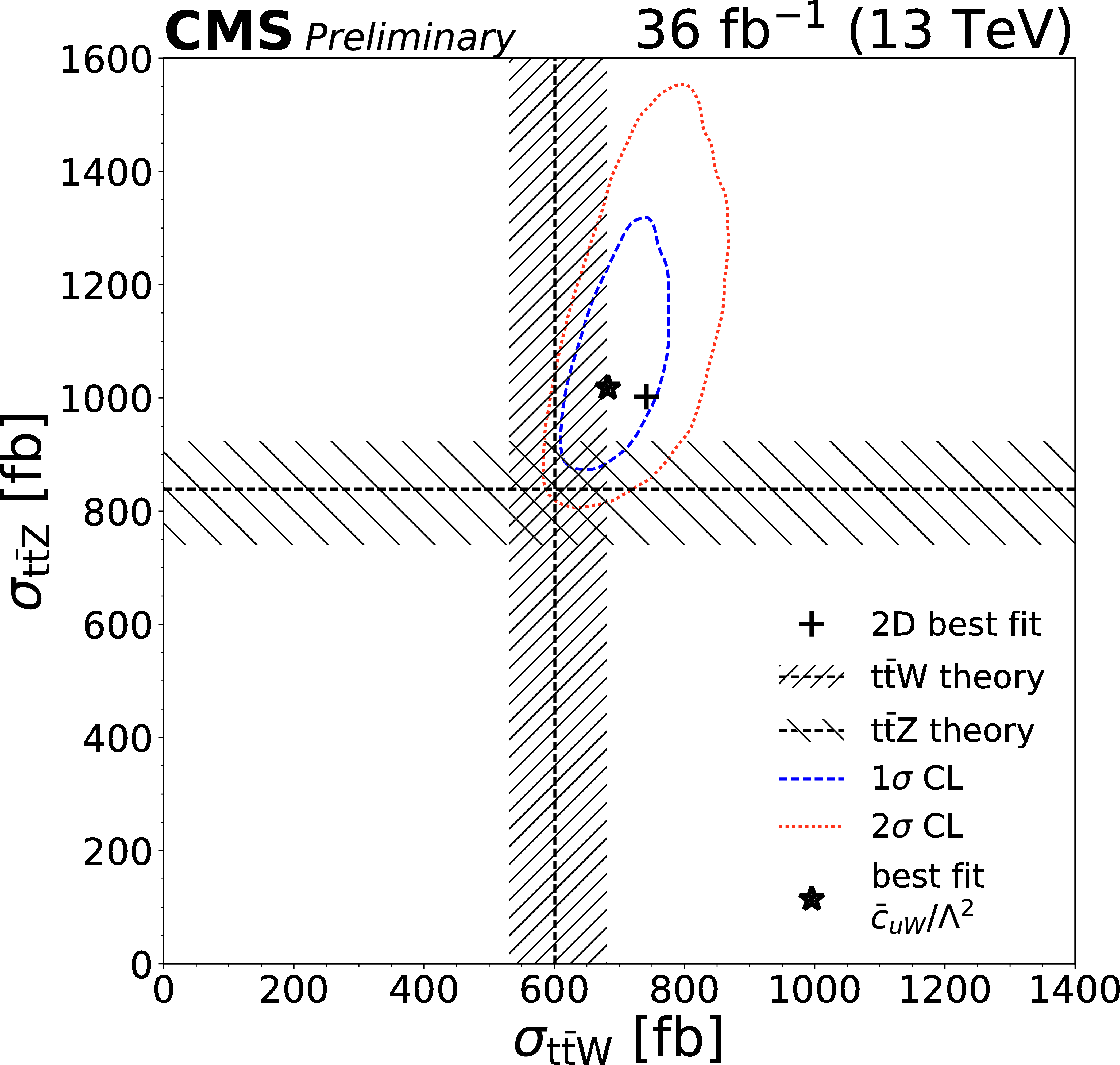
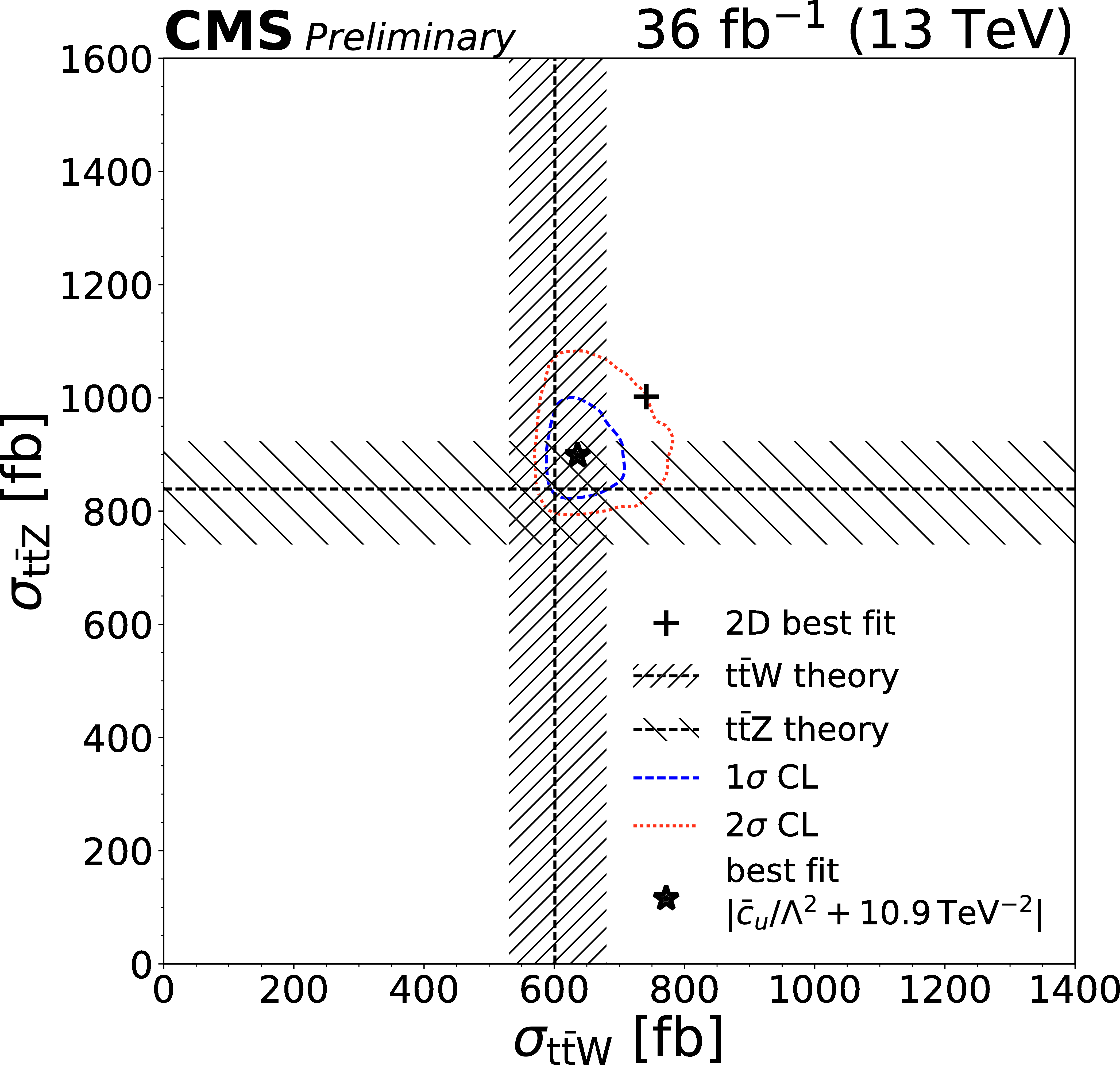
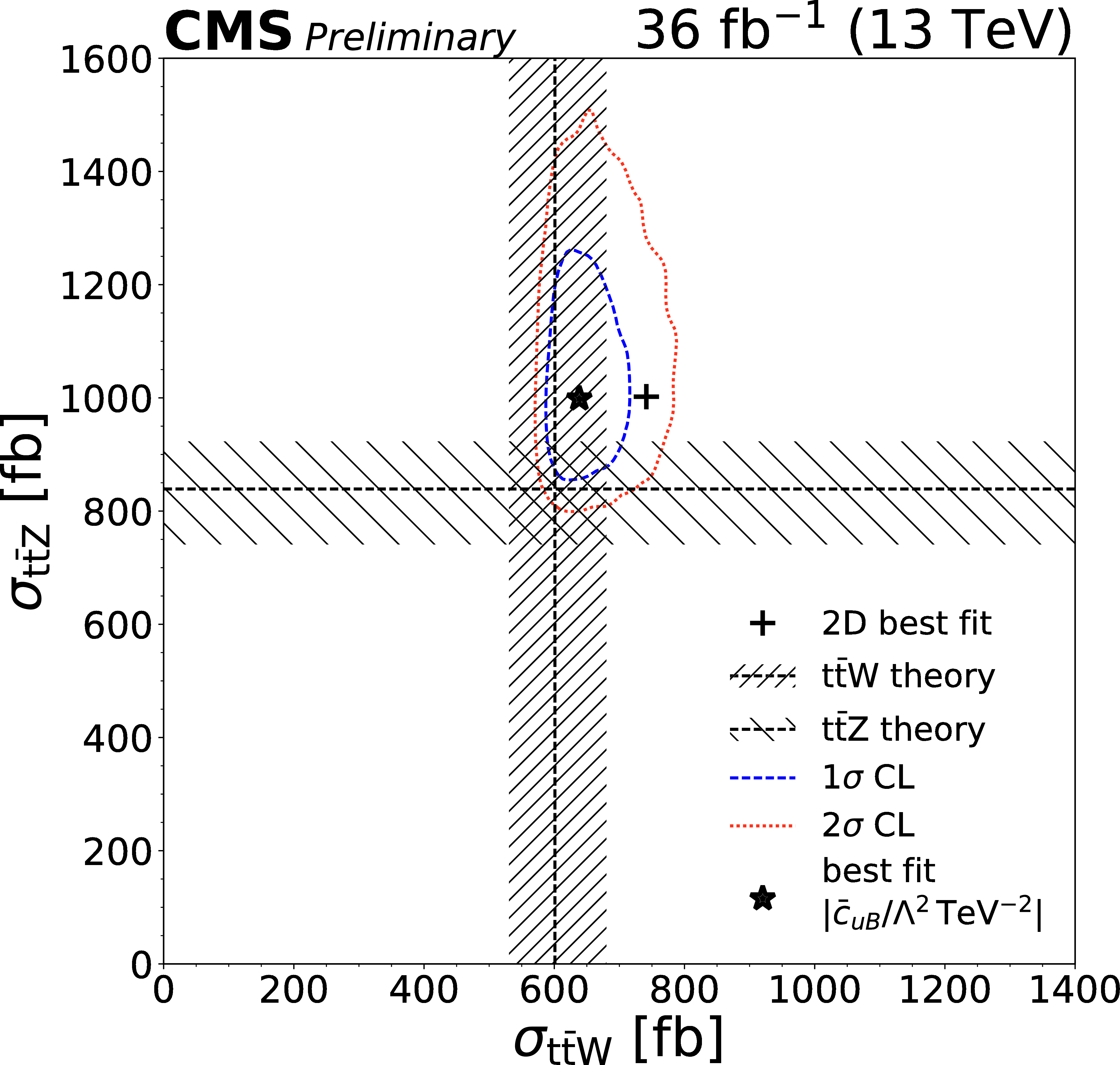
Figure 17:
The $ {{\mathrm{ t } {}\mathrm{ \bar{t} } } \mathrm{ Z } } $ and $ {{\mathrm{ t } {}\mathrm{ \bar{t} } } \mathrm{ W } } $ cross section corresponding to the best-fit value of $ {\bar{c}_{uW}} $ (top left), $ {\bar{c}_{u}} $ (top right), $ {\bar{c}_{uB}} $ (bottom left), and $ {\bar{c}_{Hu}} $ (bottom right) is shown as a star, along with the corresponding 1$\sigma $ (red) and 2$\sigma $ (blue) contours. The two-dimensional best fit to the $ {{\mathrm{ t } {}\mathrm{ \bar{t} } } \mathrm{ W } } $ and $ {{\mathrm{ t } {}\mathrm{ \bar{t} } } \mathrm{ Z } } $ cross sections is shown as a cross symbol. Predictions from theory at NLO (dotted lines) and their uncertanties (hatches) are also shown. |
png pdf |
Figure 17-a:
The $ {{\mathrm{ t } {}\mathrm{ \bar{t} } } \mathrm{ Z } } $ and $ {{\mathrm{ t } {}\mathrm{ \bar{t} } } \mathrm{ W } } $ cross section corresponding to the best-fit value of $ {\bar{c}_{uW}} $ is shown as a star, along with the corresponding 1$\sigma $ (red) and 2$\sigma $ (blue) contours. The two-dimensional best fit to the $ {{\mathrm{ t } {}\mathrm{ \bar{t} } } \mathrm{ W } } $ and $ {{\mathrm{ t } {}\mathrm{ \bar{t} } } \mathrm{ Z } } $ cross sections is shown as a cross symbol. Predictions from theory at NLO (dotted lines) and their uncertanties (hatches) are also shown. |
png pdf |
Figure 17-b:
The $ {{\mathrm{ t } {}\mathrm{ \bar{t} } } \mathrm{ Z } } $ and $ {{\mathrm{ t } {}\mathrm{ \bar{t} } } \mathrm{ W } } $ cross section corresponding to the best-fit value of $ {\bar{c}_{u}} $ is shown as a star, along with the corresponding 1$\sigma $ (red) and 2$\sigma $ (blue) contours. The two-dimensional best fit to the $ {{\mathrm{ t } {}\mathrm{ \bar{t} } } \mathrm{ W } } $ and $ {{\mathrm{ t } {}\mathrm{ \bar{t} } } \mathrm{ Z } } $ cross sections is shown as a cross symbol. Predictions from theory at NLO (dotted lines) and their uncertanties (hatches) are also shown. |
png pdf |
Figure 17-c:
The $ {{\mathrm{ t } {}\mathrm{ \bar{t} } } \mathrm{ Z } } $ and $ {{\mathrm{ t } {}\mathrm{ \bar{t} } } \mathrm{ W } } $ cross section corresponding to the best-fit value of $ {\bar{c}_{uB}} $ is shown as a star, along with the corresponding 1$\sigma $ (red) and 2$\sigma $ (blue) contours. The two-dimensional best fit to the $ {{\mathrm{ t } {}\mathrm{ \bar{t} } } \mathrm{ W } } $ and $ {{\mathrm{ t } {}\mathrm{ \bar{t} } } \mathrm{ Z } } $ cross sections is shown as a cross symbol. Predictions from theory at NLO (dotted lines) and their uncertanties (hatches) are also shown. |
png pdf |
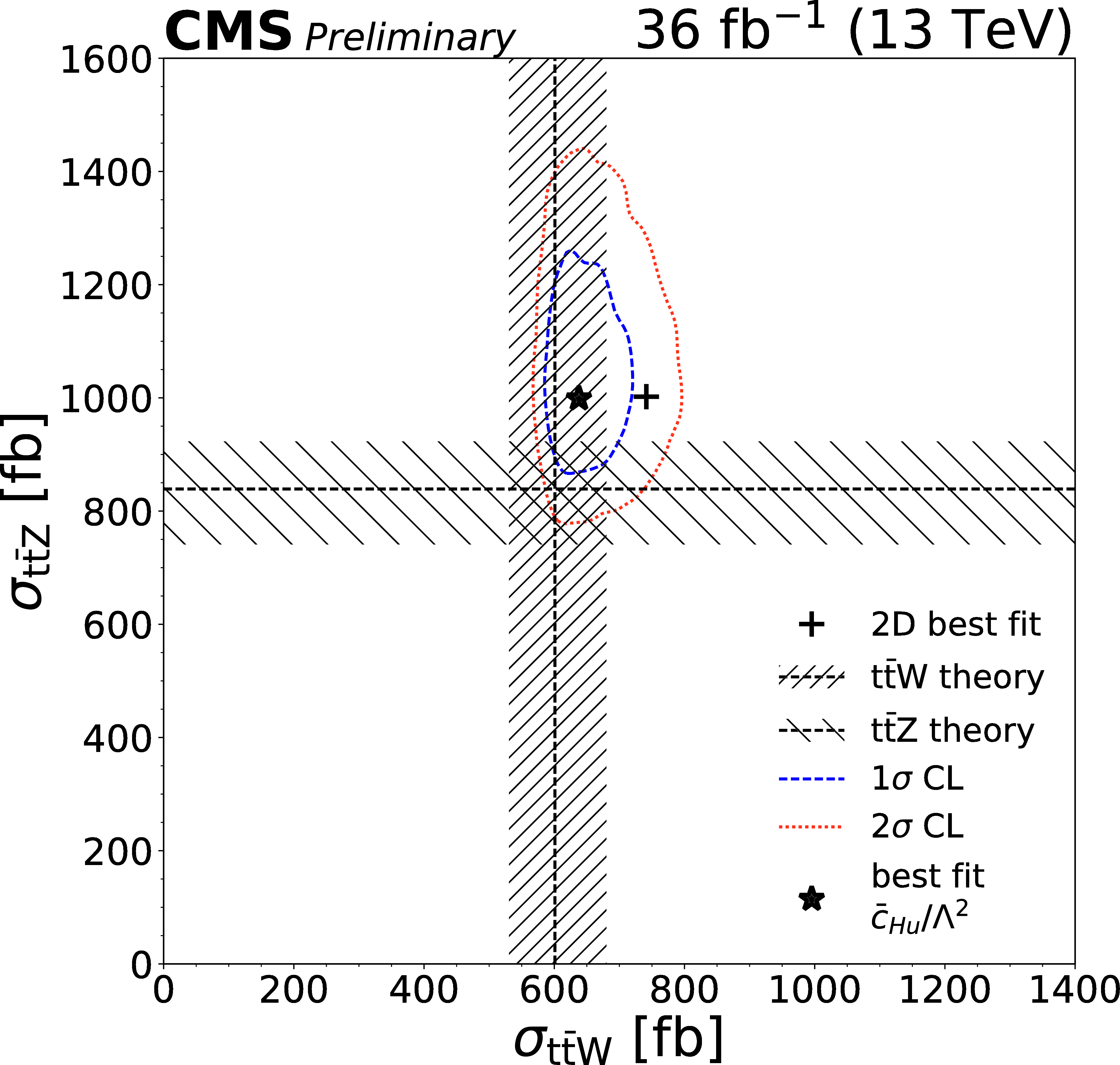
Figure 17-d:
The $ {{\mathrm{ t } {}\mathrm{ \bar{t} } } \mathrm{ Z } } $ and $ {{\mathrm{ t } {}\mathrm{ \bar{t} } } \mathrm{ W } } $ cross section corresponding to the best-fit value of $ {\bar{c}_{Hu}} $ is shown as a star, along with the corresponding 1$\sigma $ (red) and 2$\sigma $ (blue) contours. The two-dimensional best fit to the $ {{\mathrm{ t } {}\mathrm{ \bar{t} } } \mathrm{ W } } $ and $ {{\mathrm{ t } {}\mathrm{ \bar{t} } } \mathrm{ Z } } $ cross sections is shown as a cross symbol. Predictions from theory at NLO (dotted lines) and their uncertanties (hatches) are also shown. |
| Tables | |
png pdf |
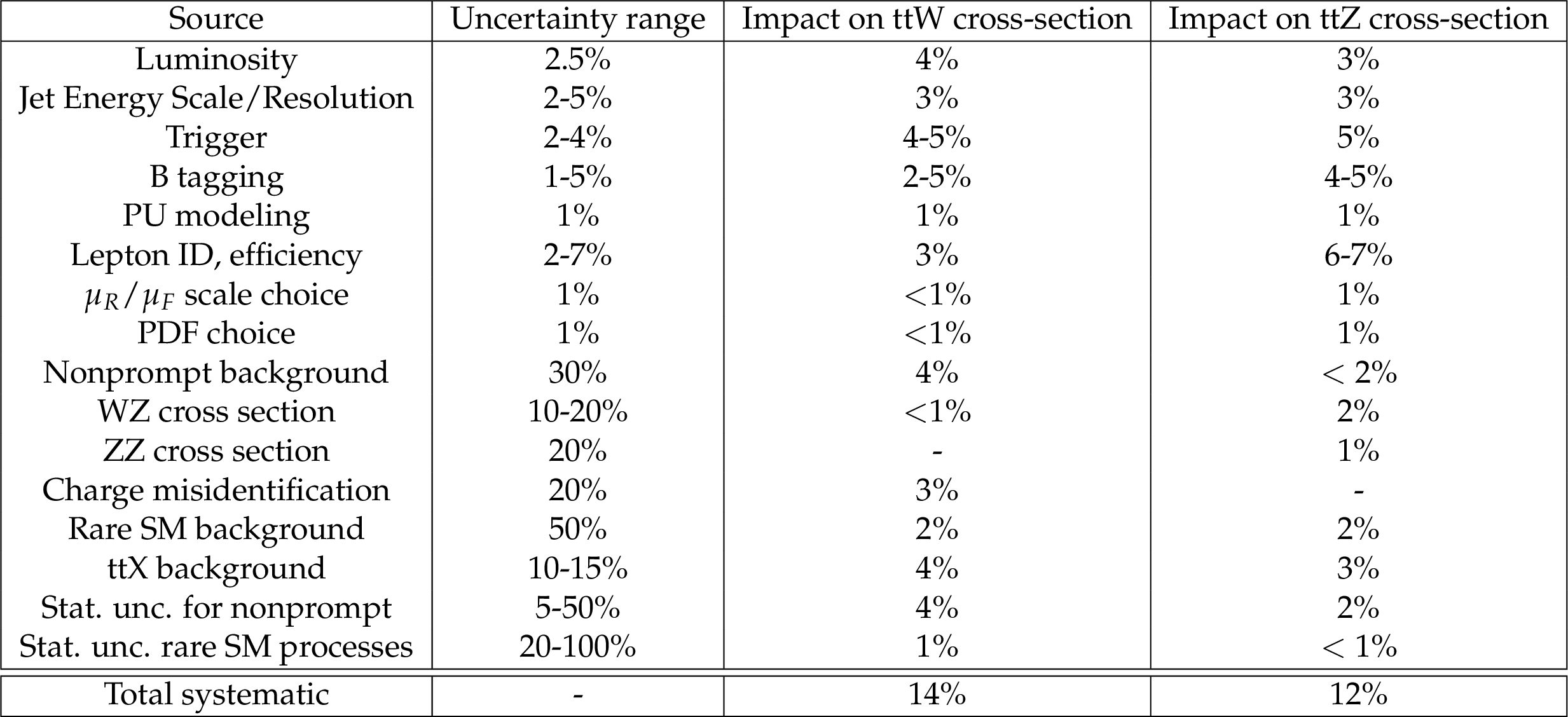
Table 1:
Summary of the sources of uncertainties, their magnitudes and effects. The first column shows the input uncertainty on each background and signal, while the second and third columns are the postfit uncertainties on ${{\mathrm{ t } {}\mathrm{ \bar{t} } } \mathrm{ W } }$ and ${{\mathrm{ t } {}\mathrm{ \bar{t} } } \mathrm{ Z } } $ cross-section measurements respectively. |
png pdf |
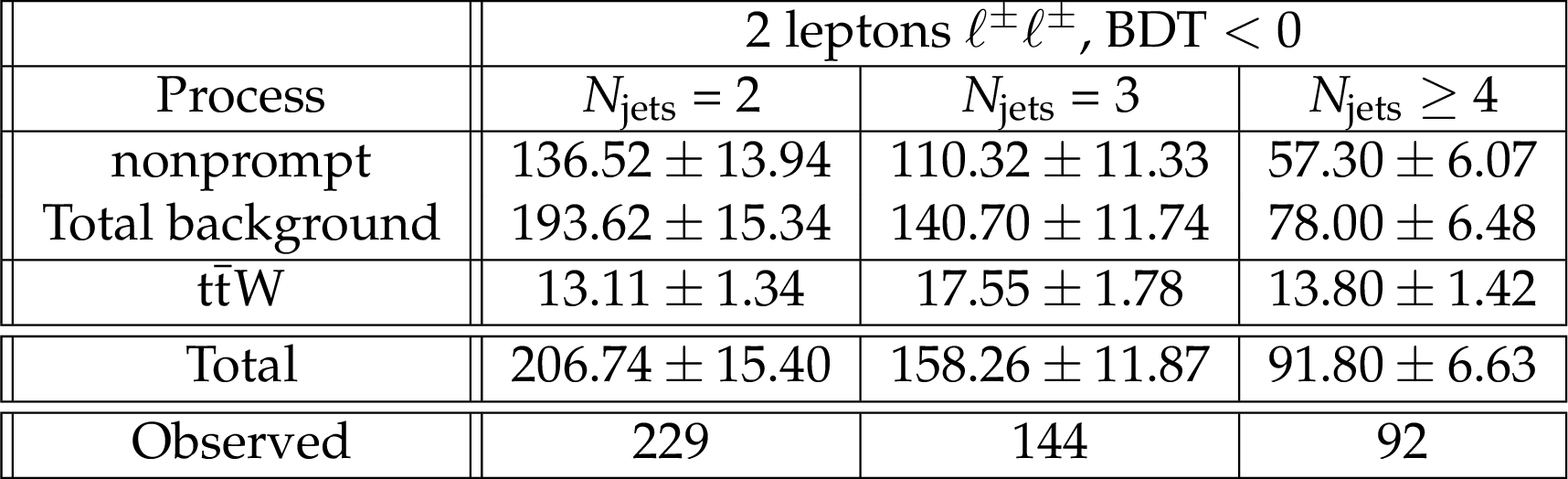
Table 2:
Post-fit predicted and observed yields in same-sign dilepton final state for BDT $<$ 0 region, i.e. nonprompt control region. The uncertainty represents the total post-fit uncertainty. |
png pdf |
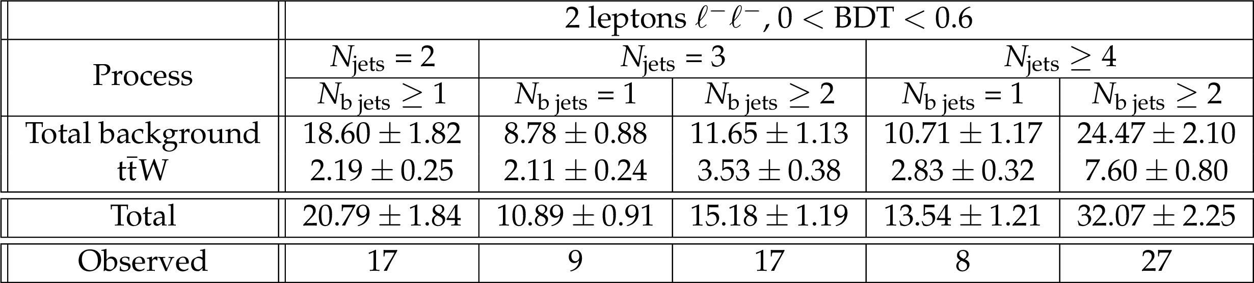
Table 3:
Post-fit predicted and observed yields in same-sign dilepton final state for 0 $<$ BDT $<$ 0.6 region where the sign of both leptons are negative. The uncertainty represents the total post-fit uncertainty. |
png pdf |
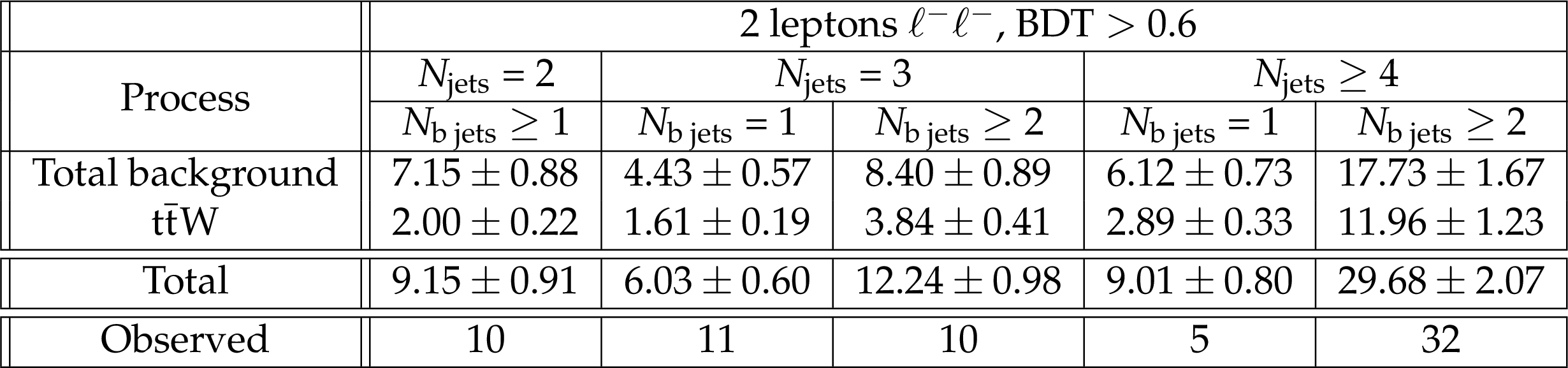
Table 4:
Post-fit predicted and observed yields in same-sign dilepton final state for BDT $>$ 0.6 region where the sign of both leptons are negative. The uncertainty represents the total post-fit uncertainty. |
png pdf |
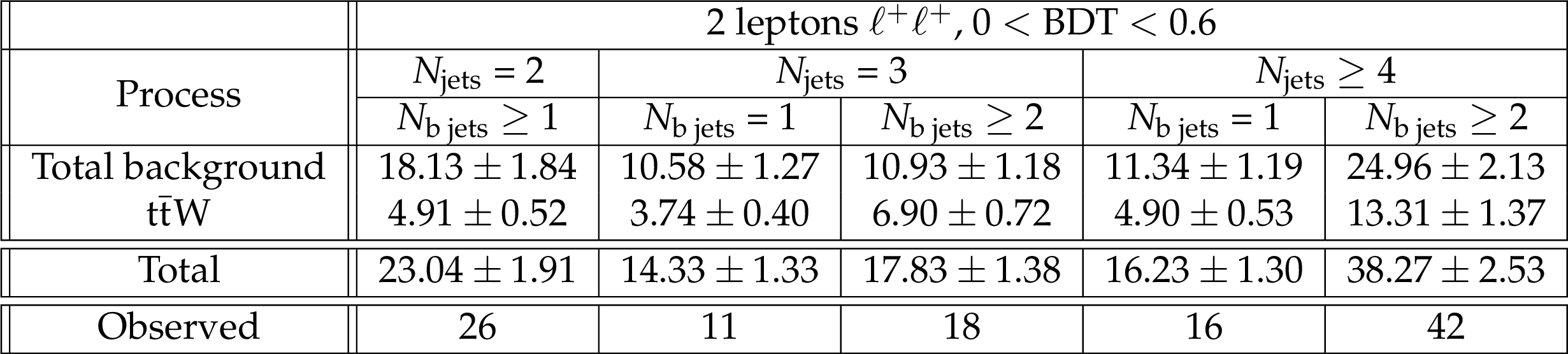
Table 5:
Post-fit predicted and observed yields in same-sign dilepton final state for 0 $<$ BDT $<$ 0.6 region where the sign of both leptons are positive. The uncertainty represents the total post-fit uncertainty. |
png pdf |
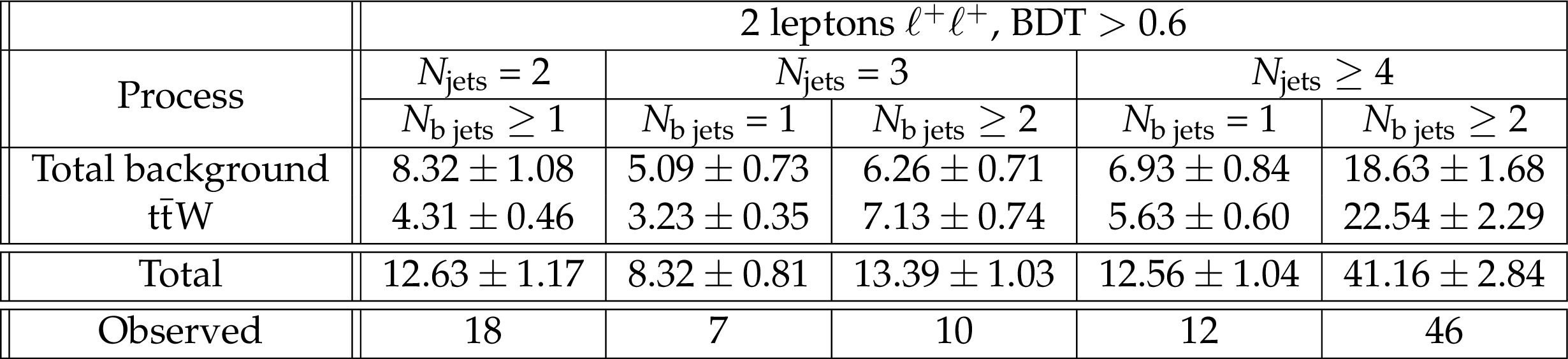
Table 6:
Post-fit predicted and observed yields in same-sign dilepton final state for BDT $>$ 0.6 region where the sign of both leptons are positive. The uncertainty represents the total post-fit uncertainty. |
png pdf |
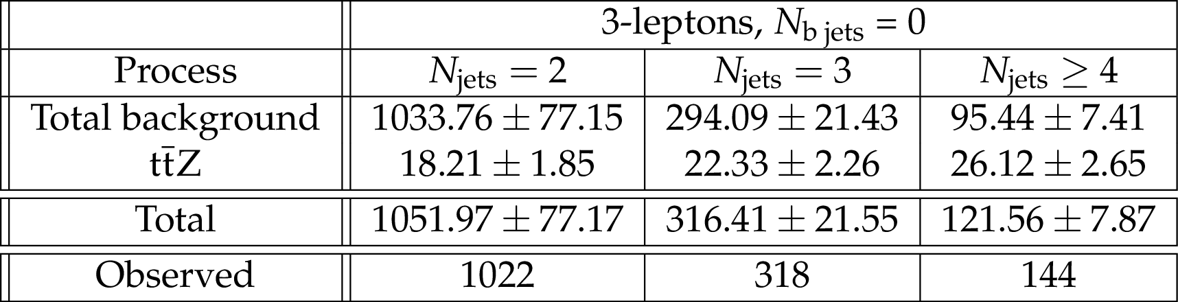
Table 7:
Post-fit predicted and observed yields in three-lepton final state in $ {N_\text {bjets}} = $ 0 category. The uncertainty represents the total post-fit uncertainty. |
png pdf |
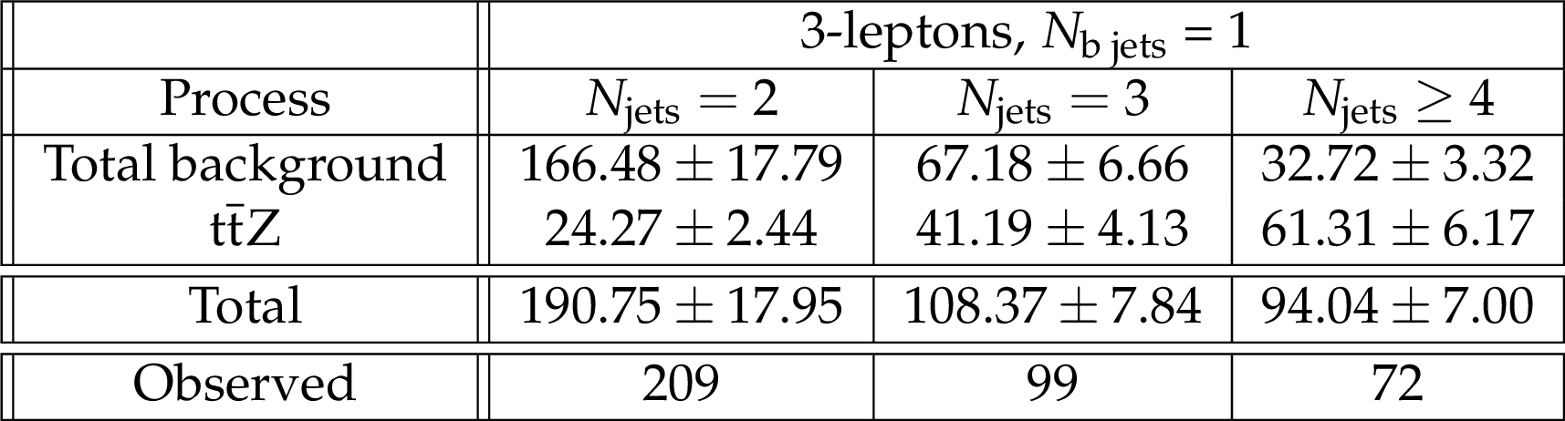
Table 8:
Post-fit predicted and observed yields in three-lepton final state in $ {N_\text {bjets}} = $ 1 category. The uncertainty represents the total post-fit uncertainty. |
png pdf |
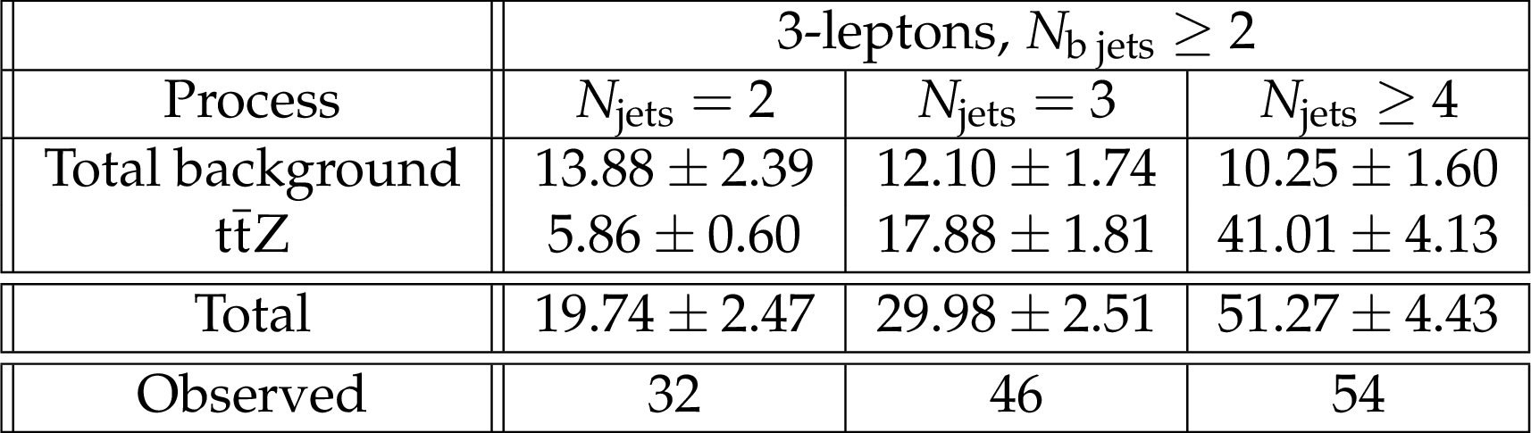
Table 9:
Post-fit predicted and observed yields in three-lepton final state in ${N_\text {bjets}} \geq $ 2 category. The uncertainty represents the total post-fit uncertainty. |
png pdf |
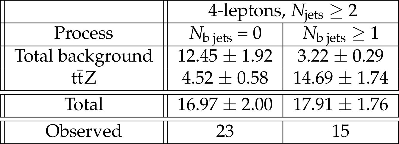
Table 10:
Post-fit predicted and observed yields in four-lepton final state. The uncertainty represents the total post-fit uncertainty. |
png pdf |
Table 11:
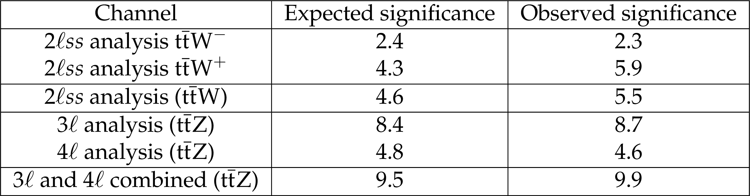
Summary of expected and observed significance for ${{\mathrm{ t } {}\mathrm{ \bar{t} } } \mathrm{ W } }$ in the same-sign 2-lepton channel and for ${{\mathrm{ t } {}\mathrm{ \bar{t} } } \mathrm{ Z } }$ in the 3-lepton, 4-lepton channels and in the two channels combined. |
png pdf |
Table 12:
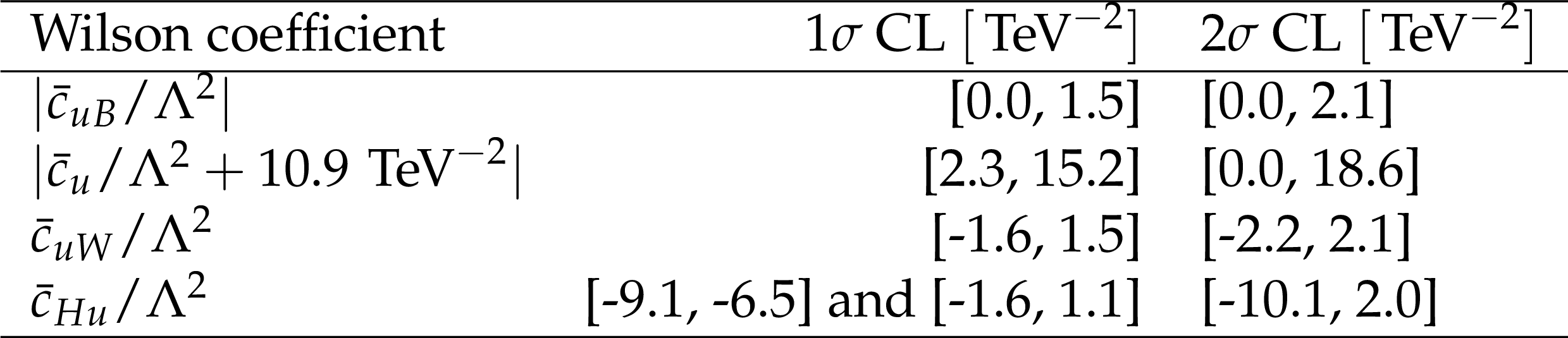
Expected 1$\sigma $ and 2$\sigma $ CL for this $ {{\mathrm{ t } {}\mathrm{ \bar{t} } } \mathrm{ W } } $ and $ {{\mathrm{ t } {}\mathrm{ \bar{t} } } \mathrm{ Z } } $ measurement, for selected Wilson coefficients. |
png pdf |
Table 13:
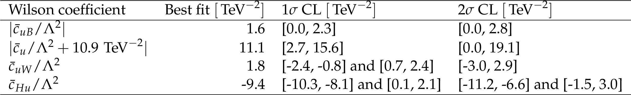
Observed best-fit values determined from this $ {{\mathrm{ t } {}\mathrm{ \bar{t} } } \mathrm{ W } } $ and $ {{\mathrm{ t } {}\mathrm{ \bar{t} } } \mathrm{ Z } } $ measurement, along with corresponding 1$\sigma $ and 2$\sigma $ CL intervals for selected Wilson coefficients. |
| Summary |
| A measurement of top quark pair production in association with a W or a Z boson using 13 TeV data is presented. The analysis is performed in the same-sign dilepton final state for ${\mathrm{ t \bar{t} }\mathrm{ W }} $ and the three- and four-lepton final states for ${\mathrm{ t \bar{t} }\mathrm{ Z }} $, and these three are used to extract the cross sections of ${\mathrm{ t \bar{t} }\mathrm{ W }} $ and ${\mathrm{ t \bar{t} }\mathrm{ Z }} $ production. The same-sign dilepton channel achieves a significance of 5.5 standard deviations, the three-lepton analysis 8.7 standard deviations and the four-lepton analysis 4.6 standard deviatations. From the combination of three- and four-lepton channels a significance of 9.9 standard deviations for ${\mathrm{ t \bar{t} }\mathrm{ Z }} $ is obtained. The measured cross sections are $\sigma({\mathrm{ t \bar{t} }\mathrm{ Z }} )= $ 1.00$^{+0.09}_{-0.08}$ (stat.) $^{+0.12}_{-0.10} $ (sys.) pb and $\sigma({\mathrm{ t \bar{t} }\mathrm{ W }} )= $ 0.80$^{+0.12}_{-0.11}$ (stat.) $^{+0.13}_{-0.12} $ (sys.) pb, in agreement with the standard model predictions. These results have been used to set constraints on the Wilson coefficients of four operators which would modify $\mathrm{t\overline{t}Z}$ and $\mathrm{t\overline{t}W}$ production. |
| References | ||||
| 1 | B. Mellado Garcia, P. Musella, M. Grazzini, and R. Harlander | CERN Report 4: Part I Standard Model Predictions | Technical Report LHCHXSWG-DRAFT-INT-2016-008 | |
| 2 | CMS Collaboration | The CMS experiment at the CERN LHC | JINST 3 (2008) S08004 | CMS-00-001 |
| 3 | CMS Collaboration | Measurement of associated production of vector bosons and $ \mathrm{ t \bar{t} } $ in pp collisions at $ \sqrt{s} = $ 7 TeV | PRL 110 (2013) 172002 | CMS-TOP-12-014 1303.3239 |
| 4 | CMS Collaboration | Measurement of top quark-antiquark pair production in association with a W or Z boson in pp collisions at $ \sqrt{s} = $ 8 TeV | Eur. Phys. J.C 74 (2014), no. 9 | CMS-TOP-12-036 1406.7830 |
| 5 | CMS Collaboration | Observation of top quark pairs produced in association with a vector boson in pp collisions at $ \sqrt{s} = $ 8 TeV | JHEP 01 (2016) 096 | CMS-TOP-14-021 1510.01131 |
| 6 | ATLAS Collaboration | Measurement of the $ t\overline{t}W $ and $ t\overline{t}Z $ production cross sections in pp collisions at $ \sqrt{s} = $ 8 TeV with the ATLAS detector | JHEP 11 (2015) 172 | 1509.05276 |
| 7 | ATLAS Collaboration | Measurement of the $ t\overline{t}Z $ and $ t\overline{t}W $ production cross sections in multilepton final states using 3.2 $ fb^{-1} $ of pp collisions at $ \sqrt{s} = $ 13 TeV with the ATLAS detector | EPJC. | 1609.01599 |
| 8 | J. Alwall et al. | MadGraph 5 : Going Beyond | JHEP 06 (2011) 128 | 1106.0522 |
| 9 | S. Frixione and B. R. Webber | Matching NLO QCD computations and parton shower simulations | JHEP 06 (2002) 29 | hep-ph/0204244 |
| 10 | T. Sjostrand, S. Mrenna, and P. Skands | PYTHIA 6.4 physics and manual | JHEP 05 (2006) 026 | hep-ph/0603175 |
| 11 | T. Sjostrand et al. | An Introduction to PYTHIA 8.2 | CPC 191 (2015) 159--177 | 1410.3012 |
| 12 | S. Alioli et al. | NLO single-top production matched with shower in POWHEG: $ s $- and $ t $-channel contributions | JHEP 09 (2009) 111 | 0907.4076 |
| 13 | S. Alioli et al. | A general framework for implementing NLO calculations in shower Monte Carlo programs: the POWHEG BOX | JHEP 06 (2010) 043 | 1002.2581 |
| 14 | J. M. Campbell and R. K. Ellis | MCFM for the Tevatron and the LHC | NPPS 205-206 (2010) 10--15 | 1007.3492 |
| 15 | F. Cascioli et al. | ZZ production at hadron colliders in NNLO QCD | PLB735 (2014) 311--313 | 1405.2219 |
| 16 | F. Caola, K. Melnikov, R. Rantsch, and L. Tancredi | QCD corrections to ZZ production in gluon fusion at the LHC | PRD92 (2015), no. 9, 094028 | 1509.06734 |
| 17 | GEANT4 Collaboration | Geant 4 -- a simulation toolkit | NIMA 506 (2003) 250 | |
| 18 | CMS Collaboration | Commissioning of the Particle-Flow Reconstruction in Minimum-Bias and Jet Events from pp Collisions at 7 TeV | CDS | |
| 19 | M. Cacciari, G. P. Salam, and G. Soyez | FastJet User Manual | EPJC 72 (2012) 1896 | 1111.6097 |
| 20 | M. Cacciari and G. P. Salam | Dispelling the $ N^{3} $ myth for the $ k_t $ jet-finder | PLB 641 (2006) 57--61 | hep-ph/0512210 |
| 21 | M. Cacciari, G. P. Salam, and G. Soyez | The anti-$ k_t $ jet clustering algorithm | JHEP 04 (2008) 063 | 0802.1189 |
| 22 | CMS Collaboration | Pileup Removal Algorithms | CMS-PAS-JME-14-001 | CMS-PAS-JME-14-001 |
| 23 | CMS Collaboration | Identification of b-quark jets with the CMS experiment | JINST 8 (2013) 04013 | CMS-BTV-12-001 1211.4462 |
| 24 | Particle Data Group | Review of particle physics | CPC 38 (2014) 090001 | |
| 25 | A. Hoecker, P. Speckmayer, J. Stelzer, J. Therhaag, E. von Toerne, H. Voss Collaboration | TMVA 4, Toolkit for Multivariate Data Analysis with ROOT, Users Guide | Technical Report CERN-OPEN-2007-007 | |
| 26 | CMS Collaboration | Search for new physics in same-sign dilepton events in proton-proton collisions at $ \sqrt{s} = $ 13 TeV | Eur. Phys. J.C (2016) , [Erratum: Eur. Phys. J.C76,439(2016)] | CMS-SUS-15-008 1605.03171 |
| 27 | J. Campbell, R. K. Ellis, and R. Rontsch | Single top production in association with a Z boson at the LHC | PRD 87 (2013) 114006 | 1302.3856 |
| 28 | S. Frixione et al. | Electroweak and QCD corrections to top-pair hadroproduction in association with heavy bosons | JHEP 06 (2015) 184 | 1504.03446 |
| 29 | J. Alwall et al. | The automated computation of tree-level and next-to-leading order differential cross sections, and their matching to parton shower simulations | JHEP 07 (2014) 079 | 1405.0301 |
| 30 | CMS Collaboration Collaboration | CMS Luminosity Measurements for the 2016 Data Taking Period | Technical Report CMS-PAS-LUM-17-001, CERN, Geneva | |
| 31 | CMS Collaboration | Performance of CMS muon reconstruction in pp collision events at $ \sqrt{s} = $ 7 TeV | JINST 7 (2012) P10002 | CMS-MUO-10-004 1206.4071 |
| 32 | CMS Collaboration | Performance of electron reconstruction and selection with the CMS detector in proton-proton collisions at $ \sqrt{s} = $ 8 TeV | JINST 10 (2015) P06005 | CMS-EGM-13-001 1502.02701 |
| 33 | CMS Collaboration | Identification of b-quark jets with the CMS experiment | JINST 8 (2013) P04013 | CMS-BTV-12-001 1211.4462 |
| 34 | NNPDF Collaboration | Parton distributions for the LHC Run II | JHEP 04 (2015) 040 | 1410.8849 |
| 35 | ATLAS and CMS Collaborations | Procedure for the LHC Higgs boson search combination in summer 2011 | ATL-PHYS-PUB-2011-011, CMS NOTE-2011/005 | |
| 36 | G. Cowan, K. Cranmer, E. Gross, and O. Vitells | Asymptotic formulae for likelihood-based tests of new physics | Eur. Phys. J.C 71 (2011) 1554, , [Erratum: Eur. Phys. J.C73,2501(2013)] | 1007.1727 |
| 37 | W. Buchmuller and D. Wyler | Effective lagrangian analysis of new interactions and flavour conservation | Nucl. Phys. B 268 (1986) 621--653 | |
| 38 | B. Grzadkowski, M. Iskrzynski, M. Misiak, and J. Rosiek | Dimension-Six Terms in the Standard Model Lagrangian | 1008.4884 | |
| 39 | A. Alloul, B. Fuks, and V. Sanz | Phenomenology of the Higgs effective Lagrangian via FeynRules | JHEP 2014 (April, 2014) 110 | 1310.5150 |
| 40 | J. Ellis, V. Sanz, and T. You | Complete Higgs Sector Constraints on Dimension-6 Operators | 1404.3667 | |
| 41 | K. Whisnant, J. M. Yang, B.-L. Young, and X. Zhang | Dimension-six CP-conserving operators of the third-family quarks and their effects on collider observables | 9702305 | |
| 42 | E. Berger, Q. Cao, and I. Low | Model independent constraints among the W tb, Z BOSON, and Z BOSON couplings | PRD (2009) 1--30 | 0907.2191v2 |
| 43 | R. Rontsch and M. Schulze | Constraining couplings of the top quarks to the Z boson in ttbar+Z production at the LHC | 1404.1005 | |
| 44 | E. Malkawi and C.-P. Yuan | Global analysis of the top quark couplings to gauge bosons | PRD 50 (Oct, 1994) 4462--4477 | |
| 45 | C. Zhang, N. Greiner, and S. Willenbrock | Constraints on nonstandard top quark couplings | PRD 86 (July, 2012) 014024 | |
| 46 | A. Tonero and R. Rosenfeld | Dipole-induced anomalous top quark couplings at the LHC | PRD 90 (July, 2014) 017701 | arXiv:1404.2581v2 |
| 47 | A. Alloul et al. | FeynRules 2.0 - A complete toolbox for tree-level phenomenology | 1310.1921 | |
|
|
Compact Muon Solenoid LHC, CERN |
|

|

|

|

|

|