CMS-PAS-SMP-23-006

CMS-PAS-SMP-23-006
Proton reconstruction using the TOTEM Roman pot detectors during the high- $\beta^*$ data taking period
CMS Collaboration
18 July 2024

Abstract: The TOTEM Roman pot detectors are used to reconstruct the transverse momentum of scattered protons and to estimate the transverse location of the primary interaction. In this study advanced methods of local track reconstruction, measurements of strip-level detection efficiencies, cross-checks of beam optics, and detector alignment techniques are presented, along with their application in the selection of signal collision events. The local track reconstruction is performed by exploiting hit cluster information through a novel method, by finding a common polygonal area in the intercept-slope plane. The tool is applied in the relative alignment of detector layers with $\mu$ m precision. A tag-and-probe method is used to extract strip-level detection efficiencies. The proton reconstruction corrections are calculated using a simulation. The absolute alignment of the Roman pot system is performed through several measured quantities. The necessary run-by-run adjustments are in the range $\pm$ 50 $\mu$ m in horizontal, and $\pm$ 0.5 mm in vertical directions. The goal is to provide a solid ground for exclusive physics analyses based on the high- $\beta^*$ data taking period in 2018.
Links: CDS record (PDF) ; CADI line (restricted) ; These preliminary results are superseded in this paper, Submitted to JINST. The superseded preliminary plots can be found here.

Figures & Tables	Summary	References	CMS Publications

Figures
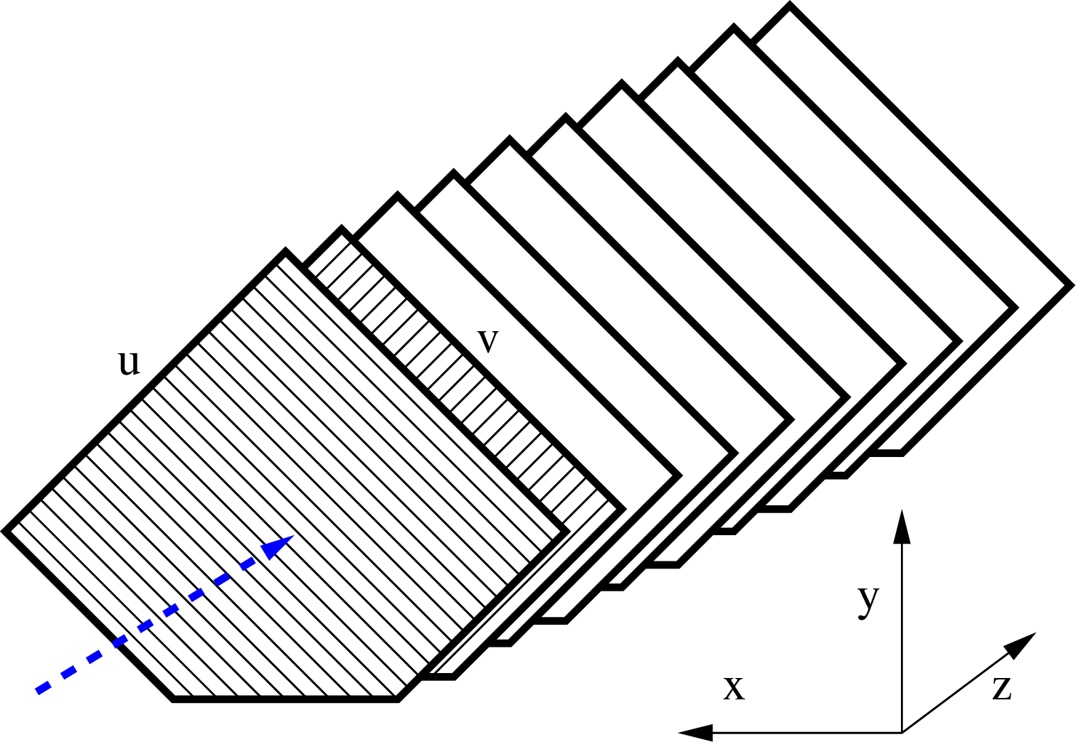
png pdf	Figure 1: Schematic drawing of a RP unit: 10 layers with strips oriented alternately in u and v directions are shown. The blue dashed arrow represents an incoming proton. The axes of the local coordinate system are indicated with black arrows.
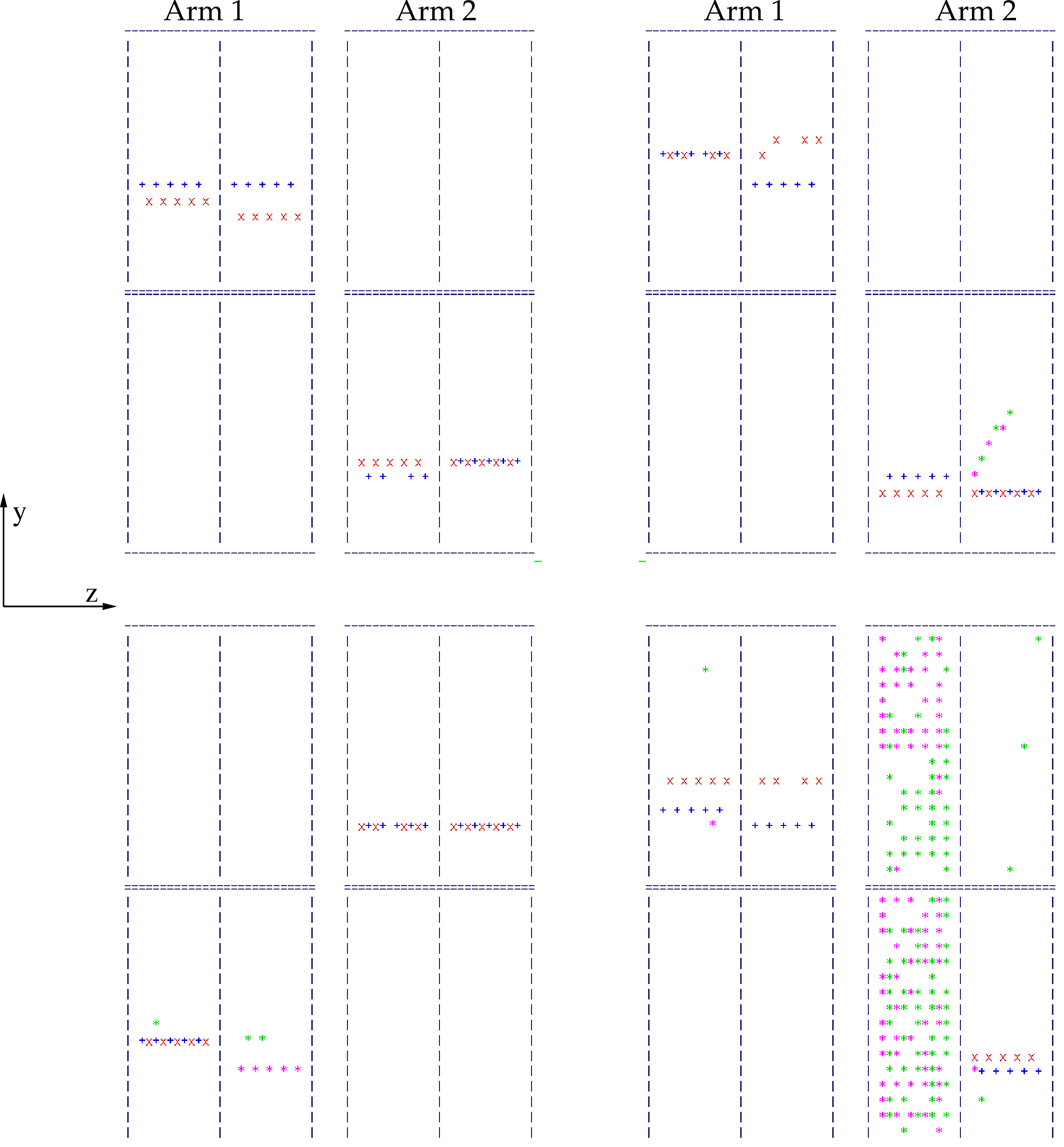
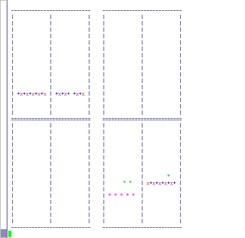
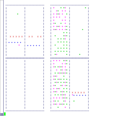
png pdf	Figure 2: Schematic displays of four events with hits and projections of reconstructed local tracks (tracklets) in RPs, not to scale. Outlines of Arm 1 and 2, near and far, top and bottom plots are drawn. Reconstructed clusters on a found tracklet are plotted, on u layers (red) and v layers (blue). Reconstructed clusters not on a found tracklet are plotted with green or magenta $\ast$ symbols. From left to right and from top to bottom: normal, normal with secondary; not reconstructed (less than three hits in v orientation of 1n); not reconstructed (hadronic interaction in some beam element before 2n).
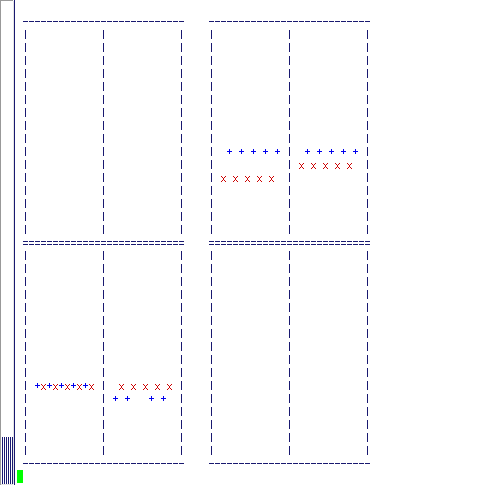
png	Figure 2-a: Schematic displays of four events with hits and projections of reconstructed local tracks (tracklets) in RPs, not to scale. Outlines of Arm 1 and 2, near and far, top and bottom plots are drawn. Reconstructed clusters on a found tracklet are plotted, on u layers (red) and v layers (blue). Reconstructed clusters not on a found tracklet are plotted with green or magenta $\ast$ symbols. From left to right and from top to bottom: normal, normal with secondary; not reconstructed (less than three hits in v orientation of 1n); not reconstructed (hadronic interaction in some beam element before 2n).
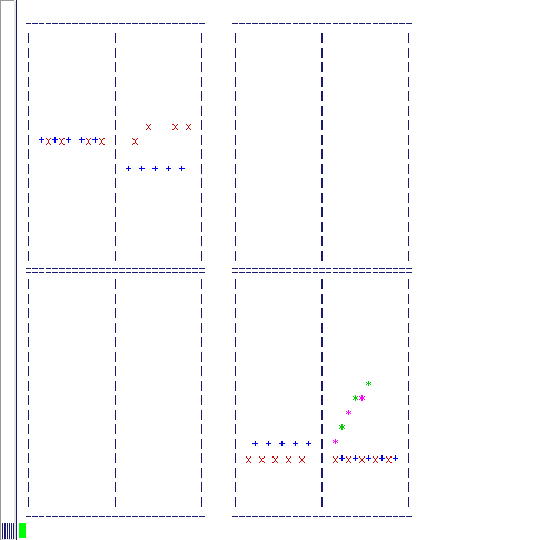
png	Figure 2-b: Schematic displays of four events with hits and projections of reconstructed local tracks (tracklets) in RPs, not to scale. Outlines of Arm 1 and 2, near and far, top and bottom plots are drawn. Reconstructed clusters on a found tracklet are plotted, on u layers (red) and v layers (blue). Reconstructed clusters not on a found tracklet are plotted with green or magenta $\ast$ symbols. From left to right and from top to bottom: normal, normal with secondary; not reconstructed (less than three hits in v orientation of 1n); not reconstructed (hadronic interaction in some beam element before 2n).
png	Figure 2-c: Schematic displays of four events with hits and projections of reconstructed local tracks (tracklets) in RPs, not to scale. Outlines of Arm 1 and 2, near and far, top and bottom plots are drawn. Reconstructed clusters on a found tracklet are plotted, on u layers (red) and v layers (blue). Reconstructed clusters not on a found tracklet are plotted with green or magenta $\ast$ symbols. From left to right and from top to bottom: normal, normal with secondary; not reconstructed (less than three hits in v orientation of 1n); not reconstructed (hadronic interaction in some beam element before 2n).
png	Figure 2-d: Schematic displays of four events with hits and projections of reconstructed local tracks (tracklets) in RPs, not to scale. Outlines of Arm 1 and 2, near and far, top and bottom plots are drawn. Reconstructed clusters on a found tracklet are plotted, on u layers (red) and v layers (blue). Reconstructed clusters not on a found tracklet are plotted with green or magenta $\ast$ symbols. From left to right and from top to bottom: normal, normal with secondary; not reconstructed (less than three hits in v orientation of 1n); not reconstructed (hadronic interaction in some beam element before 2n).
png pdf	Figure 2-e: Schematic displays of four events with hits and projections of reconstructed local tracks (tracklets) in RPs, not to scale. Outlines of Arm 1 and 2, near and far, top and bottom plots are drawn. Reconstructed clusters on a found tracklet are plotted, on u layers (red) and v layers (blue). Reconstructed clusters not on a found tracklet are plotted with green or magenta $\ast$ symbols. From left to right and from top to bottom: normal, normal with secondary; not reconstructed (less than three hits in v orientation of 1n); not reconstructed (hadronic interaction in some beam element before 2n).
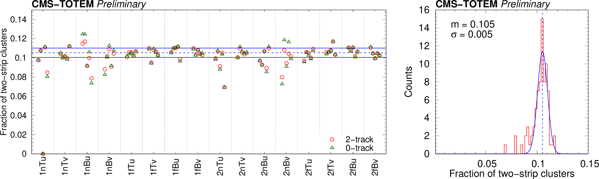
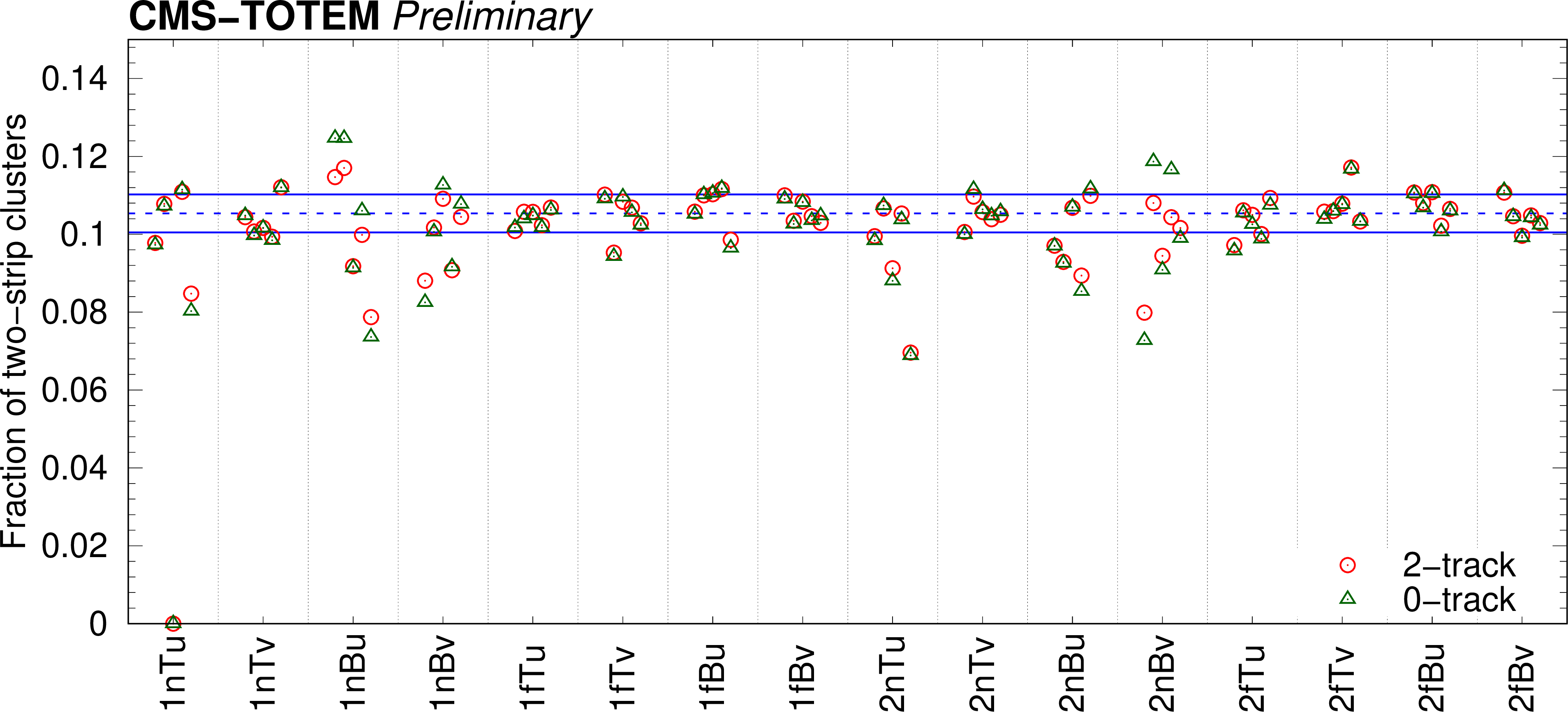
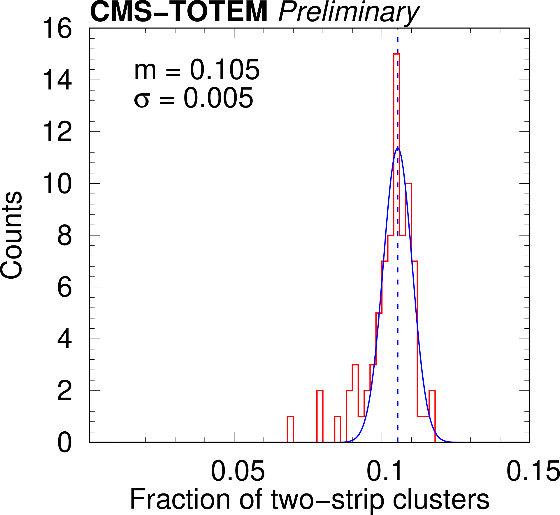
png pdf	Figure 3: Left: Fraction of two-strip clusters for each detector layer, in groups of similarly oriented layers. Right: Distribution of the fraction of two-strip clusters. Both plots indicate the results of Gaussian fits.
png pdf	Figure 3-a: Left: Fraction of two-strip clusters for each detector layer, in groups of similarly oriented layers. Right: Distribution of the fraction of two-strip clusters. Both plots indicate the results of Gaussian fits.
png pdf	Figure 3-b: Left: Fraction of two-strip clusters for each detector layer, in groups of similarly oriented layers. Right: Distribution of the fraction of two-strip clusters. Both plots indicate the results of Gaussian fits.
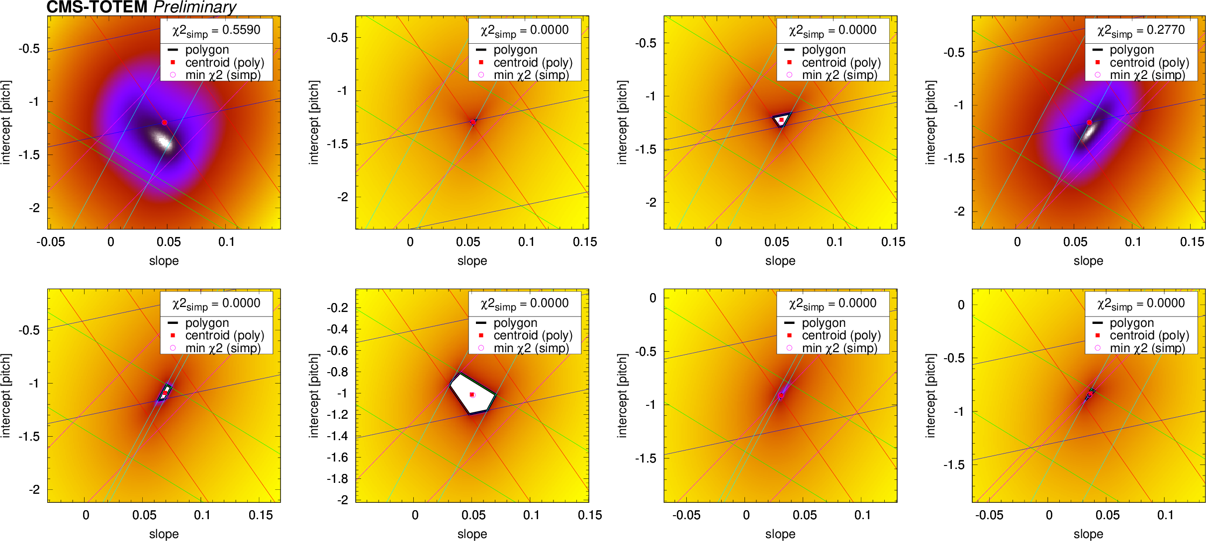
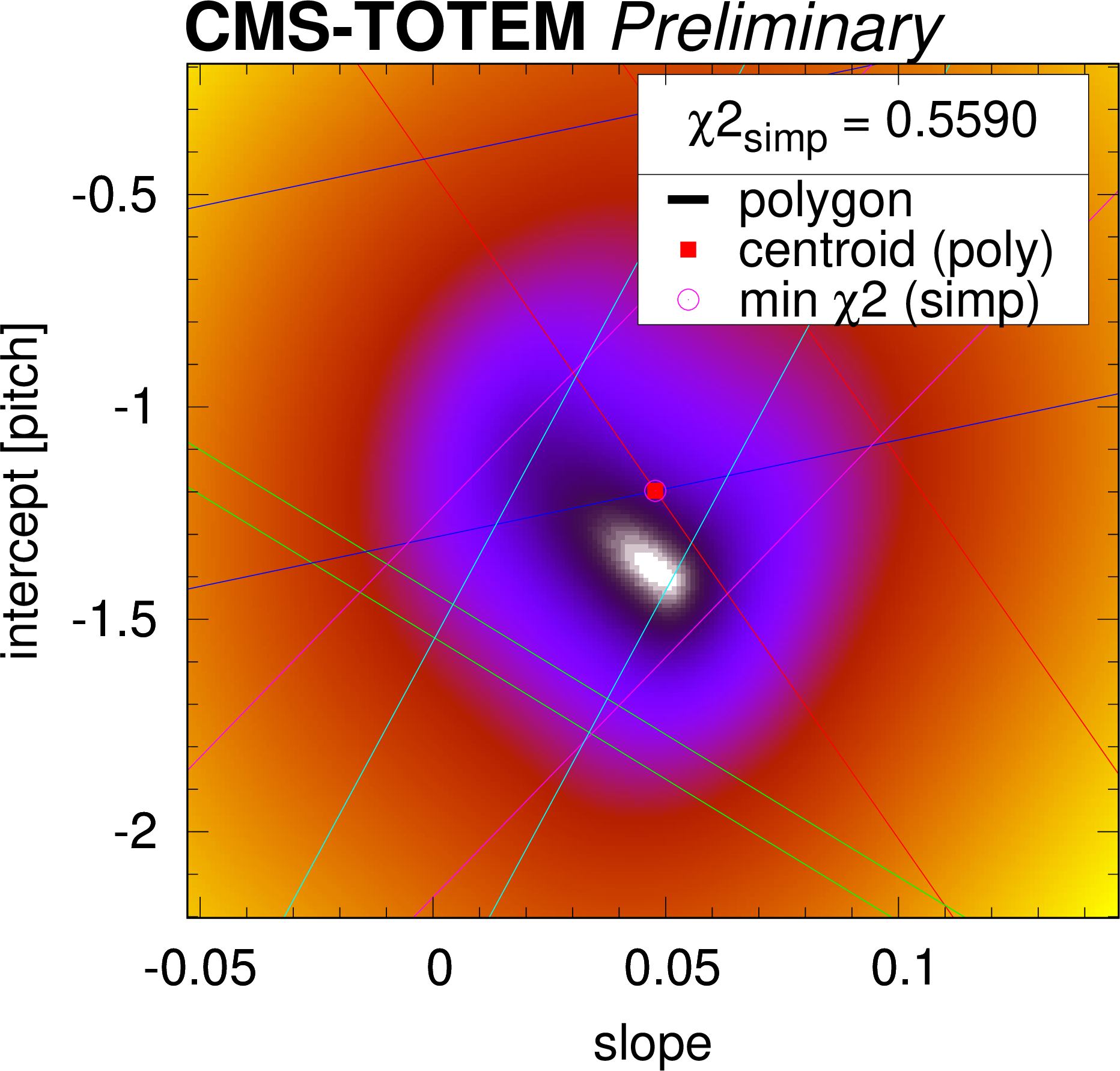
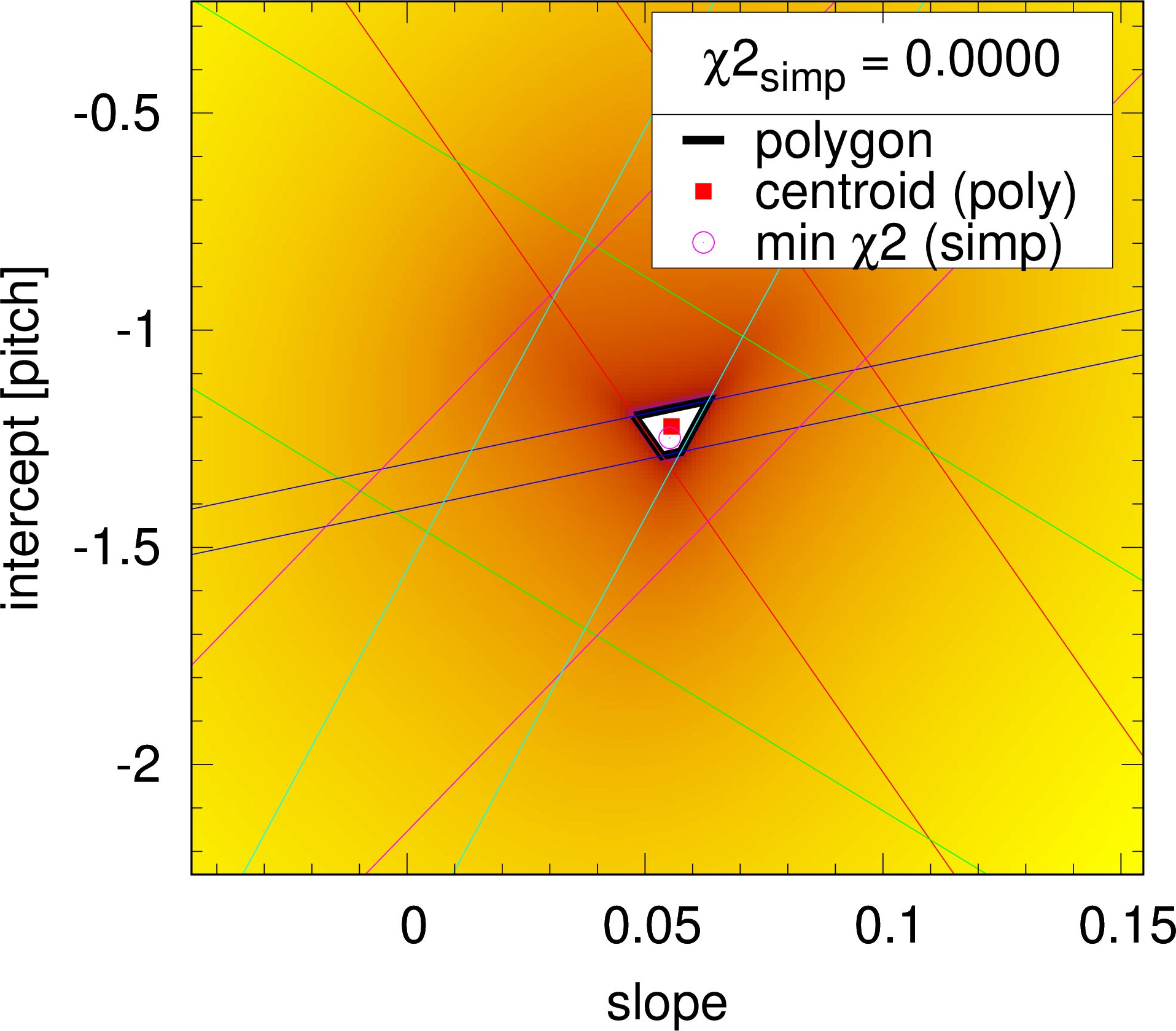
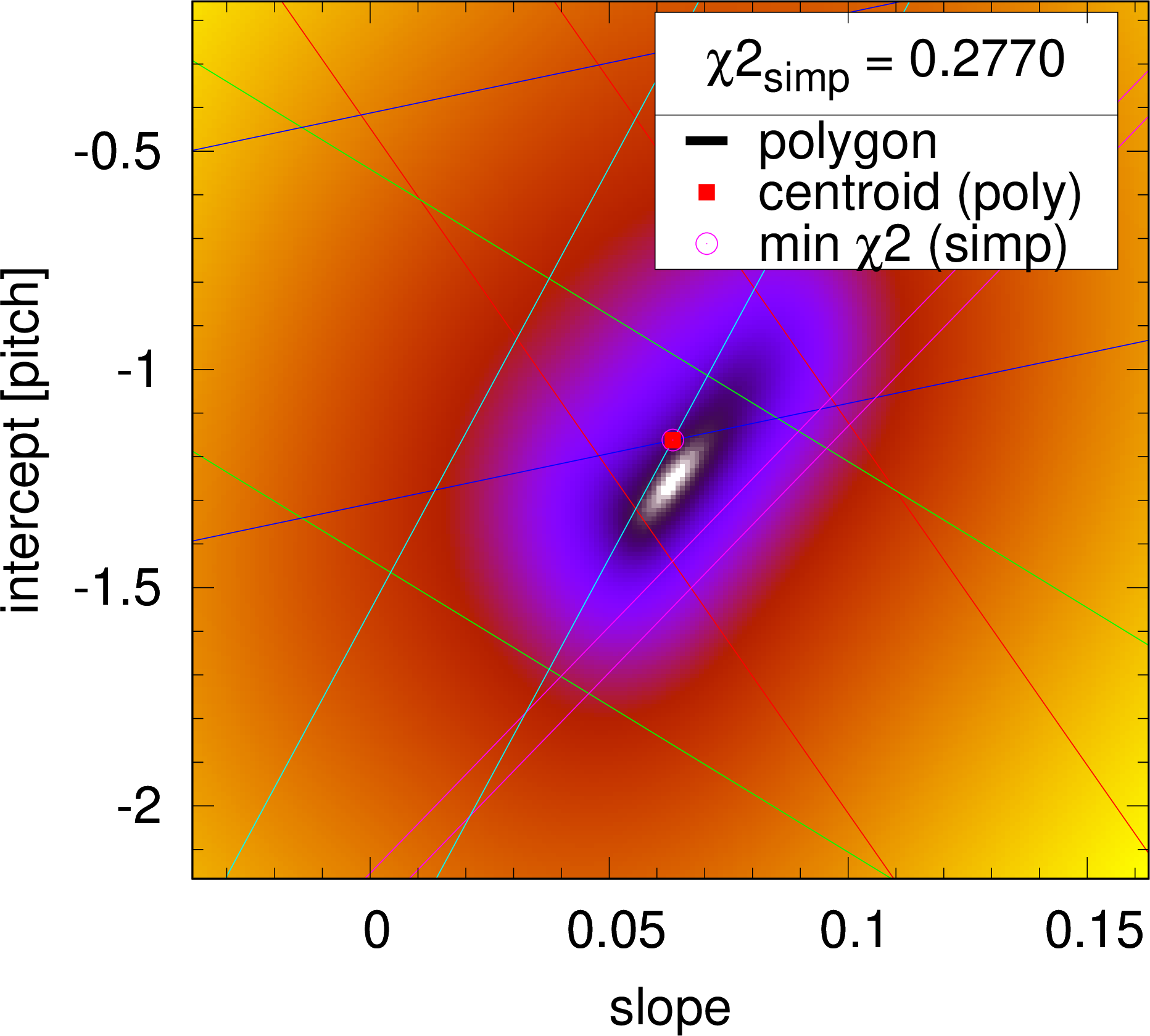
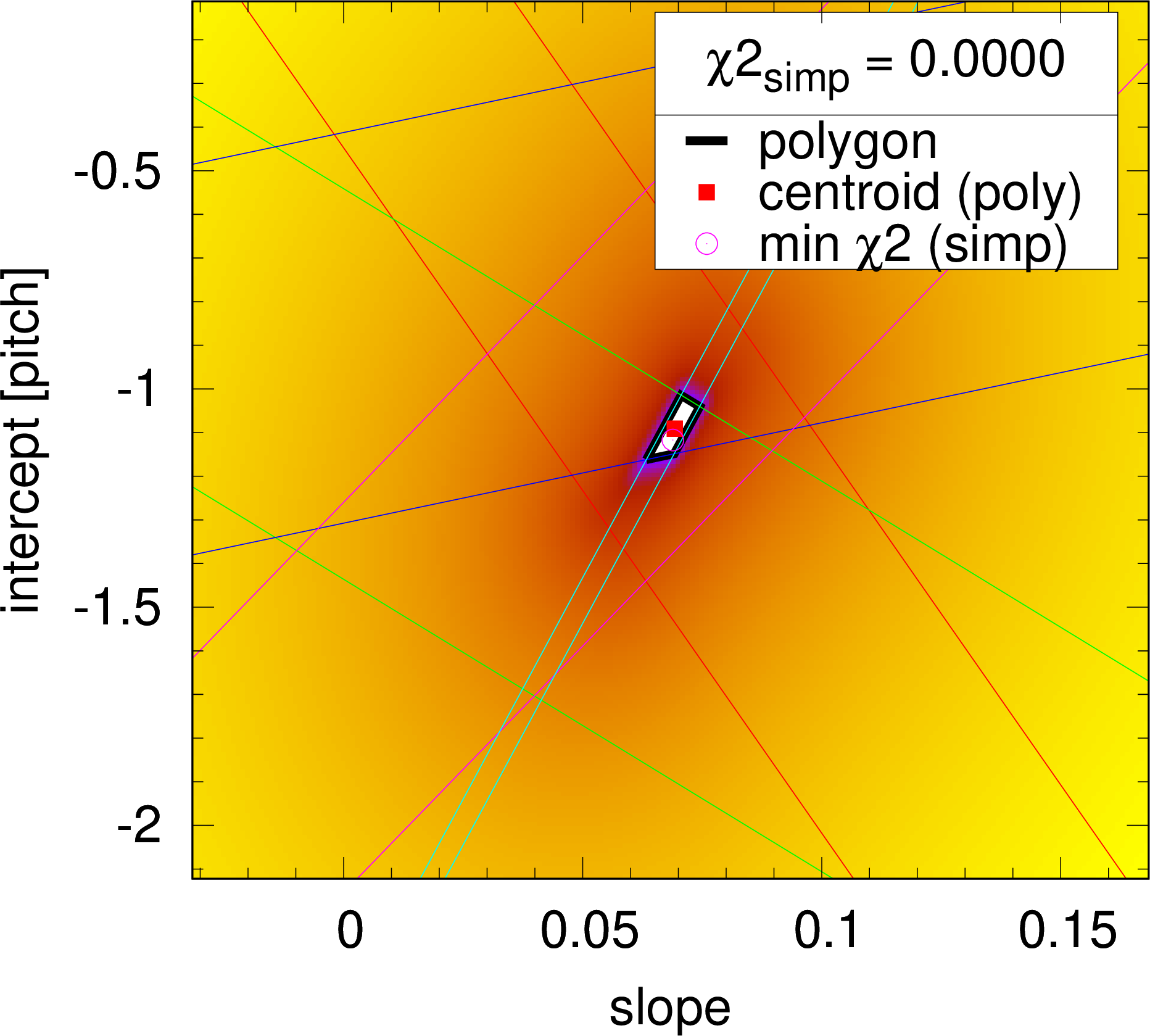
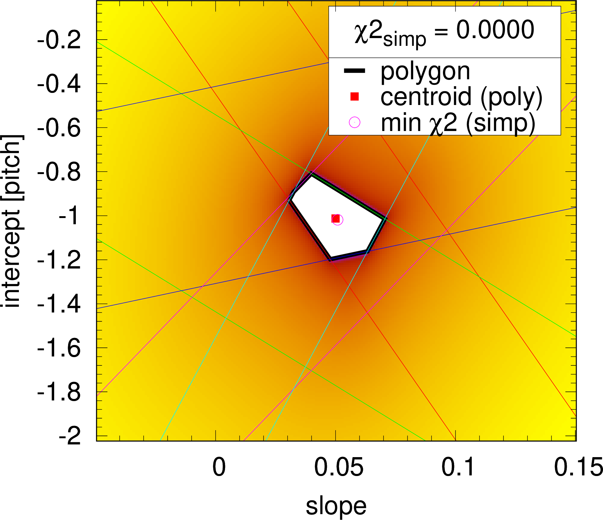
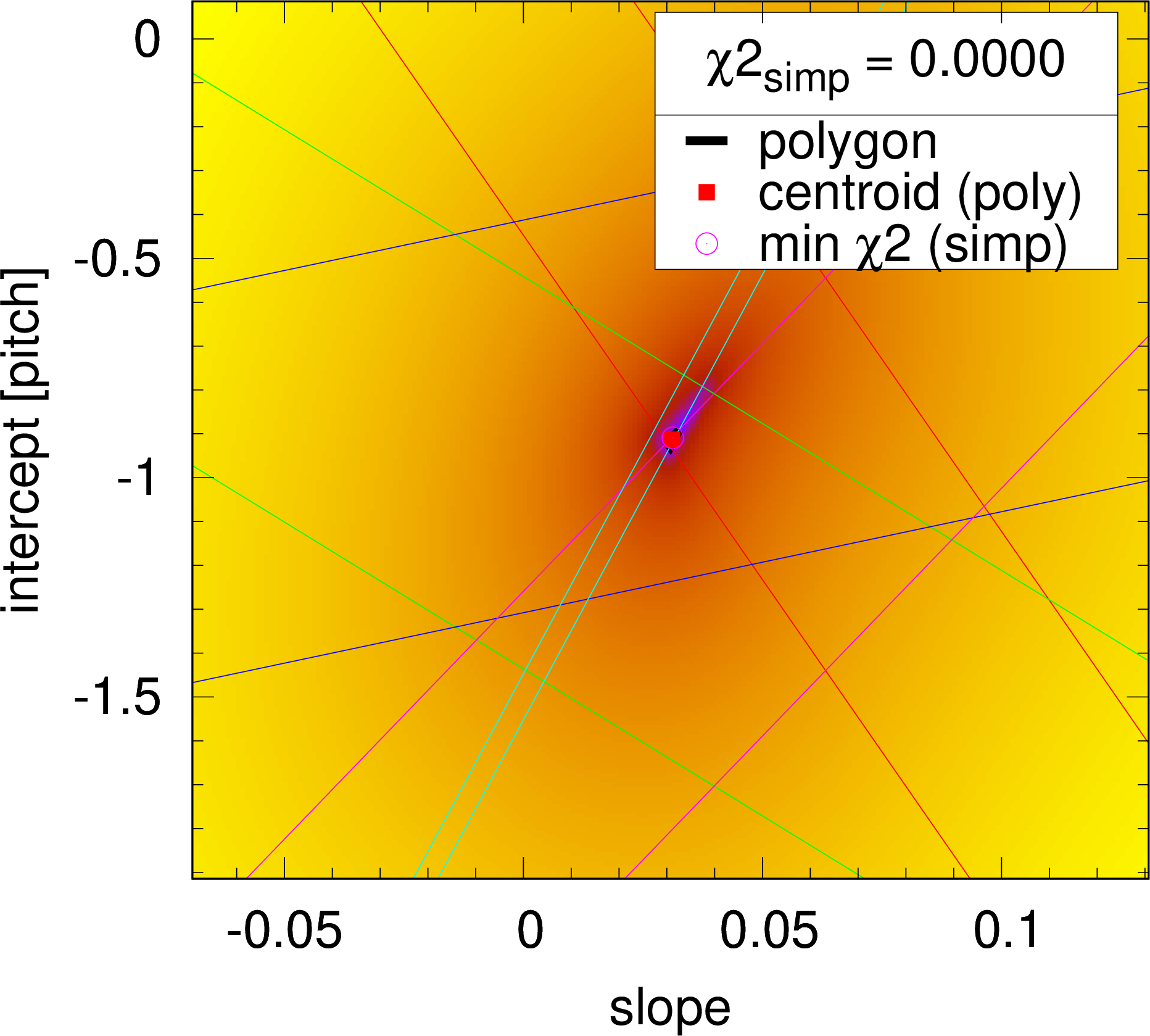
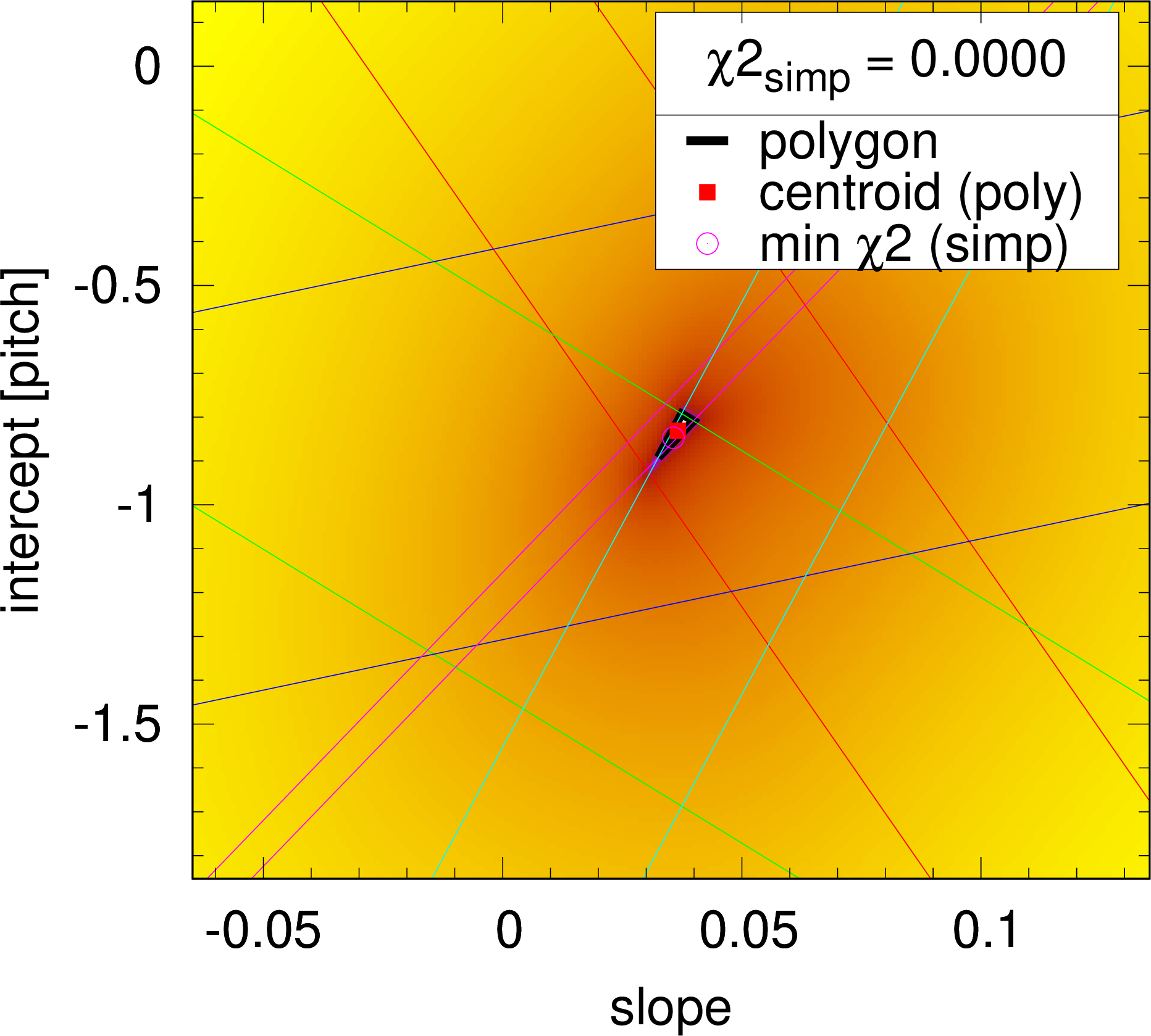
png pdf	Figure 4: Examples of tracklet fits. The gradient colour represents the value of $\chi^2$ in the intercept-slope ( $b$ - $a$ ) plane. Bands corresponding to individual detector layers are shown with differently coloured parallel straight lines. The intersection of these bands, if it exists, is shown as a white polygonal area ( $\chi^2 =$ 0) framed with thick black lines, and its centroid is marked with a red box. In each plot, the result of the simplex minimisation is indicated with a purple open circle.
png pdf	Figure 4-a: Examples of tracklet fits. The gradient colour represents the value of $\chi^2$ in the intercept-slope ( $b$ - $a$ ) plane. Bands corresponding to individual detector layers are shown with differently coloured parallel straight lines. The intersection of these bands, if it exists, is shown as a white polygonal area ( $\chi^2 =$ 0) framed with thick black lines, and its centroid is marked with a red box. In each plot, the result of the simplex minimisation is indicated with a purple open circle.
png pdf	Figure 4-b: Examples of tracklet fits. The gradient colour represents the value of $\chi^2$ in the intercept-slope ( $b$ - $a$ ) plane. Bands corresponding to individual detector layers are shown with differently coloured parallel straight lines. The intersection of these bands, if it exists, is shown as a white polygonal area ( $\chi^2 =$ 0) framed with thick black lines, and its centroid is marked with a red box. In each plot, the result of the simplex minimisation is indicated with a purple open circle.
png pdf	Figure 4-c: Examples of tracklet fits. The gradient colour represents the value of $\chi^2$ in the intercept-slope ( $b$ - $a$ ) plane. Bands corresponding to individual detector layers are shown with differently coloured parallel straight lines. The intersection of these bands, if it exists, is shown as a white polygonal area ( $\chi^2 =$ 0) framed with thick black lines, and its centroid is marked with a red box. In each plot, the result of the simplex minimisation is indicated with a purple open circle.
png pdf	Figure 4-d: Examples of tracklet fits. The gradient colour represents the value of $\chi^2$ in the intercept-slope ( $b$ - $a$ ) plane. Bands corresponding to individual detector layers are shown with differently coloured parallel straight lines. The intersection of these bands, if it exists, is shown as a white polygonal area ( $\chi^2 =$ 0) framed with thick black lines, and its centroid is marked with a red box. In each plot, the result of the simplex minimisation is indicated with a purple open circle.
png pdf	Figure 4-e: Examples of tracklet fits. The gradient colour represents the value of $\chi^2$ in the intercept-slope ( $b$ - $a$ ) plane. Bands corresponding to individual detector layers are shown with differently coloured parallel straight lines. The intersection of these bands, if it exists, is shown as a white polygonal area ( $\chi^2 =$ 0) framed with thick black lines, and its centroid is marked with a red box. In each plot, the result of the simplex minimisation is indicated with a purple open circle.
png pdf	Figure 4-f: Examples of tracklet fits. The gradient colour represents the value of $\chi^2$ in the intercept-slope ( $b$ - $a$ ) plane. Bands corresponding to individual detector layers are shown with differently coloured parallel straight lines. The intersection of these bands, if it exists, is shown as a white polygonal area ( $\chi^2 =$ 0) framed with thick black lines, and its centroid is marked with a red box. In each plot, the result of the simplex minimisation is indicated with a purple open circle.
png pdf	Figure 4-g: Examples of tracklet fits. The gradient colour represents the value of $\chi^2$ in the intercept-slope ( $b$ - $a$ ) plane. Bands corresponding to individual detector layers are shown with differently coloured parallel straight lines. The intersection of these bands, if it exists, is shown as a white polygonal area ( $\chi^2 =$ 0) framed with thick black lines, and its centroid is marked with a red box. In each plot, the result of the simplex minimisation is indicated with a purple open circle.
png pdf	Figure 4-h: Examples of tracklet fits. The gradient colour represents the value of $\chi^2$ in the intercept-slope ( $b$ - $a$ ) plane. Bands corresponding to individual detector layers are shown with differently coloured parallel straight lines. The intersection of these bands, if it exists, is shown as a white polygonal area ( $\chi^2 =$ 0) framed with thick black lines, and its centroid is marked with a red box. In each plot, the result of the simplex minimisation is indicated with a purple open circle.
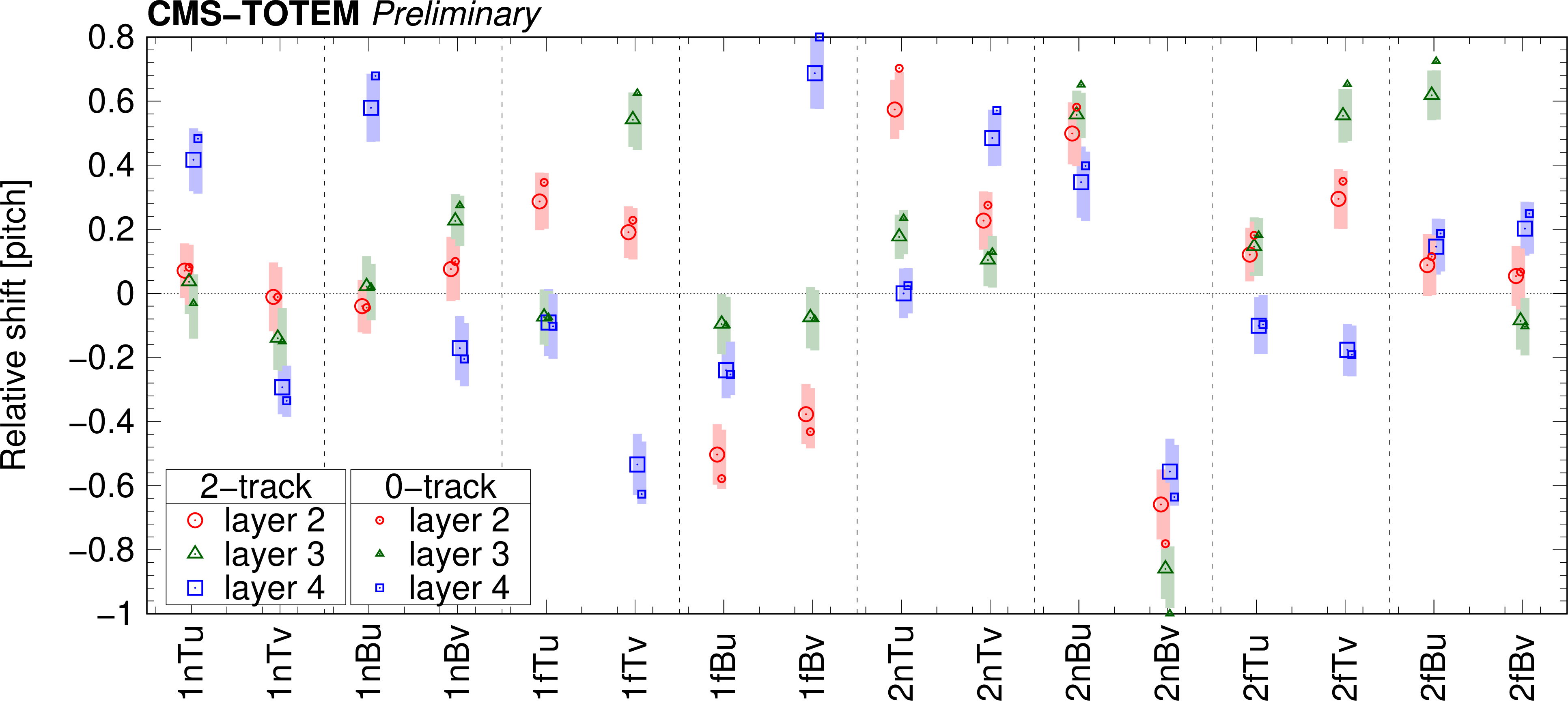
png pdf	Figure 5: Deduced alignment parameters for inner layers ( $\delta_2$ -- red circle, $\delta_3$ -- green triangle, $\delta_4$ -- blue square) in layer groups, in units of strip-width. Larger open symbols represent the 2-track data set, while the smaller ones are based on the 0-track data set. Shaded bars indicate the estimated systematic uncertainties.
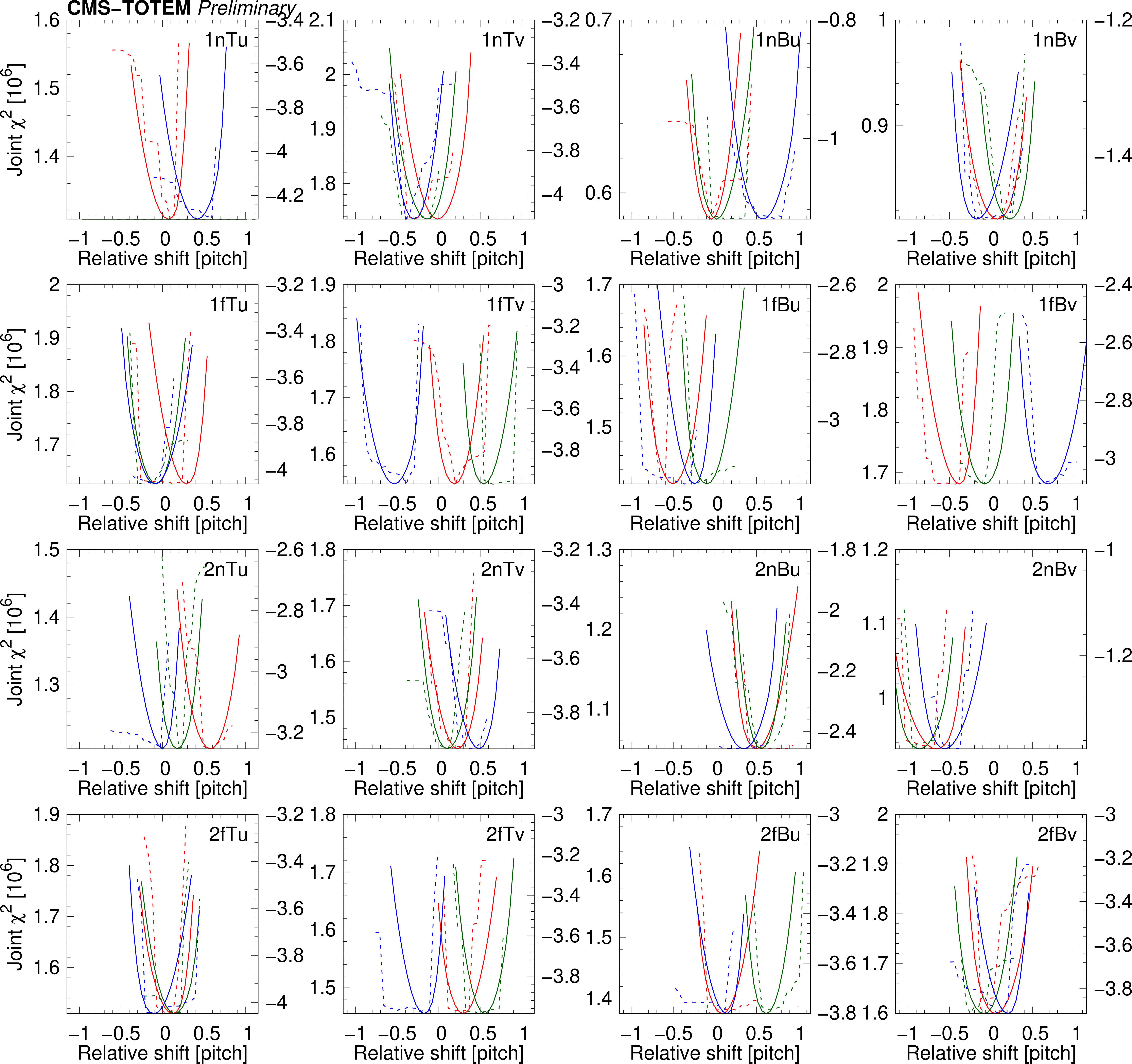
png pdf	Figure 6: One-dimensional line scans of the relative shifts ( $\delta_2$ -- red, $\delta_3$ -- green, $\delta_4$ -- blue) for the 16 layer groups around the best values found. The joint $\chi^2$ value is plotted as a function of the relative shifts of the inner layers around the found minima (solid curves, left vertical scale). Goodness-of-fit from an alternative method, counting tracks with $\chi^2 =$ 0, is also indicated (dashed lines, right vertical scale, negative of the number of such tracks in units of 10 $^7$ ). The vertical units are arbitrary.
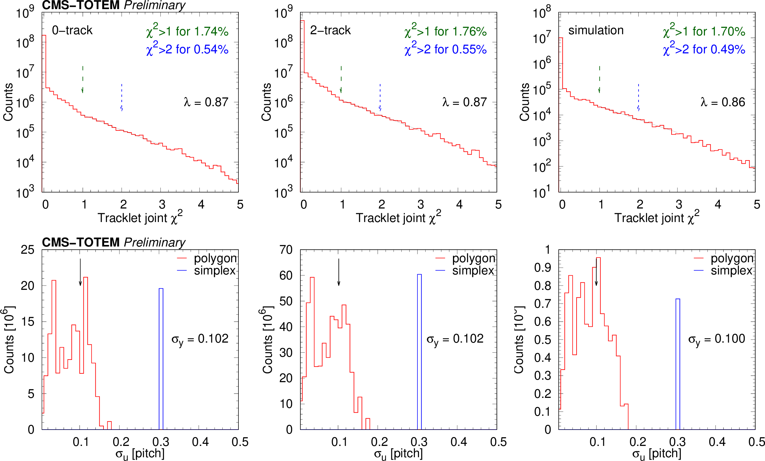
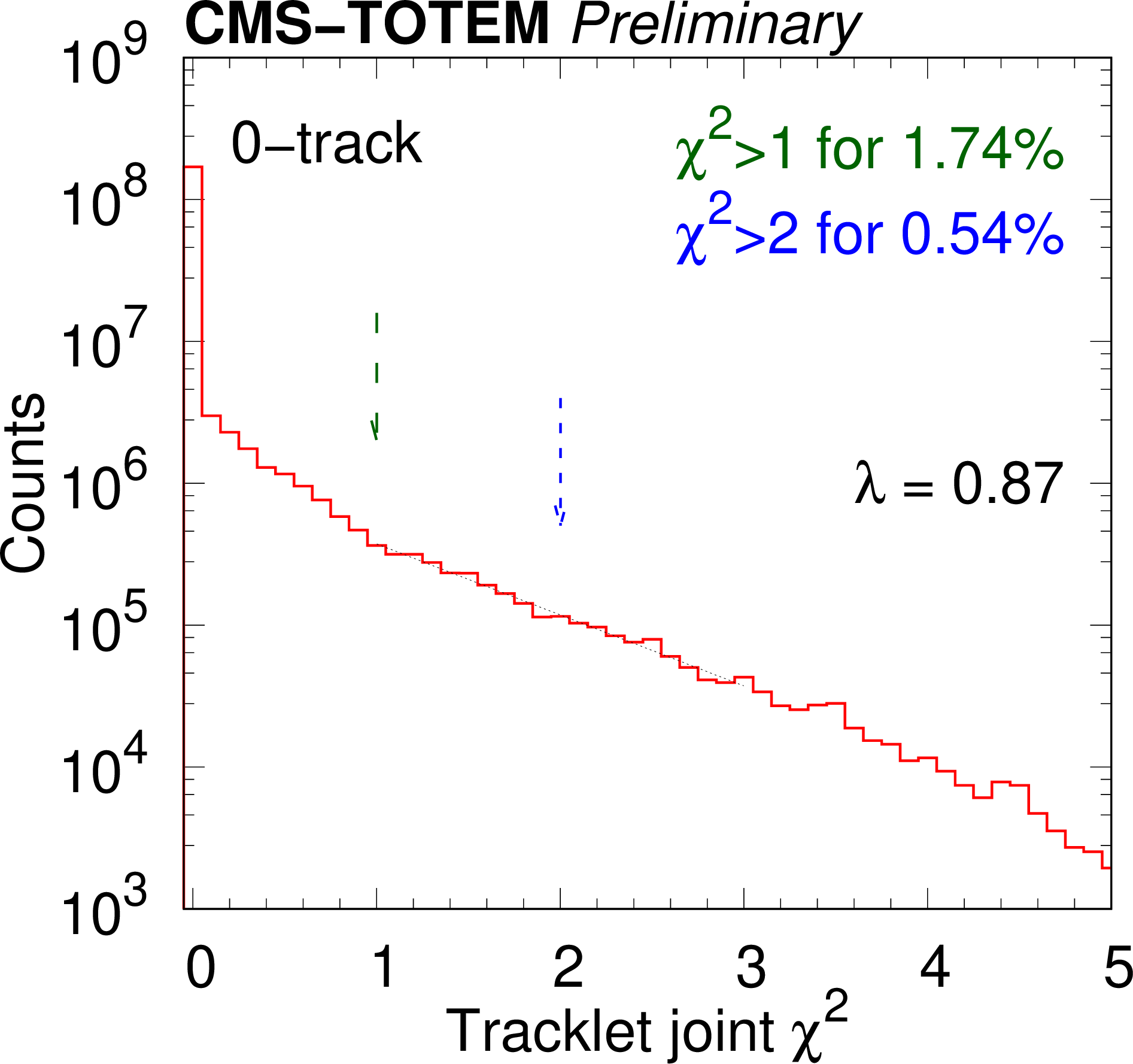
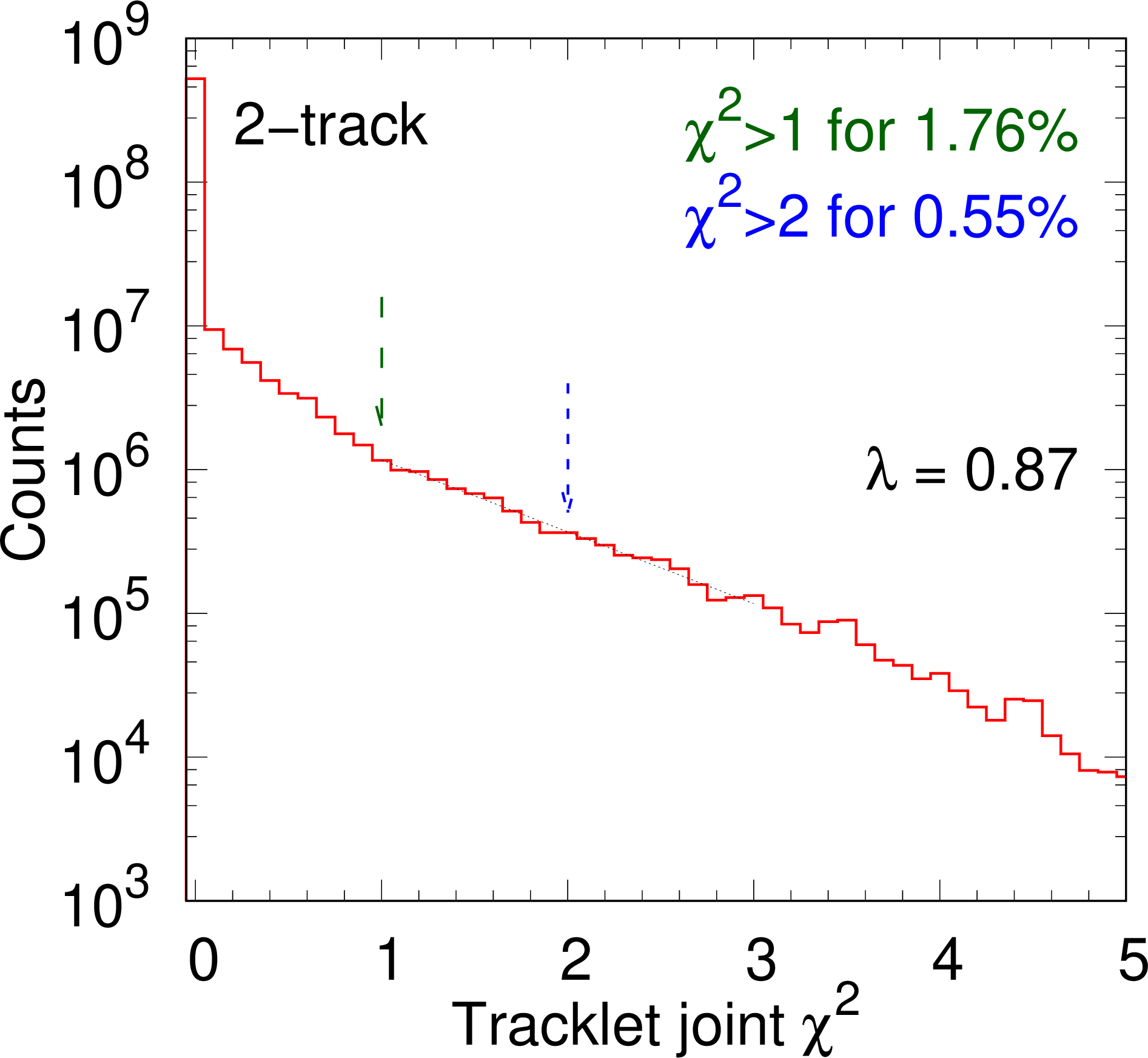
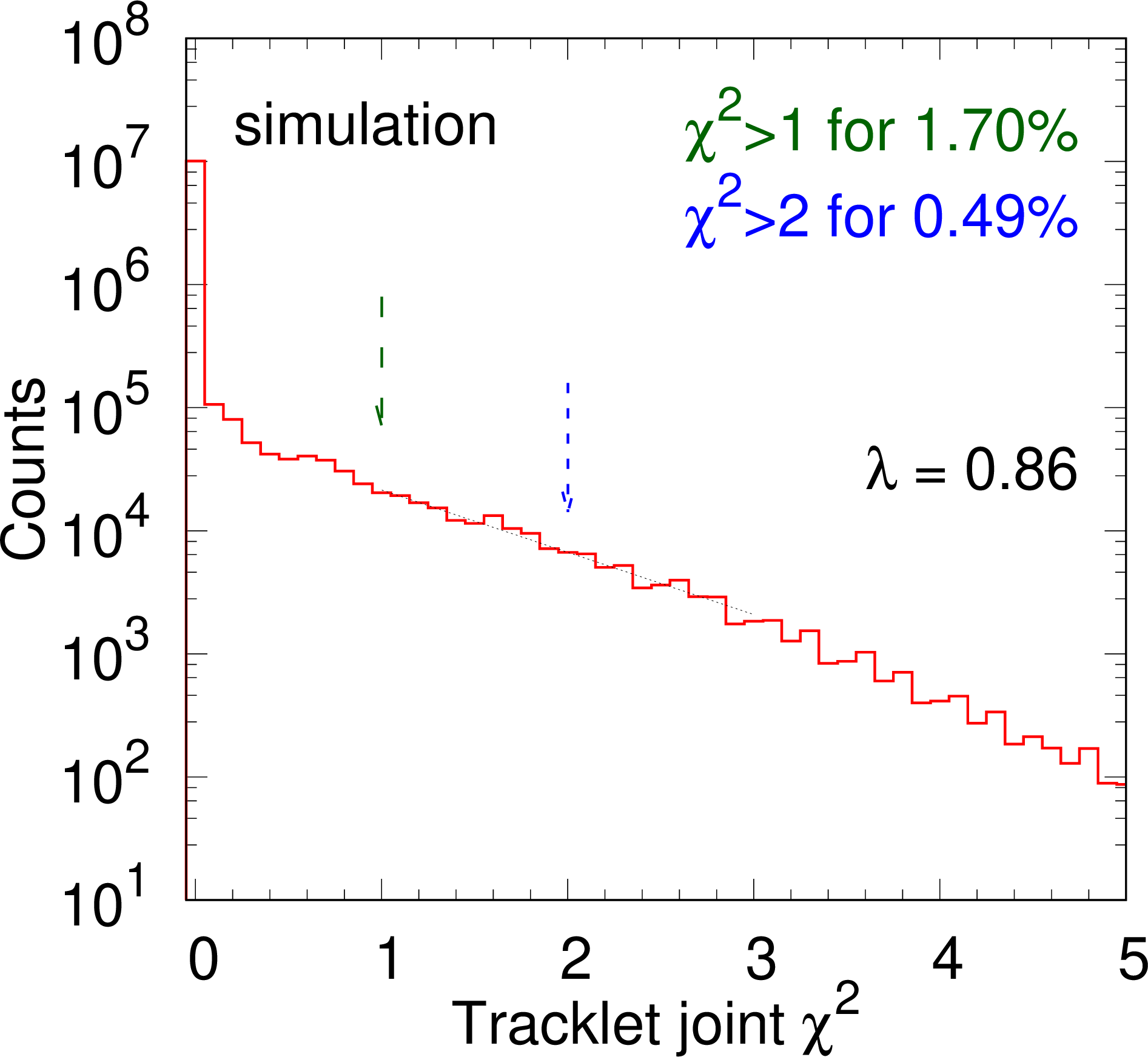
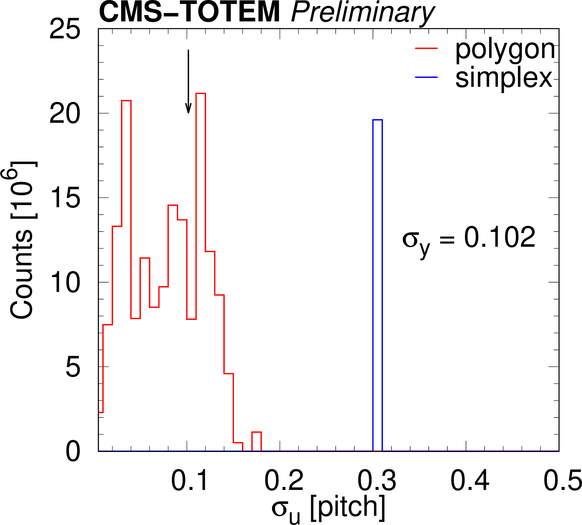
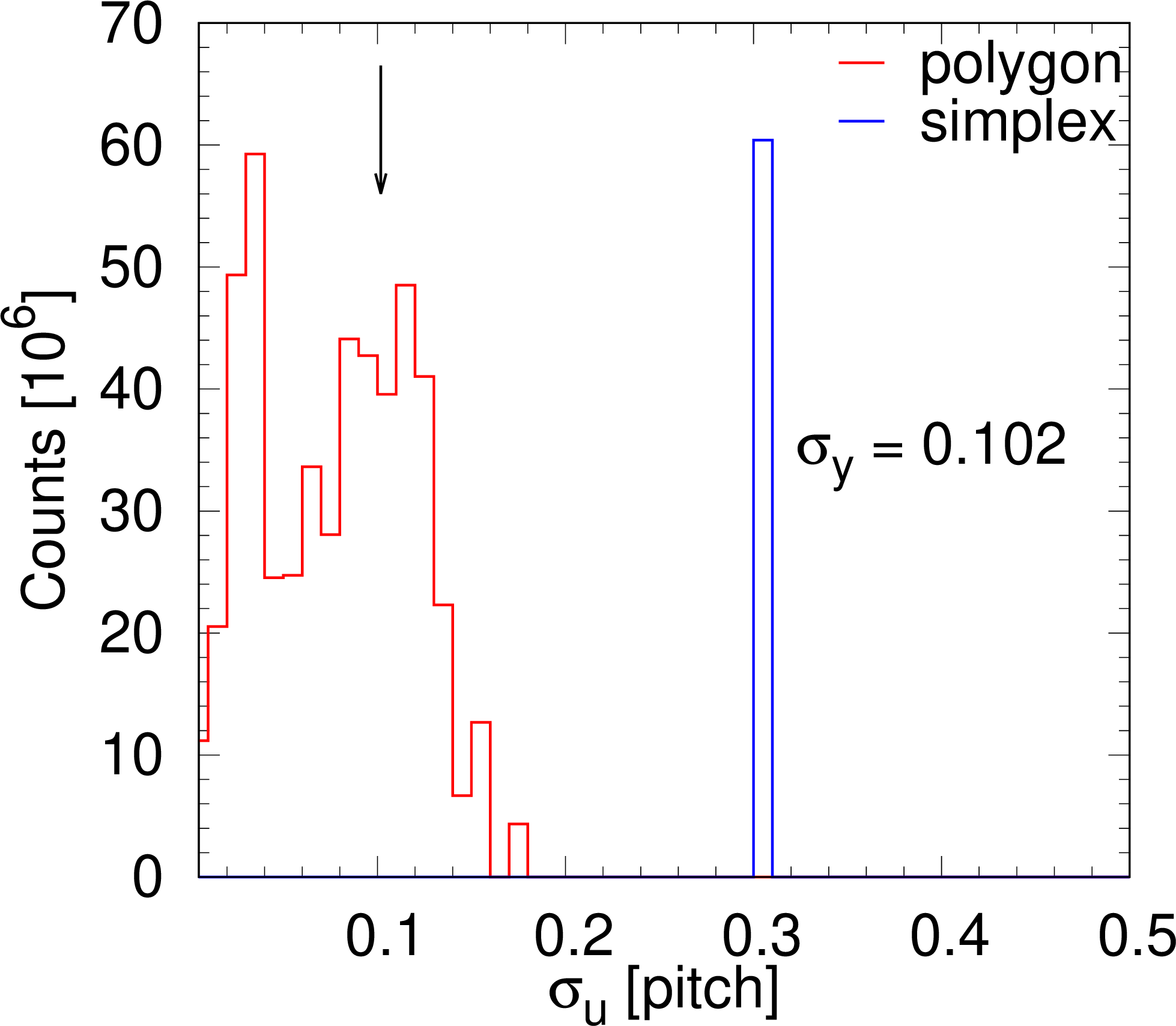
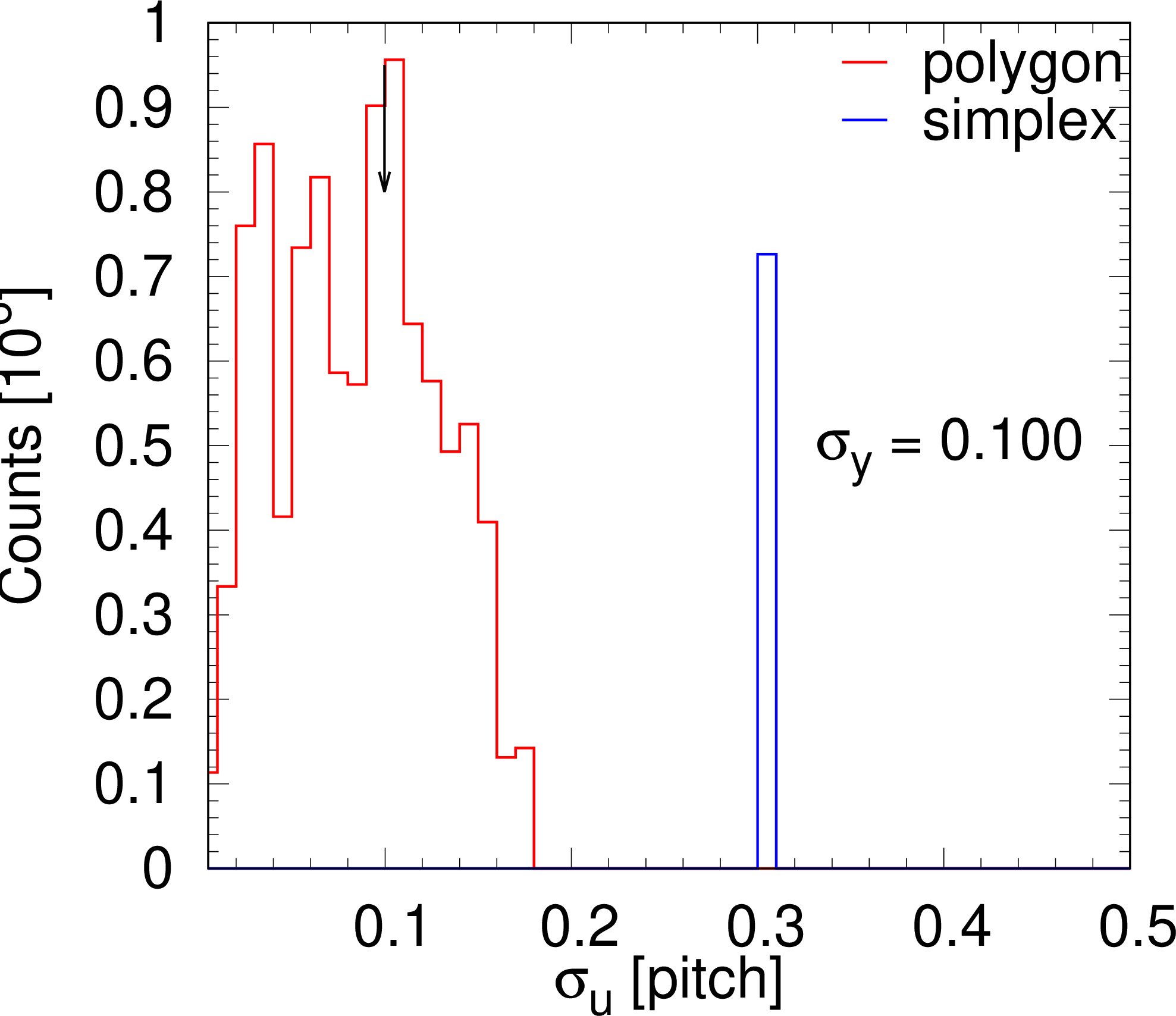
png pdf	Figure 7: Top: Distribution of the joint $\chi^2$ values for tracklets. The result for the slope $\lambda$ of an exponential fit in the range 1-3 is given. Bottom: Distribution of the standard deviation of the fitted hit location in strip-width units for the polygon method (red), and for those cases where the simplex minimisation was necessary (blue, at 0.3). The three columns correspond to the 0-track (left), 2-track (centre), and the simulated (right) data sets. The vertical arrow indicates the location of the average value.
png pdf	Figure 7-a: Top: Distribution of the joint $\chi^2$ values for tracklets. The result for the slope $\lambda$ of an exponential fit in the range 1-3 is given. Bottom: Distribution of the standard deviation of the fitted hit location in strip-width units for the polygon method (red), and for those cases where the simplex minimisation was necessary (blue, at 0.3). The three columns correspond to the 0-track (left), 2-track (centre), and the simulated (right) data sets. The vertical arrow indicates the location of the average value.
png pdf	Figure 7-b: Top: Distribution of the joint $\chi^2$ values for tracklets. The result for the slope $\lambda$ of an exponential fit in the range 1-3 is given. Bottom: Distribution of the standard deviation of the fitted hit location in strip-width units for the polygon method (red), and for those cases where the simplex minimisation was necessary (blue, at 0.3). The three columns correspond to the 0-track (left), 2-track (centre), and the simulated (right) data sets. The vertical arrow indicates the location of the average value.
png pdf	Figure 7-c: Top: Distribution of the joint $\chi^2$ values for tracklets. The result for the slope $\lambda$ of an exponential fit in the range 1-3 is given. Bottom: Distribution of the standard deviation of the fitted hit location in strip-width units for the polygon method (red), and for those cases where the simplex minimisation was necessary (blue, at 0.3). The three columns correspond to the 0-track (left), 2-track (centre), and the simulated (right) data sets. The vertical arrow indicates the location of the average value.
png pdf	Figure 7-d: Top: Distribution of the joint $\chi^2$ values for tracklets. The result for the slope $\lambda$ of an exponential fit in the range 1-3 is given. Bottom: Distribution of the standard deviation of the fitted hit location in strip-width units for the polygon method (red), and for those cases where the simplex minimisation was necessary (blue, at 0.3). The three columns correspond to the 0-track (left), 2-track (centre), and the simulated (right) data sets. The vertical arrow indicates the location of the average value.
png pdf	Figure 7-e: Top: Distribution of the joint $\chi^2$ values for tracklets. The result for the slope $\lambda$ of an exponential fit in the range 1-3 is given. Bottom: Distribution of the standard deviation of the fitted hit location in strip-width units for the polygon method (red), and for those cases where the simplex minimisation was necessary (blue, at 0.3). The three columns correspond to the 0-track (left), 2-track (centre), and the simulated (right) data sets. The vertical arrow indicates the location of the average value.
png pdf	Figure 7-f: Top: Distribution of the joint $\chi^2$ values for tracklets. The result for the slope $\lambda$ of an exponential fit in the range 1-3 is given. Bottom: Distribution of the standard deviation of the fitted hit location in strip-width units for the polygon method (red), and for those cases where the simplex minimisation was necessary (blue, at 0.3). The three columns correspond to the 0-track (left), 2-track (centre), and the simulated (right) data sets. The vertical arrow indicates the location of the average value.
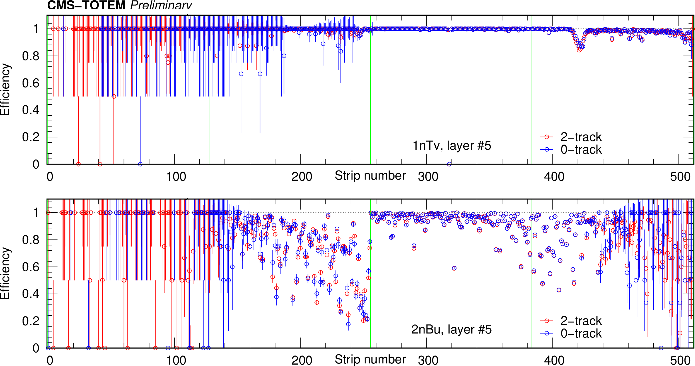
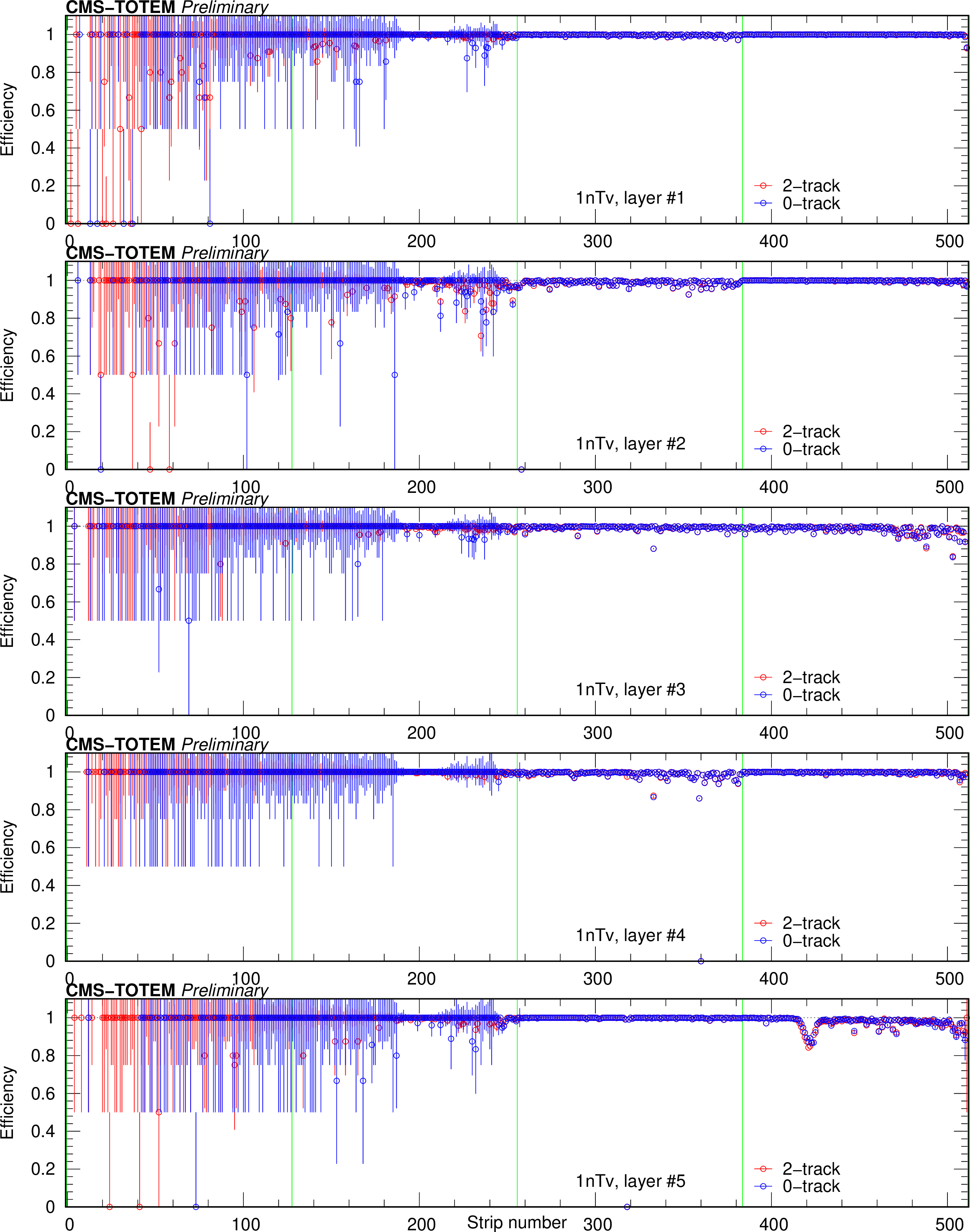
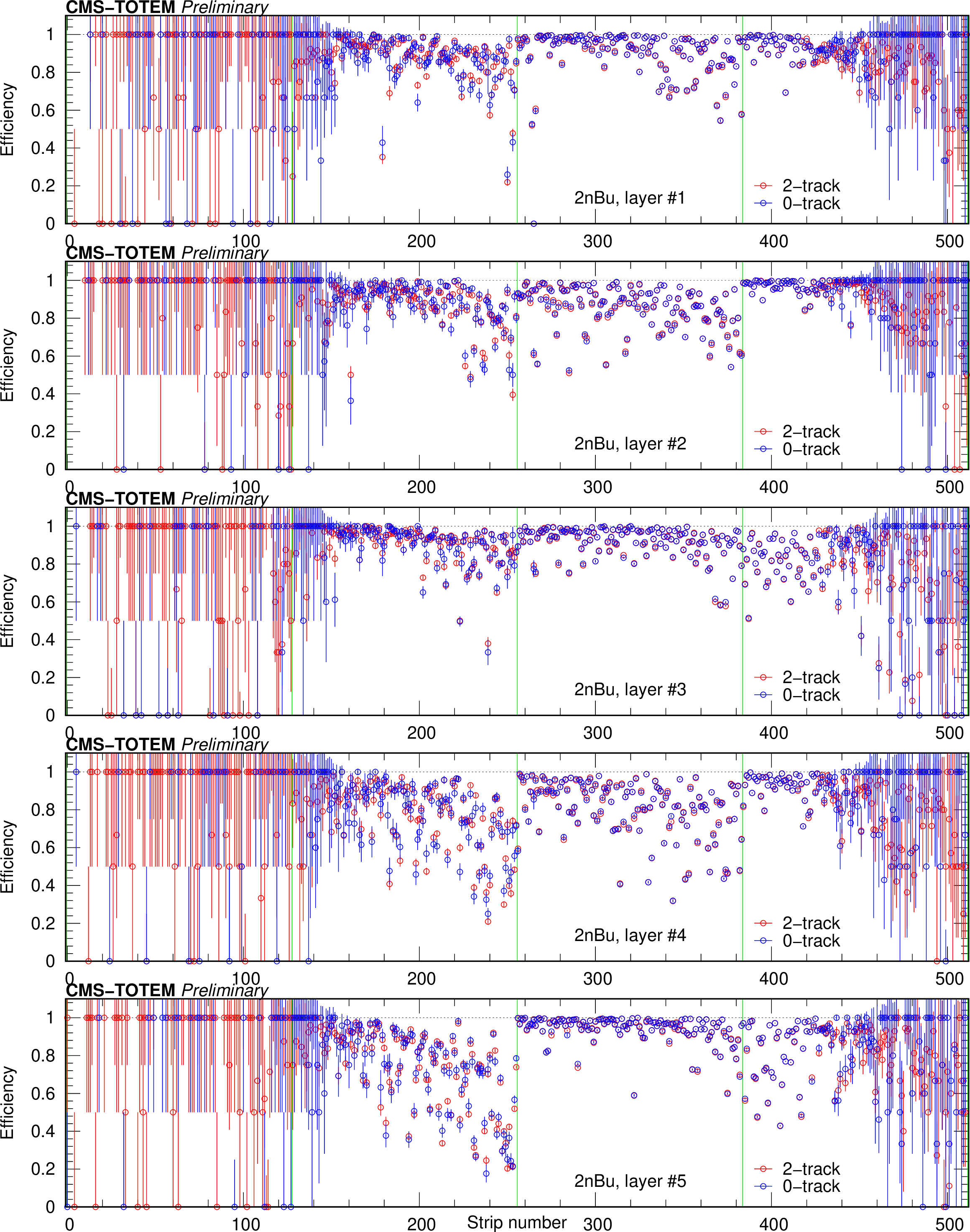
png pdf	Figure 8: Strip hit efficiency from data with a tag-and-probe method. Shown here are layer 5 in layer group 1nTv (top) and 2nBu (bottom) for a specific run. Values based on the 2-track data set (red symbols) and those from 0-track data (blue symbols) are plotted. The borders of the front-end chips are indicated with (green) vertical lines. The uncertainties are large at the left and right edges, because those regions are rarely hit.
png pdf	Figure 8-a: Strip hit efficiency from data with a tag-and-probe method. Shown here are layer 5 in layer group 1nTv (top) and 2nBu (bottom) for a specific run. Values based on the 2-track data set (red symbols) and those from 0-track data (blue symbols) are plotted. The borders of the front-end chips are indicated with (green) vertical lines. The uncertainties are large at the left and right edges, because those regions are rarely hit.
png pdf	Figure 8-b: Strip hit efficiency from data with a tag-and-probe method. Shown here are layer 5 in layer group 1nTv (top) and 2nBu (bottom) for a specific run. Values based on the 2-track data set (red symbols) and those from 0-track data (blue symbols) are plotted. The borders of the front-end chips are indicated with (green) vertical lines. The uncertainties are large at the left and right edges, because those regions are rarely hit.
png pdf	Figure 8-c: Strip hit efficiency from data with a tag-and-probe method. Shown here are layer 5 in layer group 1nTv (top) and 2nBu (bottom) for a specific run. Values based on the 2-track data set (red symbols) and those from 0-track data (blue symbols) are plotted. The borders of the front-end chips are indicated with (green) vertical lines. The uncertainties are large at the left and right edges, because those regions are rarely hit.
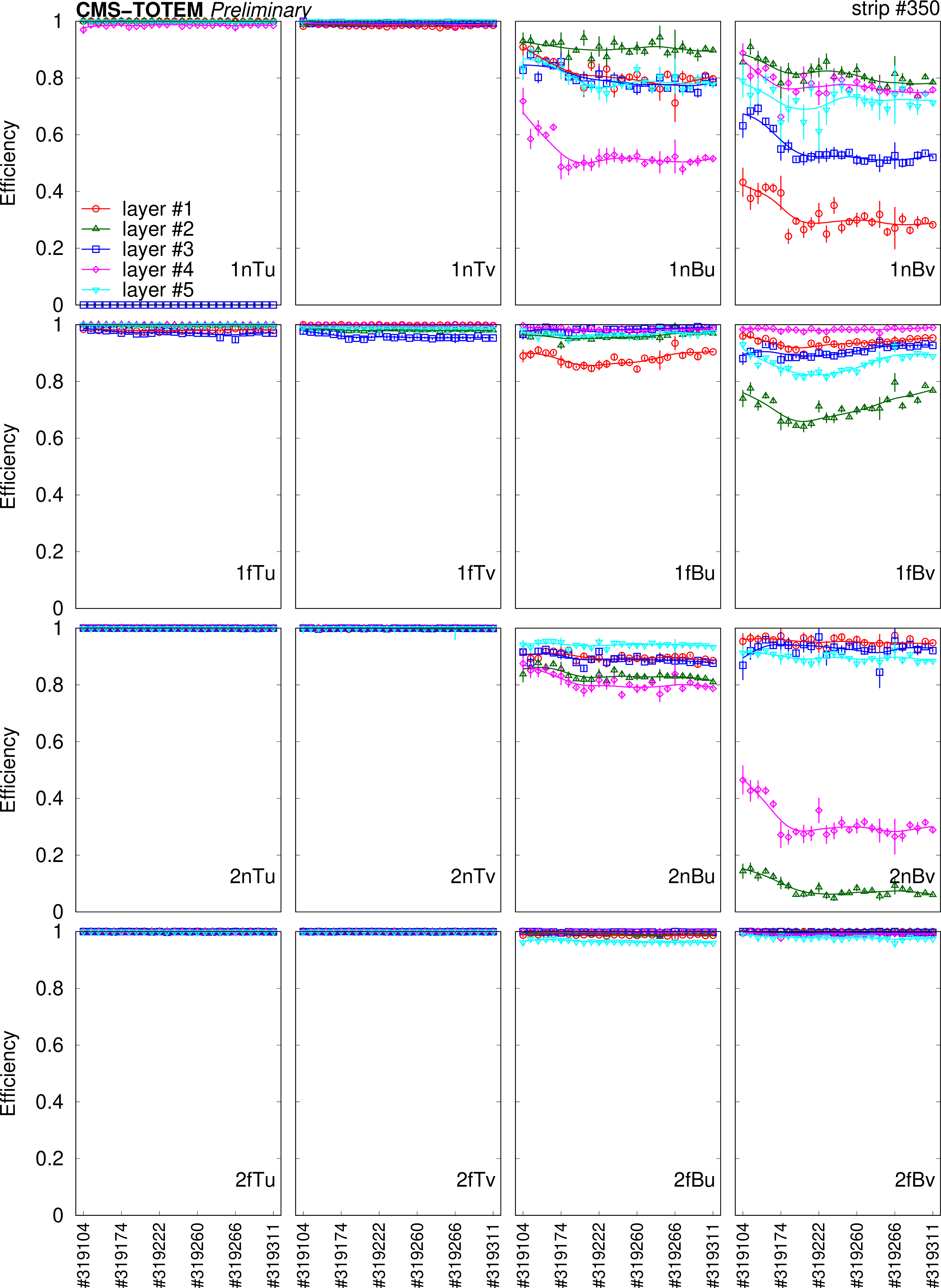
png pdf	Figure 9: Strip hit efficiencies as a function of run number for strips #350 on layers 1-5 (coloured points) in various layer groups (labels at the lower right corner). Lines are spline interpolations to guide the eye.
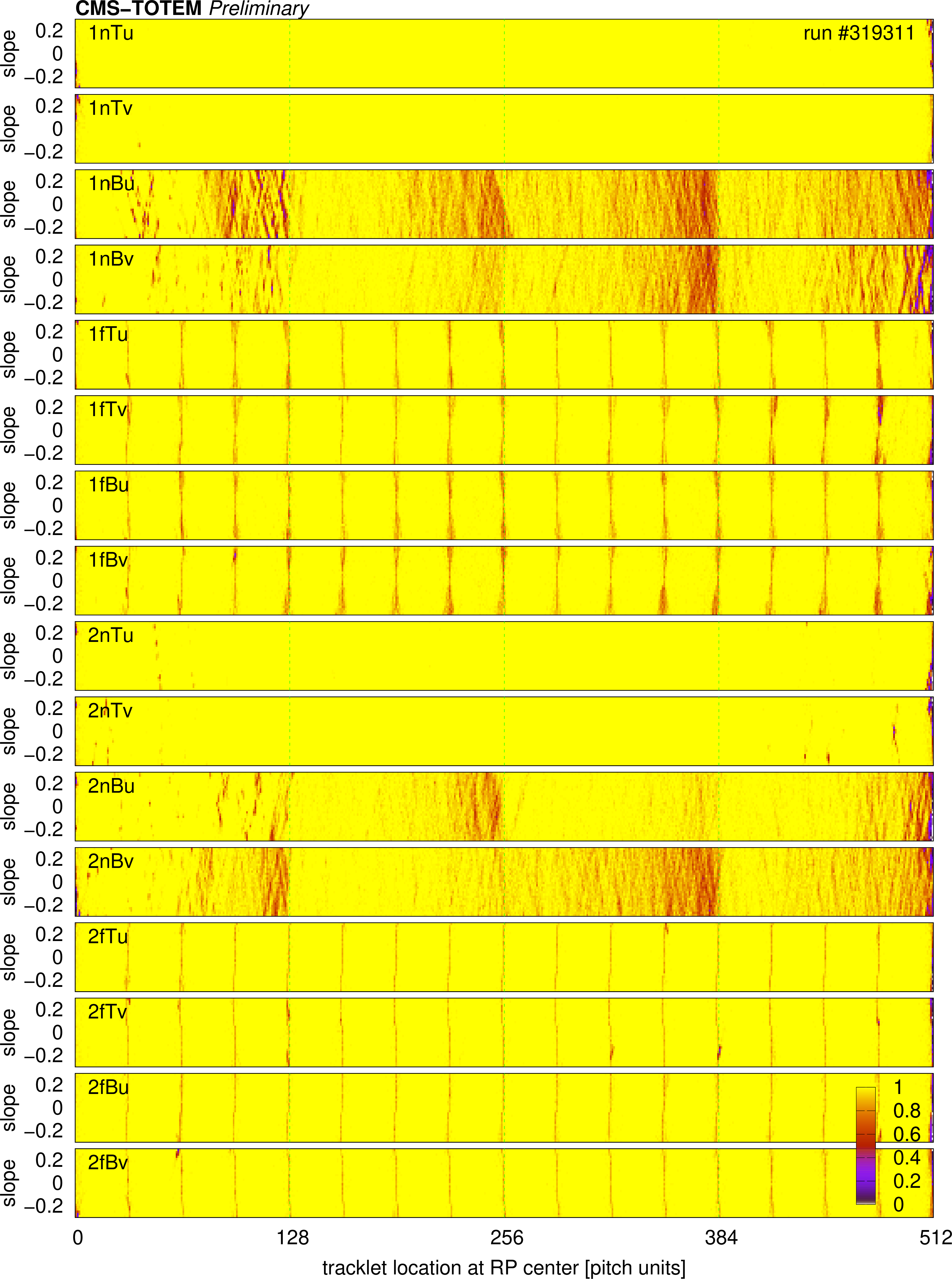
png pdf	Figure 10: Tracklet reconstruction efficiency (colour scale) as a function of tracklet location at the centre of the RP (intercept) and the track slope, for a given run, shown for each layer group separately. Yellow regions correspond to fully efficient tracklet reconstruction, whereas the red regions exhibit substantial losses with efficiencies in the range 0.4-0.6. Vertical green lines denote boundaries of the front-end chips.
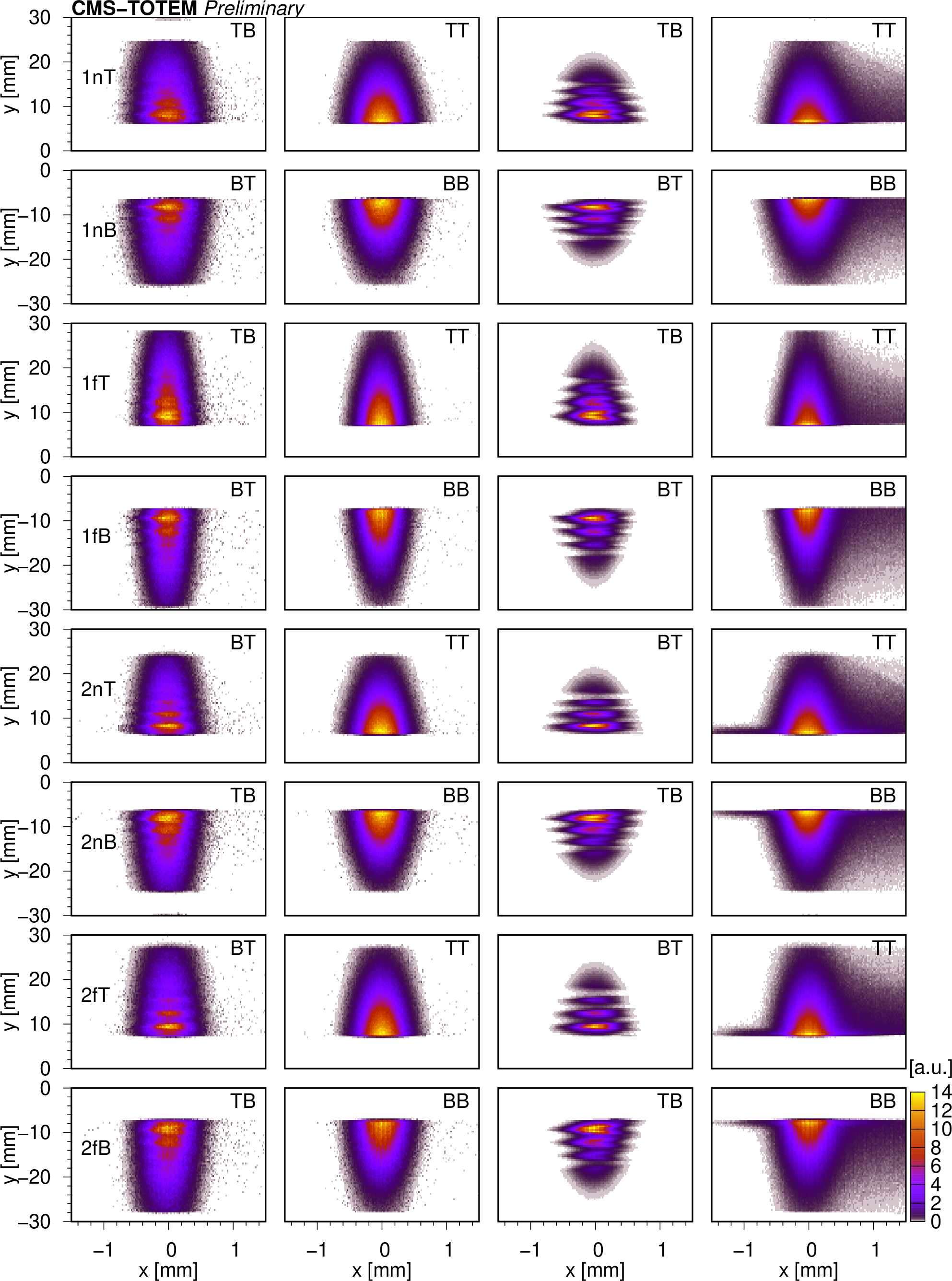
png pdf	Figure 11: Efficiency-corrected distribution of proton hit locations in the $x$ - $y$ plane at the references surfaces of the eight RPs (rows), for different trigger configurations (labels at the upper right corner). The two columns on the left side refer to the 2-track data set, whereas the two on the right side display distributions based on the 0-track data set. The wavy pattern and the halo seen in the 0-track data set is explained in the text.
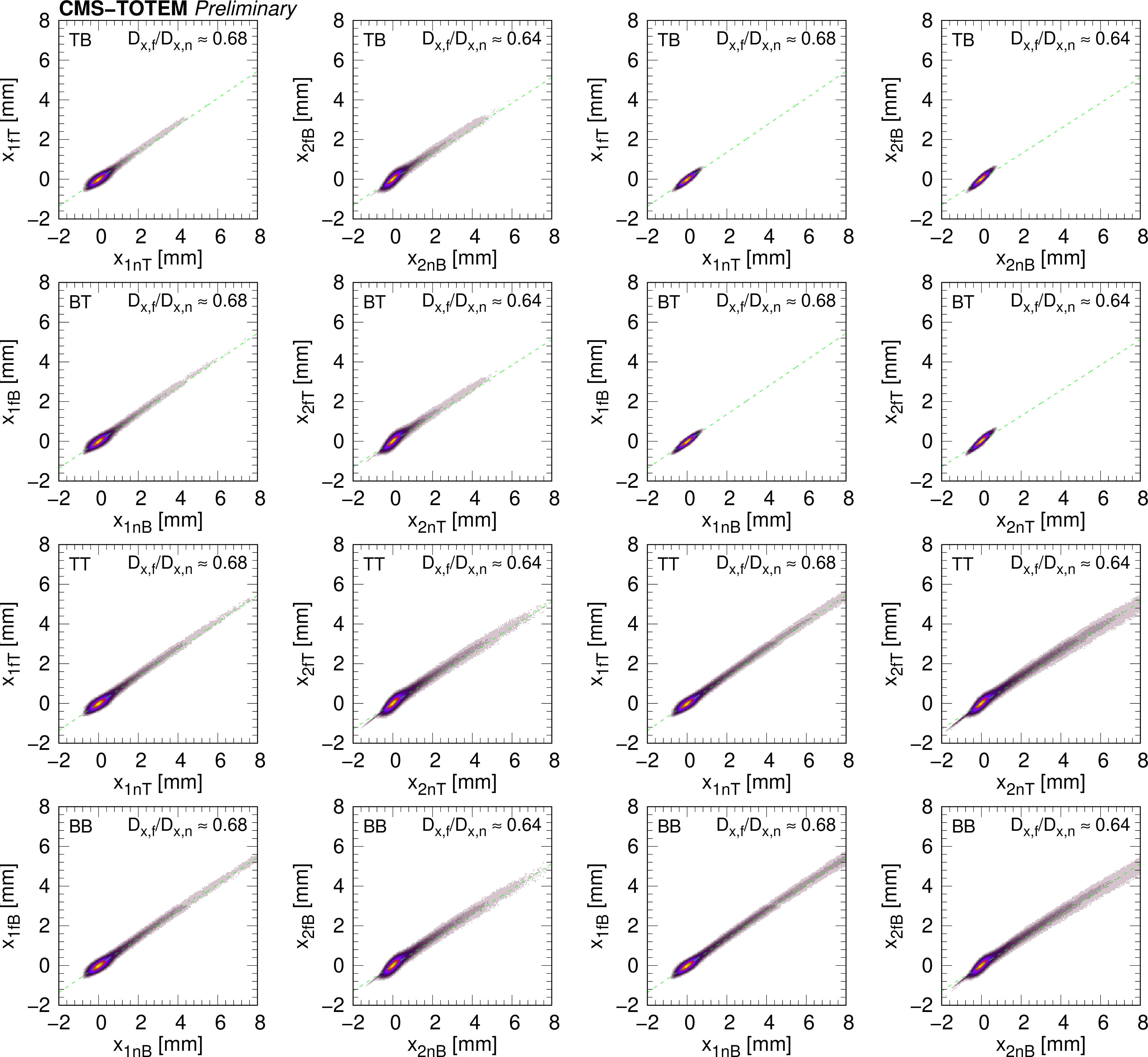
png pdf	Figure 12: Correlation of proton hit locations in $x$ direction (two-dimensional occupancy histograms) in the far and near RPs, shown for various trigger configurations (TB, BT, TT, and BB, in rows). The two columns on the left side refer to the 2-track data set, while the two on the right side display distributions based on the 0-track data set. A straight line corresponding to the expectation $x_f = x_n \cdot D_{x,f}/D_{x,n}$ is also plotted where $D_{x,f}/D_{x,n} \approx$ 0.68 for Arm 1, and $\approx$ 0.64 for Arm 2. The plots are produced with the final detector alignment.
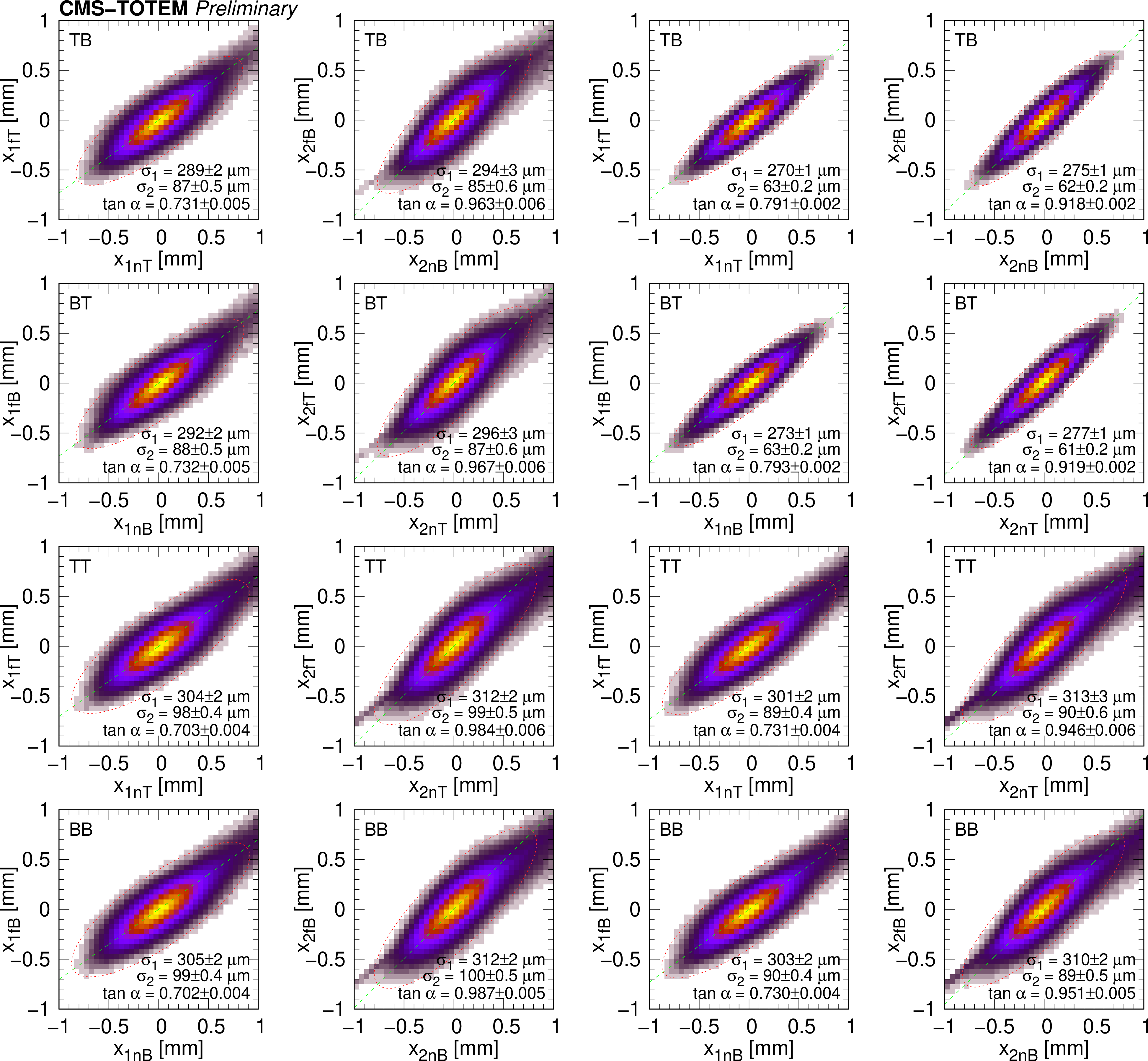
png pdf	Figure 13: Correlation of proton hit locations in the $x$ direction (two-dimensional occupancy histograms) in the far and near RPs, shown for various trigger configurations (TB, BT, TT, and BB, in rows), with a restricted scale. Parameters (standard deviations in major and minor axis directions $\sigma_1$ and $\sigma_2$ , and the rotation angle $\alpha$ ) of the fitted ellipses are displayed in the plots. The two columns on the left side refer to the 2-track data set, whereas the two on the right side display distributions based on the 0-track data set. The plots are produced with the final detector alignment.
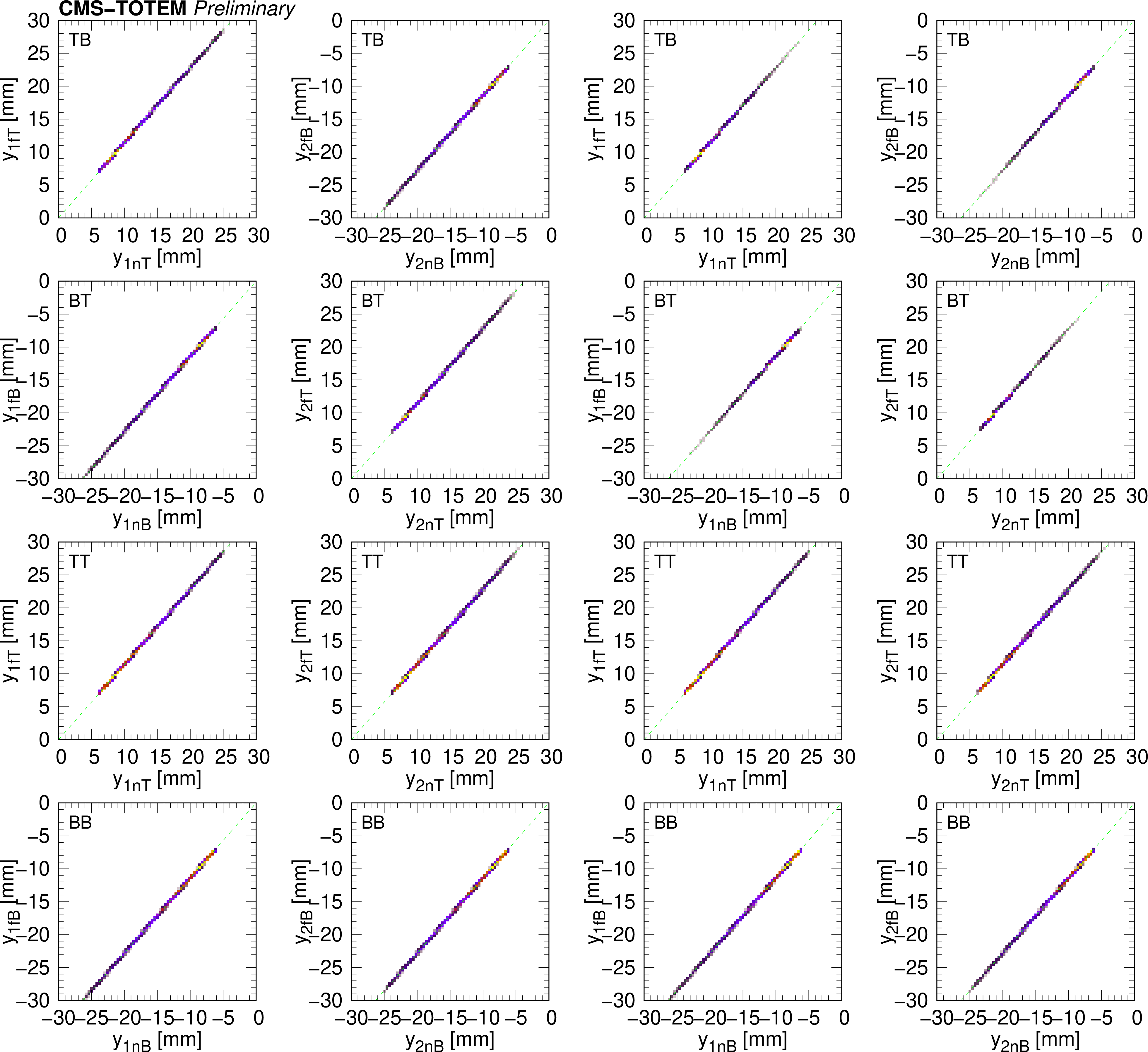
png pdf	Figure 14: Correlation of proton hit locations in the $y$ direction (two-dimensional occupancy histograms) in the far and near RPs, shown for various trigger configurations (TB, BT, TT, and BB, in rows). The two columns on the left side refer to the 2-track data set, whereas the two on the right side display distributions based on the 0-track data set. A straight line corresponding to the expectation $y_f = y_n \cdot L_{y,f}/L_{y,n}$ is also plotted, where $L_{y,f}/L_{y,n} \approx$ 1.14. The plots are produced with the final detector alignment. The apparent piecewise linear segments are simply the consequence of the binning.
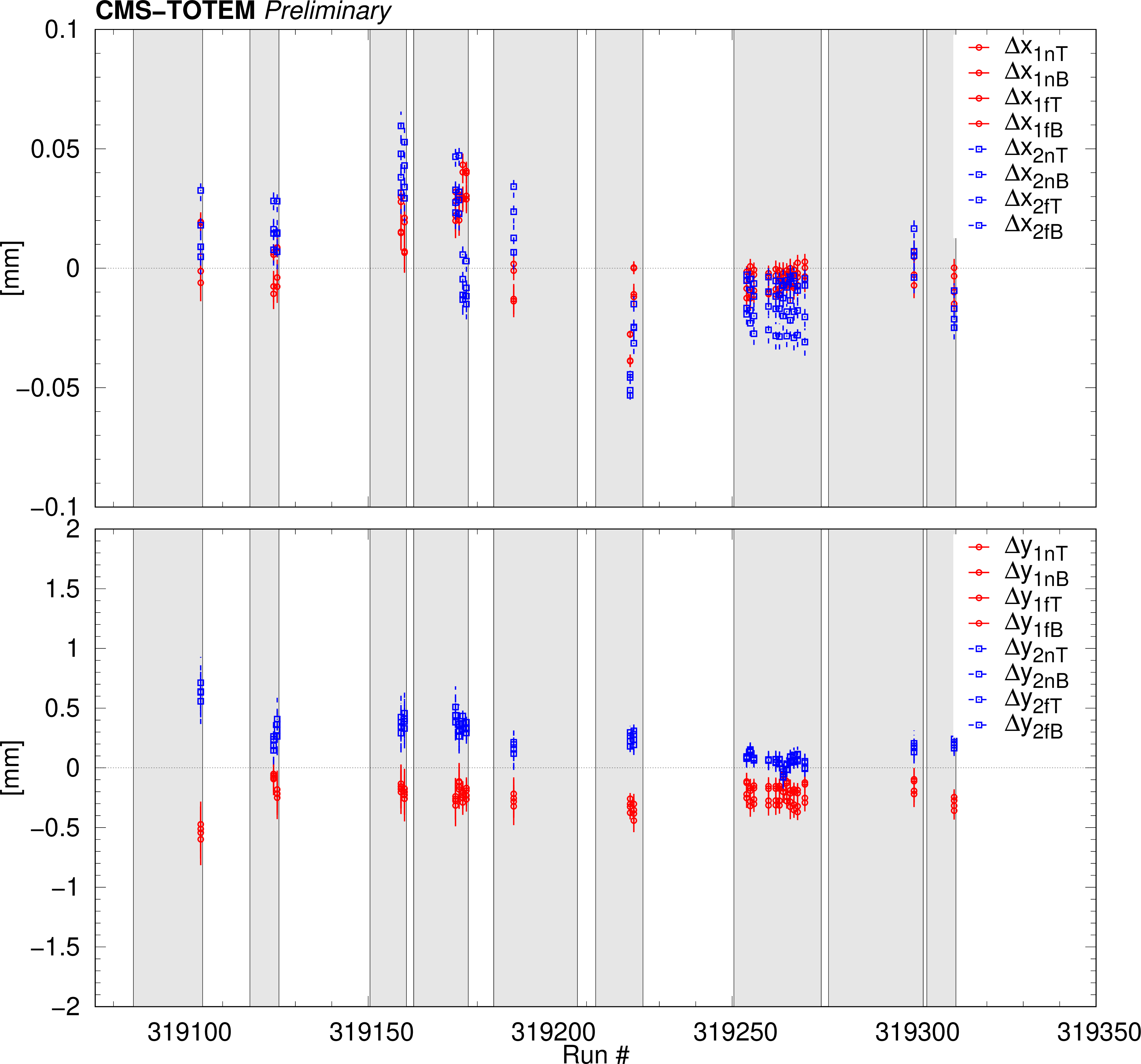
png pdf	Figure 15: Deduced displacements of RPs in the $x$ (top) and $y$ (bottom) directions as a function of run number. LHC fills are indicated by grey areas.
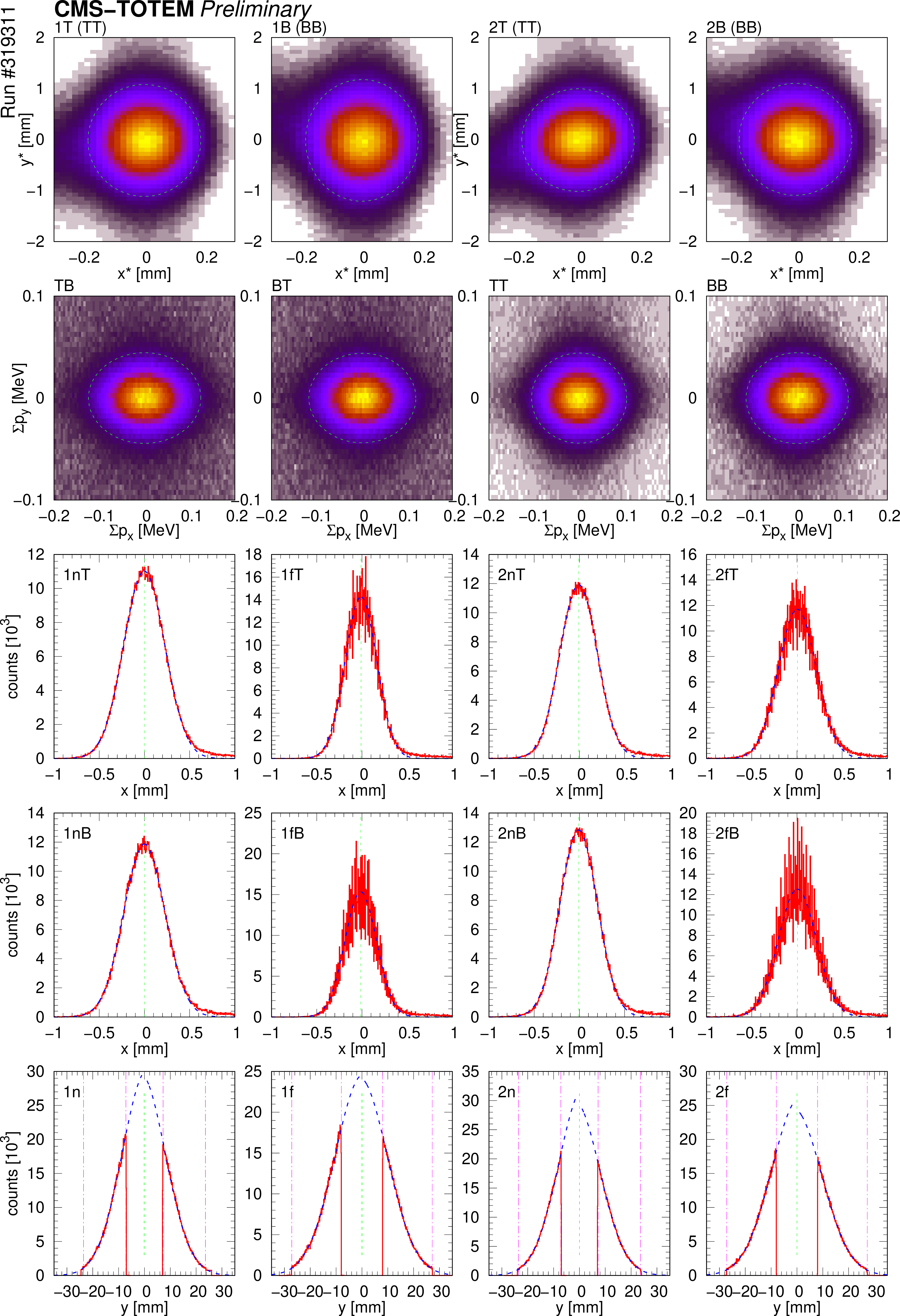
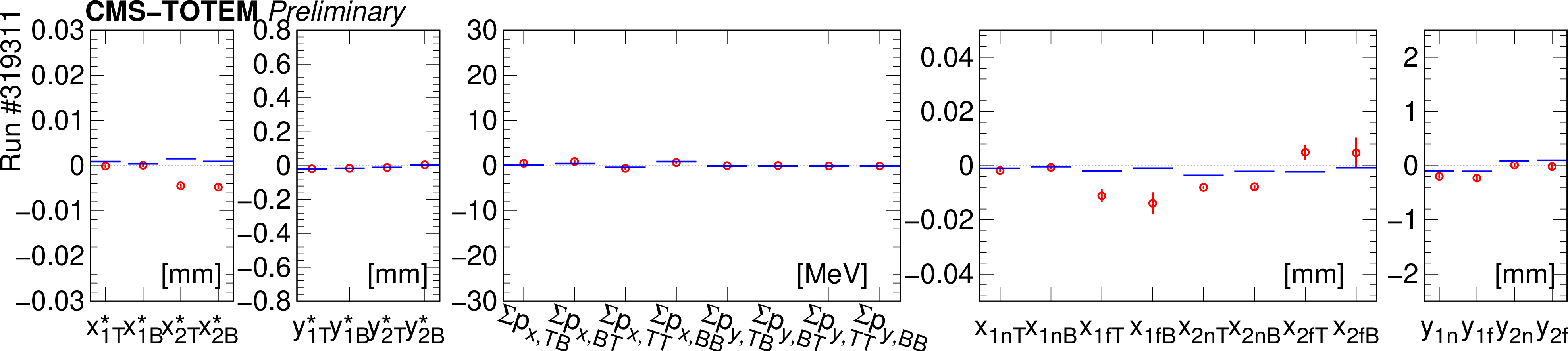
png pdf	Figure 16: Cross-check of the full alignment, shown here for run #319311. From top to bottom: Distribution of the IP $(x^,y^)$ for RP arm configurations 1T, 1B, 2T, and 2B. Distribution of the four-particle momentum sum $(\sum p_x,\sum p_y)$ for the RP trigger configurations TB, BT, TT, and BB. In both cases the 2D Gaussian fits are indicated (at 2 $\sigma$ ) with green dotted ellipses. Distribution of local hits in the RPs in the $x$ (single Gaussian) and $y$ directions (separate Gaussians). Dashed blue curves represent the Gaussian fits, vertical green dashed lines indicate the deduced relative shifts, vertical magenta dash-dotted lines on $y$ plots show fit ranges.
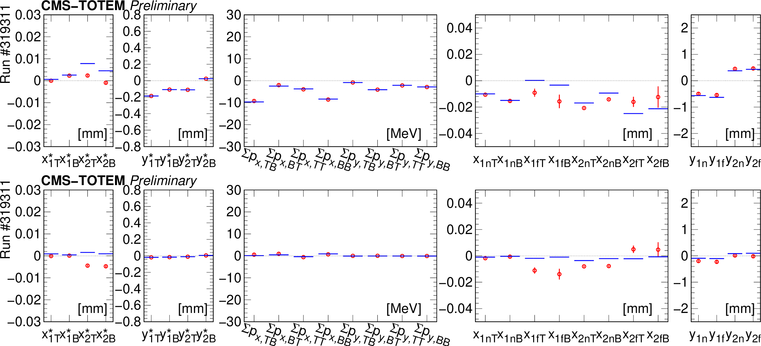
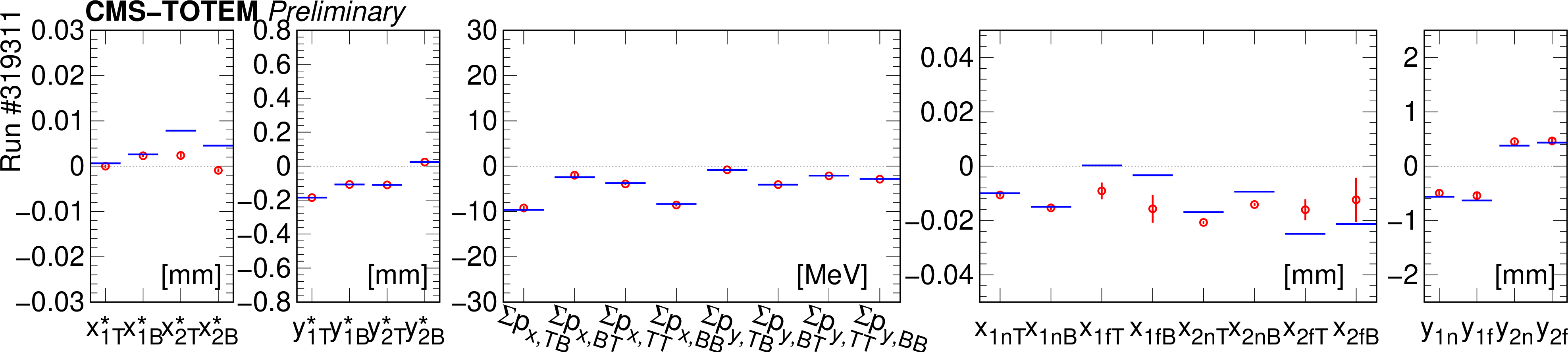
png pdf	Figure 17: The measured residuals (red symbols) and those expected from the extracted displacements (horizontal blue lines) for run \#319311, before (top) and after alignment (bottom).
png pdf	Figure 17-a: The measured residuals (red symbols) and those expected from the extracted displacements (horizontal blue lines) for run \#319311, before (top) and after alignment (bottom).
png pdf	Figure 17-b: The measured residuals (red symbols) and those expected from the extracted displacements (horizontal blue lines) for run \#319311, before (top) and after alignment (bottom).
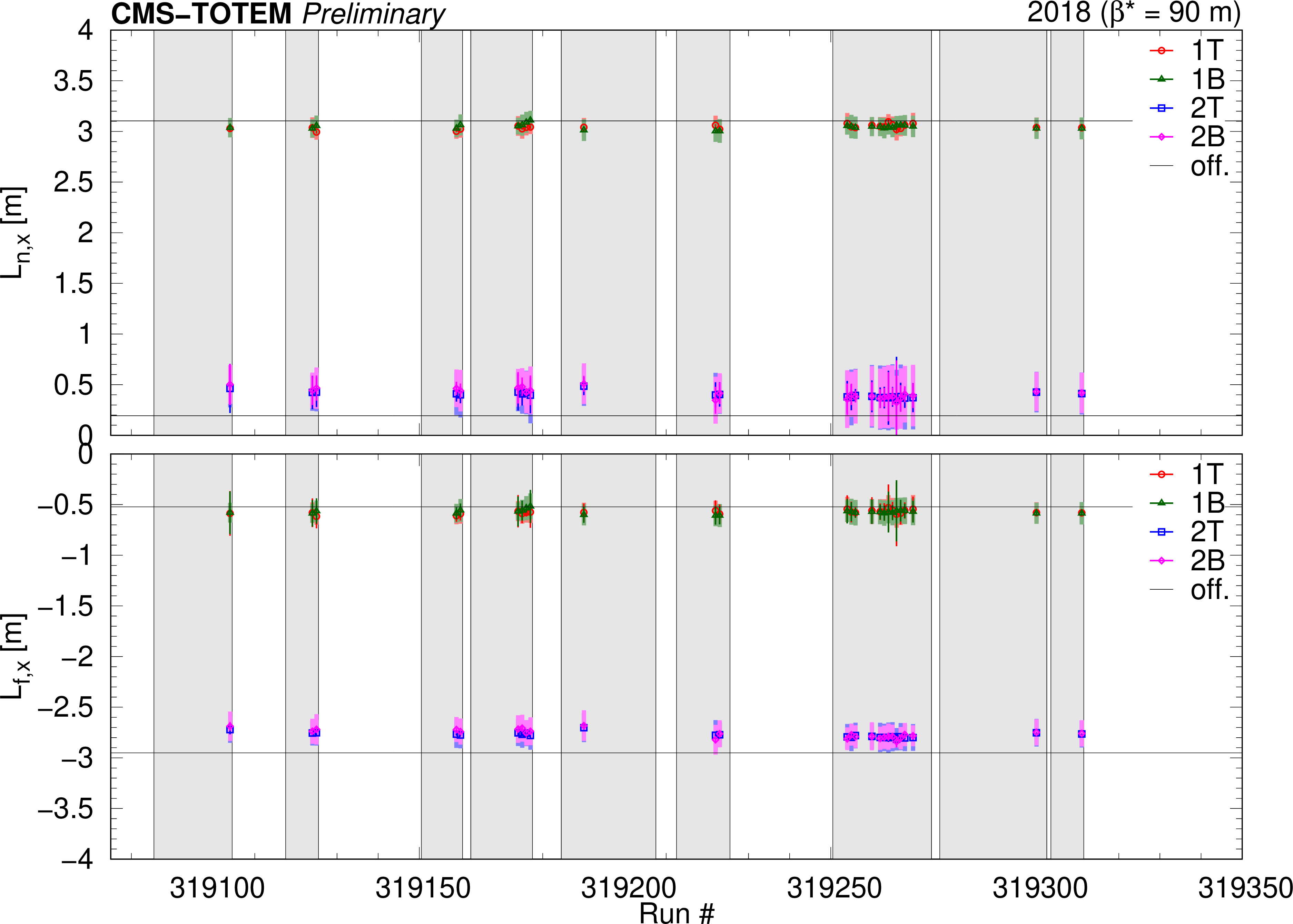
png pdf	Figure 18: Effective lengths at the location of the near ( $L_{n,x}$ ) and far pots ( $L_{f,x}$ ) as a function of run number, deduced from near-far hit covariances in RPs for RP arm configurations 1T, 1B, 2T, and 2B. Statistical uncertainties are indicated with error bars, systematic ones are plotted with shaded rectangles. Values of the nominal TOTEM optics parameters (Table 4) are also shown with black lines. LHC fills are indicated by grey areas.
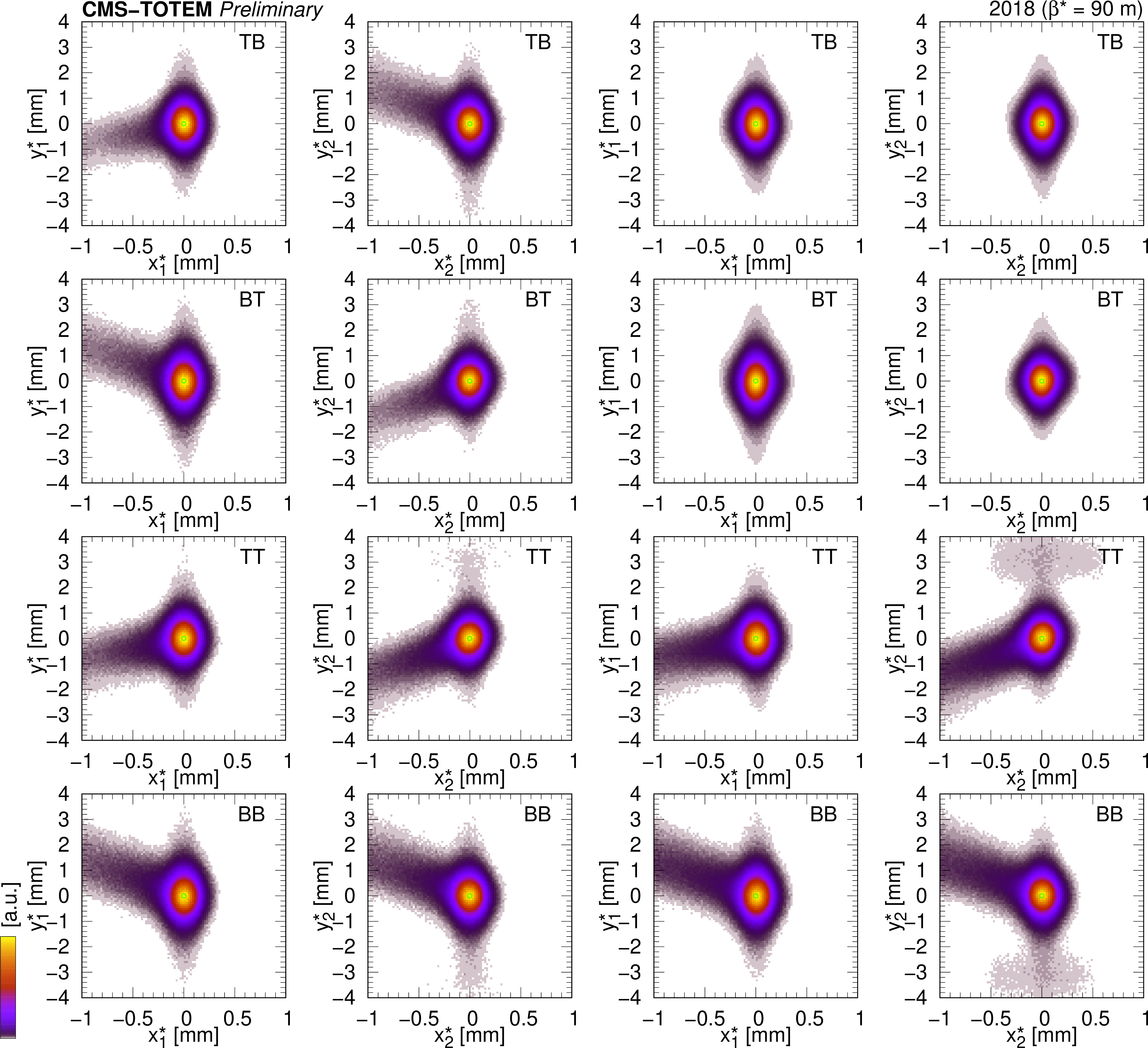
png pdf	Figure 19: Location of the primary pp interaction in the $x^$ - $y^$ plane at the IP using RPs in Arm 1 or 2 (subscripts 1 or 2), shown for various trigger configurations (TB, BT, TT, and BB, in rows). The two columns on the left side refer to the 2-track data set, whereas the two on the right side display distributions based on the 0-track data set. The elongated spots towards negative $x^*$ values correspond to non-exclusive events.
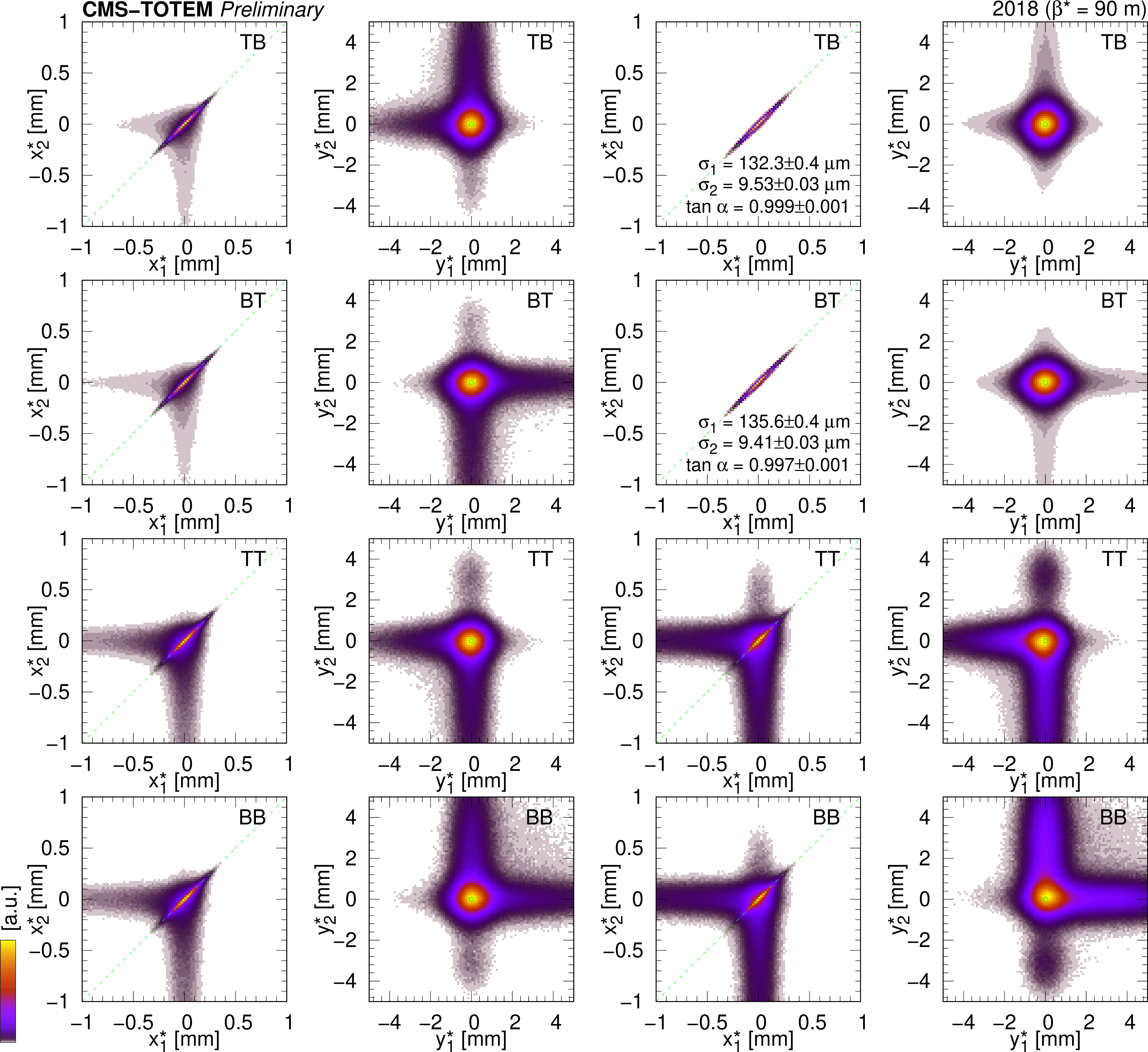
png pdf	Figure 20: Joint distribution of $x^$ (or $y^$ ) coordinates deduced using RPs in Arm 1 and 2 (subscripts 1 and 2), shown for various trigger configurations (TB, BT, TT, and BB, in rows). The two columns on the left side refer to the 2-track data set, whereas the two on the right side display distributions based on the 0-track data set. In the case of the diagonally triggered (TB and BT) 0-track (in part elastic) events the parameters (standard deviations in major and minor axis directions $\sigma_1$ and $\sigma_2$ , and the rotation angle $\alpha$ ) of the fitted ellipses are displayed in the plots. The green circles mark $(0,0)$ .
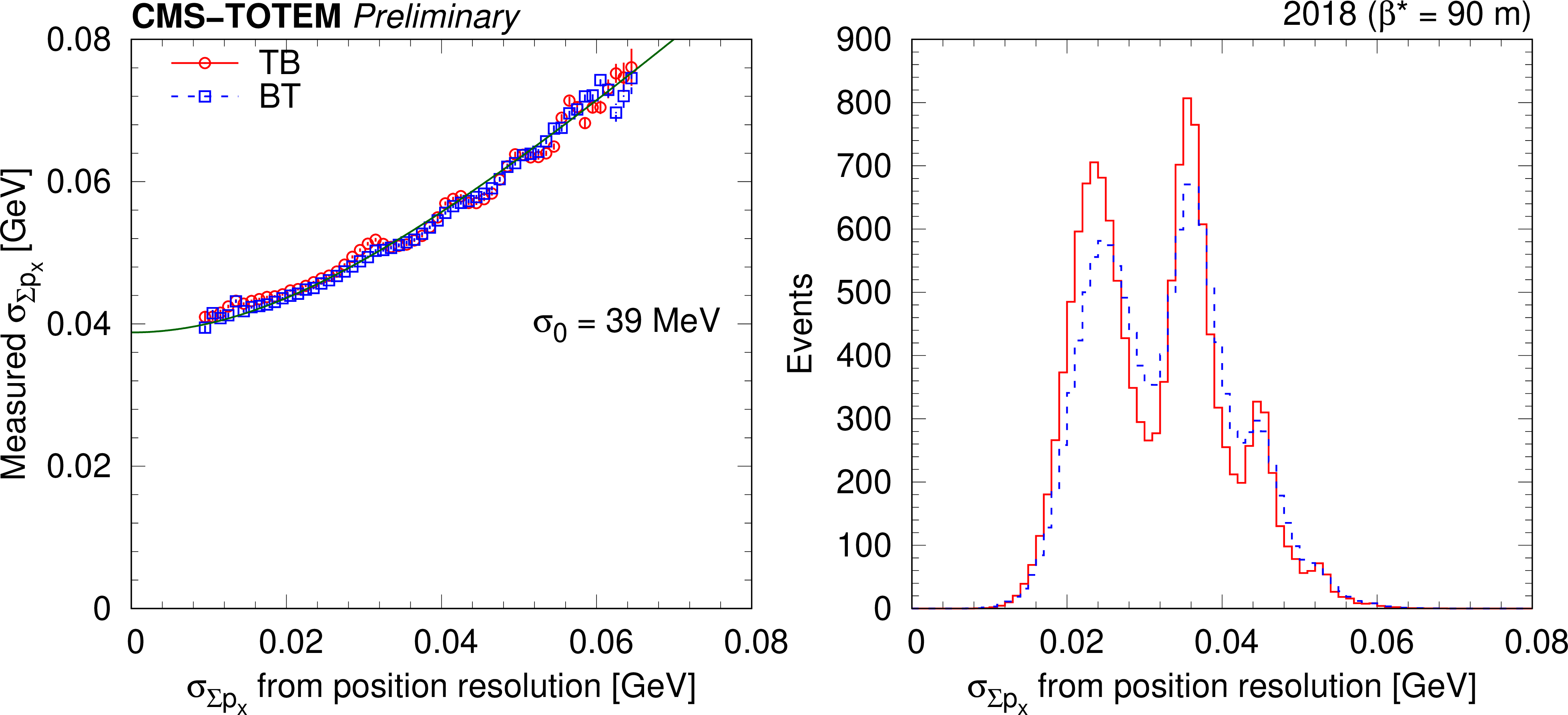
png pdf	Figure 21: Left: Standard deviation of momentum sum $\sum p_x$ for the 0-track data (TB and BT configurations), as a function of the predicted standard deviation from RP position resolution. A fit using the functional form $(\sigma_0^2 + \sigma_{\sum p_x}^2)^{1/2}$ is plotted with a green curve. Right: The occurrence of $\sigma_{\sum p_x}$ . The peaks correspond to events with protons leaving one or more two-strip clusters, and hence better resolution.
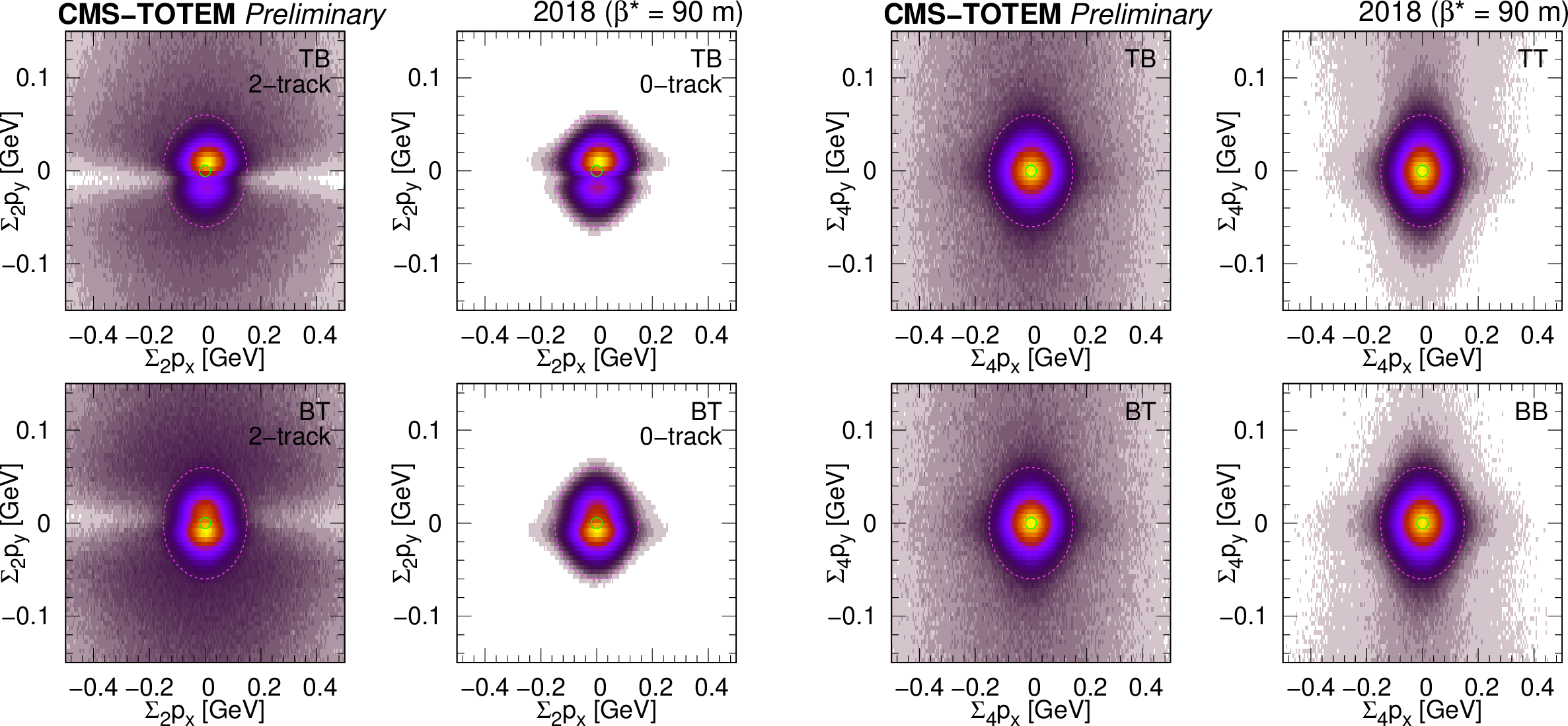
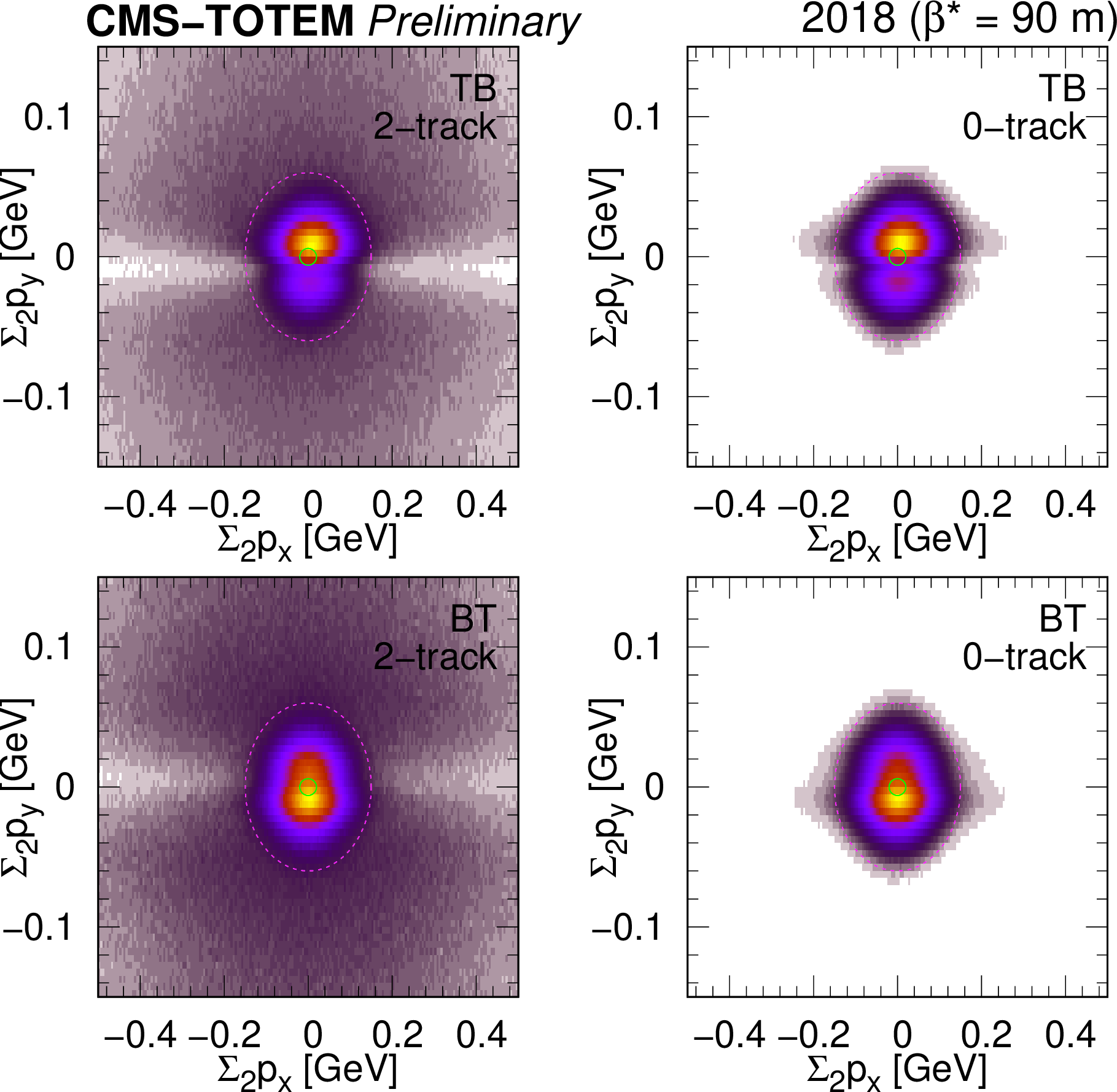
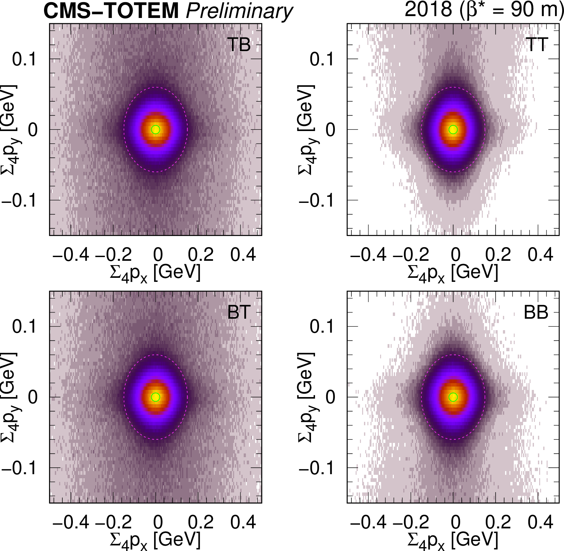
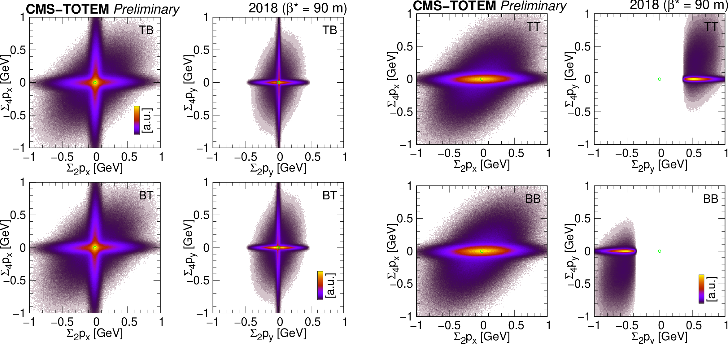
png pdf	Figure 22: Left: Distribution of the sum of scattered proton momenta $(\sum_2 p_x, \sum_2 p_y)$ for diagonally triggered events (TB and BT). The left column refers to the 2-track data set, whereas the right one displays the distribution based on the 0-track data set. Right: Distribution of the sum of scattered proton and central hadron momenta $(\sum_4 p_x, \sum_4 p_y)$ shown for various trigger configurations (TB, BT, TT, and BB) for 2-track events. Ellipses with semi-minor axes of 150 MeV ( $x$ ) and 60 MeV ( $y$ ) are overlaid.
png pdf	Figure 22-a: Left: Distribution of the sum of scattered proton momenta $(\sum_2 p_x, \sum_2 p_y)$ for diagonally triggered events (TB and BT). The left column refers to the 2-track data set, whereas the right one displays the distribution based on the 0-track data set. Right: Distribution of the sum of scattered proton and central hadron momenta $(\sum_4 p_x, \sum_4 p_y)$ shown for various trigger configurations (TB, BT, TT, and BB) for 2-track events. Ellipses with semi-minor axes of 150 MeV ( $x$ ) and 60 MeV ( $y$ ) are overlaid.
png pdf	Figure 22-b: Left: Distribution of the sum of scattered proton momenta $(\sum_2 p_x, \sum_2 p_y)$ for diagonally triggered events (TB and BT). The left column refers to the 2-track data set, whereas the right one displays the distribution based on the 0-track data set. Right: Distribution of the sum of scattered proton and central hadron momenta $(\sum_4 p_x, \sum_4 p_y)$ shown for various trigger configurations (TB, BT, TT, and BB) for 2-track events. Ellipses with semi-minor axes of 150 MeV ( $x$ ) and 60 MeV ( $y$ ) are overlaid.
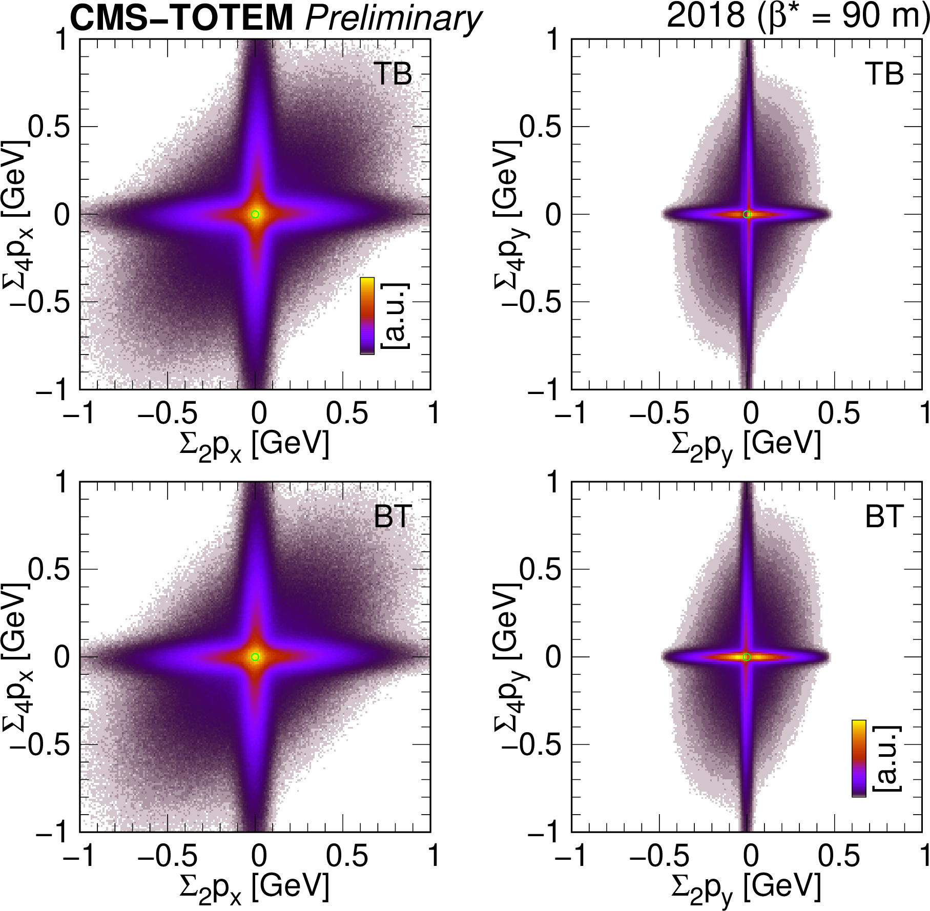
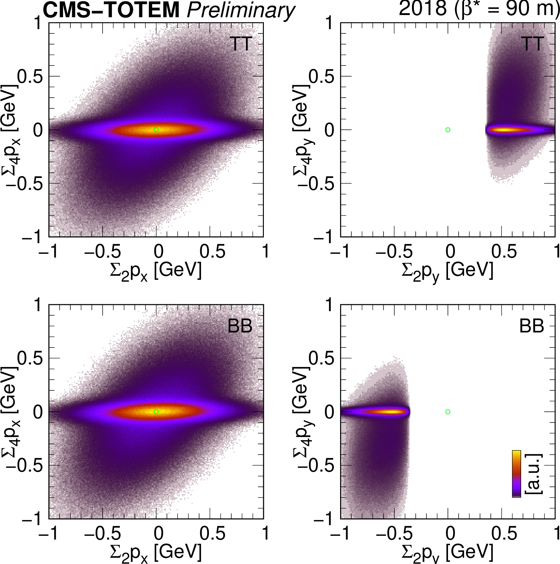
png pdf	Figure 23: Distribution of the sum of scattered proton and central hadron momenta and the sum of scattered proton momenta only ( $\sum_4 p_x$ and $\sum_2 p_x$ , $\sum_4 p_y$ and $\sum_2 p_y$ ) shown for various trigger configurations (TB, BT, TT, and BB) for 2-track events.
png pdf	Figure 23-a: Distribution of the sum of scattered proton and central hadron momenta and the sum of scattered proton momenta only ( $\sum_4 p_x$ and $\sum_2 p_x$ , $\sum_4 p_y$ and $\sum_2 p_y$ ) shown for various trigger configurations (TB, BT, TT, and BB) for 2-track events.
png pdf	Figure 23-b: Distribution of the sum of scattered proton and central hadron momenta and the sum of scattered proton momenta only ( $\sum_4 p_x$ and $\sum_2 p_x$ , $\sum_4 p_y$ and $\sum_2 p_y$ ) shown for various trigger configurations (TB, BT, TT, and BB) for 2-track events.

Tables
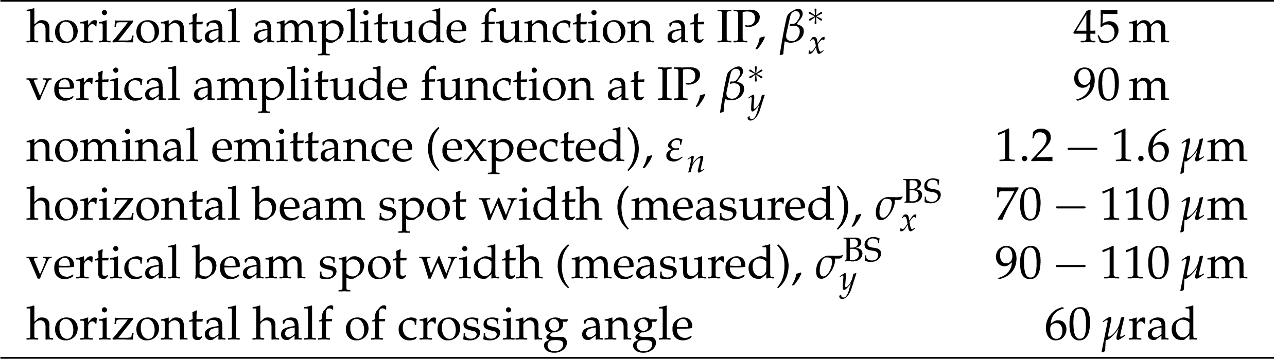
png pdf	Table 1: LHC beam parameters and related quantities for the $\beta^* =$ 90 m run at $\sqrt{s} =$ 13 TeV in 2018.
png pdf	Table 2: The naming of the various RP layer groups.
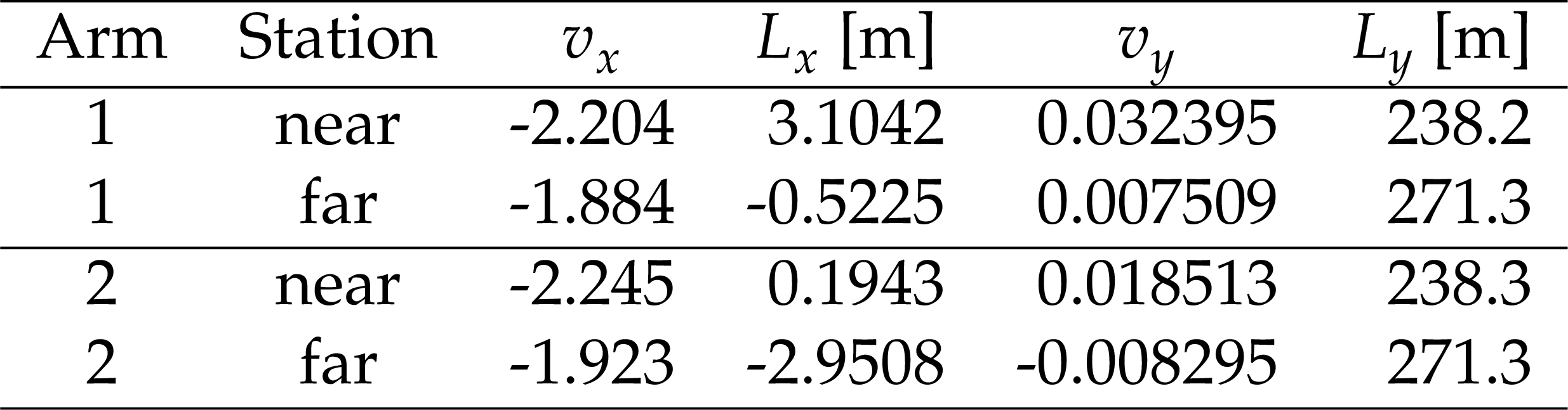
png pdf	Table 3: Nominal values of beam optics variables (magnifications $v$ , effective lengths $L$ ) [17,18], here truncated to four or five significant digits.
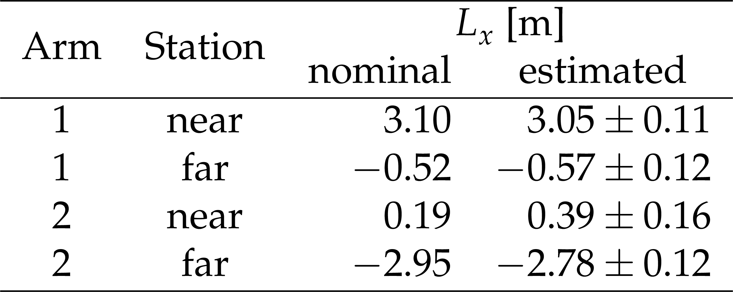
png pdf	Table 4: Nominal and data-driven estimates of effective lengths $L_x$ , here truncated to two decimal places. For the estimates, the systematic uncertainties are indicated, the statistical ones are negligible.

Summary

The Roman pot detectors of the TOTEM experiment are used to reconstruct the transverse momentum of scattered protons and to estimate the transverse location of the primary interaction. In this study advanced methods for local track reconstruction, measurements of strip-level detection efficiencies, cross-checks of beam optics, and steps of detector alignment are presented, along with their application in the selection of signal collision events. The local track reconstruction is performed by exploiting hit cluster information with a novel method, by finding a common polygonal area in the intercept-slope plane. As a result, the expected spatial resolution of 6-7

$\mu$ m is achieved. The tool is applied in the relative alignment of detector layers with

$\mu$ m precision. A tag-and-probe method is used to extract strip-level detection efficiencies. They are mostly constant, but for some strips they change with run number: there are up to 20% variations. The tracklet efficiencies are calculated using a probabilistic model, based on the run-by-run variation of the hit detection efficiencies. These are functions of the tracklet location and slope. There are up to 50% losses at specific but small areas, to be corrected for in the physics analysis. The absolute alignment of the RP system (8 numbers for each arm) is performed by means of 16 measured quantities in

$x$ , and 12 in

$y$ . The necessary run-by-run adjustments are in the range

$\pm$ 50

$\mu$ m in

$x$ , and

$\pm$ 0.5 mm in

$y$ . The deduced locations of the primary interaction, the distribution of the scattered proton momenta (global tracks), and their correlations confirm the success of the detailed calibration process and provide a solid ground for exclusive physics analyses based on the high-

$\beta^*$ data set. The methods described have been used in the physics analysis of central exclusive production events [22].

References
1	H. Wiedemann	Particle accelerator physics: basic principles and linear beam dynamics	Springer Berlin Heidelberg, . ISBN~978366039, 2013
2	TOTEM Collaboration	Timing measurements in the vertical Roman pots of the TOTEM experiment	CERN-LHCC-2014-020, TOTEM-TDR-002. \url https://cds.cern.ch/record/1753189, 2014
3	K. Österberg on behalf of the TOTEM Collaboration	Potential of central exclusive production studies in high $\beta^*$ runs at the LHC with CMS-TOTEM	Int. J. Mod. Phys. A 29 (2014) 1446019
4	M. G. Albrow, T. D. Coughlin, and J. R. Forshaw	Central exclusive particle production at high energy hadron colliders	Prog. Part. Nucl. Phys. 65 (2010) 149	1006.1289
5	H. Burkhardt	High-Beta Optics and Running Prospects	Instruments 3 (2019) 22
6	CMS Collaboration	The CMS experiment at the CERN LHC	JINST 3 (2008) S08004
7	TOTEM Collaboration	The TOTEM experiment at the CERN Large Hadron Collider	JINST 3 (2008) S08007
8	TOTEM Collaboration	Performance of the TOTEM Detectors at the LHC	Int. J. Mod. Phys. A 28 (2013) 1330046	1310.2908
9	Particle Data Group , R. L. Workman et al.	Review of particle physics	PTEP 2022 (2022) 083C01
10	CMS Collaboration	CMS luminosity measurement for the 2018 data-taking period at $\sqrt{s} =$ 13 TeV	CMS Physics Analysis Summary, 2018 CMS-PAS-LUM-18-002	CMS-PAS-LUM-18-002
11	CMS Collaboration	The CMS trigger system	JINST 12 (2017) P01020	CMS-TRG-12-001 1609.02366
12	R. Frühwirth	Application of Kalman filtering to track and vertex fitting	NIM A 262 (1987) 444
13	R. Frühwirth and A. Strandlie	Pattern recognition, tracking and vertex reconstruction in particle detectors	Particle Acceleration and Detection. Springer, 2020 ISBN 978-3-030-65770-3, 978-3-030-65771-0 link
14	CMS Collaboration	Measurements of inclusive W and Z cross sections in pp collisions at $\sqrt{s}=$ 7 TeV	JHEP 01 (2011) 080	CMS-EWK-10-002 1012.2466
15	J. A. Nelder and R. Mead	A simplex method for function minimization	Comput. J. 7 (1965) 308
16	J. Nocedal and S. Wright	Numerical optimization	Springer series in operations research and financial engineering. Springer, New York, 2d edition, ISBN~978-0-387-30303-1, 2006
17	TOTEM Collaboration	LHC optics measurement with proton tracks detected by the Roman pots of the TOTEM experiment	New J. Phys. 16 (2014) 103041	1406.0546
18	F. J. Nemes	Elastic scattering of protons at the TOTEM experiment at the LHC	PhD thesis, Eötvös U, 2015 link
19	W. Herr and F. Schmidt	A MAD-X primer	in CERN Accelerator School and DESY Zeuthen: Accelerator Physics, 2004
20	E. Wilson	An introduction to particle accelerators	Oxford Univ. Press, Oxford, 2001 ISBN~978008298
21	H. Niewiadomski	Reconstruction of protons in the TOTEM Roman pot detectors at the LHC	PhD thesis, Manchester U, 2008 link
22	CMS and TOTEM Collaborations	Nonresonant central exclusive production of charged-hadron pairs in proton-proton collisions at $\sqrt{s}$ = 13 TeV	PRD 109 (2024) 112013	CMS-SMP-21-004 2401.14494