

Compact Muon Solenoid
LHC, CERN
| CMS-SMP-23-006 ; CERN-EP-2024-273 | ||
| Proton reconstruction with the TOTEM Roman pot detectors for high-$ \beta^* $ LHC data | ||
| CMS Collaboration | ||
| 29 November 2024 | ||
| JINST 20 (2025) P04012 | ||
| Abstract: The TOTEM Roman pot detectors are used to reconstruct the transverse momentum of scattered protons and to estimate the transverse location of the primary interaction. This paper presents new methods of track reconstruction, measurements of strip-level detection efficiencies, cross-checks of the LHC beam optics, and detector alignment techniques, along with their application in the selection of signal collision events. The track reconstruction is performed by exploiting hit cluster information through a novel method using a common polygonal area in the intercept-slope plane. The technique is applied in the relative alignment of detector layers with $\mu$m precision. A tag-and-probe method is used to extract strip-level detection efficiencies. The alignment of the Roman pot system is performed through time-dependent adjustments, resulting in a position accuracy of 3 $\mu$m in the horizontal and 60 $\mu$m in the vertical directions. The goal is to provide an optimal reconstruction tool for central exclusive physics analyses based on the high-$ \beta^* $ data-taking period at $ \sqrt{s}= $ 13 TeV in 2018. | ||
| Links: e-print arXiv:2411.19749 [hep-ex] (PDF) ; CDS record ; inSPIRE record ; CADI line (restricted) ; | ||
| Figures | |

png pdf |
Figure 1:
Plan view of LHC section 56 (Arm 2) close to CMS (point 5 at the LHC). The location of the near and far Roman pots of Arm 2 are indicated in red. Also, various magnetic beam elements (dipoles D1 and 2, quadrupoles Q1 to Q6) as well as other Roman pots not used for this paper are shown. |
png pdf |
Figure 2:
Left: The eight RP units in Arm 1 and Arm 2 with the beam line, along with the location $ (x^*,y^*) $ of the primary interaction and two proton trajectories (dashed blue arrows), not to scale. Right: An RP unit comprising 10 layers with strips oriented alternately in the $ u $ and $ v $ directions. The blue dashed arrow represents an incoming proton. The axes of the local coordinate system are indicated with black solid arrows. |
png pdf |
Figure 2-a:
Left: The eight RP units in Arm 1 and Arm 2 with the beam line, along with the location $ (x^*,y^*) $ of the primary interaction and two proton trajectories (dashed blue arrows), not to scale. Right: An RP unit comprising 10 layers with strips oriented alternately in the $ u $ and $ v $ directions. The blue dashed arrow represents an incoming proton. The axes of the local coordinate system are indicated with black solid arrows. |
png pdf |
Figure 2-b:
Left: The eight RP units in Arm 1 and Arm 2 with the beam line, along with the location $ (x^*,y^*) $ of the primary interaction and two proton trajectories (dashed blue arrows), not to scale. Right: An RP unit comprising 10 layers with strips oriented alternately in the $ u $ and $ v $ directions. The blue dashed arrow represents an incoming proton. The axes of the local coordinate system are indicated with black solid arrows. |

png pdf |
Figure 3:
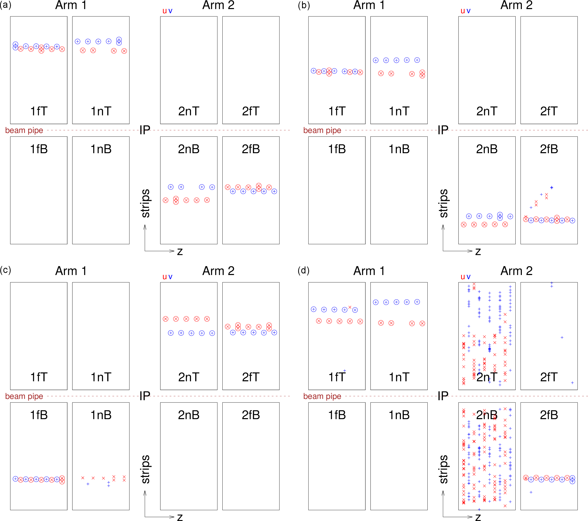
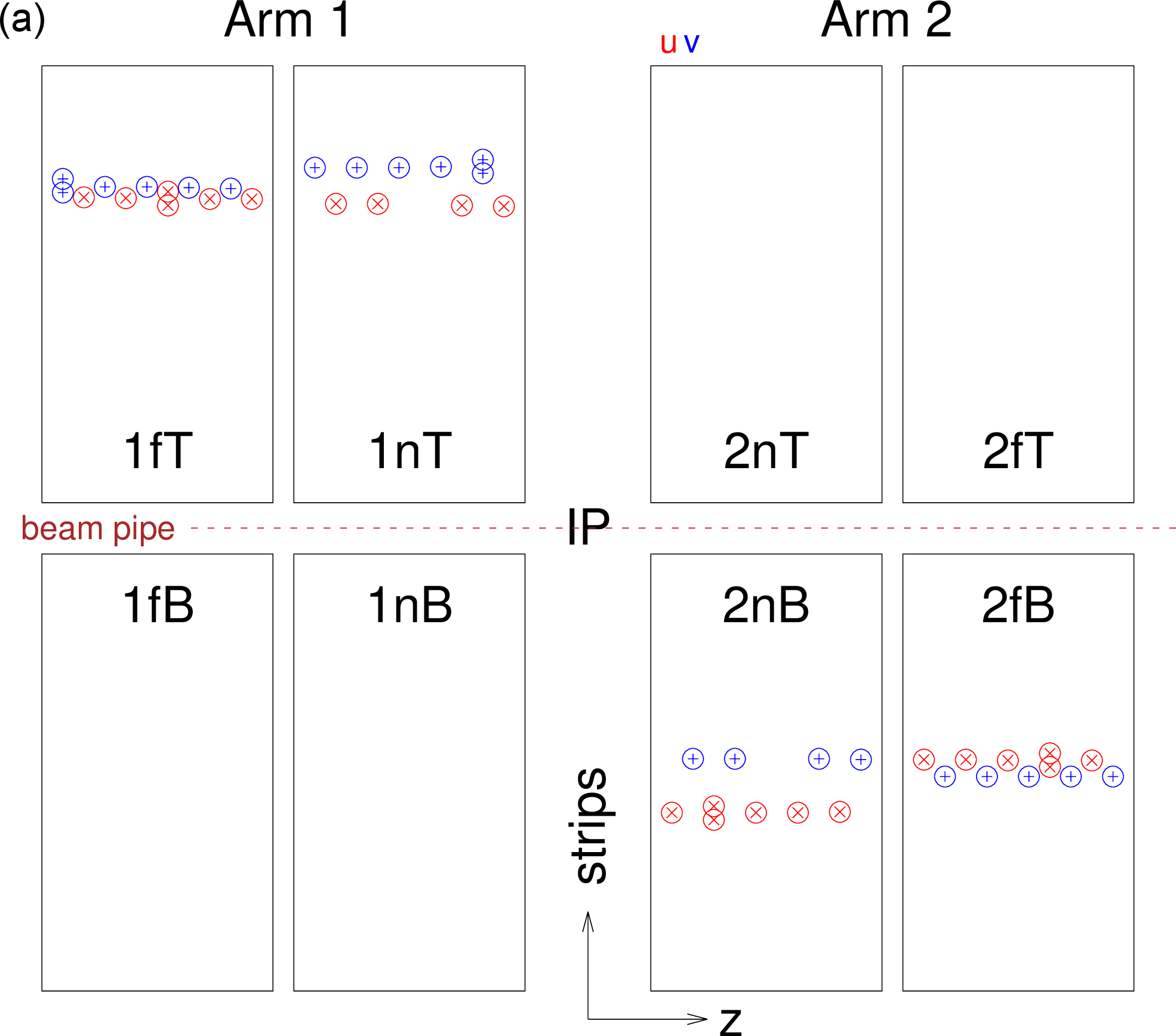
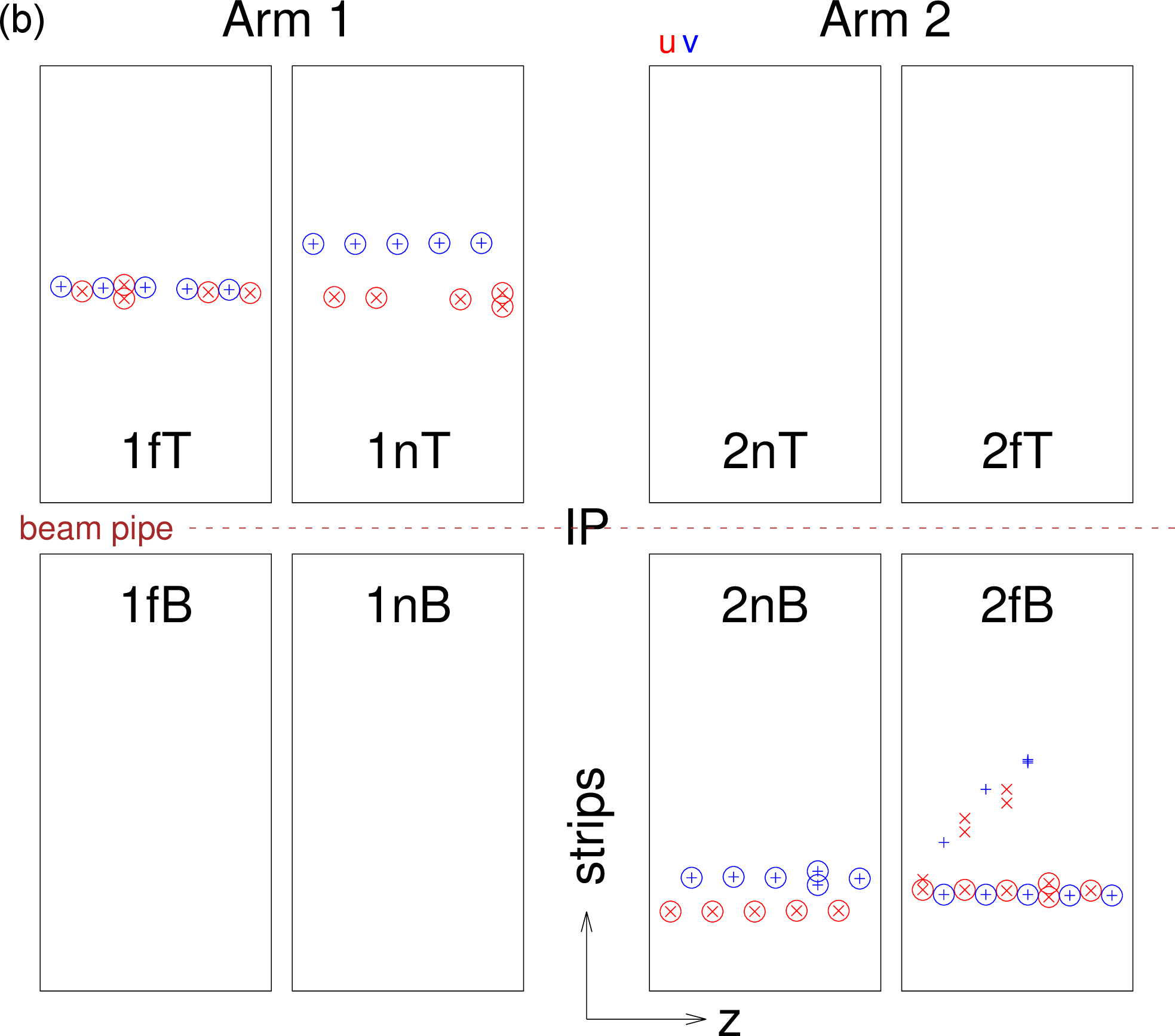
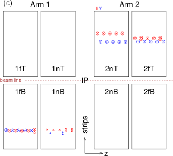
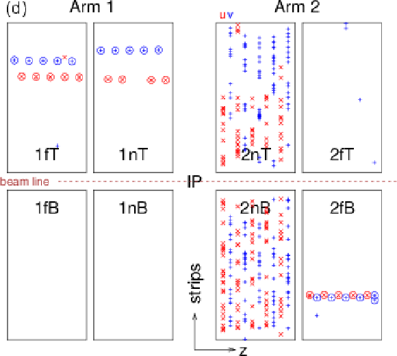
Schematic displays of four events with hits and projections of reconstructed local tracks (tracklets) in RPs, with outlines of Arm 1 and 2, near and far, upper and lower plots (not to scale). Strips of reconstructed clusters in $ u $ and $ v $ layers are plotted with red x and blue + markers, respectively. Two vertically adjacent symbols represent a two-strip cluster. Reconstructed clusters on a found tracklet are marked with circles. From left to right and from top to bottom: (a) normal event, (b) normal event with additional secondary particles; (c) not reconstructed event (less than three hits in the $ v $ orientation of 1n); (d) not reconstructed event (hadronic interaction in some beam element before 2n). |

png pdf |
Figure 3-a:
Schematic displays of four events with hits and projections of reconstructed local tracks (tracklets) in RPs, with outlines of Arm 1 and 2, near and far, upper and lower plots (not to scale). Strips of reconstructed clusters in $ u $ and $ v $ layers are plotted with red x and blue + markers, respectively. Two vertically adjacent symbols represent a two-strip cluster. Reconstructed clusters on a found tracklet are marked with circles. From left to right and from top to bottom: (a) normal event, (b) normal event with additional secondary particles; (c) not reconstructed event (less than three hits in the $ v $ orientation of 1n); (d) not reconstructed event (hadronic interaction in some beam element before 2n). |
png pdf |
Figure 3-b:
Schematic displays of four events with hits and projections of reconstructed local tracks (tracklets) in RPs, with outlines of Arm 1 and 2, near and far, upper and lower plots (not to scale). Strips of reconstructed clusters in $ u $ and $ v $ layers are plotted with red x and blue + markers, respectively. Two vertically adjacent symbols represent a two-strip cluster. Reconstructed clusters on a found tracklet are marked with circles. From left to right and from top to bottom: (a) normal event, (b) normal event with additional secondary particles; (c) not reconstructed event (less than three hits in the $ v $ orientation of 1n); (d) not reconstructed event (hadronic interaction in some beam element before 2n). |
png pdf |
Figure 3-c:
Schematic displays of four events with hits and projections of reconstructed local tracks (tracklets) in RPs, with outlines of Arm 1 and 2, near and far, upper and lower plots (not to scale). Strips of reconstructed clusters in $ u $ and $ v $ layers are plotted with red x and blue + markers, respectively. Two vertically adjacent symbols represent a two-strip cluster. Reconstructed clusters on a found tracklet are marked with circles. From left to right and from top to bottom: (a) normal event, (b) normal event with additional secondary particles; (c) not reconstructed event (less than three hits in the $ v $ orientation of 1n); (d) not reconstructed event (hadronic interaction in some beam element before 2n). |
png pdf |
Figure 3-d:
Schematic displays of four events with hits and projections of reconstructed local tracks (tracklets) in RPs, with outlines of Arm 1 and 2, near and far, upper and lower plots (not to scale). Strips of reconstructed clusters in $ u $ and $ v $ layers are plotted with red x and blue + markers, respectively. Two vertically adjacent symbols represent a two-strip cluster. Reconstructed clusters on a found tracklet are marked with circles. From left to right and from top to bottom: (a) normal event, (b) normal event with additional secondary particles; (c) not reconstructed event (less than three hits in the $ v $ orientation of 1n); (d) not reconstructed event (hadronic interaction in some beam element before 2n). |
png pdf |
Figure 4:
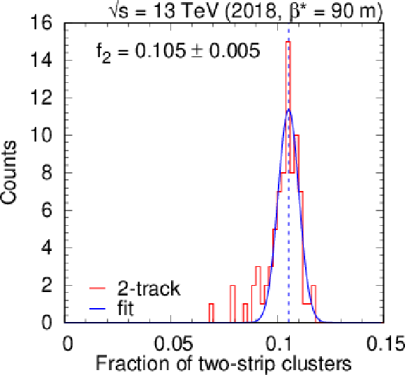
Left: Fraction of two-strip clusters for each detector layer, in groups of similarly oriented layers. Right: Distribution of the fraction of two-strip clusters with the result of a Gaussian fit. |
png pdf |
Figure 4-a:
Left: Fraction of two-strip clusters for each detector layer, in groups of similarly oriented layers. Right: Distribution of the fraction of two-strip clusters with the result of a Gaussian fit. |

png pdf |
Figure 4-b:
Left: Fraction of two-strip clusters for each detector layer, in groups of similarly oriented layers. Right: Distribution of the fraction of two-strip clusters with the result of a Gaussian fit. |

png pdf |
Figure 5:
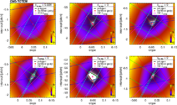
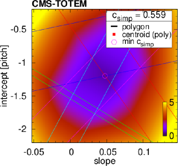
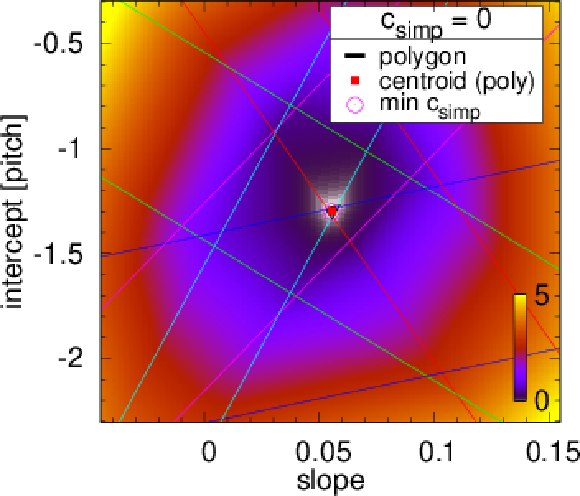
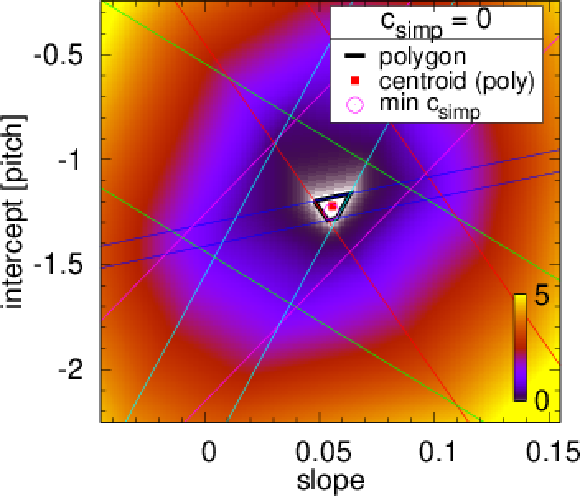
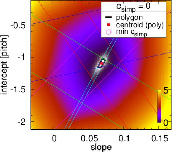
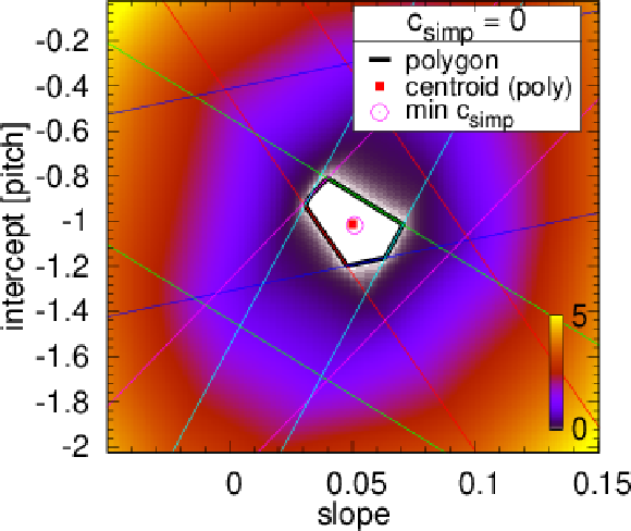
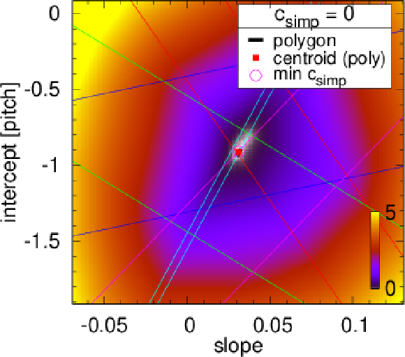
Examples of tracklet fits. The colour represents the value of the tracklet penalty function $ c $ in the intercept-slope ($ b-a $) plane. Bands corresponding to individual detector layers are shown with differently coloured parallel straight lines. The intersection of these bands, if it exists, is shown as a white polygonal area ($ c_\text{simp} = $ 0) framed with thick black lines, and its centroid is marked with a red filled square. If such intersection does not exist (top left subfigure), the result of the simplex minimisation $ c_\text{simp} > $ 0 is given, and the location of the minimum indicated with a purple open circle. |

png pdf |
Figure 5-a:
Examples of tracklet fits. The colour represents the value of the tracklet penalty function $ c $ in the intercept-slope ($ b-a $) plane. Bands corresponding to individual detector layers are shown with differently coloured parallel straight lines. The intersection of these bands, if it exists, is shown as a white polygonal area ($ c_\text{simp} = $ 0) framed with thick black lines, and its centroid is marked with a red filled square. If such intersection does not exist (top left subfigure), the result of the simplex minimisation $ c_\text{simp} > $ 0 is given, and the location of the minimum indicated with a purple open circle. |
png pdf |
Figure 5-b:
Examples of tracklet fits. The colour represents the value of the tracklet penalty function $ c $ in the intercept-slope ($ b-a $) plane. Bands corresponding to individual detector layers are shown with differently coloured parallel straight lines. The intersection of these bands, if it exists, is shown as a white polygonal area ($ c_\text{simp} = $ 0) framed with thick black lines, and its centroid is marked with a red filled square. If such intersection does not exist (top left subfigure), the result of the simplex minimisation $ c_\text{simp} > $ 0 is given, and the location of the minimum indicated with a purple open circle. |
png pdf |
Figure 5-c:
Examples of tracklet fits. The colour represents the value of the tracklet penalty function $ c $ in the intercept-slope ($ b-a $) plane. Bands corresponding to individual detector layers are shown with differently coloured parallel straight lines. The intersection of these bands, if it exists, is shown as a white polygonal area ($ c_\text{simp} = $ 0) framed with thick black lines, and its centroid is marked with a red filled square. If such intersection does not exist (top left subfigure), the result of the simplex minimisation $ c_\text{simp} > $ 0 is given, and the location of the minimum indicated with a purple open circle. |
png pdf |
Figure 5-d:
Examples of tracklet fits. The colour represents the value of the tracklet penalty function $ c $ in the intercept-slope ($ b-a $) plane. Bands corresponding to individual detector layers are shown with differently coloured parallel straight lines. The intersection of these bands, if it exists, is shown as a white polygonal area ($ c_\text{simp} = $ 0) framed with thick black lines, and its centroid is marked with a red filled square. If such intersection does not exist (top left subfigure), the result of the simplex minimisation $ c_\text{simp} > $ 0 is given, and the location of the minimum indicated with a purple open circle. |
png pdf |
Figure 5-e:
Examples of tracklet fits. The colour represents the value of the tracklet penalty function $ c $ in the intercept-slope ($ b-a $) plane. Bands corresponding to individual detector layers are shown with differently coloured parallel straight lines. The intersection of these bands, if it exists, is shown as a white polygonal area ($ c_\text{simp} = $ 0) framed with thick black lines, and its centroid is marked with a red filled square. If such intersection does not exist (top left subfigure), the result of the simplex minimisation $ c_\text{simp} > $ 0 is given, and the location of the minimum indicated with a purple open circle. |
png pdf |
Figure 5-f:
Examples of tracklet fits. The colour represents the value of the tracklet penalty function $ c $ in the intercept-slope ($ b-a $) plane. Bands corresponding to individual detector layers are shown with differently coloured parallel straight lines. The intersection of these bands, if it exists, is shown as a white polygonal area ($ c_\text{simp} = $ 0) framed with thick black lines, and its centroid is marked with a red filled square. If such intersection does not exist (top left subfigure), the result of the simplex minimisation $ c_\text{simp} > $ 0 is given, and the location of the minimum indicated with a purple open circle. |
png pdf |
Figure 6:
Deduced alignment parameters for inner layers ($ \delta_2 $ -- red circle, $ \delta_3 $ -- green triangle, $ \delta_4 $ -- blue square) in layer groups, in units of strip-width. Larger open symbols represent the 2-track data set, and the smaller ones are based on the 0-track data set. Shaded bars indicate the estimated systematic uncertainties (Section 3.2). |
png pdf |
Figure 7:
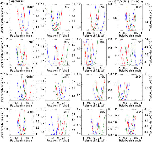
One-dimensional line scans of the relative shifts ($ \delta_2 $ -- red, $ \delta_3 $ -- green, $ \delta_4 $ -- blue) for the 16 layer groups around the best values found. The joint $ c $ value is plotted as a function of the relative shifts of the inner layers around the found minima (solid curves, left vertical scale). Goodness-of-fit from an alternative method, counting tracks with $ c = $ 0, is also indicated (dashed lines, right vertical scale, number of such tracks with inverted axis). In the 1nTu panel (upper left corner) the curve corresponding to the third layer is missing since that layer is inefficient. |

png pdf |
Figure 8:
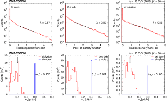
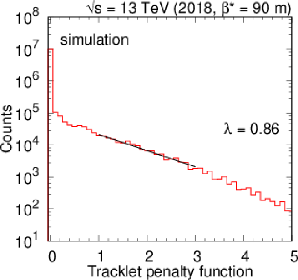
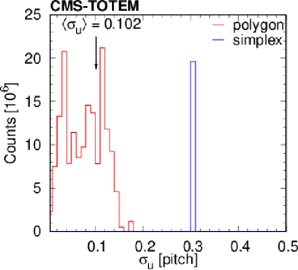
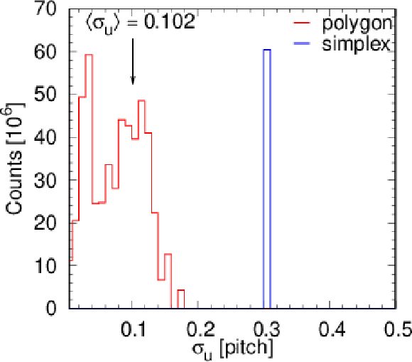
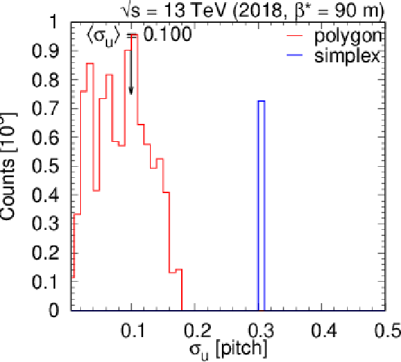
Upper: Distribution of the tracklet penalty function with the slope $ \lambda $ of an exponential fit (black line) in the range 1--3. Lower: Distribution of the standard deviation of the fitted hit location in strip-width units for the polygon method (red), and for those cases where the simplex minimisation was necessary (blue, at 0.3). The three columns correspond to the 0-track (left), 2-track (centre), and the simulated (right) data sets. The vertical arrow indicates the location of the average value. |

png pdf |
Figure 8-a:
Upper: Distribution of the tracklet penalty function with the slope $ \lambda $ of an exponential fit (black line) in the range 1--3. Lower: Distribution of the standard deviation of the fitted hit location in strip-width units for the polygon method (red), and for those cases where the simplex minimisation was necessary (blue, at 0.3). The three columns correspond to the 0-track (left), 2-track (centre), and the simulated (right) data sets. The vertical arrow indicates the location of the average value. |

png pdf |
Figure 8-b:
Upper: Distribution of the tracklet penalty function with the slope $ \lambda $ of an exponential fit (black line) in the range 1--3. Lower: Distribution of the standard deviation of the fitted hit location in strip-width units for the polygon method (red), and for those cases where the simplex minimisation was necessary (blue, at 0.3). The three columns correspond to the 0-track (left), 2-track (centre), and the simulated (right) data sets. The vertical arrow indicates the location of the average value. |
png pdf |
Figure 8-c:
Upper: Distribution of the tracklet penalty function with the slope $ \lambda $ of an exponential fit (black line) in the range 1--3. Lower: Distribution of the standard deviation of the fitted hit location in strip-width units for the polygon method (red), and for those cases where the simplex minimisation was necessary (blue, at 0.3). The three columns correspond to the 0-track (left), 2-track (centre), and the simulated (right) data sets. The vertical arrow indicates the location of the average value. |
png pdf |
Figure 8-d:
Upper: Distribution of the tracklet penalty function with the slope $ \lambda $ of an exponential fit (black line) in the range 1--3. Lower: Distribution of the standard deviation of the fitted hit location in strip-width units for the polygon method (red), and for those cases where the simplex minimisation was necessary (blue, at 0.3). The three columns correspond to the 0-track (left), 2-track (centre), and the simulated (right) data sets. The vertical arrow indicates the location of the average value. |
png pdf |
Figure 8-e:
Upper: Distribution of the tracklet penalty function with the slope $ \lambda $ of an exponential fit (black line) in the range 1--3. Lower: Distribution of the standard deviation of the fitted hit location in strip-width units for the polygon method (red), and for those cases where the simplex minimisation was necessary (blue, at 0.3). The three columns correspond to the 0-track (left), 2-track (centre), and the simulated (right) data sets. The vertical arrow indicates the location of the average value. |
png pdf |
Figure 8-f:
Upper: Distribution of the tracklet penalty function with the slope $ \lambda $ of an exponential fit (black line) in the range 1--3. Lower: Distribution of the standard deviation of the fitted hit location in strip-width units for the polygon method (red), and for those cases where the simplex minimisation was necessary (blue, at 0.3). The three columns correspond to the 0-track (left), 2-track (centre), and the simulated (right) data sets. The vertical arrow indicates the location of the average value. |
png pdf |
Figure 9:
Strip hit efficiency from data, determined with a tag-and-probe method. Shown here are layer 5 in layer group 1nTv (top) and 2nBu (bottom) for a specific run. Values and statistical uncertainties based on the 2-track data set (red symbols) and those from 0-track data (blue symbols) are plotted. The borders of the front-end chips are indicated with (green) vertical lines. The uncertainties are large at the left or the right sides of the layers, because those regions are rarely hit. |

png pdf |
Figure 9-a:
Strip hit efficiency from data, determined with a tag-and-probe method. Shown here are layer 5 in layer group 1nTv (top) and 2nBu (bottom) for a specific run. Values and statistical uncertainties based on the 2-track data set (red symbols) and those from 0-track data (blue symbols) are plotted. The borders of the front-end chips are indicated with (green) vertical lines. The uncertainties are large at the left or the right sides of the layers, because those regions are rarely hit. |

png pdf |
Figure 9-b:
Strip hit efficiency from data, determined with a tag-and-probe method. Shown here are layer 5 in layer group 1nTv (top) and 2nBu (bottom) for a specific run. Values and statistical uncertainties based on the 2-track data set (red symbols) and those from 0-track data (blue symbols) are plotted. The borders of the front-end chips are indicated with (green) vertical lines. The uncertainties are large at the left or the right sides of the layers, because those regions are rarely hit. |
png pdf |
Figure 10:
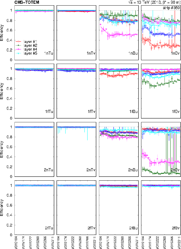
Strip hit efficiencies as functions of the run number for strip \#350 in layers 1--5 (coloured points) in various layer groups (labels in the lower right corner). Statistical uncertainties are indicated with vertical bars. Lines are spline interpolations to guide the eye. |
png pdf |
Figure 11:
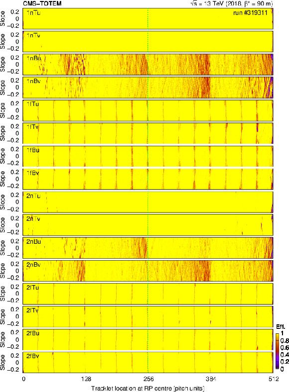
Tracklet reconstruction efficiency (colour scale) as a function of tracklet location at the centre of the RP (intercept) and the track slope, for a representative run, shown for each layer group separately. Yellow regions correspond to fully efficient tracklet reconstruction, whereas the red regions exhibit substantial losses with efficiencies in the range 0.4--0.6. Vertical green lines denote boundaries of the front-end chips. |
png pdf |
Figure 12:
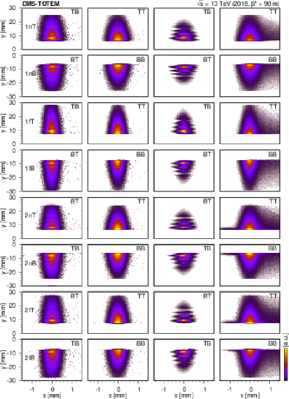
Efficiency-corrected distribution of proton hit locations in the $ x-y $ plane at the references surfaces of the eight RPs (rows), for different trigger configurations (labels at the upper right corner). The two columns on the left side refer to the 2-track data set, whereas the two on the right side display distributions based on the 0-track data set. The wavy pattern and the halo seen in the 0-track data set is explained in the text. |
png pdf |
Figure 13:
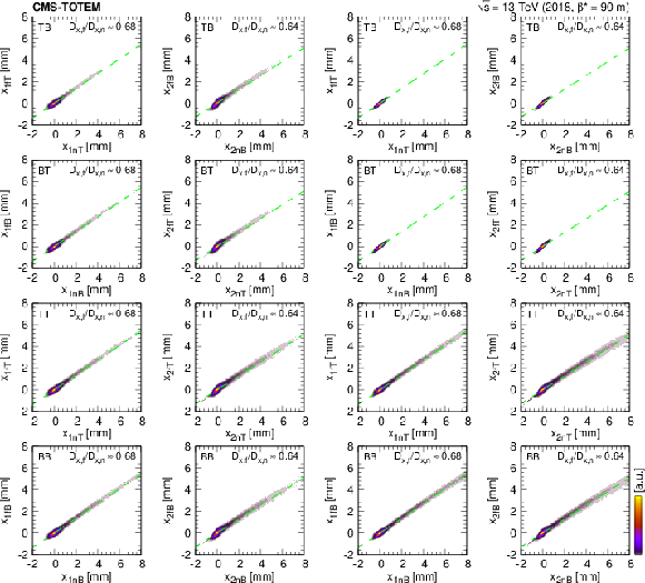
Correlation of proton hit locations in the $ x $ direction (two-dimensional occupancy histograms) in the far and near RPs, shown for various trigger configurations (TB, BT, TT, and BB, in rows). The two columns on the left side refer to the 2-track data set, and the two on the right side display distributions based on the 0-track data set. A straight line corresponding to the expectation $ x_\mathrm{f} = x_\mathrm{n} \, D_{x,\mathrm{f}}/D_{x,\mathrm{n}} $ is also plotted, where $ D_{x,f}/D_{x,n} \approx $ 0.68 for Arm 1, and $ \approx $ 0.64 for Arm 2. The plots are produced with the final detector alignment. |
png pdf |
Figure 14:
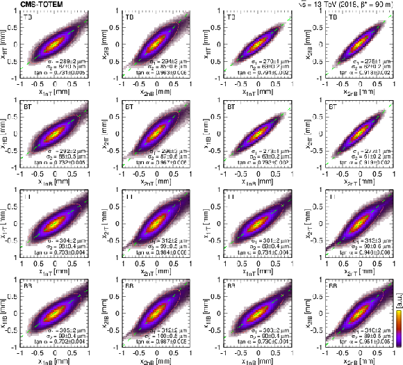
Correlation of proton hit locations in the $ x $ direction (two-dimensional occupancy histograms) in the far and near RPs, shown for various trigger configurations (TB, BT, TT, and BB, in rows), with a restricted scale. Parameters (standard deviations in major and minor axis directions $ \sigma_1 $ and $ \sigma_2 $, and the rotation angle $ \alpha $) of the fitted tilted two-dimensional normal distributions are displayed in the plots. The corresponding ellipses cover 99% of the points; the dashed green lines indicate their major axes. The two columns on the left side refer to the 2-track data set, whereas the two on the right side display distributions based on the 0-track data set. The plots are produced with the final detector alignment. |
png pdf |
Figure 15:
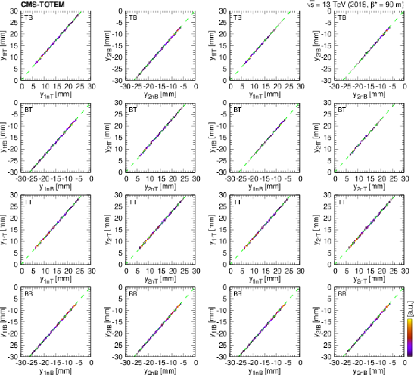
Correlation of proton hit locations in the $ y $ direction (two-dimensional occupancy histograms) in the far and near RPs, shown for various trigger configurations (TB, BT, TT, and BB, in rows). The two columns on the left side refer to the 2-track data set, whereas the two on the right side display distributions based on the 0-track data set. A straight line corresponding to the expectation $ y_\mathrm{f} = y_\mathrm{n} \, L_{y,\mathrm{f}}/L_{y,\mathrm{n}} $ is also plotted, where $ L_{y,f}/L_{y,n} \approx $ 1.14. The plots are produced with the final detector alignment. The apparent piecewise linear segments are simply the consequence of the binning. |
png pdf |
Figure 16:
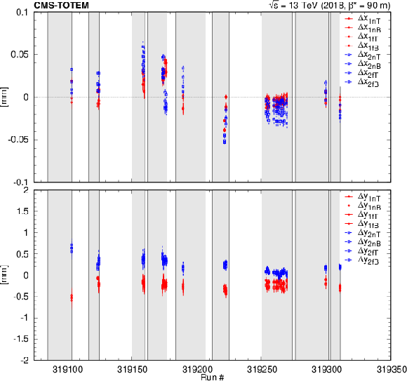
Deduced displacements of RPs in the $ x $ (top) and $ y $ (bottom) directions as a function of run number. Statistical uncertainties are shown with vertical bars. The LHC fills are indicated by grey areas. |

png pdf |
Figure 17:
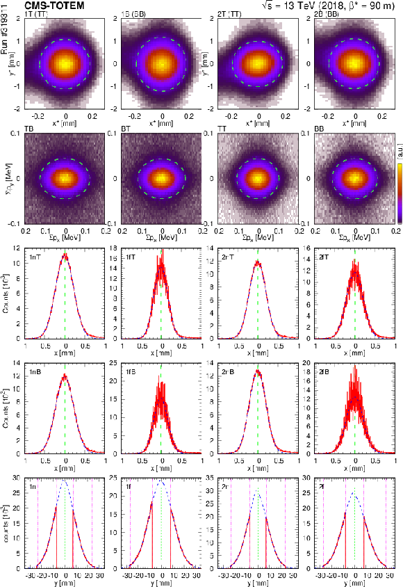
Cross-check of the full alignment, shown here for run \#319311. From top to bottom: Distribution of the IP coordinates $ (x^*,y^*) $ for RP arm configurations 1T, 1B, 2T, and 2B. Distribution of the four-particle momentum sum $ (\sum p_x,\sum p_y) $ for the RP trigger configurations TB, BT, TT, and BB. In both cases the two-dimensional Gaussian fits are indicated (at 2 $ \sigma $) with green dotted ellipses. Distribution of local hits in the RPs in the $ x $ (single Gaussian) and $ y $ directions (separate Gaussians). Dashed blue curves represent the Gaussian fits, vertical green dashed lines indicate the deduced relative shifts, vertical magenta dash-dotted lines on $ y $ plots show fit ranges. |
png pdf |
Figure 18:
The measured residuals (red symbols) and those expected from the extracted displacements (horizontal blue lines) for run \#319311, before (upper) and after (lower) the alignment. |

png pdf |
Figure 18-a:
The measured residuals (red symbols) and those expected from the extracted displacements (horizontal blue lines) for run \#319311, before (upper) and after (lower) the alignment. |

png pdf |
Figure 18-b:
The measured residuals (red symbols) and those expected from the extracted displacements (horizontal blue lines) for run \#319311, before (upper) and after (lower) the alignment. |
png pdf |
Figure 19:
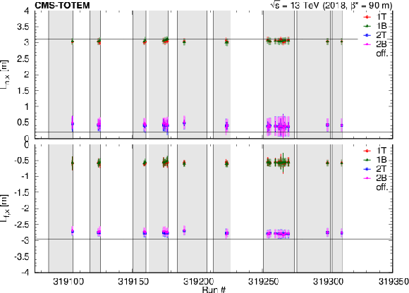
Effective lengths at the location of the near ($ L_{n,x} $) and far pots ($ L_{f,x} $) as functions of the run number, deduced from near-far hit covariances in RPs for RP arm configurations 1T, 1B, 2T, and 2B. Statistical uncertainties are indicated with error bars, systematic ones are plotted with shaded rectangles. Values of the nominal TOTEM optics parameters (Table 4) are also shown with horizontal black lines. LHC fills are indicated by grey areas. |

png pdf |
Figure 20:
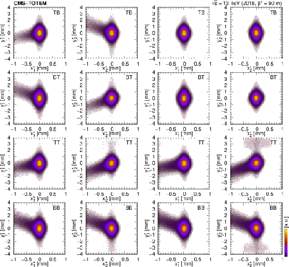
Location of the primary pp interaction in the $ x^*-y^* $ plane at the IP using RPs in Arm 1 or 2 (subscripts 1 or 2), shown for various trigger configurations (TB, BT, TT, and BB, in rows). The two columns on the left side refer to the 2-track data set, whereas the two on the right side display distributions based on the 0-track data set. The elongated regions at negative $ x^* $ values correspond to events with large proton momentum loss. The green circles mark $ (0,0) $. |
png pdf |
Figure 21:
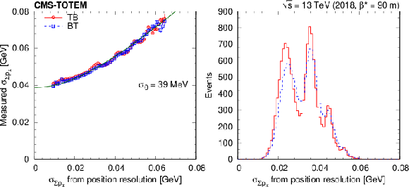
Joint distribution of $ x^* $ (or $ y^* $) coordinates deduced using RPs in Arm 1 and 2 (subscripts 1 and 2), shown for various trigger configurations (TB, BT, TT, and BB, in rows). The two columns on the left side refer to the 2-track data set, whereas the two on the right side display distributions based on the 0-track data set. In the case of the diagonally triggered (TB and BT) 0-track (in part elastic) events the parameters (standard deviations in major and minor axis directions $ \sigma_1 $ and $ \sigma_2 $, and the rotation angle $ \alpha $) of the fitted ellipses are displayed in the plots. The green circles mark $ (0,0) $, the dashed green lines are the identity lines. |
png pdf |
Figure 22:
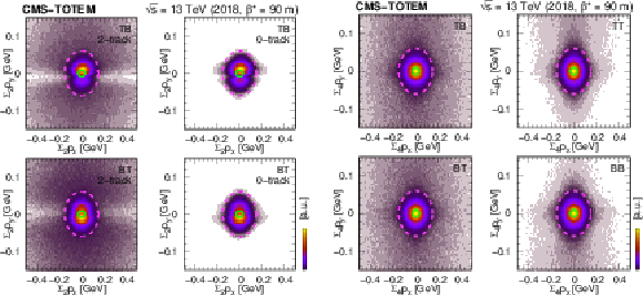
Left: Standard deviation of the momentum sum $ \sum p_x $ for the 0-track data (TB and BT configurations), as a function of the predicted standard deviation from the RP position resolution. Statistical uncertainties are shown with vertical bars. A fit using the functional form $ (\sigma_0^2 + \sigma_{\sum p_x}^2)^{1/2} $ is plotted with a green curve. Right: The occurrence of $ \sigma_{\sum p_x} $. The peaks correspond to events with protons causing one or more two-strip clusters, and hence better resolution. |
png pdf |
Figure 23:
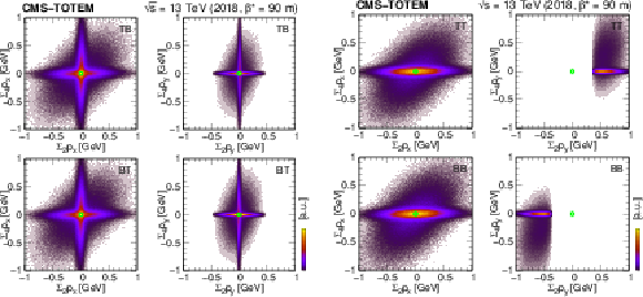
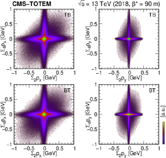
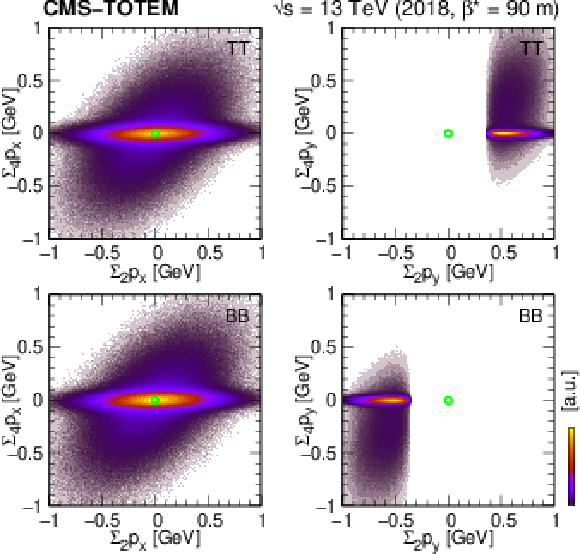
Left: Distribution of the sum of scattered proton momenta $ (\sum_2 p_x, \sum_2 p_y) $ for diagonally triggered events (TB and BT). The left column refers to the 2-track data set, whereas the right one displays the distribution based on the 0-track data set. Right: Distribution of the sum of scattered proton and central hadron momenta $ (\sum_4 p_x, \sum_4 p_y) $ shown for various trigger configurations (TB, BT, TT, and BB) for 2-track events. Ellipses with semi-minor axes of 150 MeV ($ x $) and 60 MeV ($ y $) are overlaid. The green circles mark $ (0,0) $. |
png pdf |
Figure 23-a:
Left: Distribution of the sum of scattered proton momenta $ (\sum_2 p_x, \sum_2 p_y) $ for diagonally triggered events (TB and BT). The left column refers to the 2-track data set, whereas the right one displays the distribution based on the 0-track data set. Right: Distribution of the sum of scattered proton and central hadron momenta $ (\sum_4 p_x, \sum_4 p_y) $ shown for various trigger configurations (TB, BT, TT, and BB) for 2-track events. Ellipses with semi-minor axes of 150 MeV ($ x $) and 60 MeV ($ y $) are overlaid. The green circles mark $ (0,0) $. |
png pdf |
Figure 23-b:
Left: Distribution of the sum of scattered proton momenta $ (\sum_2 p_x, \sum_2 p_y) $ for diagonally triggered events (TB and BT). The left column refers to the 2-track data set, whereas the right one displays the distribution based on the 0-track data set. Right: Distribution of the sum of scattered proton and central hadron momenta $ (\sum_4 p_x, \sum_4 p_y) $ shown for various trigger configurations (TB, BT, TT, and BB) for 2-track events. Ellipses with semi-minor axes of 150 MeV ($ x $) and 60 MeV ($ y $) are overlaid. The green circles mark $ (0,0) $. |
png pdf |
Figure 24:
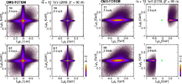
Distribution of the sum of scattered proton and central hadron momenta and the sum of scattered proton momenta only ($ \sum_4 p_x $ and $ \sum_2 p_x $, $ \sum_4 p_y $ and $ \sum_2 p_y $) shown for various trigger configurations (TB, BT, TT, and BB) for 2-track events. The green circles mark $ (0,0) $. |
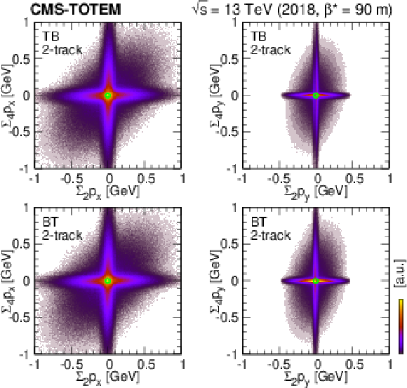
png pdf |
Figure 24-a:
Distribution of the sum of scattered proton and central hadron momenta and the sum of scattered proton momenta only ($ \sum_4 p_x $ and $ \sum_2 p_x $, $ \sum_4 p_y $ and $ \sum_2 p_y $) shown for various trigger configurations (TB, BT, TT, and BB) for 2-track events. The green circles mark $ (0,0) $. |
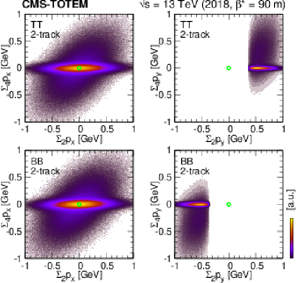
png pdf |
Figure 24-b:
Distribution of the sum of scattered proton and central hadron momenta and the sum of scattered proton momenta only ($ \sum_4 p_x $ and $ \sum_2 p_x $, $ \sum_4 p_y $ and $ \sum_2 p_y $) shown for various trigger configurations (TB, BT, TT, and BB) for 2-track events. The green circles mark $ (0,0) $. |
| Tables | |
png pdf |
Table 1:
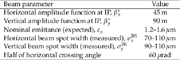
The beam parameters and related quantities at the CMS interaction point for the $ \beta^* = $ 90 m run at $ \sqrt{s}= $ 13 TeV in 2018. |

png pdf |
Table 2:
The naming of the various RP layer groups. |

png pdf |
Table 3:
Nominal values of beam optics variables (magnifications $ v $, effective lengths $ L $) [19,20], truncated to four or five significant digits. |
png pdf |
Table 4:
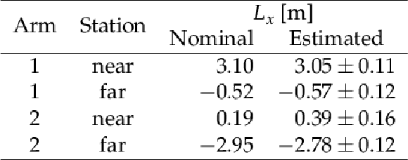
Nominal values and estimates of the effective lengths $ L_x $, truncated to two decimal places. For the estimates, the systematic uncertainties are indicated; the statistical ones are negligible. |
| Summary |
| The Roman pot detectors of the TOTEM experiment are used to reconstruct the transverse momentum of scattered protons and to estimate the transverse location of the primary interaction. In this study advanced methods for track reconstruction, measurements of strip-level detection efficiencies, cross-checks of beam optics, and the detector alignment procedure are presented, along with their application in the selection of signal events. The track reconstruction is performed by finding a common polygonal area in the intercept-slope plane, thus exploiting all available cluster information. As a result, an ultimate spatial resolution of 6 $ -$7 $\mu$m is achieved, which is an order of magnitude smaller than the strip width. The tool is applied to the relative alignment of detector layers with $\mu$m precision. A tag-and-probe method is used to extract strip-level detection efficiencies. They are mostly high and constant, but for some strips they change with time; there are up to 20% variations. The tracklet efficiencies are calculated using a probabilistic model, based on the temporal variation of the hit detection efficiencies. These are functions of the tracklet location and slope. There are up to 50% losses in specific but small areas, to be corrected in the physics analyses. The alignment of the Roman pot system (8 numbers for each arm) is performed by means of 16 measured quantities in the horizontal, and 12 in the vertical direction, resulting in a position accuracy of 3 $\mu$m in the horizontal and 60 $\mu$m in the vertical directions. The deduced locations of the primary interaction, the distribution of the scattered proton momenta, and their correlations confirm the success of the detailed calibration process and provide a solid ground for exclusive physics analyses based on the high-$ \beta^* $ data set. The developed methods have been successfully applied in the analysis of central exclusive production events [3]. |
| References | ||||
| 1 | TOTEM Collaboration | Timing measurements in the vertical Roman pots of the TOTEM experiment | CERN-LHCC-2014-020, TOTEM-TDR-002 | |
| 2 | K. Österberg on behalf of the TOTEM Collaboration | Potential of central exclusive production studies in high $ \beta^* $ runs at the LHC with CMS-TOTEM | Int. J. Mod. Phys. A 29 (2014) 1446019 | |
| 3 | CMS and TOTEM Collaborations | Nonresonant central exclusive production of charged-hadron pairs in proton-proton collisions at $ \sqrt{s} $ = 13 TeV | PRD 109 (2024) 112013 | CMS-SMP-21-004 2401.14494 |
| 4 | CMS Collaboration | CMS luminosity measurement for the 2018 data-taking period at $ \sqrt{s} = $ 13 TeV | CMS Physics Analysis Summary, 2018 CMS-PAS-LUM-18-002 |
CMS-PAS-LUM-18-002 |
| 5 | H. Wiedemann | Particle accelerator physics: basic principles and linear beam dynamics | Springer Berlin Heidelberg, ISBN 978366039, 2013 | |
| 6 | M. G. Albrow, T. D. Coughlin, and J. R. Forshaw | Central exclusive particle production at high energy hadron colliders | Prog. Part. Nucl. Phys. 65 (2010) 149 | 1006.1289 |
| 7 | H. Burkhardt | High-beta optics and running prospects | Instruments 3 (2019) 22 | |
| 8 | CMS Collaboration | The CMS experiment at the CERN LHC | JINST 3 (2008) S08004 | |
| 9 | TOTEM Collaboration | The TOTEM experiment at the CERN Large Hadron Collider | JINST 3 (2008) S08007 | |
| 10 | TOTEM Collaboration | Performance of the TOTEM Detectors at the LHC | Int. J. Mod. Phys. A 28 (2013) 1330046 | 1310.2908 |
| 11 | Particle Data Group, S. Navas et al. | Review of particle physics | PRD 110 (2024) 030001 | |
| 12 | CMS Collaboration | The CMS trigger system | JINST 12 (2017) P01020 | CMS-TRG-12-001 1609.02366 |
| 13 | R. Frühwirth | Application of Kalman filtering to track and vertex fitting | NIM A 262 (1987) 444 | |
| 14 | P. Billoir and S. Qian | Simultaneous pattern recognition and track fitting by the Kalman filtering method | NIM A 294 (1990) 219 | |
| 15 | R. Frühwirth and A. Strandlie | Pattern recognition, tracking and vertex reconstruction in particle detectors | Particle Acceleration and Detection. Springer, ISBN 978-3-030-65770-3, 978-3-030-65771-0, 2020 link |
|
| 16 | CMS Collaboration | Measurements of inclusive W and Z cross sections in pp collisions at $ \sqrt{s}= $ 7 TeV | JHEP 01 (2011) 080 | CMS-EWK-10-002 1012.2466 |
| 17 | C. Steger | On the calculation of arbitrary moments of polygons | Technical Report FGBV-96-05, Forschungsgruppe Bildverstehen (FG BV), Informatik IX, Technische Universität München, 1996 link |
|
| 18 | J. A. Nelder and R. Mead | A simplex method for function minimization | Comput. J. 7 (1965) 308 | |
| 19 | TOTEM Collaboration | LHC optics measurement with proton tracks detected by the Roman pots of the TOTEM experiment | New J. Phys. 16 (2014) 103041 | 1406.0546 |
| 20 | F. J. Nemes | Elastic scattering of protons at the TOTEM experiment at the LHC | PhD thesis, Eötvös U., CERN-THESIS-2015-293, 2015 link |
|
| 21 | W. Herr and F. Schmidt | A MAD-X primer | in CERN Accelerator School and DESY Zeuthen: Accelerator Physics, CERN-AB-2004-027-ABP, 2004 | |
| 22 | E. Wilson | An introduction to particle accelerators | Oxford Univ. Press, Oxford, ISBN 978008298, 2001 link |
|
| 23 | H. Niewiadomski | Reconstruction of protons in the TOTEM Roman pot detectors at the LHC | PhD thesis, Manchester U., CERN-THESIS-2008-080, 2008 link |
|

|
Compact Muon Solenoid LHC, CERN |

|

|

|

|

|

|