

Compact Muon Solenoid
LHC, CERN
| CMS-PAS-SMP-22-007 | ||
| Measurement of the primary Lund jet plane density in proton-proton collisions at $ \sqrt{s} = $ 13 TeV | ||
| CMS Collaboration | ||
| 25 March 2023 | ||
| Abstract: A measurement of the primary Lund jet plane density in inclusive jet production in proton-proton collisions is presented. The analysis uses 138 fb$ ^{-1} $ of data collected by the CMS experiment at $ \sqrt{s} = $ 13 TeV. The Lund jet plane, a representation of the phase space of emissions inside jets, is extracted using iterative jet declustering. The transverse momentum $ k_\mathrm{T} $ and the splitting angle $ \Delta R $ of an emission relative to its emitter are measured at each step of the jet declustering process. The average density of emissions in $ \ln(k_\mathrm{T}/\mathrm{GeV}) $ and $ \ln (R/\Delta R) $ is measured for jets with distance parameters $ R = $ 0.4 or 0.8 and transverse momentum $ p_\mathrm{T} > $ 700 GeV and rapidity $ |y| < $ 1.7. The jet substructure is extracted using the charged-particle tracks of the jet to achieve optimal momentum and angular resolution. The measured distributions are unfolded to the level of stable particles. The measurement is compared with theoretical predictions from state-of-the-art simulations. | ||
|
Links:
CDS record (PDF) ;
Physics Briefing ;
CADI line (restricted) ;
These preliminary results are superseded in this paper, Submitted to JHEP. The superseded preliminary plots can be found here. |
||
| Figures | |

png pdf |
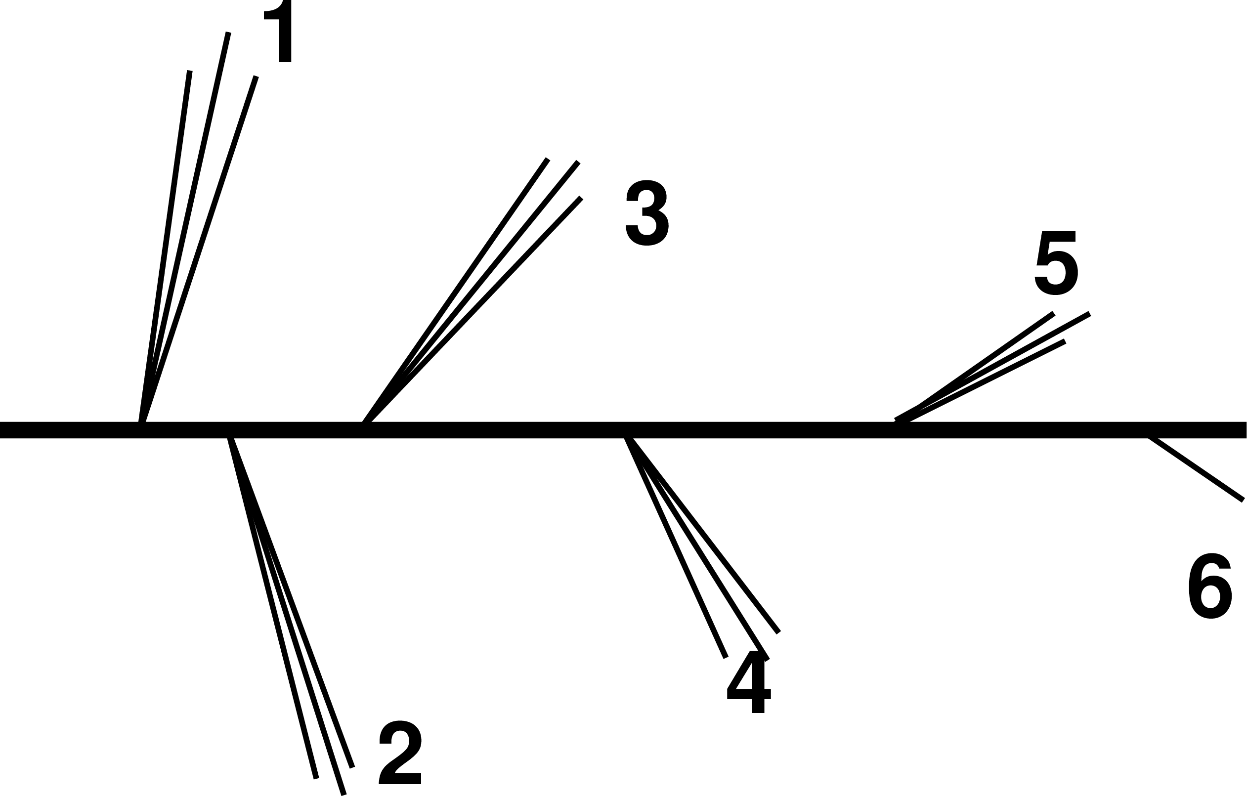
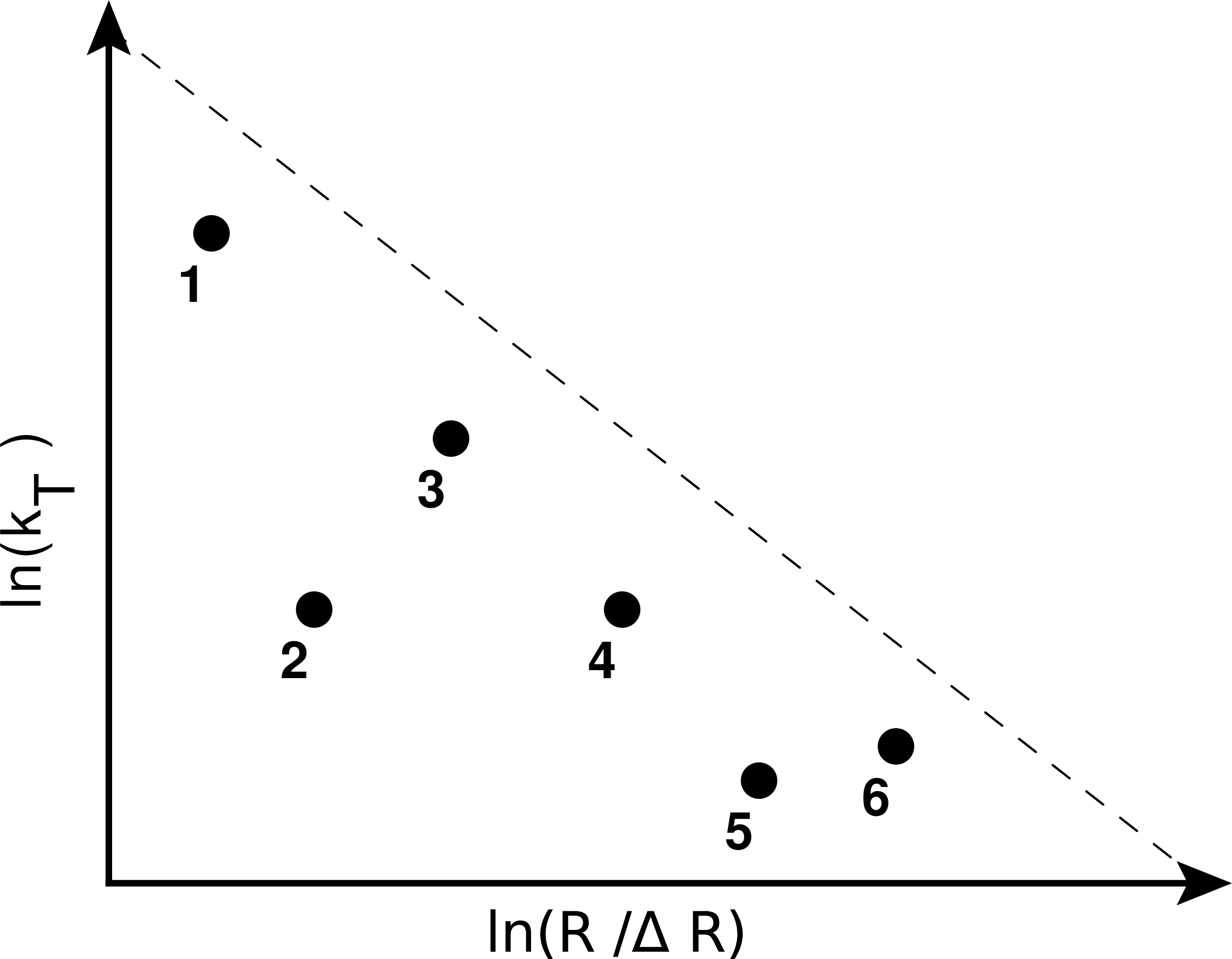
Figure 1:
(Left) Schematic diagram of the Cambridge/Aachen primary declustering tree of a jet. The emissions are angular ordered, as indicated with the numbers in the diagram. (Right) Schematic diagram of the primary emissions of a jet in the Lund jet plane. The Lund jet plane is filled from left to right, which corresponds to emissions ordered from large angles to small angles. The dashed line represents the kinematical limit. |
png pdf |
Figure 1-a:
(Left) Schematic diagram of the Cambridge/Aachen primary declustering tree of a jet. The emissions are angular ordered, as indicated with the numbers in the diagram. (Right) Schematic diagram of the primary emissions of a jet in the Lund jet plane. The Lund jet plane is filled from left to right, which corresponds to emissions ordered from large angles to small angles. The dashed line represents the kinematical limit. |
png pdf |
Figure 1-b:
(Left) Schematic diagram of the Cambridge/Aachen primary declustering tree of a jet. The emissions are angular ordered, as indicated with the numbers in the diagram. (Right) Schematic diagram of the primary emissions of a jet in the Lund jet plane. The Lund jet plane is filled from left to right, which corresponds to emissions ordered from large angles to small angles. The dashed line represents the kinematical limit. |
png pdf |
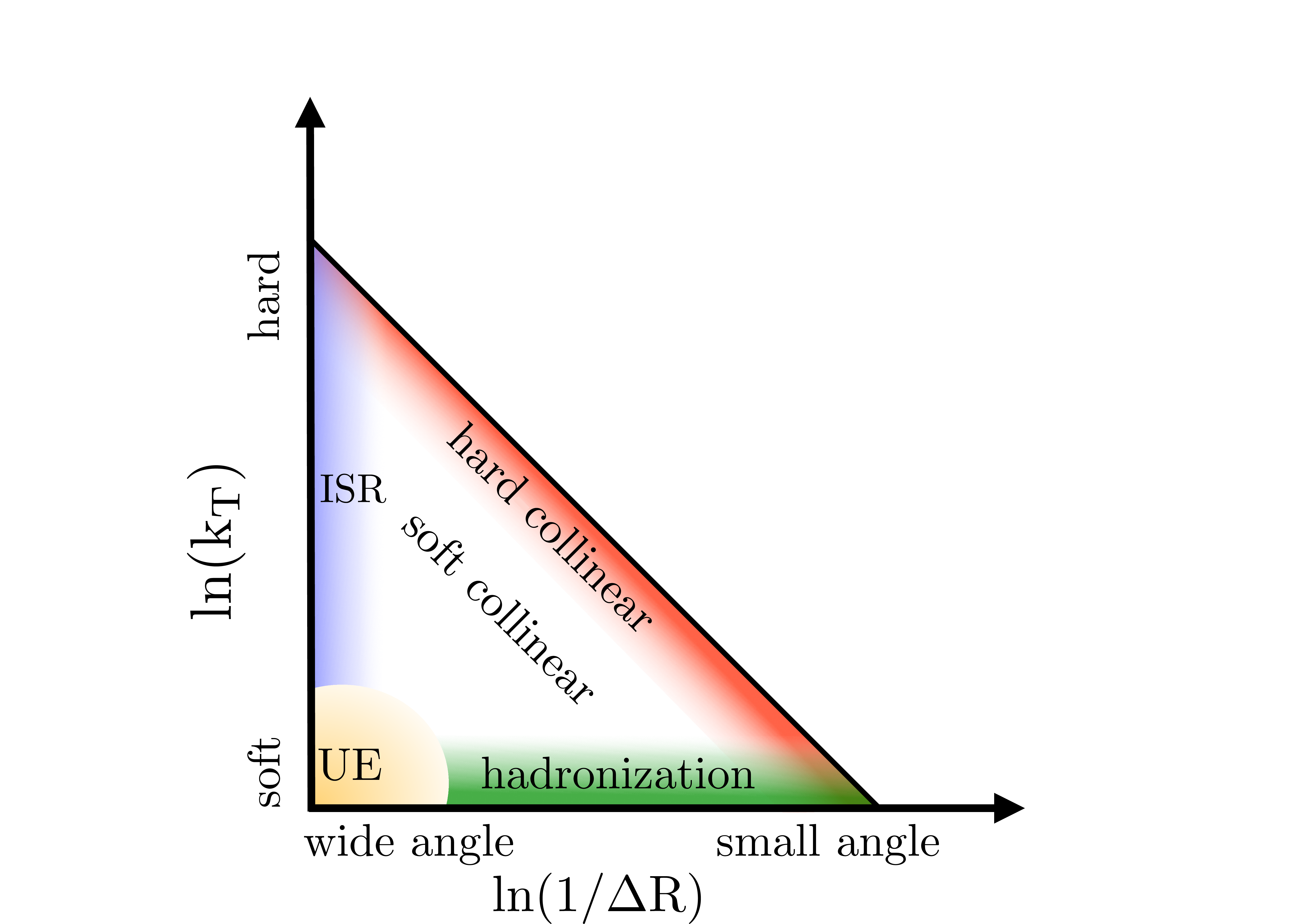
Figure 2:
Schematic diagram of the physical effects affecting different regions of the primary Lund jet plane. Initial-state radiation (ISR) and the underlying event (UE) activity affect wide angle radiation. Hadronization affects the low $ \ln(k_{\mathrm{T}}/\,\text{GeV}) $ region at all angles. Soft and hard collinear parton splittings affect the rest of the Lund jet plane. The diagonal line represents the kinematical limit of the primary Lund jet plane, which corresponds to $ p_{\mathrm{T}}^\mathrm{j1} = p_{\mathrm{T}}^\mathrm{j2} $. |
png pdf |
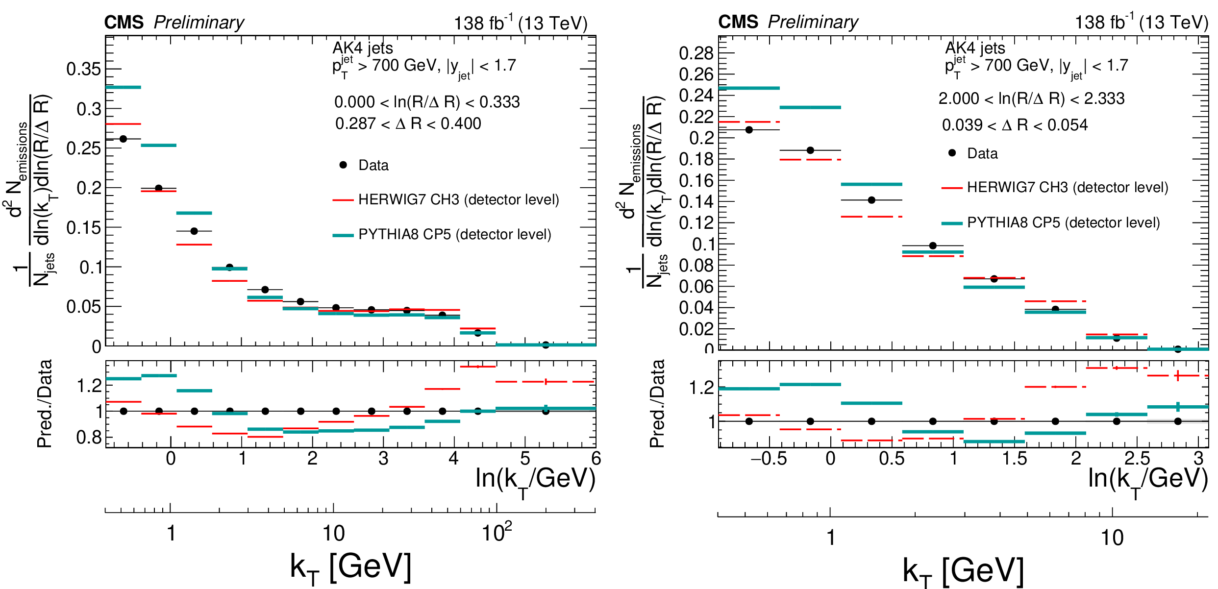
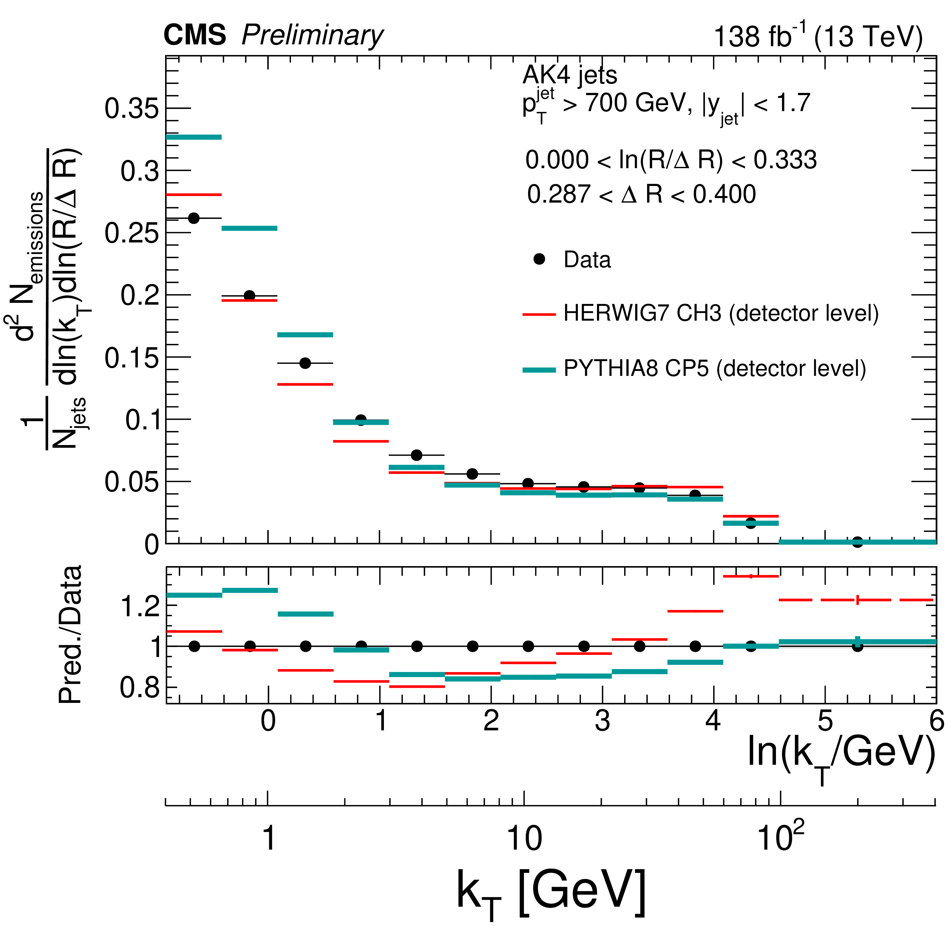
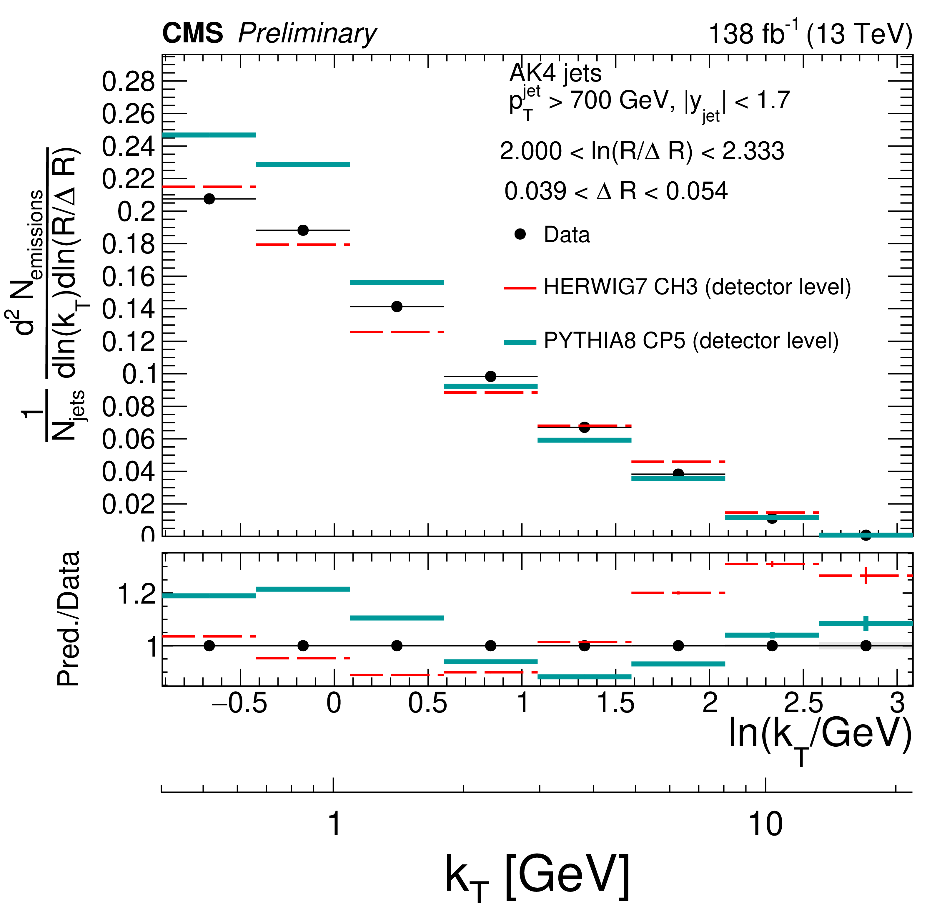
Figure 3:
Detector-level distributions of data and Monte Carlo simulated events generated with PYTHIA8 CP5 and HERWIG 7 CH3. The lower panels show the ratio of the predictions with respect to the data. Only statistical uncertainties are included here. |
png pdf |
Figure 3-a:
Detector-level distributions of data and Monte Carlo simulated events generated with PYTHIA8 CP5 and HERWIG 7 CH3. The lower panels show the ratio of the predictions with respect to the data. Only statistical uncertainties are included here. |
png pdf |
Figure 3-b:
Detector-level distributions of data and Monte Carlo simulated events generated with PYTHIA8 CP5 and HERWIG 7 CH3. The lower panels show the ratio of the predictions with respect to the data. Only statistical uncertainties are included here. |
png pdf |
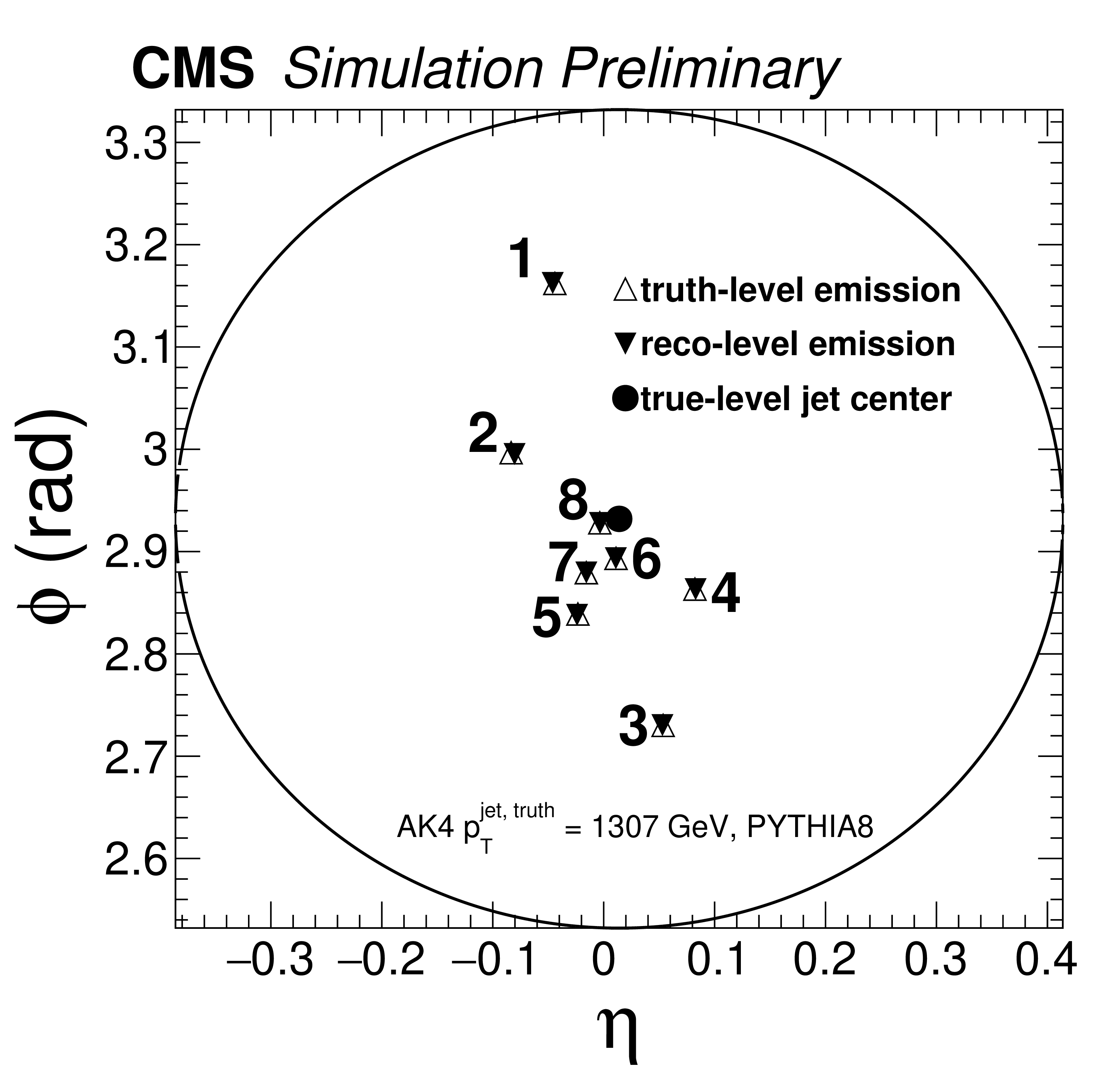
Figure 4:
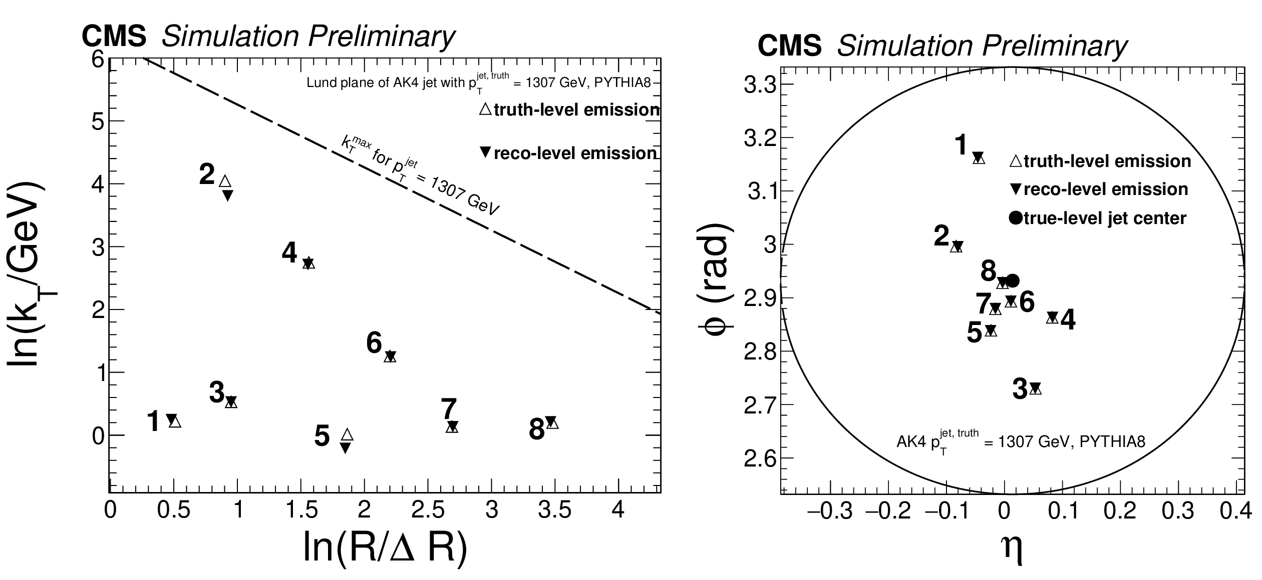
Event displays of a simulated AK4 jet at detector level (solid triangles) and particle level (open triangles). The right-hand side diagram represents the $ \eta $ and $ \phi $ coordinates of the emissions in the CMS coordinate system. The center of the particle-level anti-$ k_{\mathrm{T}} $ jet is represented by the solid circular marker. The circular line with radius $ R = $ 0.4 serves as a proxy for the anti-$ k_{\mathrm{T}} $ distance parameter used to cluster the AK4 jet. The Lund plane on the left panel is associated to the same jet, and is filled with the primary emissions from the CA declustering from left to right (from large angles to small angles). The numbers in both plots represent the order of the emission of the primary CA tree declustering sequence. |
png pdf |
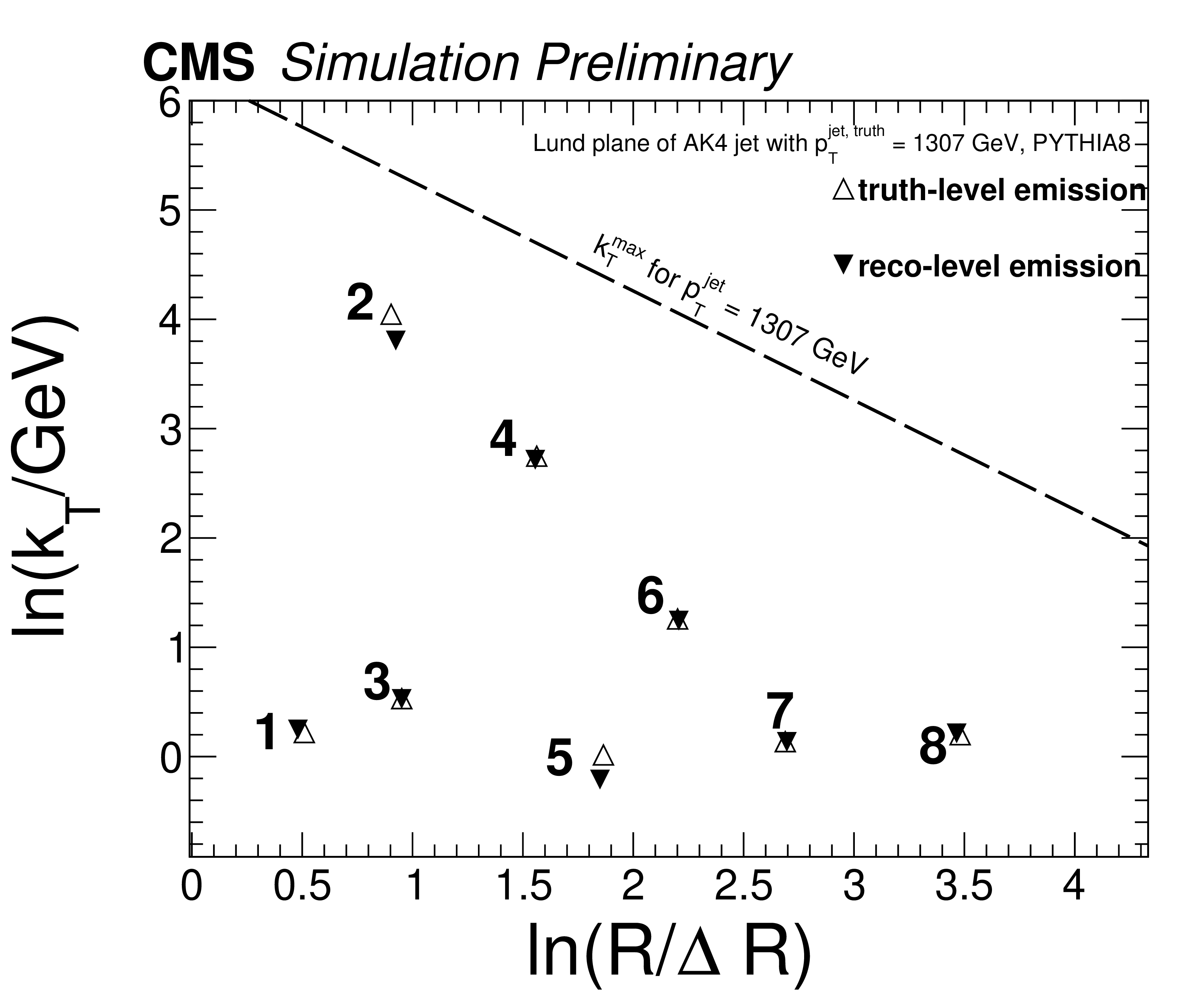
Figure 4-a:
Event displays of a simulated AK4 jet at detector level (solid triangles) and particle level (open triangles). The right-hand side diagram represents the $ \eta $ and $ \phi $ coordinates of the emissions in the CMS coordinate system. The center of the particle-level anti-$ k_{\mathrm{T}} $ jet is represented by the solid circular marker. The circular line with radius $ R = $ 0.4 serves as a proxy for the anti-$ k_{\mathrm{T}} $ distance parameter used to cluster the AK4 jet. The Lund plane on the left panel is associated to the same jet, and is filled with the primary emissions from the CA declustering from left to right (from large angles to small angles). The numbers in both plots represent the order of the emission of the primary CA tree declustering sequence. |
png pdf |
Figure 4-b:
Event displays of a simulated AK4 jet at detector level (solid triangles) and particle level (open triangles). The right-hand side diagram represents the $ \eta $ and $ \phi $ coordinates of the emissions in the CMS coordinate system. The center of the particle-level anti-$ k_{\mathrm{T}} $ jet is represented by the solid circular marker. The circular line with radius $ R = $ 0.4 serves as a proxy for the anti-$ k_{\mathrm{T}} $ distance parameter used to cluster the AK4 jet. The Lund plane on the left panel is associated to the same jet, and is filled with the primary emissions from the CA declustering from left to right (from large angles to small angles). The numbers in both plots represent the order of the emission of the primary CA tree declustering sequence. |
png pdf |
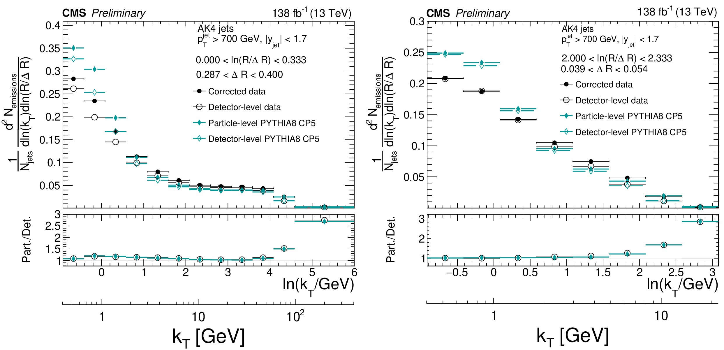
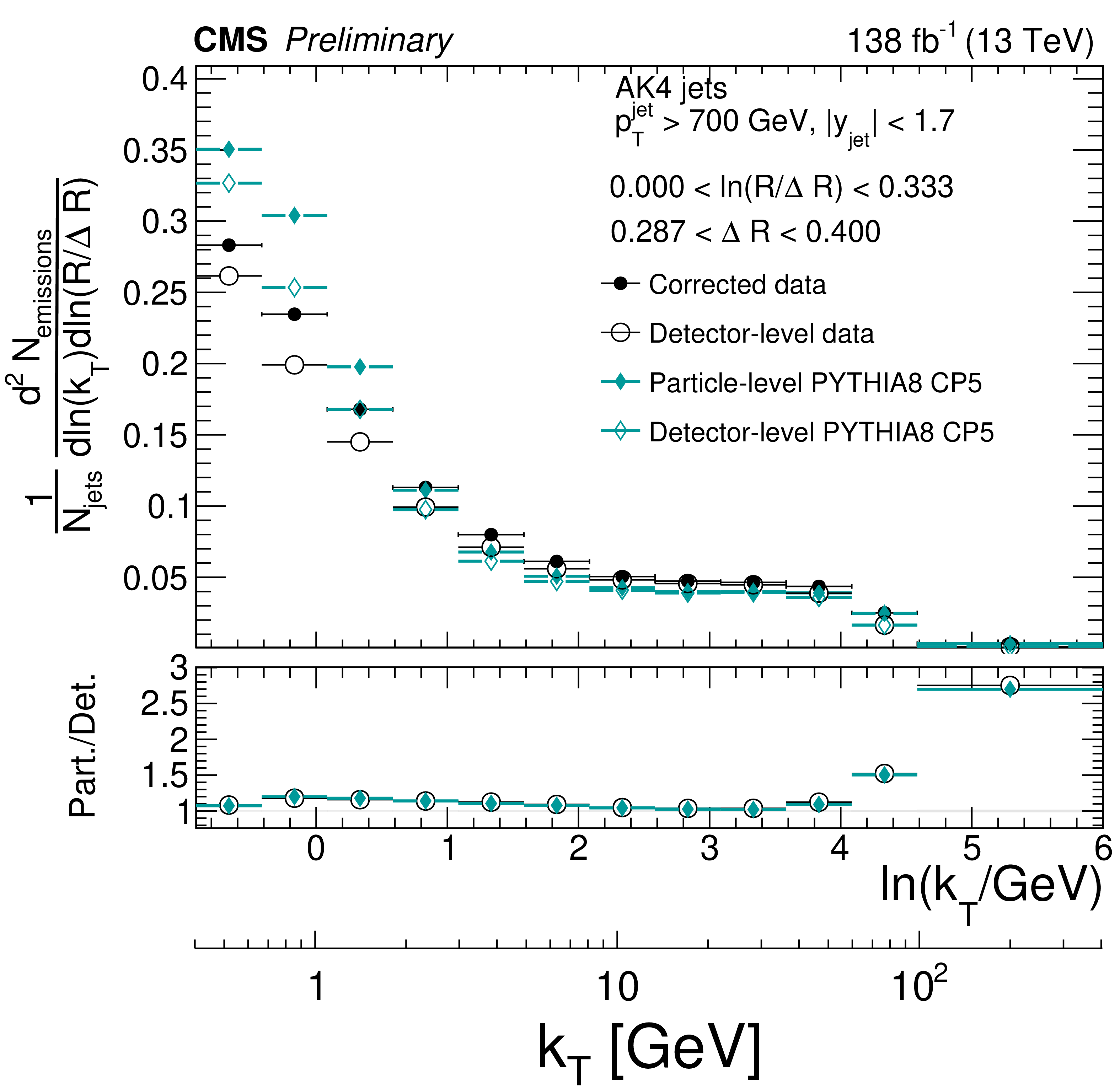
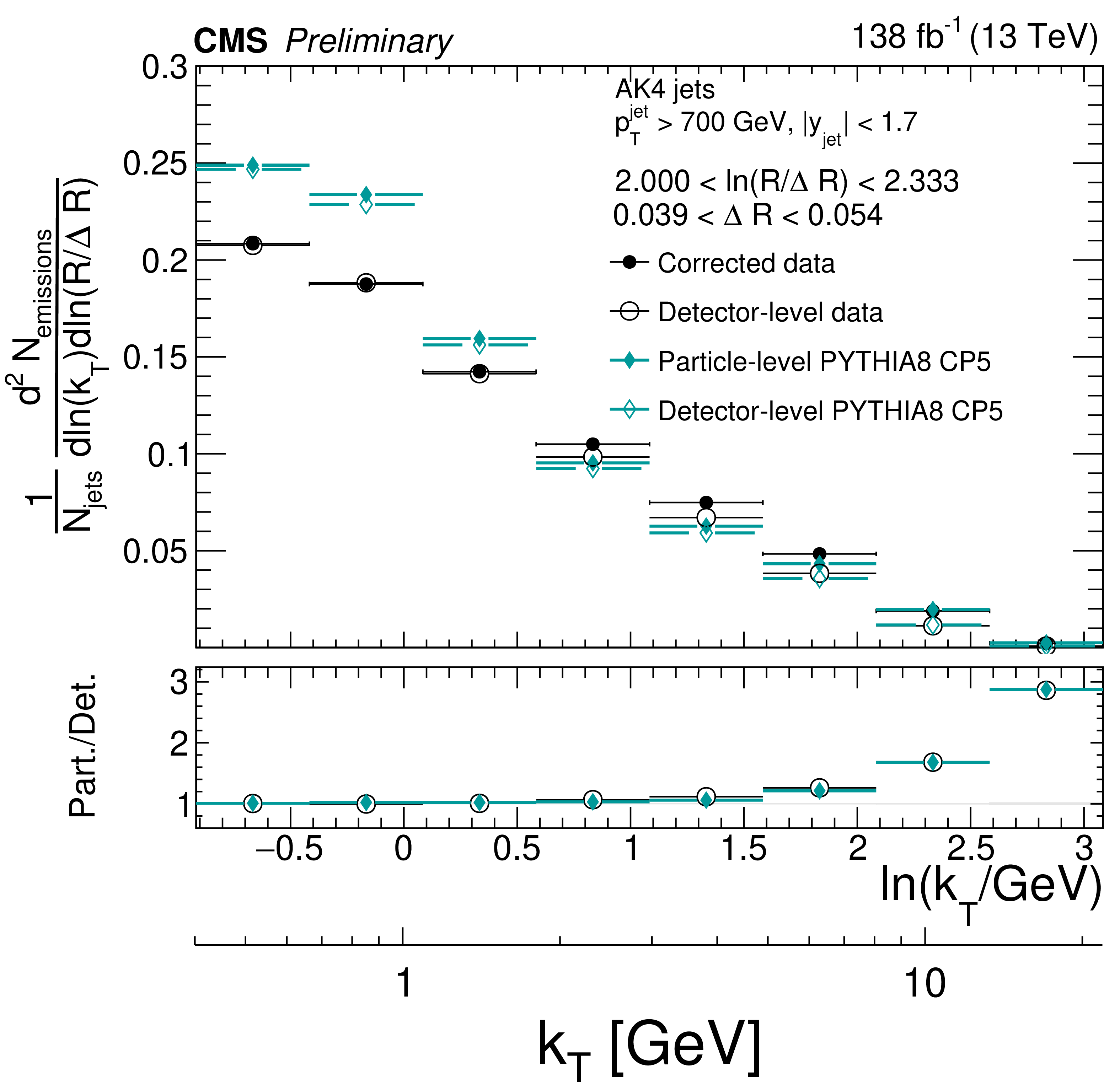
Figure 5:
Detector-level (open symbols) and particle-level (closed symbols) distributions for the data and Monte Carlo simulated events of PYTHIA8 CP5. Only statistical uncertainties are included in this plot. The lower panels show the ratio of the particle-level distributions relative to the respective detector-level distribution, which is used as a metric for the effective modifications of the Lund jet plane density due to the defector effects. The size of the corrections can be inferred from the ratio of the particle-level distributions to the detector-level distributions. |
png pdf |
Figure 5-a:
Detector-level (open symbols) and particle-level (closed symbols) distributions for the data and Monte Carlo simulated events of PYTHIA8 CP5. Only statistical uncertainties are included in this plot. The lower panels show the ratio of the particle-level distributions relative to the respective detector-level distribution, which is used as a metric for the effective modifications of the Lund jet plane density due to the defector effects. The size of the corrections can be inferred from the ratio of the particle-level distributions to the detector-level distributions. |
png pdf |
Figure 5-b:
Detector-level (open symbols) and particle-level (closed symbols) distributions for the data and Monte Carlo simulated events of PYTHIA8 CP5. Only statistical uncertainties are included in this plot. The lower panels show the ratio of the particle-level distributions relative to the respective detector-level distribution, which is used as a metric for the effective modifications of the Lund jet plane density due to the defector effects. The size of the corrections can be inferred from the ratio of the particle-level distributions to the detector-level distributions. |
png pdf |
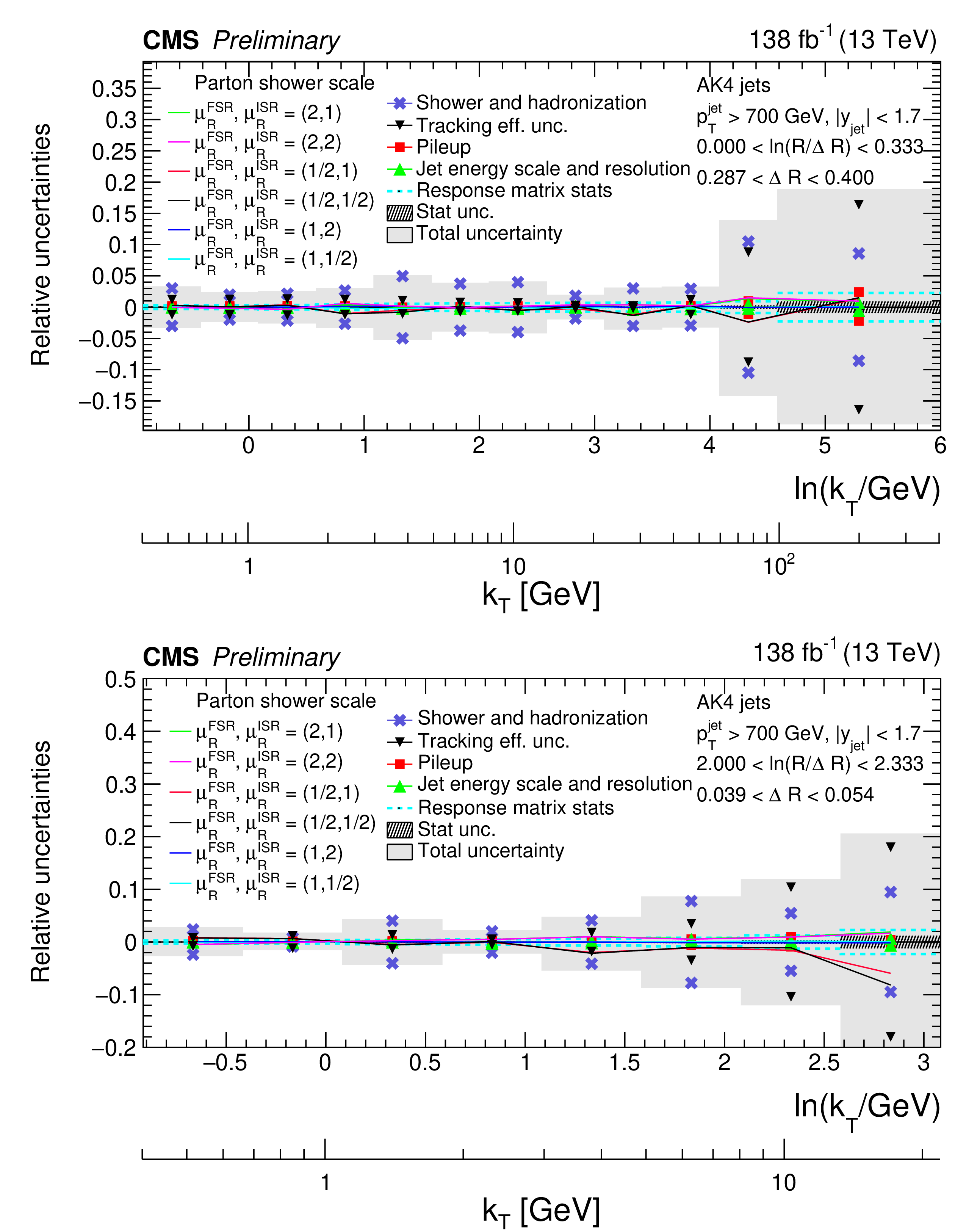
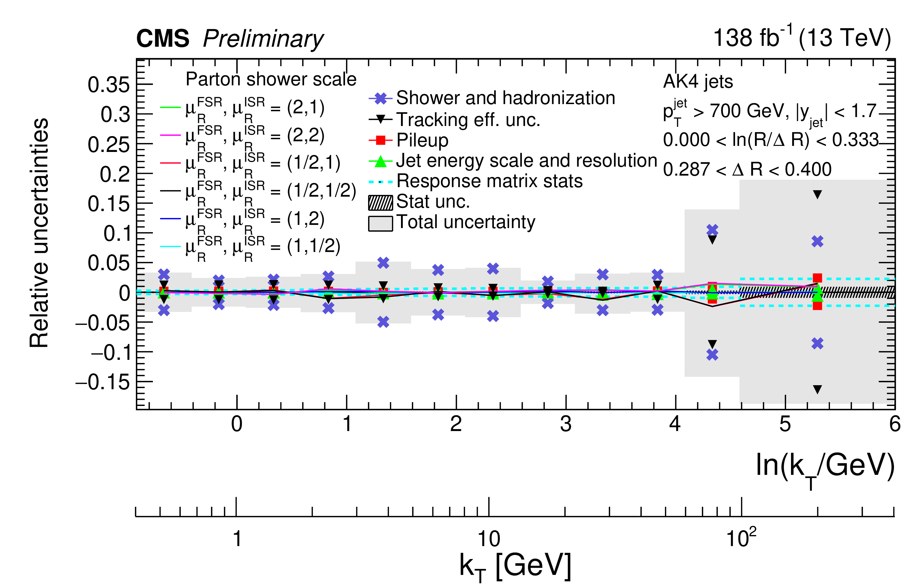
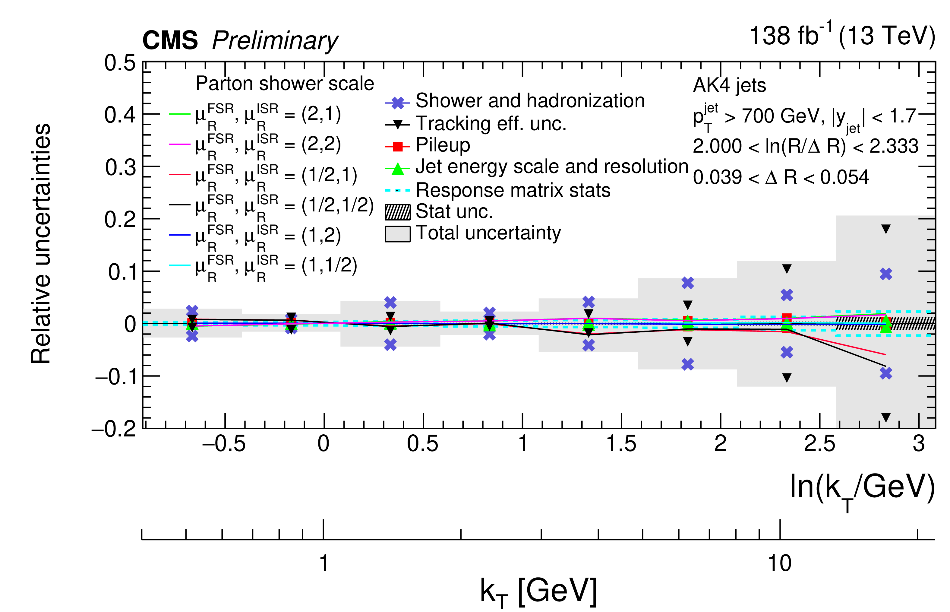
Figure 6:
Different components of the systematic uncertainties for AK4 jets for different slices of the Lund jet plane density. The upper panel is for large angles, while the lower panel is for small angles. The total experimental uncertainty is represented by the filled area. The statistical uncertainties are represented by the hashed band. |
png pdf |
Figure 6-a:
Different components of the systematic uncertainties for AK4 jets for different slices of the Lund jet plane density. The upper panel is for large angles, while the lower panel is for small angles. The total experimental uncertainty is represented by the filled area. The statistical uncertainties are represented by the hashed band. |
png pdf |
Figure 6-b:
Different components of the systematic uncertainties for AK4 jets for different slices of the Lund jet plane density. The upper panel is for large angles, while the lower panel is for small angles. The total experimental uncertainty is represented by the filled area. The statistical uncertainties are represented by the hashed band. |
png pdf |
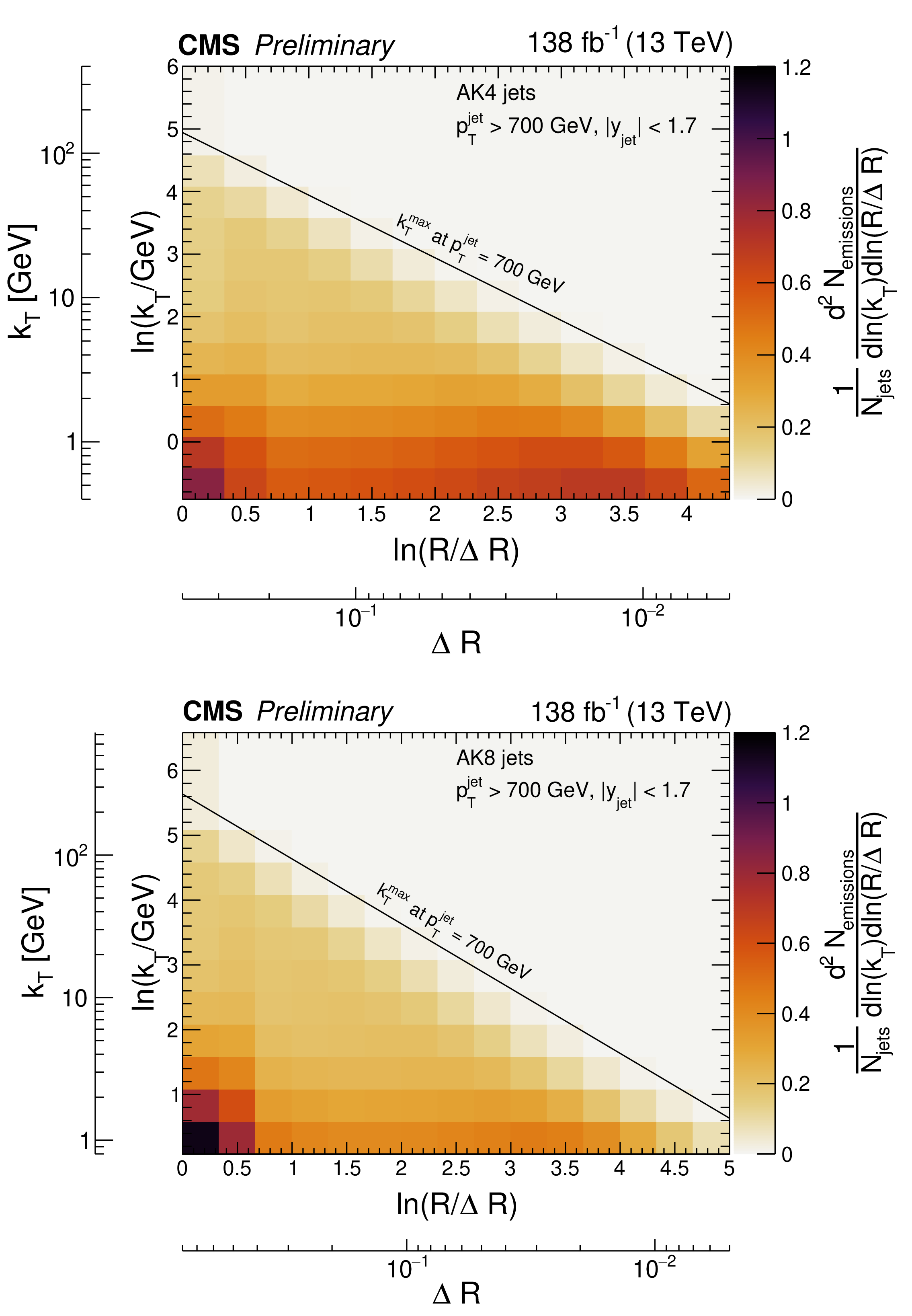
Figure 7:
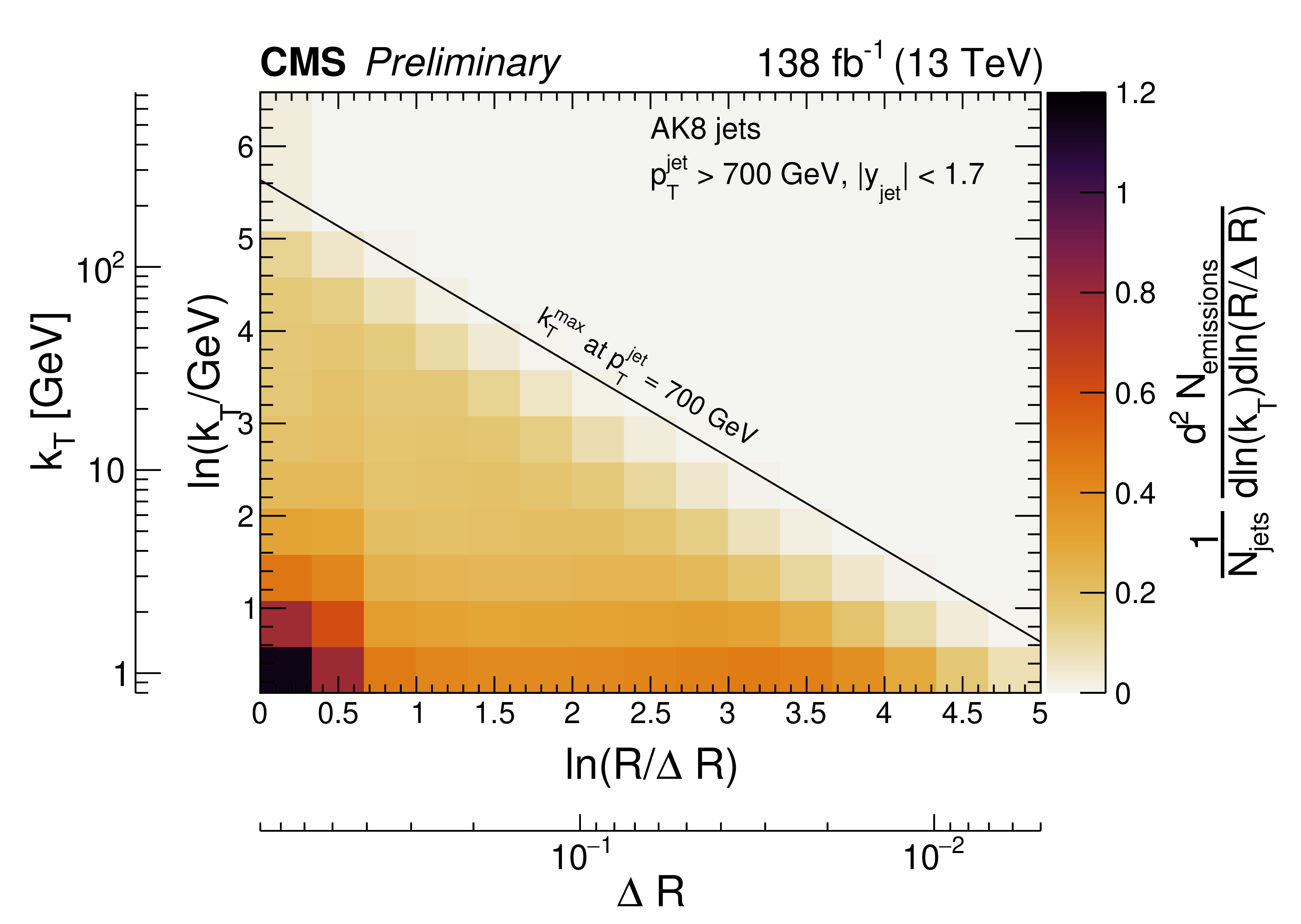
Two-dimensional distributions of the primary Lund jet plane densities corrected to particle level for AK4 jets (upper panel) and AK8 jets (lower panel). The diagonal line in both plots represents the kinematical limit of the emissions for a jet with $ p_{\mathrm{T}}^\text{jet} = $ 700 GeV. |

png pdf |
Figure 7-a:
Two-dimensional distributions of the primary Lund jet plane densities corrected to particle level for AK4 jets (upper panel) and AK8 jets (lower panel). The diagonal line in both plots represents the kinematical limit of the emissions for a jet with $ p_{\mathrm{T}}^\text{jet} = $ 700 GeV. |
png pdf |
Figure 7-b:
Two-dimensional distributions of the primary Lund jet plane densities corrected to particle level for AK4 jets (upper panel) and AK8 jets (lower panel). The diagonal line in both plots represents the kinematical limit of the emissions for a jet with $ p_{\mathrm{T}}^\text{jet} = $ 700 GeV. |
png pdf |
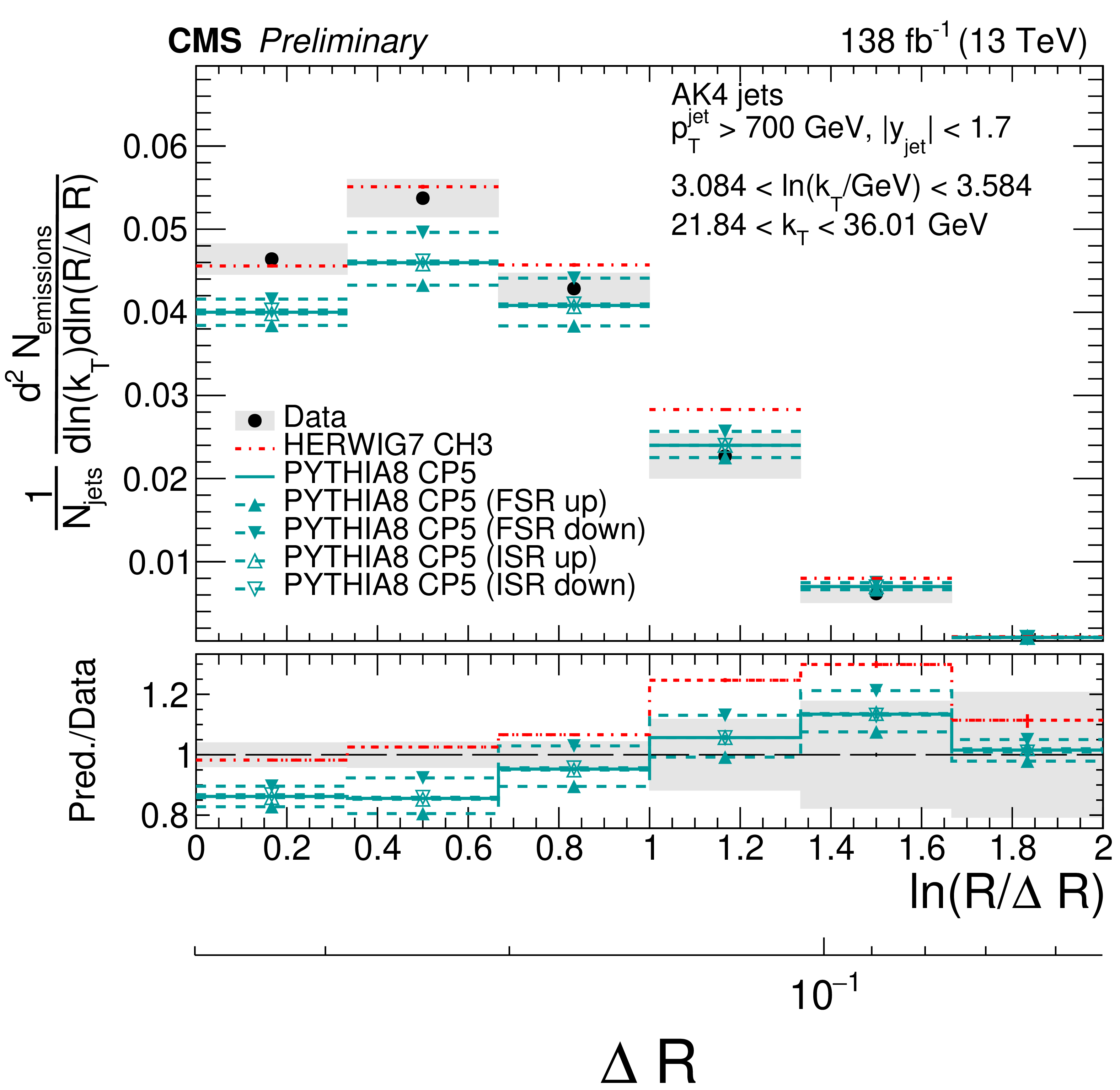
Figure 8:
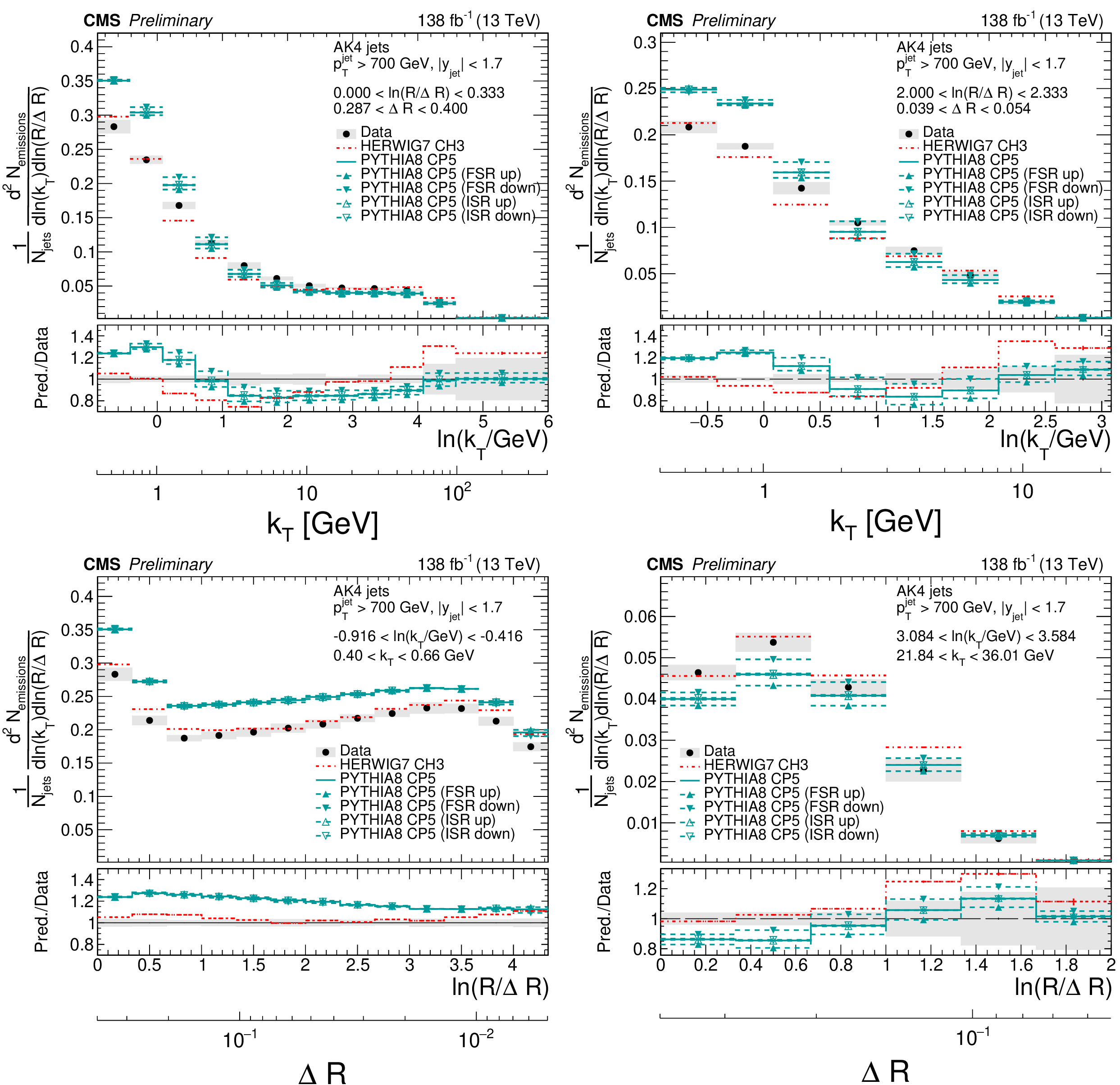
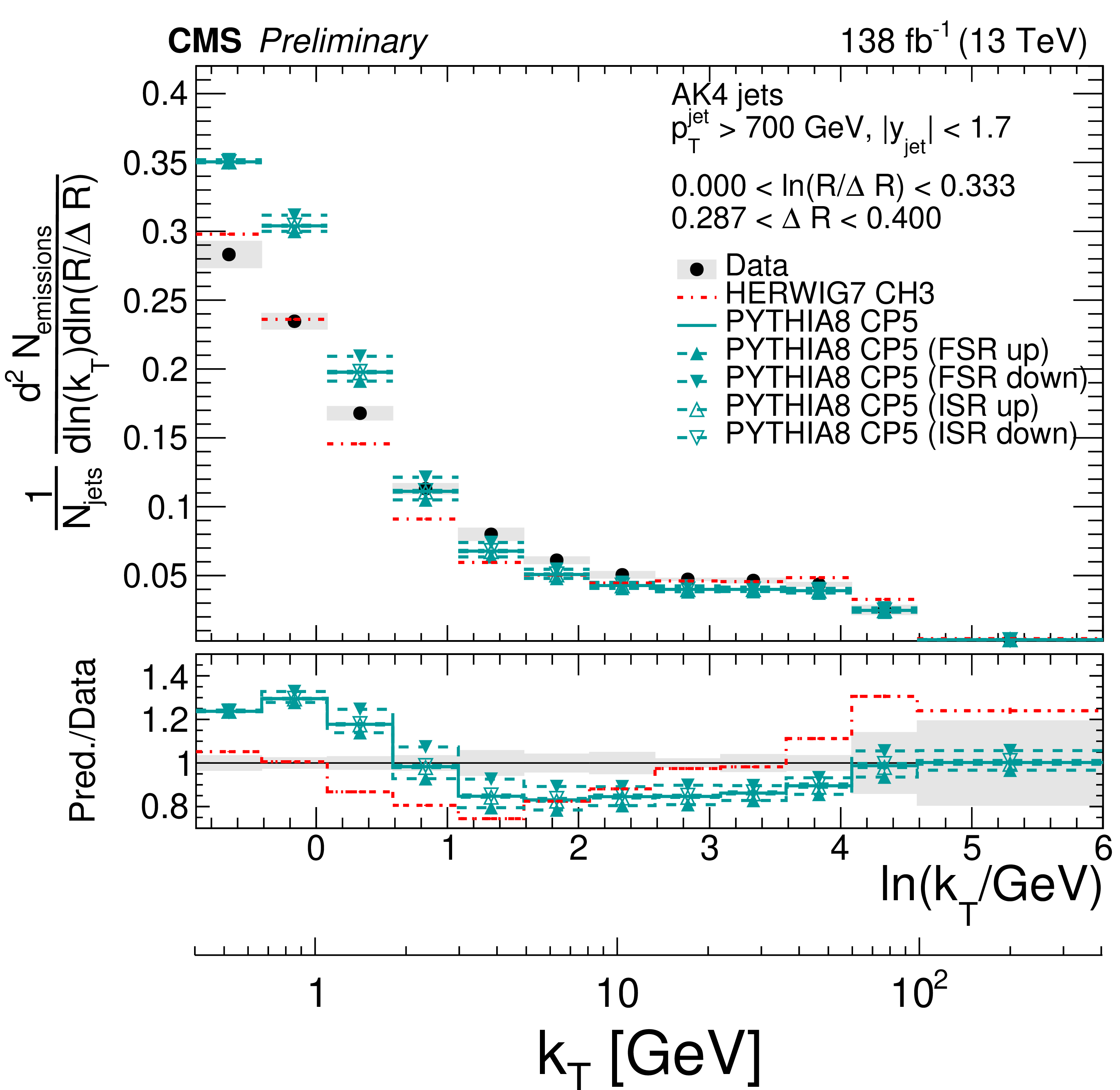
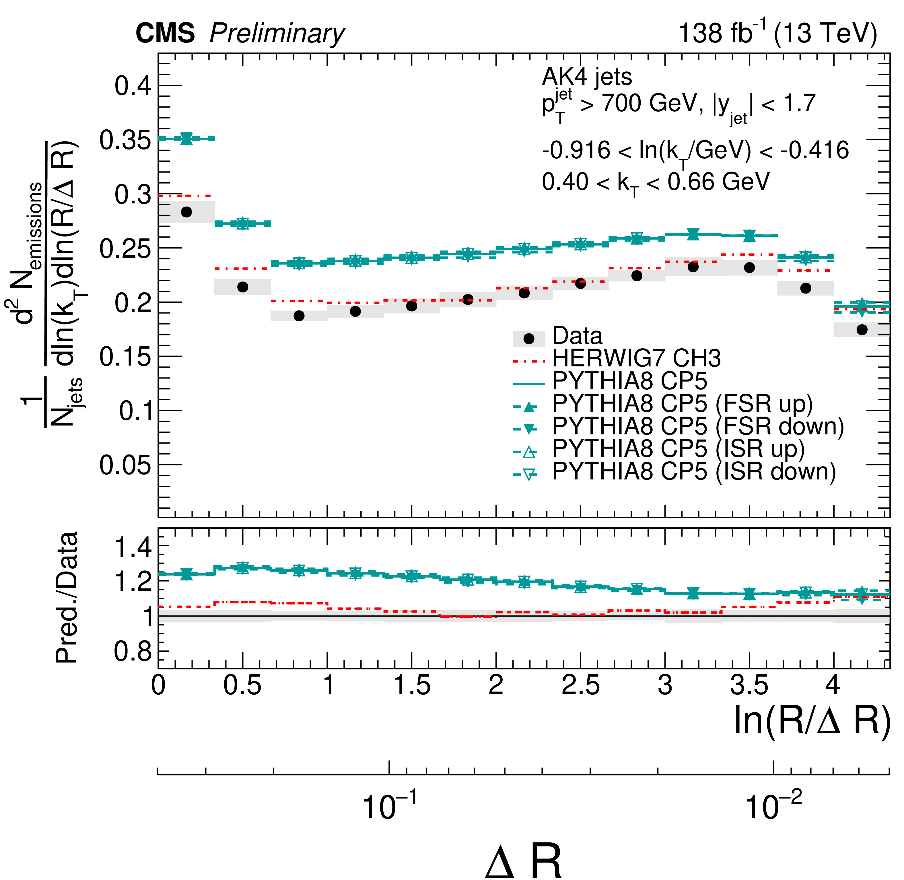
Four slices of the primary Lund jet plane density of AK4 jets compared to predictions by PYTHIA8 CP5 and HERWIG 7 CH3. Variations of the ISR and FSR scales for PYTHIA8 CP5 predictions are shown as well. The band represents the total experimental uncertainty. The upper two panels correspond to vertical slices for fixed $ \ln(R/\Delta R) $ (large angles on upper left, small angles on upper right). The lower two panels correspond to two different horizontal slices for fixed $ \ln(k_{\mathrm{T}}/\,\text{GeV}) $: the lower left panel contains low $ k_{\mathrm{T}} $ splittings, whereas the lower right panel contains high-$ k_{\mathrm{T}} $ splittings, which populate mostly wide-angle radiation. |
png pdf |
Figure 8-a:
Four slices of the primary Lund jet plane density of AK4 jets compared to predictions by PYTHIA8 CP5 and HERWIG 7 CH3. Variations of the ISR and FSR scales for PYTHIA8 CP5 predictions are shown as well. The band represents the total experimental uncertainty. The upper two panels correspond to vertical slices for fixed $ \ln(R/\Delta R) $ (large angles on upper left, small angles on upper right). The lower two panels correspond to two different horizontal slices for fixed $ \ln(k_{\mathrm{T}}/\,\text{GeV}) $: the lower left panel contains low $ k_{\mathrm{T}} $ splittings, whereas the lower right panel contains high-$ k_{\mathrm{T}} $ splittings, which populate mostly wide-angle radiation. |

png pdf |
Figure 8-b:
Four slices of the primary Lund jet plane density of AK4 jets compared to predictions by PYTHIA8 CP5 and HERWIG 7 CH3. Variations of the ISR and FSR scales for PYTHIA8 CP5 predictions are shown as well. The band represents the total experimental uncertainty. The upper two panels correspond to vertical slices for fixed $ \ln(R/\Delta R) $ (large angles on upper left, small angles on upper right). The lower two panels correspond to two different horizontal slices for fixed $ \ln(k_{\mathrm{T}}/\,\text{GeV}) $: the lower left panel contains low $ k_{\mathrm{T}} $ splittings, whereas the lower right panel contains high-$ k_{\mathrm{T}} $ splittings, which populate mostly wide-angle radiation. |
png pdf |
Figure 8-c:
Four slices of the primary Lund jet plane density of AK4 jets compared to predictions by PYTHIA8 CP5 and HERWIG 7 CH3. Variations of the ISR and FSR scales for PYTHIA8 CP5 predictions are shown as well. The band represents the total experimental uncertainty. The upper two panels correspond to vertical slices for fixed $ \ln(R/\Delta R) $ (large angles on upper left, small angles on upper right). The lower two panels correspond to two different horizontal slices for fixed $ \ln(k_{\mathrm{T}}/\,\text{GeV}) $: the lower left panel contains low $ k_{\mathrm{T}} $ splittings, whereas the lower right panel contains high-$ k_{\mathrm{T}} $ splittings, which populate mostly wide-angle radiation. |
png pdf |
Figure 8-d:
Four slices of the primary Lund jet plane density of AK4 jets compared to predictions by PYTHIA8 CP5 and HERWIG 7 CH3. Variations of the ISR and FSR scales for PYTHIA8 CP5 predictions are shown as well. The band represents the total experimental uncertainty. The upper two panels correspond to vertical slices for fixed $ \ln(R/\Delta R) $ (large angles on upper left, small angles on upper right). The lower two panels correspond to two different horizontal slices for fixed $ \ln(k_{\mathrm{T}}/\,\text{GeV}) $: the lower left panel contains low $ k_{\mathrm{T}} $ splittings, whereas the lower right panel contains high-$ k_{\mathrm{T}} $ splittings, which populate mostly wide-angle radiation. |

png pdf |
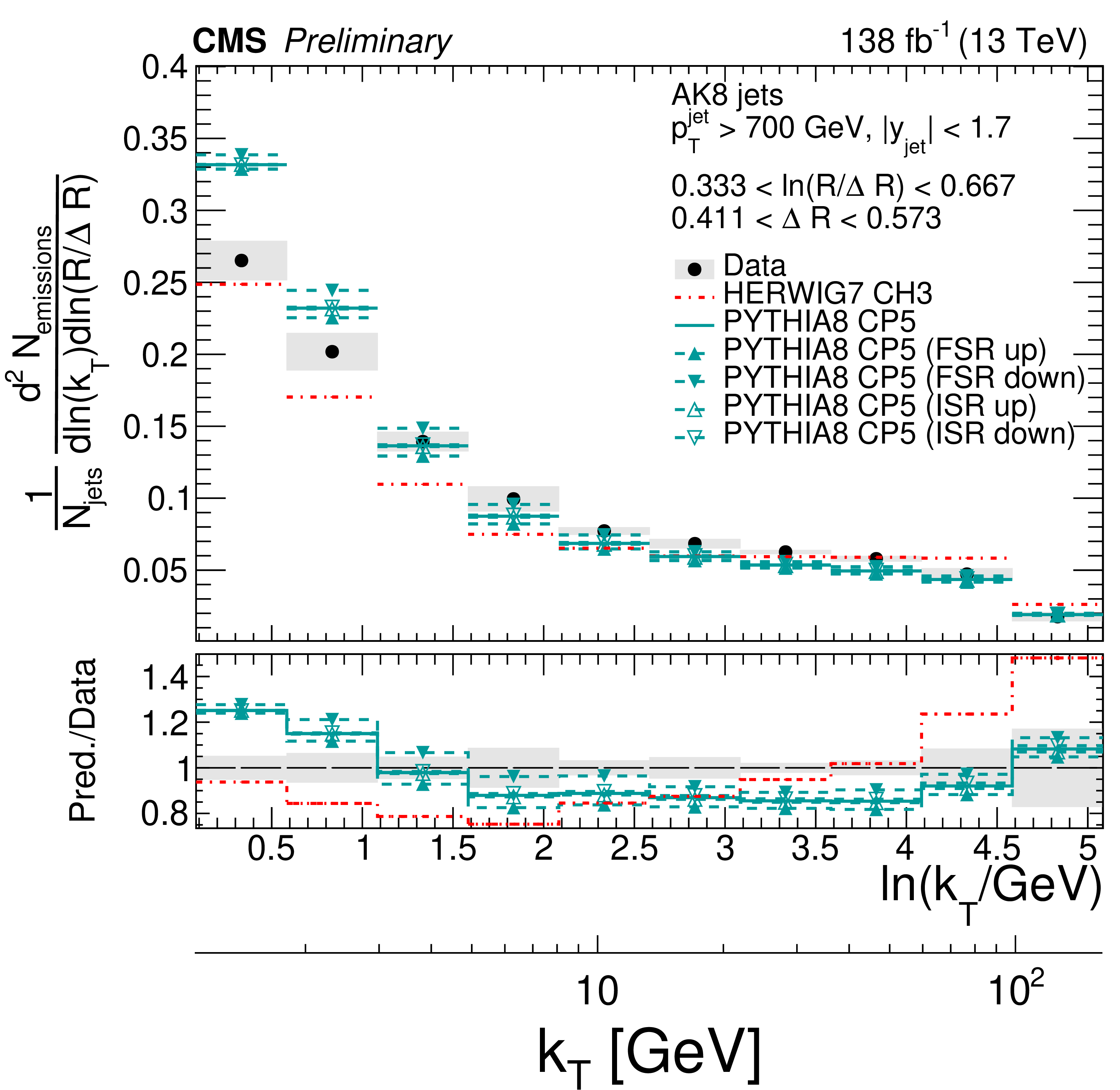
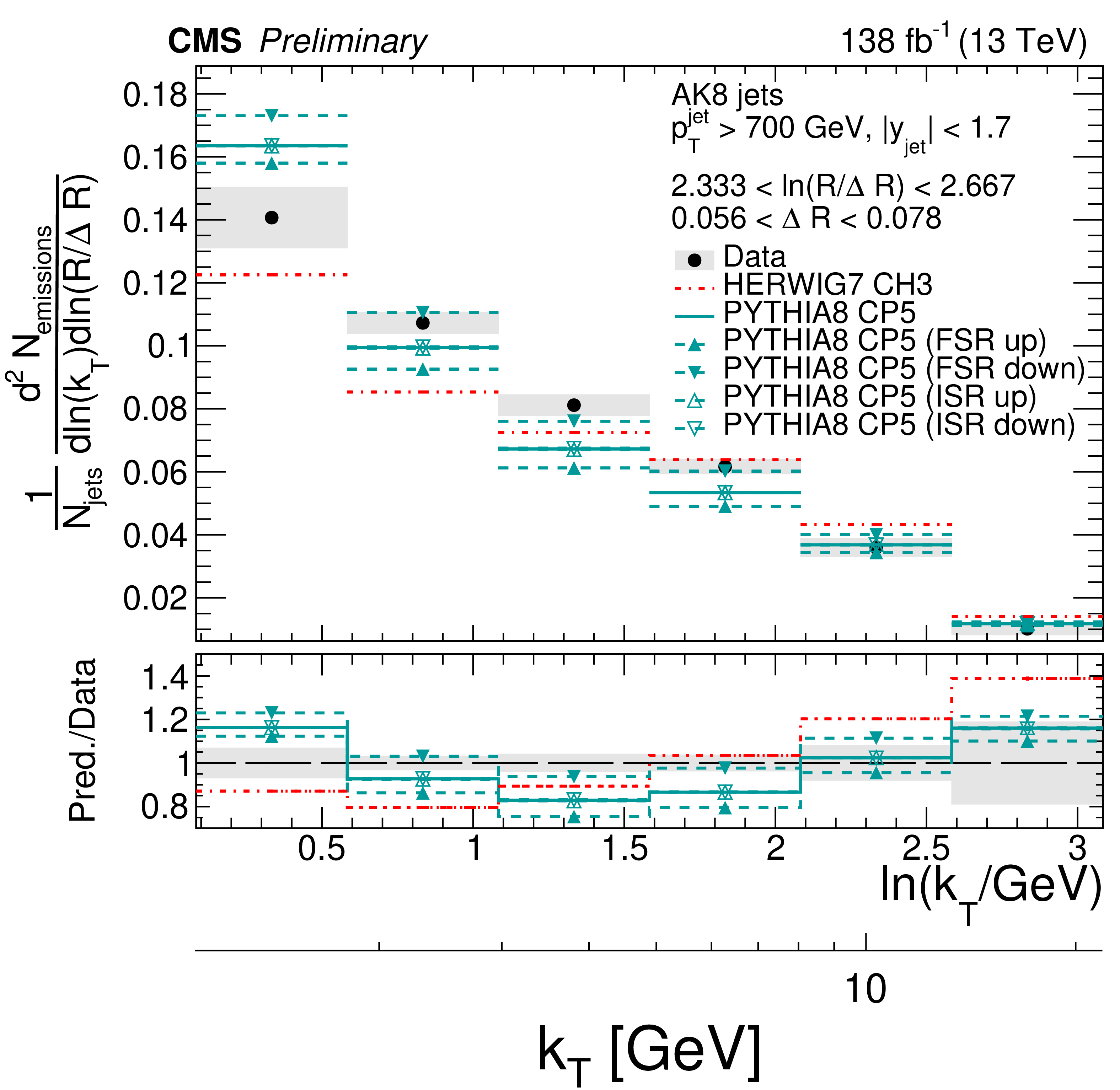
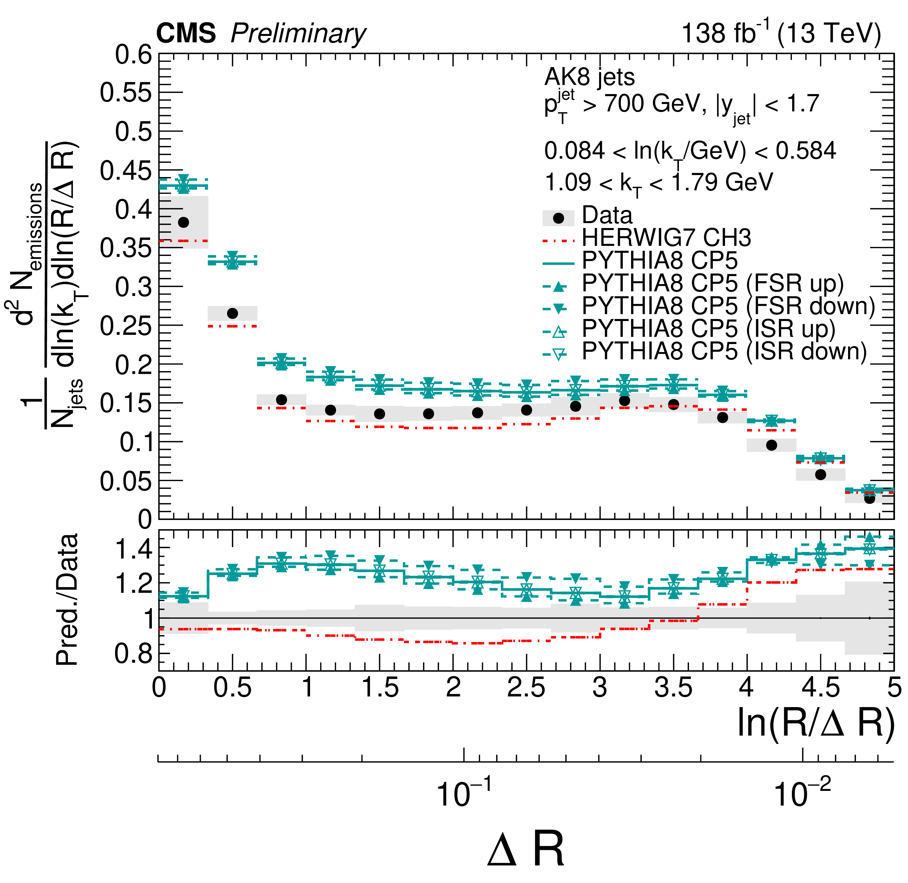
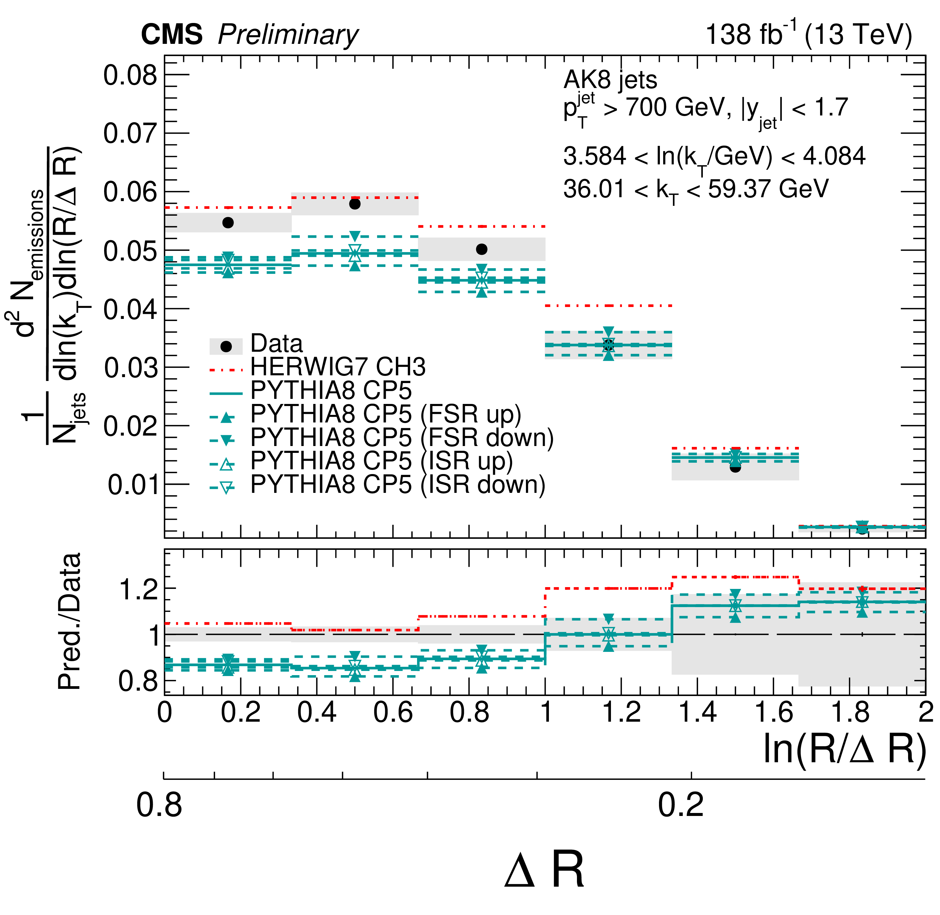
Figure 9:
Four slices of the primary Lund jet plane density of AK8 jets compared to predictions by PYTHIA8 CP5 and HERWIG 7 CH3. Variations of the ISR and FSR scales for PYTHIA8 CP5 predictions are shown as well. The band represents the total experimental uncertainty. The upper two panels correspond to vertical slices for fixed $ \ln(R/\Delta R) $ (large angles on upper left, small angles on upper right). The lower two panels correspond to two different horizontal slices for fixed $ \ln(k_{\mathrm{T}}/\,\text{GeV}) $: the lower left panel corresponds to low $ k_{\mathrm{T}} $ splittings and spans the full range in $ \ln(R/\Delta R) $, whereas the lower right panel corresponds to high-$ k_{\mathrm{T}} $ splittings, which populate mostly wide-angle radiation. |
png pdf |
Figure 9-a:
Four slices of the primary Lund jet plane density of AK8 jets compared to predictions by PYTHIA8 CP5 and HERWIG 7 CH3. Variations of the ISR and FSR scales for PYTHIA8 CP5 predictions are shown as well. The band represents the total experimental uncertainty. The upper two panels correspond to vertical slices for fixed $ \ln(R/\Delta R) $ (large angles on upper left, small angles on upper right). The lower two panels correspond to two different horizontal slices for fixed $ \ln(k_{\mathrm{T}}/\,\text{GeV}) $: the lower left panel corresponds to low $ k_{\mathrm{T}} $ splittings and spans the full range in $ \ln(R/\Delta R) $, whereas the lower right panel corresponds to high-$ k_{\mathrm{T}} $ splittings, which populate mostly wide-angle radiation. |
png pdf |
Figure 9-b:
Four slices of the primary Lund jet plane density of AK8 jets compared to predictions by PYTHIA8 CP5 and HERWIG 7 CH3. Variations of the ISR and FSR scales for PYTHIA8 CP5 predictions are shown as well. The band represents the total experimental uncertainty. The upper two panels correspond to vertical slices for fixed $ \ln(R/\Delta R) $ (large angles on upper left, small angles on upper right). The lower two panels correspond to two different horizontal slices for fixed $ \ln(k_{\mathrm{T}}/\,\text{GeV}) $: the lower left panel corresponds to low $ k_{\mathrm{T}} $ splittings and spans the full range in $ \ln(R/\Delta R) $, whereas the lower right panel corresponds to high-$ k_{\mathrm{T}} $ splittings, which populate mostly wide-angle radiation. |
png pdf |
Figure 9-c:
Four slices of the primary Lund jet plane density of AK8 jets compared to predictions by PYTHIA8 CP5 and HERWIG 7 CH3. Variations of the ISR and FSR scales for PYTHIA8 CP5 predictions are shown as well. The band represents the total experimental uncertainty. The upper two panels correspond to vertical slices for fixed $ \ln(R/\Delta R) $ (large angles on upper left, small angles on upper right). The lower two panels correspond to two different horizontal slices for fixed $ \ln(k_{\mathrm{T}}/\,\text{GeV}) $: the lower left panel corresponds to low $ k_{\mathrm{T}} $ splittings and spans the full range in $ \ln(R/\Delta R) $, whereas the lower right panel corresponds to high-$ k_{\mathrm{T}} $ splittings, which populate mostly wide-angle radiation. |
png pdf |
Figure 9-d:
Four slices of the primary Lund jet plane density of AK8 jets compared to predictions by PYTHIA8 CP5 and HERWIG 7 CH3. Variations of the ISR and FSR scales for PYTHIA8 CP5 predictions are shown as well. The band represents the total experimental uncertainty. The upper two panels correspond to vertical slices for fixed $ \ln(R/\Delta R) $ (large angles on upper left, small angles on upper right). The lower two panels correspond to two different horizontal slices for fixed $ \ln(k_{\mathrm{T}}/\,\text{GeV}) $: the lower left panel corresponds to low $ k_{\mathrm{T}} $ splittings and spans the full range in $ \ln(R/\Delta R) $, whereas the lower right panel corresponds to high-$ k_{\mathrm{T}} $ splittings, which populate mostly wide-angle radiation. |
png pdf |
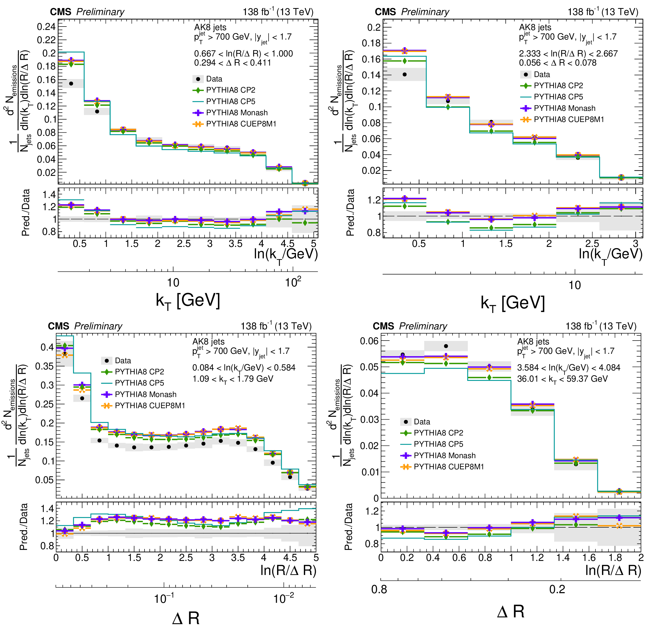
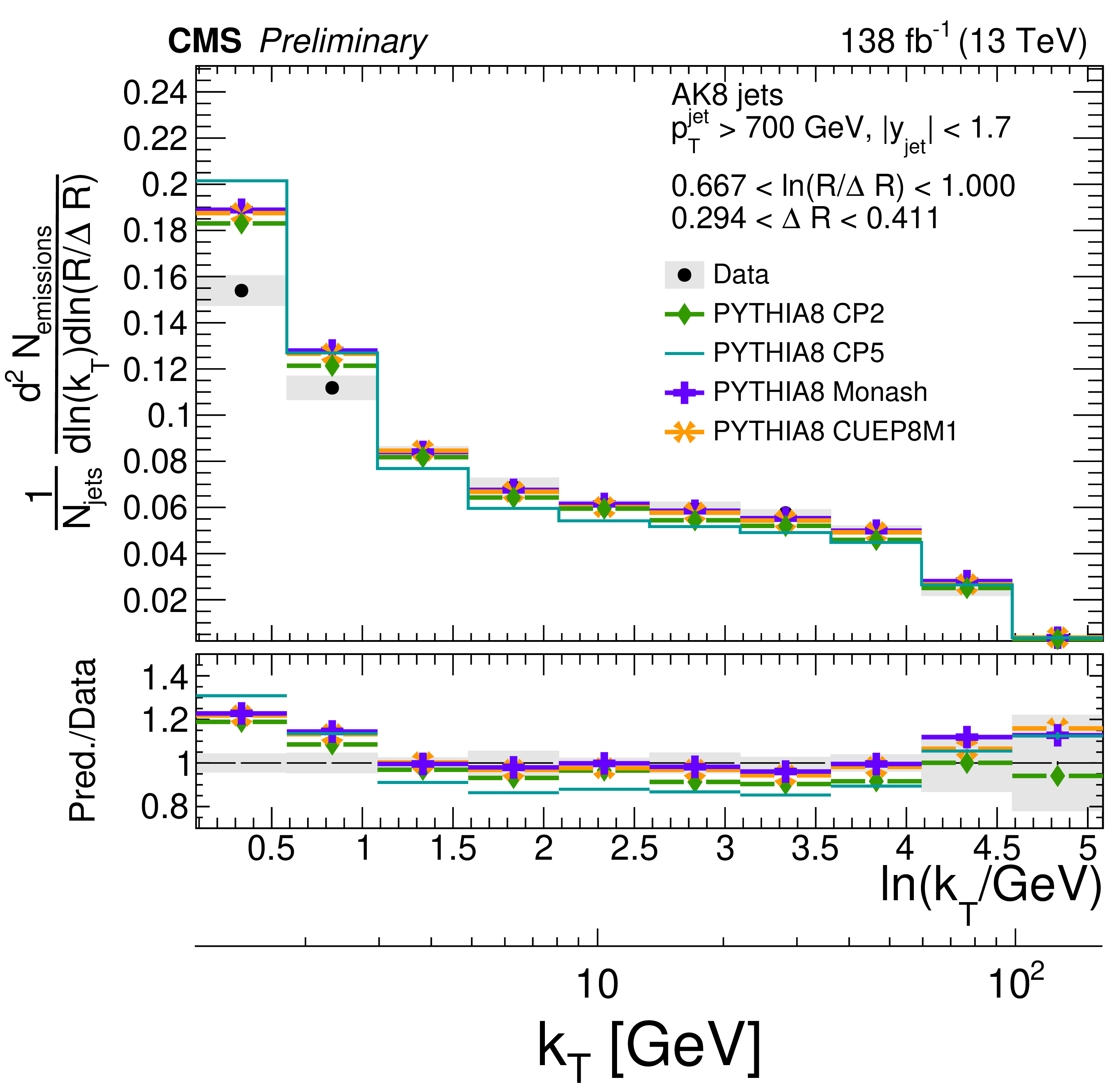
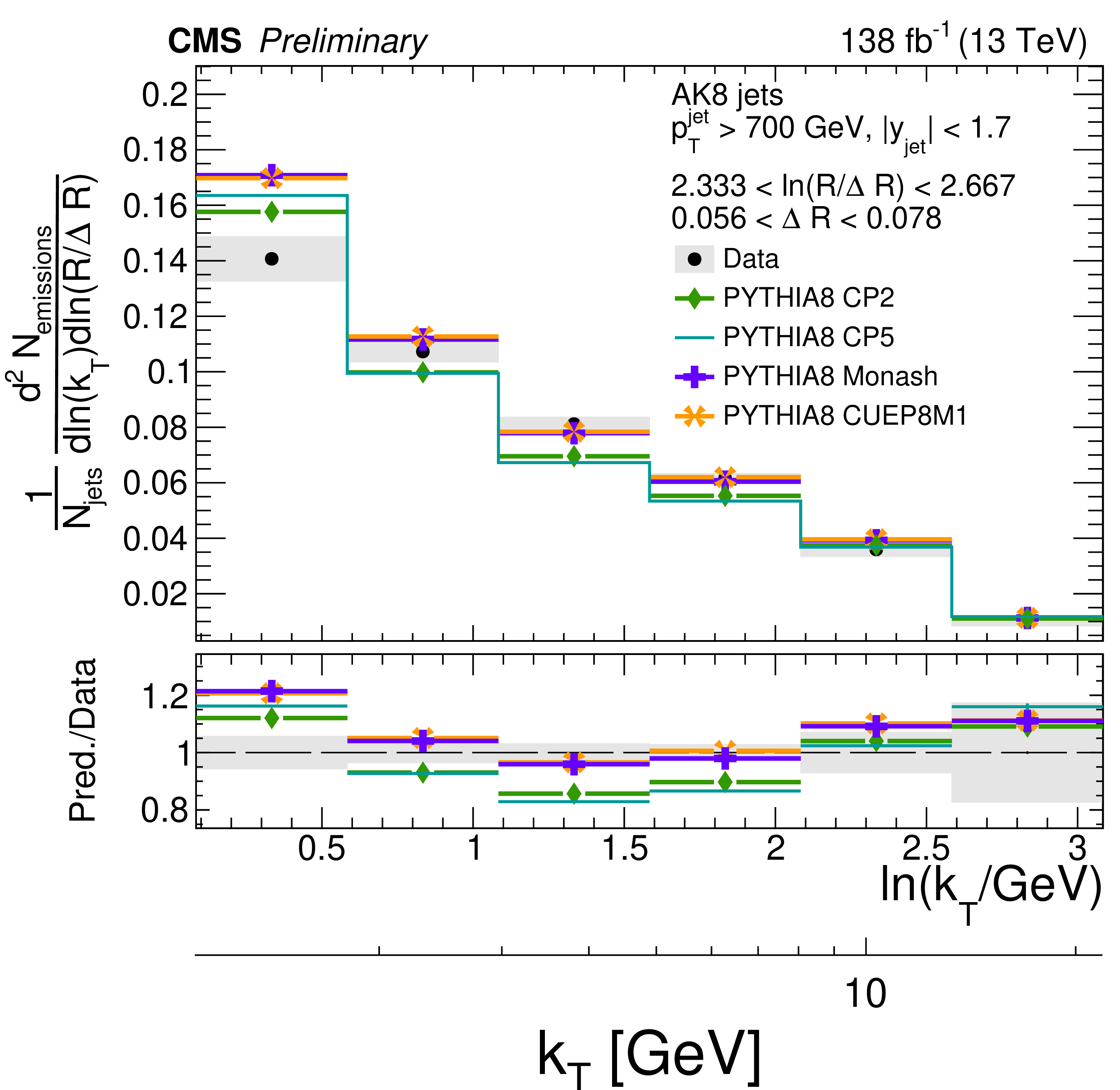
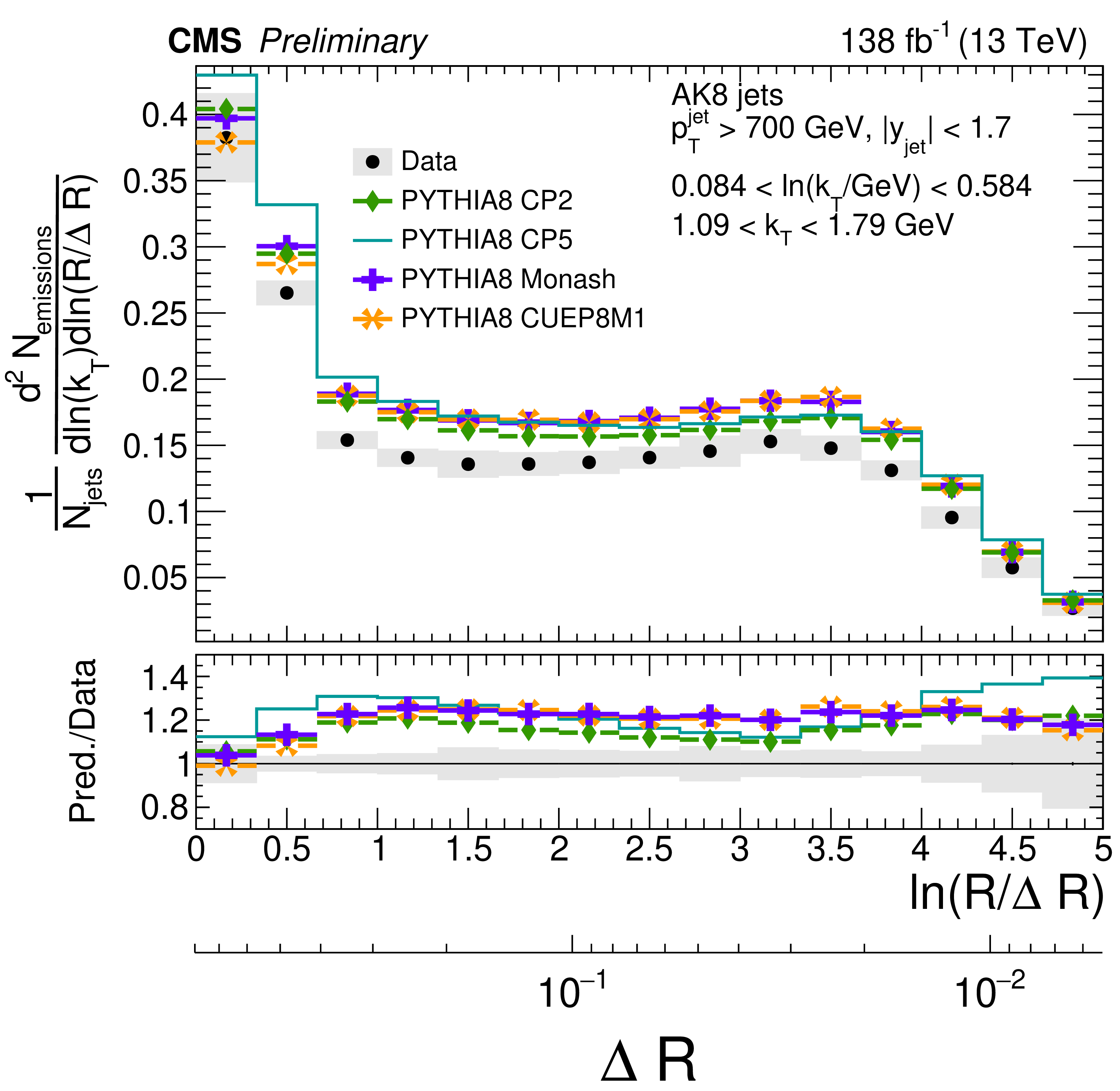
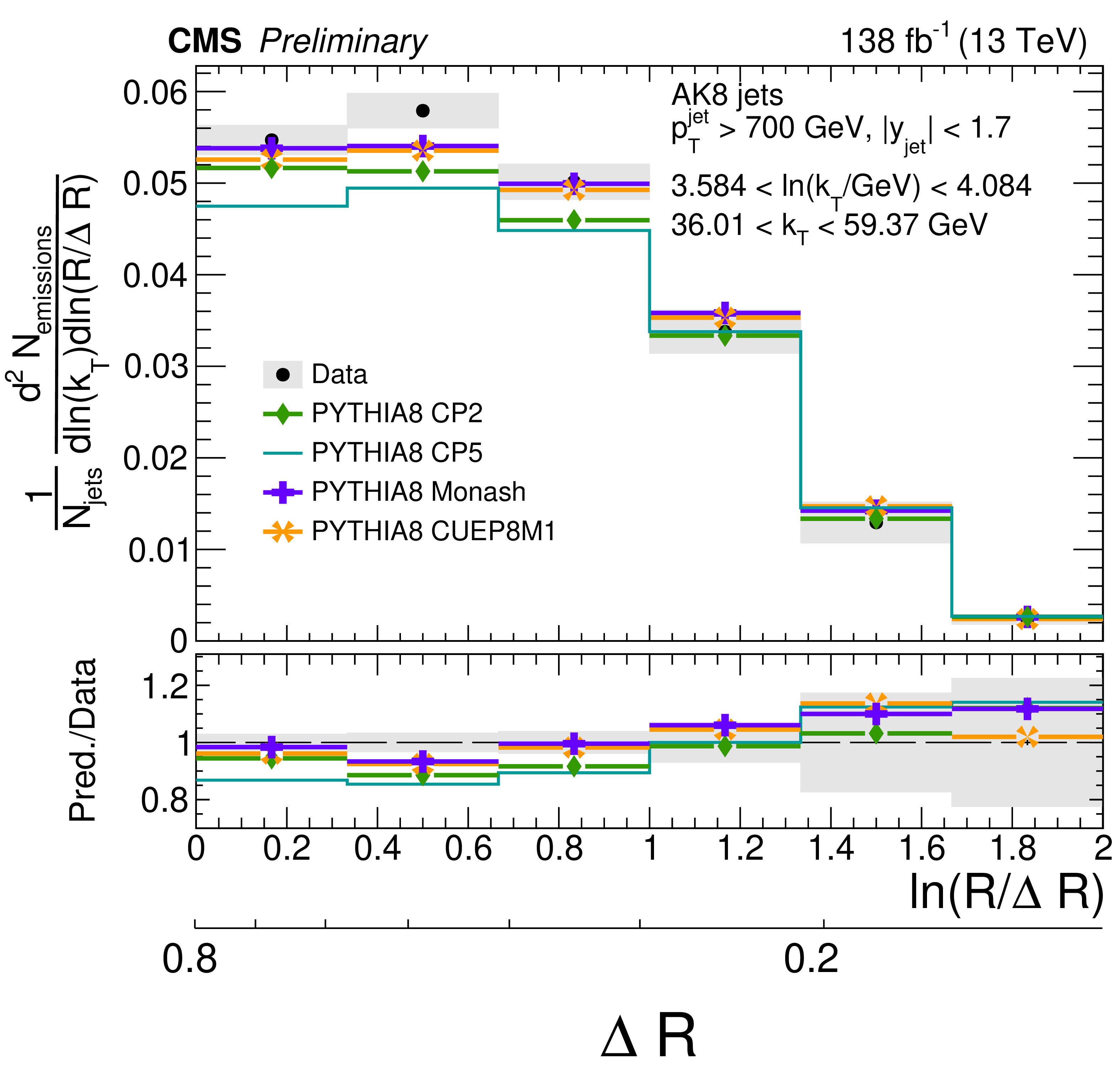
Figure 10:
Four different slices of the primary Lund jet plane density of AK8 jets compared to predictions generated with PYTHIA8 using tunes CP2, CP5, Monash, and CUEP8M1. The band represents the total experimental uncertainty. The upper two panels correspond to vertical slices of the Lund jet plane for fixed $ \ln(R/\Delta R) $ (large angles on upper left, small angles on upper right). The lower two panels correspond to two different horizontal slices for fixed $ \ln(k_{\mathrm{T}}/\,\text{GeV}) $: the lower left panel corresponds to low $ k_{\mathrm{T}} $ splittings and spans the full range in $ \ln(R/\Delta R) $, whereas the lower right panel corresponds to high-$ k_{\mathrm{T}} $ splittings, which populate mostly wide-angle radiation. |
png pdf |
Figure 10-a:
Four different slices of the primary Lund jet plane density of AK8 jets compared to predictions generated with PYTHIA8 using tunes CP2, CP5, Monash, and CUEP8M1. The band represents the total experimental uncertainty. The upper two panels correspond to vertical slices of the Lund jet plane for fixed $ \ln(R/\Delta R) $ (large angles on upper left, small angles on upper right). The lower two panels correspond to two different horizontal slices for fixed $ \ln(k_{\mathrm{T}}/\,\text{GeV}) $: the lower left panel corresponds to low $ k_{\mathrm{T}} $ splittings and spans the full range in $ \ln(R/\Delta R) $, whereas the lower right panel corresponds to high-$ k_{\mathrm{T}} $ splittings, which populate mostly wide-angle radiation. |
png pdf |
Figure 10-b:
Four different slices of the primary Lund jet plane density of AK8 jets compared to predictions generated with PYTHIA8 using tunes CP2, CP5, Monash, and CUEP8M1. The band represents the total experimental uncertainty. The upper two panels correspond to vertical slices of the Lund jet plane for fixed $ \ln(R/\Delta R) $ (large angles on upper left, small angles on upper right). The lower two panels correspond to two different horizontal slices for fixed $ \ln(k_{\mathrm{T}}/\,\text{GeV}) $: the lower left panel corresponds to low $ k_{\mathrm{T}} $ splittings and spans the full range in $ \ln(R/\Delta R) $, whereas the lower right panel corresponds to high-$ k_{\mathrm{T}} $ splittings, which populate mostly wide-angle radiation. |
png pdf |
Figure 10-c:
Four different slices of the primary Lund jet plane density of AK8 jets compared to predictions generated with PYTHIA8 using tunes CP2, CP5, Monash, and CUEP8M1. The band represents the total experimental uncertainty. The upper two panels correspond to vertical slices of the Lund jet plane for fixed $ \ln(R/\Delta R) $ (large angles on upper left, small angles on upper right). The lower two panels correspond to two different horizontal slices for fixed $ \ln(k_{\mathrm{T}}/\,\text{GeV}) $: the lower left panel corresponds to low $ k_{\mathrm{T}} $ splittings and spans the full range in $ \ln(R/\Delta R) $, whereas the lower right panel corresponds to high-$ k_{\mathrm{T}} $ splittings, which populate mostly wide-angle radiation. |
png pdf |
Figure 10-d:
Four different slices of the primary Lund jet plane density of AK8 jets compared to predictions generated with PYTHIA8 using tunes CP2, CP5, Monash, and CUEP8M1. The band represents the total experimental uncertainty. The upper two panels correspond to vertical slices of the Lund jet plane for fixed $ \ln(R/\Delta R) $ (large angles on upper left, small angles on upper right). The lower two panels correspond to two different horizontal slices for fixed $ \ln(k_{\mathrm{T}}/\,\text{GeV}) $: the lower left panel corresponds to low $ k_{\mathrm{T}} $ splittings and spans the full range in $ \ln(R/\Delta R) $, whereas the lower right panel corresponds to high-$ k_{\mathrm{T}} $ splittings, which populate mostly wide-angle radiation. |
png pdf |
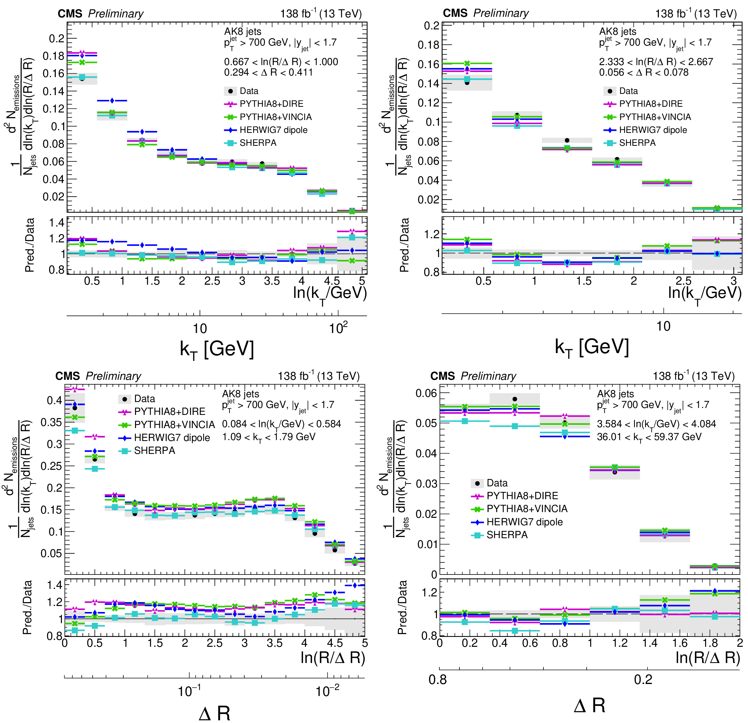
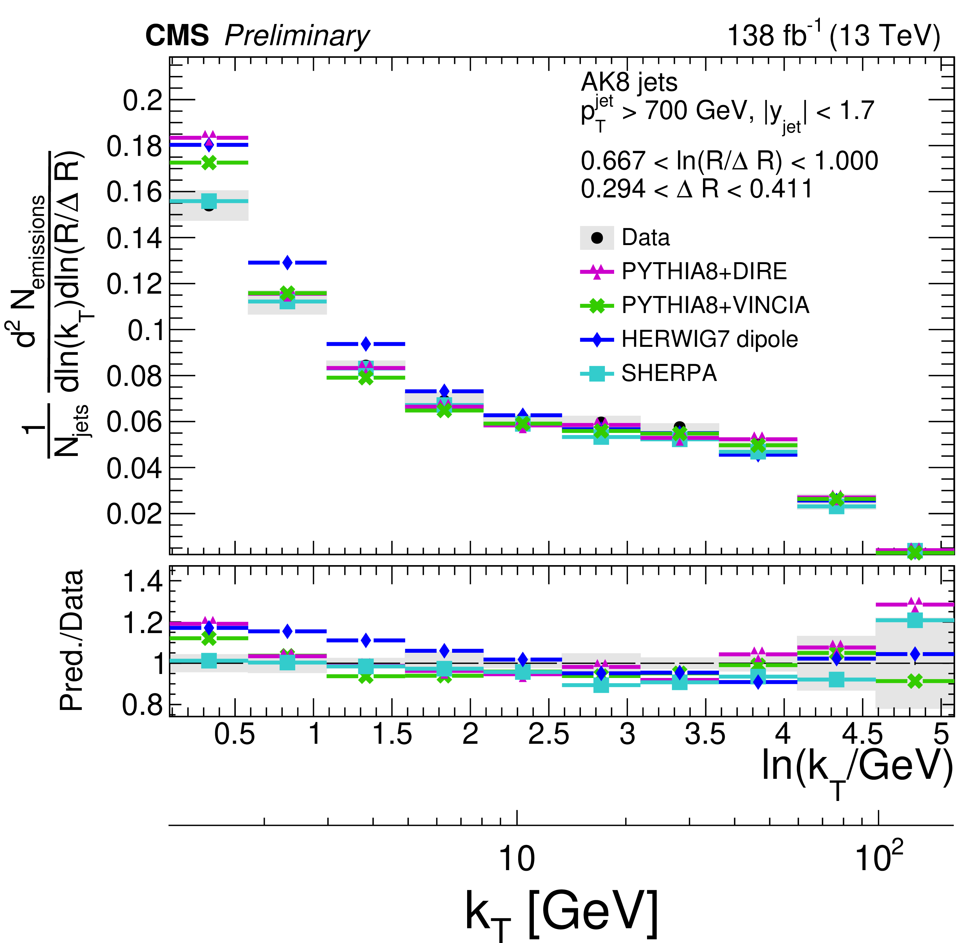
Figure 11:
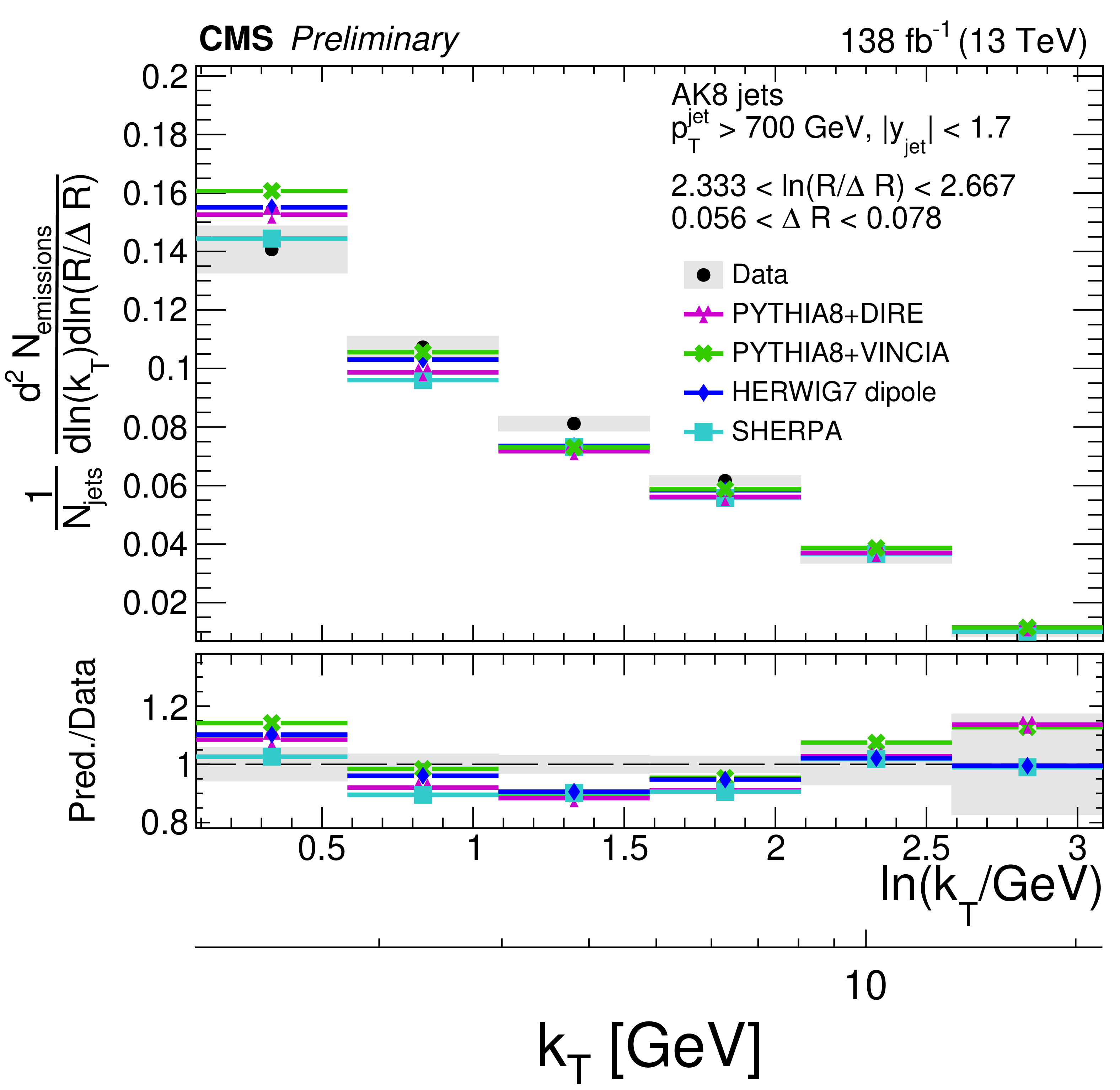
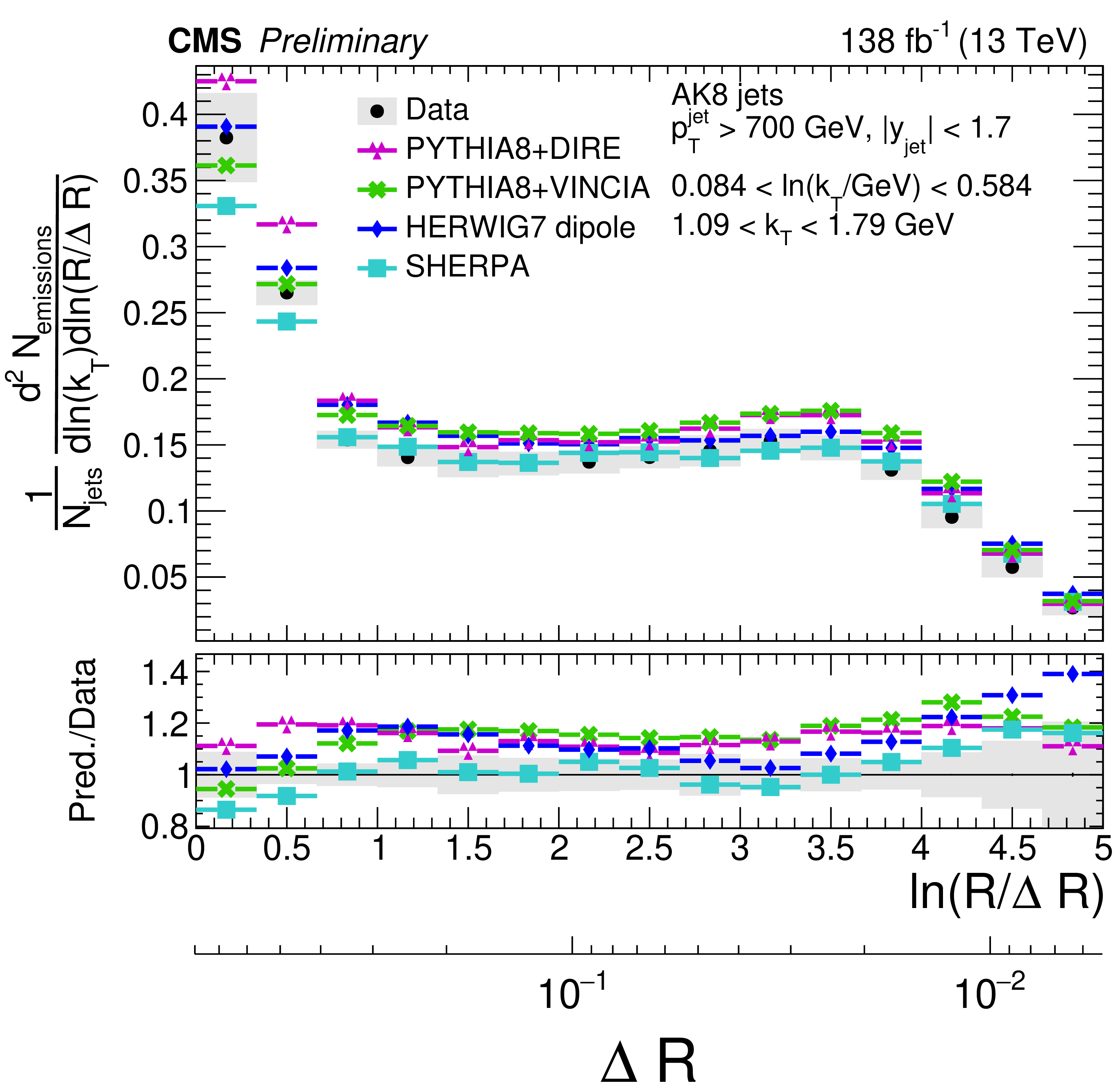
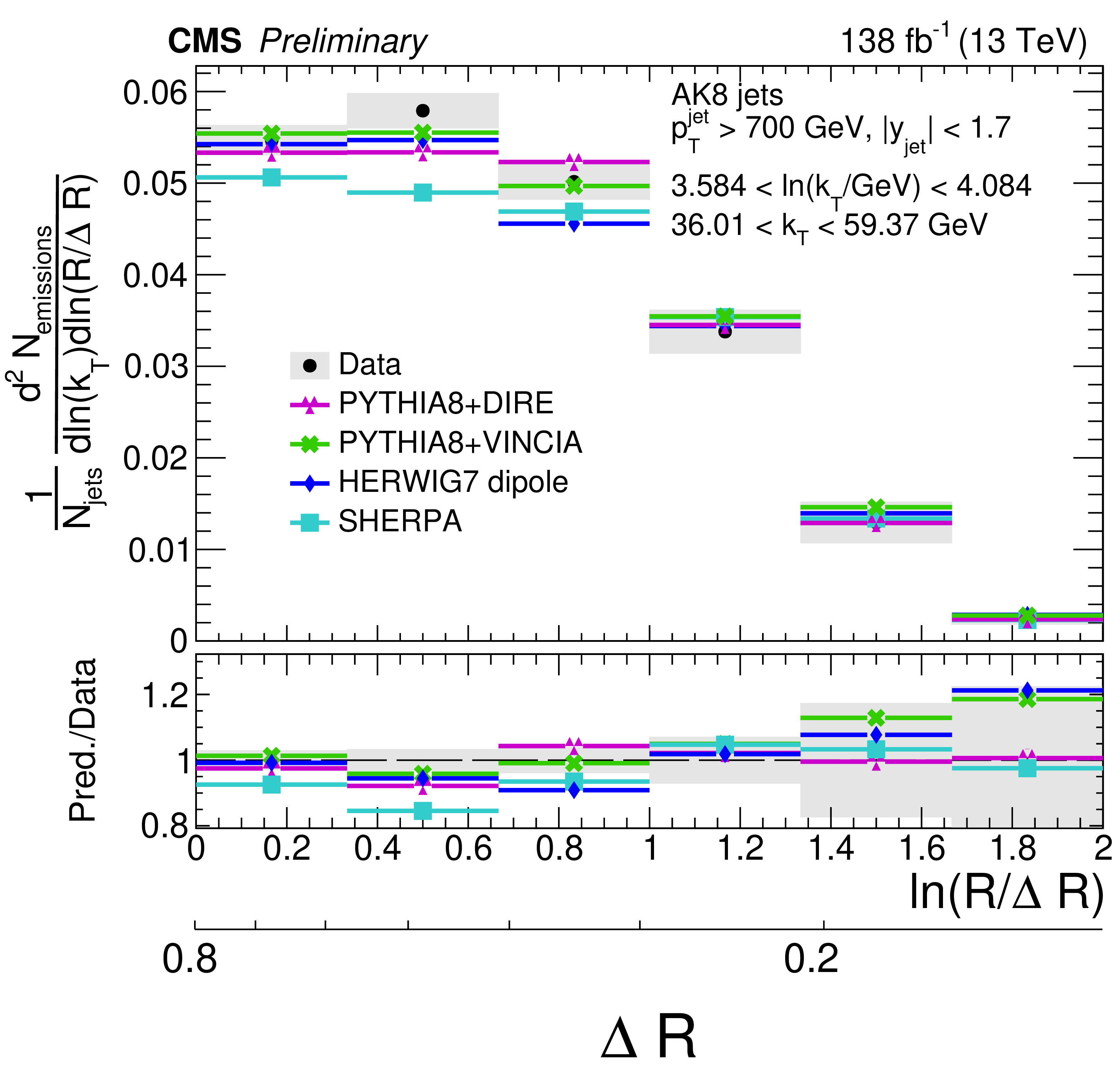
Four different slices of the primary Lund jet plane density of AK8 jets compared to predictions by PYTHIA8 + VINCIA, PYTHIA8+ DIRE, HERWIG 7 with dipole shower, and SHERPA. The band represents the total experimental uncertainty. The upper two panels correspond to vertical slices of the Lund jet plane for fixed $ \ln(R/\Delta R) $ (large angles on upper left, small angles on upper right). The lower two panels correspond to two different horizontal slices for fixed $ \ln(k_{\mathrm{T}}/\,\text{GeV}) $: the lower left panel corresponds to low $ k_{\mathrm{T}} $ splittings and spans the full range in $ \ln(R/\Delta R) $, whereas the lower right panel corresponds to high-$ k_{\mathrm{T}} $ splittings, which populate mostly wide-angle radiation. |
png pdf |
Figure 11-a:
Four different slices of the primary Lund jet plane density of AK8 jets compared to predictions by PYTHIA8 + VINCIA, PYTHIA8+ DIRE, HERWIG 7 with dipole shower, and SHERPA. The band represents the total experimental uncertainty. The upper two panels correspond to vertical slices of the Lund jet plane for fixed $ \ln(R/\Delta R) $ (large angles on upper left, small angles on upper right). The lower two panels correspond to two different horizontal slices for fixed $ \ln(k_{\mathrm{T}}/\,\text{GeV}) $: the lower left panel corresponds to low $ k_{\mathrm{T}} $ splittings and spans the full range in $ \ln(R/\Delta R) $, whereas the lower right panel corresponds to high-$ k_{\mathrm{T}} $ splittings, which populate mostly wide-angle radiation. |
png pdf |
Figure 11-b:
Four different slices of the primary Lund jet plane density of AK8 jets compared to predictions by PYTHIA8 + VINCIA, PYTHIA8+ DIRE, HERWIG 7 with dipole shower, and SHERPA. The band represents the total experimental uncertainty. The upper two panels correspond to vertical slices of the Lund jet plane for fixed $ \ln(R/\Delta R) $ (large angles on upper left, small angles on upper right). The lower two panels correspond to two different horizontal slices for fixed $ \ln(k_{\mathrm{T}}/\,\text{GeV}) $: the lower left panel corresponds to low $ k_{\mathrm{T}} $ splittings and spans the full range in $ \ln(R/\Delta R) $, whereas the lower right panel corresponds to high-$ k_{\mathrm{T}} $ splittings, which populate mostly wide-angle radiation. |
png pdf |
Figure 11-c:
Four different slices of the primary Lund jet plane density of AK8 jets compared to predictions by PYTHIA8 + VINCIA, PYTHIA8+ DIRE, HERWIG 7 with dipole shower, and SHERPA. The band represents the total experimental uncertainty. The upper two panels correspond to vertical slices of the Lund jet plane for fixed $ \ln(R/\Delta R) $ (large angles on upper left, small angles on upper right). The lower two panels correspond to two different horizontal slices for fixed $ \ln(k_{\mathrm{T}}/\,\text{GeV}) $: the lower left panel corresponds to low $ k_{\mathrm{T}} $ splittings and spans the full range in $ \ln(R/\Delta R) $, whereas the lower right panel corresponds to high-$ k_{\mathrm{T}} $ splittings, which populate mostly wide-angle radiation. |
png pdf |
Figure 11-d:
Four different slices of the primary Lund jet plane density of AK8 jets compared to predictions by PYTHIA8 + VINCIA, PYTHIA8+ DIRE, HERWIG 7 with dipole shower, and SHERPA. The band represents the total experimental uncertainty. The upper two panels correspond to vertical slices of the Lund jet plane for fixed $ \ln(R/\Delta R) $ (large angles on upper left, small angles on upper right). The lower two panels correspond to two different horizontal slices for fixed $ \ln(k_{\mathrm{T}}/\,\text{GeV}) $: the lower left panel corresponds to low $ k_{\mathrm{T}} $ splittings and spans the full range in $ \ln(R/\Delta R) $, whereas the lower right panel corresponds to high-$ k_{\mathrm{T}} $ splittings, which populate mostly wide-angle radiation. |
png pdf |
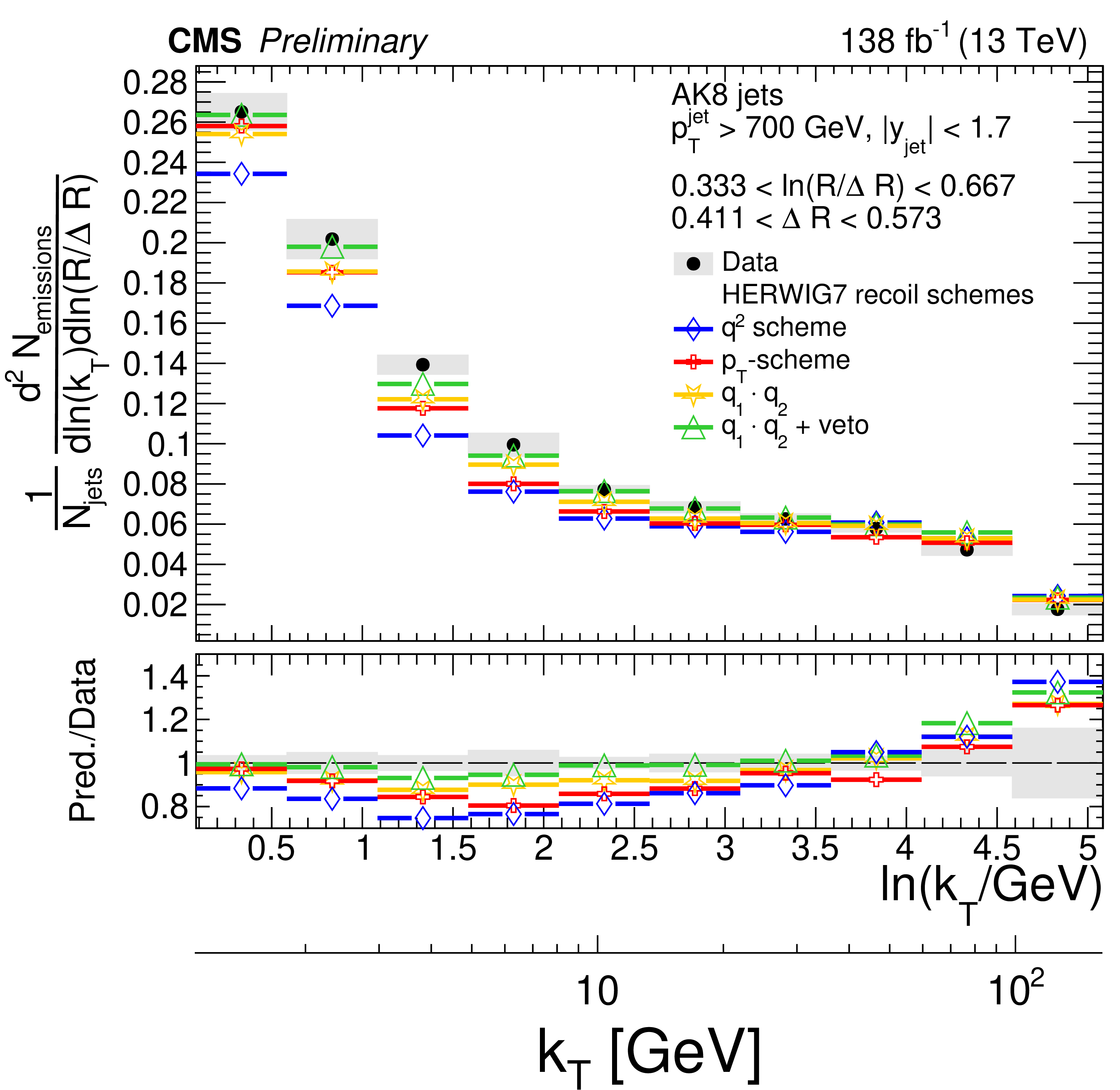
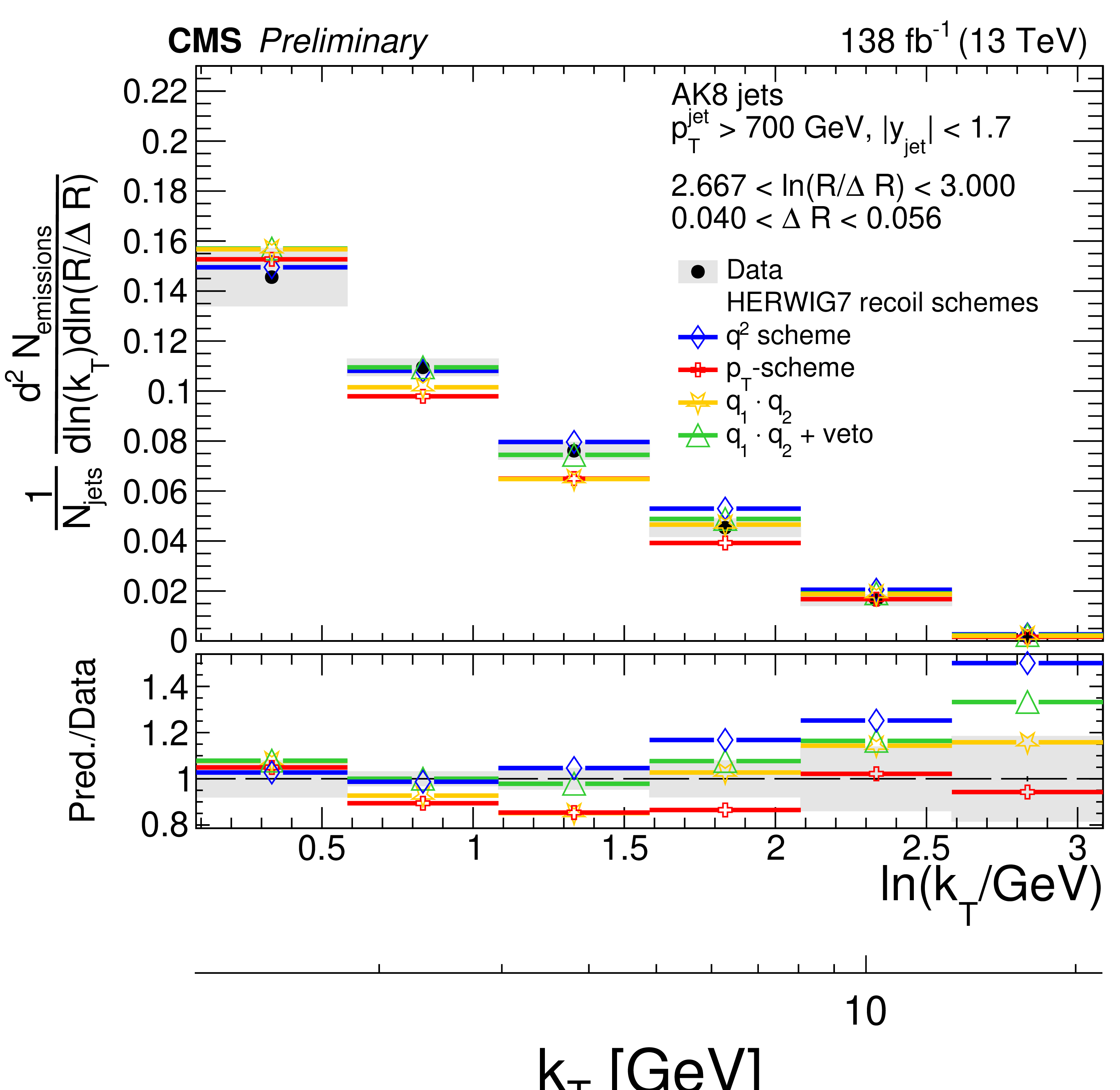
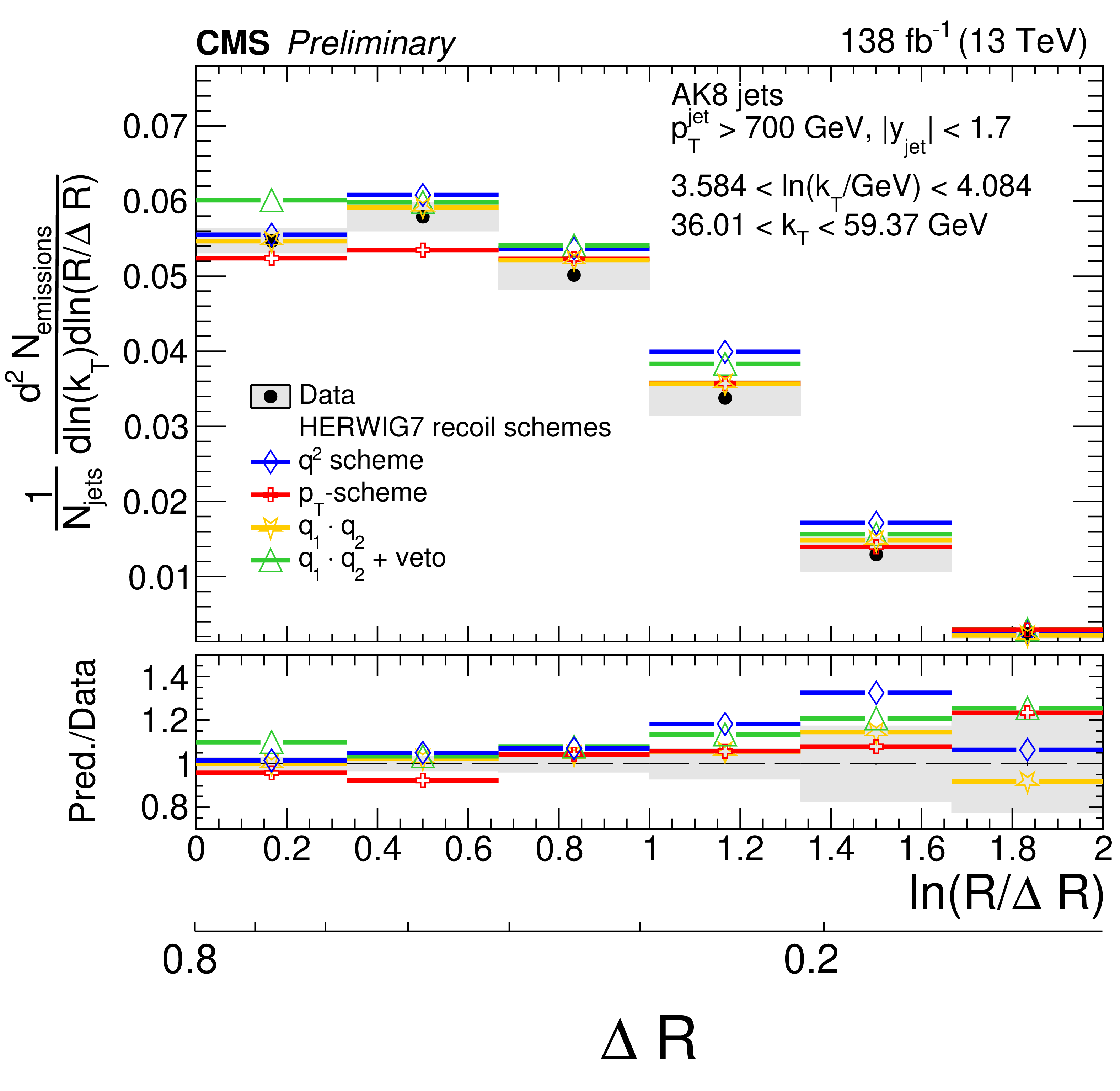
Figure 12:
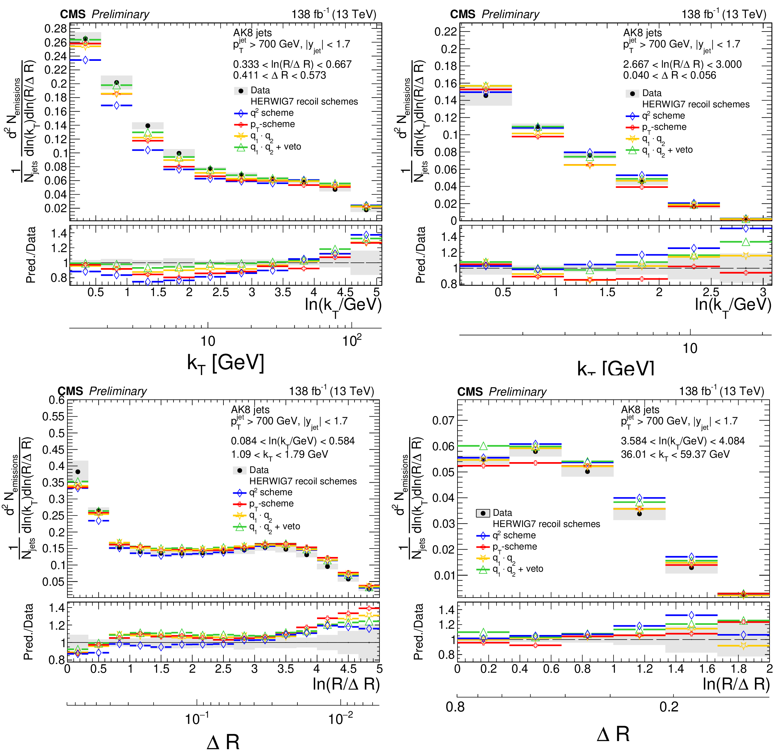
Four different slices of the primary Lund jet plane density of AK8 jets compared to predictions based on different choices of the recoil scheme of the angular ordered shower of HERWIG 7. The band represents the total experimental uncertainty. The upper two panels correspond to vertical slices of the Lund jet plane for fixed $ \ln(R/\Delta R) $ (large angles on upper left, small angles on upper right). The lower two panels correspond to two different horizontal slices for fixed $ k_{\mathrm{T}} $ interval: the lower left panel corresponds to low $ k_{\mathrm{T}} $ splittings and spans the full range in $ \ln(R/\Delta R) $, whereas the lower right panel corresponds to high-$ k_{\mathrm{T}} $ splittings, which populate mostly wide-angle radiation. |
png pdf |
Figure 12-a:
Four different slices of the primary Lund jet plane density of AK8 jets compared to predictions based on different choices of the recoil scheme of the angular ordered shower of HERWIG 7. The band represents the total experimental uncertainty. The upper two panels correspond to vertical slices of the Lund jet plane for fixed $ \ln(R/\Delta R) $ (large angles on upper left, small angles on upper right). The lower two panels correspond to two different horizontal slices for fixed $ k_{\mathrm{T}} $ interval: the lower left panel corresponds to low $ k_{\mathrm{T}} $ splittings and spans the full range in $ \ln(R/\Delta R) $, whereas the lower right panel corresponds to high-$ k_{\mathrm{T}} $ splittings, which populate mostly wide-angle radiation. |
png pdf |
Figure 12-b:
Four different slices of the primary Lund jet plane density of AK8 jets compared to predictions based on different choices of the recoil scheme of the angular ordered shower of HERWIG 7. The band represents the total experimental uncertainty. The upper two panels correspond to vertical slices of the Lund jet plane for fixed $ \ln(R/\Delta R) $ (large angles on upper left, small angles on upper right). The lower two panels correspond to two different horizontal slices for fixed $ k_{\mathrm{T}} $ interval: the lower left panel corresponds to low $ k_{\mathrm{T}} $ splittings and spans the full range in $ \ln(R/\Delta R) $, whereas the lower right panel corresponds to high-$ k_{\mathrm{T}} $ splittings, which populate mostly wide-angle radiation. |

png pdf |
Figure 12-c:
Four different slices of the primary Lund jet plane density of AK8 jets compared to predictions based on different choices of the recoil scheme of the angular ordered shower of HERWIG 7. The band represents the total experimental uncertainty. The upper two panels correspond to vertical slices of the Lund jet plane for fixed $ \ln(R/\Delta R) $ (large angles on upper left, small angles on upper right). The lower two panels correspond to two different horizontal slices for fixed $ k_{\mathrm{T}} $ interval: the lower left panel corresponds to low $ k_{\mathrm{T}} $ splittings and spans the full range in $ \ln(R/\Delta R) $, whereas the lower right panel corresponds to high-$ k_{\mathrm{T}} $ splittings, which populate mostly wide-angle radiation. |
png pdf |
Figure 12-d:
Four different slices of the primary Lund jet plane density of AK8 jets compared to predictions based on different choices of the recoil scheme of the angular ordered shower of HERWIG 7. The band represents the total experimental uncertainty. The upper two panels correspond to vertical slices of the Lund jet plane for fixed $ \ln(R/\Delta R) $ (large angles on upper left, small angles on upper right). The lower two panels correspond to two different horizontal slices for fixed $ k_{\mathrm{T}} $ interval: the lower left panel corresponds to low $ k_{\mathrm{T}} $ splittings and spans the full range in $ \ln(R/\Delta R) $, whereas the lower right panel corresponds to high-$ k_{\mathrm{T}} $ splittings, which populate mostly wide-angle radiation. |
png pdf |
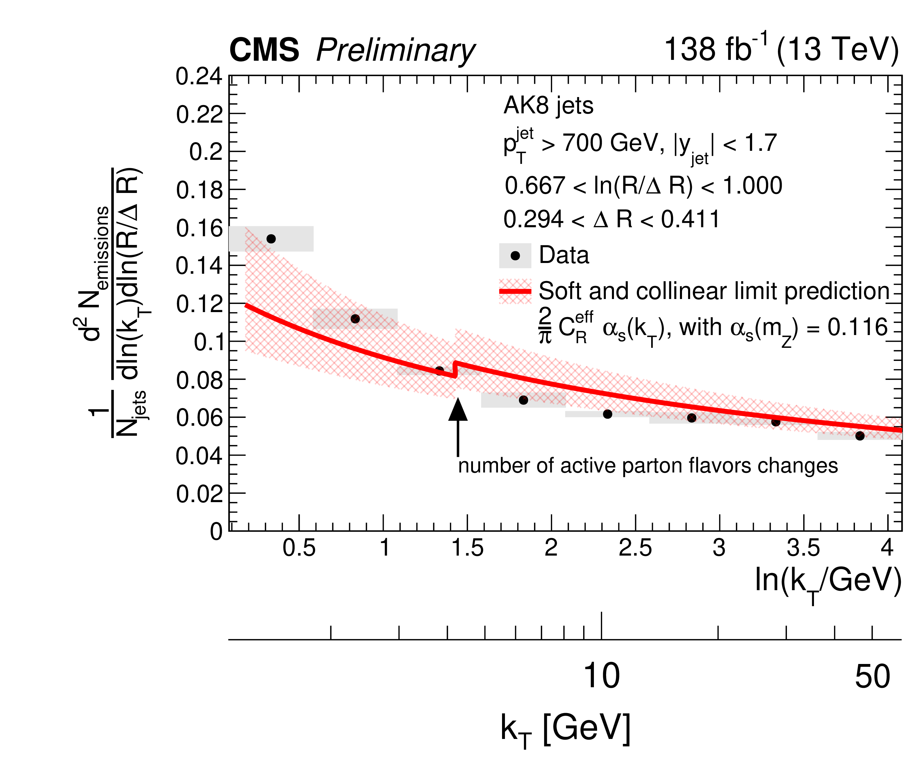
Figure 13:
Measured Lund jet plane distribution for AK8 jets, compared to the leading-order pQCD asymptotic prediction in the soft and collinear limit. An effective color factor of $ C_\mathrm{R}^\mathrm{eff} = $ 0.59 $C_\mathrm{F} + $ 0.41 $C_\mathrm{A} $ is assumed, as described in the text. The strong coupling $ \alpha_\mathrm{S} $ evolves with $ k_{\mathrm{T}} $ using the one-loop $ \beta $ function with $ \alpha_\mathrm{S} (m_\mathrm{Z}) = $ 0.116. The theoretical uncertainty band is calculated with variations of the renormalization scale by factors of 2. The discontinuity is due to the change of the number of active flavors when $ k_\mathrm{T} $ reaches the mass of the bottom quark, which is assumed to be 4.2 GeV. |
| Summary |
| In this note, we have presented a measurement of the primary Lund jet plane density in inclusive jet production in proton-proton (pp) collisions at 13 TeV using 138 fb$ ^{-1} $ of data collected with the CMS experiment. The primary Lund jet plane, a two-dimensional representation of the phase space of emissions inside the jet, is extracted using iterative Cambridge/Aachen jet declustering. The jet substructure is extracted using the charged-particle constituents of anti-$ k_{\mathrm{T}} $ jets with transverse momentum $ p_{\mathrm{T}} > $ 700 GeV and jet rapidity $ |y| < $ 1.7 with distance parameters of $ R = $ 0.4 or 0.8. The average density of emissions is measured as a function of the logarithm of the relative transverse momentum $ k_{\mathrm{T}} $ and the distance $ \Delta R $, and is fully corrected to stable particle level. The corrected distributions have an experimental uncertainty of 2--20%. The dependence on the parton shower and hadronization model is the dominant systematic uncertainty in the bulk of the Lund jet plane. Tracking inefficiencies become more important close to the kinematical edge of the Lund jet plane. The PYTHIA8 CP5 predictions systematically overestimate the Lund jet plane density at small $ k_{\mathrm{T}} $, which is the region dominated by hadronization. By choosing a smaller value of the renormalization scale in the evolution of the final-state radiation (FSR) shower, a better agreement of the PYTHIA8 CP5 tune is found in the perturbative region. The latter corresponds to effectively choosing a larger value of the strong coupling at the mass of the Z boson for FSR, $ \alpha_\mathrm{S}^\text{FSR}(m_\mathrm{Z}) $, which has been observed in other jet substructure measurements [72]. The HERWIG 7 predictions with the dot-product preserving recoil scheme, together with a veto on the virtuality of the partons at the end of the cascade, has the best global agreement with the data among the generators tested in the measurement. Predictions based on SHERPA, which has a dipole shower and cluster fragmentation model, is in agreement with the data in the bulk of the Lund jet plane, within 5--10%. The predictions from PYTHIA8 using the VINCIA and DIRE showers are generally in agreement with the data in the bulk of the Lund jet plane within 1--10% percent; they overestimate the density of emissions at low $ k_{\mathrm{T}} $ by 15--20%, as is the case for the standard shower of PYTHIA8. Finally, the PYTHIA8 predictions based on the Monash and CUEP8M1 tunes have in general a better agreement with the data than the predictions based on the CP tunes. For the most part, these differences are due to the different values of $ \alpha_\mathrm{S} $ used for FSR in the PYTHIA8 tunes tested in this measurement. These observations are qualitatively consistent with those made in a previous measurement of generalized angularities in Z+jets and dijet events at 13 TeV [75]. Since the measurement is corrected to particle level, it can be used as an input to improve the description from event generators and for future developments of parton showers with corrections beyond leading-logarithmic accuracy. |
| References | ||||
| 1 | A. J. Larkoski, I. Moult, and B. Nachman | Jet substructure at the Large Hadron Collider: a review of recent advances in theory and machine learning | Phys. Rept. 841 (2020) 1 | 1709.04464 |
| 2 | R. Kogler, B. Nachman, A. Schmidt (editors) et al. | Jet substructure at the Large Hadron Collider: experimental review | Rev. Mod. Phys. 91 (2019) 045003 | 1803.06991 |
| 3 | S. Marzani, G. Soyez, and M. Spannowsky | Looking inside jets: an introduction to jet substructure and boosted-object phenomenology | Lect. Notes Phys. 958 (2019) 1 | 1901.10342 |
| 4 | R. Kogler | Advances in jet substructure at the LHC: algorithms, measurements, and searches for new physical phenomena | volume 284. Springer, ISBN~978-3-030-72857-1, 978-3-030-72858-8 (2021) link |
|
| 5 | B. Andersson, G. Gustafson, L. Lonnblad, and U. Pettersson | Coherence Effects in Deep Inelastic Scattering | Z. Phys. C 43 (1989) 625 | |
| 6 | Y. L. Dokshitzer, G. D. Leder, S. Moretti, and B. R. Webber | Better jet clustering algorithms | JHEP 08 (1997) 001 | hep-ph/9707323 |
| 7 | M. Wobisch and T. Wengler | Hadronization corrections to jet cross-sections in deep inelastic scattering | in Workshop on Monte Carlo generators for HERA physics, 1998 link |
hep-ph/9907280 |
| 8 | F. A. Dreyer, G. P. Salam, and G. Soyez | The Lund jet plane | JHEP 12 (2018) 064 | 1807.04758 |
| 9 | H. A. Andrews et al. | Novel tools and observables for jet physics in heavy-ion collisions | JPG 47 (2020) 065102 | 1808.03689 |
| 10 | M. Cacciari, G. P. Salam, and G. Soyez | The anti-$ k_{\mathrm{T}} $ jet clustering algorithm | JHEP 04 (2008) 063 | 0802.1189 |
| 11 | M. Cacciari, G. P. Salam, and G. Soyez | FastJet user manual | EPJC 72 (2012) 1896 | 1111.6097 |
| 12 | A. Lifson, G. P. Salam, and G. Soyez | Calculating the primary Lund jet plane density | JHEP 10 (2020) 170 | 2007.06578 |
| 13 | M. Dasgupta et al. | Logarithmic accuracy of parton showers: a fixed-order study | JHEP 09 (2018) 033 | 1805.09327 |
| 14 | M. Dasgupta et al. | Parton showers beyond leading logarithmic accuracy | PRL 125 (2020) 052002 | 2002.11114 |
| 15 | K. Hamilton et al. | Color and logarithmic accuracy in final-state parton showers | JHEP 03 (2021) 041 | 2011.10054 |
| 16 | J. R. Forshaw, J. Holguin, and S. Plätzer | Building a consistent parton shower | JHEP 09 (2020) 014 | 2003.06400 |
| 17 | Z. Nagy and D. E. Soper | Summations by parton showers of large logarithms in electron-positron annihilation | 2011.04777 | |
| 18 | F. Herren et al. | A new approach to color-coherent parton evolution | 2208.06057 | |
| 19 | M. van Beekveld et al. | PanScales parton showers for hadron collisions: formulation and fixed-order studies | JHEP 11 (2022) 019 | 2205.02237 |
| 20 | M. van Beekveld et al. | PanScales showers for hadron collisions: all-order validation | JHEP 11 (2022) 020 | 2207.09467 |
| 21 | ALICE Collaboration | Direct observation of the dead-cone effect in quantum chromodynamics | Nature 605 (2022) 440 | 2106.05713 |
| 22 | F. A. Dreyer and H. Qu | Jet tagging in the Lund plane with graph networks | JHEP 03 (2021) 052 | 2012.08526 |
| 23 | L. Cavallini et al. | Tagging the Higgs boson decay to bottom quarks with color-sensitive observables and the Lund jet plane | EPJC 82 (2022) 493 | 2112.09650 |
| 24 | M. Dasgupta, A. Fregoso, S. Marzani, and G. P. Salam | Towards an understanding of jet substructure | JHEP 09 (2013) 029 | 1307.0007 |
| 25 | A. J. Larkoski, S. Marzani, G. Soyez, and J. Thaler | Soft Drop | JHEP 05 (2014) 146 | 1402.2657 |
| 26 | ATLAS Collaboration | Measurement of the Lund jet plane using charged particles in 13 TeV proton-proton collisions with the ATLAS detector | PRL 124 (2020) 222002 | 2004.03540 |
| 27 | ALICE Collaboration | Measurement of the primary Lund plane density in pp collisions at $ \sqrt{s} =$ 13 TeV with ALICE | ALICE Physics Preliminary Summary ALICE-PUBLIC-2021-002, 2021 | |
| 28 | CMS Collaboration | DeepCore: convolutional neural network for high $ p_{\mathrm{T}} $ jet tracking | CMS Detector Performance Note CMS-DP-2019-007, 2019 CDS |
|
| 29 | CMS Collaboration | Description and performance of track and primary-vertex reconstruction with the CMS tracker | JINST 9 (2014) P10009 | CMS-TRK-11-001 1405.6569 |
| 30 | CMS Tracker Group | The CMS phase-1 pixel detector upgrade | JINST 16 (2021) P02027 | 2012.14304 |
| 31 | CMS Collaboration | Track impact parameter resolution for the full pseudo rapidity coverage in the 2017 dataset with the CMS phase-1 pixel detector | CMS Detector Performance Summary CMS-DP-2020-049, 2020 CDS |
|
| 32 | CMS Collaboration | Performance of the CMS muon detector and muon reconstruction with proton-proton collisions at $ \sqrt{s} = $ 13 TeV | JINST 13 (2018) P06015 | CMS-MUO-16-001 1804.04528 |
| 33 | CMS Collaboration | Particle-flow reconstruction and global event description with the CMS detector | JINST 12 (2017) P10003 | CMS-PRF-14-001 1706.04965 |
| 34 | CMS Collaboration | Jet energy scale and resolution in the CMS experiment in pp collisions at 8 TeV | JINST 12 (2017) P02014 | CMS-JME-13-004 1607.03663 |
| 35 | CMS Collaboration | Pileup mitigation at CMS in 13 TeV data | JINST 15 (2020) P09018 | CMS-JME-18-001 2003.00503 |
| 36 | CMS Collaboration | The CMS trigger system | JINST 12 (2017) P01020 | CMS-TRG-12-001 1609.02366 |
| 37 | CMS Collaboration | Performance of the CMS level-1 trigger in proton-proton collisions at $ \sqrt{s} = $ 13 TeV | JINST 15 (2020) P10017 | CMS-TRG-17-001 2006.10165 |
| 38 | CMS Collaboration | The CMS experiment at the CERN LHC | JINST 3 (2008) S08004 | |
| 39 | T. Sjöstrand et al. | An introduction to PYTHIA 8.2 | Comput. Phys. Commun. 191 (2015) 159 | 1410.3012 |
| 40 | B. Andersson, G. Gustafson, G. Ingelman, and T. Sjöstrand | Parton fragmentation and string dynamics | Phys. Rept. 97 (1983) 31 | |
| 41 | T. Sjöstrand | The merging of jets | PLB 142 (1984) 420 | |
| 42 | CMS Collaboration | Extraction and validation of a new set of CMS PYTHIA 8 tunes from underlying-event measurements | EPJC 80 (2020) 4 | CMS-GEN-17-001 1903.12179 |
| 43 | NNPDF Collaboration | Parton distributions for the LHC Run II | JHEP 04 (2015) 040 | 1410.8849 |
| 44 | CMS Collaboration | Development and validation of HERWIG 7 tunes from CMS underlying-event measurements | EPJC 81 (2021) 312 | CMS-GEN-19-001 2011.03422 |
| 45 | S. Gieseke, P. Stephens, and B. Webber | New formalism for QCD parton showers | JHEP 12 (2003) 045 | hep-ph/0310083 |
| 46 | B. R. Webber | A QCD model for jet fragmentation including soft gluon interference | NPB 238 (1984) 492 | |
| 47 | GEANT4 Collaboration | GEANT 4---a simulation toolkit | NIM A 506 (2003) 250 | |
| 48 | P. Skands, S. Carrazza, and J. Rojo | Tuning PYTHIA8.1: The Monash 2013 tune | EPJC 74 (2014) 3024 | 1404.5630 |
| 49 | CMS Collaboration | Event generator tunes obtained from underlying event and multiparton scattering measurements | EPJC 76 (2016) 155 | CMS-GEN-14-001 1512.00815 |
| 50 | S. Höche and S. Prestel | The midpoint between dipole and parton showers | EPJC 75 (2015) 461 | 1506.05057 |
| 51 | W. T. Giele, D. A. Kosower, and P. Z. Skands | A simple shower and matching algorithm | PRD 78 (2008) 014026 | 0707.3652 |
| 52 | A. Gehrmann-De Ridder, T. Gehrmann, and E. W. N. Glover | Antenna subtraction at NNLO | JHEP 09 (2005) 056 | hep-ph/0505111 |
| 53 | H. Brooks, C. T. Preuss, and P. Skands | Sector showers for hadron collisions | JHEP 07 (2020) 032 | 2003.00702 |
| 54 | J. Bellm et al. | HERWIG 7.0/HERWIG++ 3.0 release note | EPJC 76 (2016) 196 | 1512.01178 |
| 55 | J. Bellm et al. | HERWIG 7.2 release note | EPJC 80 (2020) 452 | 1912.06509 |
| 56 | S. Catani and M. H. Seymour | A general algorithm for calculating jet cross-sections in NLO QCD | NPB 485 (1997) 291 | hep-ph/9605323 |
| 57 | Sherpa Collaboration | Event generation with Sherpa 2.2 | SciPost Phys. 7 (2019) 034 | 1905.09127 |
| 58 | F. Krauss, R. Kuhn, and G. Soff | AMEGIC++ 1.0: a matrix element generator in C++ | JHEP 02 (2002) 044 | hep-ph/0109036 |
| 59 | T. Gleisberg and S. Höche | Comix, a new matrix element generator | JHEP 12 (2008) 039 | 0808.3674 |
| 60 | S. Schumann and F. Krauss | A parton shower algorithm based on Catani-Seymour dipole factorisation | JHEP 03 (2008) 038 | 0709.1027 |
| 61 | J.-C. Winter, F. Krauss, and G. Soff | A modified cluster hadronization model | EPJC 36 (2004) 381 | hep-ph/0311085 |
| 62 | G. Bewick, S. Ferrario Ravasio, P. Richardson, and M. H. Seymour | Logarithmic accuracy of angular-ordered parton showers | JHEP 04 (2020) 019 | 1904.11866 |
| 63 | T. Sjöstrand and M. van Zijl | A multiple interaction model for the event structure in hadron collisions | PRD 36 (1987) 2019 | |
| 64 | J. M. Butterworth, J. R. Forshaw, and M. H. Seymour | Multiparton interactions in photoproduction at HERA | Z. Phys. C 72 (1996) 637 | hep-ph/9601371 |
| 65 | I. Borozan and M. H. Seymour | An eikonal model for multiparticle production in hadron hadron interactions | JHEP 09 (2002) 015 | hep-ph/0207283 |
| 66 | M. Bahr, S. Gieseke, and M. H. Seymour | Simulation of multiple partonic interactions in HERWIG ++ | JHEP 07 (2008) 076 | 0803.3633 |
| 67 | S. Gieseke, C. Rohr, and A. Siodmok | Colour reconnections in HERWIG ++ | EPJC 72 (2012) 2225 | 1206.0041 |
| 68 | G. D'Agostini | A multidimensional unfolding method based on Bayes' theorem | NIM A 362 (1995) 487 | |
| 69 | T. Adye | Unfolding algorithms and tests using RooUnfold | in Workshop on Statistical Issues Related to Discovery Claims in Search Experiments and Unfolding, H. Prosper and L. Lyons, eds., Geneva, 2011 PHYSTAT 2011 (2011) 313 |
1105.1160 |
| 70 | M. Cacciari et al. | The $ \mathrm{t} \bar{\mathrm{t}} $ cross-section at 1.8 TeV and 1.96 TeV: a study of the systematics due to parton densities and scale dependence | JHEP 04 (2004) 068 | hep-ph/0303085 |
| 71 | S. Catani, D. de Florian, M. Grazzini, and P. Nason | Soft gluon resummation for Higgs boson production at hadron colliders | JHEP 07 (2003) 028 | hep-ph/0306211 |
| 72 | CMS Collaboration | Measurement of the jet mass distribution and top quark mass in hadronic decays of boosted top quarks in proton-proton collisions at $ \sqrt{s} $ = 13 TeV | CMS-TOP-21-012 2211.01456 |
|
| 73 | CMS Collaboration | Jet algorithms performance in 13 TeV data | CMS Physics Analysis Summary, 2017 CMS-PAS-JME-16-003 |
CMS-PAS-JME-16-003 |
| 74 | Particle Data Group Collaboration | Review of particle physics | Prog. Theor. Exp. Phys. 2022 (2022) 083C01 | |
| 75 | CMS Collaboration | Study of quark and gluon jet substructure in Z+jet and dijet events from pp collisions | JHEP 01 (2022) 188 | CMS-SMP-20-010 2109.03340 |
|
|
Compact Muon Solenoid LHC, CERN |
|

|

|

|

|

|