

Compact Muon Solenoid
LHC, CERN
| CMS-PAS-SMP-18-012 | ||
| Measurement of the W boson rapidity, helicity, and differential cross sections in pp collisions at $\sqrt{s}= $ 13 TeV | ||
| CMS Collaboration | ||
| February 2020 | ||
| Abstract: The differential cross section and charge asymmetry for inclusive W boson production at $\sqrt{s}= $ 13 TeV is measured for the two transverse polarization states as a function of the W boson absolute rapidity. The measurement uses events in which a W boson decays to either an electron or a muon and a neutrino. The data sample of proton-proton collisions recorded with the CMS detector at the LHC in 2016 corresponds to an integrated luminosity of 35.9 fb$^{-1}$. The absolute differential cross section, and its value normalized to the total inclusive W boson production cross section, are measured over the rapidity range $| Y_{\mathrm{W}} | < $ 2.5. In addition, the W boson double-differential cross section, $\mathrm{d}^2\sigma/\mathrm{d}p_{\mathrm{T}}^{\ell} \mathrm{d}|\eta^{\ell}|$, and the charge asymmetry, are measured as a function of the charged lepton transverse momentum and pseudorapidity. The precision of these measurements is used to constrain the parton density functions (PDF) of the proton using the next-to-leading-order PDF set NNPDF3.0. | ||
|
Links:
CDS record (PDF) ;
CADI line (restricted) ;
These preliminary results are superseded in this paper, PRD 102 (2020) 092012. The superseded preliminary plots can be found here. |
||
| Figures & Tables | Summary | Additional Figures | References | CMS Publications |
|---|
| Figures | |

png pdf |
Figure 1:
Distributions of the W boson ${p_{\mathrm {T}} ^{\mathrm{W}}}$ (left), ${| Y_{\mathrm{W}} |}$ (center), and the resulting $\eta $ distribution of the charged lepton (right) after reweighting each of the helicity components for positive (top row) and negative charge (bottom row) W bosons. |
png pdf |
Figure 1-a:
Distributions of the W boson ${p_{\mathrm {T}} ^{\mathrm{W}}}$ (left), ${| Y_{\mathrm{W}} |}$ (center), and the resulting $\eta $ distribution of the charged lepton (right) after reweighting each of the helicity components for positive (top row) and negative charge (bottom row) W bosons. |

png pdf |
Figure 1-b:
Distributions of the W boson ${p_{\mathrm {T}} ^{\mathrm{W}}}$ (left), ${| Y_{\mathrm{W}} |}$ (center), and the resulting $\eta $ distribution of the charged lepton (right) after reweighting each of the helicity components for positive (top row) and negative charge (bottom row) W bosons. |
png pdf |
Figure 1-c:
Distributions of the W boson ${p_{\mathrm {T}} ^{\mathrm{W}}}$ (left), ${| Y_{\mathrm{W}} |}$ (center), and the resulting $\eta $ distribution of the charged lepton (right) after reweighting each of the helicity components for positive (top row) and negative charge (bottom row) W bosons. |
png pdf |
Figure 1-d:
Distributions of the W boson ${p_{\mathrm {T}} ^{\mathrm{W}}}$ (left), ${| Y_{\mathrm{W}} |}$ (center), and the resulting $\eta $ distribution of the charged lepton (right) after reweighting each of the helicity components for positive (top row) and negative charge (bottom row) W bosons. |

png pdf |
Figure 1-e:
Distributions of the W boson ${p_{\mathrm {T}} ^{\mathrm{W}}}$ (left), ${| Y_{\mathrm{W}} |}$ (center), and the resulting $\eta $ distribution of the charged lepton (right) after reweighting each of the helicity components for positive (top row) and negative charge (bottom row) W bosons. |
png pdf |
Figure 1-f:
Distributions of the W boson ${p_{\mathrm {T}} ^{\mathrm{W}}}$ (left), ${| Y_{\mathrm{W}} |}$ (center), and the resulting $\eta $ distribution of the charged lepton (right) after reweighting each of the helicity components for positive (top row) and negative charge (bottom row) W bosons. |
png pdf |
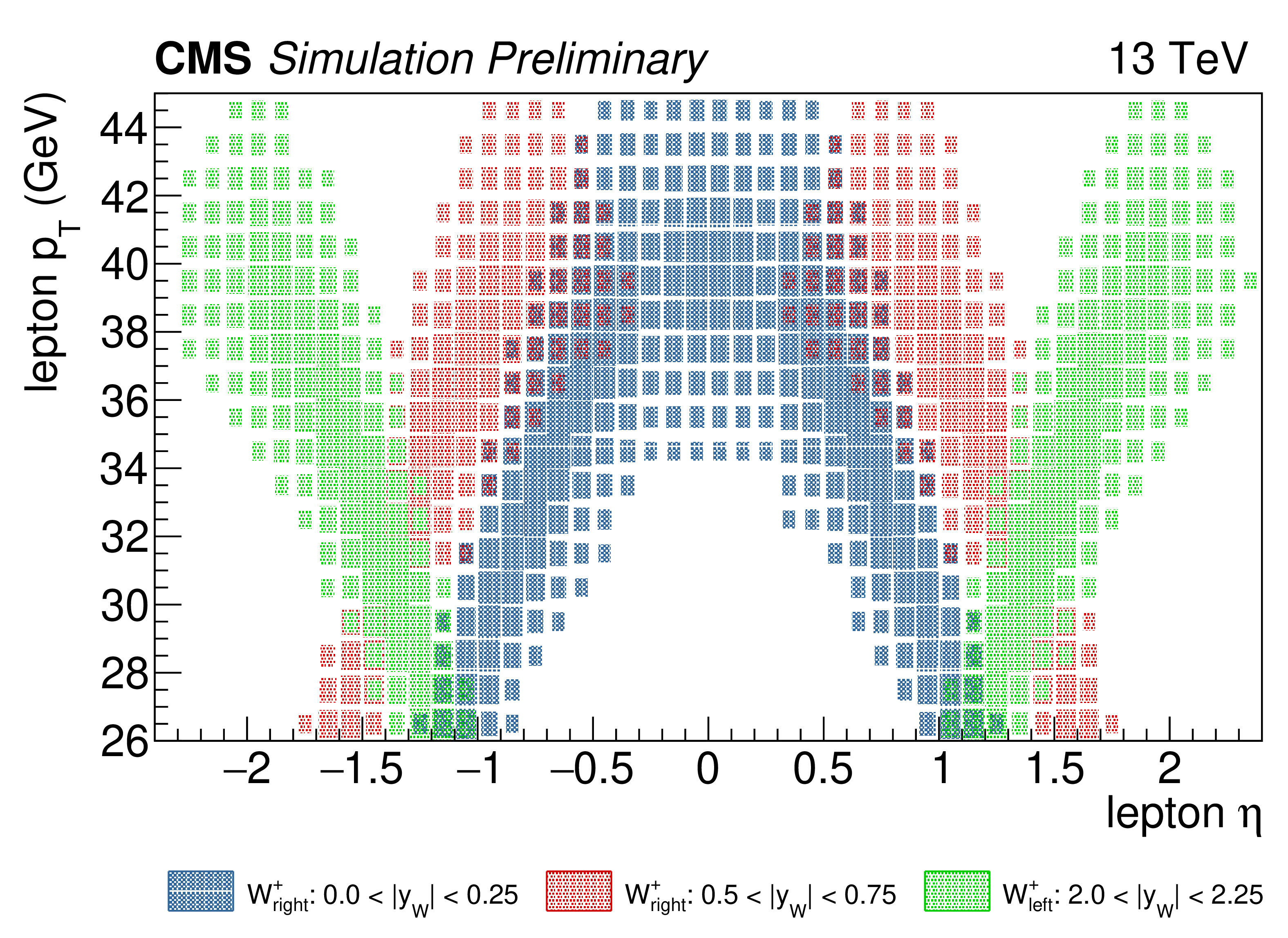
Figure 2:
Distributions of 2D templates of ${{p_{\mathrm {T}}} ^{\ell}}$ versus ${\eta ^{\ell}}$, for positively charged W boson simulated events with different helicity or rapidity bin. Blue: $ {\mathrm{W^{+}} _{R}} $ with $ {| Y_{\mathrm{W}} |} < $ 0.25, red: $ {\mathrm{W^{+}} _{R}} $ with 0.5 $ < {| Y_{\mathrm{W}} |} < $ 0.75, green: $ {\mathrm{W^{+}} _{L}} $ with 2.0 $ < {| Y_{\mathrm{W}} |} < $ 2.25. |
png pdf |
Figure 3:
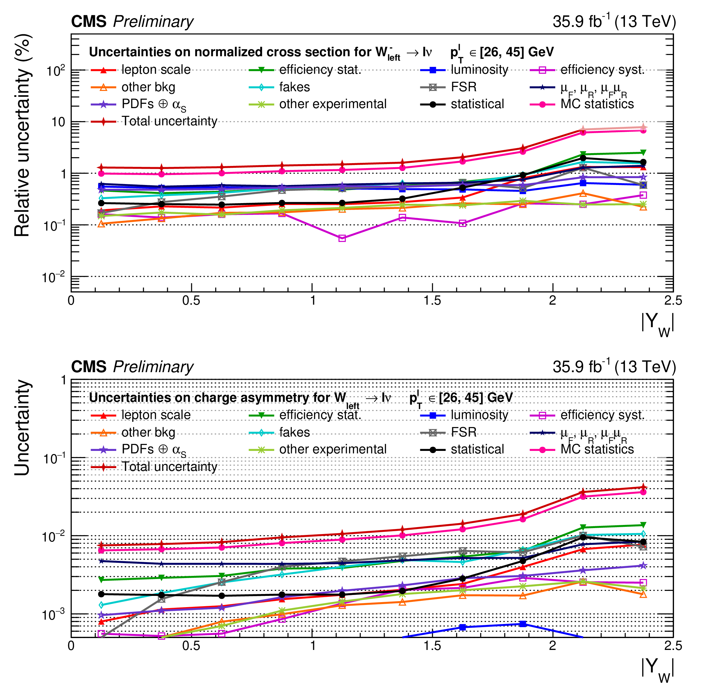
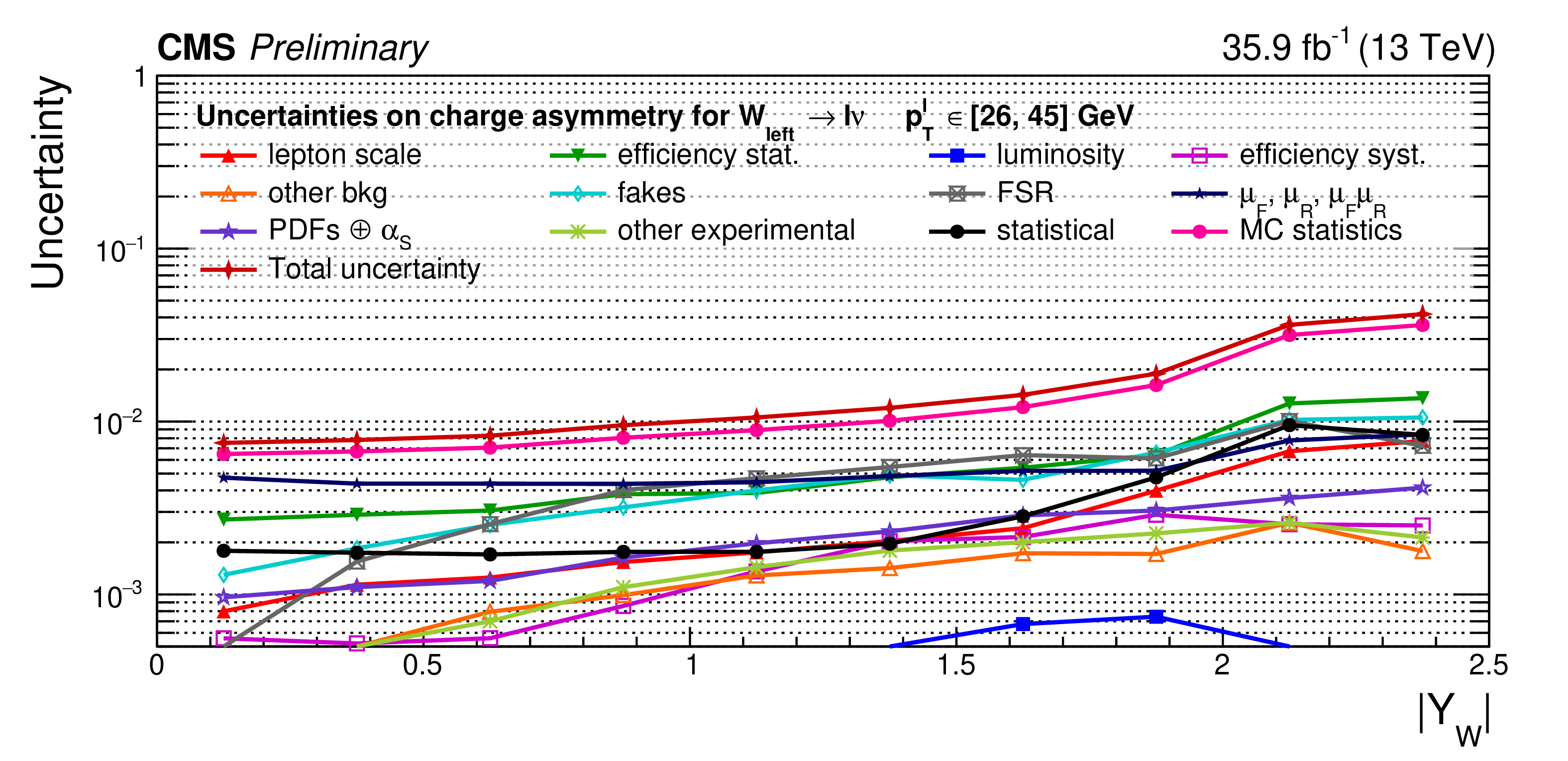
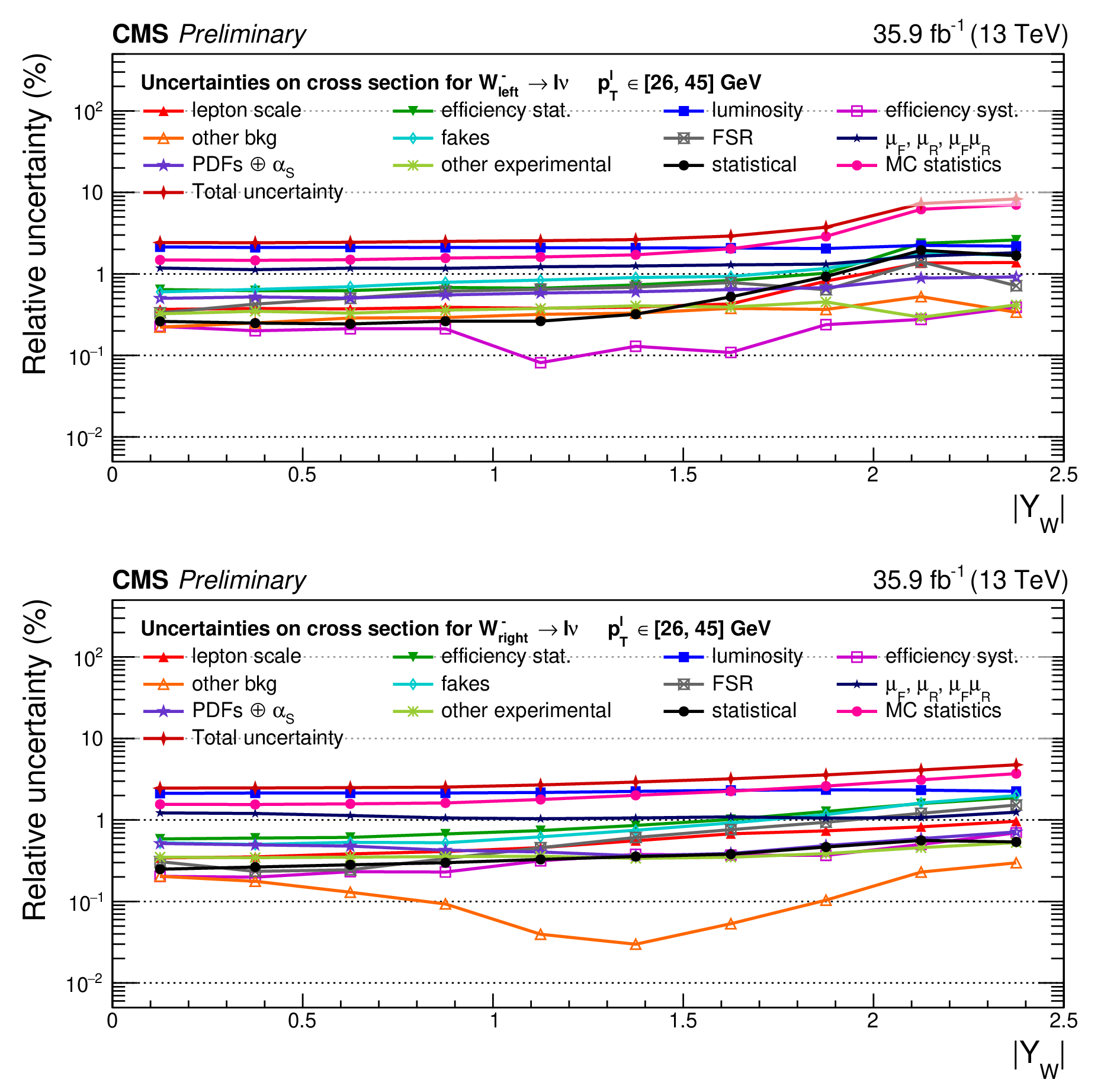
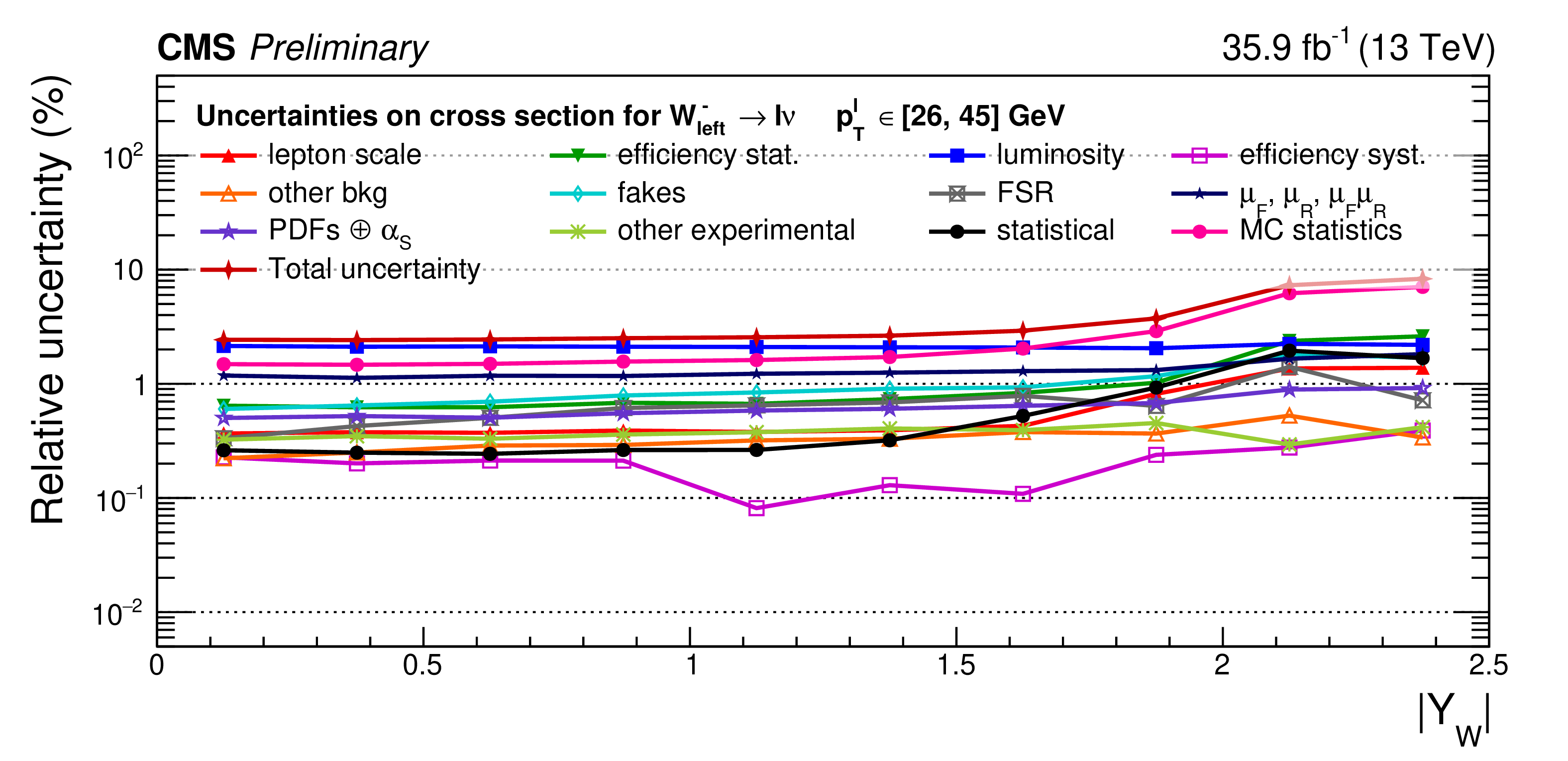
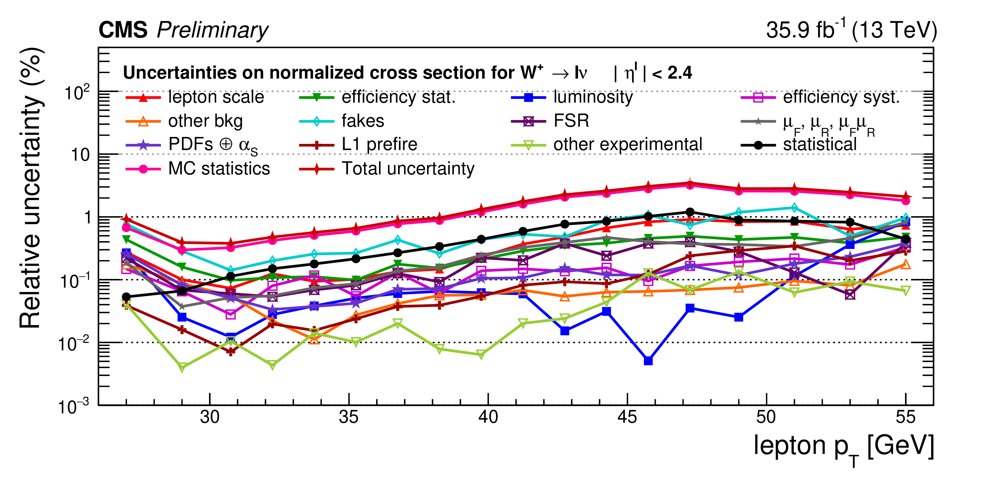
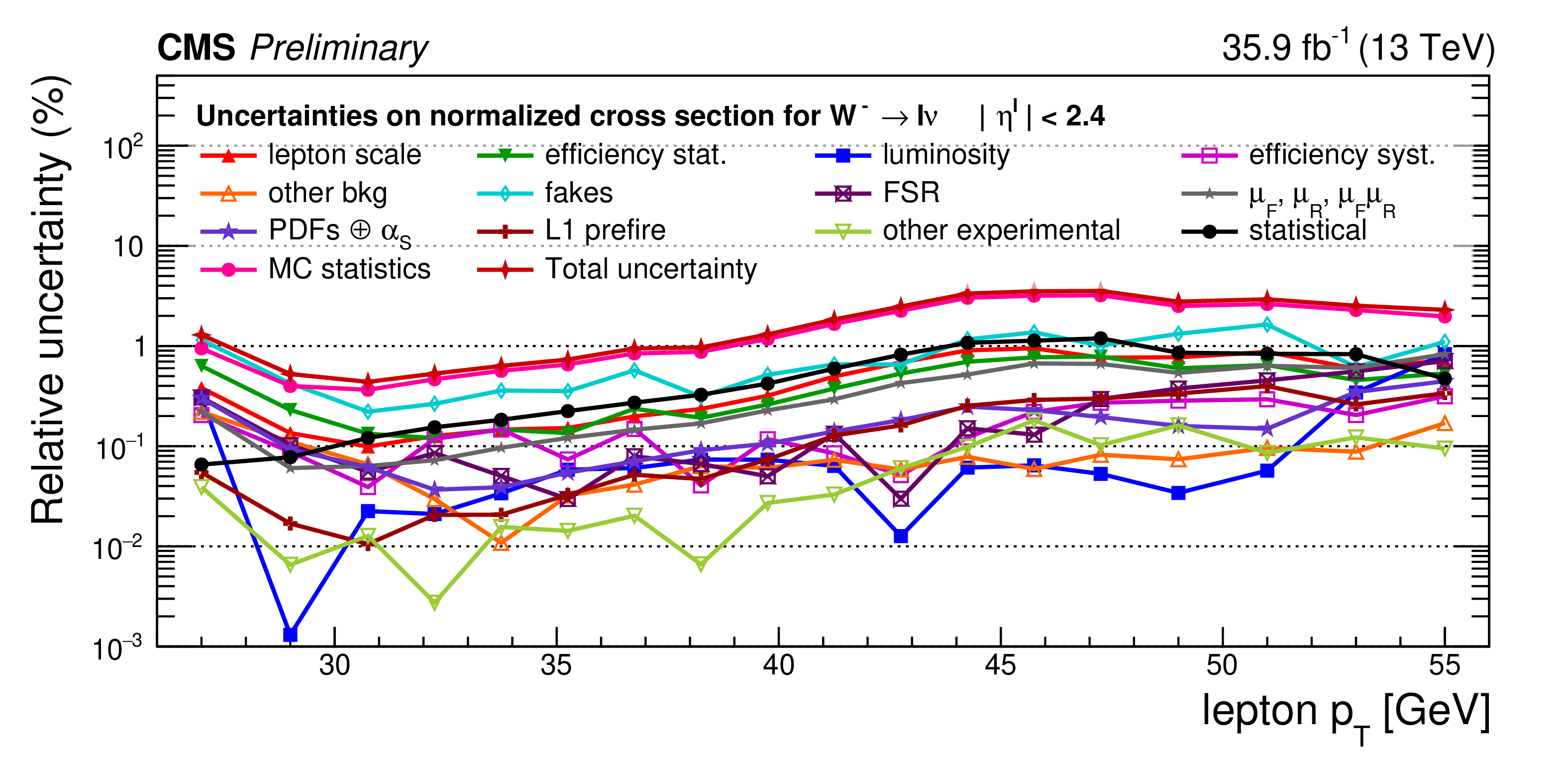
Top: relative impact of groups of uncertainties (as defined in the text) on the signal normalized cross sections for the $ {\mathrm{W^{-}} _{L}} $ case. Bottom: absolute impact of uncertainties on the charge asymmetry of $ {\mathrm{W} _{L}} $. All impacts are shown for the combination of the muon and electron channels. |

png pdf |
Figure 3-a:
Top: relative impact of groups of uncertainties (as defined in the text) on the signal normalized cross sections for the $ {\mathrm{W^{-}} _{L}} $ case. Bottom: absolute impact of uncertainties on the charge asymmetry of $ {\mathrm{W} _{L}} $. All impacts are shown for the combination of the muon and electron channels. |
png pdf |
Figure 3-b:
Top: relative impact of groups of uncertainties (as defined in the text) on the signal normalized cross sections for the $ {\mathrm{W^{-}} _{L}} $ case. Bottom: absolute impact of uncertainties on the charge asymmetry of $ {\mathrm{W} _{L}} $. All impacts are shown for the combination of the muon and electron channels. |
png pdf |
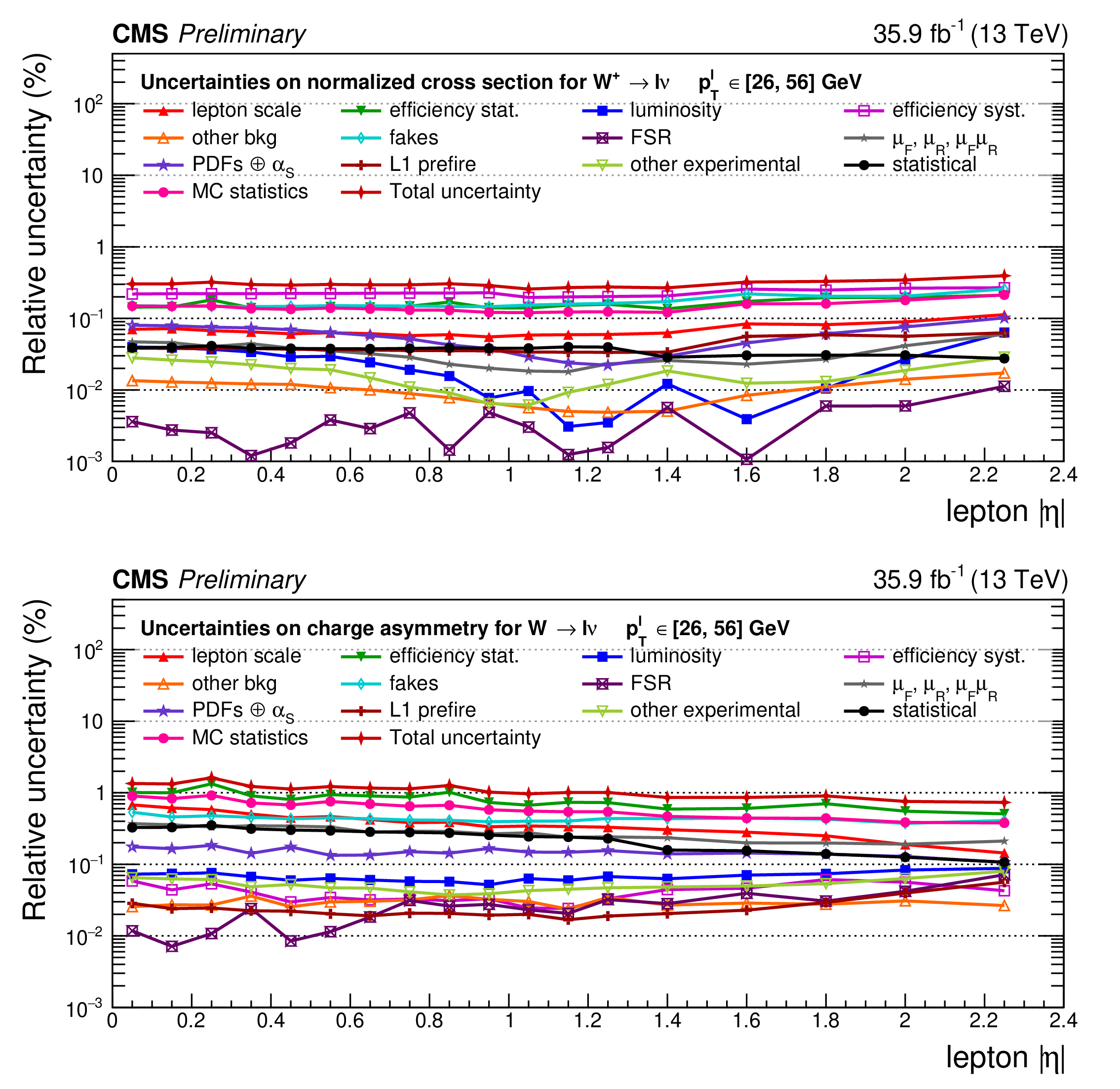
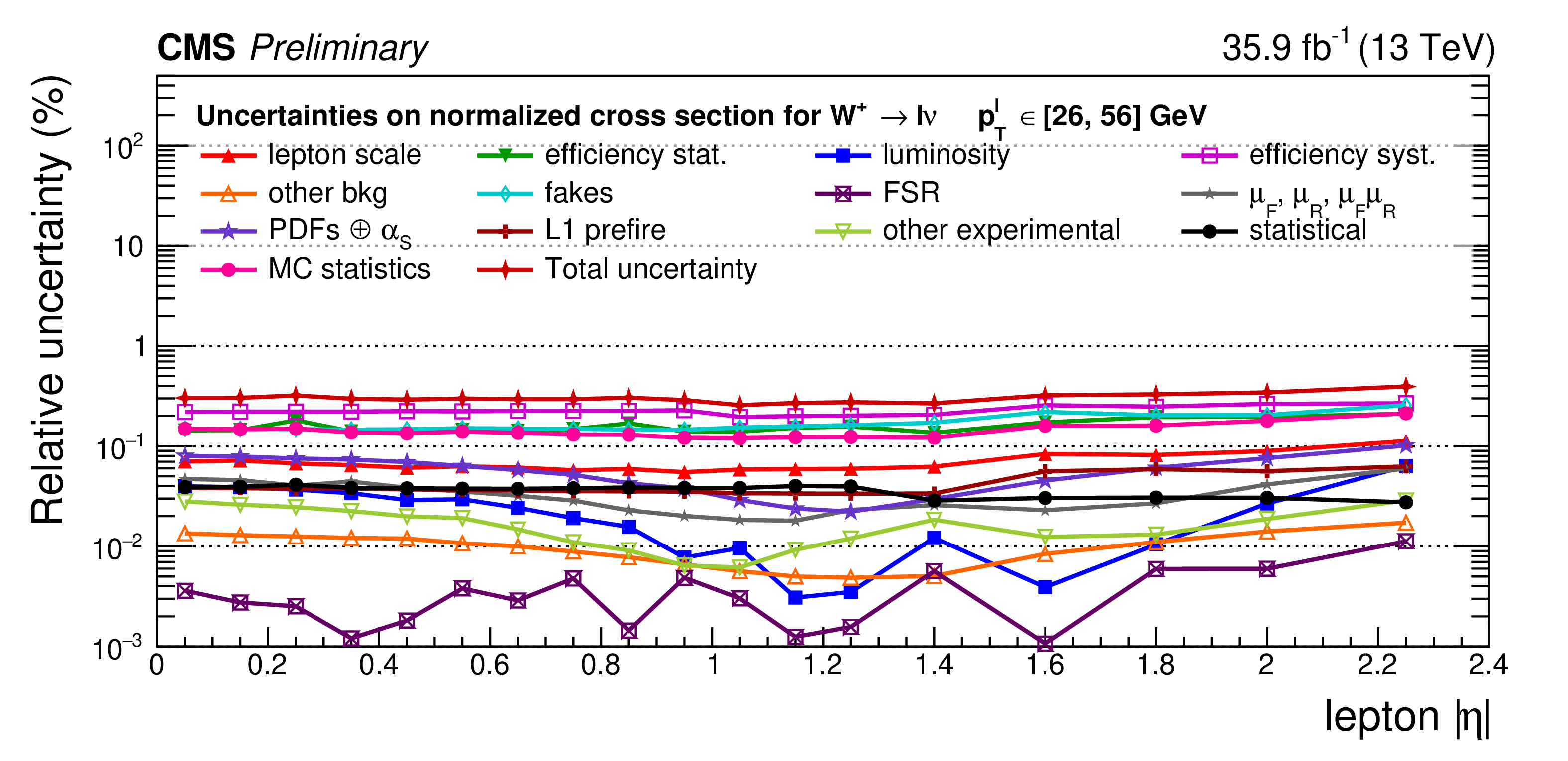
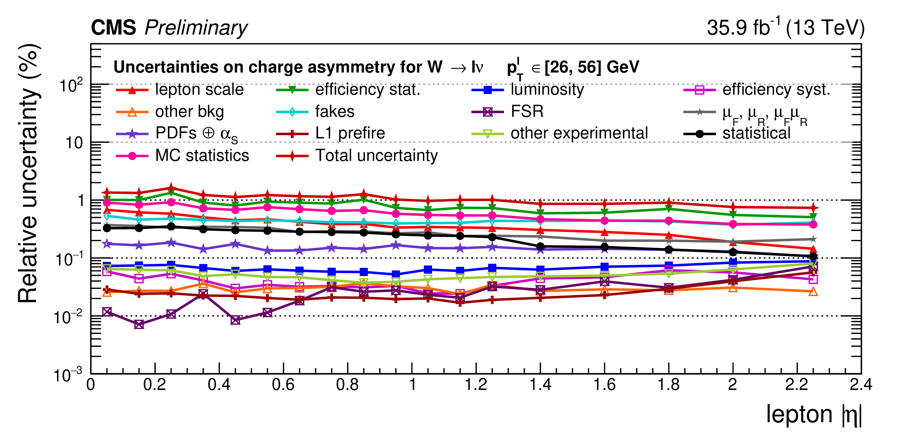
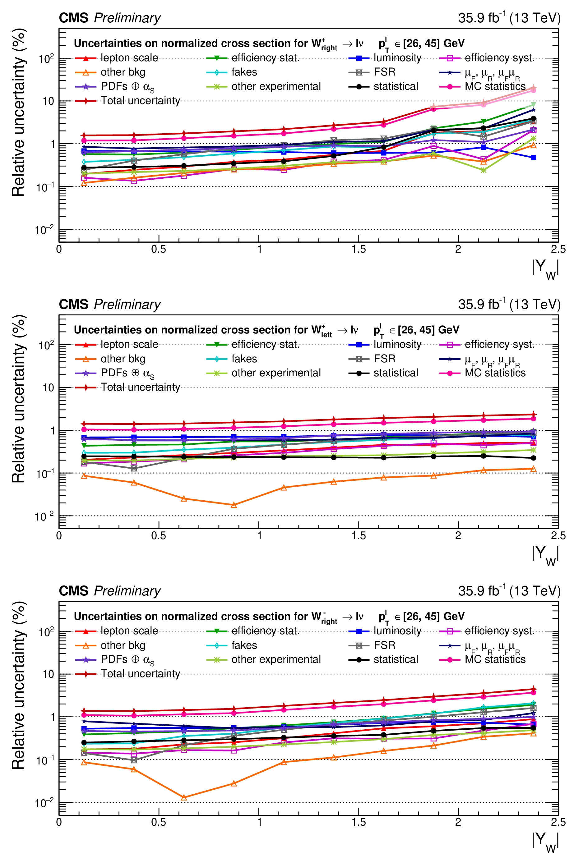
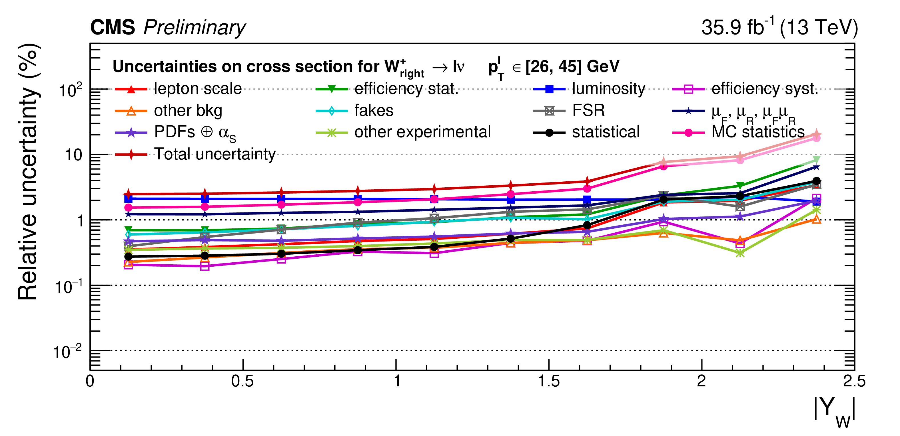
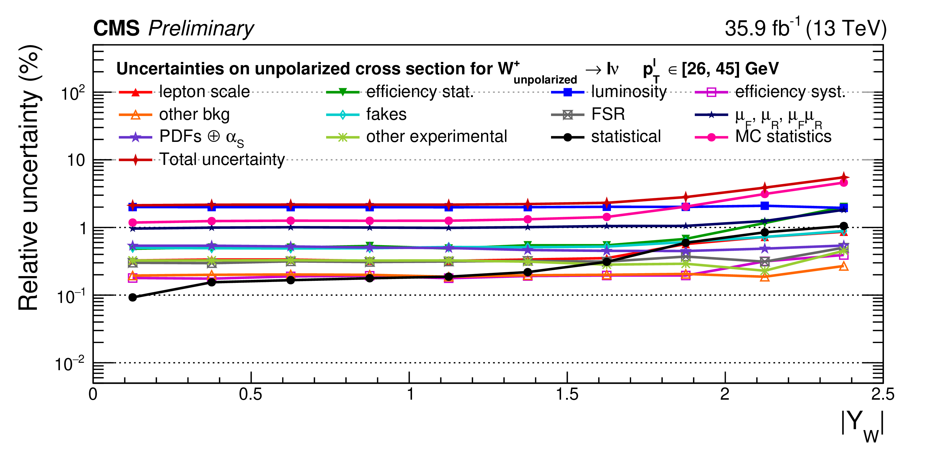
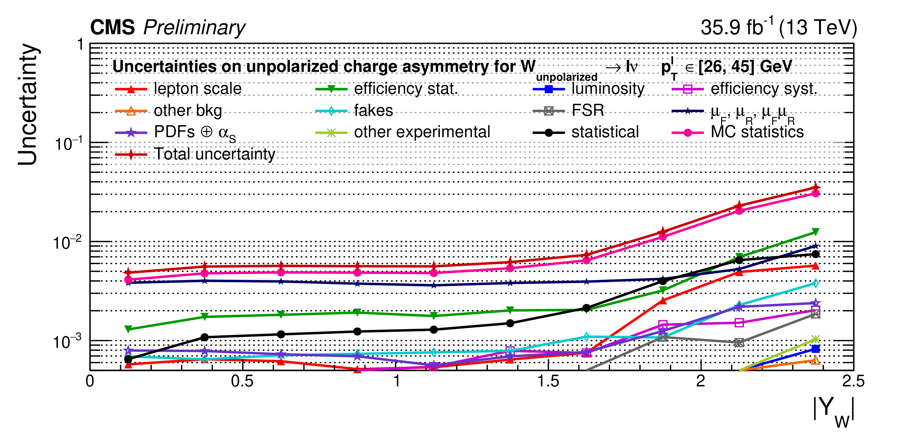
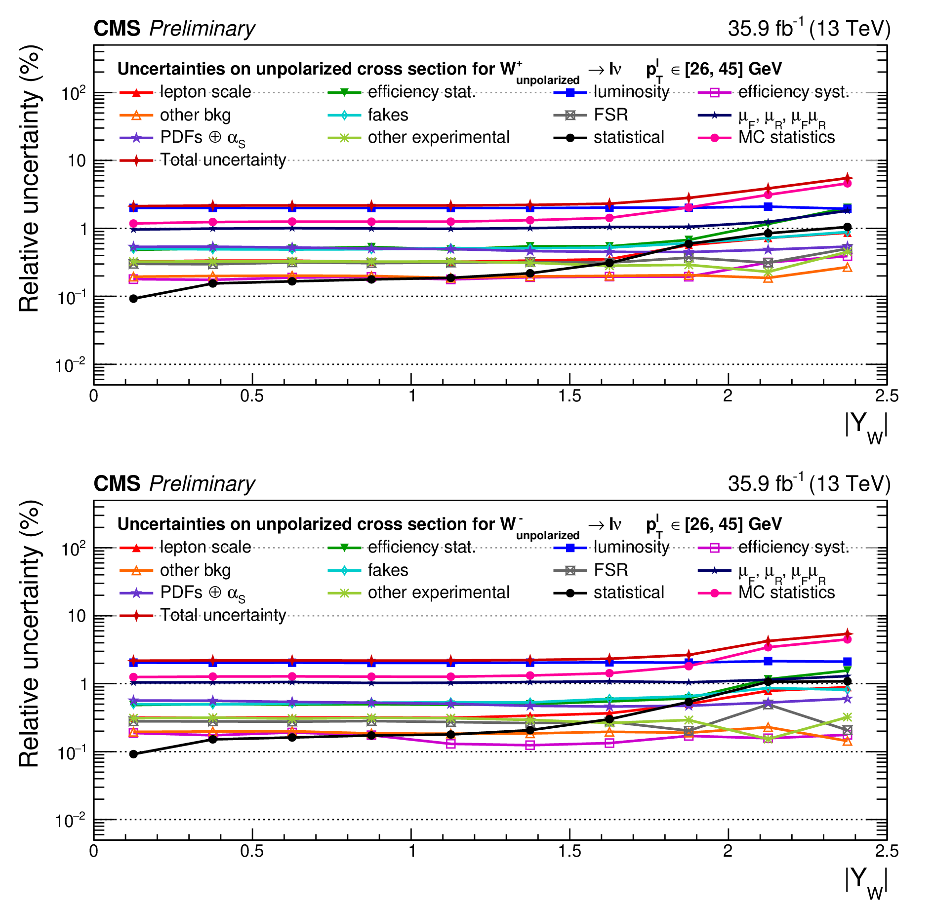
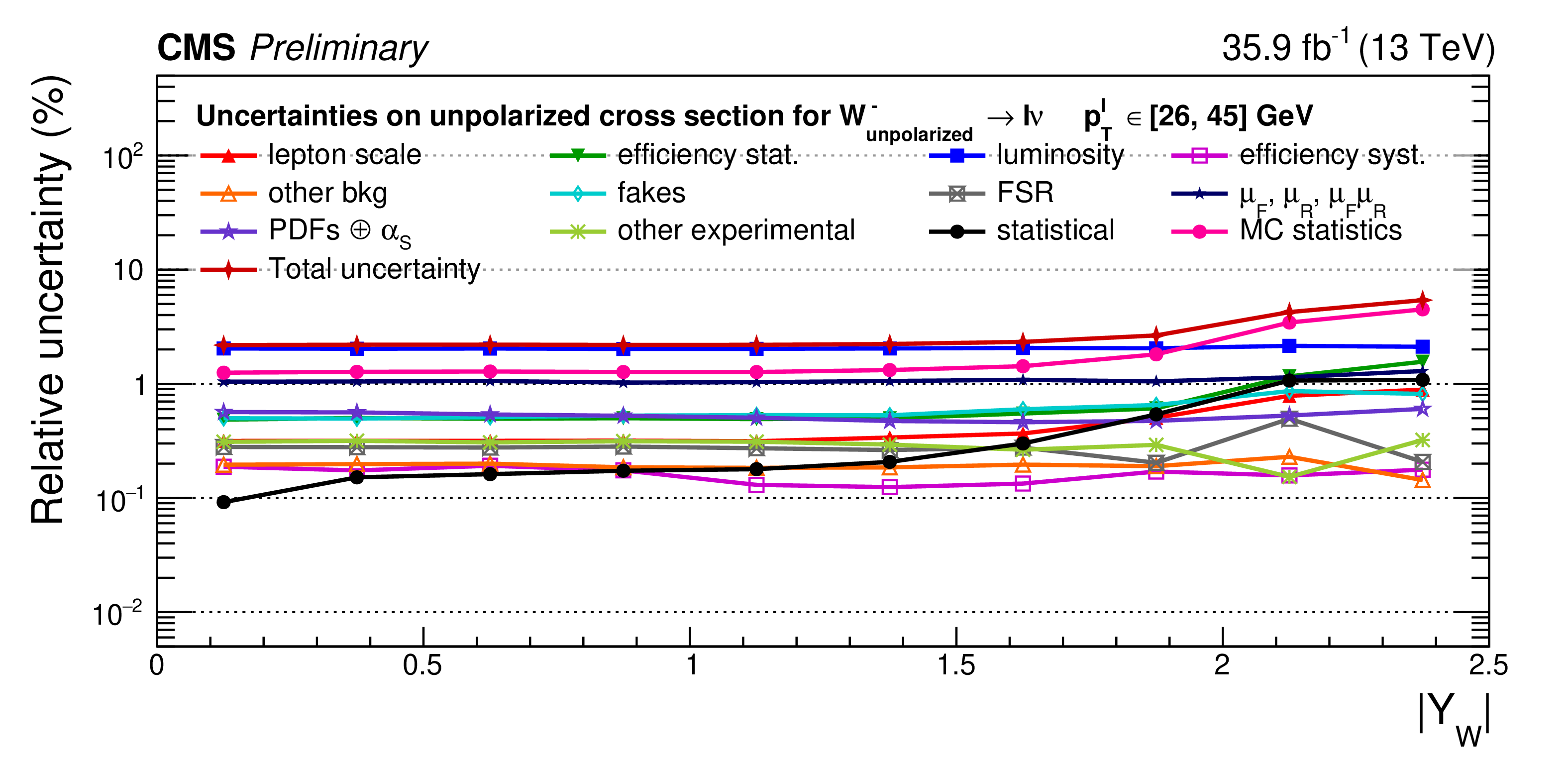
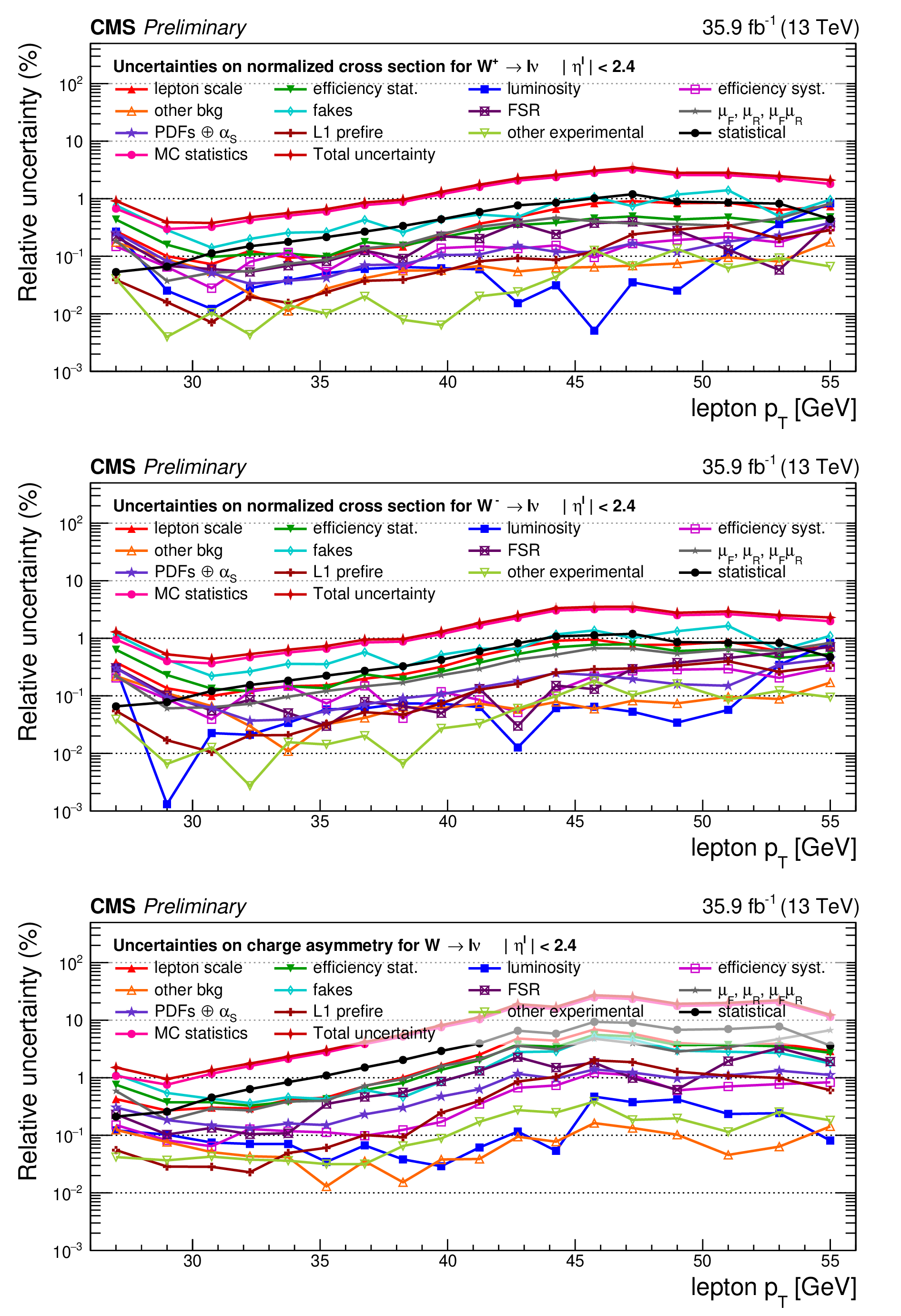
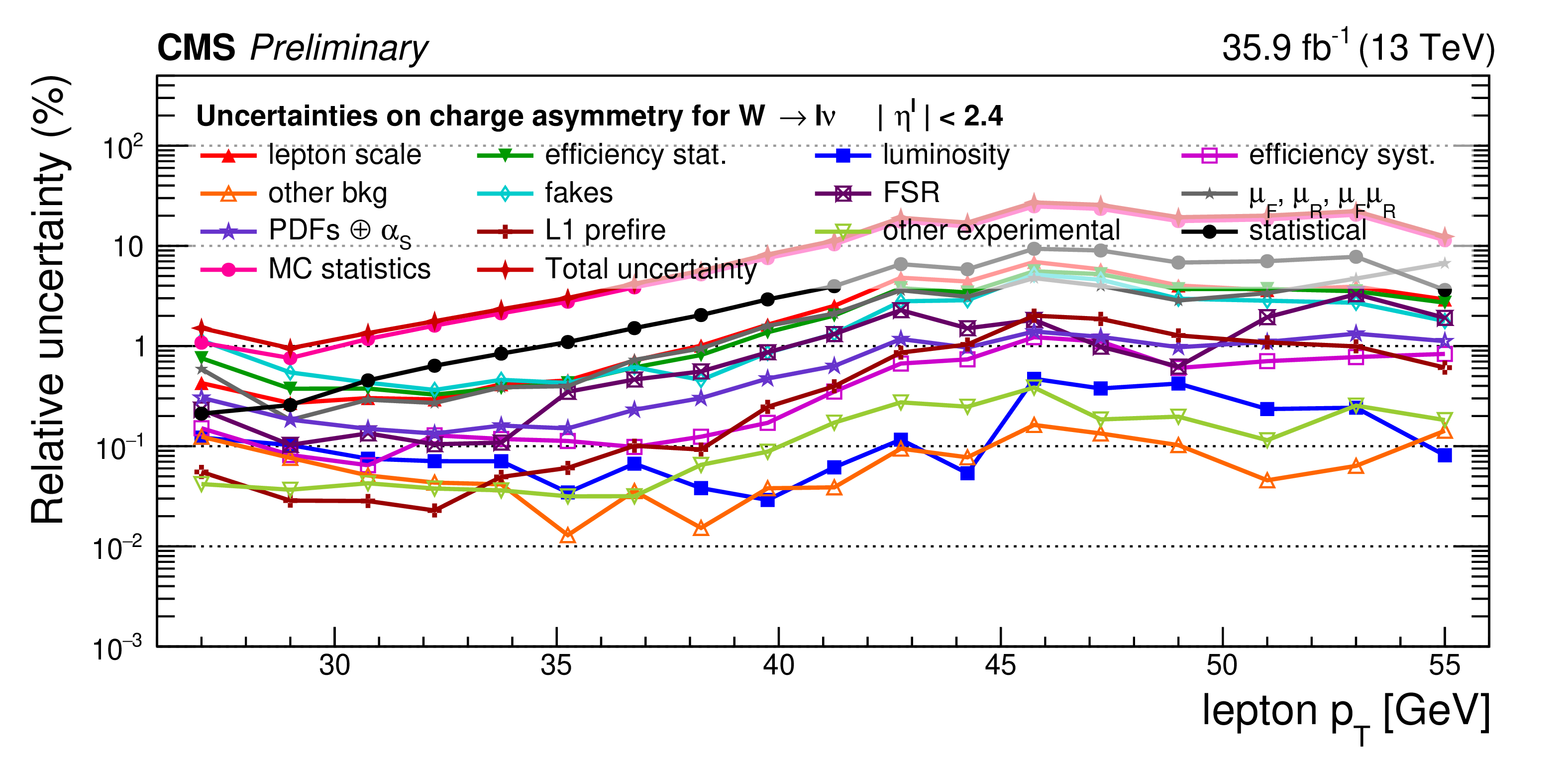
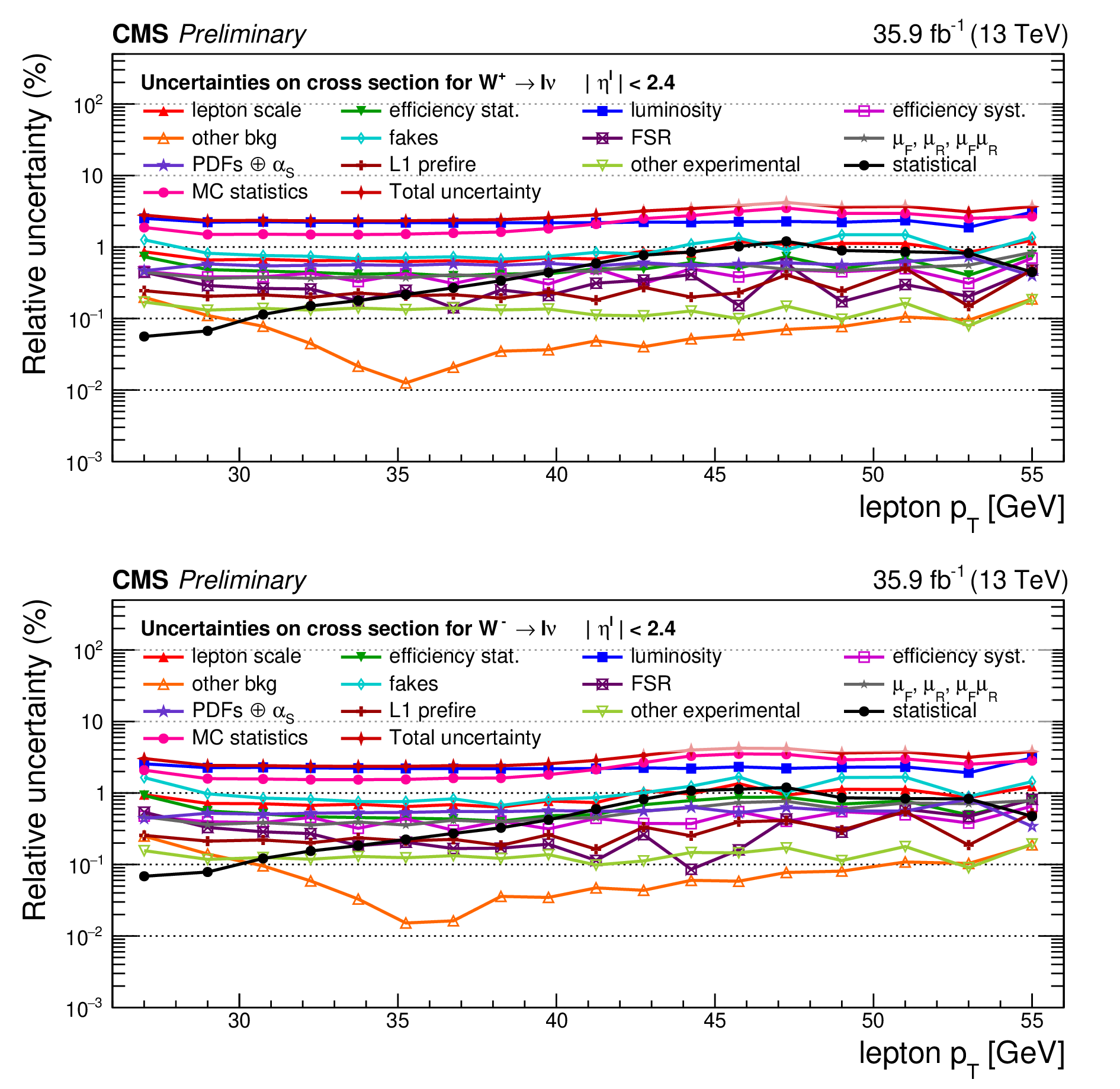
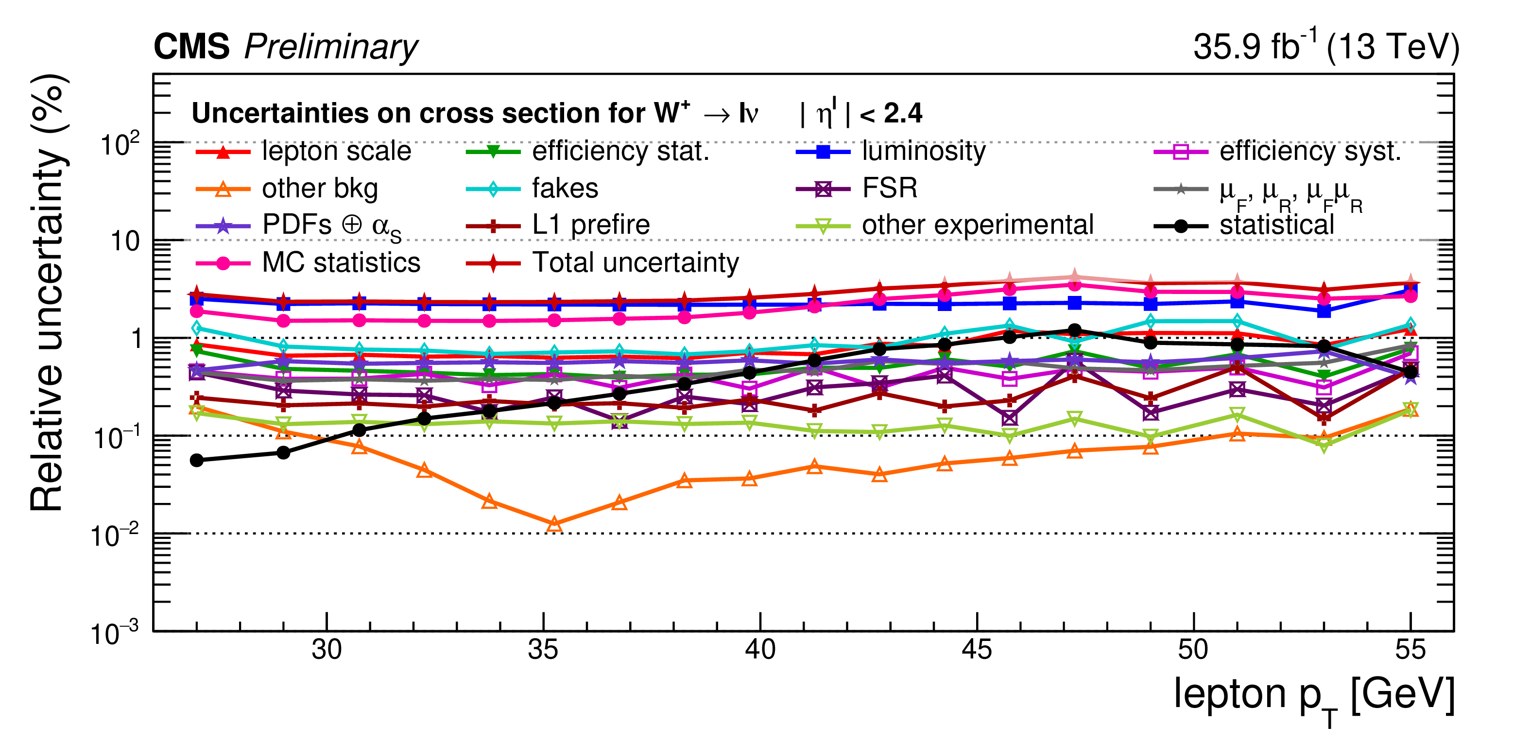
Figure 4:
Top: relative impact of groups of systematic uncertainties (as defined in the text) on the signal normalized cross sections for the $ {\mathrm{W^{+}}} $ case. Bottom: relative impact of uncertainties on charge asymmetry (bottom). All impacts are shown for the combination of the muon and electron channels. |
png pdf |
Figure 4-a:
Top: relative impact of groups of systematic uncertainties (as defined in the text) on the signal normalized cross sections for the $ {\mathrm{W^{+}}} $ case. Bottom: relative impact of uncertainties on charge asymmetry (bottom). All impacts are shown for the combination of the muon and electron channels. |
png pdf |
Figure 4-b:
Top: relative impact of groups of systematic uncertainties (as defined in the text) on the signal normalized cross sections for the $ {\mathrm{W^{+}}} $ case. Bottom: relative impact of uncertainties on charge asymmetry (bottom). All impacts are shown for the combination of the muon and electron channels. |

png pdf |
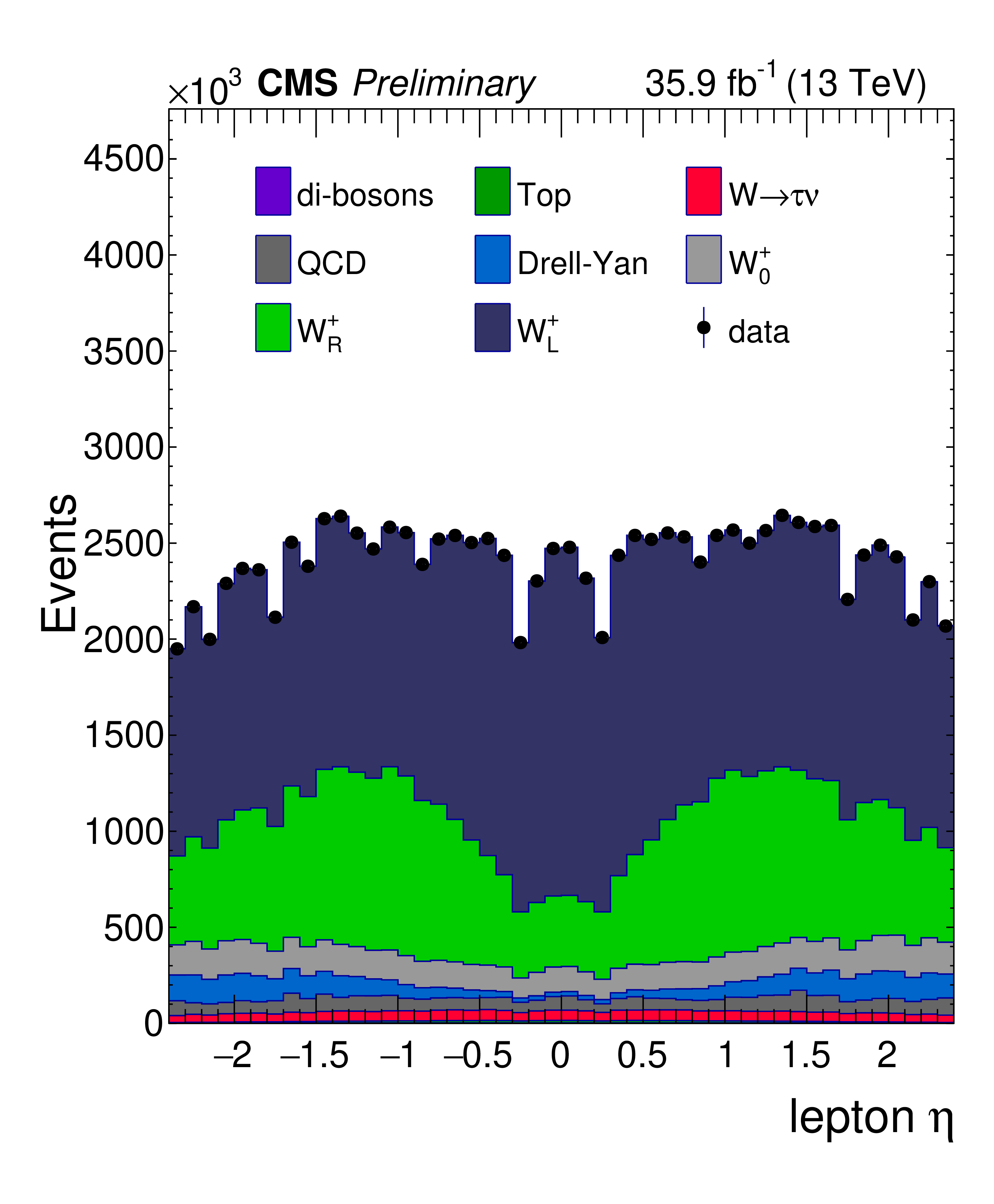
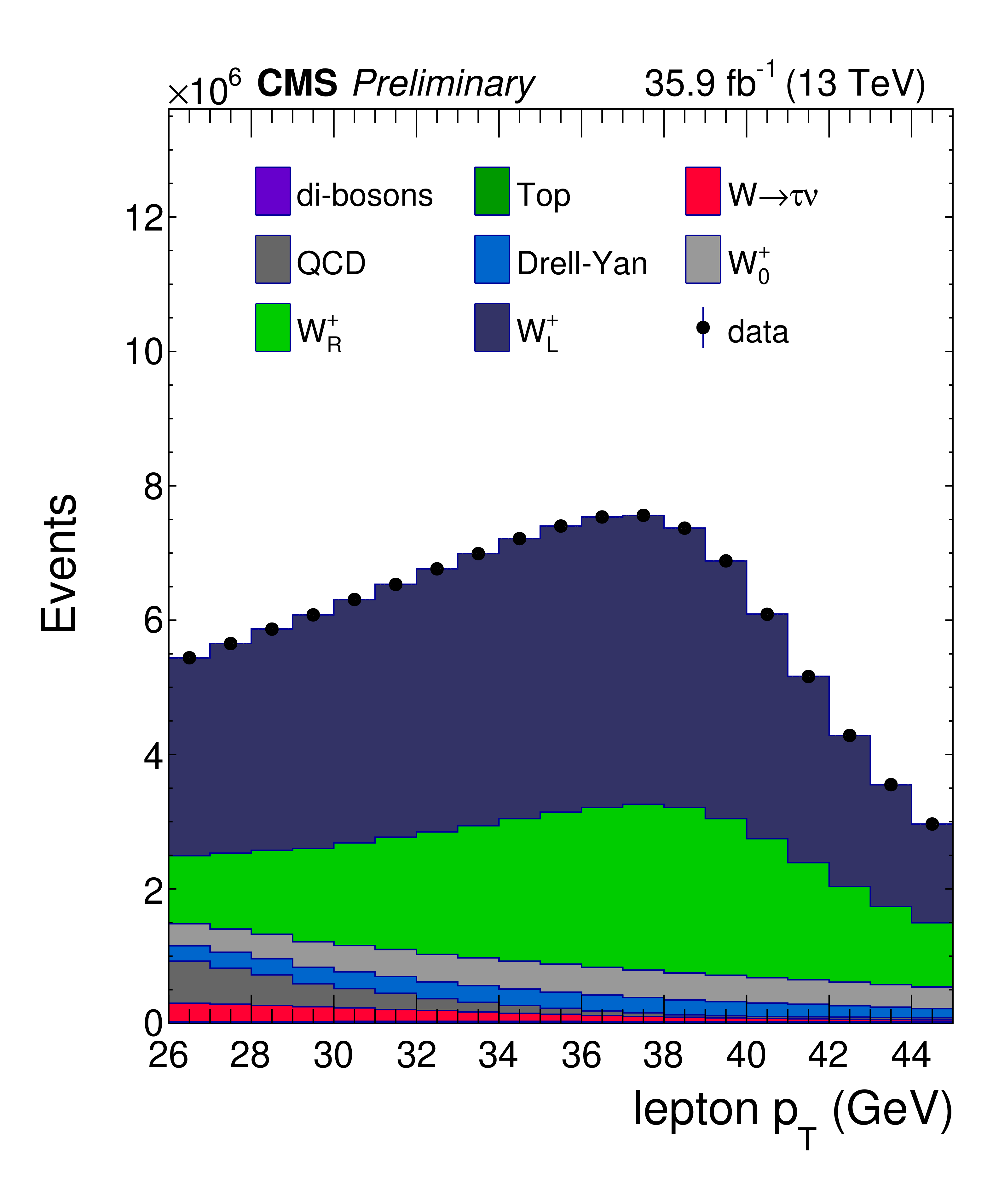
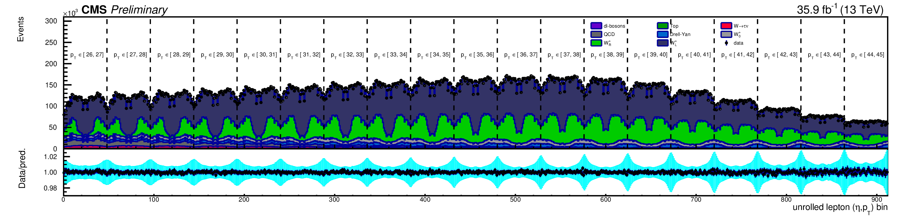
Figure 5:
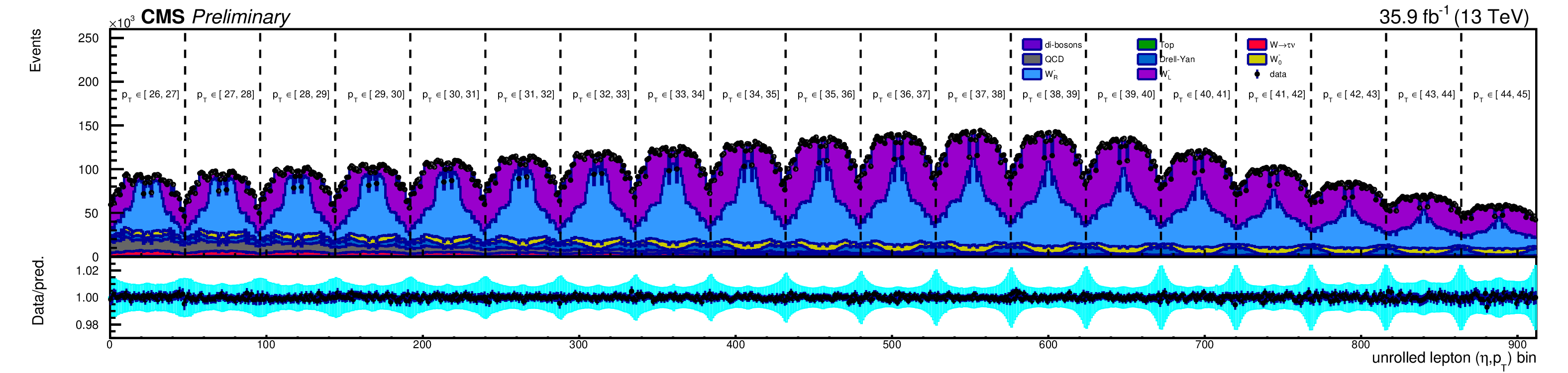
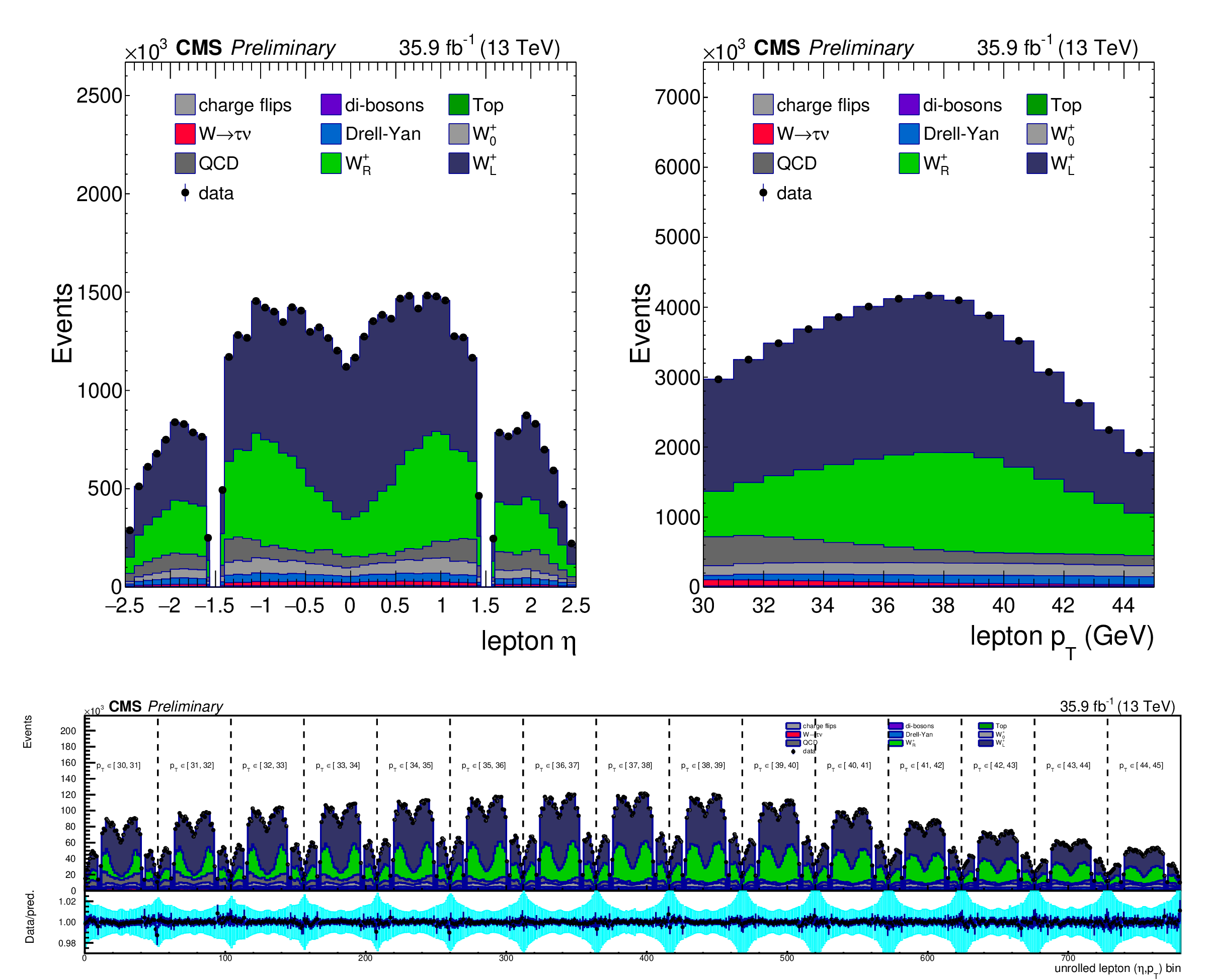
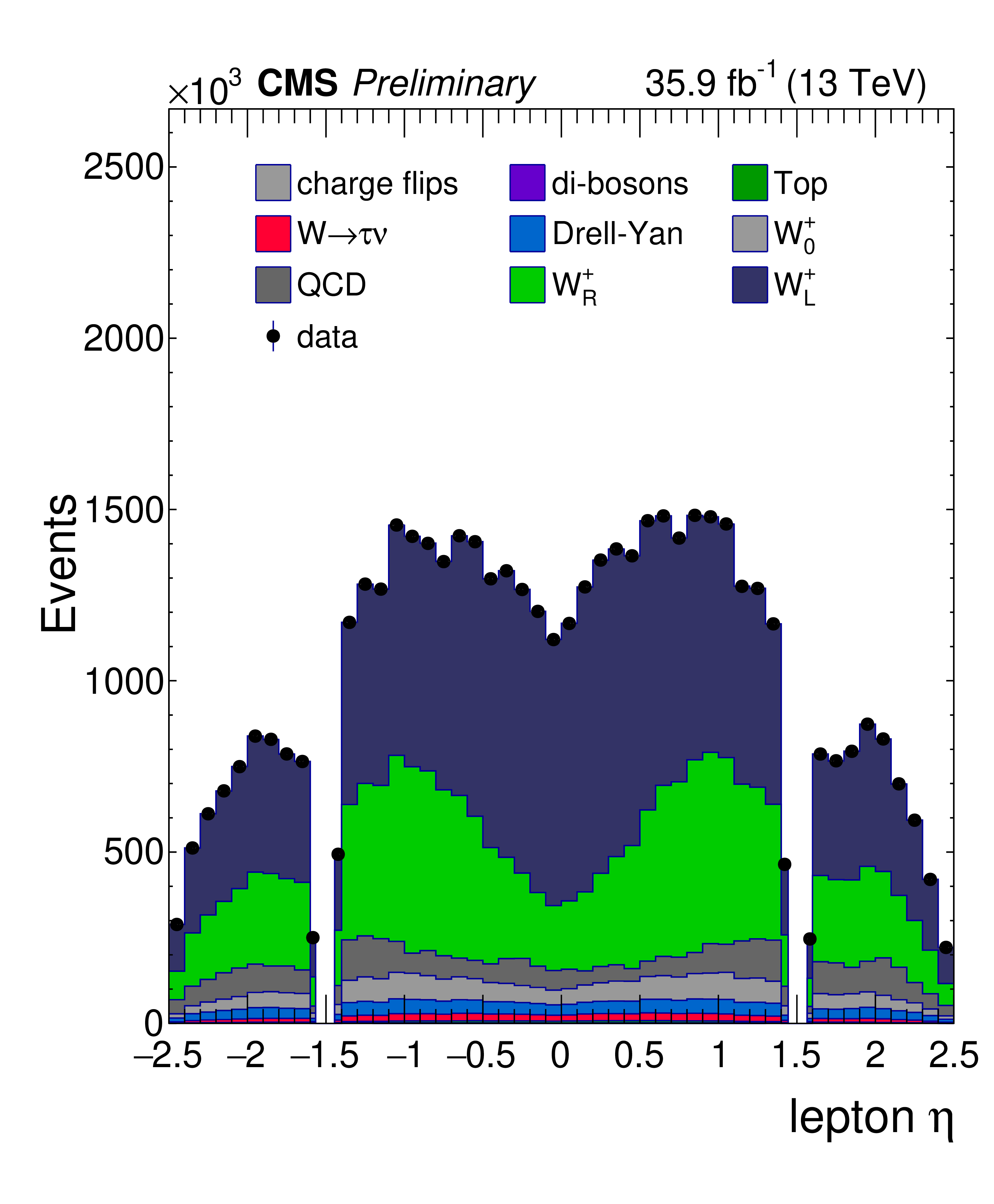
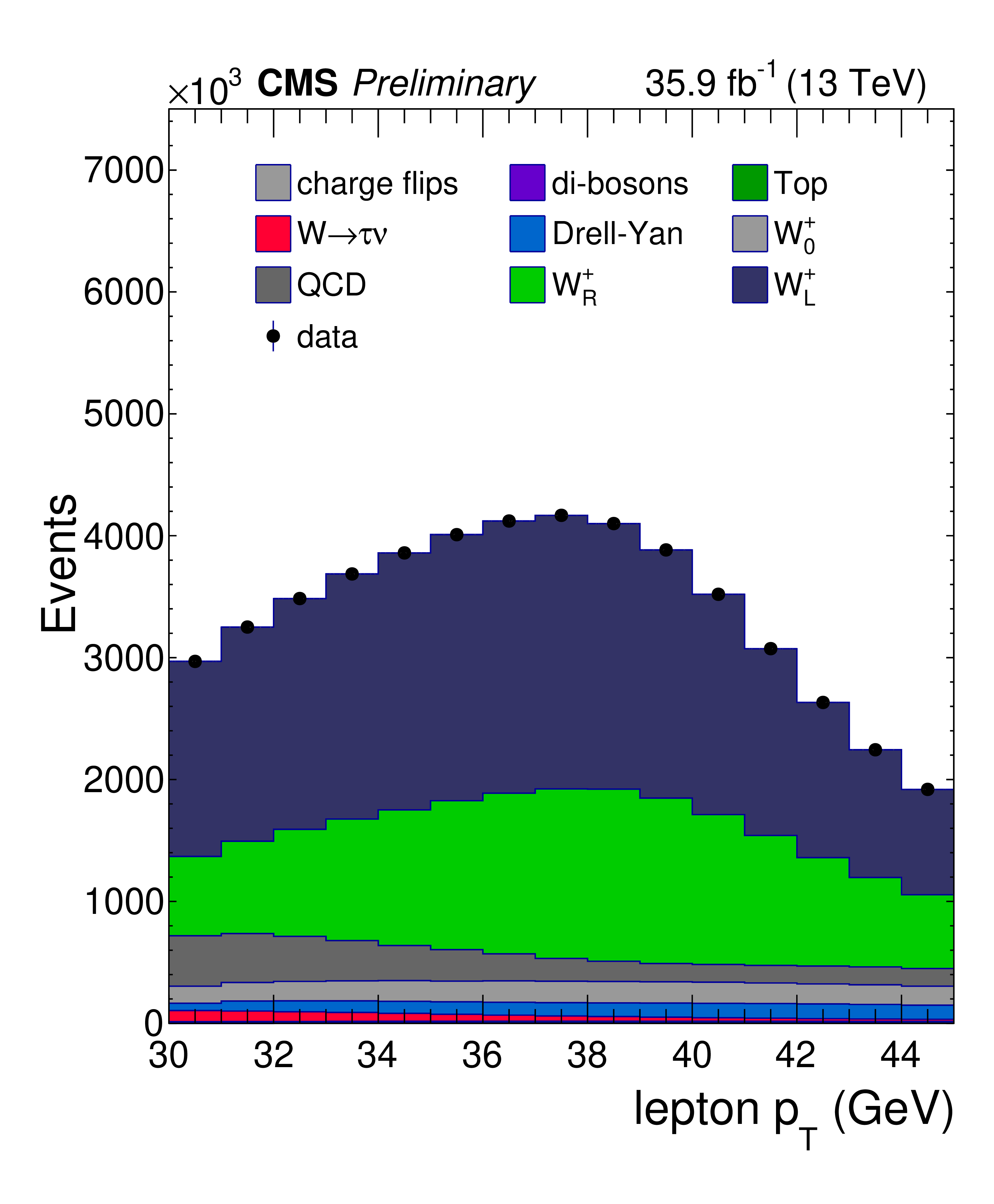
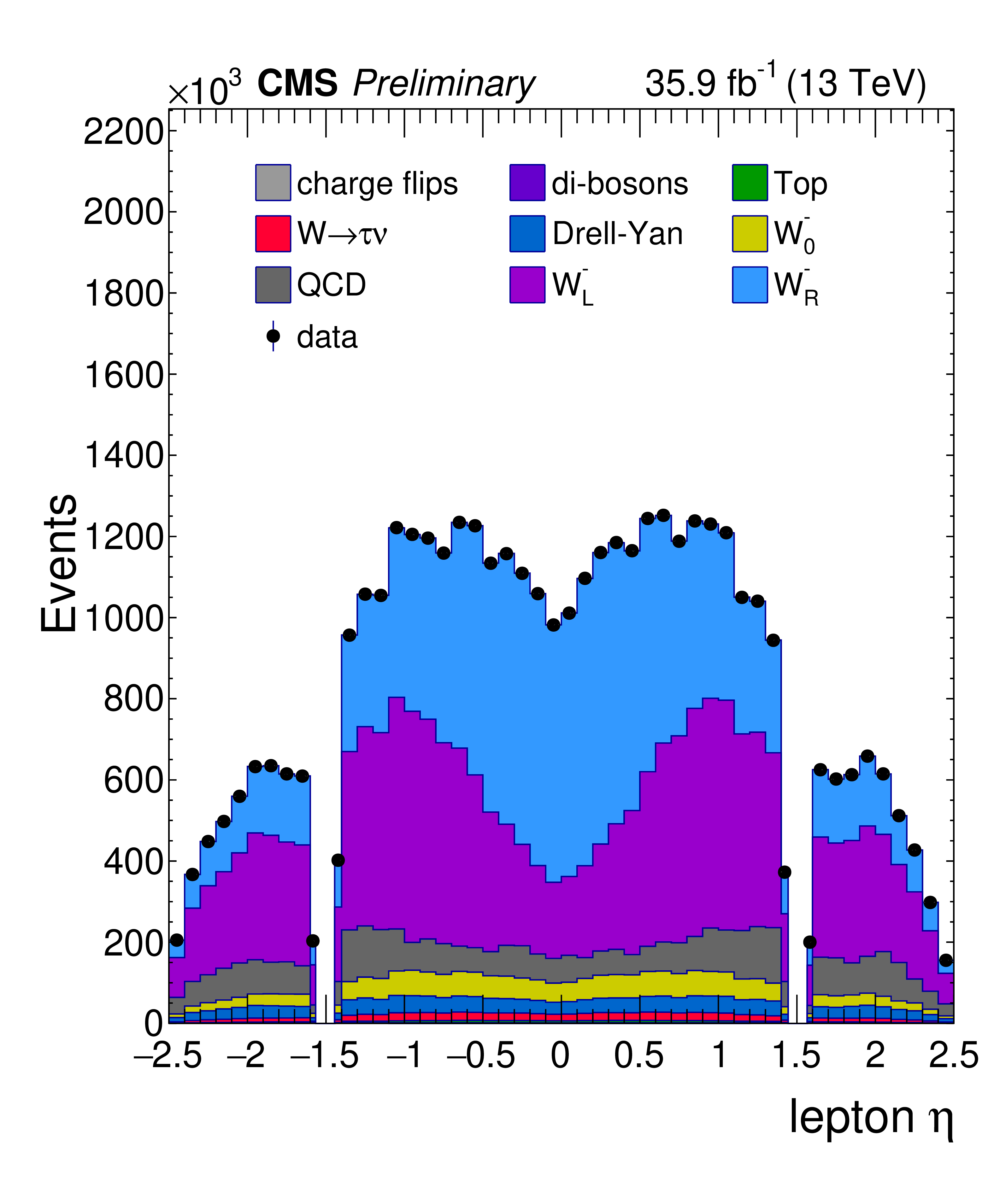
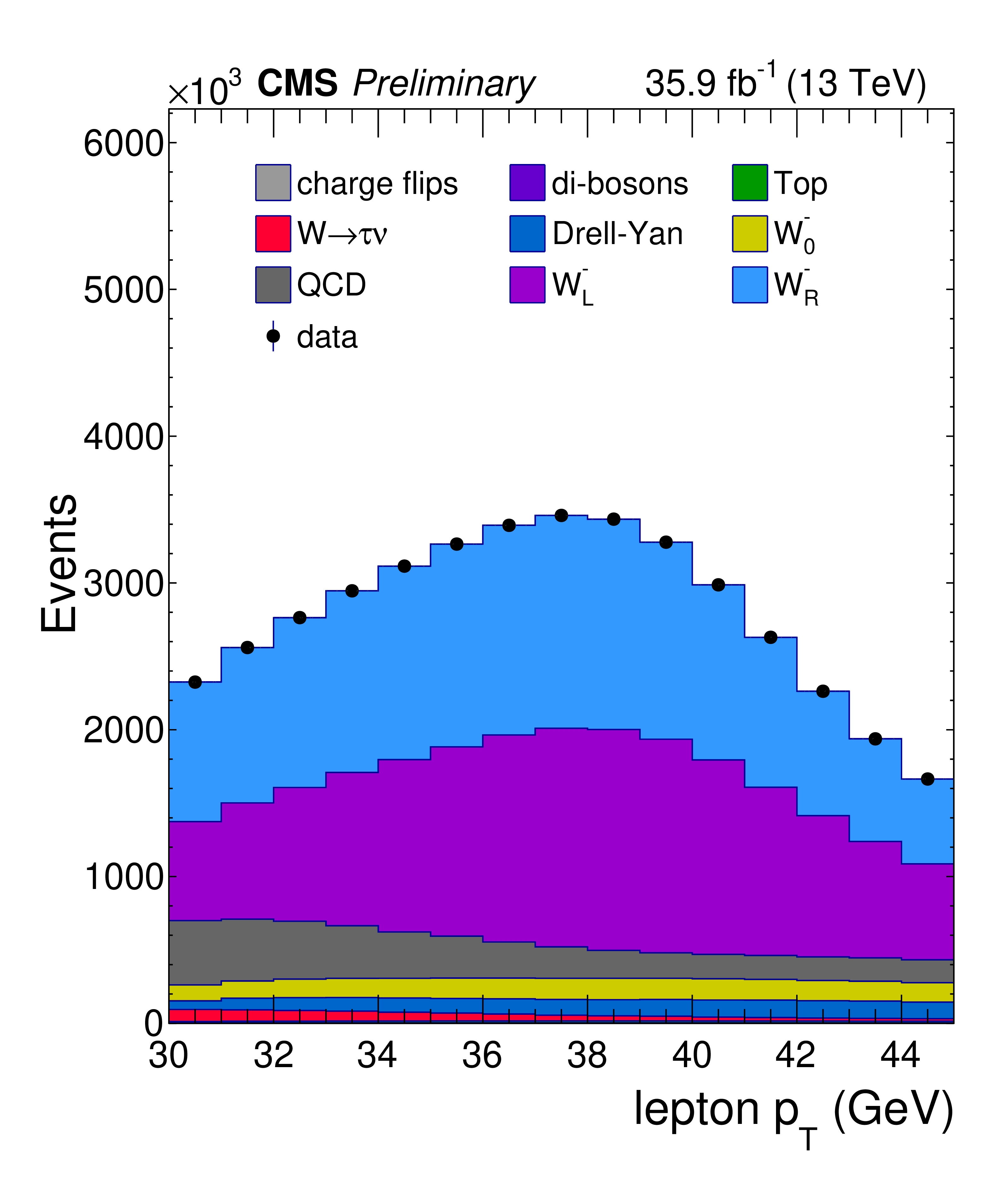
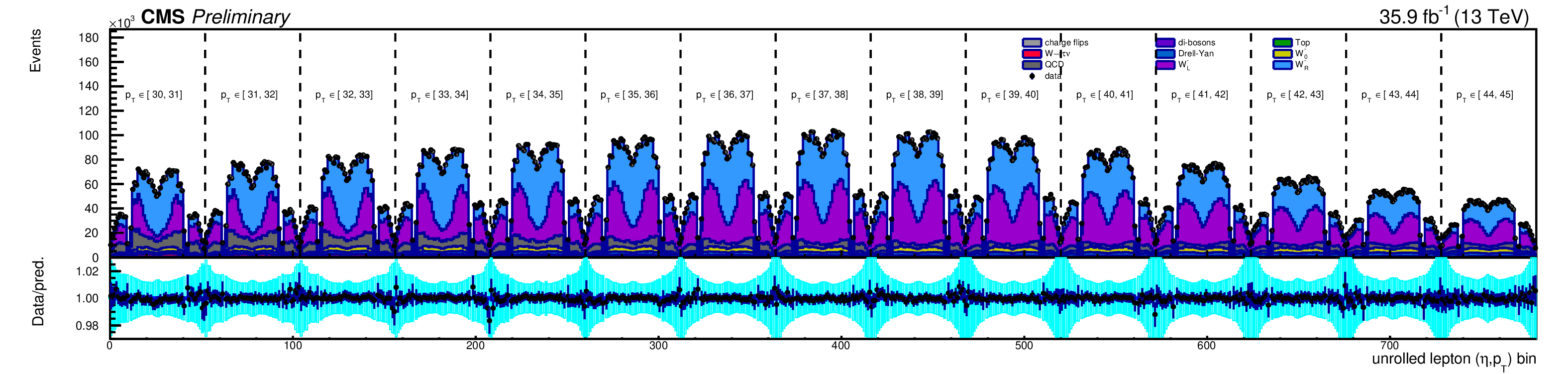
Distributions of ${\eta ^{\, \mu}}$ (a), ${{p_{\mathrm {T}}} ^{\, \mu}}$ (b) and bin$_{{\text{unrolled}}}$ (c) for $ {\mathrm{W^{+}}} \to \mu ^+\nu $ events for observed data superimposed on signal plus background events. The signal and background processes are normalized to the result of the template fit. The cyan band over the data-to-prediction ratio represents the uncertainty in the yield in each bin after the profiling process. |
png pdf |
Figure 5-a:
Distributions of ${\eta ^{\, \mu}}$ (a), ${{p_{\mathrm {T}}} ^{\, \mu}}$ (b) and bin$_{{\text{unrolled}}}$ (c) for $ {\mathrm{W^{+}}} \to \mu ^+\nu $ events for observed data superimposed on signal plus background events. The signal and background processes are normalized to the result of the template fit. The cyan band over the data-to-prediction ratio represents the uncertainty in the yield in each bin after the profiling process. |
png pdf |
Figure 5-b:
Distributions of ${\eta ^{\, \mu}}$ (a), ${{p_{\mathrm {T}}} ^{\, \mu}}$ (b) and bin$_{{\text{unrolled}}}$ (c) for $ {\mathrm{W^{+}}} \to \mu ^+\nu $ events for observed data superimposed on signal plus background events. The signal and background processes are normalized to the result of the template fit. The cyan band over the data-to-prediction ratio represents the uncertainty in the yield in each bin after the profiling process. |
png pdf |
Figure 5-c:
Distributions of ${\eta ^{\, \mu}}$ (a), ${{p_{\mathrm {T}}} ^{\, \mu}}$ (b) and bin$_{{\text{unrolled}}}$ (c) for $ {\mathrm{W^{+}}} \to \mu ^+\nu $ events for observed data superimposed on signal plus background events. The signal and background processes are normalized to the result of the template fit. The cyan band over the data-to-prediction ratio represents the uncertainty in the yield in each bin after the profiling process. |
png pdf |
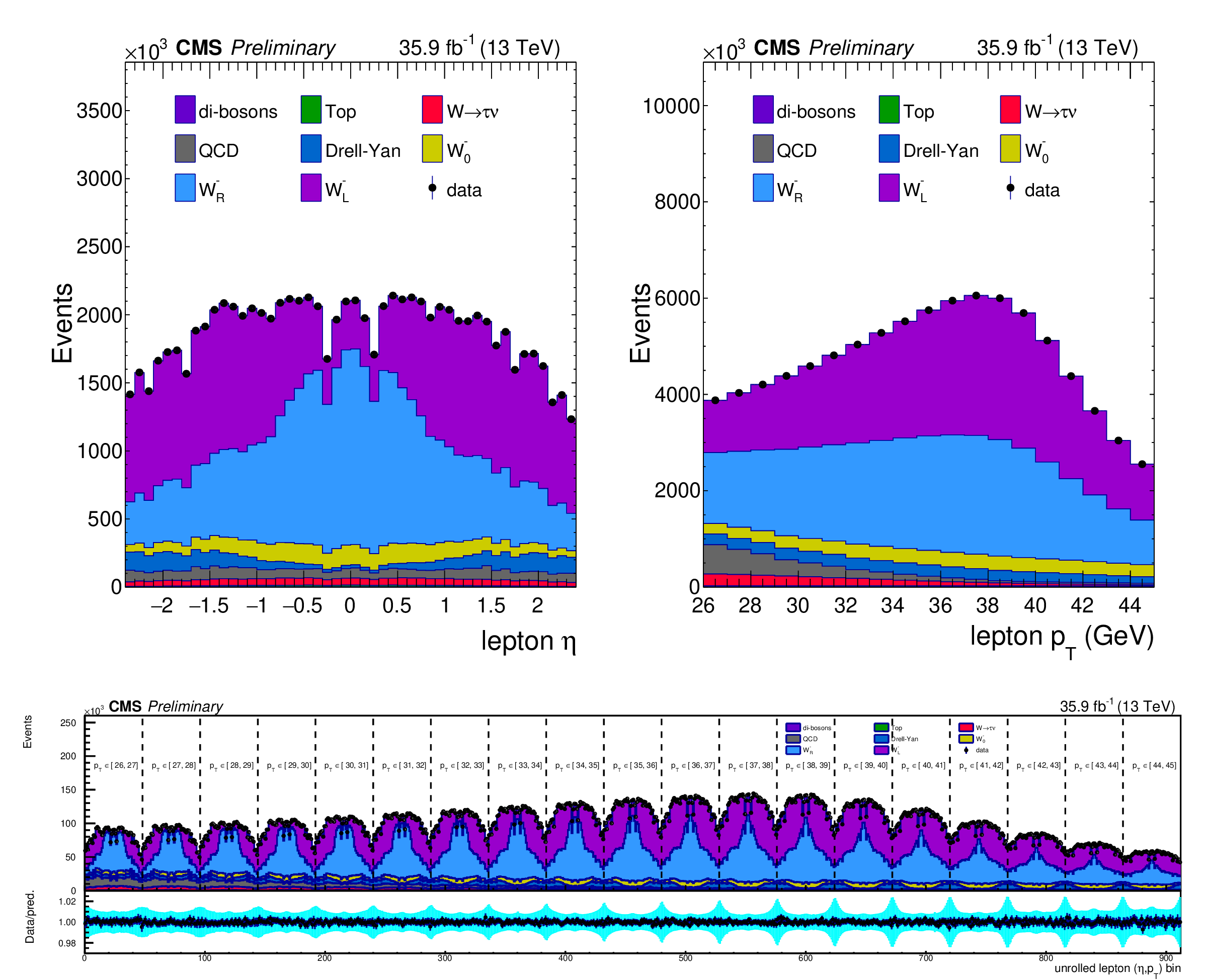
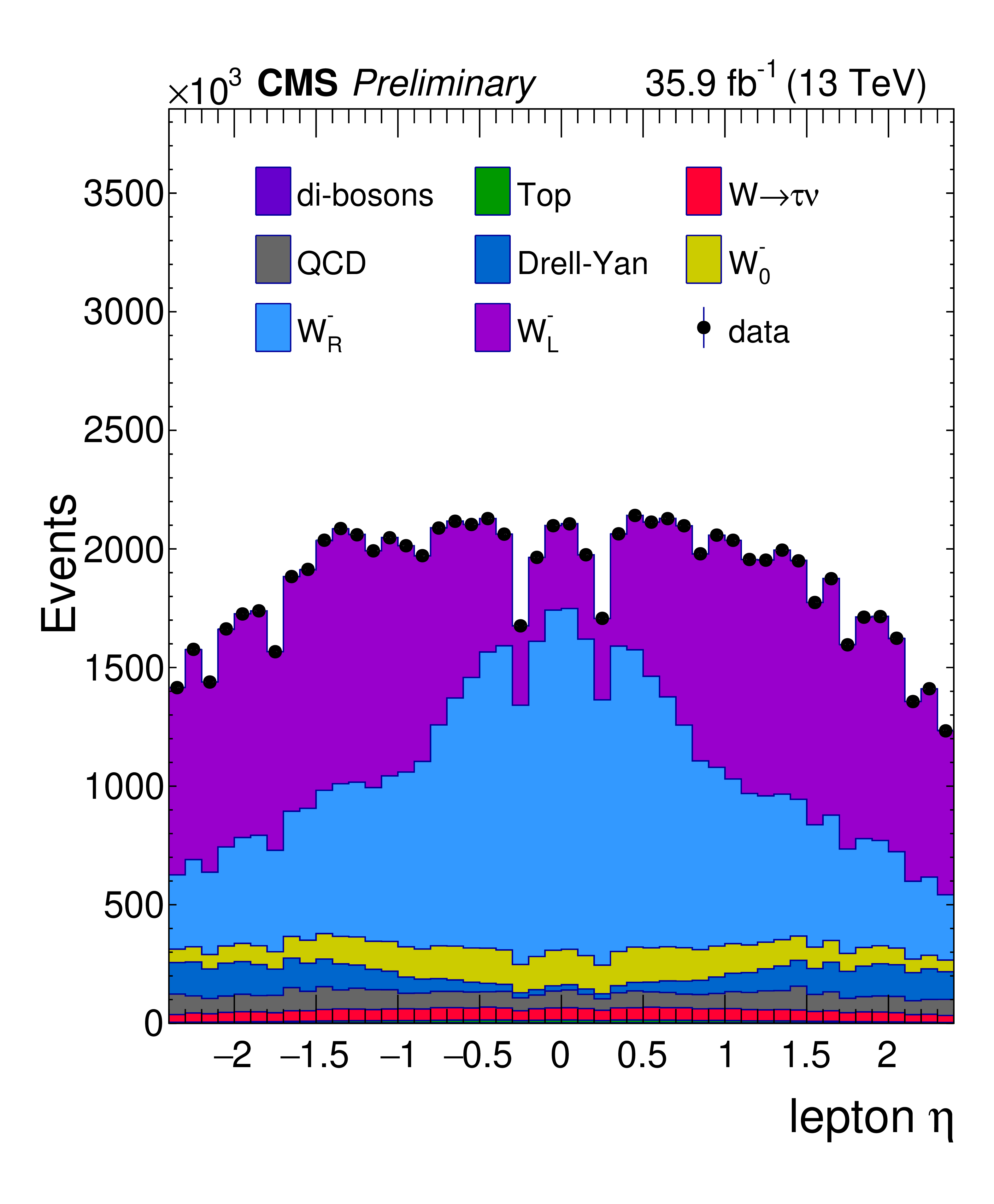
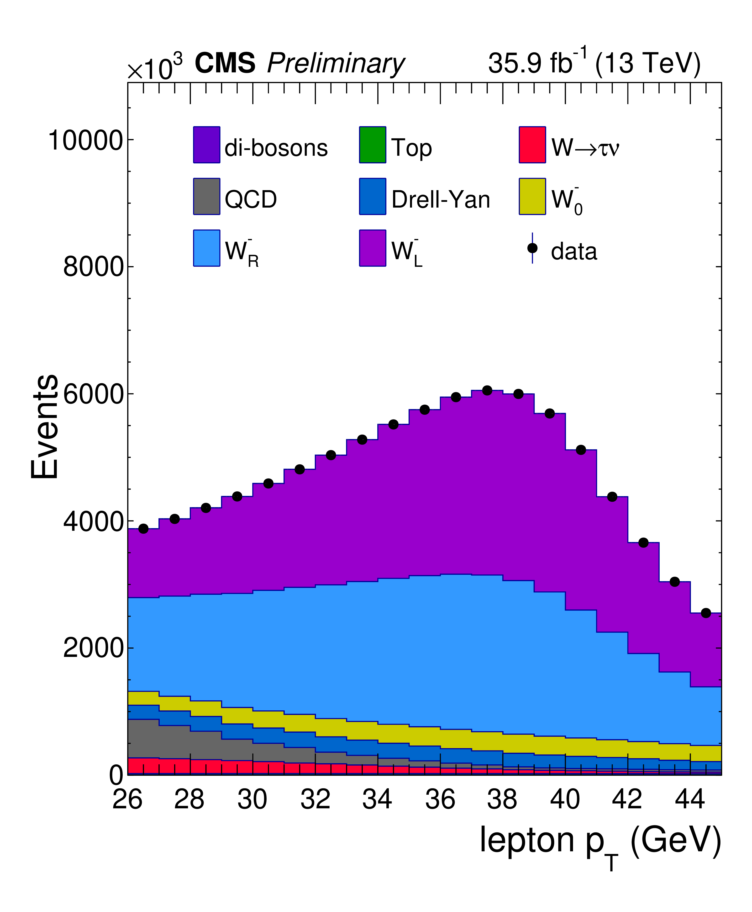
Figure 6:
Distributions of ${\eta ^{\, \mu}}$ (a), ${{p_{\mathrm {T}}} ^{\, \mu}}$ (b) and bin$_{{\text{unrolled}}}$ (c) for $ {\mathrm{W^{-}}} \to \mu ^-\bar\nu $ events for observed data superimposed on signal plus background events. The signal and background processes are normalized to the result of the template fit. The cyan band over the data-to-prediction ratio represents the uncertainty in the yield in each bin after the profiling process. |
png pdf |
Figure 6-a:
Distributions of ${\eta ^{\, \mu}}$ (a), ${{p_{\mathrm {T}}} ^{\, \mu}}$ (b) and bin$_{{\text{unrolled}}}$ (c) for $ {\mathrm{W^{-}}} \to \mu ^-\bar\nu $ events for observed data superimposed on signal plus background events. The signal and background processes are normalized to the result of the template fit. The cyan band over the data-to-prediction ratio represents the uncertainty in the yield in each bin after the profiling process. |
png pdf |
Figure 6-b:
Distributions of ${\eta ^{\, \mu}}$ (a), ${{p_{\mathrm {T}}} ^{\, \mu}}$ (b) and bin$_{{\text{unrolled}}}$ (c) for $ {\mathrm{W^{-}}} \to \mu ^-\bar\nu $ events for observed data superimposed on signal plus background events. The signal and background processes are normalized to the result of the template fit. The cyan band over the data-to-prediction ratio represents the uncertainty in the yield in each bin after the profiling process. |
png pdf |
Figure 6-c:
Distributions of ${\eta ^{\, \mu}}$ (a), ${{p_{\mathrm {T}}} ^{\, \mu}}$ (b) and bin$_{{\text{unrolled}}}$ (c) for $ {\mathrm{W^{-}}} \to \mu ^-\bar\nu $ events for observed data superimposed on signal plus background events. The signal and background processes are normalized to the result of the template fit. The cyan band over the data-to-prediction ratio represents the uncertainty in the yield in each bin after the profiling process. |
png pdf |
Figure 7:
Distributions of ${\eta ^{\mathrm{e}}}$ (a), ${{p_{\mathrm {T}}} ^{\mathrm{e}}}$ (b) and bin$_{{\text{unrolled}}}$ (c) for $ {\mathrm{W^{+}}} \to \mathrm{e} ^+\nu $ events for observed data superimposed on signal plus background events. The signal and background processes are normalized to the result of the template fit. The cyan band over the data-to-prediction ratio represents the uncertainty in the yield in each bin after the profiling process. |
png pdf |
Figure 7-a:
Distributions of ${\eta ^{\mathrm{e}}}$ (a), ${{p_{\mathrm {T}}} ^{\mathrm{e}}}$ (b) and bin$_{{\text{unrolled}}}$ (c) for $ {\mathrm{W^{+}}} \to \mathrm{e} ^+\nu $ events for observed data superimposed on signal plus background events. The signal and background processes are normalized to the result of the template fit. The cyan band over the data-to-prediction ratio represents the uncertainty in the yield in each bin after the profiling process. |
png pdf |
Figure 7-b:
Distributions of ${\eta ^{\mathrm{e}}}$ (a), ${{p_{\mathrm {T}}} ^{\mathrm{e}}}$ (b) and bin$_{{\text{unrolled}}}$ (c) for $ {\mathrm{W^{+}}} \to \mathrm{e} ^+\nu $ events for observed data superimposed on signal plus background events. The signal and background processes are normalized to the result of the template fit. The cyan band over the data-to-prediction ratio represents the uncertainty in the yield in each bin after the profiling process. |

png pdf |
Figure 7-c:
Distributions of ${\eta ^{\mathrm{e}}}$ (a), ${{p_{\mathrm {T}}} ^{\mathrm{e}}}$ (b) and bin$_{{\text{unrolled}}}$ (c) for $ {\mathrm{W^{+}}} \to \mathrm{e} ^+\nu $ events for observed data superimposed on signal plus background events. The signal and background processes are normalized to the result of the template fit. The cyan band over the data-to-prediction ratio represents the uncertainty in the yield in each bin after the profiling process. |

png pdf |
Figure 8:
Distributions of ${\eta ^{\mathrm{e}}}$ (a), ${{p_{\mathrm {T}}} ^{\mathrm{e}}}$ (b) and bin$_{{\text{unrolled}}}$ (c) for $ {\mathrm{W^{-}}} \to \mathrm{e} ^-\bar\nu $ events for observed data superimposed on signal plus background events. The signal and background processes are normalized to the result of the template fit. The cyan band over the data-to-prediction ratio represents the uncertainty in the yield in each bin after the profiling process. |
png pdf |
Figure 8-a:
Distributions of ${\eta ^{\mathrm{e}}}$ (a), ${{p_{\mathrm {T}}} ^{\mathrm{e}}}$ (b) and bin$_{{\text{unrolled}}}$ (c) for $ {\mathrm{W^{-}}} \to \mathrm{e} ^-\bar\nu $ events for observed data superimposed on signal plus background events. The signal and background processes are normalized to the result of the template fit. The cyan band over the data-to-prediction ratio represents the uncertainty in the yield in each bin after the profiling process. |
png pdf |
Figure 8-b:
Distributions of ${\eta ^{\mathrm{e}}}$ (a), ${{p_{\mathrm {T}}} ^{\mathrm{e}}}$ (b) and bin$_{{\text{unrolled}}}$ (c) for $ {\mathrm{W^{-}}} \to \mathrm{e} ^-\bar\nu $ events for observed data superimposed on signal plus background events. The signal and background processes are normalized to the result of the template fit. The cyan band over the data-to-prediction ratio represents the uncertainty in the yield in each bin after the profiling process. |
png pdf |
Figure 8-c:
Distributions of ${\eta ^{\mathrm{e}}}$ (a), ${{p_{\mathrm {T}}} ^{\mathrm{e}}}$ (b) and bin$_{{\text{unrolled}}}$ (c) for $ {\mathrm{W^{-}}} \to \mathrm{e} ^-\bar\nu $ events for observed data superimposed on signal plus background events. The signal and background processes are normalized to the result of the template fit. The cyan band over the data-to-prediction ratio represents the uncertainty in the yield in each bin after the profiling process. |
png pdf |
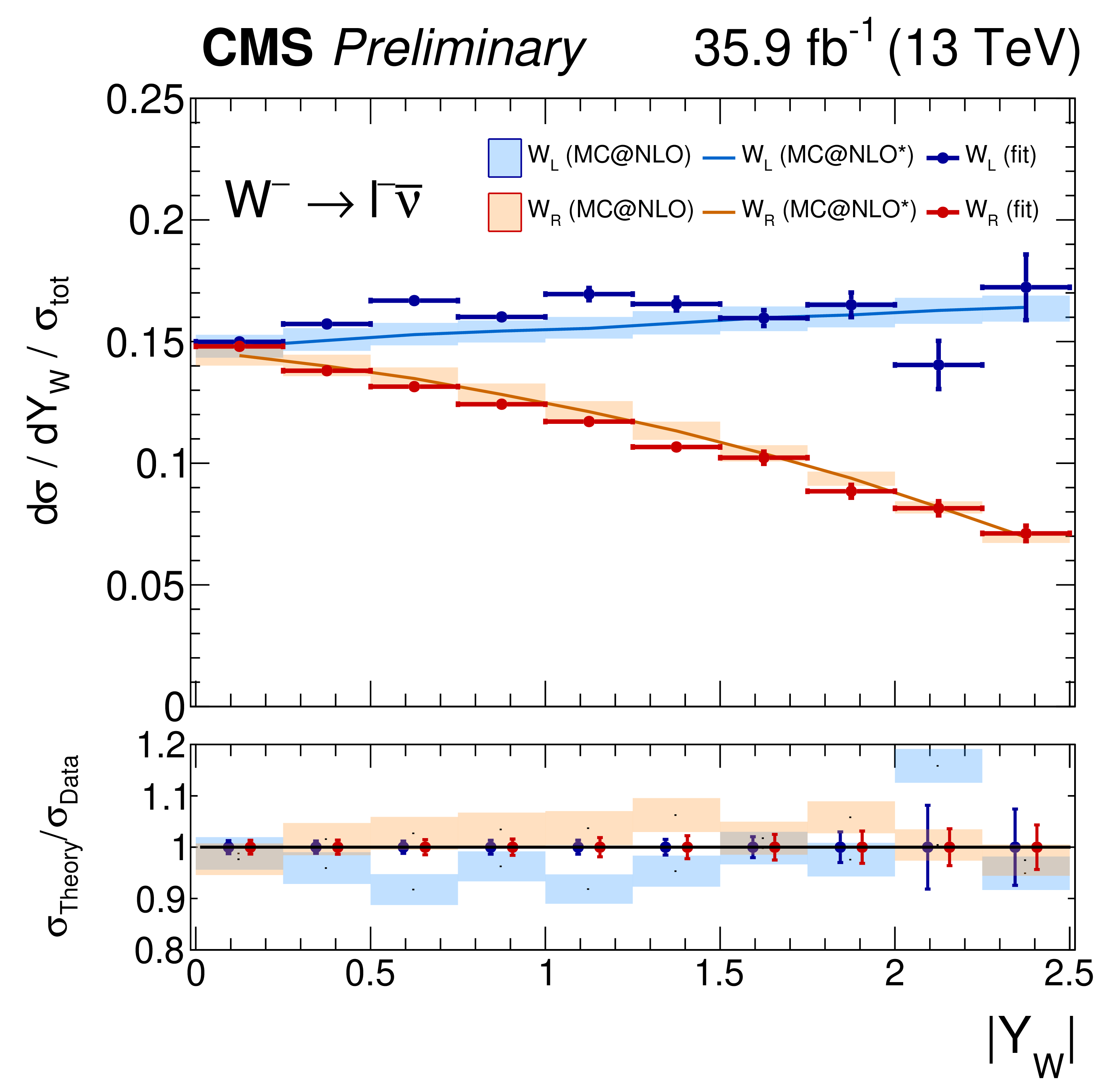
Figure 9:
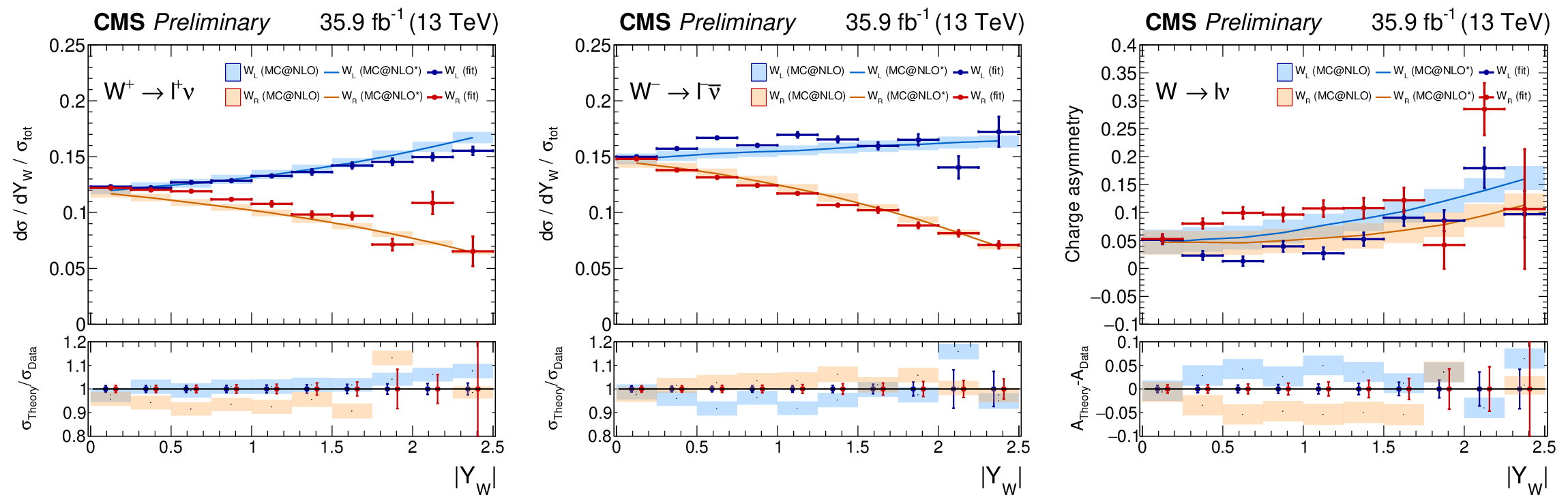
Measured normalized $\mathrm{W} \to \ell ^+\nu $ (left) or $\mathrm{W} \to \ell ^-\bar\nu $ (middle) cross section as a function of $ {| Y_{\mathrm{W}} |} $ for the left-handed and right-handed helicity states from the combination of muon and electron channels, normalized to the total cross section. Right: measured W charge asymmetry. Also shown is the ratio of the prediction from MadGraph 5_aMC@NLO to the data. The light-filled band corresponds to the expected uncertainty from the PDF variations, QCD scales and $\alpha _S$. |

png pdf |
Figure 9-a:
Measured normalized $\mathrm{W} \to \ell ^+\nu $ (left) or $\mathrm{W} \to \ell ^-\bar\nu $ (middle) cross section as a function of $ {| Y_{\mathrm{W}} |} $ for the left-handed and right-handed helicity states from the combination of muon and electron channels, normalized to the total cross section. Right: measured W charge asymmetry. Also shown is the ratio of the prediction from MadGraph 5_aMC@NLO to the data. The light-filled band corresponds to the expected uncertainty from the PDF variations, QCD scales and $\alpha _S$. |
png pdf |
Figure 9-b:
Measured normalized $\mathrm{W} \to \ell ^+\nu $ (left) or $\mathrm{W} \to \ell ^-\bar\nu $ (middle) cross section as a function of $ {| Y_{\mathrm{W}} |} $ for the left-handed and right-handed helicity states from the combination of muon and electron channels, normalized to the total cross section. Right: measured W charge asymmetry. Also shown is the ratio of the prediction from MadGraph 5_aMC@NLO to the data. The light-filled band corresponds to the expected uncertainty from the PDF variations, QCD scales and $\alpha _S$. |

png pdf |
Figure 9-c:
Measured normalized $\mathrm{W} \to \ell ^+\nu $ (left) or $\mathrm{W} \to \ell ^-\bar\nu $ (middle) cross section as a function of $ {| Y_{\mathrm{W}} |} $ for the left-handed and right-handed helicity states from the combination of muon and electron channels, normalized to the total cross section. Right: measured W charge asymmetry. Also shown is the ratio of the prediction from MadGraph 5_aMC@NLO to the data. The light-filled band corresponds to the expected uncertainty from the PDF variations, QCD scales and $\alpha _S$. |

png pdf |
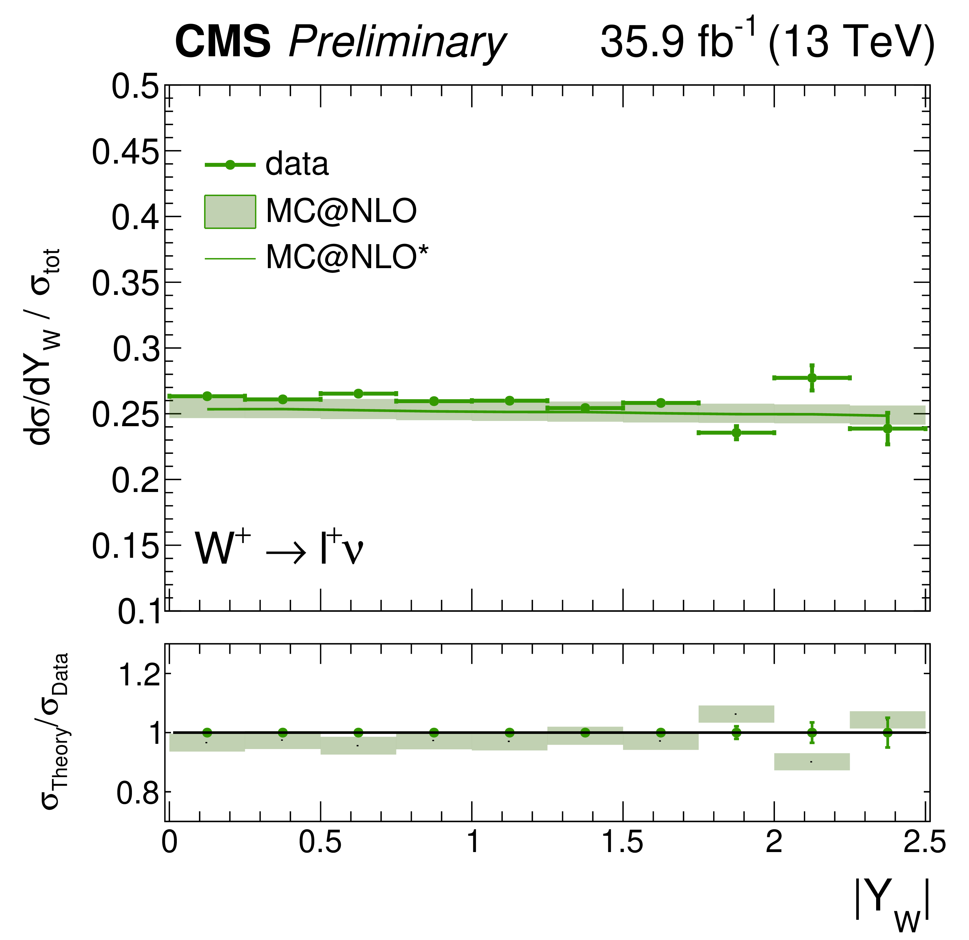
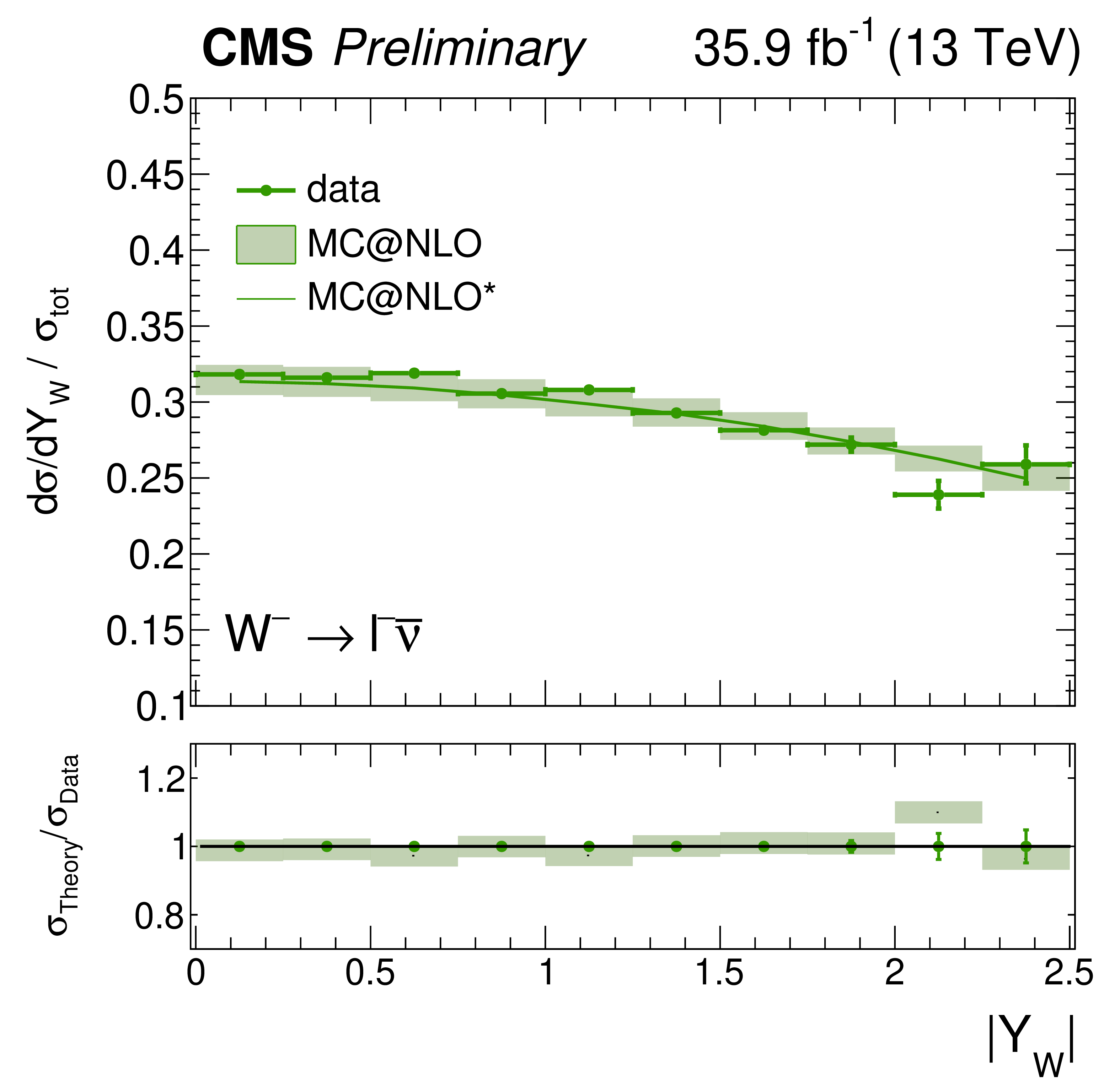
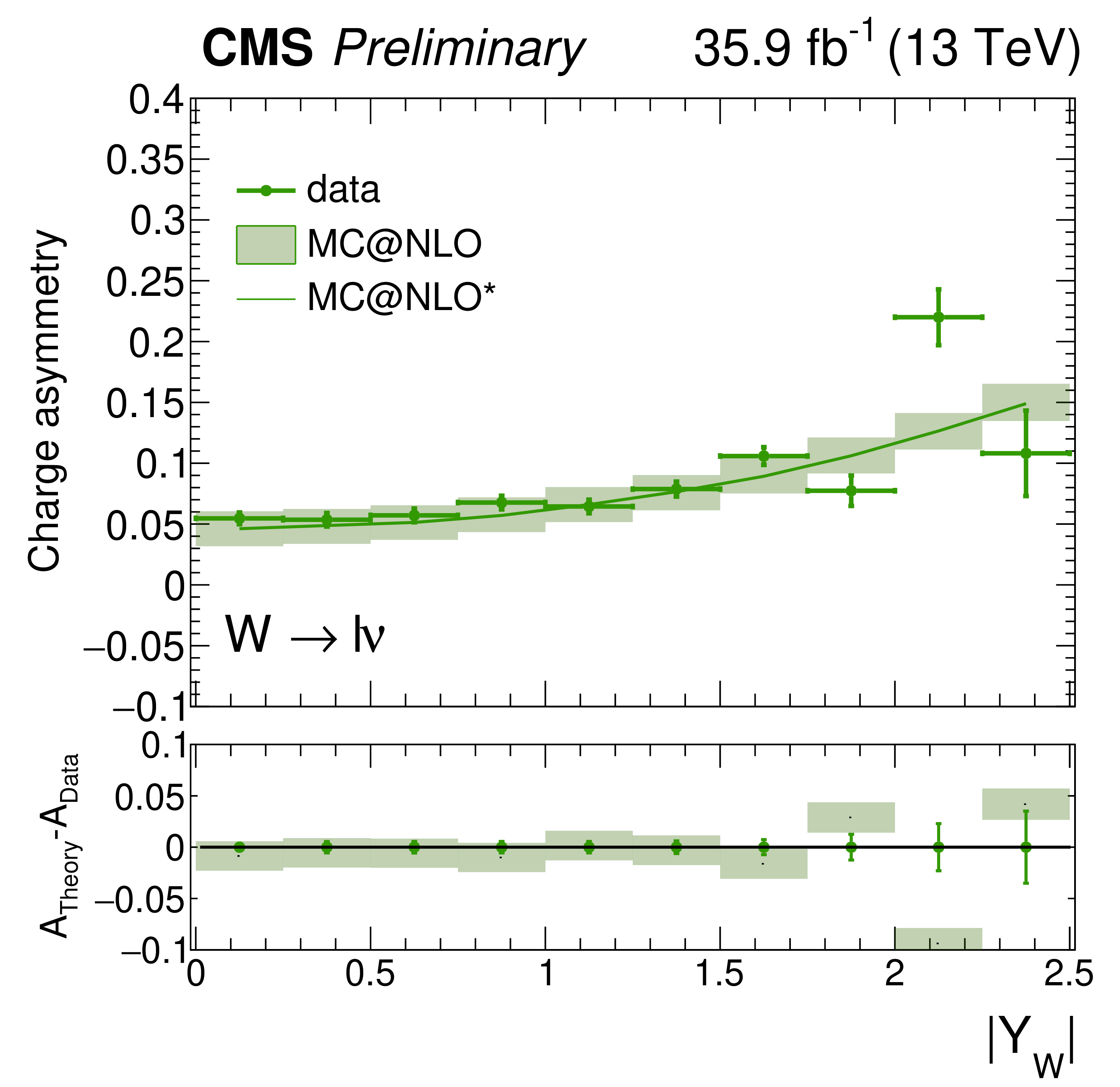
Figure 10:
Measured normalized $\mathrm{W} \to \ell ^+\nu $ (left) and $\mathrm{W} \to \ell ^-\bar\nu $ (middle) cross section as a function of $ {| Y_{\mathrm{W}} |} $ from the combination of muon and electron channels, normalized to the total cross section, integrated over the W polarization states. Right: measured W charge asymmetry. Also shown is the ratio of the prediction from MadGraph 5_aMC@NLO to the data. The light-filled band corresponds to the expected uncertainty from the PDF variations, QCD scales and $\alpha _S$. |
png pdf |
Figure 10-a:
Measured normalized $\mathrm{W} \to \ell ^+\nu $ (left) and $\mathrm{W} \to \ell ^-\bar\nu $ (middle) cross section as a function of $ {| Y_{\mathrm{W}} |} $ from the combination of muon and electron channels, normalized to the total cross section, integrated over the W polarization states. Right: measured W charge asymmetry. Also shown is the ratio of the prediction from MadGraph 5_aMC@NLO to the data. The light-filled band corresponds to the expected uncertainty from the PDF variations, QCD scales and $\alpha _S$. |
png pdf |
Figure 10-b:
Measured normalized $\mathrm{W} \to \ell ^+\nu $ (left) and $\mathrm{W} \to \ell ^-\bar\nu $ (middle) cross section as a function of $ {| Y_{\mathrm{W}} |} $ from the combination of muon and electron channels, normalized to the total cross section, integrated over the W polarization states. Right: measured W charge asymmetry. Also shown is the ratio of the prediction from MadGraph 5_aMC@NLO to the data. The light-filled band corresponds to the expected uncertainty from the PDF variations, QCD scales and $\alpha _S$. |
png pdf |
Figure 10-c:
Measured normalized $\mathrm{W} \to \ell ^+\nu $ (left) and $\mathrm{W} \to \ell ^-\bar\nu $ (middle) cross section as a function of $ {| Y_{\mathrm{W}} |} $ from the combination of muon and electron channels, normalized to the total cross section, integrated over the W polarization states. Right: measured W charge asymmetry. Also shown is the ratio of the prediction from MadGraph 5_aMC@NLO to the data. The light-filled band corresponds to the expected uncertainty from the PDF variations, QCD scales and $\alpha _S$. |
png pdf |
Figure 11:
Measured absolute $\mathrm{W} \to \ell ^+\nu $ (left) or $\mathrm{W} \to \ell ^-\bar\nu $ (right) cross section as a function of $ {| Y_{\mathrm{W}} |} $ from the combined flavor fit. Also shown is the ratio of the prediction from MadGraph 5_aMC@NLO to the data. The light-filled band corresponds to the expected uncertainty from the PDF variations, QCD scales and $\alpha _S$. |
png pdf |
Figure 11-a:
Measured absolute $\mathrm{W} \to \ell ^+\nu $ (left) or $\mathrm{W} \to \ell ^-\bar\nu $ (right) cross section as a function of $ {| Y_{\mathrm{W}} |} $ from the combined flavor fit. Also shown is the ratio of the prediction from MadGraph 5_aMC@NLO to the data. The light-filled band corresponds to the expected uncertainty from the PDF variations, QCD scales and $\alpha _S$. |

png pdf |
Figure 11-b:
Measured absolute $\mathrm{W} \to \ell ^+\nu $ (left) or $\mathrm{W} \to \ell ^-\bar\nu $ (right) cross section as a function of $ {| Y_{\mathrm{W}} |} $ from the combined flavor fit. Also shown is the ratio of the prediction from MadGraph 5_aMC@NLO to the data. The light-filled band corresponds to the expected uncertainty from the PDF variations, QCD scales and $\alpha _S$. |
png pdf |
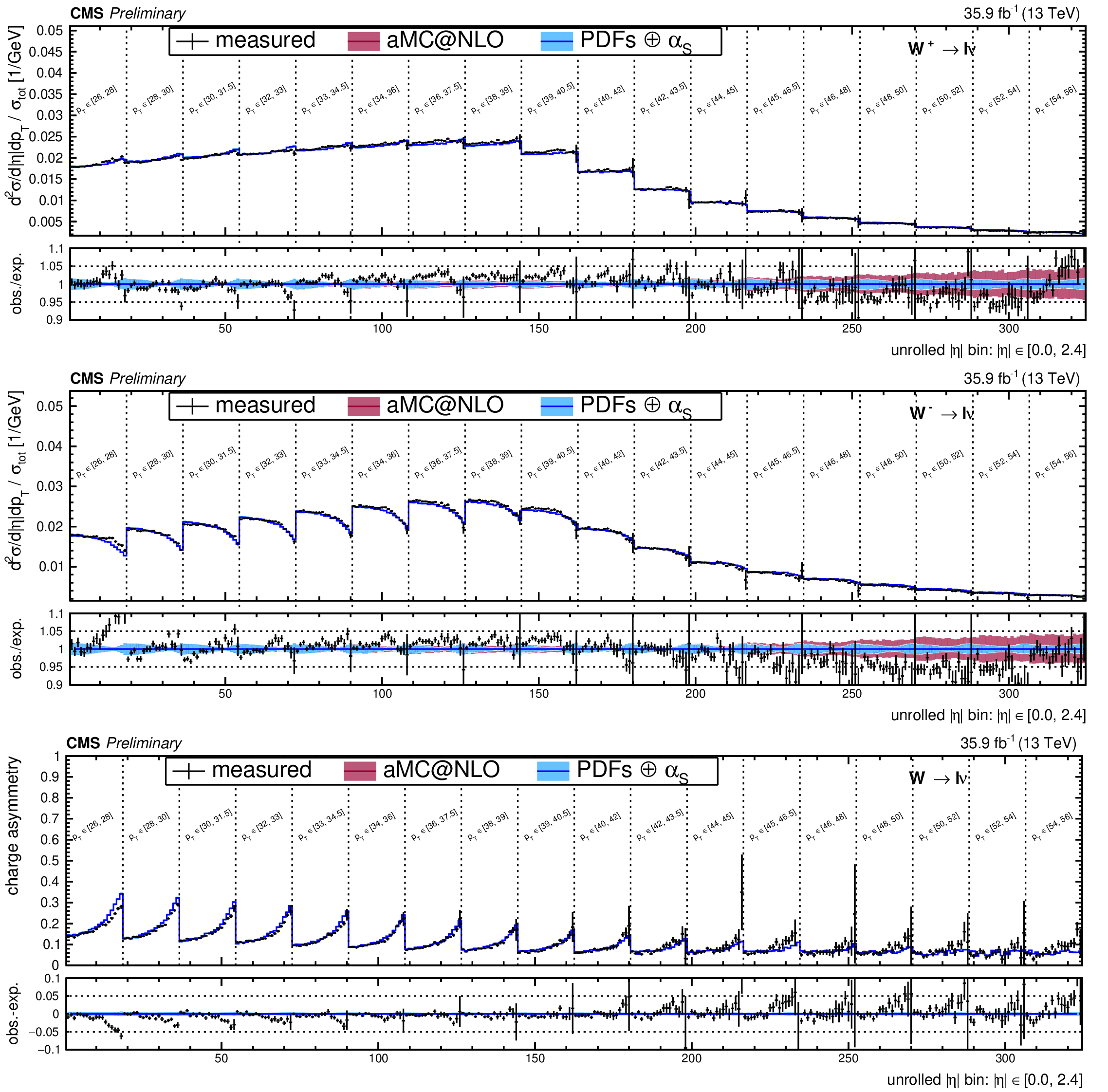
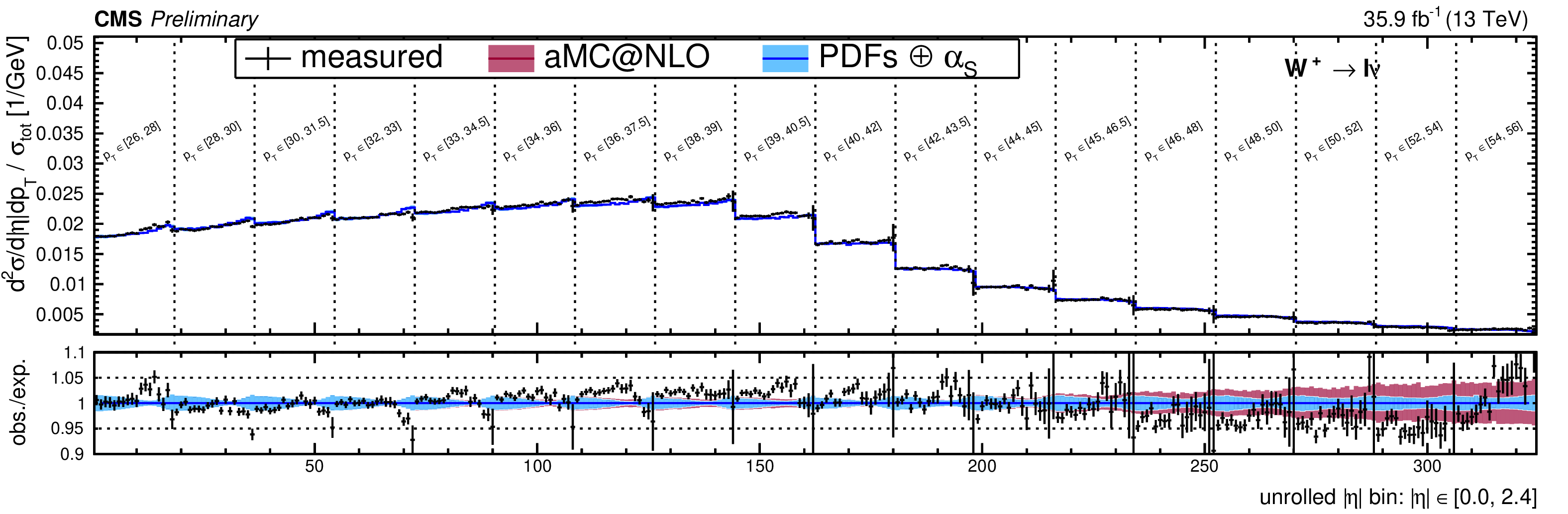
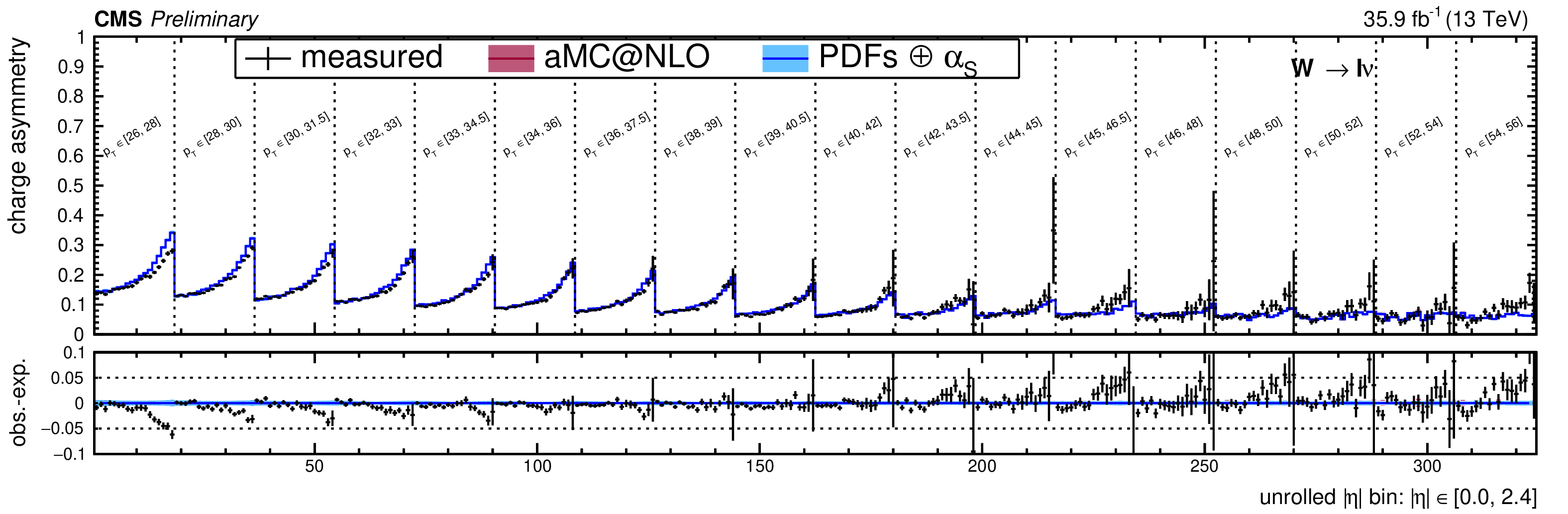
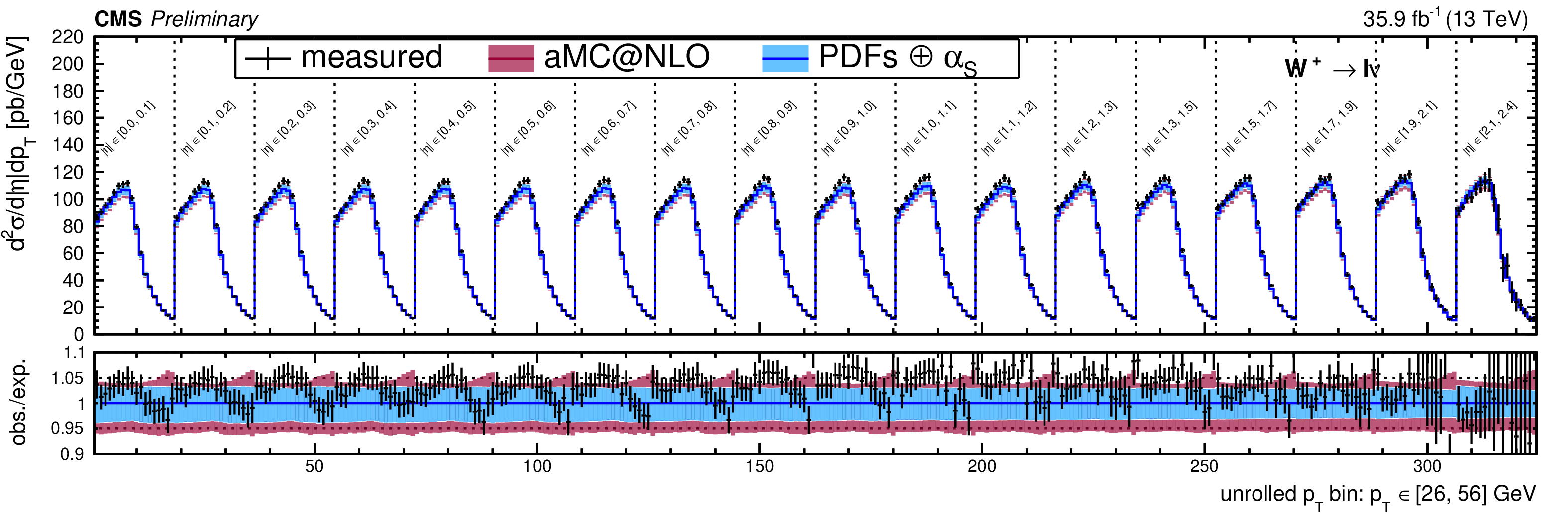
Figure 12:
Normalized double-differential cross section and charge asymmetry as a function of the ${{p_{\mathrm {T}}} ^{\ell}}$ and ${| \eta ^{\ell}|}$, unrolled in a 1D histogram along ${| \eta ^{\ell}|}$ for the positive (negative) charge on top (middle). The bottom plot shows the resulting charge asymmetry. The lower panel in each plot shows the ratio (difference) of the observed and expected cross section (asymmetry). |
png pdf |
Figure 12-a:
Normalized double-differential cross section and charge asymmetry as a function of the ${{p_{\mathrm {T}}} ^{\ell}}$ and ${| \eta ^{\ell}|}$, unrolled in a 1D histogram along ${| \eta ^{\ell}|}$ for the positive (negative) charge on top (middle). The bottom plot shows the resulting charge asymmetry. The lower panel in each plot shows the ratio (difference) of the observed and expected cross section (asymmetry). |

png pdf |
Figure 12-b:
Normalized double-differential cross section and charge asymmetry as a function of the ${{p_{\mathrm {T}}} ^{\ell}}$ and ${| \eta ^{\ell}|}$, unrolled in a 1D histogram along ${| \eta ^{\ell}|}$ for the positive (negative) charge on top (middle). The bottom plot shows the resulting charge asymmetry. The lower panel in each plot shows the ratio (difference) of the observed and expected cross section (asymmetry). |
png pdf |
Figure 12-c:
Normalized double-differential cross section and charge asymmetry as a function of the ${{p_{\mathrm {T}}} ^{\ell}}$ and ${| \eta ^{\ell}|}$, unrolled in a 1D histogram along ${| \eta ^{\ell}|}$ for the positive (negative) charge on top (middle). The bottom plot shows the resulting charge asymmetry. The lower panel in each plot shows the ratio (difference) of the observed and expected cross section (asymmetry). |
png pdf |
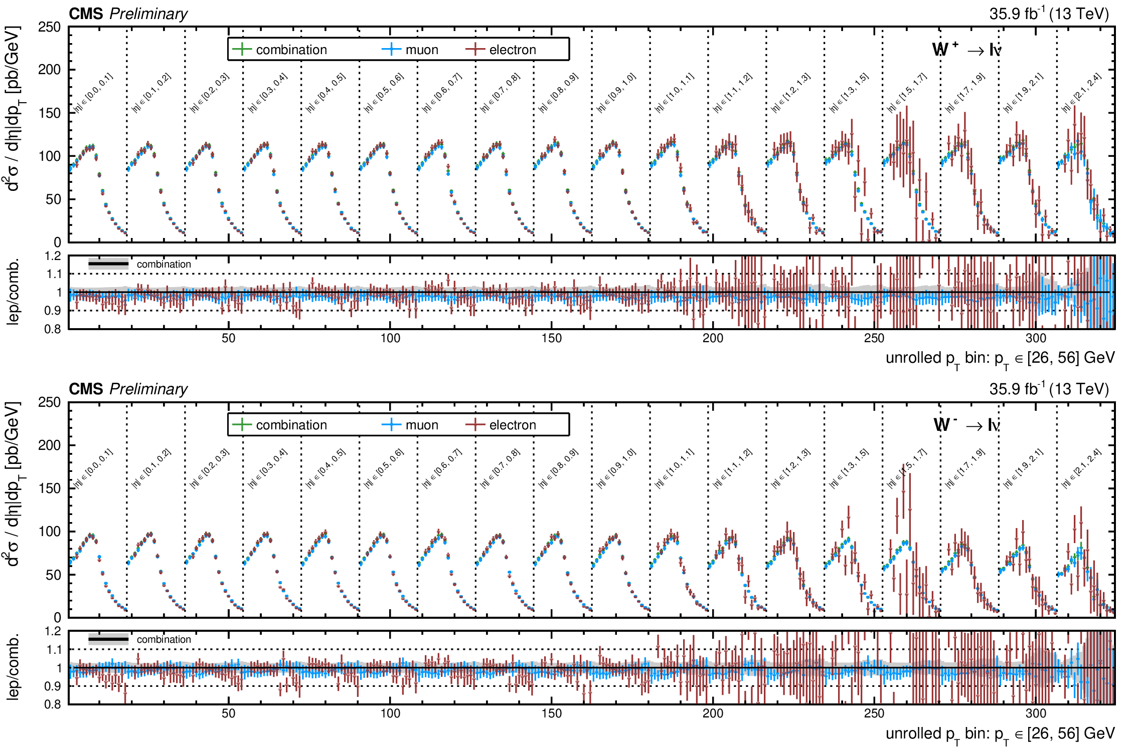
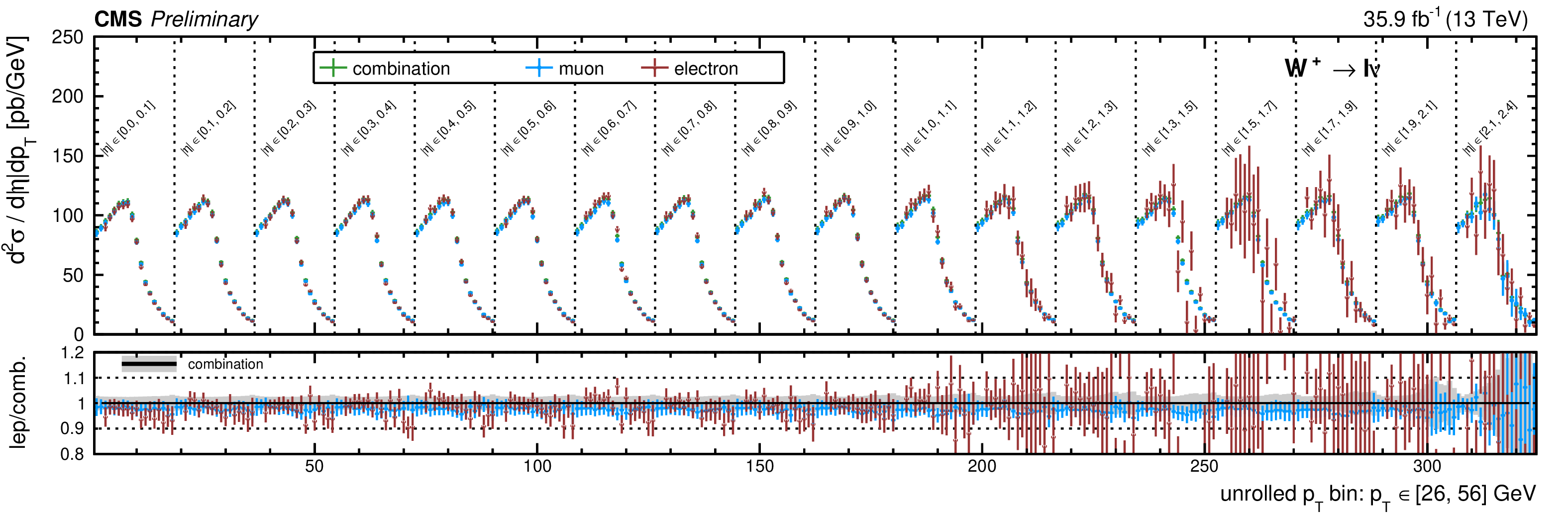
Figure 13:
Absolute double-differential cross section as a function of ${{p_{\mathrm {T}}} ^{\ell}}$ and ${| \eta ^{\ell}|}$, unrolled in a 1D histogram along ${{p_{\mathrm {T}}} ^{\ell}}$ in bins of ${| \eta ^{\ell}|}$ for the positive (negative) charge on top (bottom). The combined muon+electron fit is shown in green markers, the muon-only fit in blue markers, and the electron-only fit is shown in red markers. |
png pdf |
Figure 13-a:
Absolute double-differential cross section as a function of ${{p_{\mathrm {T}}} ^{\ell}}$ and ${| \eta ^{\ell}|}$, unrolled in a 1D histogram along ${{p_{\mathrm {T}}} ^{\ell}}$ in bins of ${| \eta ^{\ell}|}$ for the positive (negative) charge on top (bottom). The combined muon+electron fit is shown in green markers, the muon-only fit in blue markers, and the electron-only fit is shown in red markers. |

png pdf |
Figure 13-b:
Absolute double-differential cross section as a function of ${{p_{\mathrm {T}}} ^{\ell}}$ and ${| \eta ^{\ell}|}$, unrolled in a 1D histogram along ${{p_{\mathrm {T}}} ^{\ell}}$ in bins of ${| \eta ^{\ell}|}$ for the positive (negative) charge on top (bottom). The combined muon+electron fit is shown in green markers, the muon-only fit in blue markers, and the electron-only fit is shown in red markers. |
png pdf |
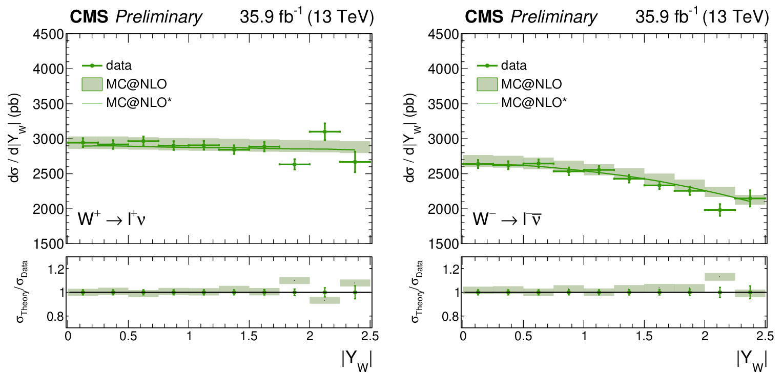
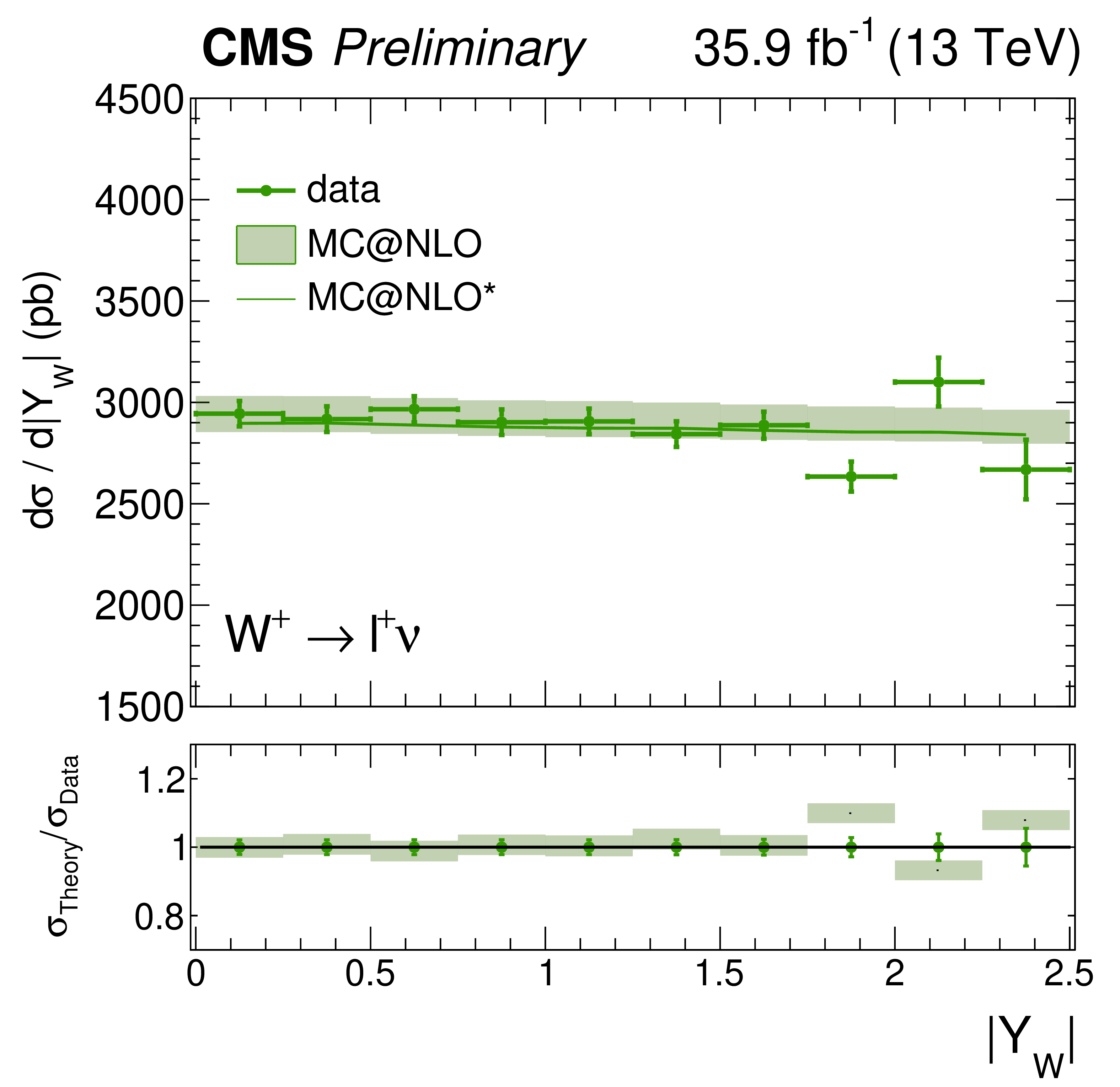
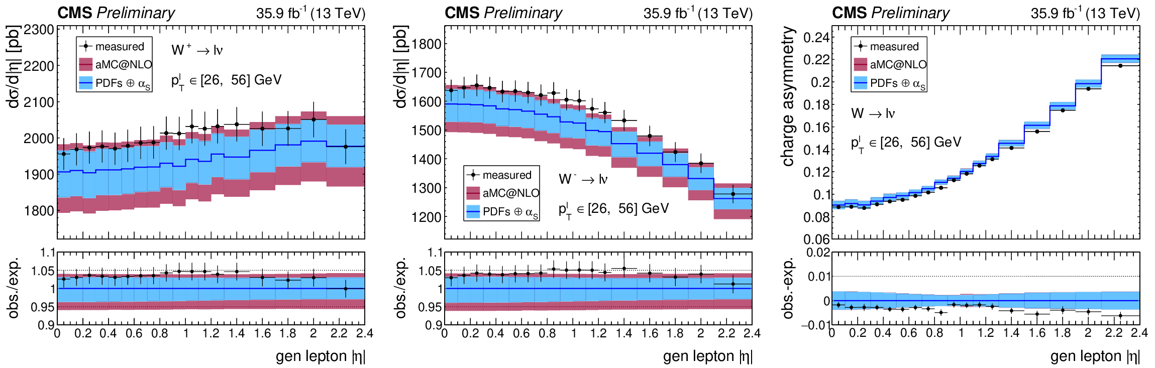
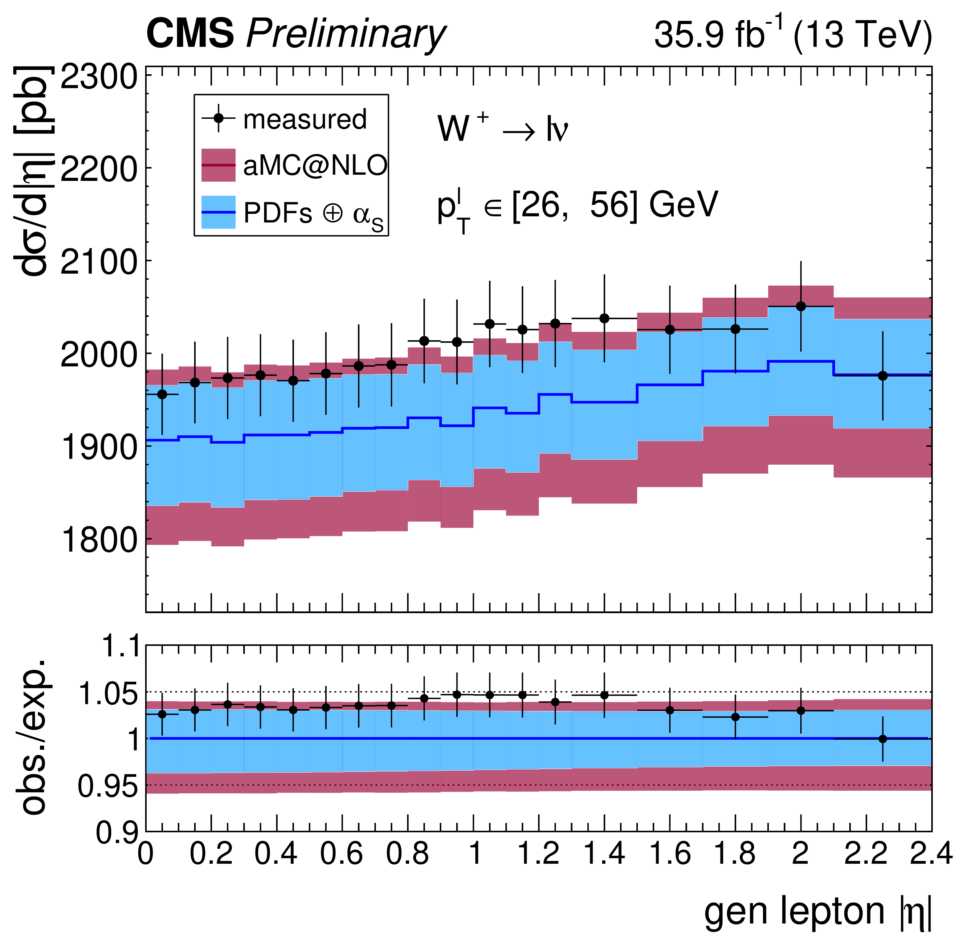
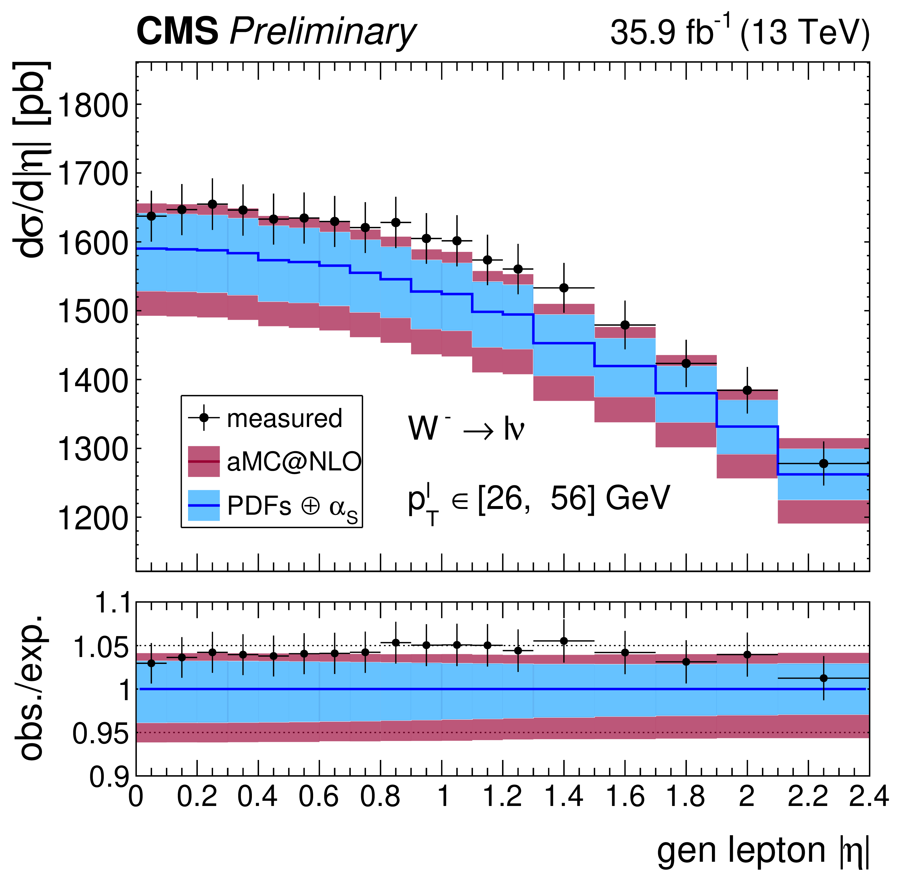
Figure 14:
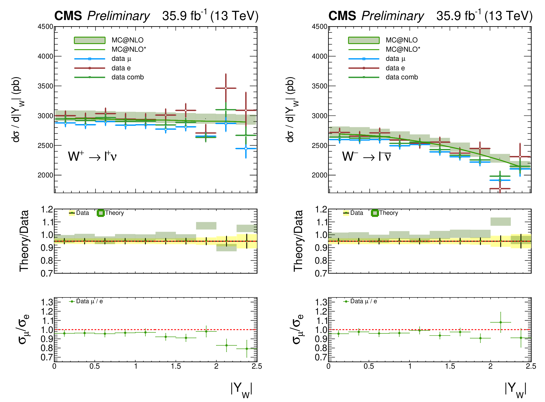
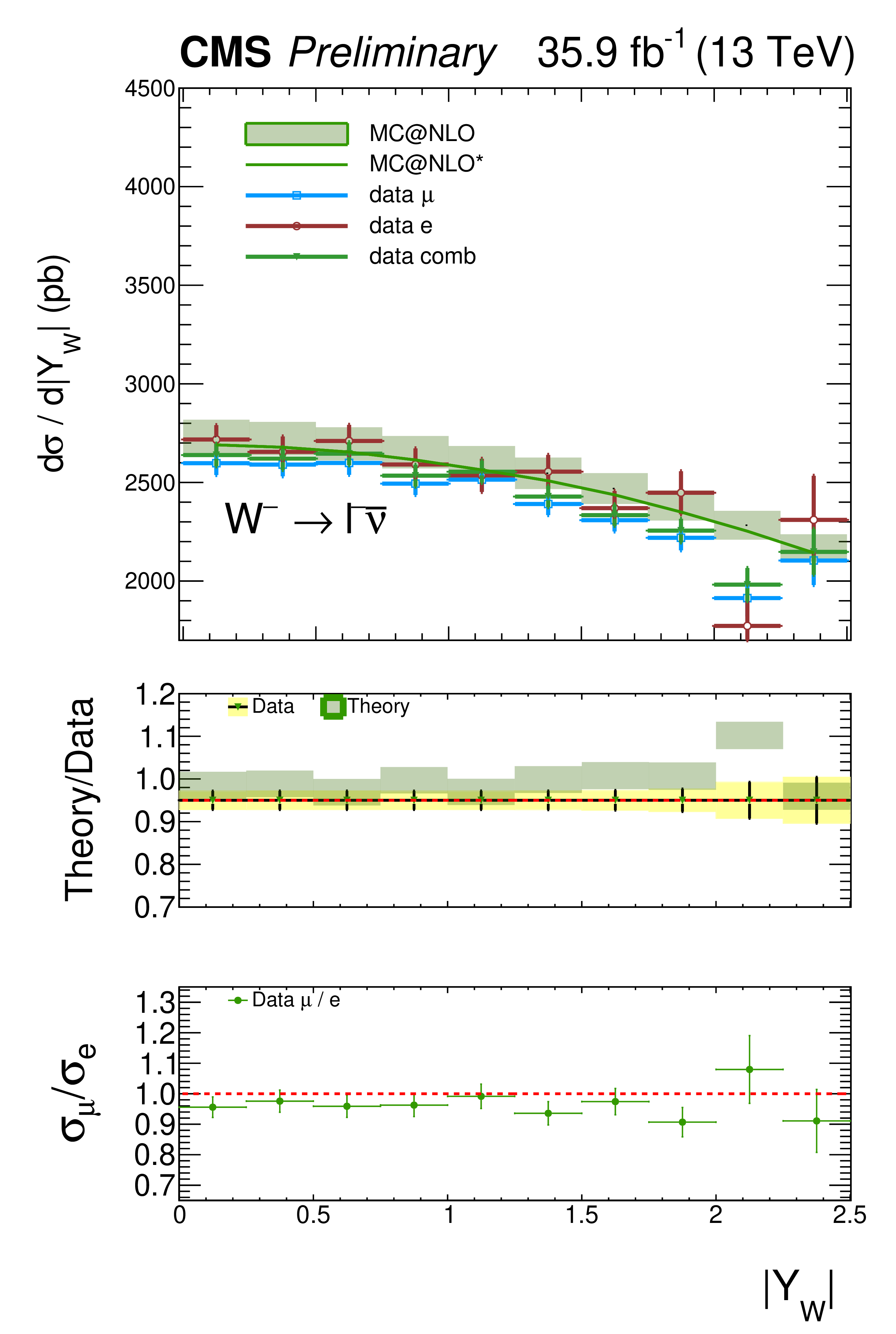
Absolute differential cross section as a function of the ${| \eta ^{\ell}|}$ for the $ {\mathrm{W} ^{+}\to \ell \nu} $ channel (left) and $ {\mathrm{W} ^{-}\to \ell \bar\nu} $ channel (middle). The corresponding charge asymmetry is shown on the right. The measurement is the result of the combination of the electron and muon channels. The lower panel in each plot shows the ratio (difference) of observation and expectation for the cross section (asymmetry) and the relative uncertainty. |
png pdf |
Figure 14-a:
Absolute differential cross section as a function of the ${| \eta ^{\ell}|}$ for the $ {\mathrm{W} ^{+}\to \ell \nu} $ channel (left) and $ {\mathrm{W} ^{-}\to \ell \bar\nu} $ channel (middle). The corresponding charge asymmetry is shown on the right. The measurement is the result of the combination of the electron and muon channels. The lower panel in each plot shows the ratio (difference) of observation and expectation for the cross section (asymmetry) and the relative uncertainty. |
png pdf |
Figure 14-b:
Absolute differential cross section as a function of the ${| \eta ^{\ell}|}$ for the $ {\mathrm{W} ^{+}\to \ell \nu} $ channel (left) and $ {\mathrm{W} ^{-}\to \ell \bar\nu} $ channel (middle). The corresponding charge asymmetry is shown on the right. The measurement is the result of the combination of the electron and muon channels. The lower panel in each plot shows the ratio (difference) of observation and expectation for the cross section (asymmetry) and the relative uncertainty. |

png pdf |
Figure 14-c:
Absolute differential cross section as a function of the ${| \eta ^{\ell}|}$ for the $ {\mathrm{W} ^{+}\to \ell \nu} $ channel (left) and $ {\mathrm{W} ^{-}\to \ell \bar\nu} $ channel (middle). The corresponding charge asymmetry is shown on the right. The measurement is the result of the combination of the electron and muon channels. The lower panel in each plot shows the ratio (difference) of observation and expectation for the cross section (asymmetry) and the relative uncertainty. |
png pdf |
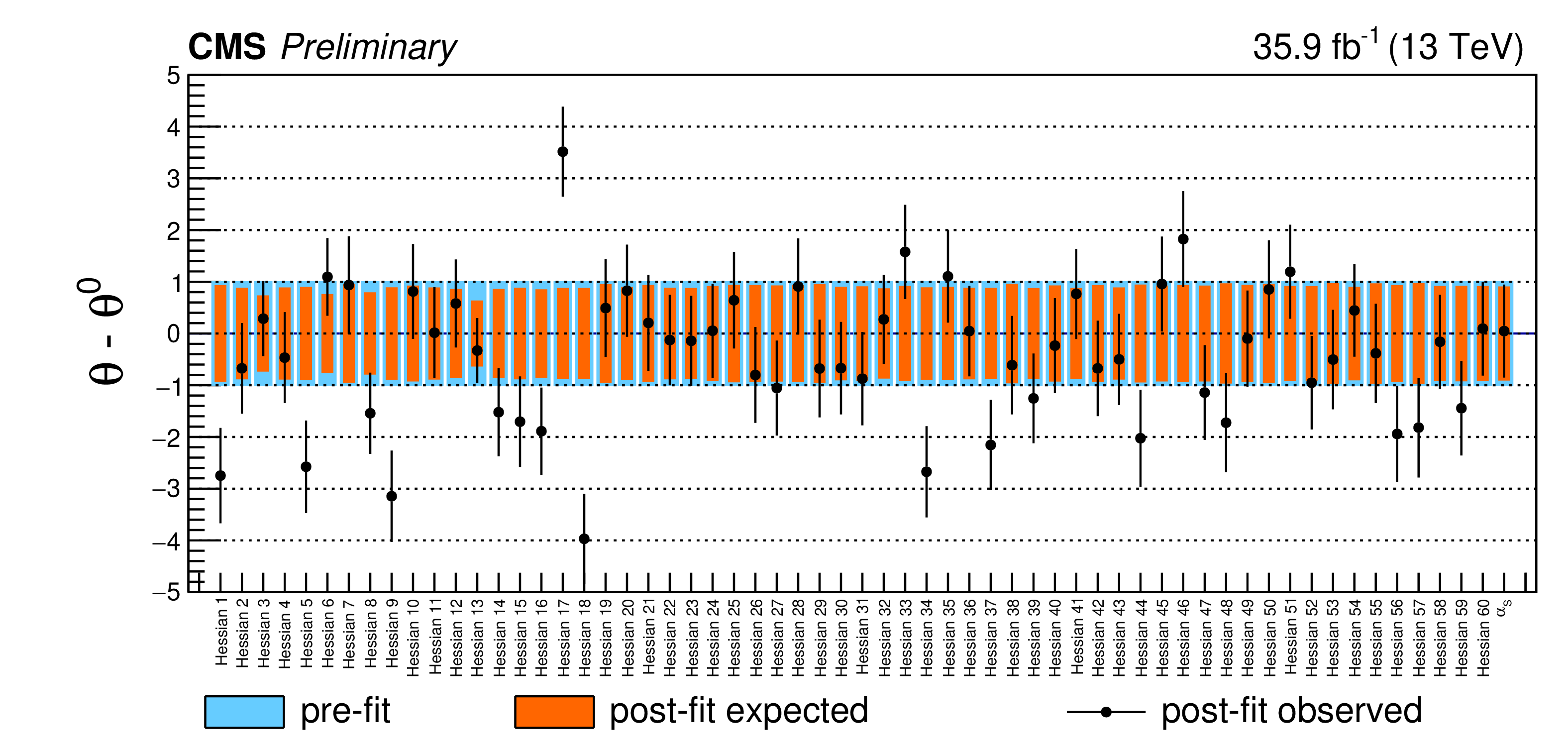
Figure 15:
Pulls and constraints of the 60 Hessian variations of the NNPDF3.0 PDF set, and of the $\alpha _S$ parameter, from the combined fit of muon and electron channels. The underlying fit is performed by fixing the W cross sections to their expectation in all helicity and charge processes. The cyan band represents the input values (which all have zero mean and width one), the orange bands show the post-fit expected values, and black points represent the observed pulls and constraint values. The post-fit nuisance parameter values with respect to the prefit values and uncertainties give a $\chi ^2/dof$ of $117/61$. |

png pdf |
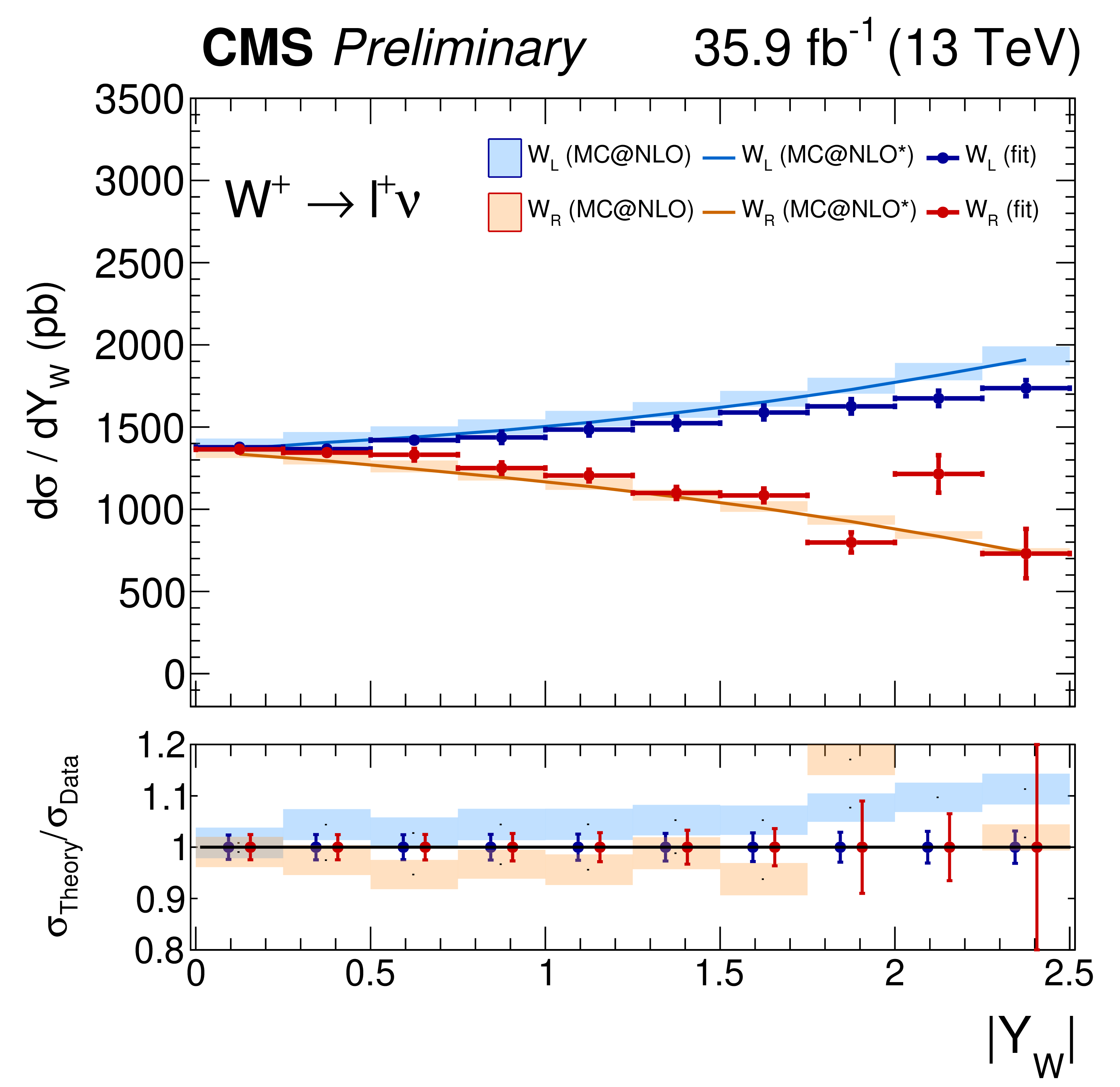
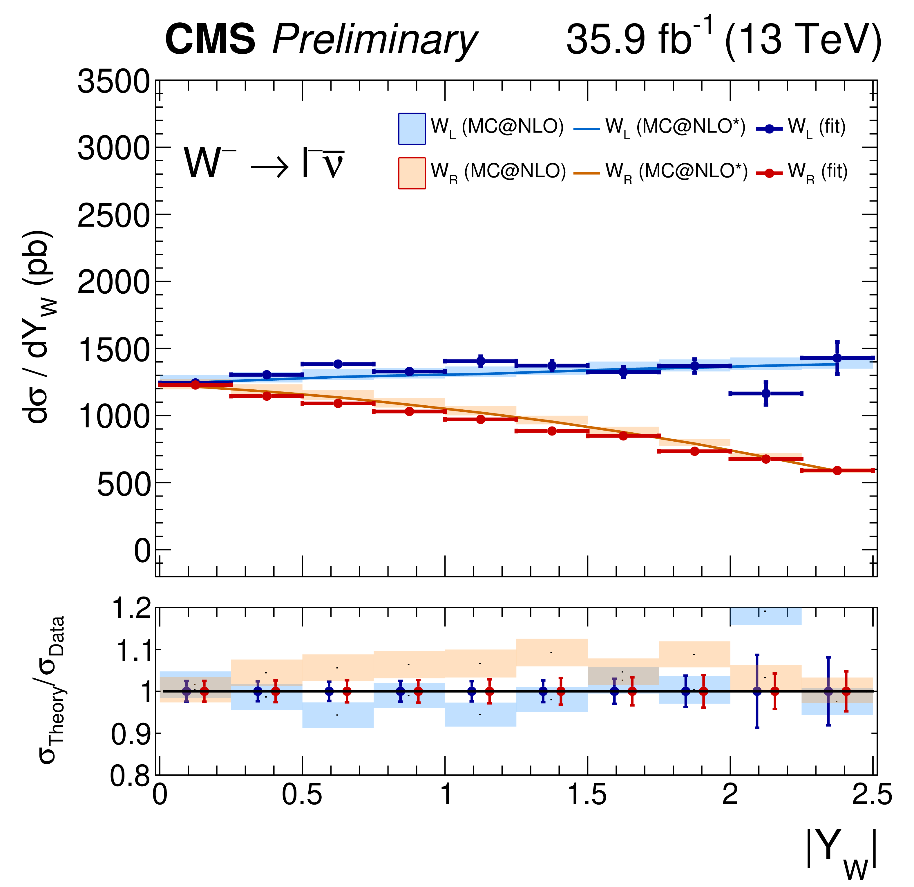
Figure 16:
Measured absolute $\mathrm{W} \to \ell ^+\nu $ (left) and $\mathrm{W} \to \ell ^-\bar\nu $ (right) cross section as a function of $ {| Y_{\mathrm{W}} |} $ for the left-handed and right-handed helicity states from the combination of muon and electron channels. Also shown is the ratio of the prediction from MadGraph 5_aMC@NLO to the data. The light-filled band corresponds to the expected uncertainty from the PDF variations, QCD scales and $\alpha _S$. |
png pdf |
Figure 16-a:
Measured absolute $\mathrm{W} \to \ell ^+\nu $ (left) and $\mathrm{W} \to \ell ^-\bar\nu $ (right) cross section as a function of $ {| Y_{\mathrm{W}} |} $ for the left-handed and right-handed helicity states from the combination of muon and electron channels. Also shown is the ratio of the prediction from MadGraph 5_aMC@NLO to the data. The light-filled band corresponds to the expected uncertainty from the PDF variations, QCD scales and $\alpha _S$. |
png pdf |
Figure 16-b:
Measured absolute $\mathrm{W} \to \ell ^+\nu $ (left) and $\mathrm{W} \to \ell ^-\bar\nu $ (right) cross section as a function of $ {| Y_{\mathrm{W}} |} $ for the left-handed and right-handed helicity states from the combination of muon and electron channels. Also shown is the ratio of the prediction from MadGraph 5_aMC@NLO to the data. The light-filled band corresponds to the expected uncertainty from the PDF variations, QCD scales and $\alpha _S$. |
png pdf |
Figure 17:
Measured absolute $\mathrm{W} \to \ell ^+\nu $ (left) or $\mathrm{W} \to \ell ^-\bar\nu $ (right) cross section as a function of $ {| Y_{\mathrm{W}} |} $ from three distinct fits: the combination of muon and electron channels (green), the muon-only fit (blue), and the electron-only fit (red) in the top panel. Also shown is the ratio of the prediction from MadGraph 5_aMC@NLO to the data in the middle panel, as well as the ratio between the muon-only fit and the electron-only fit in the bottom panel. The light-filled band corresponds to the expected uncertainty from the PDF variations, QCD scales and $\alpha _S$. |

png pdf |
Figure 17-a:
Measured absolute $\mathrm{W} \to \ell ^+\nu $ (left) or $\mathrm{W} \to \ell ^-\bar\nu $ (right) cross section as a function of $ {| Y_{\mathrm{W}} |} $ from three distinct fits: the combination of muon and electron channels (green), the muon-only fit (blue), and the electron-only fit (red) in the top panel. Also shown is the ratio of the prediction from MadGraph 5_aMC@NLO to the data in the middle panel, as well as the ratio between the muon-only fit and the electron-only fit in the bottom panel. The light-filled band corresponds to the expected uncertainty from the PDF variations, QCD scales and $\alpha _S$. |
png pdf |
Figure 17-b:
Measured absolute $\mathrm{W} \to \ell ^+\nu $ (left) or $\mathrm{W} \to \ell ^-\bar\nu $ (right) cross section as a function of $ {| Y_{\mathrm{W}} |} $ from three distinct fits: the combination of muon and electron channels (green), the muon-only fit (blue), and the electron-only fit (red) in the top panel. Also shown is the ratio of the prediction from MadGraph 5_aMC@NLO to the data in the middle panel, as well as the ratio between the muon-only fit and the electron-only fit in the bottom panel. The light-filled band corresponds to the expected uncertainty from the PDF variations, QCD scales and $\alpha _S$. |
png pdf |
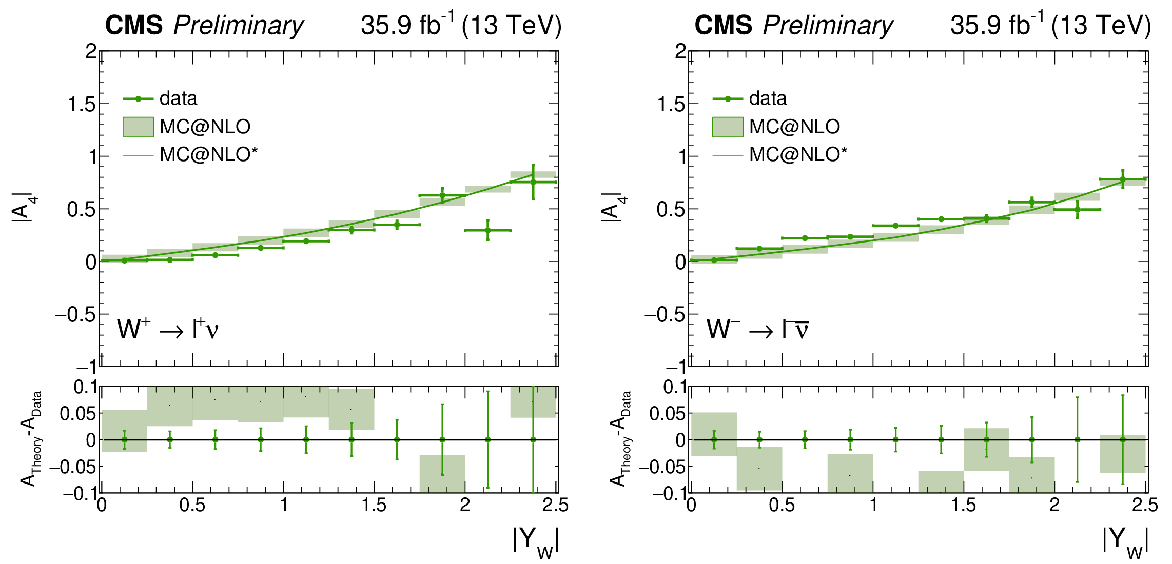
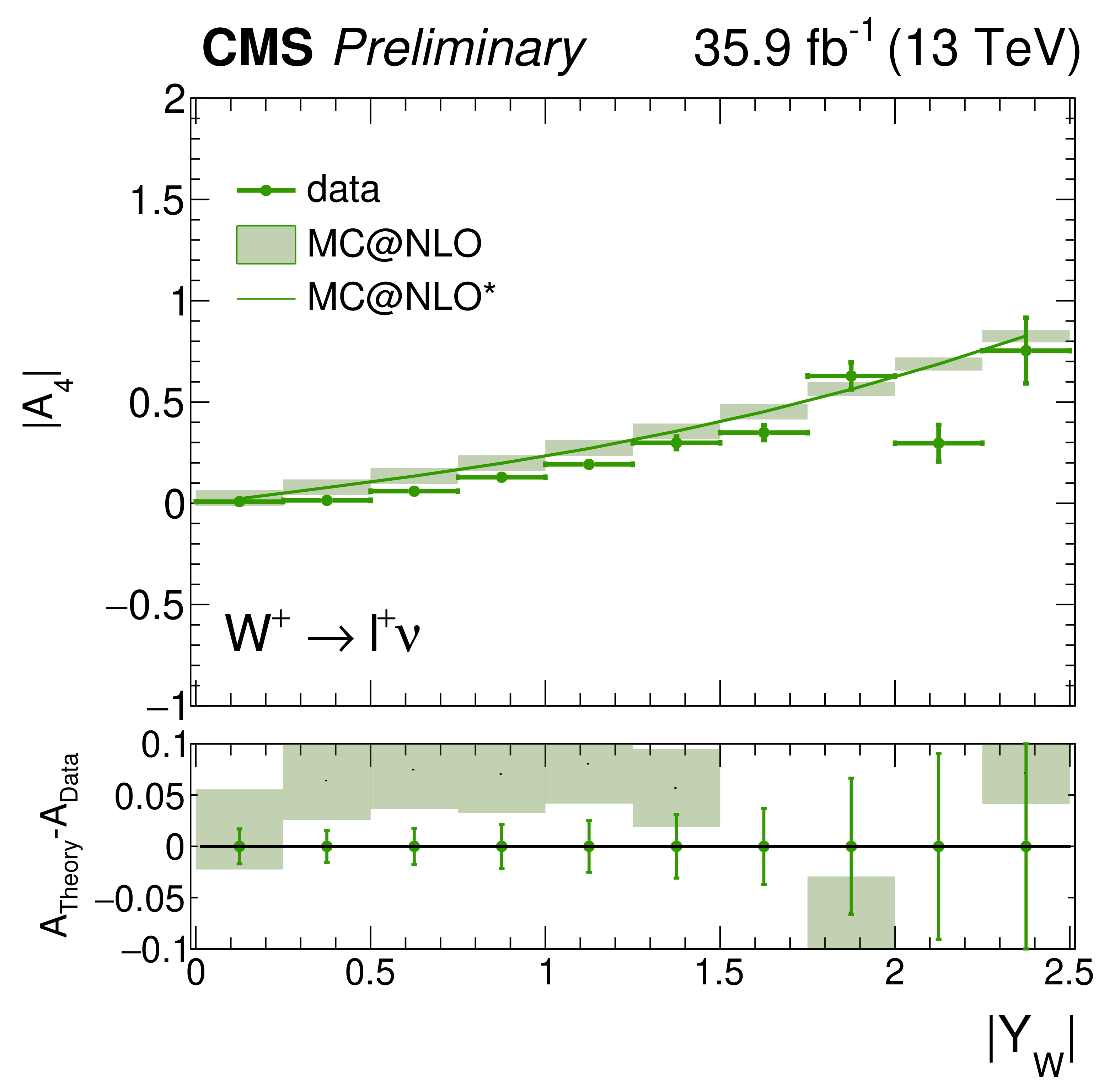
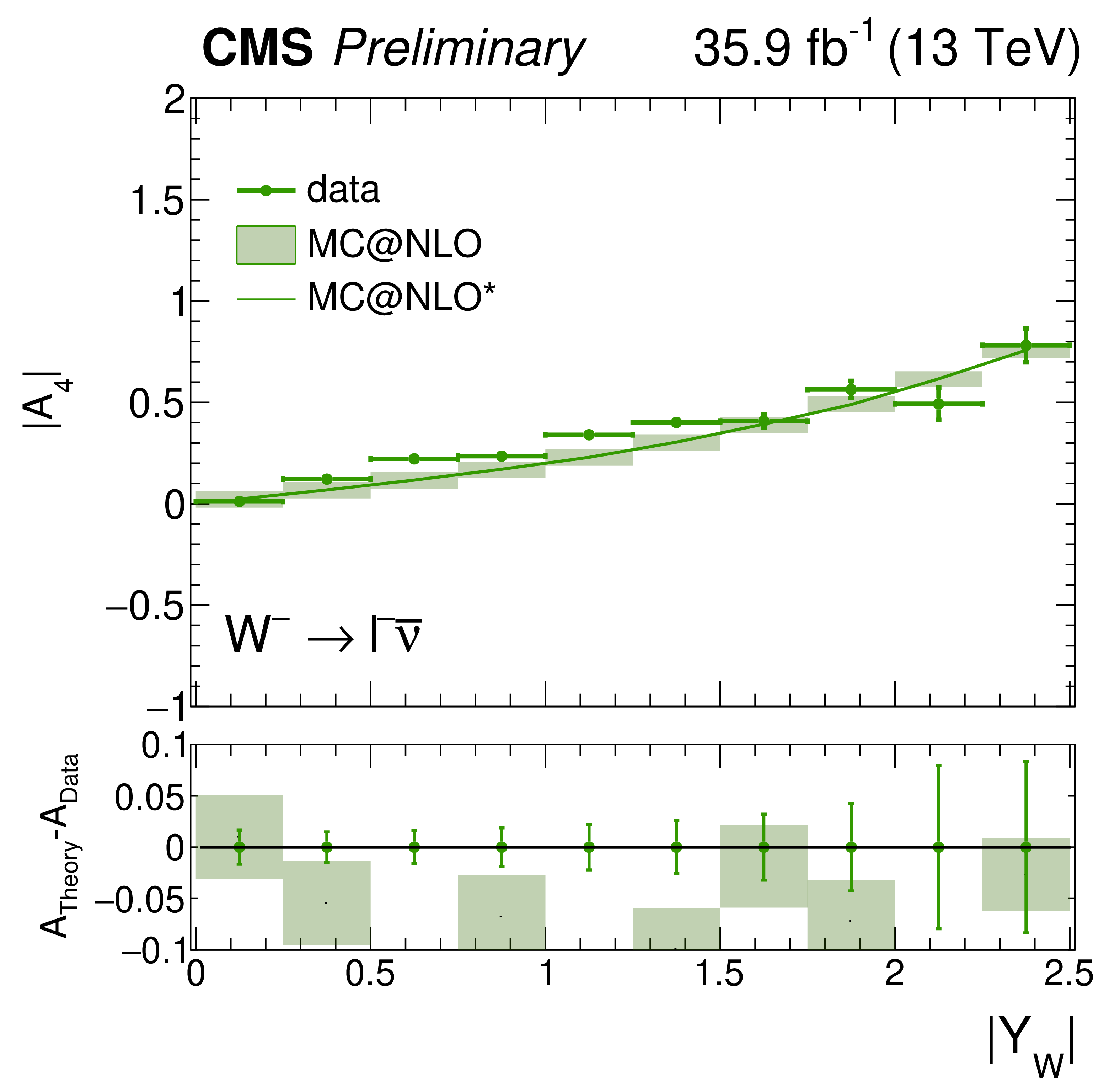
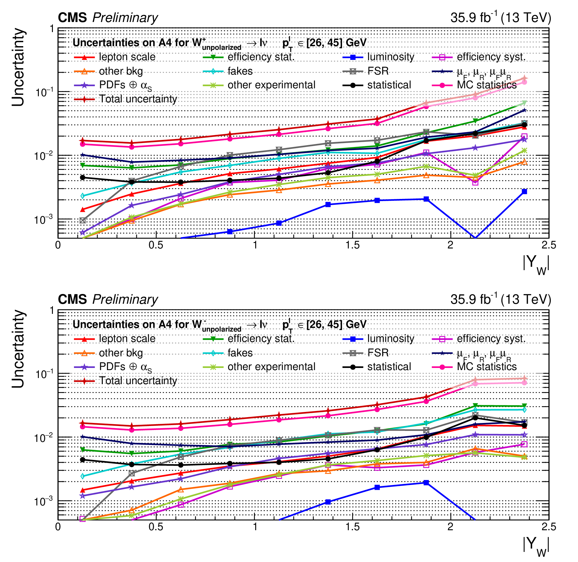
Figure 18:
Measured $A_4$ coefficient for $\mathrm{W} \to \ell ^+\nu $ (left) and $\mathrm{W} \to \ell ^-\bar\nu $ (right) extracted from the fit of the polarized cross sections to the combined electron+muon fit. Also shown is the difference between the prediction from MadGraph 5_aMC@NLO and the measured values. The light-filled band corresponds to the expected uncertainty from the PDF variations, QCD scales and $\alpha _S$. |
png pdf |
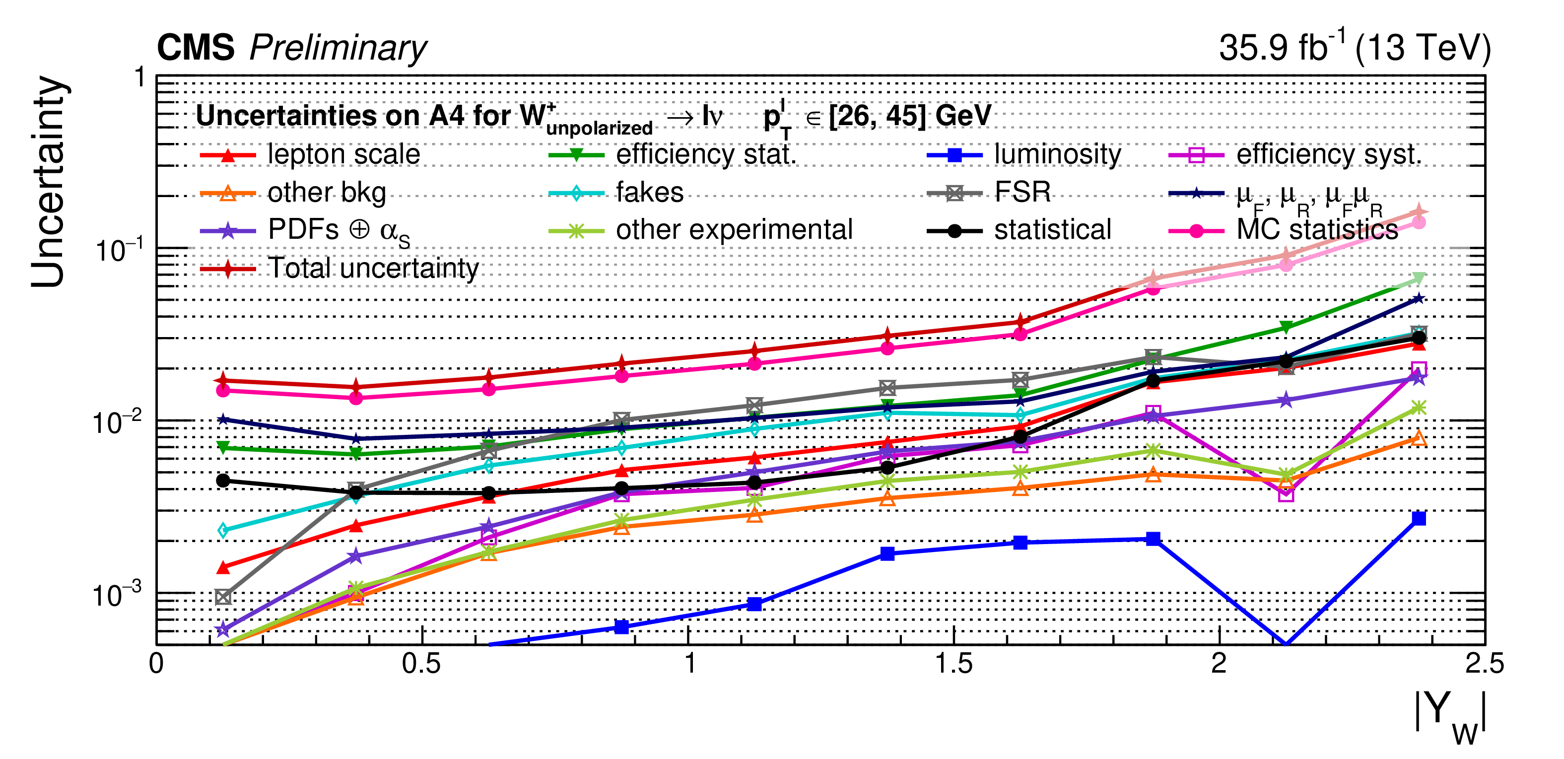
Figure 18-a:
Measured $A_4$ coefficient for $\mathrm{W} \to \ell ^+\nu $ (left) and $\mathrm{W} \to \ell ^-\bar\nu $ (right) extracted from the fit of the polarized cross sections to the combined electron+muon fit. Also shown is the difference between the prediction from MadGraph 5_aMC@NLO and the measured values. The light-filled band corresponds to the expected uncertainty from the PDF variations, QCD scales and $\alpha _S$. |
png pdf |
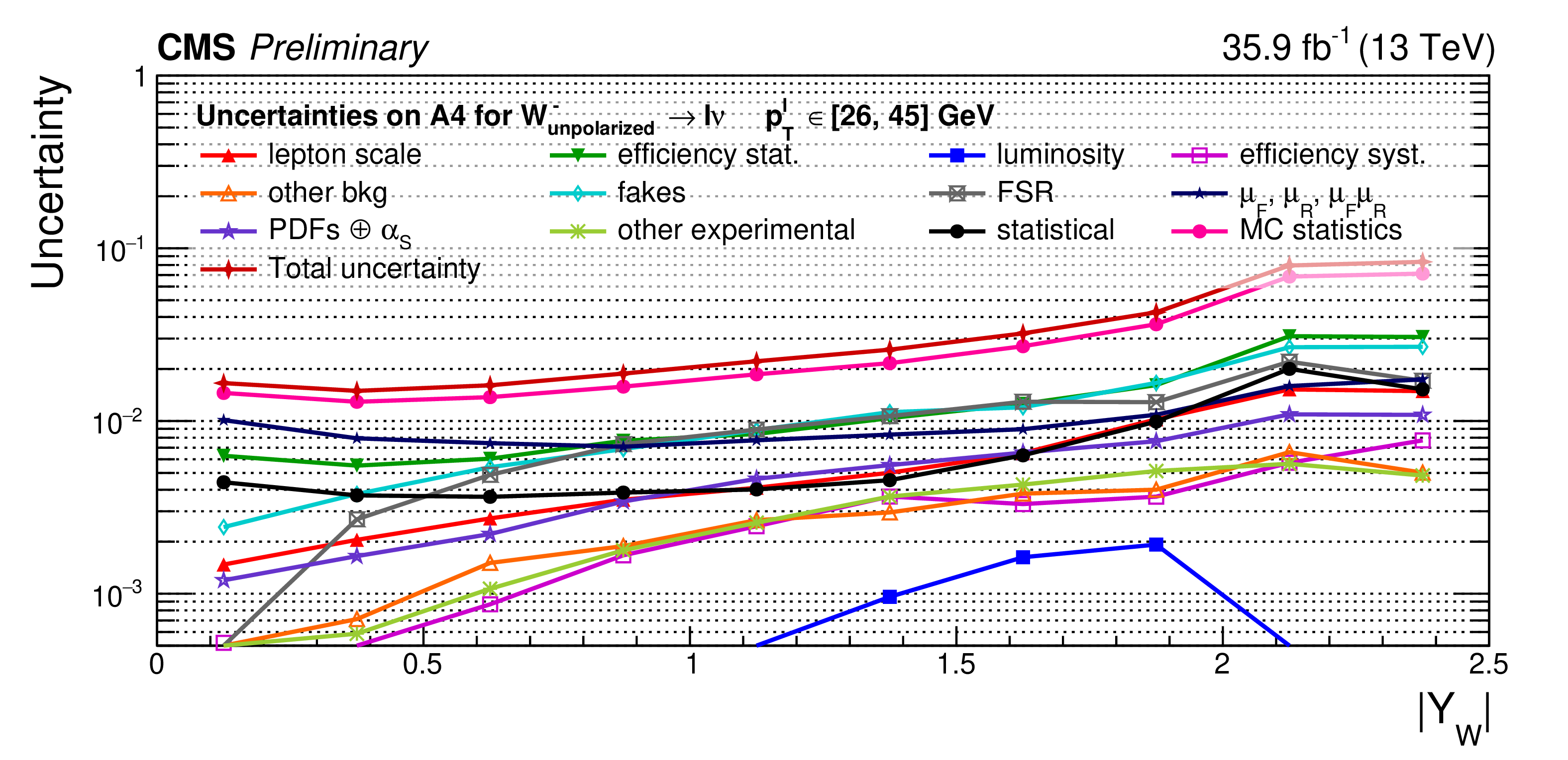
Figure 18-b:
Measured $A_4$ coefficient for $\mathrm{W} \to \ell ^+\nu $ (left) and $\mathrm{W} \to \ell ^-\bar\nu $ (right) extracted from the fit of the polarized cross sections to the combined electron+muon fit. Also shown is the difference between the prediction from MadGraph 5_aMC@NLO and the measured values. The light-filled band corresponds to the expected uncertainty from the PDF variations, QCD scales and $\alpha _S$. |
png pdf |
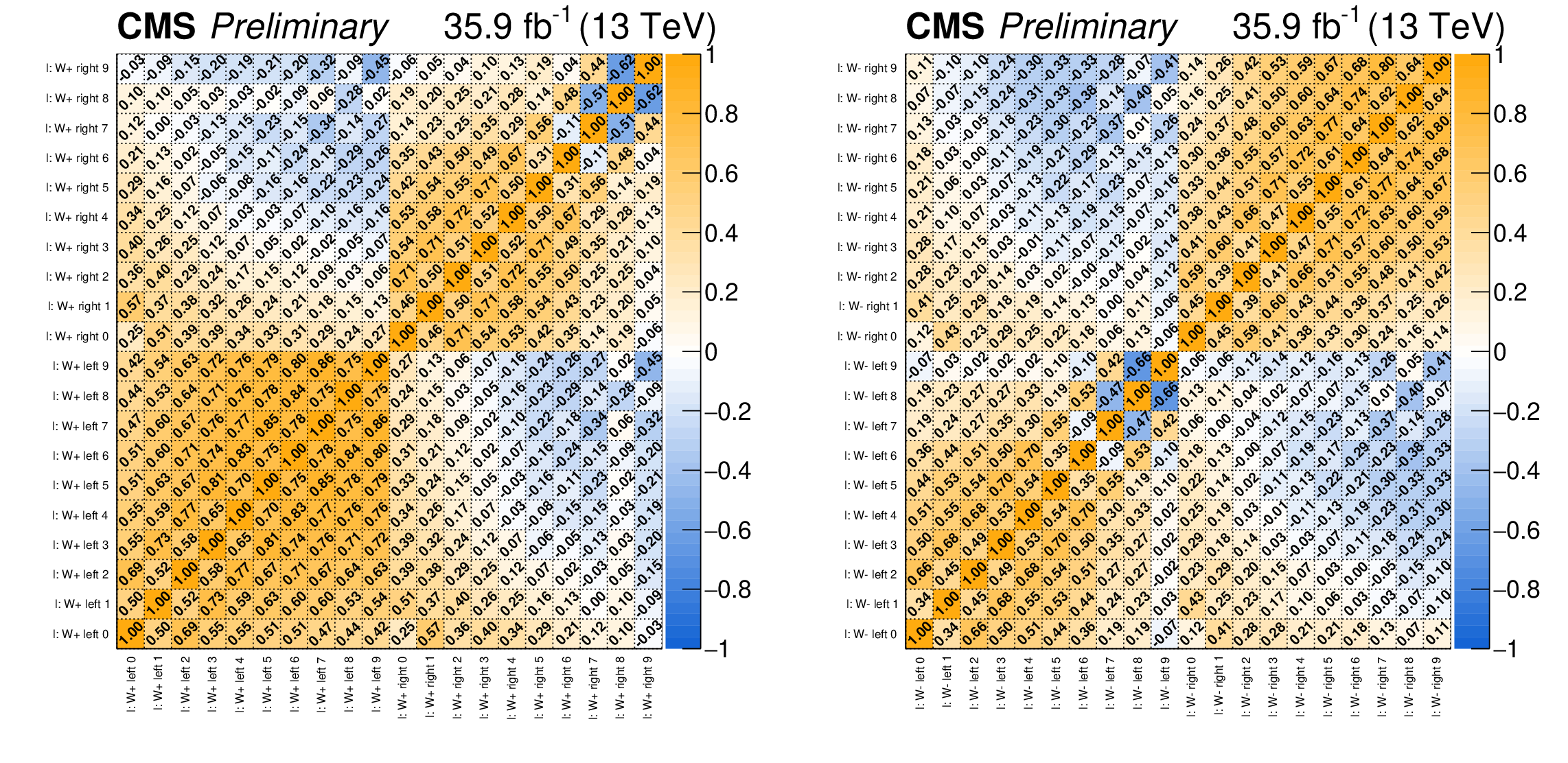
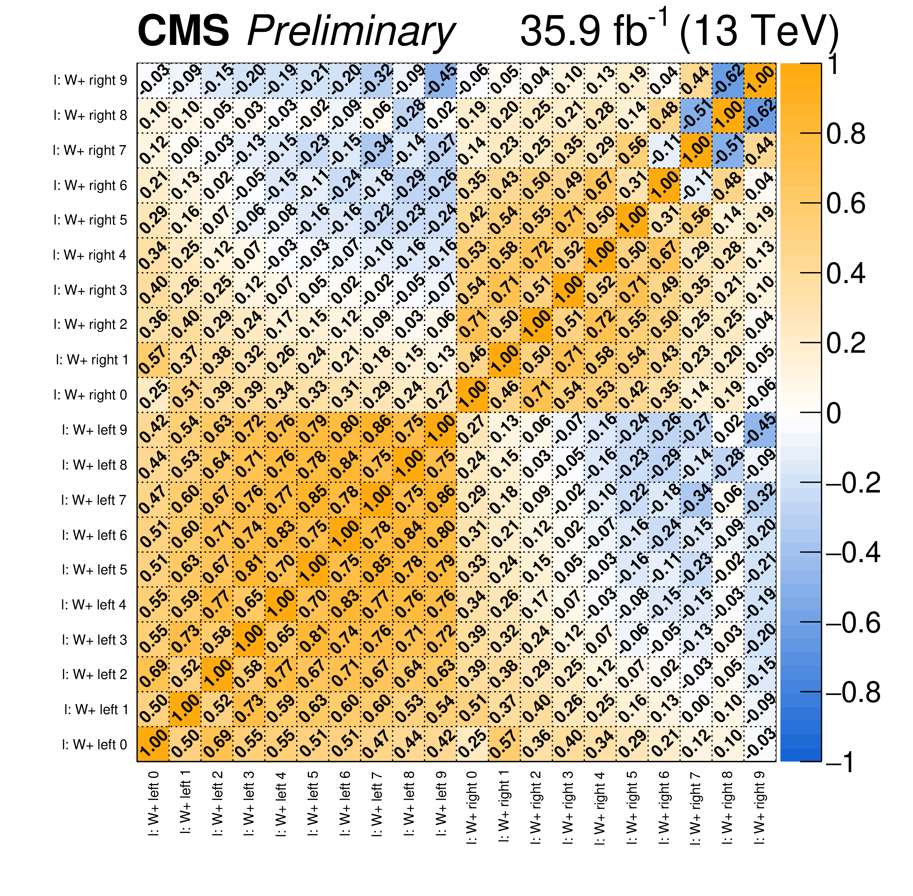
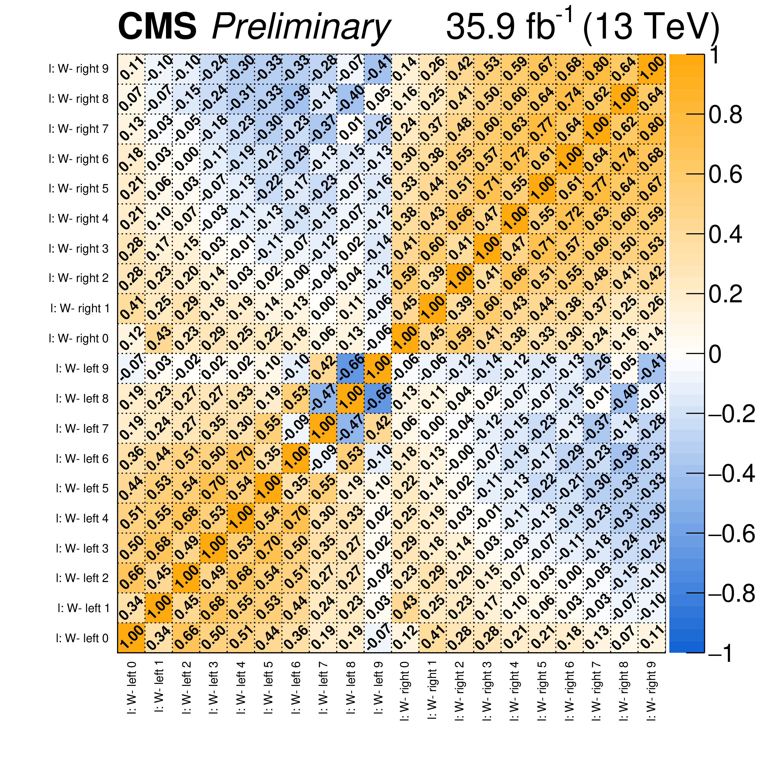
Figure 19:
Correlation coefficients between the helicity-dependent signal cross sections for $\mathrm{W} \to \ell ^+\nu $ (left) and $\mathrm{W} \to \ell ^-\bar\nu $ (right) extracted from the fit to the combined electron+muon fit. |
png pdf |
Figure 19-a:
Correlation coefficients between the helicity-dependent signal cross sections for $\mathrm{W} \to \ell ^+\nu $ (left) and $\mathrm{W} \to \ell ^-\bar\nu $ (right) extracted from the fit to the combined electron+muon fit. |
png pdf |
Figure 19-b:
Correlation coefficients between the helicity-dependent signal cross sections for $\mathrm{W} \to \ell ^+\nu $ (left) and $\mathrm{W} \to \ell ^-\bar\nu $ (right) extracted from the fit to the combined electron+muon fit. |
png pdf |
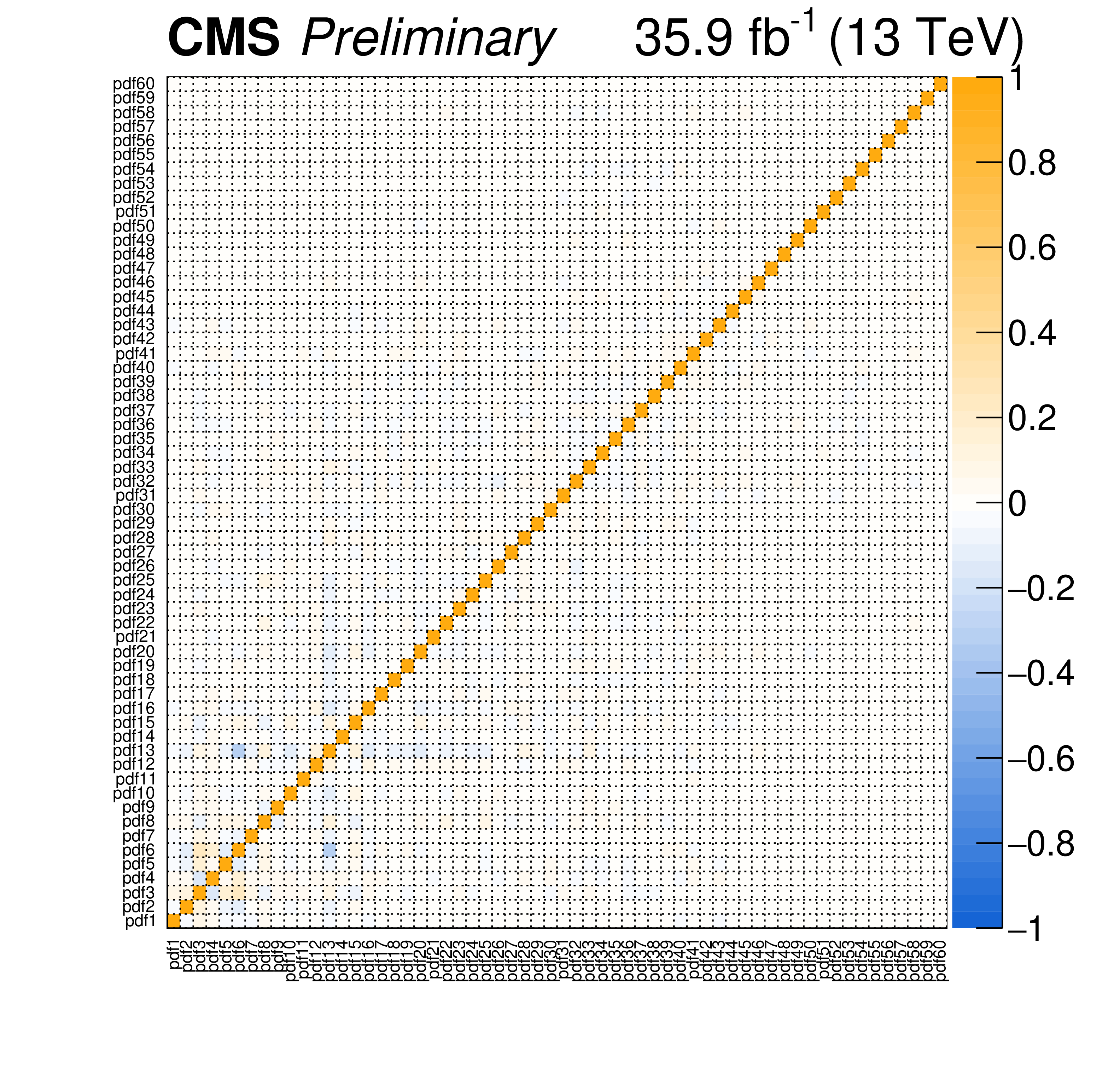
Figure 20:
Correlation coefficients between the 60 PDF nuisance parameters extracted from the fit to the combined electron+muon fit. |

png pdf |
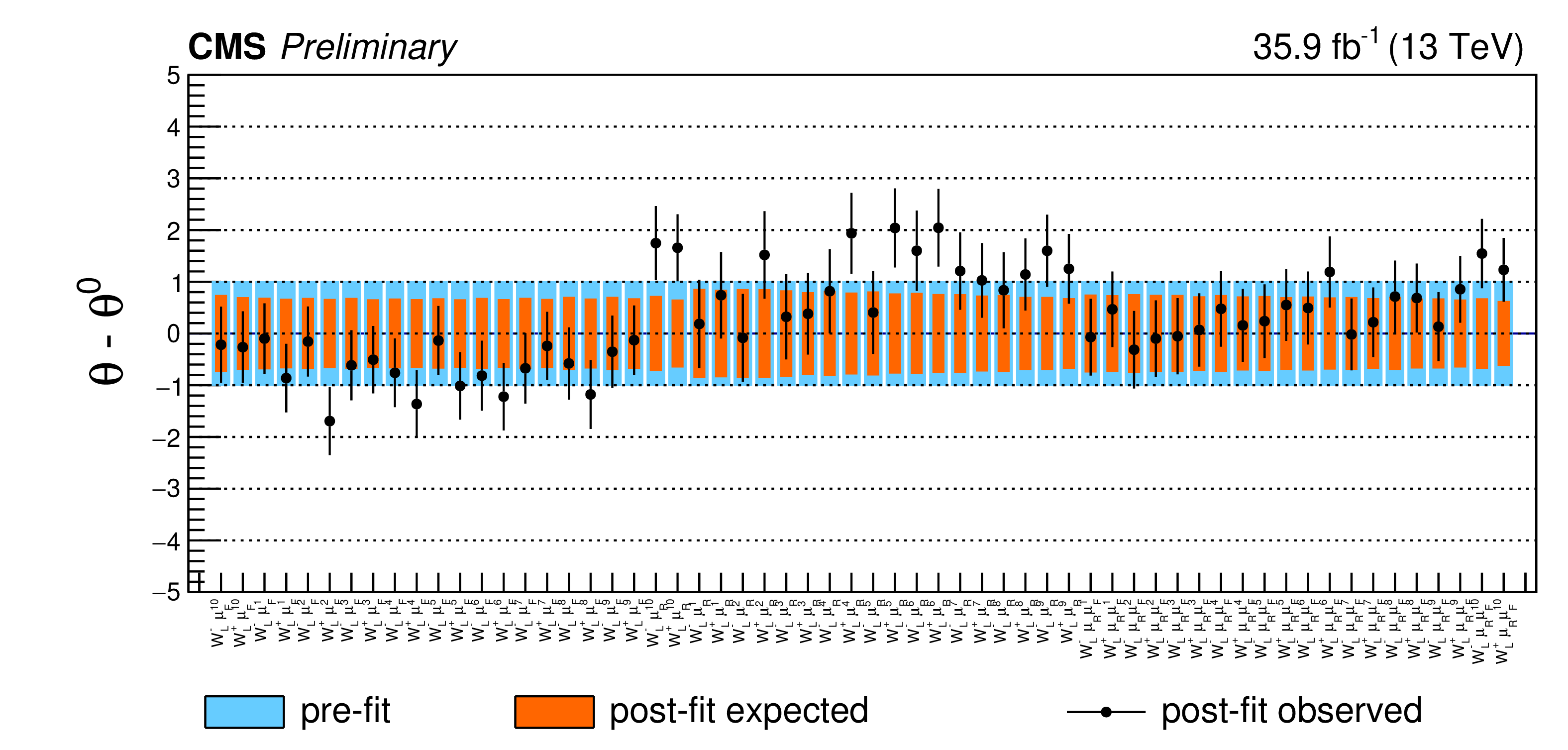
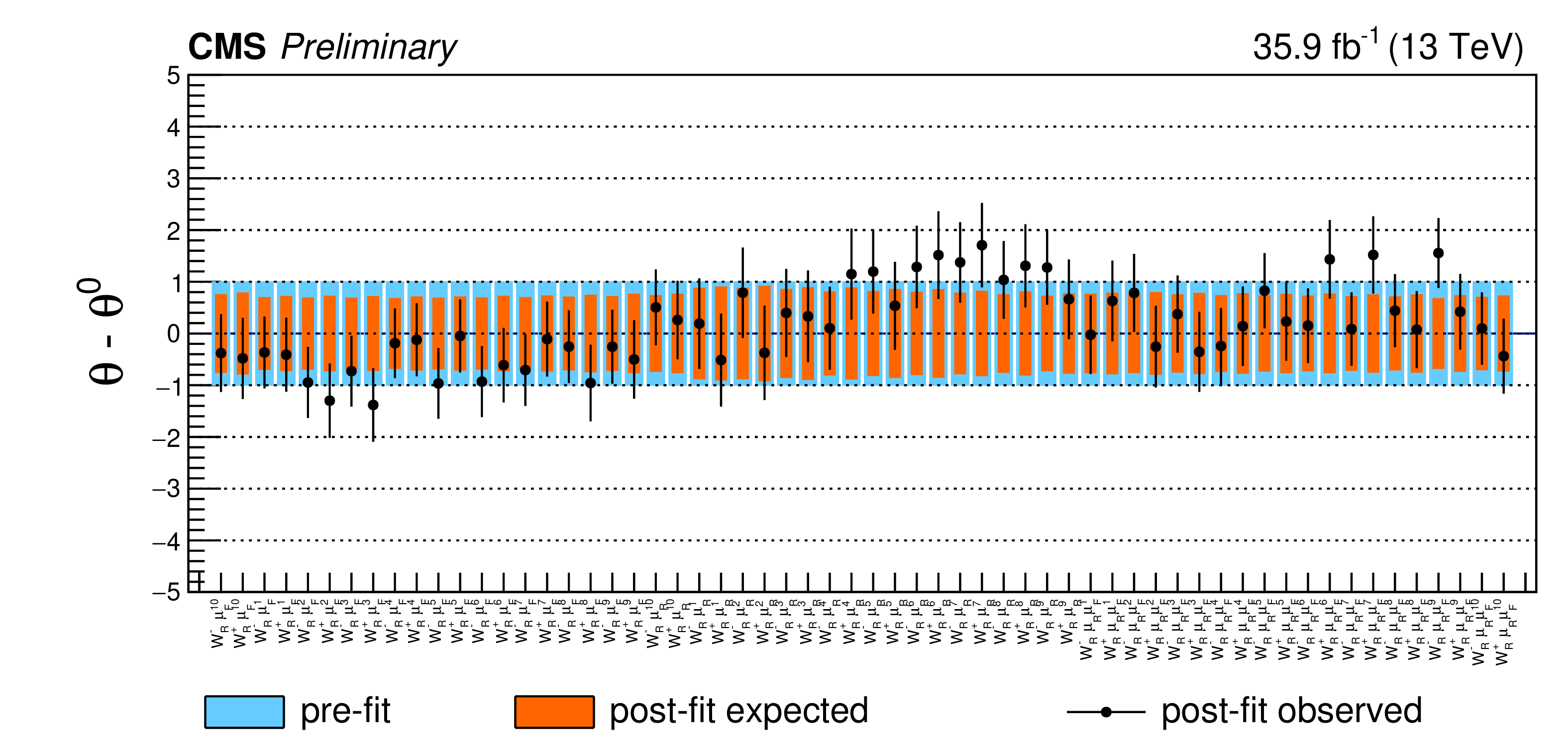
Figure 21:
Post-fit pulls and constraints of the nuisance parameters associated with the QCD scale systematics. The numbering refers to bins in the ${p_{\mathrm {T}} ^{\mathrm{W}}}$ spectrum in increasing order. The nuisance parameters applied to the "left'' polarization are shown on the left while the ones associated with the "right'' polarization are shown on the right. |
png pdf |
Figure 21-a:
Post-fit pulls and constraints of the nuisance parameters associated with the QCD scale systematics. The numbering refers to bins in the ${p_{\mathrm {T}} ^{\mathrm{W}}}$ spectrum in increasing order. The nuisance parameters applied to the "left'' polarization are shown on the left while the ones associated with the "right'' polarization are shown on the right. |
png pdf |
Figure 21-b:
Post-fit pulls and constraints of the nuisance parameters associated with the QCD scale systematics. The numbering refers to bins in the ${p_{\mathrm {T}} ^{\mathrm{W}}}$ spectrum in increasing order. The nuisance parameters applied to the "left'' polarization are shown on the left while the ones associated with the "right'' polarization are shown on the right. |
png pdf |
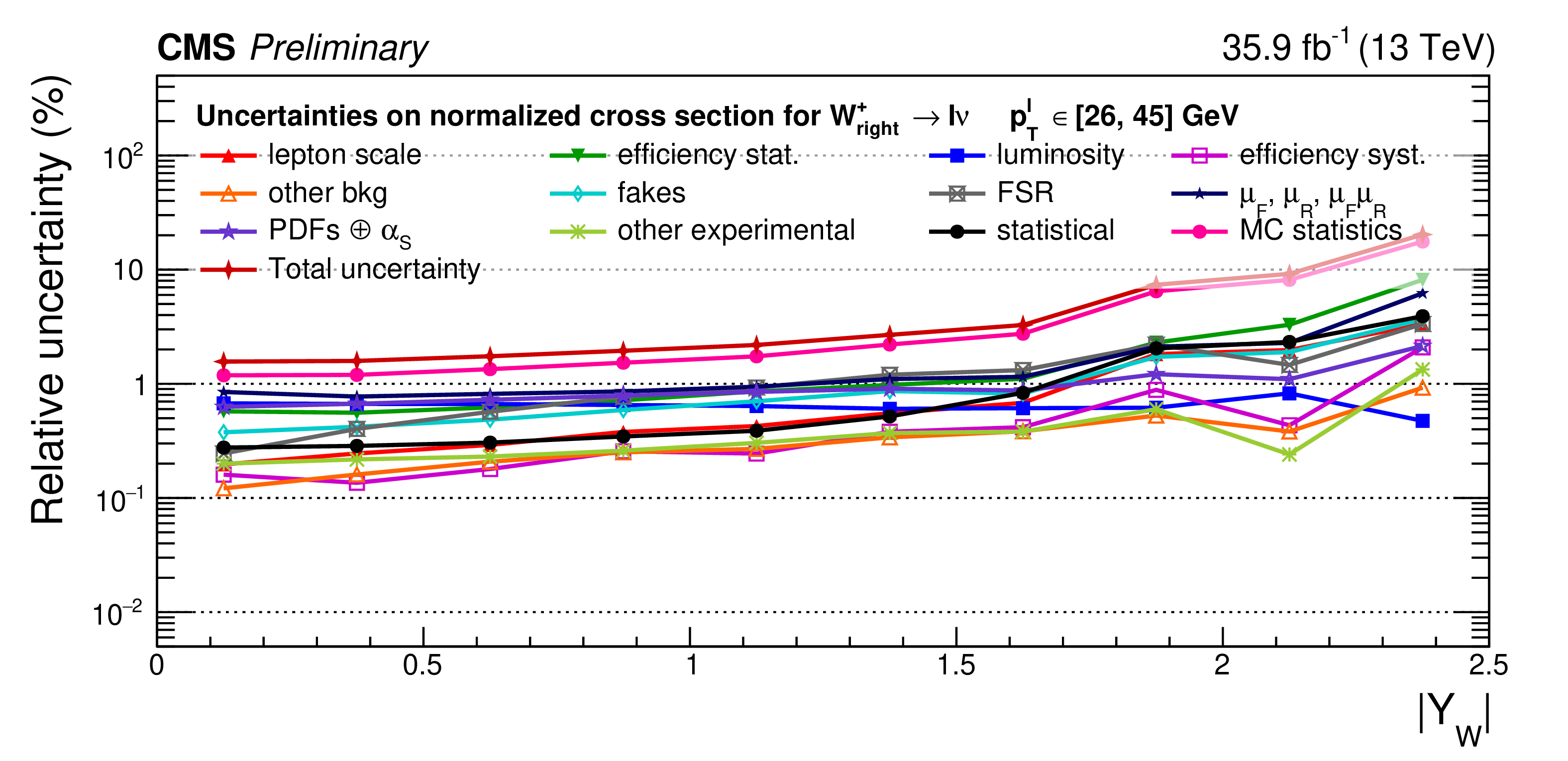
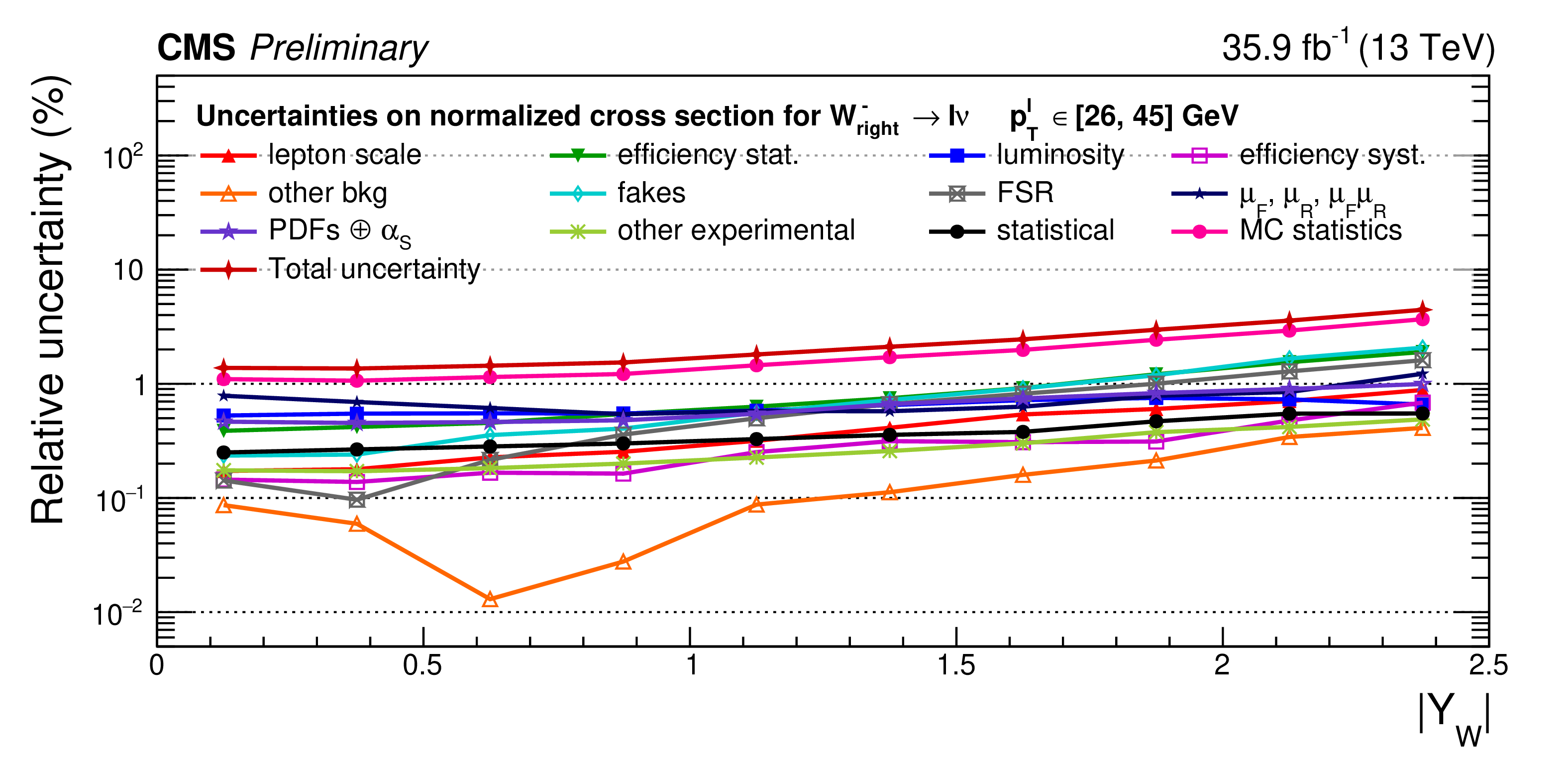
Figure 22:
Remaining impacts on the normalized polarized cross sections as a function of the rapidity. Shown are the impacts of the nuisance groups for $ {\mathrm{W^{+}} _{R}} $ (top), $ {\mathrm{W^{+}} _{L}} $ (middle), and $ {\mathrm{W^{-}} _{R}} $ (bottom). |
png pdf |
Figure 22-a:
Remaining impacts on the normalized polarized cross sections as a function of the rapidity. Shown are the impacts of the nuisance groups for $ {\mathrm{W^{+}} _{R}} $ (top), $ {\mathrm{W^{+}} _{L}} $ (middle), and $ {\mathrm{W^{-}} _{R}} $ (bottom). |

png pdf |
Figure 22-b:
Remaining impacts on the normalized polarized cross sections as a function of the rapidity. Shown are the impacts of the nuisance groups for $ {\mathrm{W^{+}} _{R}} $ (top), $ {\mathrm{W^{+}} _{L}} $ (middle), and $ {\mathrm{W^{-}} _{R}} $ (bottom). |
png pdf |
Figure 22-c:
Remaining impacts on the normalized polarized cross sections as a function of the rapidity. Shown are the impacts of the nuisance groups for $ {\mathrm{W^{+}} _{R}} $ (top), $ {\mathrm{W^{+}} _{L}} $ (middle), and $ {\mathrm{W^{-}} _{R}} $ (bottom). |

png pdf |
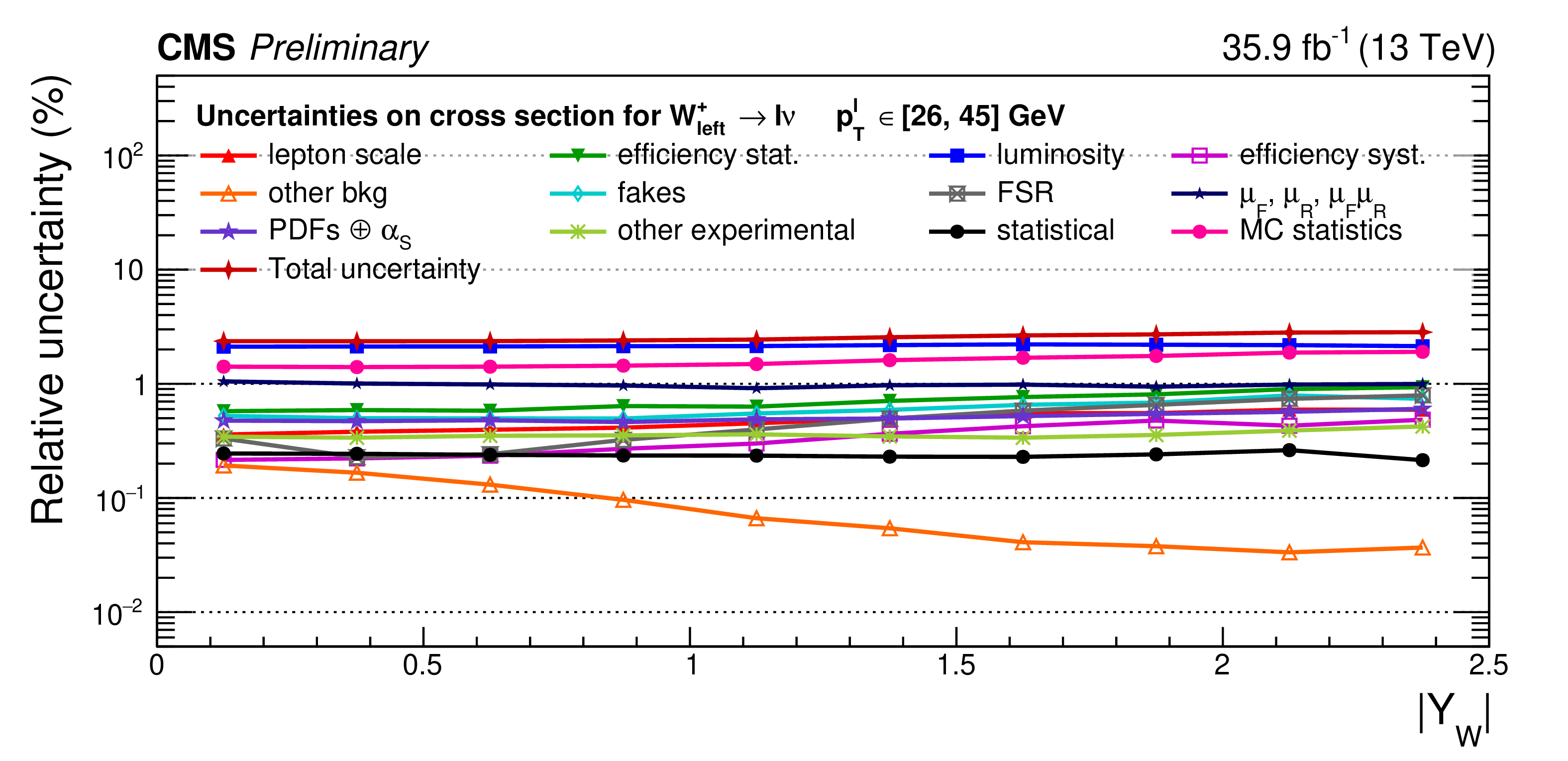
Figure 23:
Impacts on the absolute polarized cross sections as a function of the rapidity. Shown are the impacts of the nuisance groups for $ {\mathrm{W^{+}} _{L}} $ (top) and $ {\mathrm{W^{+}} _{R}} $ (bottom). |
png pdf |
Figure 23-a:
Impacts on the absolute polarized cross sections as a function of the rapidity. Shown are the impacts of the nuisance groups for $ {\mathrm{W^{+}} _{L}} $ (top) and $ {\mathrm{W^{+}} _{R}} $ (bottom). |
png pdf |
Figure 23-b:
Impacts on the absolute polarized cross sections as a function of the rapidity. Shown are the impacts of the nuisance groups for $ {\mathrm{W^{+}} _{L}} $ (top) and $ {\mathrm{W^{+}} _{R}} $ (bottom). |
png pdf |
Figure 24:
Impacts on the absolute polarized cross sections as a function of the rapidity. Shown are the impacts of the nuisance groups for $ {\mathrm{W^{-}} _{L}} $ (top) and $ {\mathrm{W^{-}} _{R}} $ (bottom). |
png pdf |
Figure 24-a:
Impacts on the absolute polarized cross sections as a function of the rapidity. Shown are the impacts of the nuisance groups for $ {\mathrm{W^{-}} _{L}} $ (top) and $ {\mathrm{W^{-}} _{R}} $ (bottom). |

png pdf |
Figure 24-b:
Impacts on the absolute polarized cross sections as a function of the rapidity. Shown are the impacts of the nuisance groups for $ {\mathrm{W^{-}} _{L}} $ (top) and $ {\mathrm{W^{-}} _{R}} $ (bottom). |

png pdf |
Figure 25:
Impacts on the charge asymmetry for $ {\mathrm{W} _{R}} $. |
png pdf |
Figure 26:
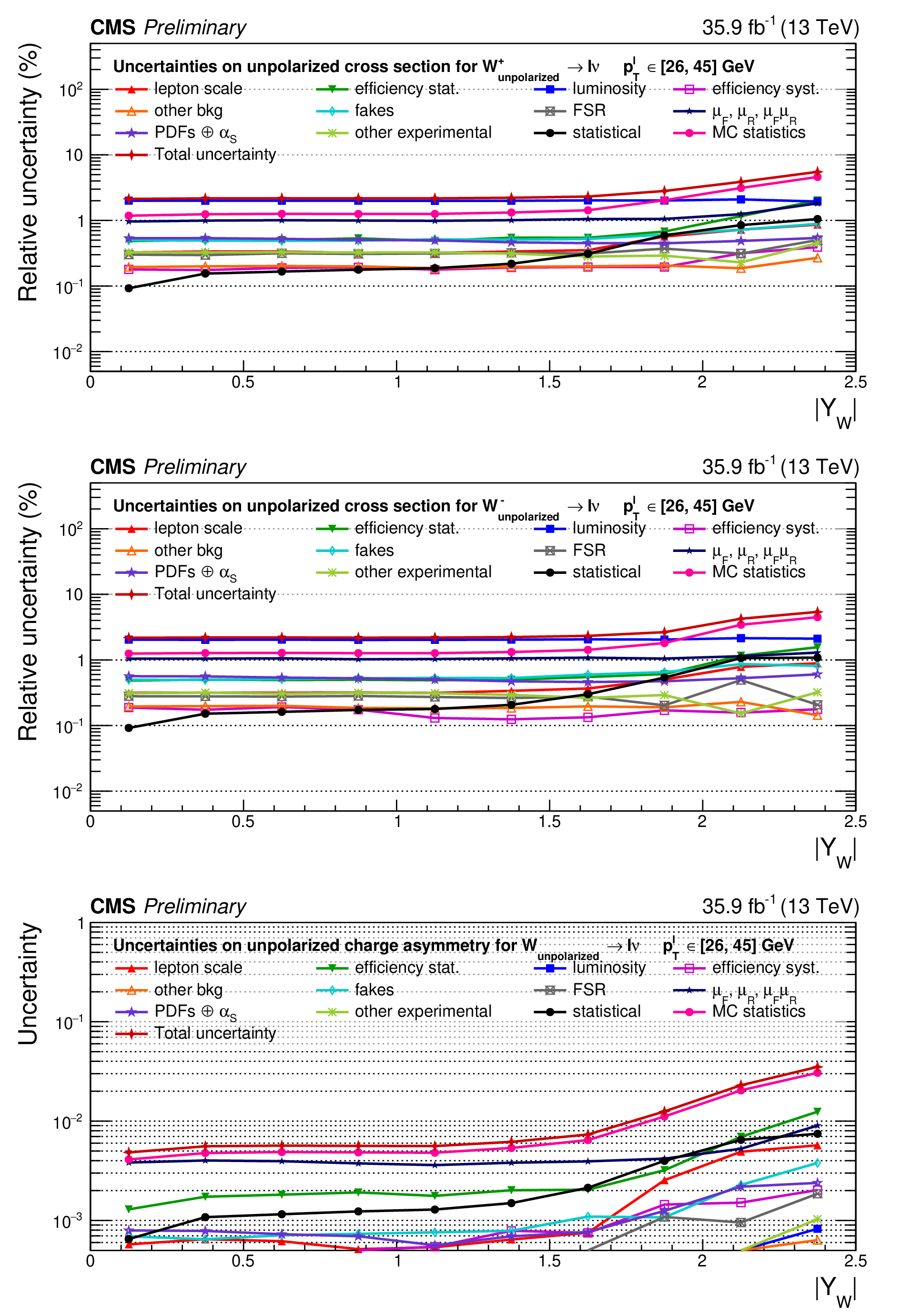
Impacts on the unpolarized absolute cross sections for $ {\mathrm{W^{+}}} $ (top), $ {\mathrm{W^{-}}} $ (middle), and the unpolarized charge asymmetry (bottom). |
png pdf |
Figure 26-a:
Impacts on the unpolarized absolute cross sections for $ {\mathrm{W^{+}}} $ (top), $ {\mathrm{W^{-}}} $ (middle), and the unpolarized charge asymmetry (bottom). |

png pdf |
Figure 26-b:
Impacts on the unpolarized absolute cross sections for $ {\mathrm{W^{+}}} $ (top), $ {\mathrm{W^{-}}} $ (middle), and the unpolarized charge asymmetry (bottom). |
png pdf |
Figure 26-c:
Impacts on the unpolarized absolute cross sections for $ {\mathrm{W^{+}}} $ (top), $ {\mathrm{W^{-}}} $ (middle), and the unpolarized charge asymmetry (bottom). |
png pdf |
Figure 27:
Impacts on the unpolarized normalized cross sections for $ {\mathrm{W^{+}}} $ (top) and $ {\mathrm{W^{-}}} $ (bottom). |

png pdf |
Figure 27-a:
Impacts on the unpolarized normalized cross sections for $ {\mathrm{W^{+}}} $ (top) and $ {\mathrm{W^{-}}} $ (bottom). |
png pdf |
Figure 27-b:
Impacts on the unpolarized normalized cross sections for $ {\mathrm{W^{+}}} $ (top) and $ {\mathrm{W^{-}}} $ (bottom). |
png pdf |
Figure 28:
Impacts on the A$_4$ coefficient as a function of $|Y_{\mathrm{W}}|$ for $ {\mathrm{W^{+}}} $ (top) and $ {\mathrm{W^{-}}} $ (bottom). |
png pdf |
Figure 28-a:
Impacts on the A$_4$ coefficient as a function of $|Y_{\mathrm{W}}|$ for $ {\mathrm{W^{+}}} $ (top) and $ {\mathrm{W^{-}}} $ (bottom). |
png pdf |
Figure 28-b:
Impacts on the A$_4$ coefficient as a function of $|Y_{\mathrm{W}}|$ for $ {\mathrm{W^{+}}} $ (top) and $ {\mathrm{W^{-}}} $ (bottom). |
png pdf |
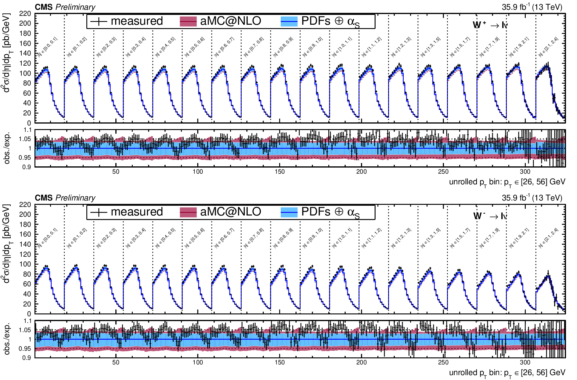
Figure 29:
Unrolled cross section for the combined electron+muon fit unrolled along ${{p_{\mathrm {T}}} ^{\ell}}$ in bins of ${| \eta ^{\ell} |}$ for ${\mathrm{W^{+}}}$ (top) and ${\mathrm{W^{-}}}$ (bottom). Shown in the colored bands are the prediction from MadGraph 5_aMC@NLO with the PDF+$\alpha _S$ variations in blue, and the total theoretical uncertainty in bordeaux. |
png pdf |
Figure 29-a:
Unrolled cross section for the combined electron+muon fit unrolled along ${{p_{\mathrm {T}}} ^{\ell}}$ in bins of ${| \eta ^{\ell} |}$ for ${\mathrm{W^{+}}}$ (top) and ${\mathrm{W^{-}}}$ (bottom). Shown in the colored bands are the prediction from MadGraph 5_aMC@NLO with the PDF+$\alpha _S$ variations in blue, and the total theoretical uncertainty in bordeaux. |

png pdf |
Figure 29-b:
Unrolled cross section for the combined electron+muon fit unrolled along ${{p_{\mathrm {T}}} ^{\ell}}$ in bins of ${| \eta ^{\ell} |}$ for ${\mathrm{W^{+}}}$ (top) and ${\mathrm{W^{-}}}$ (bottom). Shown in the colored bands are the prediction from MadGraph 5_aMC@NLO with the PDF+$\alpha _S$ variations in blue, and the total theoretical uncertainty in bordeaux. |
png pdf |
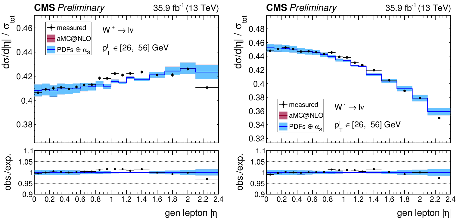
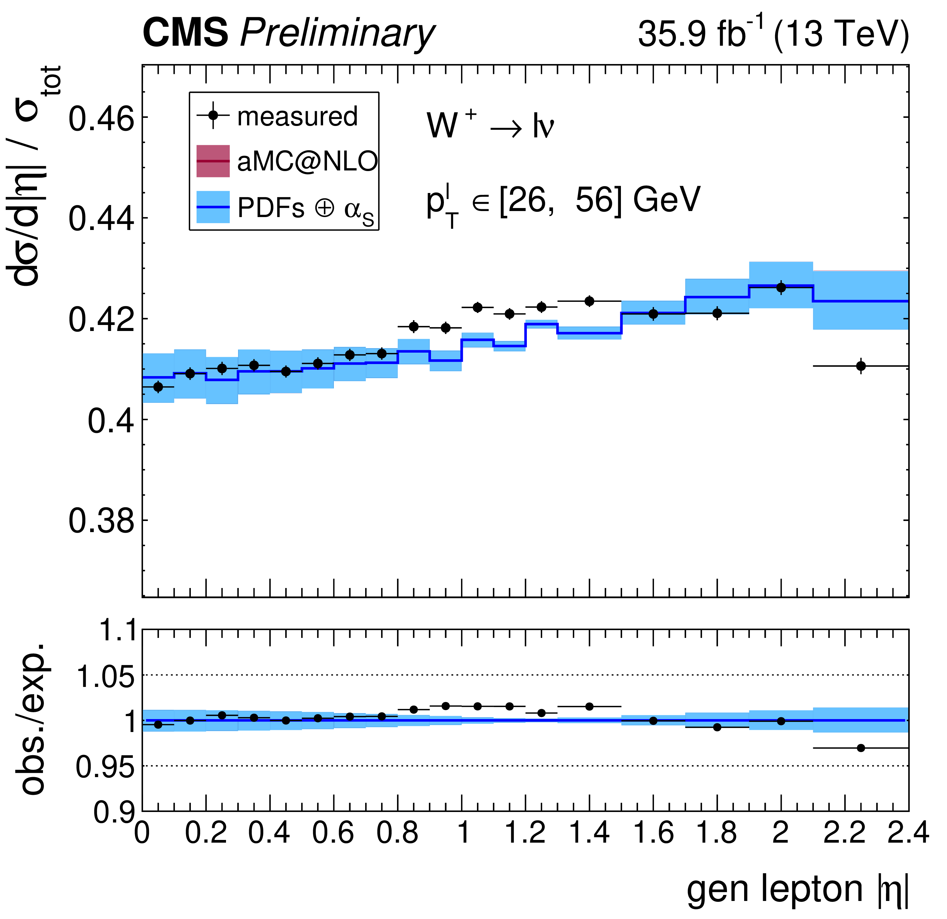
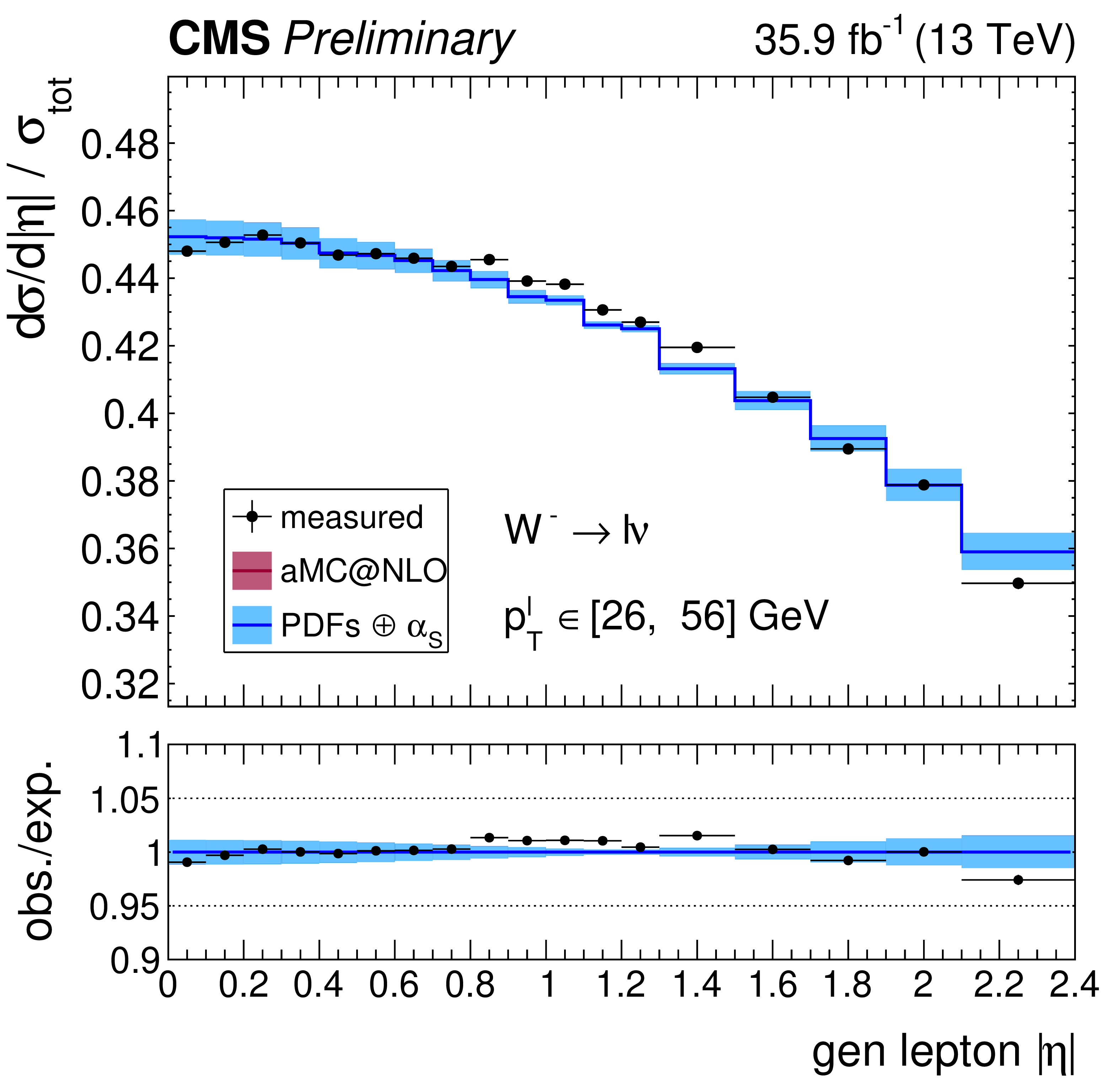
Figure 30:
Normalized cross sections as a function of ${| \eta ^{\ell} |}$, integrated over ${{p_{\mathrm {T}}} ^{\ell}}$ for ${\mathrm{W^{+}}}$ (left) and ${\mathrm{W^{-}}}$ (right). Shown in the colored bands are the prediction from MadGraph 5_aMC@NLO with the PDF+$\alpha _S$ variations in blue, and the total theoretical uncertainty in bordeaux. |
png pdf |
Figure 30-a:
Normalized cross sections as a function of ${| \eta ^{\ell} |}$, integrated over ${{p_{\mathrm {T}}} ^{\ell}}$ for ${\mathrm{W^{+}}}$ (left) and ${\mathrm{W^{-}}}$ (right). Shown in the colored bands are the prediction from MadGraph 5_aMC@NLO with the PDF+$\alpha _S$ variations in blue, and the total theoretical uncertainty in bordeaux. |
png pdf |
Figure 30-b:
Normalized cross sections as a function of ${| \eta ^{\ell} |}$, integrated over ${{p_{\mathrm {T}}} ^{\ell}}$ for ${\mathrm{W^{+}}}$ (left) and ${\mathrm{W^{-}}}$ (right). Shown in the colored bands are the prediction from MadGraph 5_aMC@NLO with the PDF+$\alpha _S$ variations in blue, and the total theoretical uncertainty in bordeaux. |
png pdf |
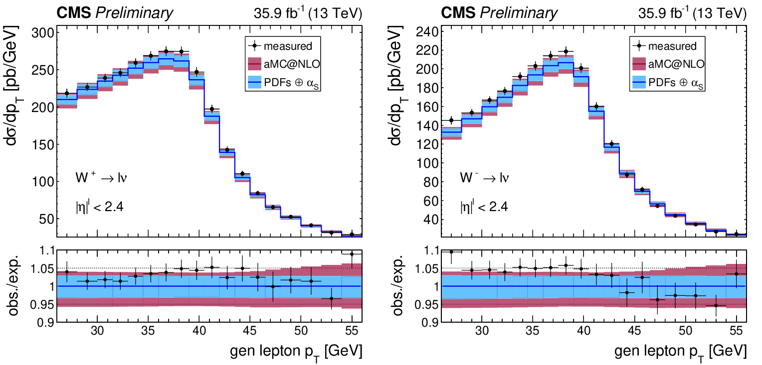
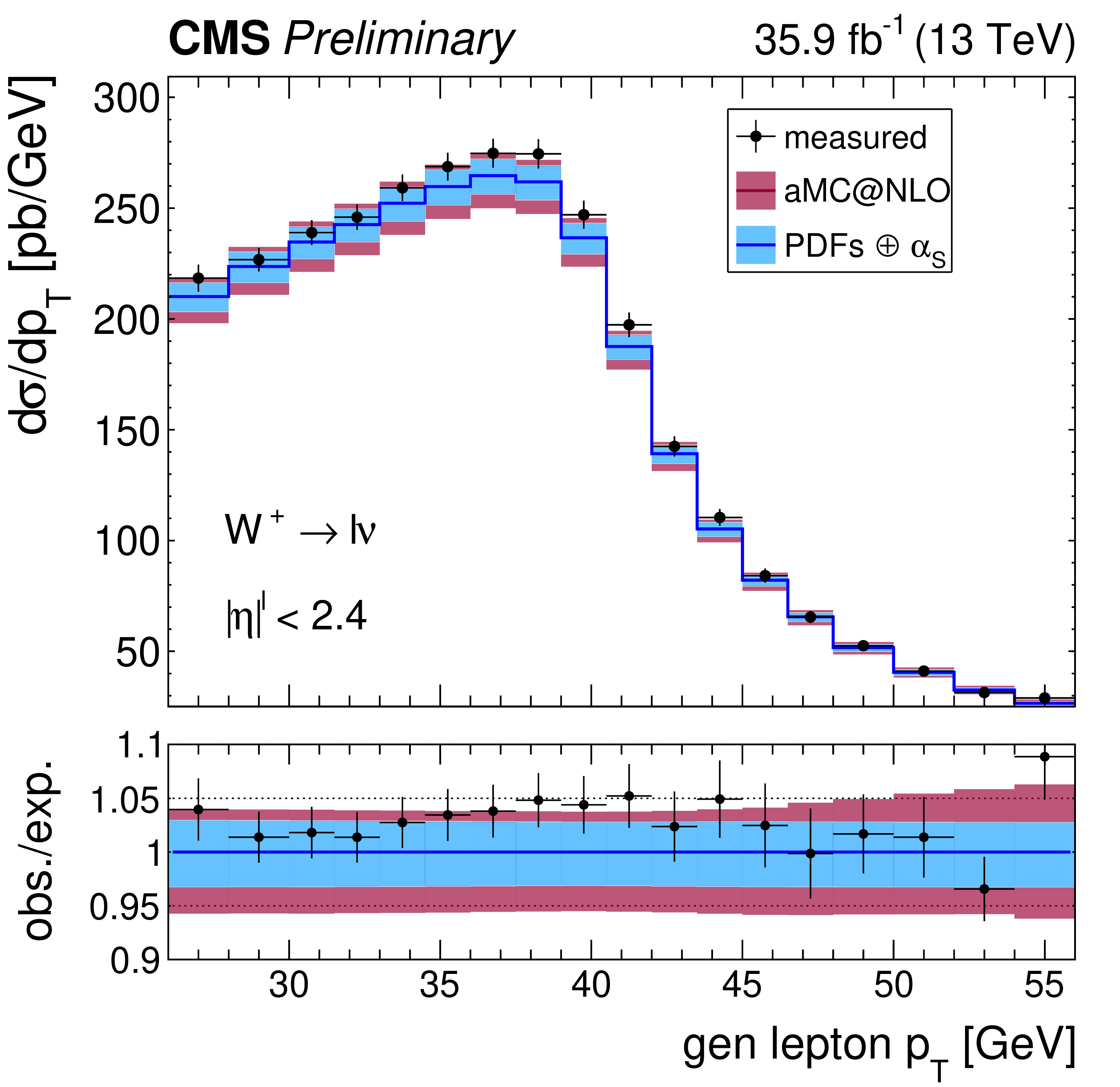
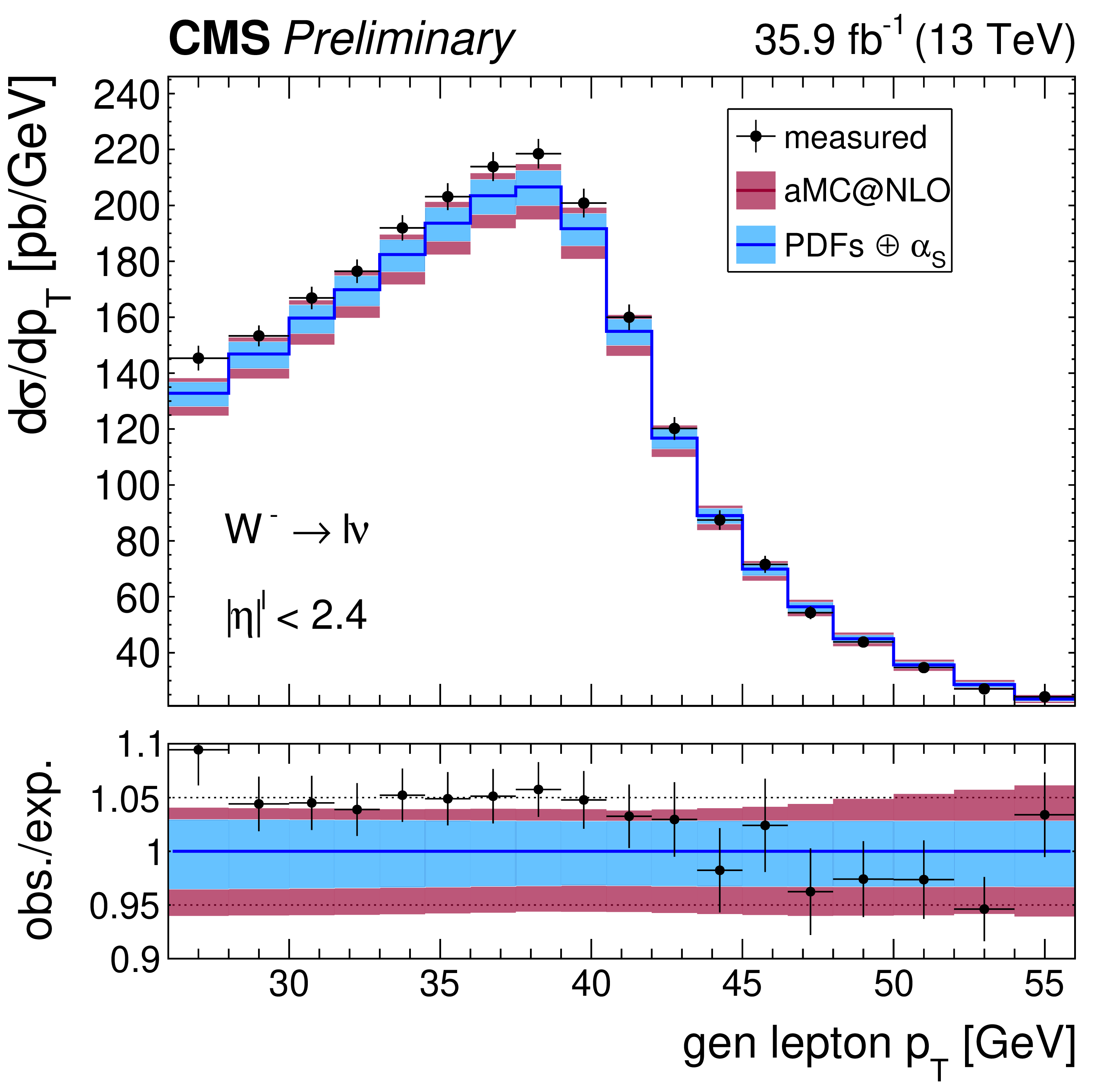
Figure 31:
Absolute cross sections as a function of ${{p_{\mathrm {T}}} ^{\ell}}$, integrated over ${| \eta ^{\ell} |}$ for ${\mathrm{W^{+}}}$ (left) and ${\mathrm{W^{-}}}$ (right). Shown in the colored bands are the prediction from MadGraph 5_aMC@NLO with the PDF+$\alpha _S$ variations in blue, and the total theoretical uncertainty in bordeaux. |
png pdf |
Figure 31-a:
Absolute cross sections as a function of ${{p_{\mathrm {T}}} ^{\ell}}$, integrated over ${| \eta ^{\ell} |}$ for ${\mathrm{W^{+}}}$ (left) and ${\mathrm{W^{-}}}$ (right). Shown in the colored bands are the prediction from MadGraph 5_aMC@NLO with the PDF+$\alpha _S$ variations in blue, and the total theoretical uncertainty in bordeaux. |
png pdf |
Figure 31-b:
Absolute cross sections as a function of ${{p_{\mathrm {T}}} ^{\ell}}$, integrated over ${| \eta ^{\ell} |}$ for ${\mathrm{W^{+}}}$ (left) and ${\mathrm{W^{-}}}$ (right). Shown in the colored bands are the prediction from MadGraph 5_aMC@NLO with the PDF+$\alpha _S$ variations in blue, and the total theoretical uncertainty in bordeaux. |
png pdf |
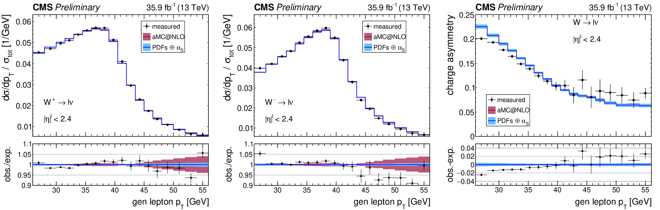
Figure 32:
Normalized cross sections as a function of ${{p_{\mathrm {T}}} ^{\ell}}$, integrated over ${| \eta ^{\ell} |}$ for ${\mathrm{W^{+}}}$ (left) and ${\mathrm{W^{-}}}$ (middle), and the resulting charge asymmetry (right). Shown in the colored bands are the prediction from MadGraph 5_aMC@NLO with the PDF+$\alpha _S$ variations in blue, and the total theoretical uncertainty in bordeaux. |

png pdf |
Figure 32-a:
Normalized cross sections as a function of ${{p_{\mathrm {T}}} ^{\ell}}$, integrated over ${| \eta ^{\ell} |}$ for ${\mathrm{W^{+}}}$ (left) and ${\mathrm{W^{-}}}$ (middle), and the resulting charge asymmetry (right). Shown in the colored bands are the prediction from MadGraph 5_aMC@NLO with the PDF+$\alpha _S$ variations in blue, and the total theoretical uncertainty in bordeaux. |

png pdf |
Figure 32-b:
Normalized cross sections as a function of ${{p_{\mathrm {T}}} ^{\ell}}$, integrated over ${| \eta ^{\ell} |}$ for ${\mathrm{W^{+}}}$ (left) and ${\mathrm{W^{-}}}$ (middle), and the resulting charge asymmetry (right). Shown in the colored bands are the prediction from MadGraph 5_aMC@NLO with the PDF+$\alpha _S$ variations in blue, and the total theoretical uncertainty in bordeaux. |

png pdf |
Figure 32-c:
Normalized cross sections as a function of ${{p_{\mathrm {T}}} ^{\ell}}$, integrated over ${| \eta ^{\ell} |}$ for ${\mathrm{W^{+}}}$ (left) and ${\mathrm{W^{-}}}$ (middle), and the resulting charge asymmetry (right). Shown in the colored bands are the prediction from MadGraph 5_aMC@NLO with the PDF+$\alpha _S$ variations in blue, and the total theoretical uncertainty in bordeaux. |
png pdf |
Figure 33:
Remaining impacts of the nuisance groups on the normalized cross sections as a function of ${| \eta ^{\ell} |}$, integrated in ${{p_{\mathrm {T}}} ^{\ell}}$, for ${\mathrm{W^{-}}}$. |
png pdf |
Figure 34:
Remaining impacts of the nuisance groups on the absolute cross sections as a function of ${| \eta ^{\ell} |}$, integrated in ${{p_{\mathrm {T}}} ^{\ell}}$, for ${\mathrm{W^{+}}}$ (top) and ${\mathrm{W^{-}}}$ (bottom). |
png pdf |
Figure 34-a:
Remaining impacts of the nuisance groups on the absolute cross sections as a function of ${| \eta ^{\ell} |}$, integrated in ${{p_{\mathrm {T}}} ^{\ell}}$, for ${\mathrm{W^{+}}}$ (top) and ${\mathrm{W^{-}}}$ (bottom). |
png pdf |
Figure 34-b:
Remaining impacts of the nuisance groups on the absolute cross sections as a function of ${| \eta ^{\ell} |}$, integrated in ${{p_{\mathrm {T}}} ^{\ell}}$, for ${\mathrm{W^{+}}}$ (top) and ${\mathrm{W^{-}}}$ (bottom). |
png pdf |
Figure 35:
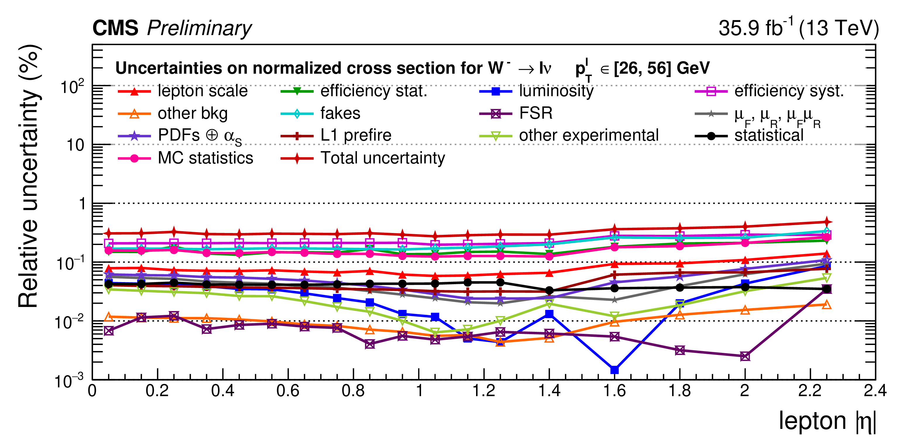
Remaining impacts of the nuisance groups on the normalized cross sections as a function of ${{p_{\mathrm {T}}} ^{\ell}}$, integrated over ${| \eta ^{\ell} |}$, for ${\mathrm{W^{+}}}$ (top), ${\mathrm{W^{-}}}$ (middle), and the resulting charge asymmetry (bottom). |
png pdf |
Figure 35-a:
Remaining impacts of the nuisance groups on the normalized cross sections as a function of ${{p_{\mathrm {T}}} ^{\ell}}$, integrated over ${| \eta ^{\ell} |}$, for ${\mathrm{W^{+}}}$ (top), ${\mathrm{W^{-}}}$ (middle), and the resulting charge asymmetry (bottom). |
png pdf |
Figure 35-b:
Remaining impacts of the nuisance groups on the normalized cross sections as a function of ${{p_{\mathrm {T}}} ^{\ell}}$, integrated over ${| \eta ^{\ell} |}$, for ${\mathrm{W^{+}}}$ (top), ${\mathrm{W^{-}}}$ (middle), and the resulting charge asymmetry (bottom). |
png pdf |
Figure 35-c:
Remaining impacts of the nuisance groups on the normalized cross sections as a function of ${{p_{\mathrm {T}}} ^{\ell}}$, integrated over ${| \eta ^{\ell} |}$, for ${\mathrm{W^{+}}}$ (top), ${\mathrm{W^{-}}}$ (middle), and the resulting charge asymmetry (bottom). |
png pdf |
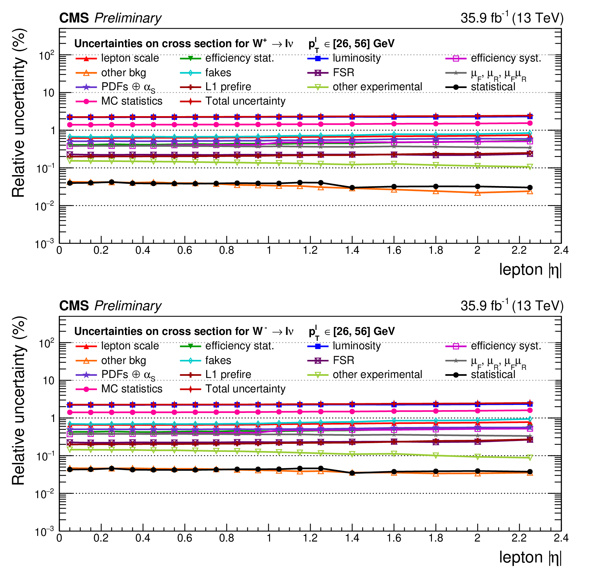
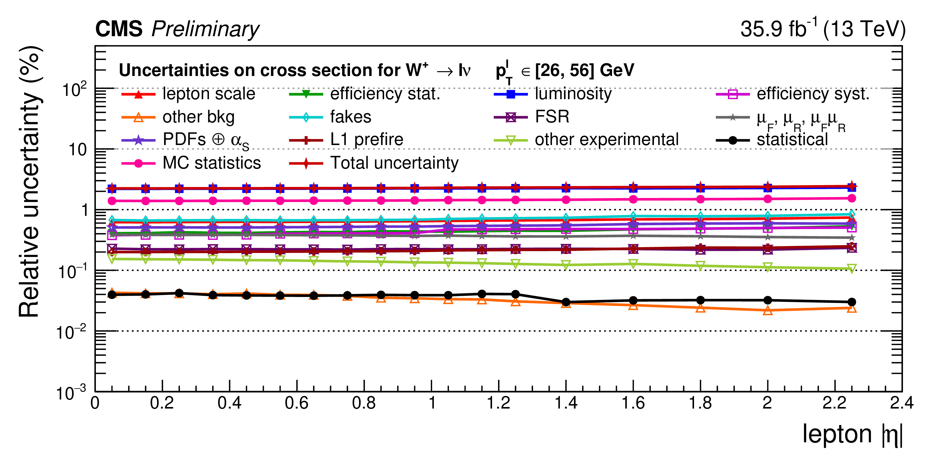
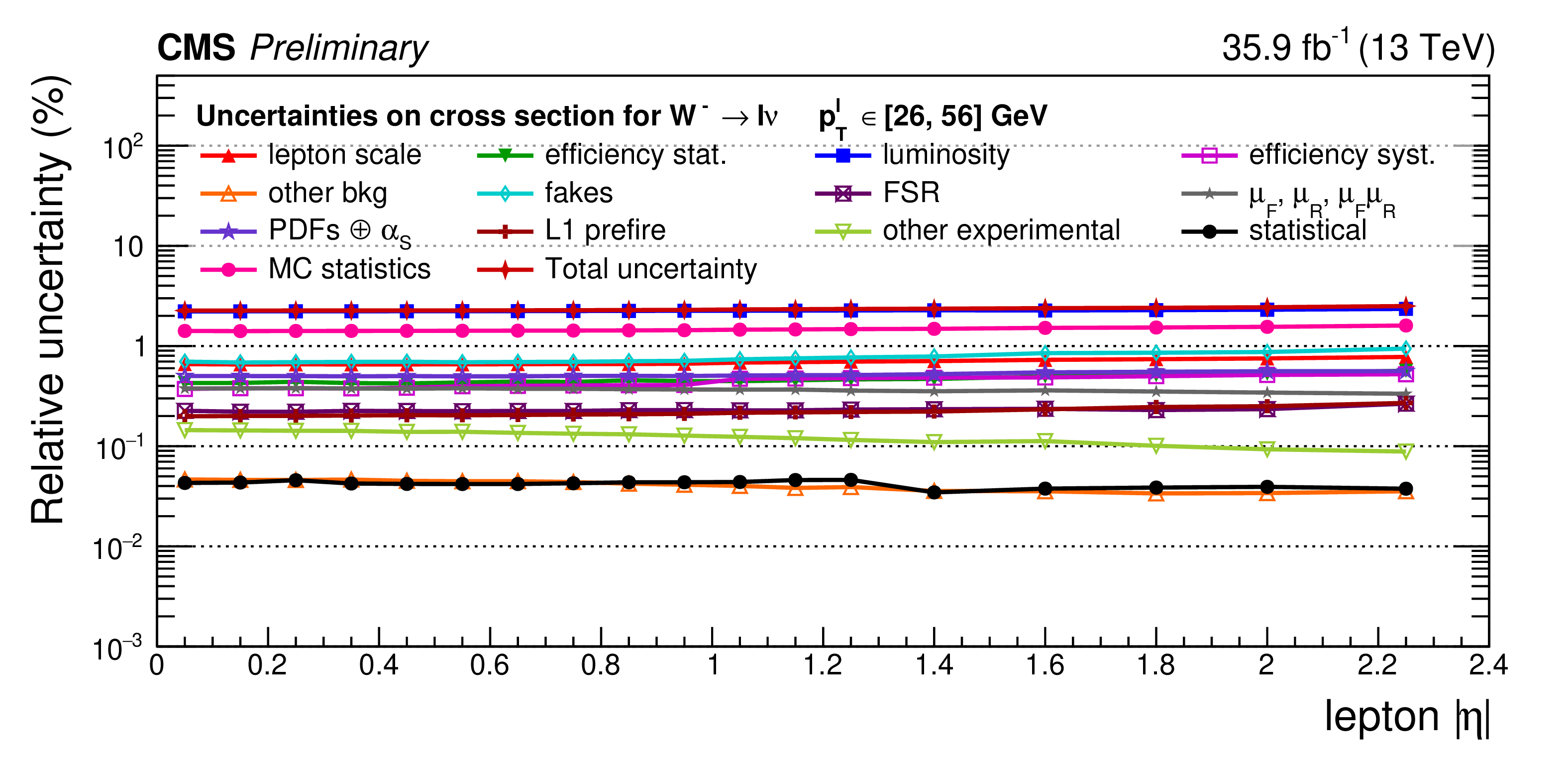
Figure 36:
Remaining impacts of the nuisance groups on the absolute cross sections as a function of ${{p_{\mathrm {T}}} ^{\ell}}$, integrated over ${| \eta ^{\ell} |}$, for ${\mathrm{W^{+}}}$ (top) and ${\mathrm{W^{-}}}$ (bottom). |
png pdf |
Figure 36-a:
Remaining impacts of the nuisance groups on the absolute cross sections as a function of ${{p_{\mathrm {T}}} ^{\ell}}$, integrated over ${| \eta ^{\ell} |}$, for ${\mathrm{W^{+}}}$ (top) and ${\mathrm{W^{-}}}$ (bottom). |

png pdf |
Figure 36-b:
Remaining impacts of the nuisance groups on the absolute cross sections as a function of ${{p_{\mathrm {T}}} ^{\ell}}$, integrated over ${| \eta ^{\ell} |}$, for ${\mathrm{W^{+}}}$ (top) and ${\mathrm{W^{-}}}$ (bottom). |
| Tables | |
png pdf |
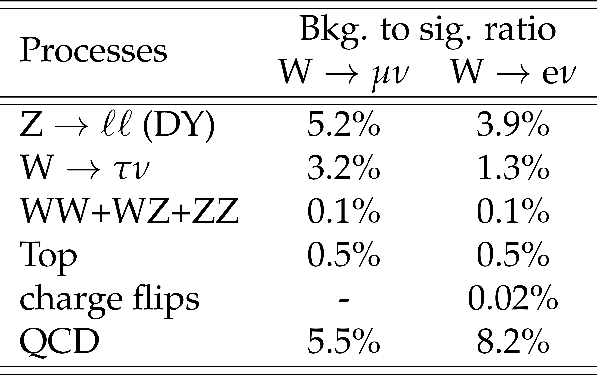
Table 1:
Estimated background-to-signal ratios in the $\mathrm{W} \to \mu \nu $ and $\mathrm{W} \to \mathrm{e} \nu $ channels. The DY simulation includes $\ell =$ e, $\mu$, $\tau $. |

png pdf |
Table 2:
Systematic uncertainties for each source and process. Quoted numbers correspond to the size of log-normal nuisance parameters applied in the fit, while a "yes'' in a given cell corresponds to the given systematic uncertainty being applied as a shape variation over the full 2D template space. |
| Summary |
|
A differential measurement of the W boson cross sections, measured as a function of the W boson rapidity, ${| Y_{\mathrm{W}} |} $, and for the two charges separately, ${\mathrm{W^{+}}} \to \ell^+\nu$ and ${\mathrm{W^{-}}} \to \ell^-\bar\nu$, is presented by the CMS Collaboration. Double-differential cross section measurements of the W boson are presented as a function of the charged lepton transverse momentum, ${p_{\mathrm{T}}}^{\ell}$, and lepton pseudorapidity, $|\eta^{\ell}|$. For both measurements, the differential charge asymmetry is also presented. The measurement is based on data taken in pp collisions at the LHC at a center-of-mass energy of $\sqrt{s} = $ 13 TeV with an integrated luminosity of 35.9 fb$^{-1}$ . Differential cross sections are presented both absolute and normalized to the total production cross section within a given acceptance. For the helicity measurement, the range ${| Y_{\mathrm{W}} |} < $ 2.5 is considered, while for the double-differential cross section the range $|\eta^{\ell}| < $ 2.4 and 26 $ < p_{\mathrm{T}}^{\ell} < $ 55 GeV is used. The measurement is performed using both the muon and the electron channels, combined together considering all sources of correlated and uncorrelated uncertainties. The precision in the measurement as a function of ${| Y_{\mathrm{W}} |} $, using a combination of the two channels, is about 2% in central ${| Y_{\mathrm{W}} |}$ bins, and 5% to 20%, depending on the charge-polarization combination, in the outermost acceptance bins. The precision of the double-differential cross section, relative to the total, is about 1% in each of the 324 bins relative to the central part of the detector, $|\eta^{\ell}| < 1$, and better than 2.5% up to $|\eta^{\ell}| < 2$ for each of the two W charges. Charge asymmetries are also measured, differentially in ${| Y_{\mathrm{W}} |}$ and polarization, as well as in ${p_{\mathrm{T}}}^{\ell}$ and $|\eta^{\ell}|$. The uncertainties in these asymmetries range from 0.1% in high-acceptance regions to roughly 2.5% in regions of phase space with lower detector acceptance. This measurement is used to constrain PDF parameters in a simultaneous fit of the measurements from the two channels and the two W charges. The constraints are derived at detector level on 60 uncorrelated eigenvalues of the NNPDF3.0 set of PDFs within the MadGraph5+MCatNLO generator code, and show a total constraint down to $\simeq$70% of the pre-fit uncertainties for certain variations of the PDF nuisance parameters. |
| Additional Figures | |
png pdf |
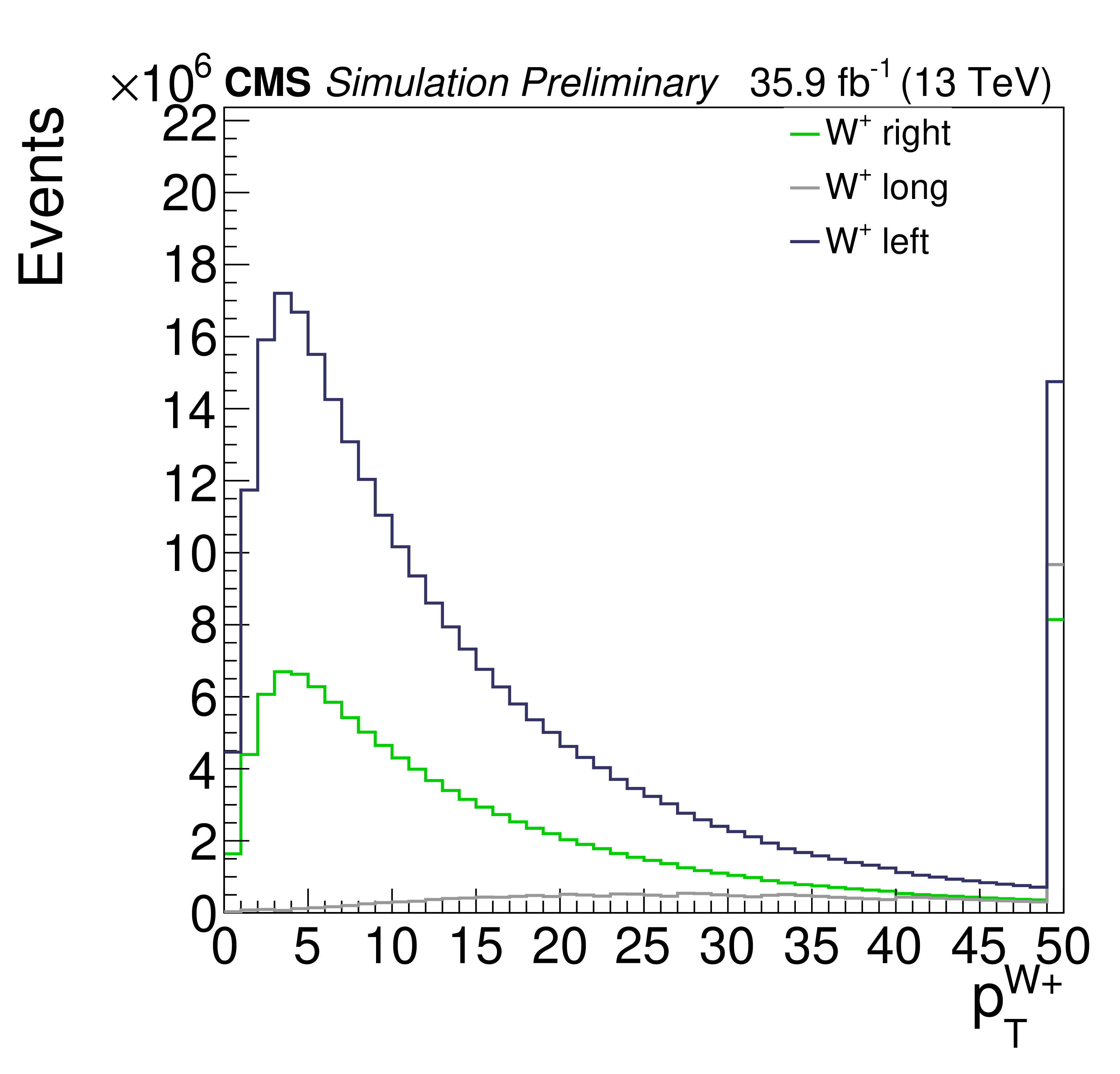
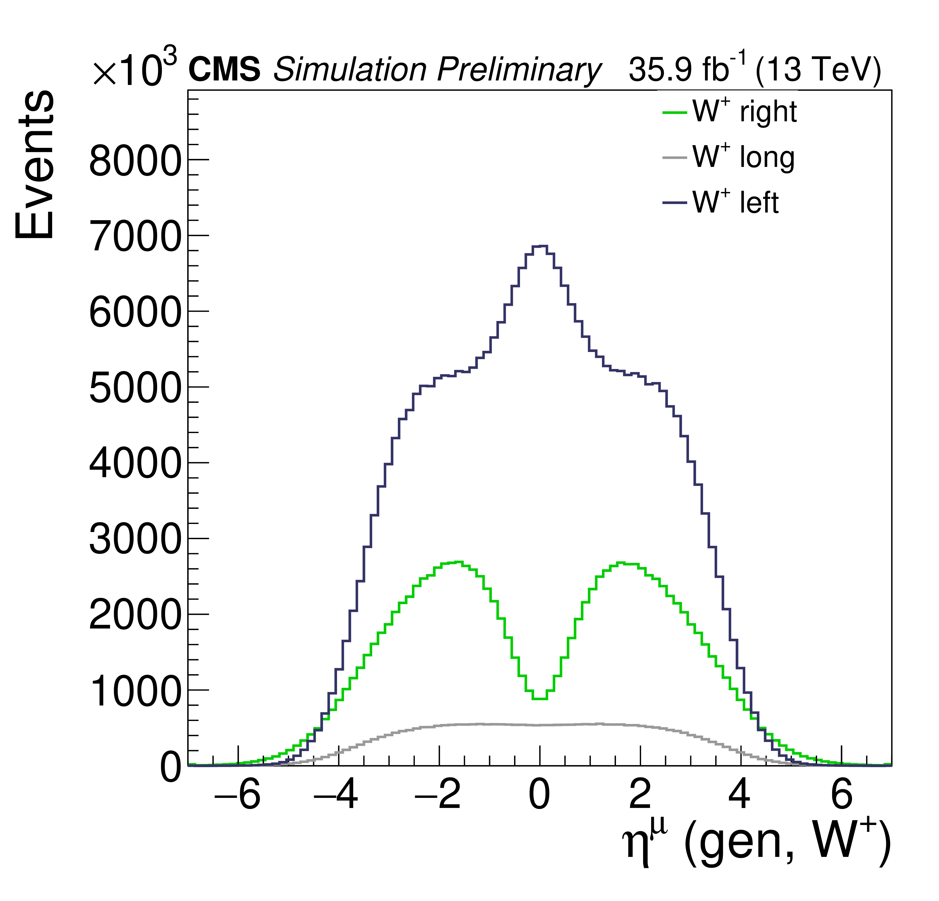
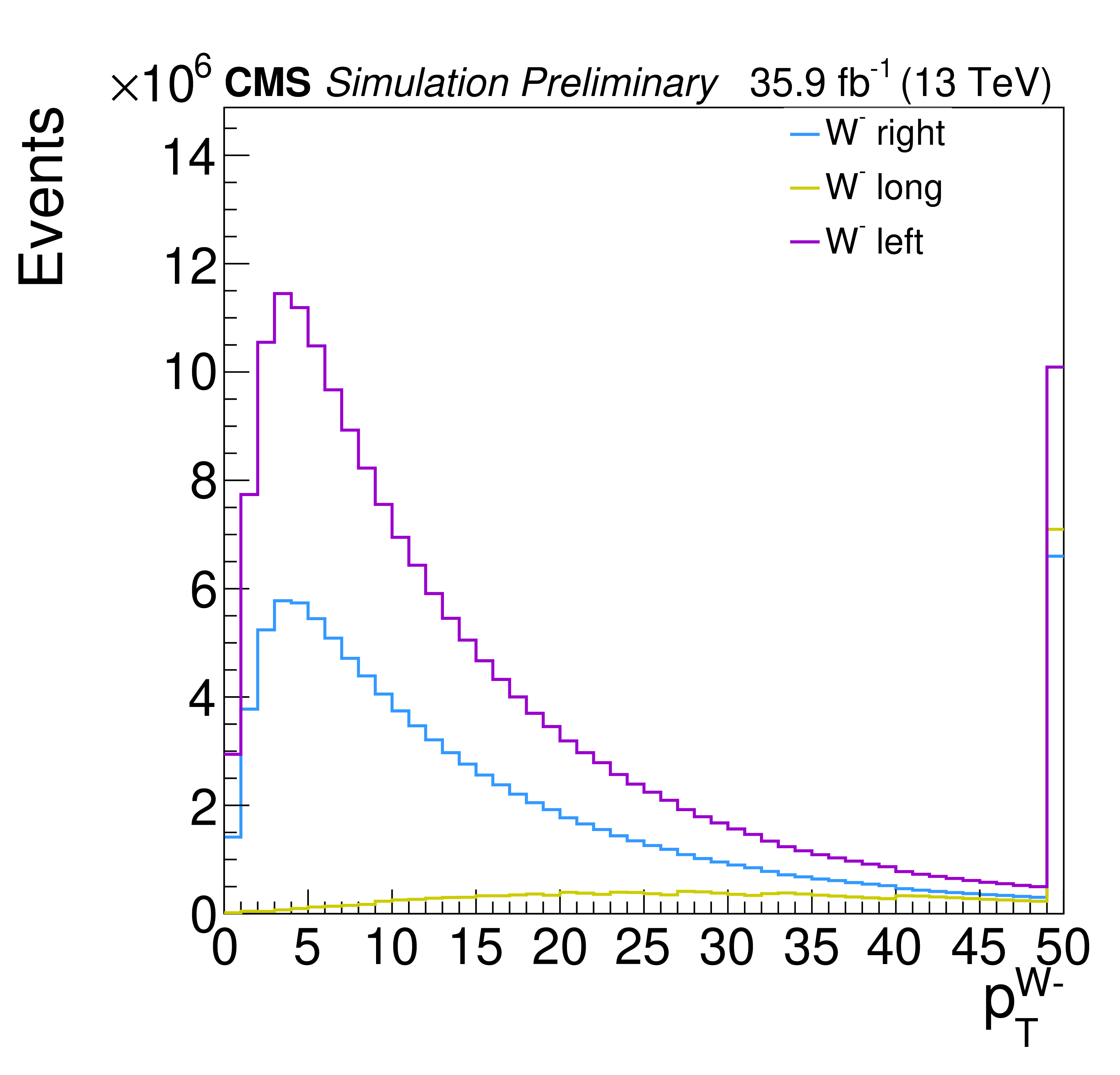
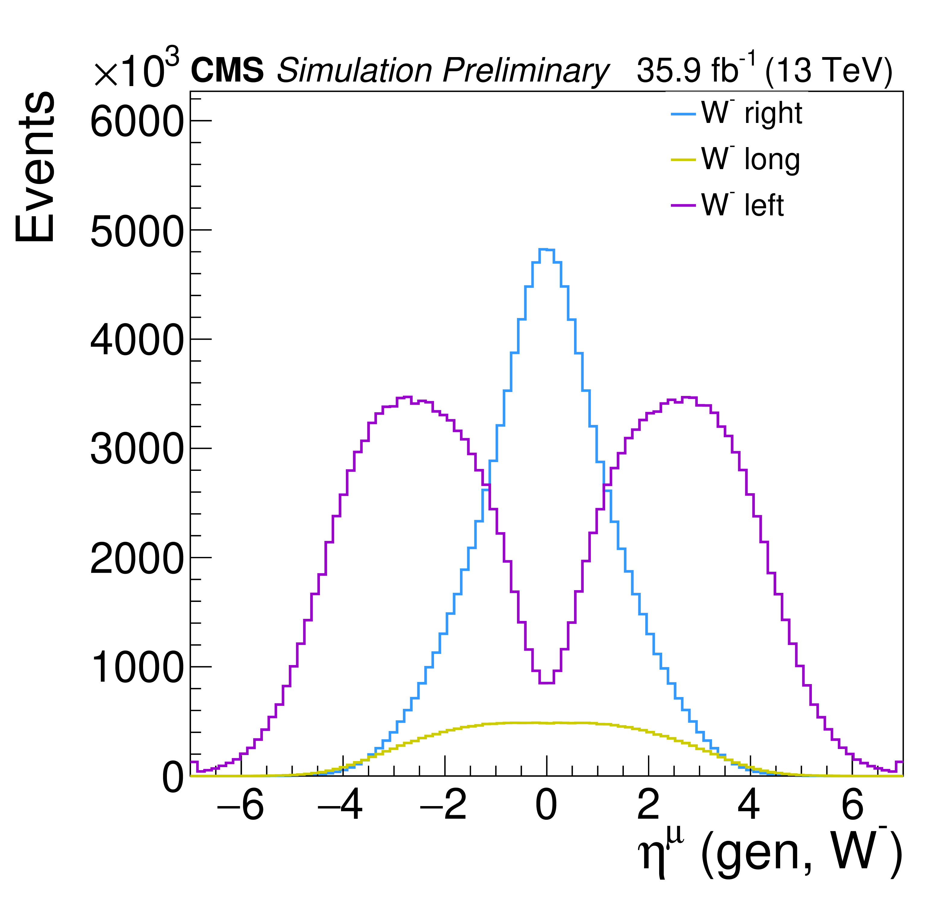
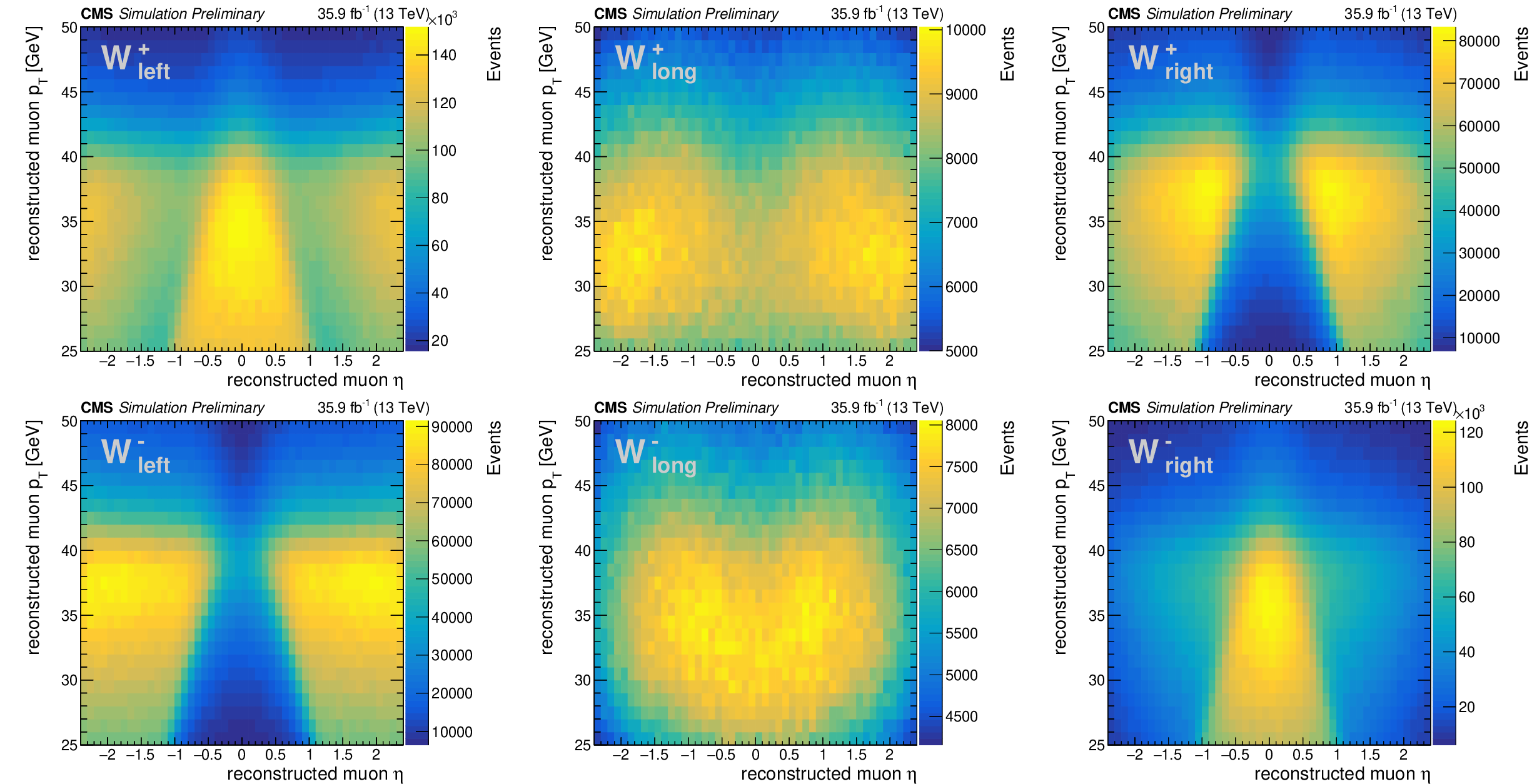
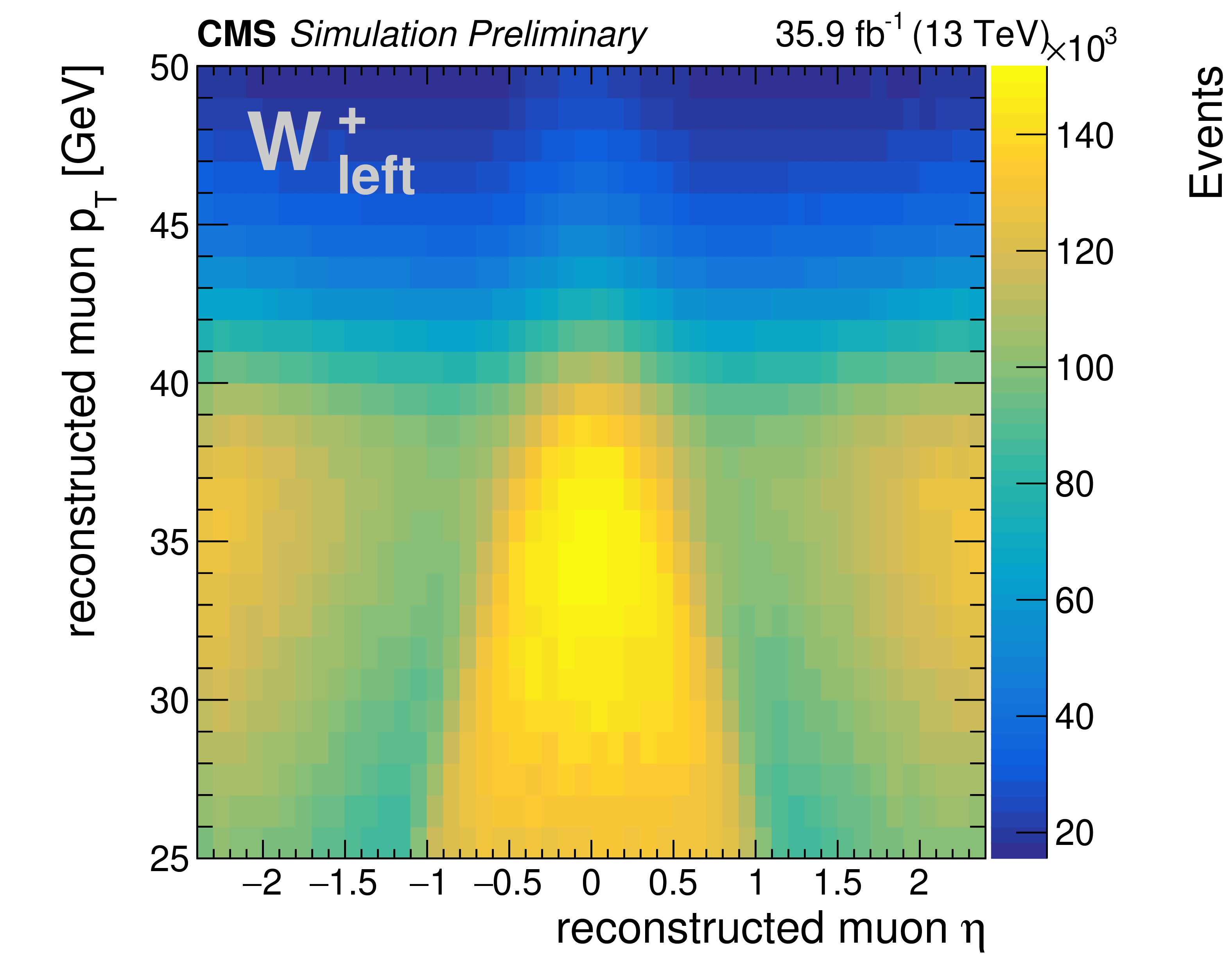
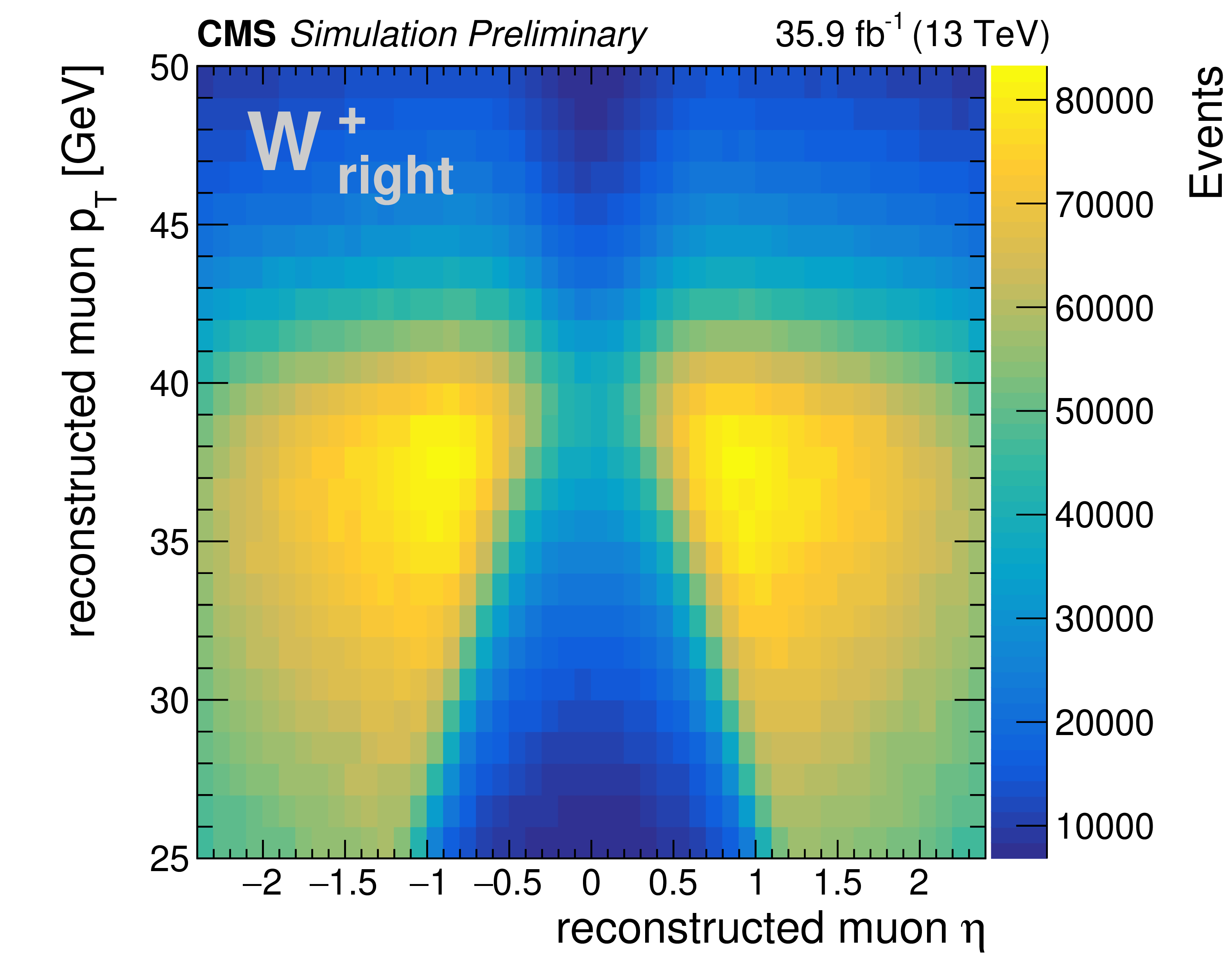
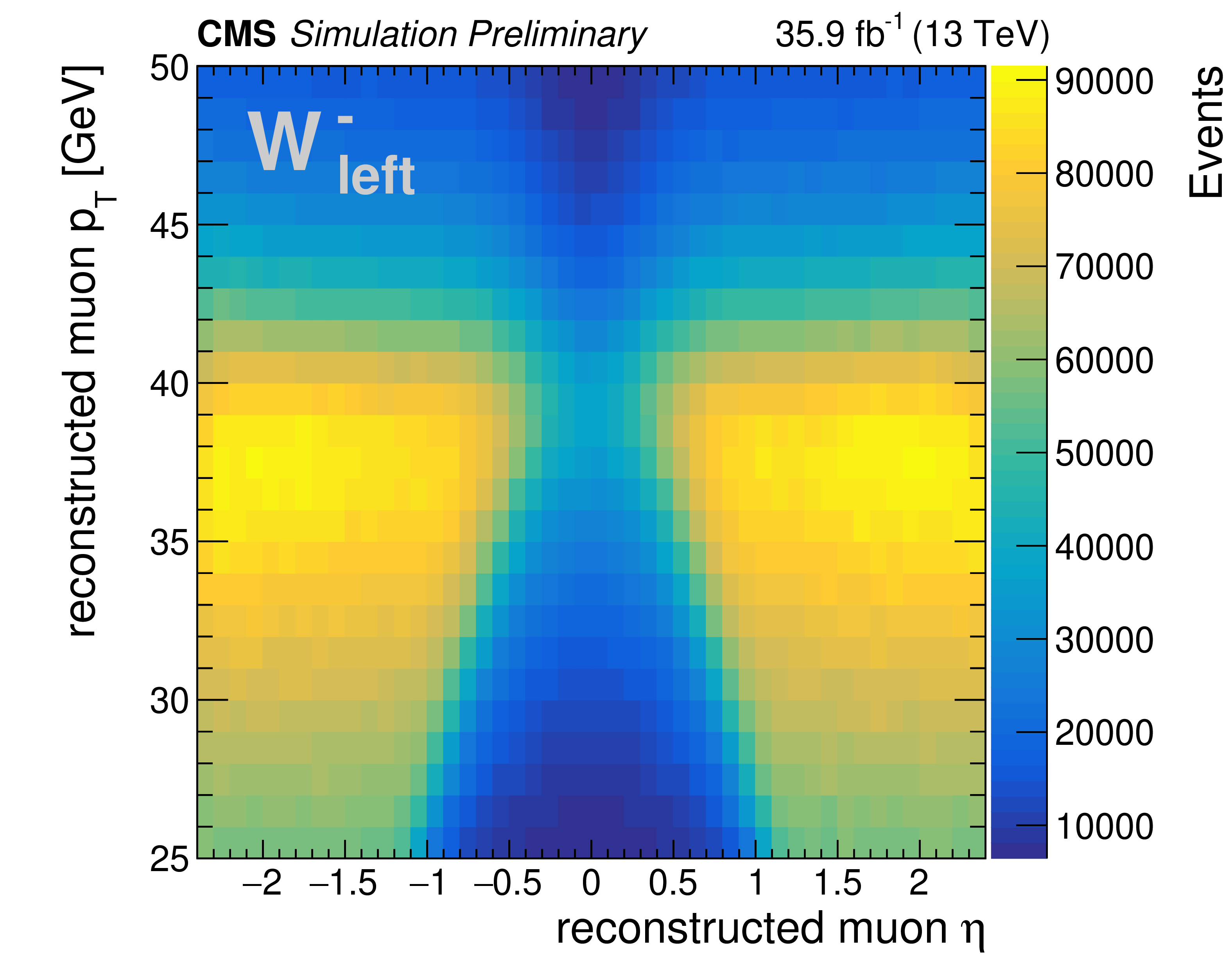
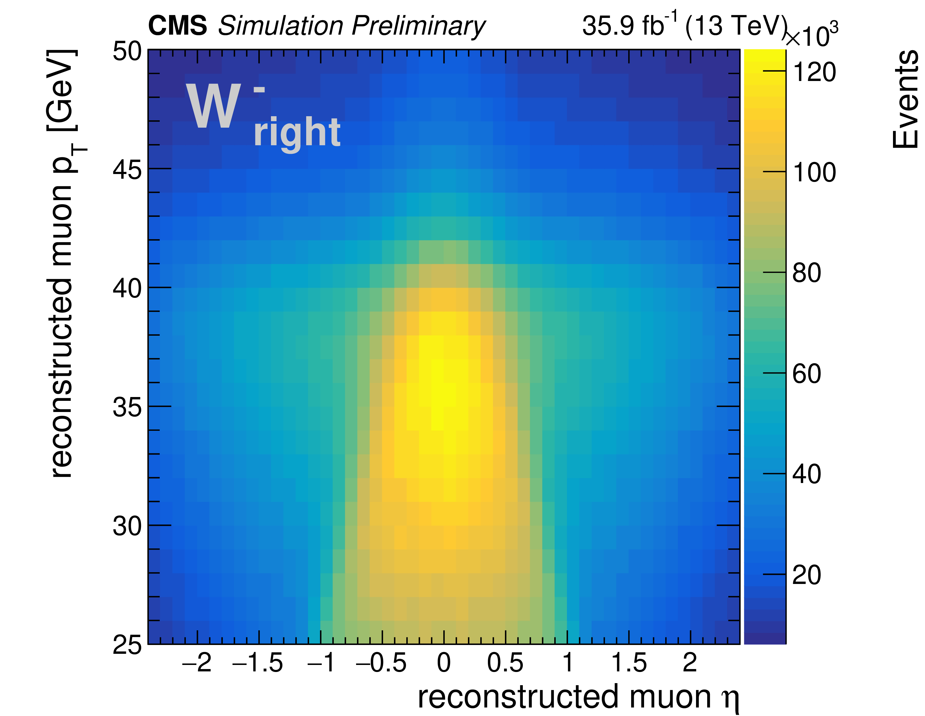
Additional Figure 1:
Distributions of $\eta $ and $p_{\mathrm{T}}$ of the reconstructed muon in W boson decays, split into W boson charge and polarisation (left, longitudinal, right). For a given charge and helicity state, the peculiar shape of each distribution is determined by the underlying W rapidity distribution, which in turn depends on the proton PDFs. These distributions are obtained from simulated $\mathrm{W}(\mu \nu )$+jets events at $\sqrt {s} = $ 13 TeV using MadGraph5\_aMC@NLO. Event yields are normalized to an integrated luminosity of 35.9 fb$^{-1}$. No event selection is applied, except for the requirement that a muon is identified and reconstructed within the CMS detector. |
png pdf |
Additional Figure 1-a:
Distributions of $\eta $ and $p_{\mathrm{T}}$ of the reconstructed muon in W boson decays, split into W boson charge and polarisation (left, longitudinal, right). For a given charge and helicity state, the peculiar shape of each distribution is determined by the underlying W rapidity distribution, which in turn depends on the proton PDFs. These distributions are obtained from simulated $\mathrm{W}(\mu \nu )$+jets events at $\sqrt {s} = $ 13 TeV using MadGraph5\_aMC@NLO. Event yields are normalized to an integrated luminosity of 35.9 fb$^{-1}$. No event selection is applied, except for the requirement that a muon is identified and reconstructed within the CMS detector. |

png pdf |
Additional Figure 1-b:
Distributions of $\eta $ and $p_{\mathrm{T}}$ of the reconstructed muon in W boson decays, split into W boson charge and polarisation (left, longitudinal, right). For a given charge and helicity state, the peculiar shape of each distribution is determined by the underlying W rapidity distribution, which in turn depends on the proton PDFs. These distributions are obtained from simulated $\mathrm{W}(\mu \nu )$+jets events at $\sqrt {s} = $ 13 TeV using MadGraph5\_aMC@NLO. Event yields are normalized to an integrated luminosity of 35.9 fb$^{-1}$. No event selection is applied, except for the requirement that a muon is identified and reconstructed within the CMS detector. |
png pdf |
Additional Figure 1-c:
Distributions of $\eta $ and $p_{\mathrm{T}}$ of the reconstructed muon in W boson decays, split into W boson charge and polarisation (left, longitudinal, right). For a given charge and helicity state, the peculiar shape of each distribution is determined by the underlying W rapidity distribution, which in turn depends on the proton PDFs. These distributions are obtained from simulated $\mathrm{W}(\mu \nu )$+jets events at $\sqrt {s} = $ 13 TeV using MadGraph5\_aMC@NLO. Event yields are normalized to an integrated luminosity of 35.9 fb$^{-1}$. No event selection is applied, except for the requirement that a muon is identified and reconstructed within the CMS detector. |
png pdf |
Additional Figure 1-d:
Distributions of $\eta $ and $p_{\mathrm{T}}$ of the reconstructed muon in W boson decays, split into W boson charge and polarisation (left, longitudinal, right). For a given charge and helicity state, the peculiar shape of each distribution is determined by the underlying W rapidity distribution, which in turn depends on the proton PDFs. These distributions are obtained from simulated $\mathrm{W}(\mu \nu )$+jets events at $\sqrt {s} = $ 13 TeV using MadGraph5\_aMC@NLO. Event yields are normalized to an integrated luminosity of 35.9 fb$^{-1}$. No event selection is applied, except for the requirement that a muon is identified and reconstructed within the CMS detector. |

png pdf |
Additional Figure 1-e:
Distributions of $\eta $ and $p_{\mathrm{T}}$ of the reconstructed muon in W boson decays, split into W boson charge and polarisation (left, longitudinal, right). For a given charge and helicity state, the peculiar shape of each distribution is determined by the underlying W rapidity distribution, which in turn depends on the proton PDFs. These distributions are obtained from simulated $\mathrm{W}(\mu \nu )$+jets events at $\sqrt {s} = $ 13 TeV using MadGraph5\_aMC@NLO. Event yields are normalized to an integrated luminosity of 35.9 fb$^{-1}$. No event selection is applied, except for the requirement that a muon is identified and reconstructed within the CMS detector. |
png pdf |
Additional Figure 1-f:
Distributions of $\eta $ and $p_{\mathrm{T}}$ of the reconstructed muon in W boson decays, split into W boson charge and polarisation (left, longitudinal, right). For a given charge and helicity state, the peculiar shape of each distribution is determined by the underlying W rapidity distribution, which in turn depends on the proton PDFs. These distributions are obtained from simulated $\mathrm{W}(\mu \nu )$+jets events at $\sqrt {s} = $ 13 TeV using MadGraph5\_aMC@NLO. Event yields are normalized to an integrated luminosity of 35.9 fb$^{-1}$. No event selection is applied, except for the requirement that a muon is identified and reconstructed within the CMS detector. |

png pdf |
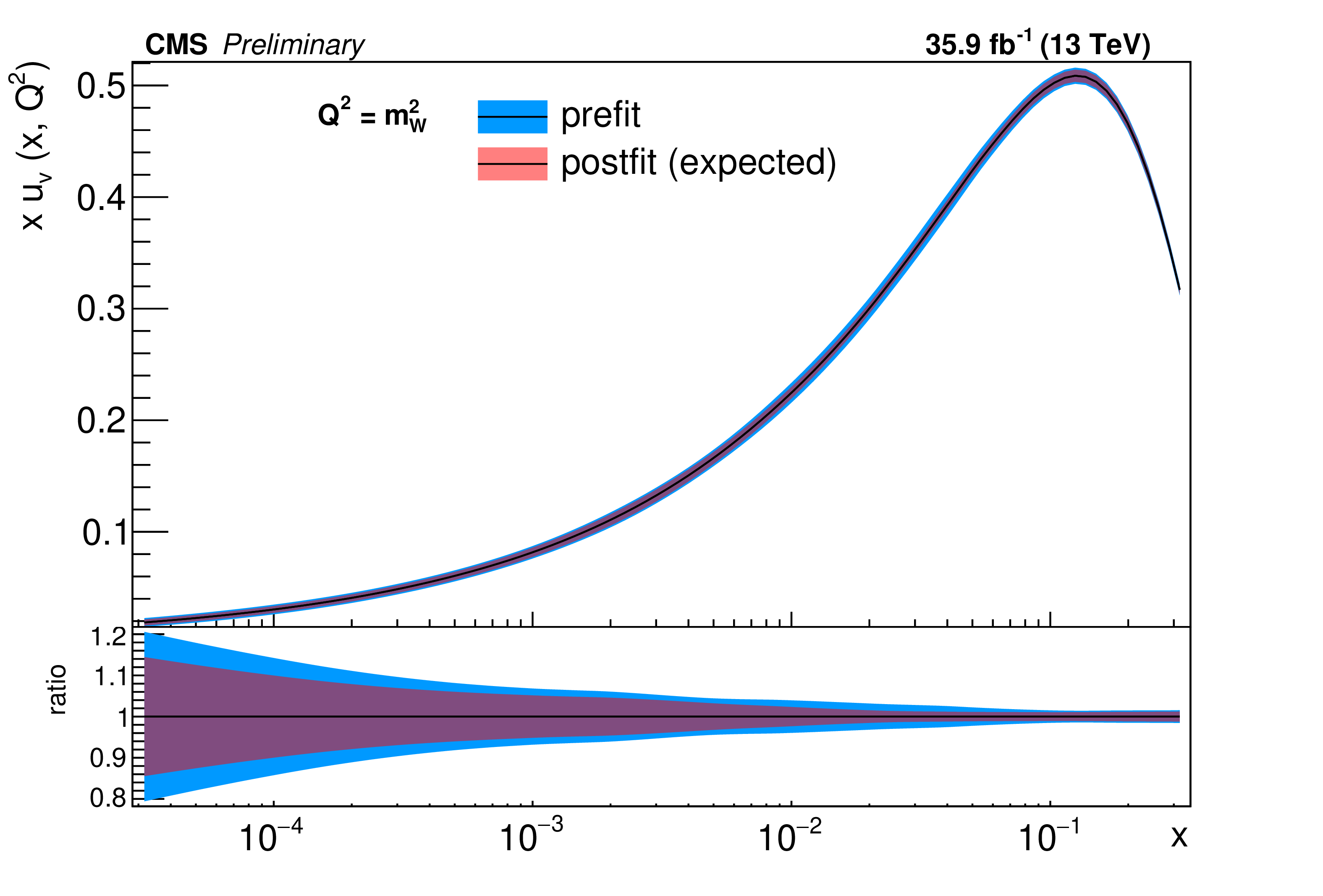
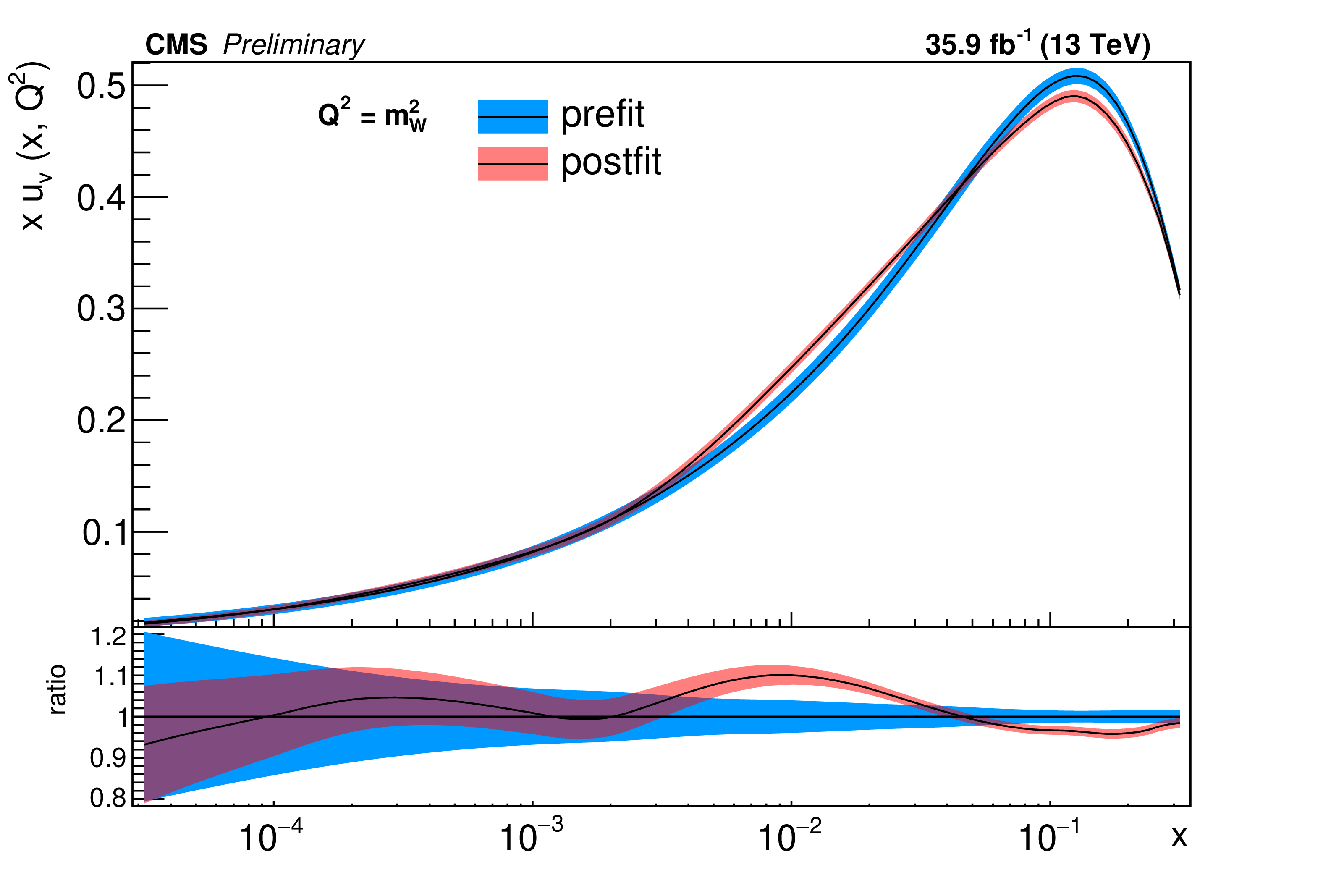
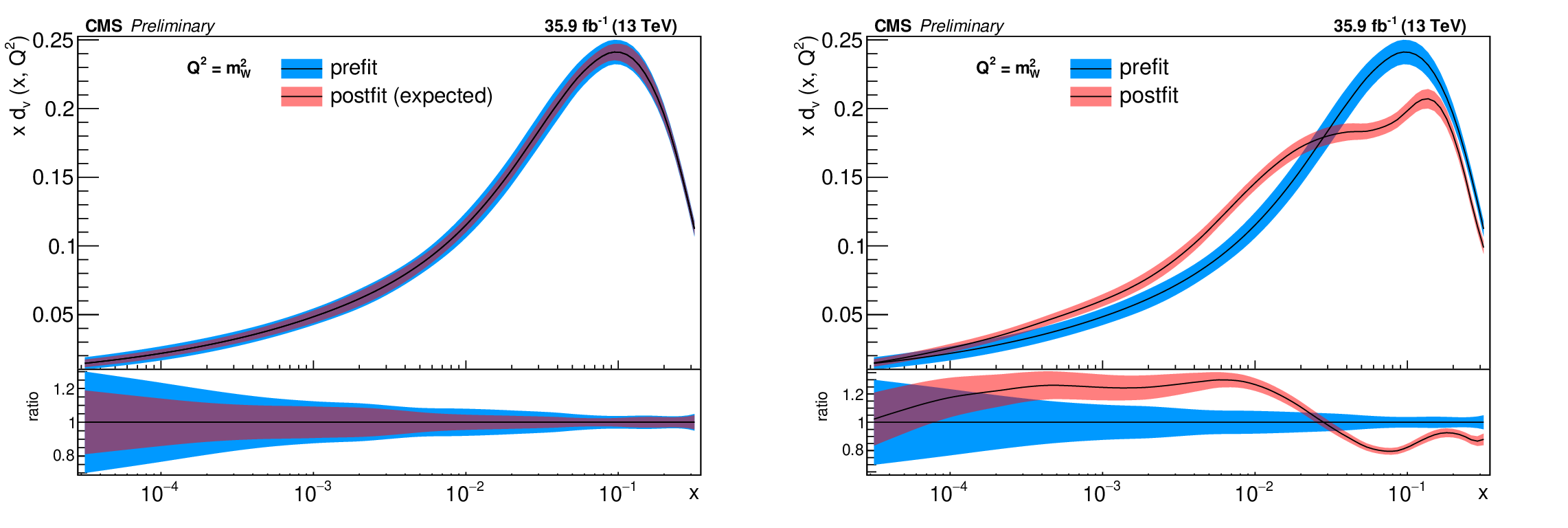
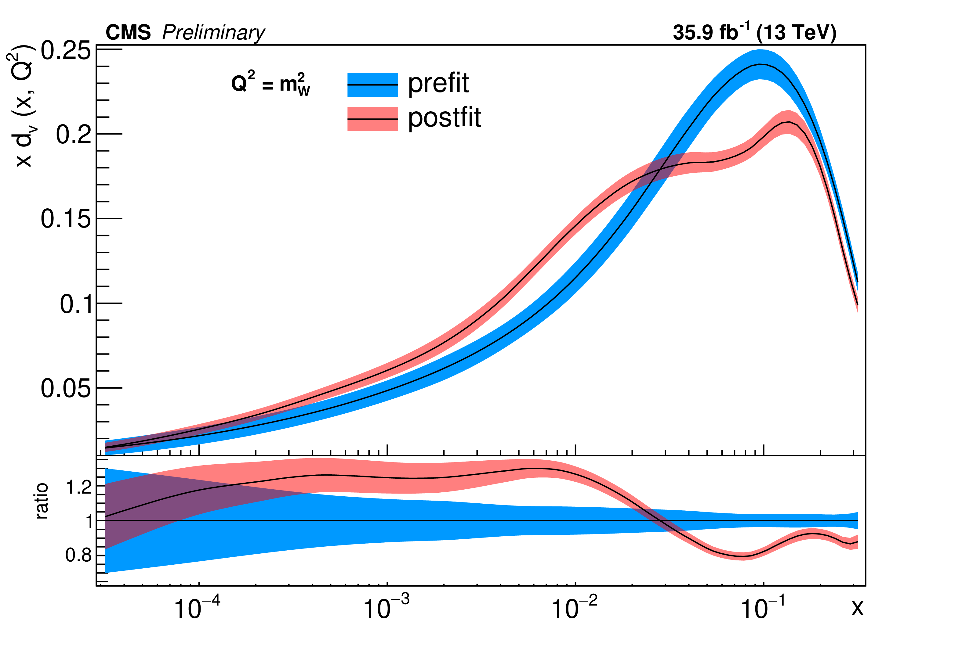
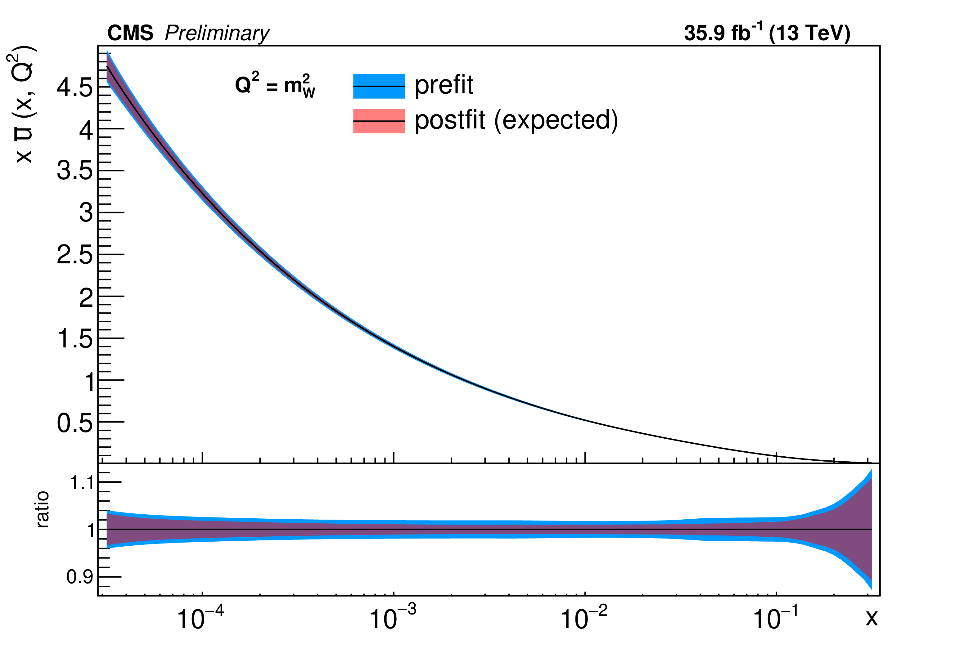
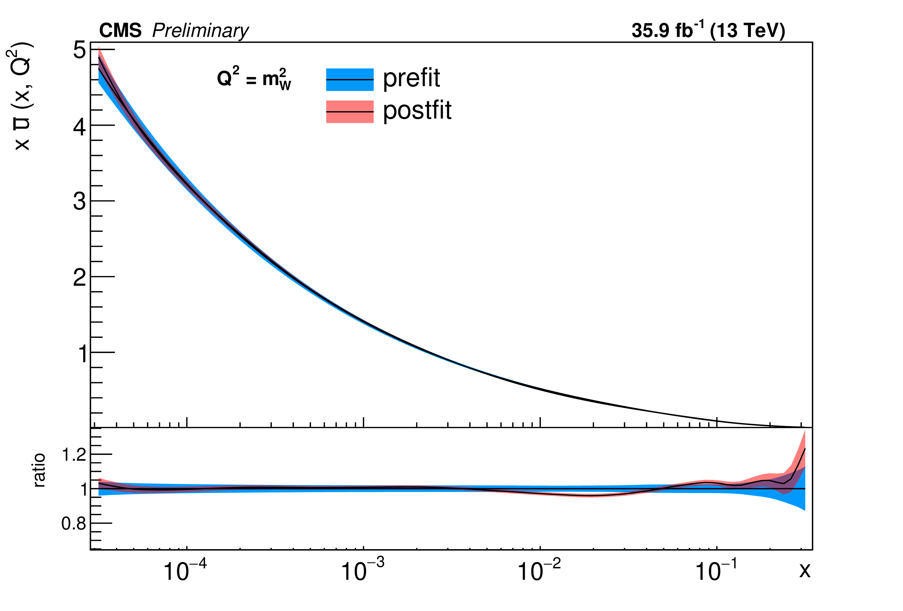
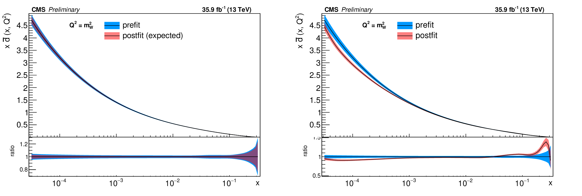
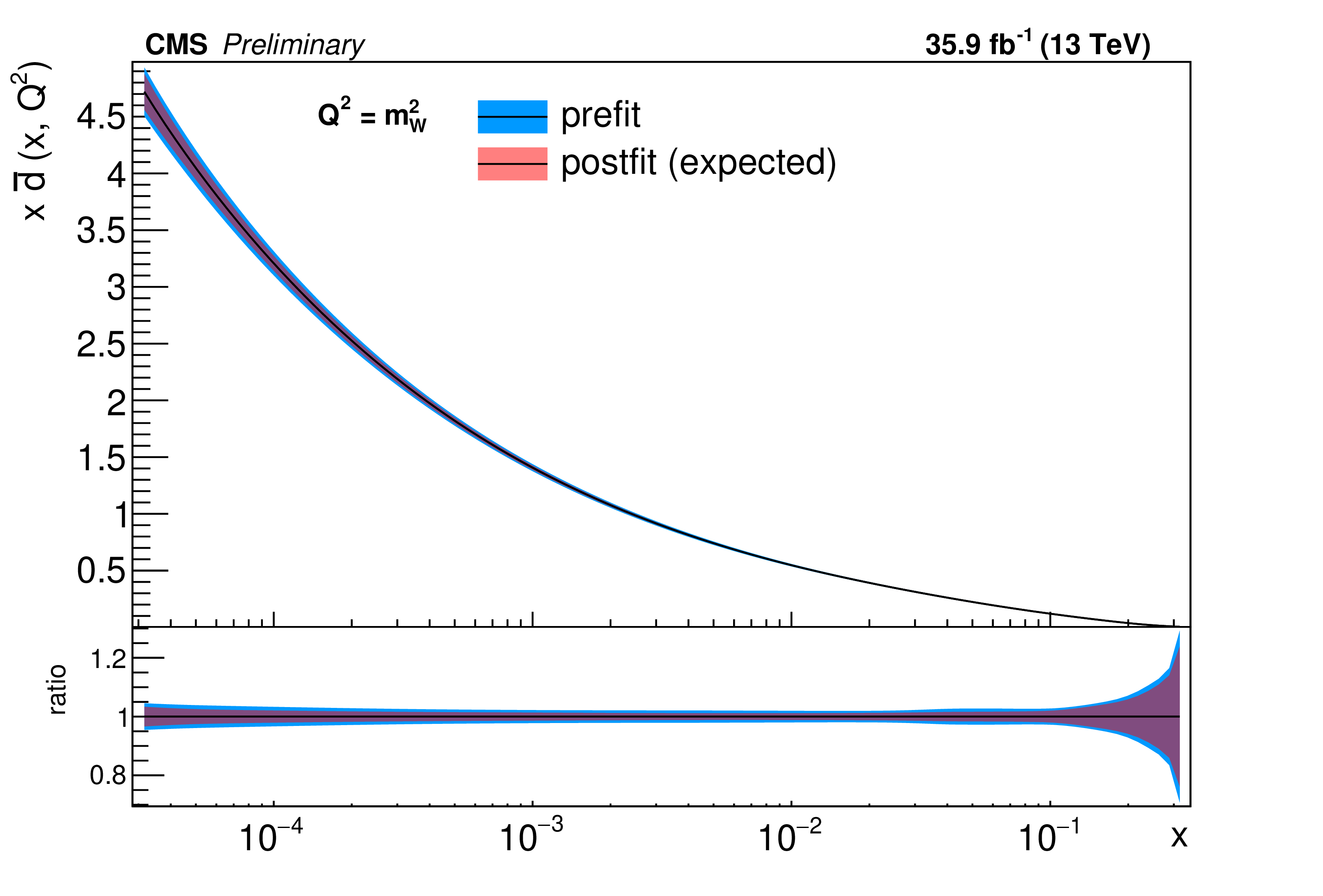
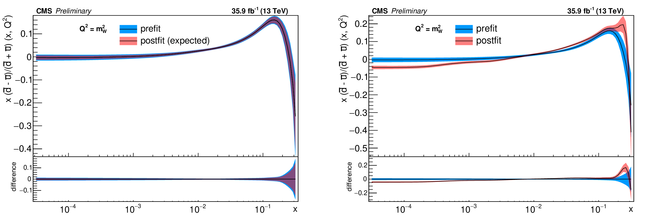
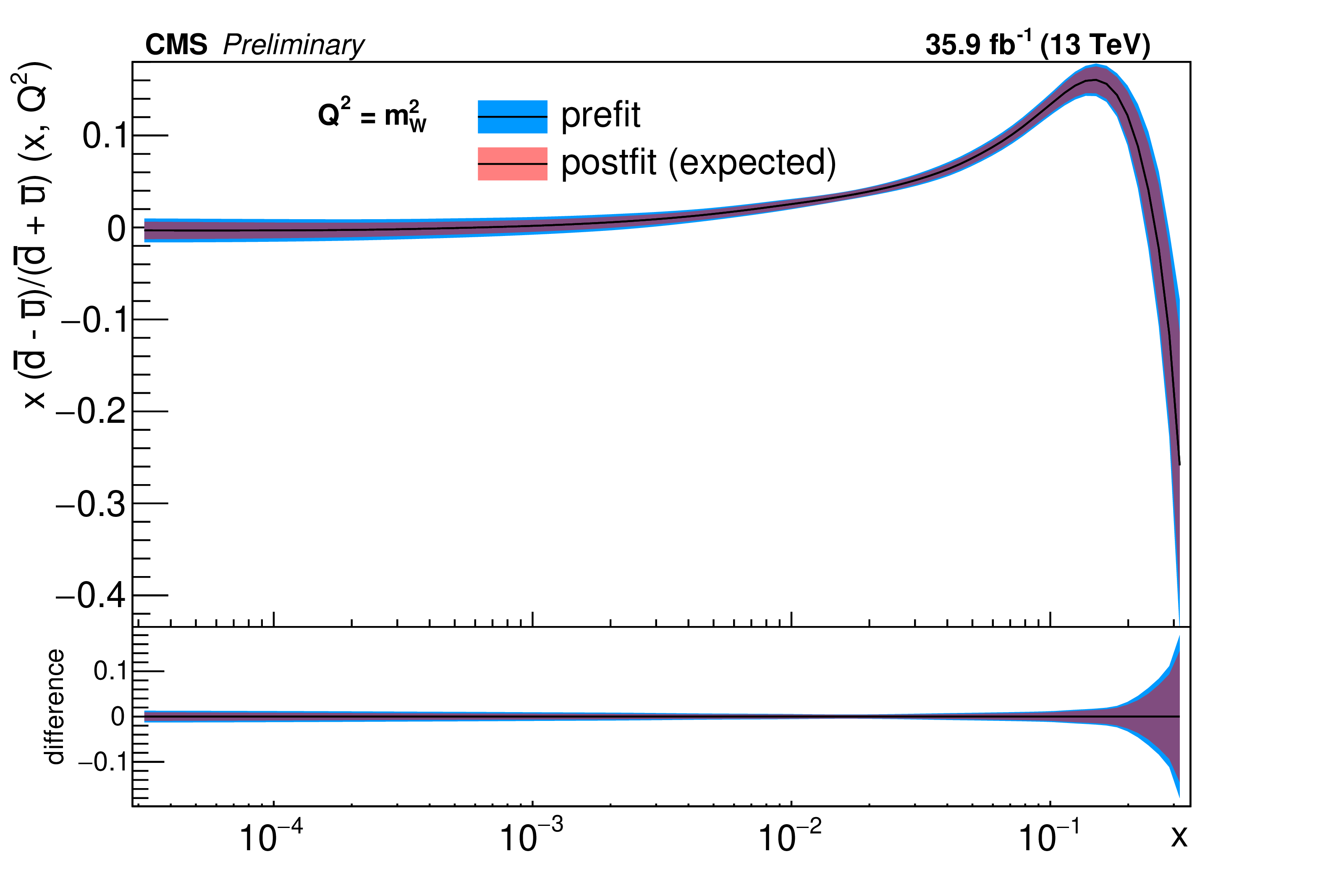
Additional Figure 2:
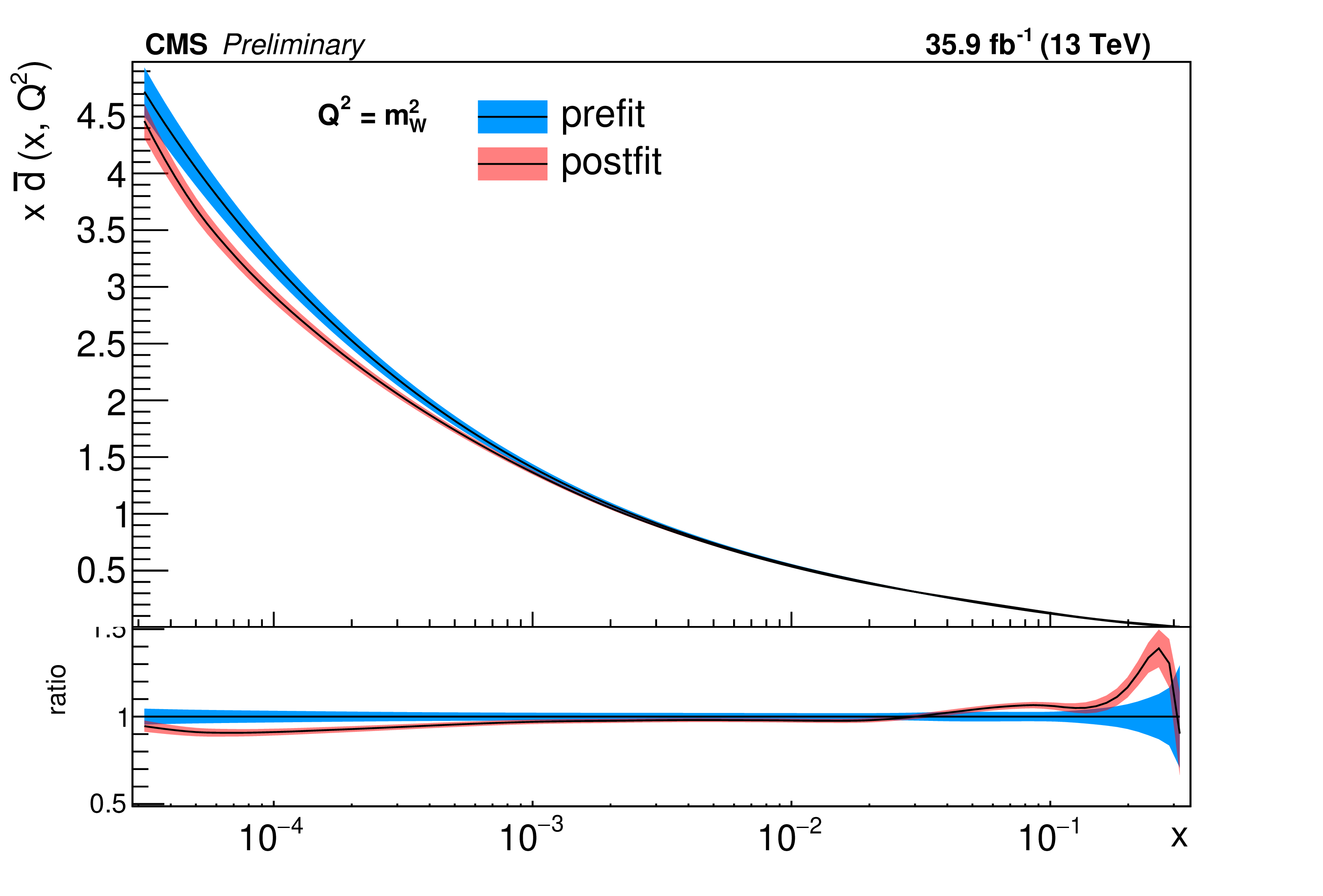
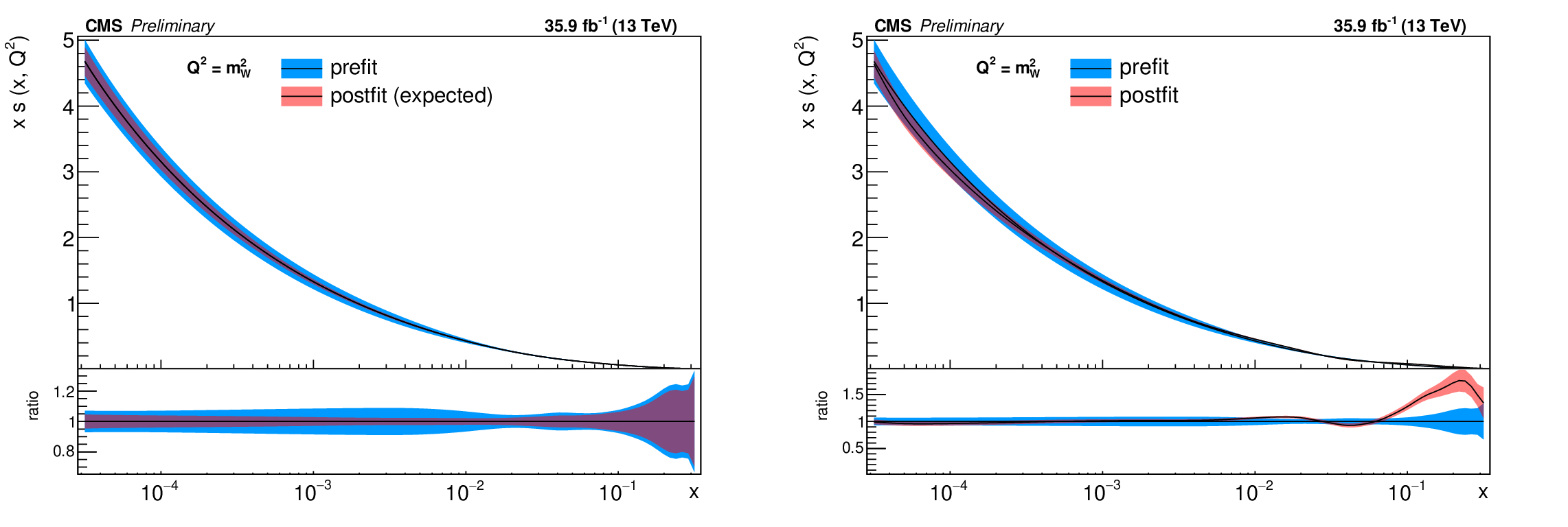
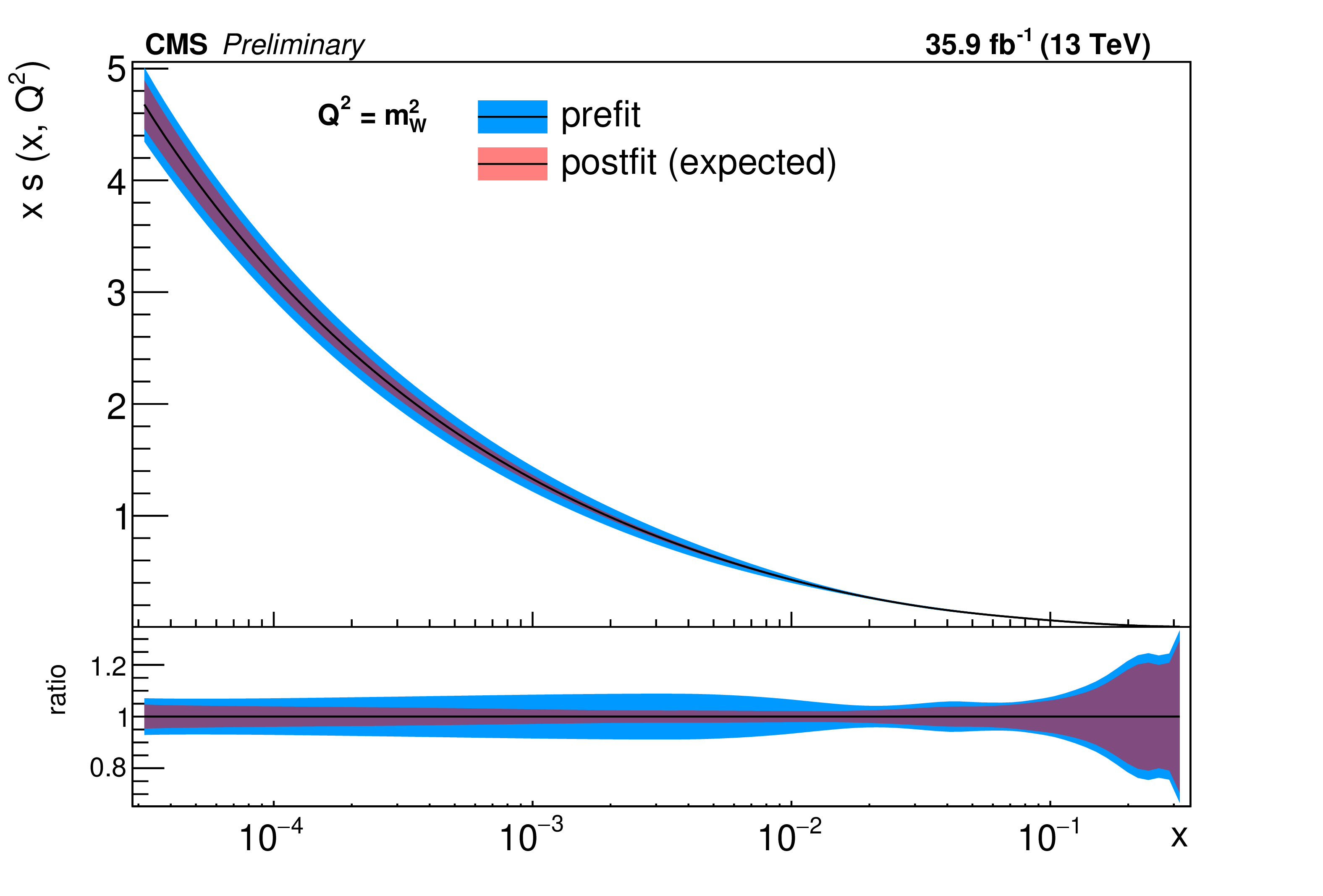
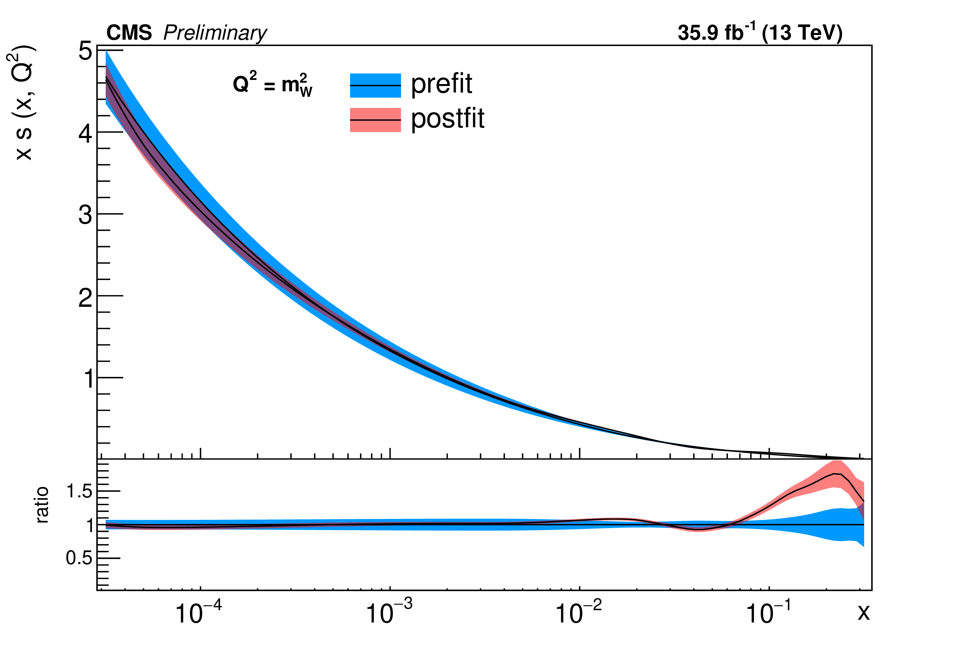
The post-fit nuisance parameter values and covariance matrix for the PDF and alphaS uncertainties from the fixed-parameter-of-interest fit described in Section 8.2 are propagated to the corresponding change in central value and uncertainty with respect to the input NNPDF3.0 NLO PDF set as a function of $x$ for fixed $Q^2=M_{\mathrm{W}}^2$. The profiling procedure employed here has the caveat that the results cannot be interpreted as a rigorous PDF determination in case the results are far from the input PDF, and that the measurement under consideration tends to have a larger weight than if it were included in a global PDF determination. Nevertheless the profiling procedure is useful to assess the sensitivity of the different parton distributions to this measurement, and its compatibility with the predictions of the input PDF set. Particular to this result is the fact that constraints are derived only at NLO + parton shower accuracy in QCD, and that there are possible limitations of the PDF set used with respect to newer sets. The presence of oscillatory behaviour in the valence quark distributions is in part related to anti-correlations between different $x$ values arising from the statistical uncertainties in the underlying measurement. |
png pdf |
Additional Figure 2-a:
The post-fit nuisance parameter values and covariance matrix for the PDF and alphaS uncertainties from the fixed-parameter-of-interest fit described in Section 8.2 are propagated to the corresponding change in central value and uncertainty with respect to the input NNPDF3.0 NLO PDF set as a function of $x$ for fixed $Q^2=M_{\mathrm{W}}^2$. The profiling procedure employed here has the caveat that the results cannot be interpreted as a rigorous PDF determination in case the results are far from the input PDF, and that the measurement under consideration tends to have a larger weight than if it were included in a global PDF determination. Nevertheless the profiling procedure is useful to assess the sensitivity of the different parton distributions to this measurement, and its compatibility with the predictions of the input PDF set. Particular to this result is the fact that constraints are derived only at NLO + parton shower accuracy in QCD, and that there are possible limitations of the PDF set used with respect to newer sets. The presence of oscillatory behaviour in the valence quark distributions is in part related to anti-correlations between different $x$ values arising from the statistical uncertainties in the underlying measurement. |
png pdf |
Additional Figure 2-b:
The post-fit nuisance parameter values and covariance matrix for the PDF and alphaS uncertainties from the fixed-parameter-of-interest fit described in Section 8.2 are propagated to the corresponding change in central value and uncertainty with respect to the input NNPDF3.0 NLO PDF set as a function of $x$ for fixed $Q^2=M_{\mathrm{W}}^2$. The profiling procedure employed here has the caveat that the results cannot be interpreted as a rigorous PDF determination in case the results are far from the input PDF, and that the measurement under consideration tends to have a larger weight than if it were included in a global PDF determination. Nevertheless the profiling procedure is useful to assess the sensitivity of the different parton distributions to this measurement, and its compatibility with the predictions of the input PDF set. Particular to this result is the fact that constraints are derived only at NLO + parton shower accuracy in QCD, and that there are possible limitations of the PDF set used with respect to newer sets. The presence of oscillatory behaviour in the valence quark distributions is in part related to anti-correlations between different $x$ values arising from the statistical uncertainties in the underlying measurement. |
png pdf |
Additional Figure 3:
The post-fit nuisance parameter values and covariance matrix for the PDF and alphaS uncertainties from the fixed-parameter-of-interest fit described in Section 8.2 are propagated to the corresponding change in central value and uncertainty with respect to the input NNPDF3.0 NLO PDF set as a function of $x$ for fixed $Q^2=M_{\mathrm{W}}^2$. The profiling procedure employed here has the caveat that the results cannot be interpreted as a rigorous PDF determination in case the results are far from the input PDF, and that the measurement under consideration tends to have a larger weight than if it were included in a global PDF determination. Nevertheless the profiling procedure is useful to assess the sensitivity of the different parton distributions to this measurement, and its compatibility with the predictions of the input PDF set. Particular to this result is the fact that constraints are derived only at NLO + parton shower accuracy in QCD, and that there are possible limitations of the PDF set used with respect to newer sets. The presence of oscillatory behaviour in the valence quark distributions is in part related to anti-correlations between different $x$ values arising from the statistical uncertainties in the underlying measurement. |

png pdf |
Additional Figure 3-a:
The post-fit nuisance parameter values and covariance matrix for the PDF and alphaS uncertainties from the fixed-parameter-of-interest fit described in Section 8.2 are propagated to the corresponding change in central value and uncertainty with respect to the input NNPDF3.0 NLO PDF set as a function of $x$ for fixed $Q^2=M_{\mathrm{W}}^2$. The profiling procedure employed here has the caveat that the results cannot be interpreted as a rigorous PDF determination in case the results are far from the input PDF, and that the measurement under consideration tends to have a larger weight than if it were included in a global PDF determination. Nevertheless the profiling procedure is useful to assess the sensitivity of the different parton distributions to this measurement, and its compatibility with the predictions of the input PDF set. Particular to this result is the fact that constraints are derived only at NLO + parton shower accuracy in QCD, and that there are possible limitations of the PDF set used with respect to newer sets. The presence of oscillatory behaviour in the valence quark distributions is in part related to anti-correlations between different $x$ values arising from the statistical uncertainties in the underlying measurement. |
png pdf |
Additional Figure 3-b:
The post-fit nuisance parameter values and covariance matrix for the PDF and alphaS uncertainties from the fixed-parameter-of-interest fit described in Section 8.2 are propagated to the corresponding change in central value and uncertainty with respect to the input NNPDF3.0 NLO PDF set as a function of $x$ for fixed $Q^2=M_{\mathrm{W}}^2$. The profiling procedure employed here has the caveat that the results cannot be interpreted as a rigorous PDF determination in case the results are far from the input PDF, and that the measurement under consideration tends to have a larger weight than if it were included in a global PDF determination. Nevertheless the profiling procedure is useful to assess the sensitivity of the different parton distributions to this measurement, and its compatibility with the predictions of the input PDF set. Particular to this result is the fact that constraints are derived only at NLO + parton shower accuracy in QCD, and that there are possible limitations of the PDF set used with respect to newer sets. The presence of oscillatory behaviour in the valence quark distributions is in part related to anti-correlations between different $x$ values arising from the statistical uncertainties in the underlying measurement. |

png pdf |
Additional Figure 4:
The post-fit nuisance parameter values and covariance matrix for the PDF and alphaS uncertainties from the fixed-parameter-of-interest fit described in Section 8.2 are propagated to the corresponding change in central value and uncertainty with respect to the input NNPDF3.0 NLO PDF set as a function of $x$ for fixed $Q^2=M_{\mathrm{W}}^2$. The profiling procedure employed here has the caveat that the results cannot be interpreted as a rigorous PDF determination in case the results are far from the input PDF, and that the measurement under consideration tends to have a larger weight than if it were included in a global PDF determination. Nevertheless the profiling procedure is useful to assess the sensitivity of the different parton distributions to this measurement, and its compatibility with the predictions of the input PDF set. Particular to this result is the fact that constraints are derived only at NLO + parton shower accuracy in QCD, and that there are possible limitations of the PDF set used with respect to newer sets. The presence of oscillatory behaviour in the valence quark distributions is in part related to anti-correlations between different $x$ values arising from the statistical uncertainties in the underlying measurement. |
png pdf |
Additional Figure 4-a:
The post-fit nuisance parameter values and covariance matrix for the PDF and alphaS uncertainties from the fixed-parameter-of-interest fit described in Section 8.2 are propagated to the corresponding change in central value and uncertainty with respect to the input NNPDF3.0 NLO PDF set as a function of $x$ for fixed $Q^2=M_{\mathrm{W}}^2$. The profiling procedure employed here has the caveat that the results cannot be interpreted as a rigorous PDF determination in case the results are far from the input PDF, and that the measurement under consideration tends to have a larger weight than if it were included in a global PDF determination. Nevertheless the profiling procedure is useful to assess the sensitivity of the different parton distributions to this measurement, and its compatibility with the predictions of the input PDF set. Particular to this result is the fact that constraints are derived only at NLO + parton shower accuracy in QCD, and that there are possible limitations of the PDF set used with respect to newer sets. The presence of oscillatory behaviour in the valence quark distributions is in part related to anti-correlations between different $x$ values arising from the statistical uncertainties in the underlying measurement. |
png pdf |
Additional Figure 4-b:
The post-fit nuisance parameter values and covariance matrix for the PDF and alphaS uncertainties from the fixed-parameter-of-interest fit described in Section 8.2 are propagated to the corresponding change in central value and uncertainty with respect to the input NNPDF3.0 NLO PDF set as a function of $x$ for fixed $Q^2=M_{\mathrm{W}}^2$. The profiling procedure employed here has the caveat that the results cannot be interpreted as a rigorous PDF determination in case the results are far from the input PDF, and that the measurement under consideration tends to have a larger weight than if it were included in a global PDF determination. Nevertheless the profiling procedure is useful to assess the sensitivity of the different parton distributions to this measurement, and its compatibility with the predictions of the input PDF set. Particular to this result is the fact that constraints are derived only at NLO + parton shower accuracy in QCD, and that there are possible limitations of the PDF set used with respect to newer sets. The presence of oscillatory behaviour in the valence quark distributions is in part related to anti-correlations between different $x$ values arising from the statistical uncertainties in the underlying measurement. |
png pdf |
Additional Figure 5:
The post-fit nuisance parameter values and covariance matrix for the PDF and alphaS uncertainties from the fixed-parameter-of-interest fit described in Section 8.2 are propagated to the corresponding change in central value and uncertainty with respect to the input NNPDF3.0 NLO PDF set as a function of $x$ for fixed $Q^2=M_{\mathrm{W}}^2$. The profiling procedure employed here has the caveat that the results cannot be interpreted as a rigorous PDF determination in case the results are far from the input PDF, and that the measurement under consideration tends to have a larger weight than if it were included in a global PDF determination. Nevertheless the profiling procedure is useful to assess the sensitivity of the different parton distributions to this measurement, and its compatibility with the predictions of the input PDF set. Particular to this result is the fact that constraints are derived only at NLO + parton shower accuracy in QCD, and that there are possible limitations of the PDF set used with respect to newer sets. The presence of oscillatory behaviour in the valence quark distributions is in part related to anti-correlations between different $x$ values arising from the statistical uncertainties in the underlying measurement. |
png pdf |
Additional Figure 5-a:
The post-fit nuisance parameter values and covariance matrix for the PDF and alphaS uncertainties from the fixed-parameter-of-interest fit described in Section 8.2 are propagated to the corresponding change in central value and uncertainty with respect to the input NNPDF3.0 NLO PDF set as a function of $x$ for fixed $Q^2=M_{\mathrm{W}}^2$. The profiling procedure employed here has the caveat that the results cannot be interpreted as a rigorous PDF determination in case the results are far from the input PDF, and that the measurement under consideration tends to have a larger weight than if it were included in a global PDF determination. Nevertheless the profiling procedure is useful to assess the sensitivity of the different parton distributions to this measurement, and its compatibility with the predictions of the input PDF set. Particular to this result is the fact that constraints are derived only at NLO + parton shower accuracy in QCD, and that there are possible limitations of the PDF set used with respect to newer sets. The presence of oscillatory behaviour in the valence quark distributions is in part related to anti-correlations between different $x$ values arising from the statistical uncertainties in the underlying measurement. |
png pdf |
Additional Figure 5-b:
The post-fit nuisance parameter values and covariance matrix for the PDF and alphaS uncertainties from the fixed-parameter-of-interest fit described in Section 8.2 are propagated to the corresponding change in central value and uncertainty with respect to the input NNPDF3.0 NLO PDF set as a function of $x$ for fixed $Q^2=M_{\mathrm{W}}^2$. The profiling procedure employed here has the caveat that the results cannot be interpreted as a rigorous PDF determination in case the results are far from the input PDF, and that the measurement under consideration tends to have a larger weight than if it were included in a global PDF determination. Nevertheless the profiling procedure is useful to assess the sensitivity of the different parton distributions to this measurement, and its compatibility with the predictions of the input PDF set. Particular to this result is the fact that constraints are derived only at NLO + parton shower accuracy in QCD, and that there are possible limitations of the PDF set used with respect to newer sets. The presence of oscillatory behaviour in the valence quark distributions is in part related to anti-correlations between different $x$ values arising from the statistical uncertainties in the underlying measurement. |
png pdf |
Additional Figure 6:
The post-fit nuisance parameter values and covariance matrix for the PDF and alphaS uncertainties from the fixed-parameter-of-interest fit described in Section 8.2 are propagated to the corresponding change in central value and uncertainty with respect to the input NNPDF3.0 NLO PDF set as a function of $x$ for fixed $Q^2=M_{\mathrm{W}}^2$. The profiling procedure employed here has the caveat that the results cannot be interpreted as a rigorous PDF determination in case the results are far from the input PDF, and that the measurement under consideration tends to have a larger weight than if it were included in a global PDF determination. Nevertheless the profiling procedure is useful to assess the sensitivity of the different parton distributions to this measurement, and its compatibility with the predictions of the input PDF set. Particular to this result is the fact that constraints are derived only at NLO + parton shower accuracy in QCD, and that there are possible limitations of the PDF set used with respect to newer sets. The presence of oscillatory behaviour in the valence quark distributions is in part related to anti-correlations between different $x$ values arising from the statistical uncertainties in the underlying measurement. |
png pdf |
Additional Figure 6-a:
The post-fit nuisance parameter values and covariance matrix for the PDF and alphaS uncertainties from the fixed-parameter-of-interest fit described in Section 8.2 are propagated to the corresponding change in central value and uncertainty with respect to the input NNPDF3.0 NLO PDF set as a function of $x$ for fixed $Q^2=M_{\mathrm{W}}^2$. The profiling procedure employed here has the caveat that the results cannot be interpreted as a rigorous PDF determination in case the results are far from the input PDF, and that the measurement under consideration tends to have a larger weight than if it were included in a global PDF determination. Nevertheless the profiling procedure is useful to assess the sensitivity of the different parton distributions to this measurement, and its compatibility with the predictions of the input PDF set. Particular to this result is the fact that constraints are derived only at NLO + parton shower accuracy in QCD, and that there are possible limitations of the PDF set used with respect to newer sets. The presence of oscillatory behaviour in the valence quark distributions is in part related to anti-correlations between different $x$ values arising from the statistical uncertainties in the underlying measurement. |
png pdf |
Additional Figure 6-b:
The post-fit nuisance parameter values and covariance matrix for the PDF and alphaS uncertainties from the fixed-parameter-of-interest fit described in Section 8.2 are propagated to the corresponding change in central value and uncertainty with respect to the input NNPDF3.0 NLO PDF set as a function of $x$ for fixed $Q^2=M_{\mathrm{W}}^2$. The profiling procedure employed here has the caveat that the results cannot be interpreted as a rigorous PDF determination in case the results are far from the input PDF, and that the measurement under consideration tends to have a larger weight than if it were included in a global PDF determination. Nevertheless the profiling procedure is useful to assess the sensitivity of the different parton distributions to this measurement, and its compatibility with the predictions of the input PDF set. Particular to this result is the fact that constraints are derived only at NLO + parton shower accuracy in QCD, and that there are possible limitations of the PDF set used with respect to newer sets. The presence of oscillatory behaviour in the valence quark distributions is in part related to anti-correlations between different $x$ values arising from the statistical uncertainties in the underlying measurement. |

png pdf |
Additional Figure 7:
The post-fit nuisance parameter values and covariance matrix for the PDF and alphaS uncertainties from the fixed-parameter-of-interest fit described in Section 8.2 are propagated to the corresponding change in central value and uncertainty with respect to the input NNPDF3.0 NLO PDF set as a function of $x$ for fixed $Q^2=M_{\mathrm{W}}^2$. The profiling procedure employed here has the caveat that the results cannot be interpreted as a rigorous PDF determination in case the results are far from the input PDF, and that the measurement under consideration tends to have a larger weight than if it were included in a global PDF determination. Nevertheless the profiling procedure is useful to assess the sensitivity of the different parton distributions to this measurement, and its compatibility with the predictions of the input PDF set. Particular to this result is the fact that constraints are derived only at NLO + parton shower accuracy in QCD, and that there are possible limitations of the PDF set used with respect to newer sets. The presence of oscillatory behaviour in the valence quark distributions is in part related to anti-correlations between different $x$ values arising from the statistical uncertainties in the underlying measurement. |

png pdf |
Additional Figure 7-a:
The post-fit nuisance parameter values and covariance matrix for the PDF and alphaS uncertainties from the fixed-parameter-of-interest fit described in Section 8.2 are propagated to the corresponding change in central value and uncertainty with respect to the input NNPDF3.0 NLO PDF set as a function of $x$ for fixed $Q^2=M_{\mathrm{W}}^2$. The profiling procedure employed here has the caveat that the results cannot be interpreted as a rigorous PDF determination in case the results are far from the input PDF, and that the measurement under consideration tends to have a larger weight than if it were included in a global PDF determination. Nevertheless the profiling procedure is useful to assess the sensitivity of the different parton distributions to this measurement, and its compatibility with the predictions of the input PDF set. Particular to this result is the fact that constraints are derived only at NLO + parton shower accuracy in QCD, and that there are possible limitations of the PDF set used with respect to newer sets. The presence of oscillatory behaviour in the valence quark distributions is in part related to anti-correlations between different $x$ values arising from the statistical uncertainties in the underlying measurement. |

png pdf |
Additional Figure 7-b:
The post-fit nuisance parameter values and covariance matrix for the PDF and alphaS uncertainties from the fixed-parameter-of-interest fit described in Section 8.2 are propagated to the corresponding change in central value and uncertainty with respect to the input NNPDF3.0 NLO PDF set as a function of $x$ for fixed $Q^2=M_{\mathrm{W}}^2$. The profiling procedure employed here has the caveat that the results cannot be interpreted as a rigorous PDF determination in case the results are far from the input PDF, and that the measurement under consideration tends to have a larger weight than if it were included in a global PDF determination. Nevertheless the profiling procedure is useful to assess the sensitivity of the different parton distributions to this measurement, and its compatibility with the predictions of the input PDF set. Particular to this result is the fact that constraints are derived only at NLO + parton shower accuracy in QCD, and that there are possible limitations of the PDF set used with respect to newer sets. The presence of oscillatory behaviour in the valence quark distributions is in part related to anti-correlations between different $x$ values arising from the statistical uncertainties in the underlying measurement. |
png pdf |
Additional Figure 8:
The post-fit nuisance parameter values and covariance matrix for the PDF and alphaS uncertainties from the fixed-parameter-of-interest fit described in Section 8.2 are propagated to the corresponding change in central value and uncertainty with respect to the input NNPDF3.0 NLO PDF set as a function of $x$ for fixed $Q^2=M_{\mathrm{W}}^2$. The profiling procedure employed here has the caveat that the results cannot be interpreted as a rigorous PDF determination in case the results are far from the input PDF, and that the measurement under consideration tends to have a larger weight than if it were included in a global PDF determination. Nevertheless the profiling procedure is useful to assess the sensitivity of the different parton distributions to this measurement, and its compatibility with the predictions of the input PDF set. Particular to this result is the fact that constraints are derived only at NLO + parton shower accuracy in QCD, and that there are possible limitations of the PDF set used with respect to newer sets. The presence of oscillatory behaviour in the valence quark distributions is in part related to anti-correlations between different $x$ values arising from the statistical uncertainties in the underlying measurement. |
png pdf |
Additional Figure 8-a:
The post-fit nuisance parameter values and covariance matrix for the PDF and alphaS uncertainties from the fixed-parameter-of-interest fit described in Section 8.2 are propagated to the corresponding change in central value and uncertainty with respect to the input NNPDF3.0 NLO PDF set as a function of $x$ for fixed $Q^2=M_{\mathrm{W}}^2$. The profiling procedure employed here has the caveat that the results cannot be interpreted as a rigorous PDF determination in case the results are far from the input PDF, and that the measurement under consideration tends to have a larger weight than if it were included in a global PDF determination. Nevertheless the profiling procedure is useful to assess the sensitivity of the different parton distributions to this measurement, and its compatibility with the predictions of the input PDF set. Particular to this result is the fact that constraints are derived only at NLO + parton shower accuracy in QCD, and that there are possible limitations of the PDF set used with respect to newer sets. The presence of oscillatory behaviour in the valence quark distributions is in part related to anti-correlations between different $x$ values arising from the statistical uncertainties in the underlying measurement. |
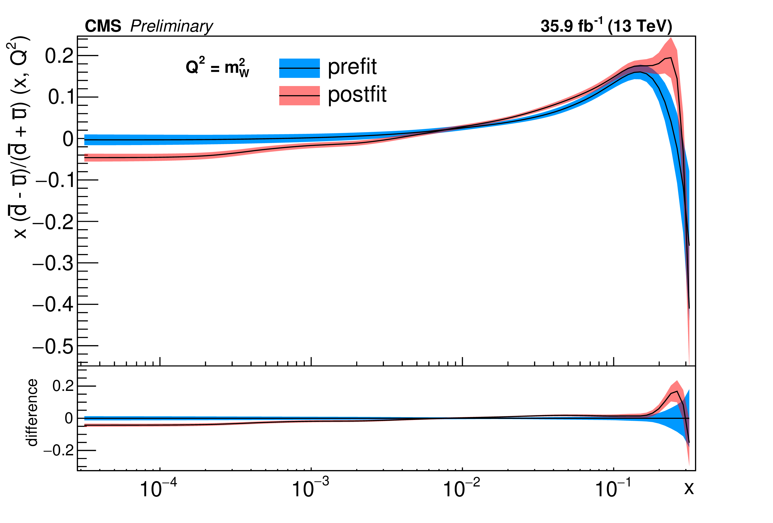
png pdf |
Additional Figure 8-b:
The post-fit nuisance parameter values and covariance matrix for the PDF and alphaS uncertainties from the fixed-parameter-of-interest fit described in Section 8.2 are propagated to the corresponding change in central value and uncertainty with respect to the input NNPDF3.0 NLO PDF set as a function of $x$ for fixed $Q^2=M_{\mathrm{W}}^2$. The profiling procedure employed here has the caveat that the results cannot be interpreted as a rigorous PDF determination in case the results are far from the input PDF, and that the measurement under consideration tends to have a larger weight than if it were included in a global PDF determination. Nevertheless the profiling procedure is useful to assess the sensitivity of the different parton distributions to this measurement, and its compatibility with the predictions of the input PDF set. Particular to this result is the fact that constraints are derived only at NLO + parton shower accuracy in QCD, and that there are possible limitations of the PDF set used with respect to newer sets. The presence of oscillatory behaviour in the valence quark distributions is in part related to anti-correlations between different $x$ values arising from the statistical uncertainties in the underlying measurement. |
| References | ||||
| 1 | S. L. Glashow | Partial symmetries of weak interactions | NP 22 (1961) 579 | |
| 2 | S. Weinberg | A model of leptons | PRL 19 (1967) 1264 | |
| 3 | A. Salam and J. C. Ward | Electromagnetic and weak interactions | PL13 (1964) 168 | |
| 4 | J. D. Bjorken and E. A. Paschos | Inelastic electron-proton and $ {\gamma} $-proton scattering and the structure of the nucleon | PR185 (1969) 1975 | |
| 5 | W. J. Stirling and A. D. Martin | Parton distribution uncertainty in the measurement of M$ _\mathrm{W} $ in proton - anti-proton collisions | PLB 237 (1990) 551 | |
| 6 | ATLAS Collaboration | Measurement of the W-boson mass in pp collisions at $ \sqrt{s}= $ 7 TeV with the ATLAS detector | EPJC 78 (2018) 110 | 1701.07240 |
| 7 | CMS Collaboration | Measurement of the differential Drell-Yan cross section in proton-proton collisions at $ \sqrt{\mathrm{s}} = $ 13 TeV | JHEP 12 (2019) 059 | CMS-SMP-17-001 1812.10529 |
| 8 | CMS Collaboration | Measurement of the weak mixing angle using the forward-backward asymmetry of Drell-Yan events in pp collisions at 8 TeV | EPJC 78 (2018) 701 | |
| 9 | ATLAS Collaboration | Measurement of the Drell-Yan triple-differential cross section in pp collisions at $ \sqrt{s} = $ 8 TeV | JHEP 12 (2017) 059 | 1710.05167 |
| 10 | CDF Collaboration | Direct measurement of the W production charge asymmetry in $ \mathrm{p}\bar{\mathrm{p}} $ collisions at $ \sqrt{s} = $ 1.96 TeV | PRL 102 (2009) 181801 | 0901.2169 |
| 11 | D0 Collaboration | Measurement of the muon charge asymmetry in $ \mathrm{p}\bar{\mathrm{p}} \to $ W+X $ \to \mu \nu $ + X events at $ \sqrt{s} = $ 1.96 TeV | PRD 88 (2013) 091102 | 1309.2591 |
| 12 | ATLAS Collaboration | Precision measurement and interpretation of inclusive W$ ^+ $ , W$ ^- $ and $ \mathrm{Z}/\gamma ^* $ production cross sections with the ATLAS detector | EPJC 77 (2017) 367 | 1612.03016 |
| 13 | ATLAS Collaboration | Measurement of the cross-section and charge asymmetry of W bosons produced in proton-proton collisions at $ \sqrt{s}= $ 8 TeV with the ATLAS detector | EPJC 79 (2019) 760 | 1904.05631 |
| 14 | CMS Collaboration | Measurement of the electron charge asymmetry in inclusive W production in pp collisions at $ \sqrt{s}= $ 7 TeV | PRL 109 (2012) 111806 | CMS-SMP-12-001 1206.2598 |
| 15 | CMS Collaboration | Measurement of the muon charge asymmetry in inclusive pp $ \to $ W+X production at $ \sqrt s = $ 7 TeV and an improved determination of light parton distribution functions | PRD 90 (2014) 032004 | CMS-SMP-12-021 1312.6283 |
| 16 | CMS Collaboration | Measurement of the differential cross section and charge asymmetry for inclusive $ \mathrm {p}\mathrm {p}\rightarrow \mathrm {W}^{\pm}+\mathrm{X} $ production at $ {\sqrt{s}} = $ 8 TeV | EPJC 76 (2016) 469 | CMS-SMP-14-022 1603.01803 |
| 17 | LHCb Collaboration | Inclusive W and Z production in the forward region at $ \sqrt{s} = $ 7 TeV | JHEP 06 (2012) 058 | 1204.1620 |
| 18 | LHCb Collaboration | Measurement of forward W and Z boson production in pp collisions at $ \sqrt{s}= $ 8 TeV | JHEP 01 (2016) 155 | 1511.08039 |
| 19 | E. Manca, O. Cerri, N. Foppiani, and G. Rolandi | About the rapidity and helicity distributions of the W bosons produced at LHC | JHEP 12 (2017) 130 | 1707.09344 |
| 20 | CMS Collaboration | The CMS experiment at the CERN LHC | JINST 3 (2008) S08004 | CMS-00-001 |
| 21 | CMS Collaboration | The CMS trigger system | JINST 12 (2017) P01020 | CMS-TRG-12-001 1609.02366 |
| 22 | J. Alwall et al. | The automated computation of tree-level and next-to-leading order differential cross sections, and their matching to parton shower simulations | JHEP 07 (2014) 079 | 1405.0301 |
| 23 | S. Frixione, P. Nason, and C. Oleari | Matching NLO QCD computations with parton shower simulations: the POWHEG method | JHEP 11 (2007) 070 | 0709.2092 |
| 24 | T. Sjostrand et al. | An Introduction to PYTHIA 8.2 | CPC 191 (2015) 159 | 1410.3012 |
| 25 | P. Skands, S. Carrazza, and J. Rojo | Tuning PYTHIA 8.1: the Monash 2013 tune | EPJC 74 (2014) 3024 | 1404.5630 |
| 26 | NNPDF Collaboration | Parton distributions for the LHC Run II | JHEP 04 (2015) 040 | 1410.8849 |
| 27 | CMS Collaboration | Measurements of differential Z boson production cross sections in proton-proton collisions at $ \sqrt{s} = $ 13 TeV | JHEP 12 (2019) 061 | CMS-SMP-17-010 1909.04133 |
| 28 | GEANT4 Collaboration | GEANT4 - a simulation toolkit | NIMA 506 (2003) 250 | |
| 29 | CMS Collaboration | Particle-flow reconstruction and global event description with the CMS detector | JINST 12 (2017) P10003 | CMS-PRF-14-001 1706.04965 |
| 30 | CMS Collaboration | Energy calibration and resolution of the CMS electromagnetic calorimeter in pp collisions at $ \sqrt{s} = $ 7 TeV | JINST 8 (2013) P09009 | CMS-EGM-11-001 1306.2016 |
| 31 | CMS Collaboration | Performance of electron reconstruction and selection with the CMS detector in proton-proton collisions at $ \sqrt{s} = $ 8 TeV | JINST 10 (2015) P06005 | CMS-EGM-13-001 1502.02701 |
| 32 | CMS Collaboration | Electron and photon performance in CMS with the full 2017 data sample and additional 2016 highlights for the CALOR 2018 conference | CDS | |
| 33 | CMS Collaboration | Measurements of inclusive W and Z cross sections in pp collisions at $ \sqrt{s}= $ 7 TeV | JHEP 01 (2011) 080 | CMS-EWK-10-002 1012.2466 |
| 34 | J. Gaiser | Charmonium Spectroscopy From Radiative Decays of the $\mathrm{J}/\psi$ | PhD thesis, SLAC | |
| 35 | Z. Bern et al. | Left-handed W bosons at the LHC | PRD 84 (2011) 034008 | 1103.5445 |
| 36 | J. C. Collins and D. E. Soper | Angular distribution of dileptons in high-energy hadron collisions | PRD 16 (1977) 2219 | |
| 37 | R. K. Ellis, W. J. Stirling, and B. R. Webber | QCD and collider physics | Camb. Monogr. Part. Phys. NP Cosmol. 8 (1996)1 | |
| 38 | M. Abadi et al. | TensorFlow: Large-scale machine learning on heterogeneous systems | 2015 Software available from tensorflow.org. \url https://www.tensorflow.org/ | |
| 39 | The ATLAS Collaboration, The CMS Collaboration, The LHC Higgs Combination Group Collaboration | Procedure for the LHC Higgs boson search combination in summer 2011 | CMS-NOTE-2011-005 | |
| 40 | A. Bodek et al. | Extracting muon momentum scale corrections for hadron collider experiments | EPJC 72 (2012) 2194 | 1208.3710 |
| 41 | S. Carrazza et al. | An unbiased Hessian representation for Monte Carlo PDFs | EPJC 75 (2015) 369 | 1505.06736 |
| 42 | CMS Collaboration | Measurement of the lepton charge asymmetry in inclusive W production in pp collisions at $ \sqrt{s} = $ 7 TeV | JHEP 04 (2011) 050 | CMS-EWK-10-006 1103.3470 |
| 43 | CMS Collaboration | CMS luminosity measurements for the 2016 data taking period | CMS-PAS-LUM-17-001 | CMS-PAS-LUM-17-001 |
| 44 | P. Golonka and Z. Was | PHOTOS Monte Carlo: a precision tool for QED corrections in Z and W decays | EPJC 45 (2006) 97 | hep-ph/0506026 |
| 45 | R. J. Barlow and C. Beeston | Fitting using finite Monte Carlo samples | CPC 77 (1993) 219 | |
| 46 | NNPDF Collaboration | A first determination of parton distributions with theoretical uncertainties | EPJC 79 (2019) 838 | 1905.04311 |
| 47 | NNPDF Collaboration | Parton distributions with theory uncertainties: general formalism and first phenomenological studies | EPJC 79 (2019) 931 | 1906.10698 |
|
|
Compact Muon Solenoid LHC, CERN |
|

|

|

|

|

|