

Compact Muon Solenoid
LHC, CERN
| CMS-PAS-SMP-18-011 | ||
| A precision measurement of the W boson decay branching fractions in pp collisions at $\sqrt{s} = $ 13 TeV | ||
| CMS Collaboration | ||
| March 2021 | ||
| Abstract: The leptonic and inclusive hadronic decay branching fractions of the W boson are studied using 35.9 fb$^{-1}$ of proton-proton collision data collected at $\sqrt{s}= $ 13 TeV during the 2016 run of the CMS experiment. Events characterized by the production of two W boson, or of a W boson accompanied by jets, are selected. Multiple event categories sensitive to the signal processes are defined based on the presence of energetic isolated charged leptons, the number of hadronic jets, and the number of b-tagged jets. A maximum likelihood estimate of the W branching fractions is carried out by fitting to the data in each event category simultaneously. The branching fractions of the W boson decaying into electron, muon, and tau lepton final states amount to (10.83 $\pm$ 0.1 )%, (10.94 $\pm$ 0.08 )%, and (10.77 $\pm$ 0.21 )%, respectively, supporting the hypothesis of lepton universality for the weak interaction. Under the assumption of lepton universality, the inclusive leptonic and hadronic decay branching fractions are found to be (10.89 $\pm$ 0.08 )% and (67.32 $\pm$ 0.23 )%, respectively. From these results, three standard model quantities are subsequently derived: the sum square of elements in the first two rows of the Cabibbo-Kobayashi-Maskawa (CKM) matrix $\sum{|\mathrm{V_{ij}}|^{2}} = $ 1.989 $\pm$ 0.021, the CKM element $|\mathrm{V_{cs}}| = $ 0.969 $\pm$ 0.011, and the strong coupling constant at the W mass scale, $\alpha_\mathrm{S}(m_\mathrm{W}) = $ 0.094 $\pm$ 0.033. | ||
|
Links:
CDS record (PDF) ;
inSPIRE record ;
CADI line (restricted) ;
These preliminary results are superseded in this paper, Submitted to PRD. The superseded preliminary plots can be found here. |
||
| Figures & Tables | Summary | Additional Figures & Tables | References | CMS Publications |
|---|
| Figures | |
png pdf |
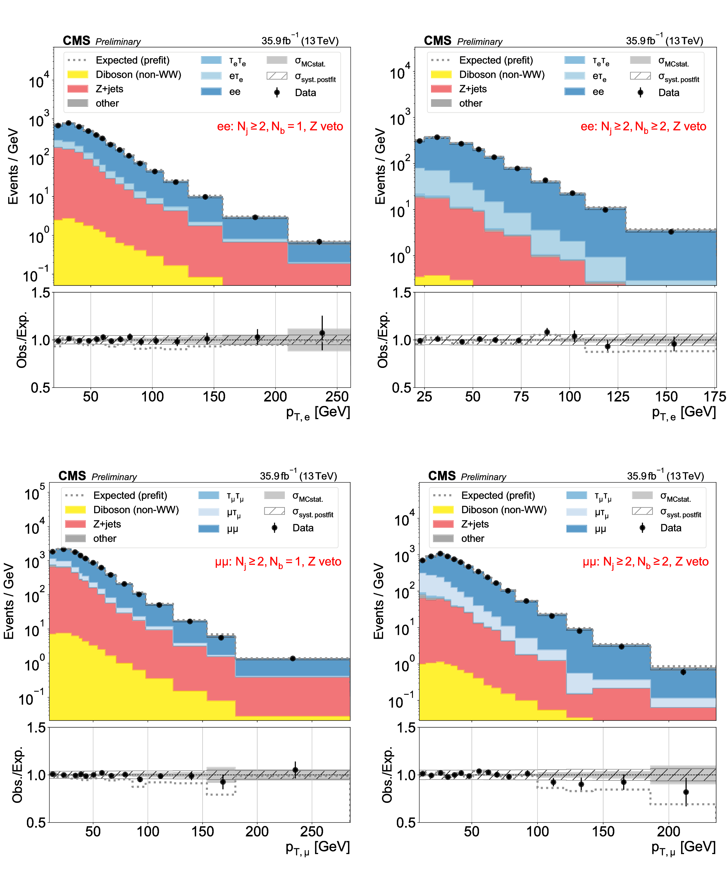
Figure 1:
Distributions used as inputs for the binned likelihood fits for the ee (upper) and $\mu \mu $ (lower) categories, with the requirement of one (left) or more than one (right) b-tagged jets. The bottom panels show the ratio of data over prefit (dotted line) and postfit (black circles) expectations, with associated statistical uncertainties (hatched area) and postfit systematic uncertainties (shaded gray). |

png pdf |
Figure 1-a:
Distributions used as inputs for the binned likelihood fits for the ee (upper) and $\mu \mu $ (lower) categories, with the requirement of one (left) or more than one (right) b-tagged jets. The bottom panels show the ratio of data over prefit (dotted line) and postfit (black circles) expectations, with associated statistical uncertainties (hatched area) and postfit systematic uncertainties (shaded gray). |
png pdf |
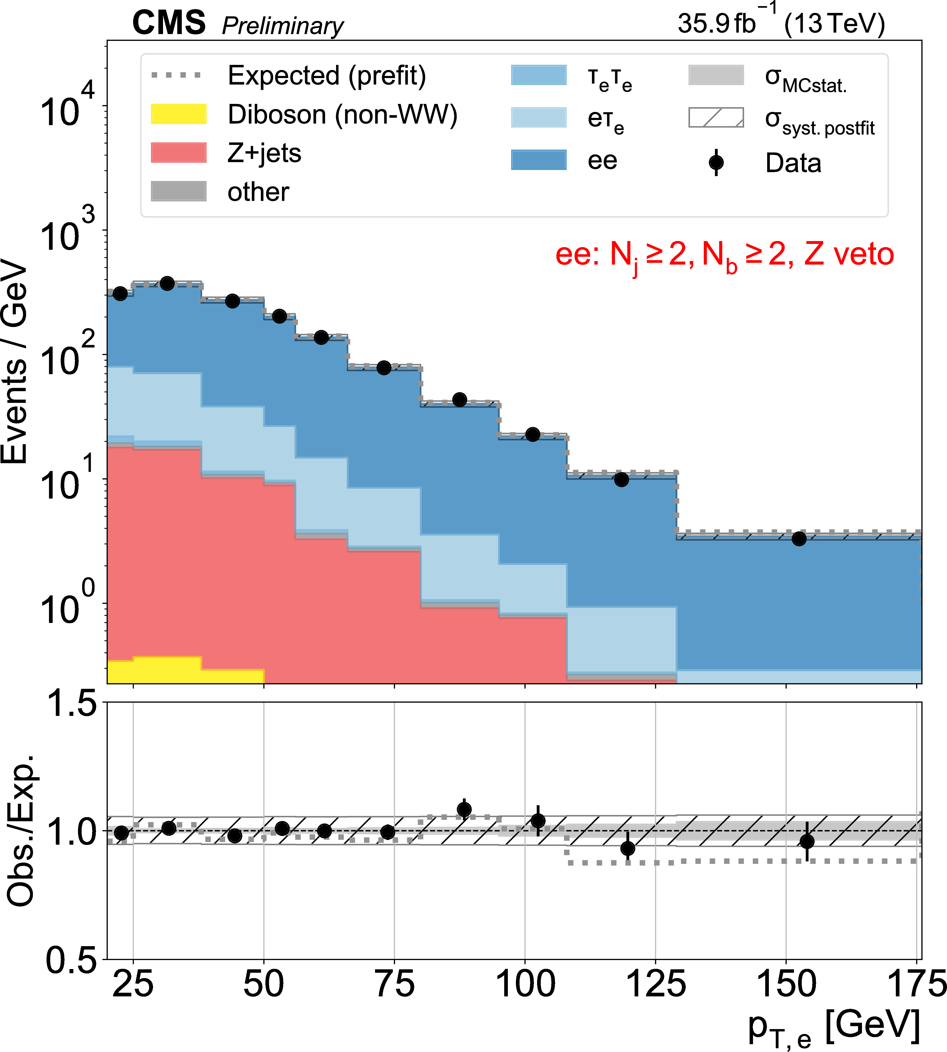
Figure 1-b:
Distributions used as inputs for the binned likelihood fits for the ee (upper) and $\mu \mu $ (lower) categories, with the requirement of one (left) or more than one (right) b-tagged jets. The bottom panels show the ratio of data over prefit (dotted line) and postfit (black circles) expectations, with associated statistical uncertainties (hatched area) and postfit systematic uncertainties (shaded gray). |
png pdf |
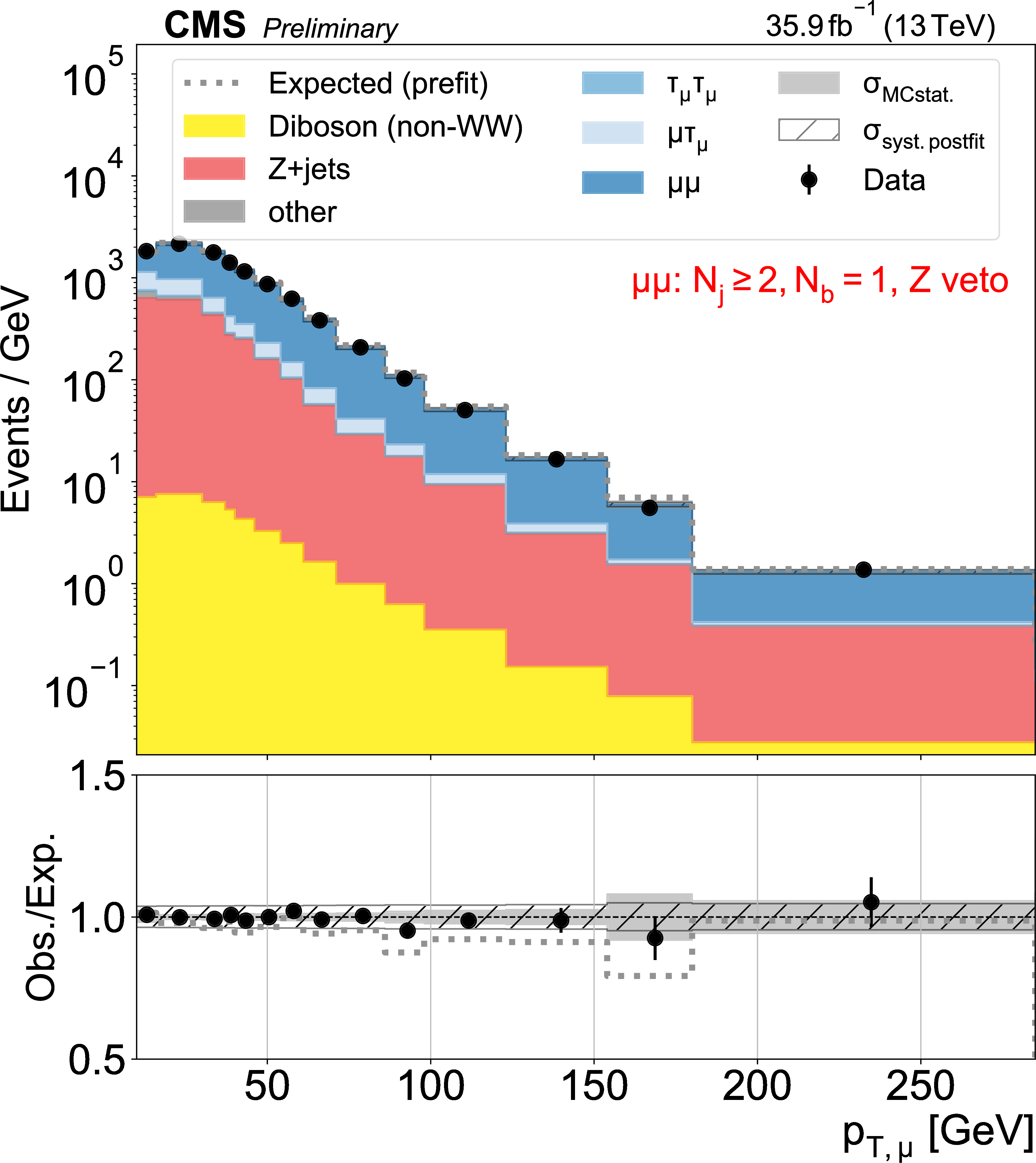
Figure 1-c:
Distributions used as inputs for the binned likelihood fits for the ee (upper) and $\mu \mu $ (lower) categories, with the requirement of one (left) or more than one (right) b-tagged jets. The bottom panels show the ratio of data over prefit (dotted line) and postfit (black circles) expectations, with associated statistical uncertainties (hatched area) and postfit systematic uncertainties (shaded gray). |

png pdf |
Figure 1-d:
Distributions used as inputs for the binned likelihood fits for the ee (upper) and $\mu \mu $ (lower) categories, with the requirement of one (left) or more than one (right) b-tagged jets. The bottom panels show the ratio of data over prefit (dotted line) and postfit (black circles) expectations, with associated statistical uncertainties (hatched area) and postfit systematic uncertainties (shaded gray). |
png pdf |
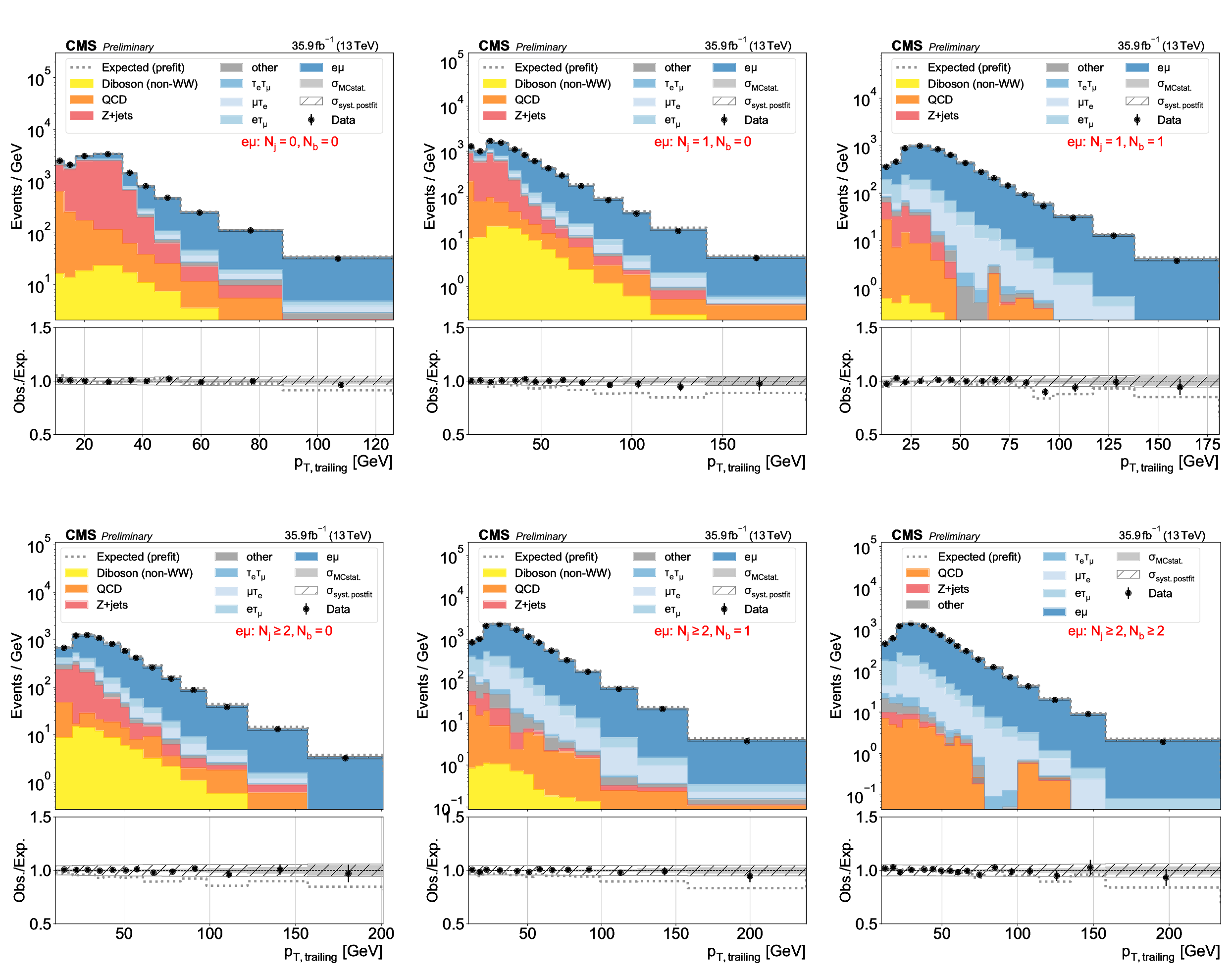
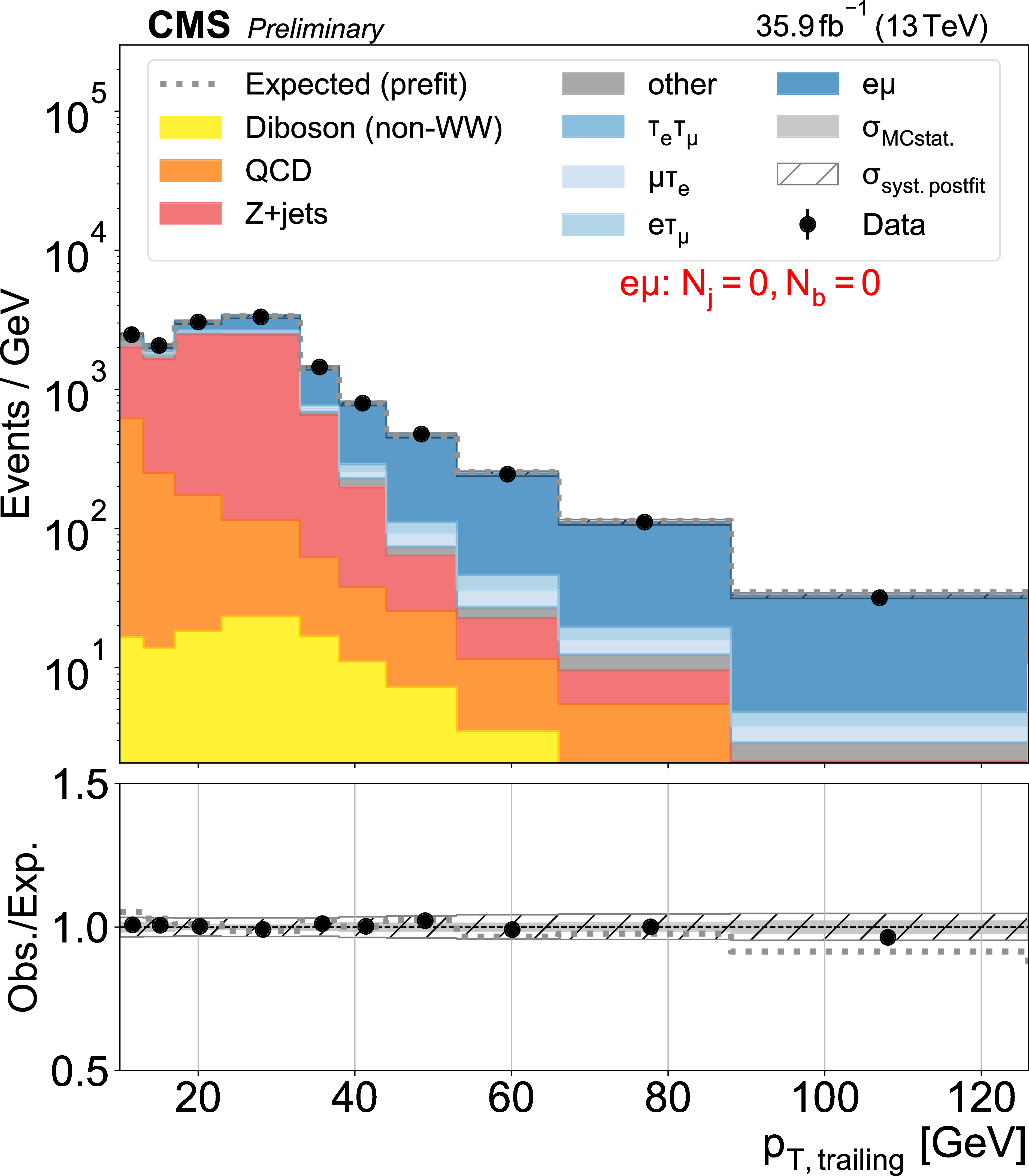
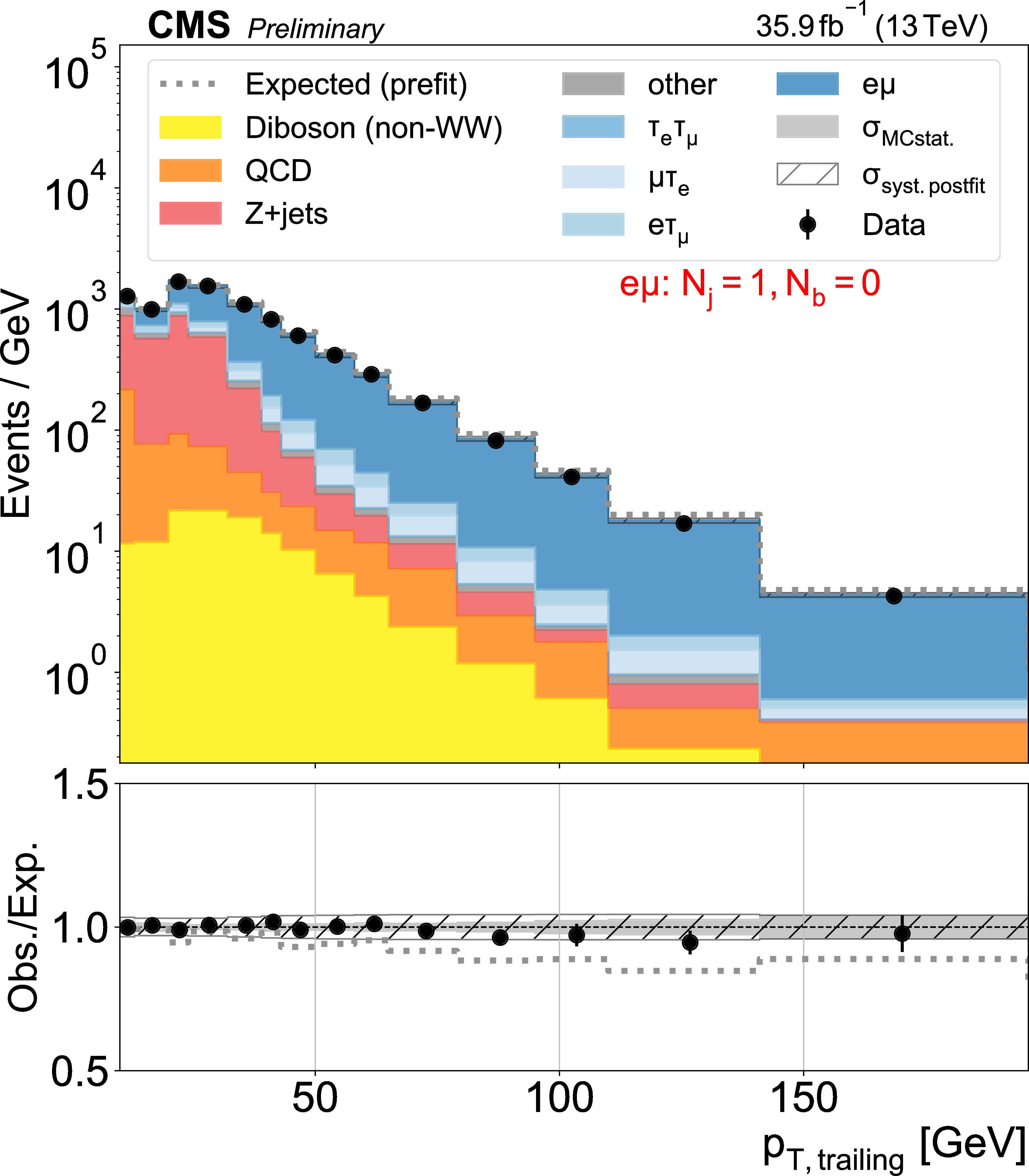
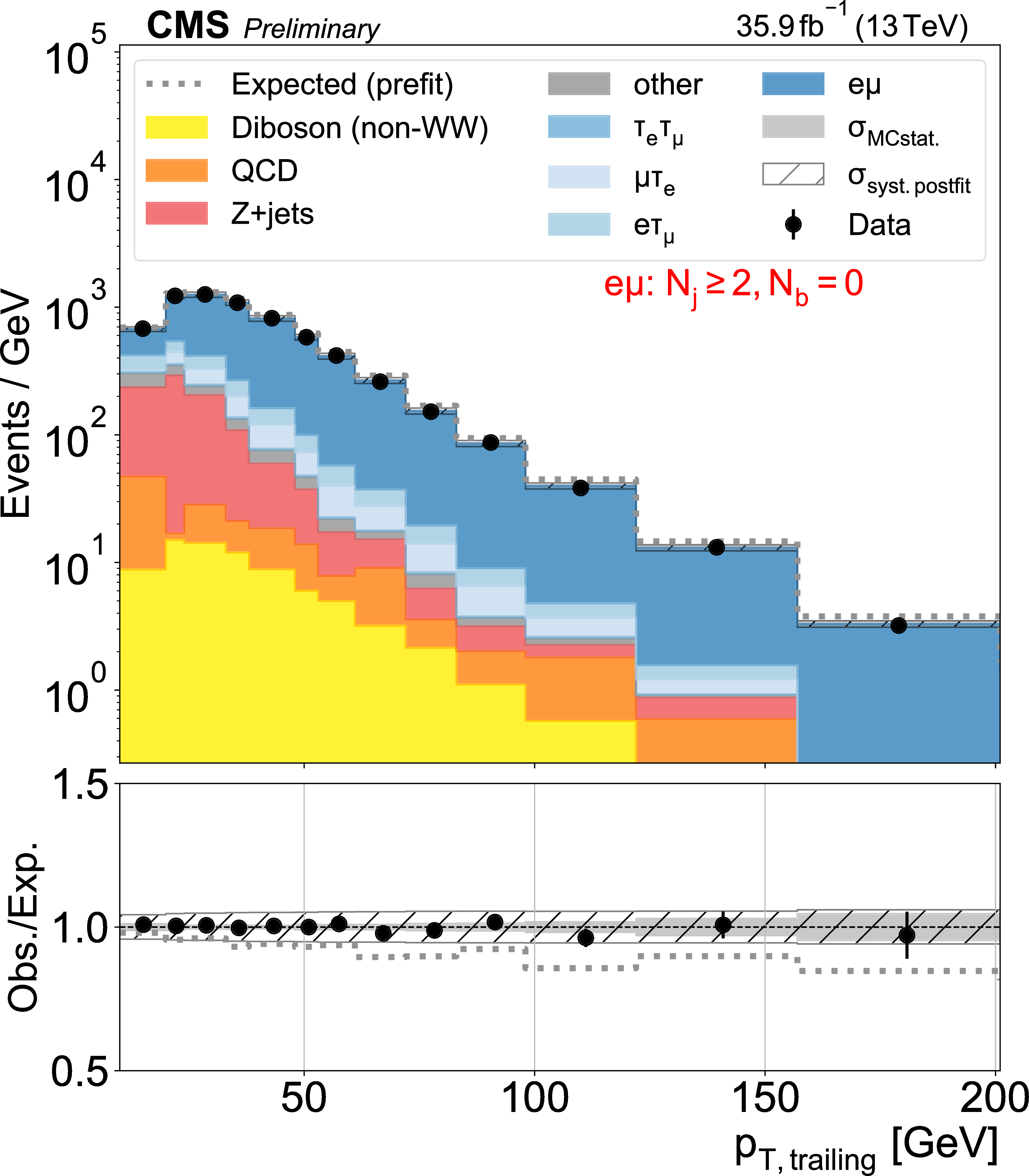
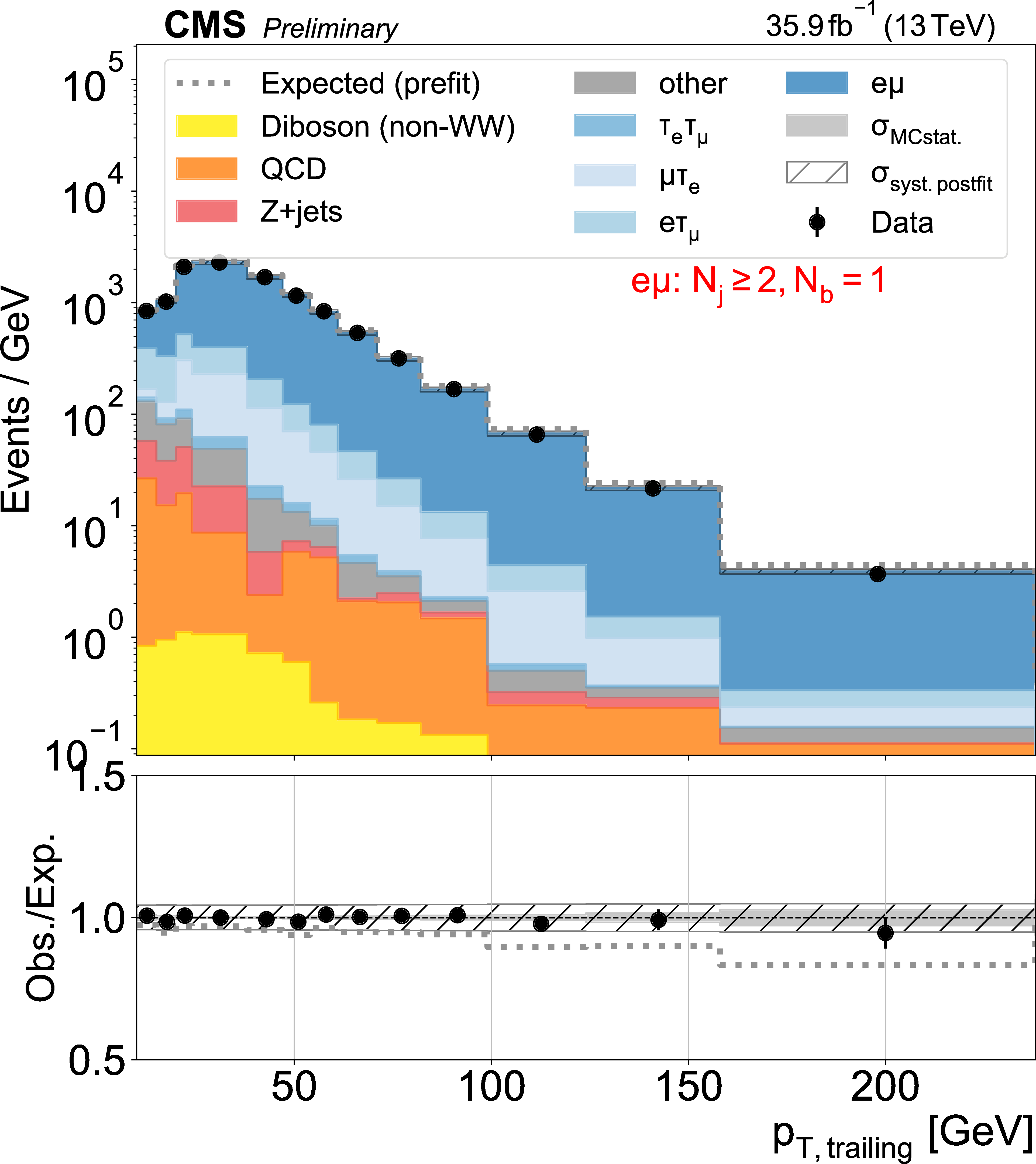
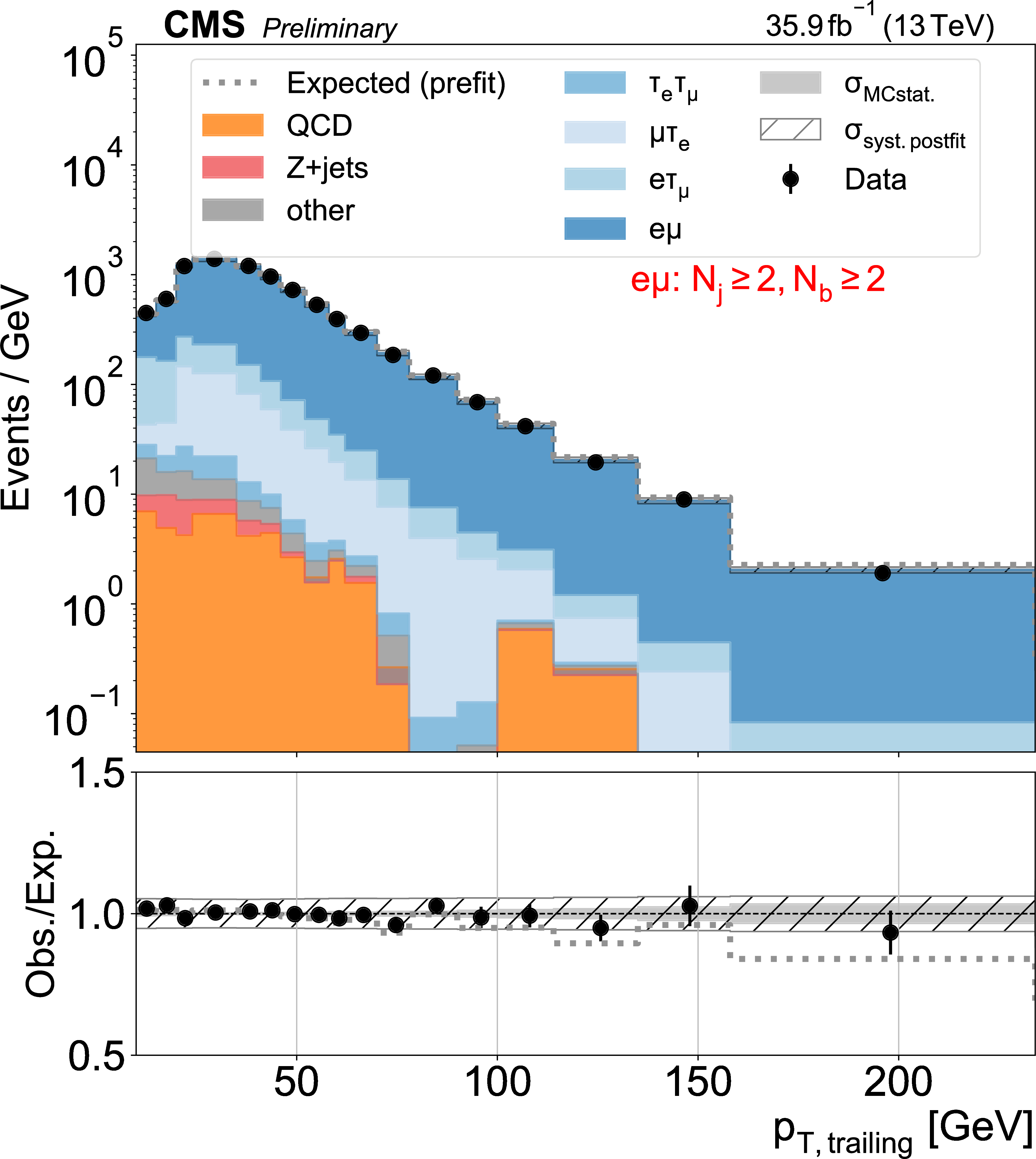
Figure 2:
Distributions used as inputs for the binned likelihood fits for the e$\mu$ categories. The different panels list the varying selections on the number of jets ($N_\mathrm {j}$) and of b-tagged jets ($N_\mathrm{b} $) required in each case. The bottom panels show the ratio of data over prefit expectations, with the gray histograms (slanted bars) indicating MC statistical (postfit systematic) uncertainties. |
png pdf |
Figure 2-a:
Distributions used as inputs for the binned likelihood fits for the e$\mu$ categories. The different panels list the varying selections on the number of jets ($N_\mathrm {j}$) and of b-tagged jets ($N_\mathrm{b} $) required in each case. The bottom panels show the ratio of data over prefit expectations, with the gray histograms (slanted bars) indicating MC statistical (postfit systematic) uncertainties. |
png pdf |
Figure 2-b:
Distributions used as inputs for the binned likelihood fits for the e$\mu$ categories. The different panels list the varying selections on the number of jets ($N_\mathrm {j}$) and of b-tagged jets ($N_\mathrm{b} $) required in each case. The bottom panels show the ratio of data over prefit expectations, with the gray histograms (slanted bars) indicating MC statistical (postfit systematic) uncertainties. |

png pdf |
Figure 2-c:
Distributions used as inputs for the binned likelihood fits for the e$\mu$ categories. The different panels list the varying selections on the number of jets ($N_\mathrm {j}$) and of b-tagged jets ($N_\mathrm{b} $) required in each case. The bottom panels show the ratio of data over prefit expectations, with the gray histograms (slanted bars) indicating MC statistical (postfit systematic) uncertainties. |
png pdf |
Figure 2-d:
Distributions used as inputs for the binned likelihood fits for the e$\mu$ categories. The different panels list the varying selections on the number of jets ($N_\mathrm {j}$) and of b-tagged jets ($N_\mathrm{b} $) required in each case. The bottom panels show the ratio of data over prefit expectations, with the gray histograms (slanted bars) indicating MC statistical (postfit systematic) uncertainties. |
png pdf |
Figure 2-e:
Distributions used as inputs for the binned likelihood fits for the e$\mu$ categories. The different panels list the varying selections on the number of jets ($N_\mathrm {j}$) and of b-tagged jets ($N_\mathrm{b} $) required in each case. The bottom panels show the ratio of data over prefit expectations, with the gray histograms (slanted bars) indicating MC statistical (postfit systematic) uncertainties. |
png pdf |
Figure 2-f:
Distributions used as inputs for the binned likelihood fits for the e$\mu$ categories. The different panels list the varying selections on the number of jets ($N_\mathrm {j}$) and of b-tagged jets ($N_\mathrm{b} $) required in each case. The bottom panels show the ratio of data over prefit expectations, with the gray histograms (slanted bars) indicating MC statistical (postfit systematic) uncertainties. |

png pdf |
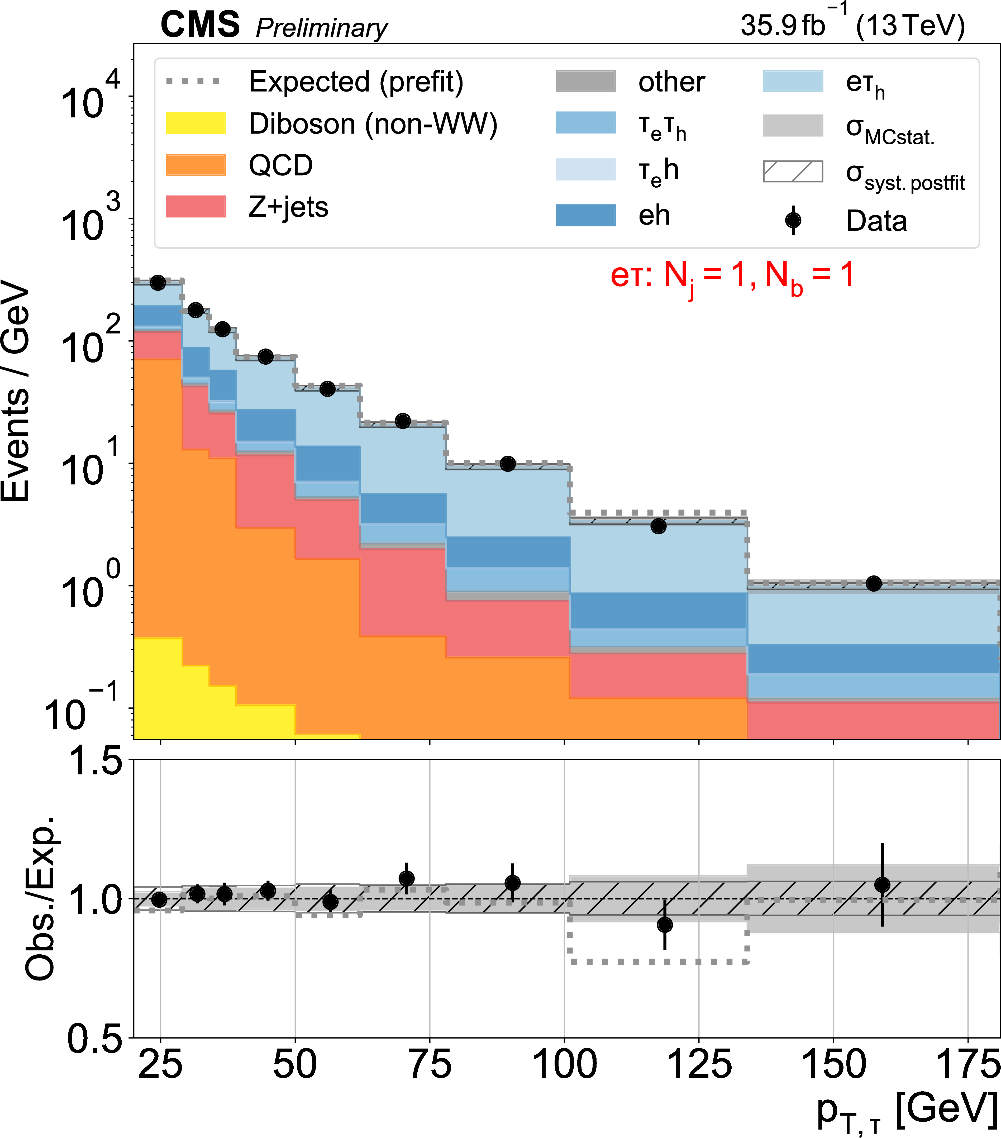
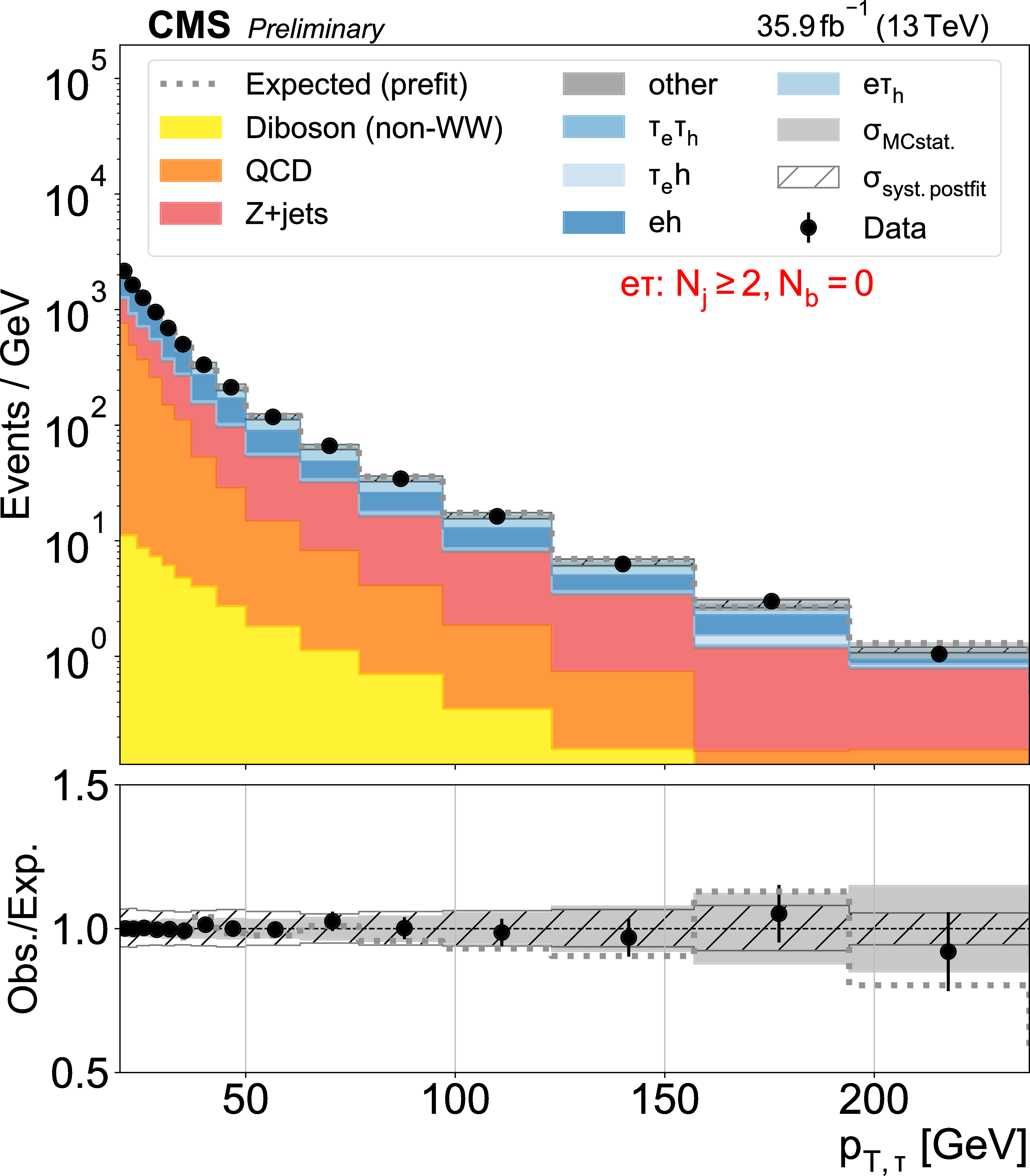
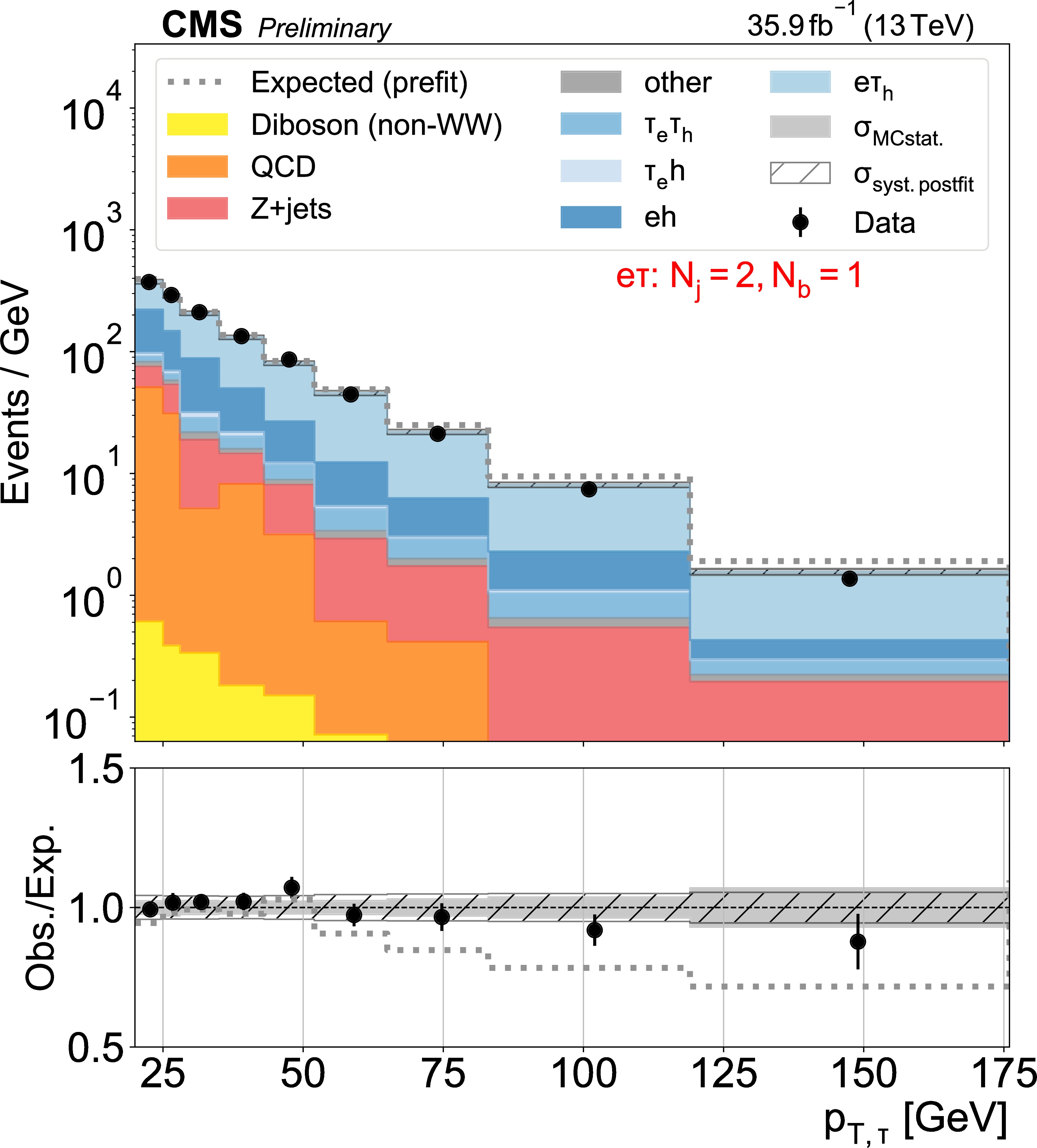
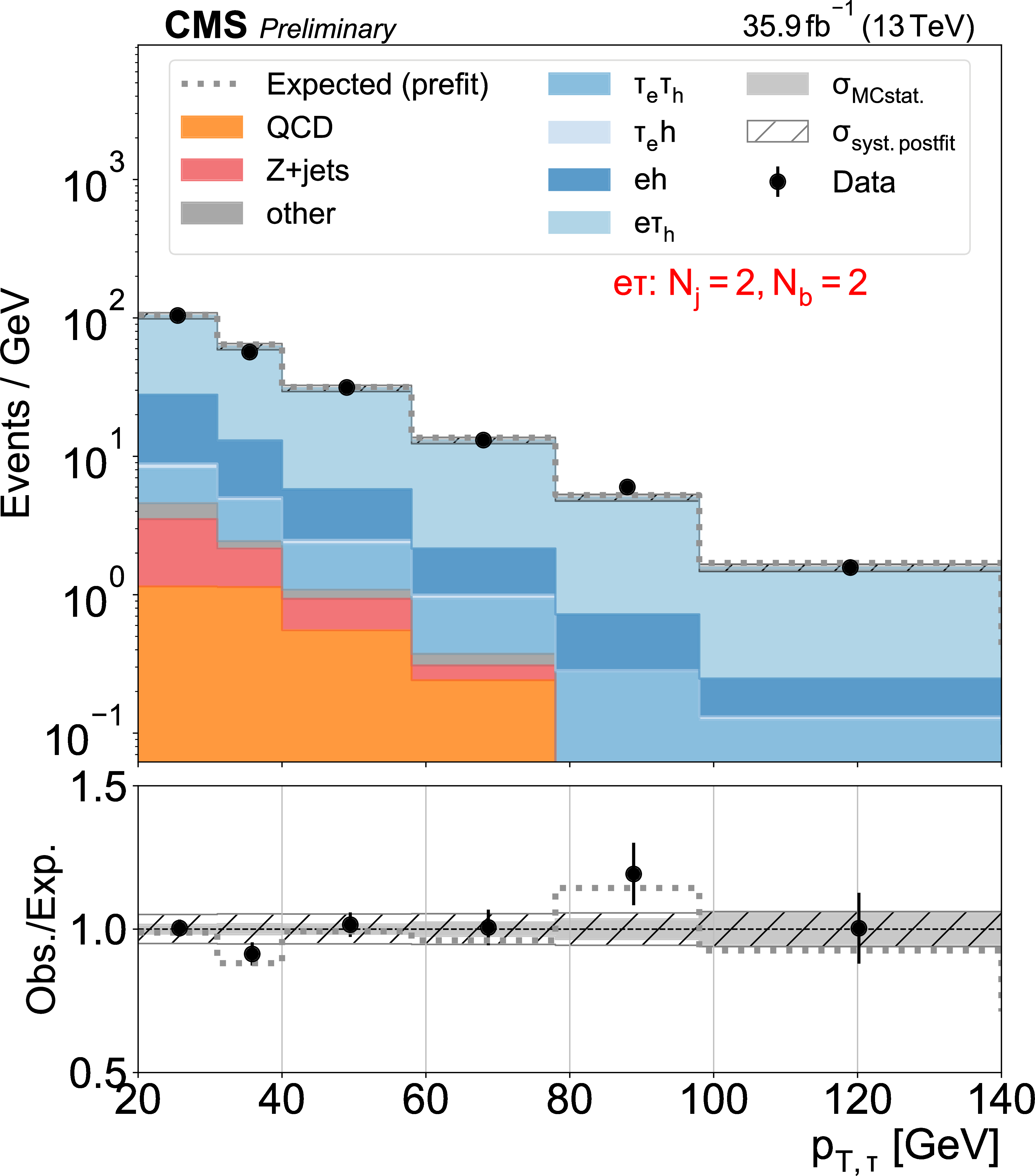
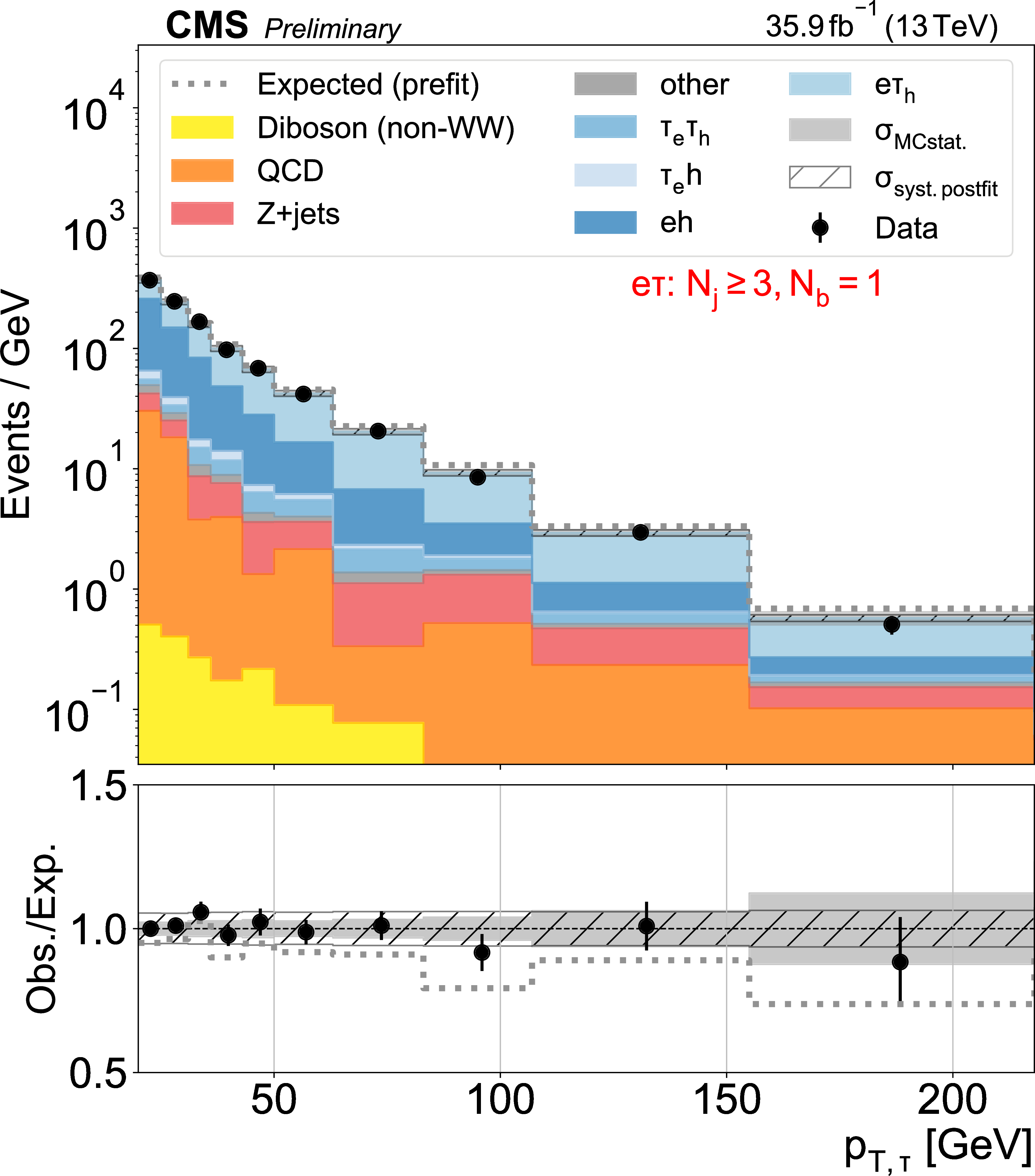
Figure 3:
Distributions used as inputs for the binned likelihood fits for the e$\tau$ categories. The different panels list the varying selections on the number of jets ($N_\mathrm {j}$) and of b-tagged jets ($N_\mathrm{b} $) required in each case. The bottom panels show the ratio of data over prefit expectations, with the gray band (slanted bars) indicating MC statistical (postfit systematic) uncertainties. |

png pdf |
Figure 3-a:
Distributions used as inputs for the binned likelihood fits for the e$\tau$ categories. The different panels list the varying selections on the number of jets ($N_\mathrm {j}$) and of b-tagged jets ($N_\mathrm{b} $) required in each case. The bottom panels show the ratio of data over prefit expectations, with the gray band (slanted bars) indicating MC statistical (postfit systematic) uncertainties. |

png pdf |
Figure 3-b:
Distributions used as inputs for the binned likelihood fits for the e$\tau$ categories. The different panels list the varying selections on the number of jets ($N_\mathrm {j}$) and of b-tagged jets ($N_\mathrm{b} $) required in each case. The bottom panels show the ratio of data over prefit expectations, with the gray band (slanted bars) indicating MC statistical (postfit systematic) uncertainties. |
png pdf |
Figure 3-c:
Distributions used as inputs for the binned likelihood fits for the e$\tau$ categories. The different panels list the varying selections on the number of jets ($N_\mathrm {j}$) and of b-tagged jets ($N_\mathrm{b} $) required in each case. The bottom panels show the ratio of data over prefit expectations, with the gray band (slanted bars) indicating MC statistical (postfit systematic) uncertainties. |
png pdf |
Figure 3-d:
Distributions used as inputs for the binned likelihood fits for the e$\tau$ categories. The different panels list the varying selections on the number of jets ($N_\mathrm {j}$) and of b-tagged jets ($N_\mathrm{b} $) required in each case. The bottom panels show the ratio of data over prefit expectations, with the gray band (slanted bars) indicating MC statistical (postfit systematic) uncertainties. |
png pdf |
Figure 3-e:
Distributions used as inputs for the binned likelihood fits for the e$\tau$ categories. The different panels list the varying selections on the number of jets ($N_\mathrm {j}$) and of b-tagged jets ($N_\mathrm{b} $) required in each case. The bottom panels show the ratio of data over prefit expectations, with the gray band (slanted bars) indicating MC statistical (postfit systematic) uncertainties. |
png pdf |
Figure 3-f:
Distributions used as inputs for the binned likelihood fits for the e$\tau$ categories. The different panels list the varying selections on the number of jets ($N_\mathrm {j}$) and of b-tagged jets ($N_\mathrm{b} $) required in each case. The bottom panels show the ratio of data over prefit expectations, with the gray band (slanted bars) indicating MC statistical (postfit systematic) uncertainties. |
png pdf |
Figure 3-g:
Distributions used as inputs for the binned likelihood fits for the e$\tau$ categories. The different panels list the varying selections on the number of jets ($N_\mathrm {j}$) and of b-tagged jets ($N_\mathrm{b} $) required in each case. The bottom panels show the ratio of data over prefit expectations, with the gray band (slanted bars) indicating MC statistical (postfit systematic) uncertainties. |

png pdf |
Figure 3-h:
Distributions used as inputs for the binned likelihood fits for the e$\tau$ categories. The different panels list the varying selections on the number of jets ($N_\mathrm {j}$) and of b-tagged jets ($N_\mathrm{b} $) required in each case. The bottom panels show the ratio of data over prefit expectations, with the gray band (slanted bars) indicating MC statistical (postfit systematic) uncertainties. |

png pdf |
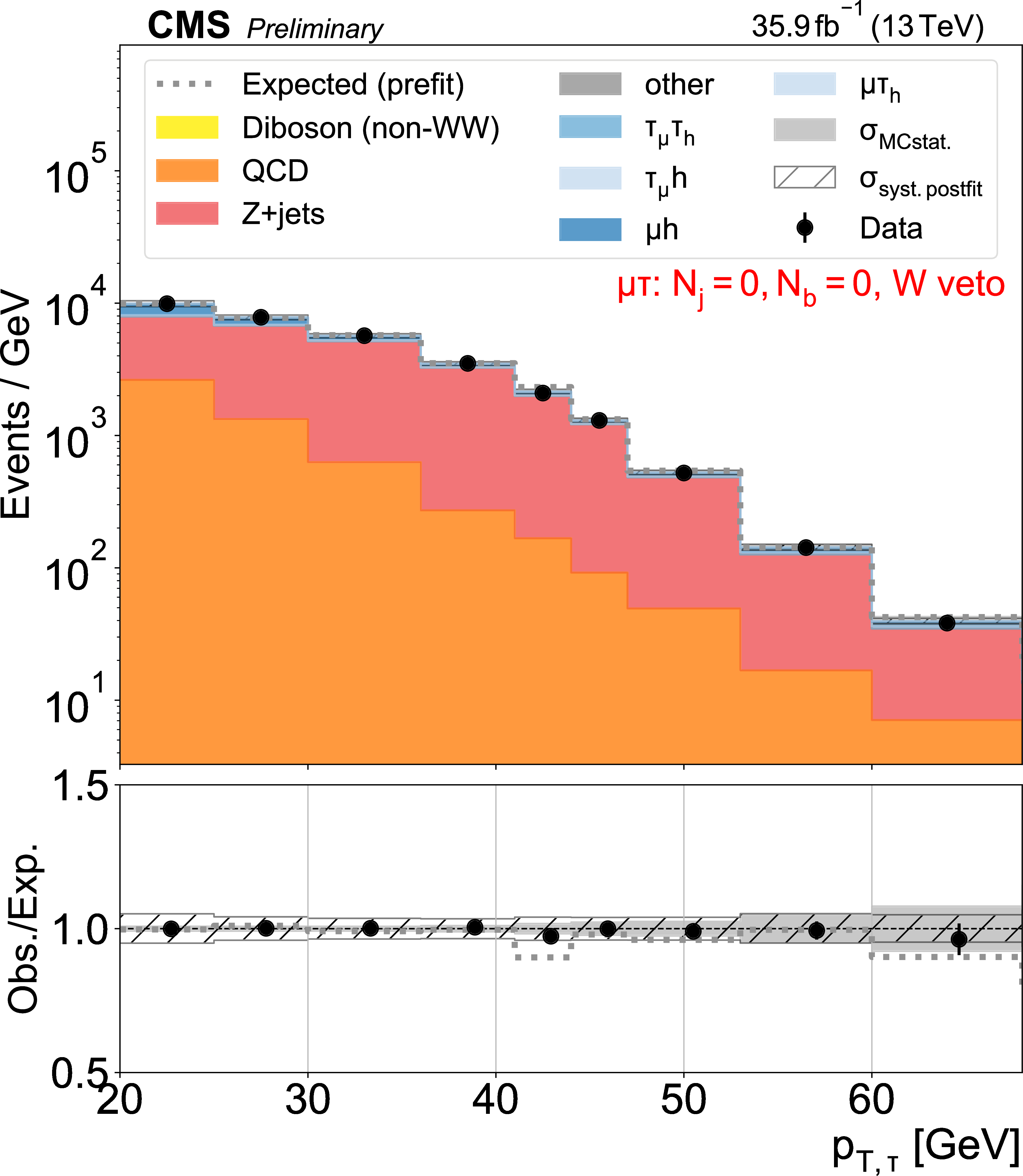
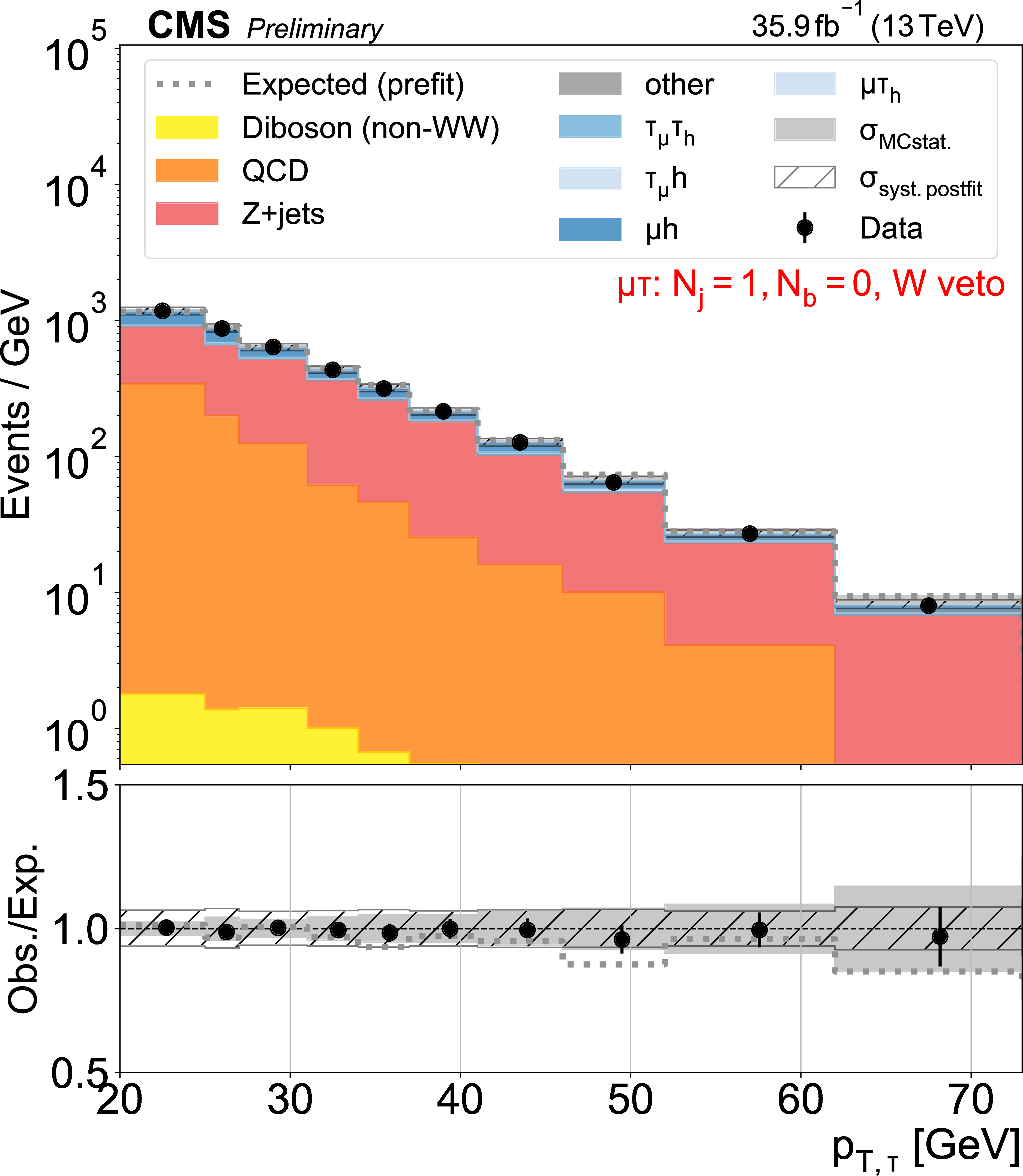
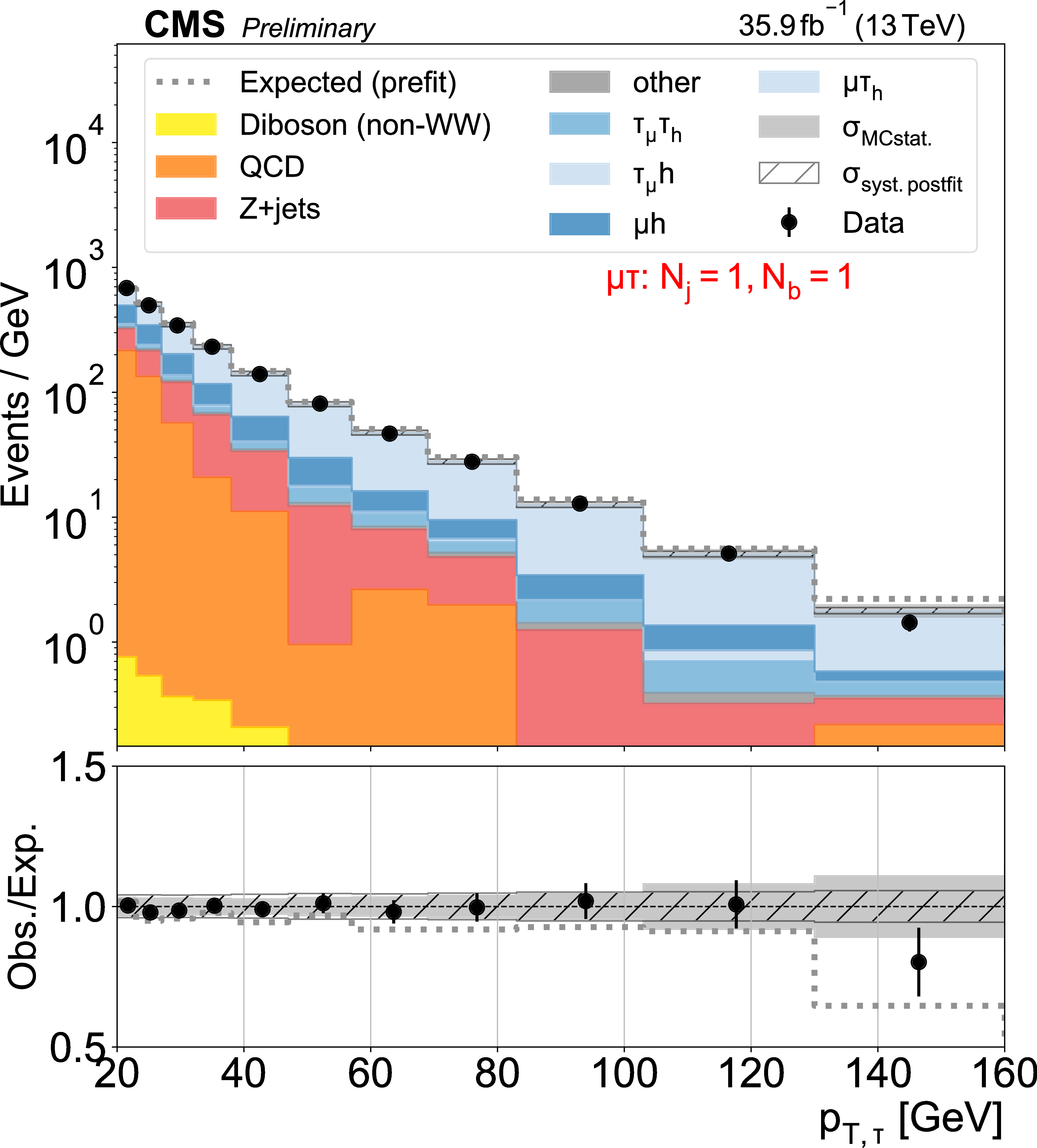
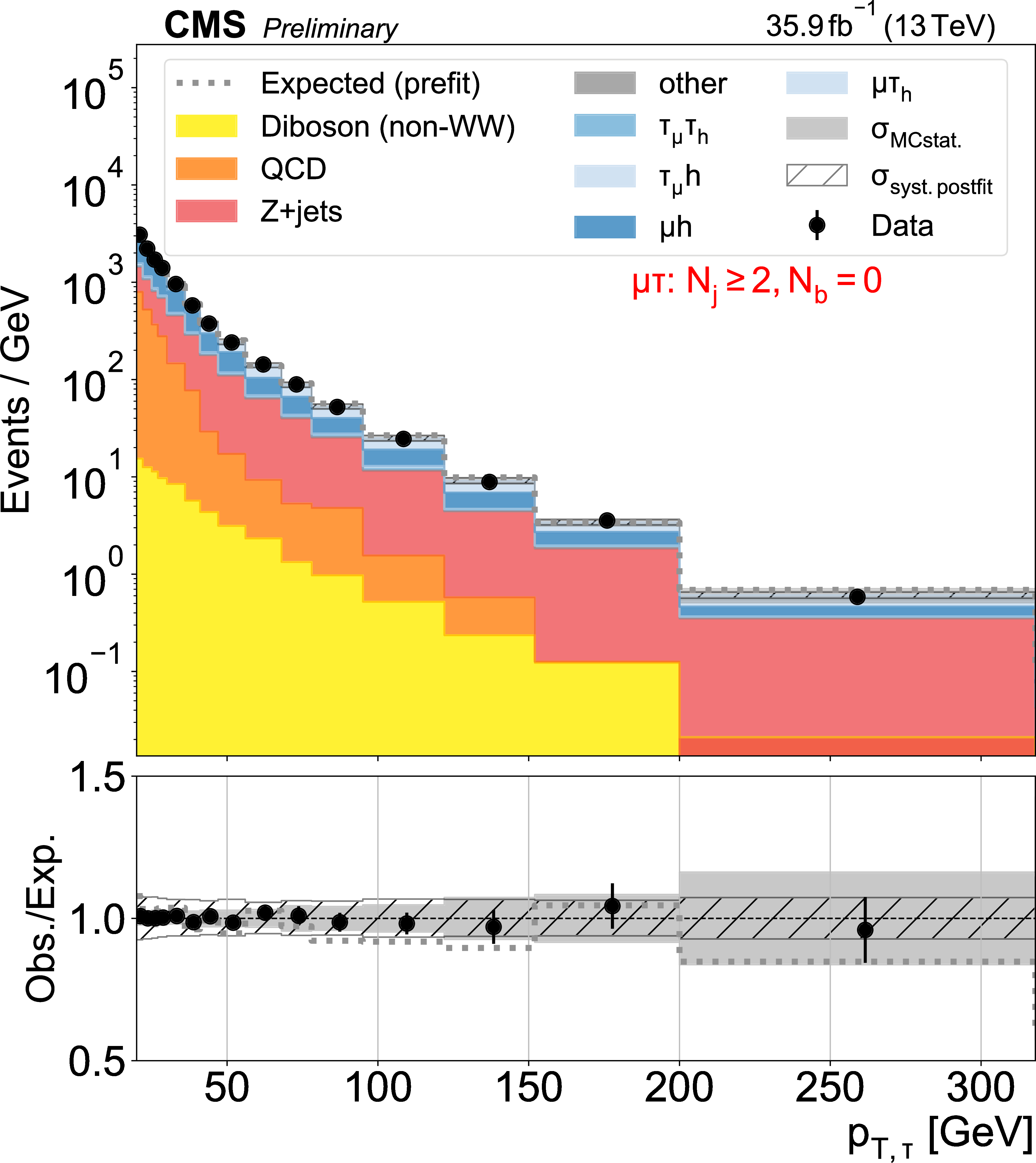
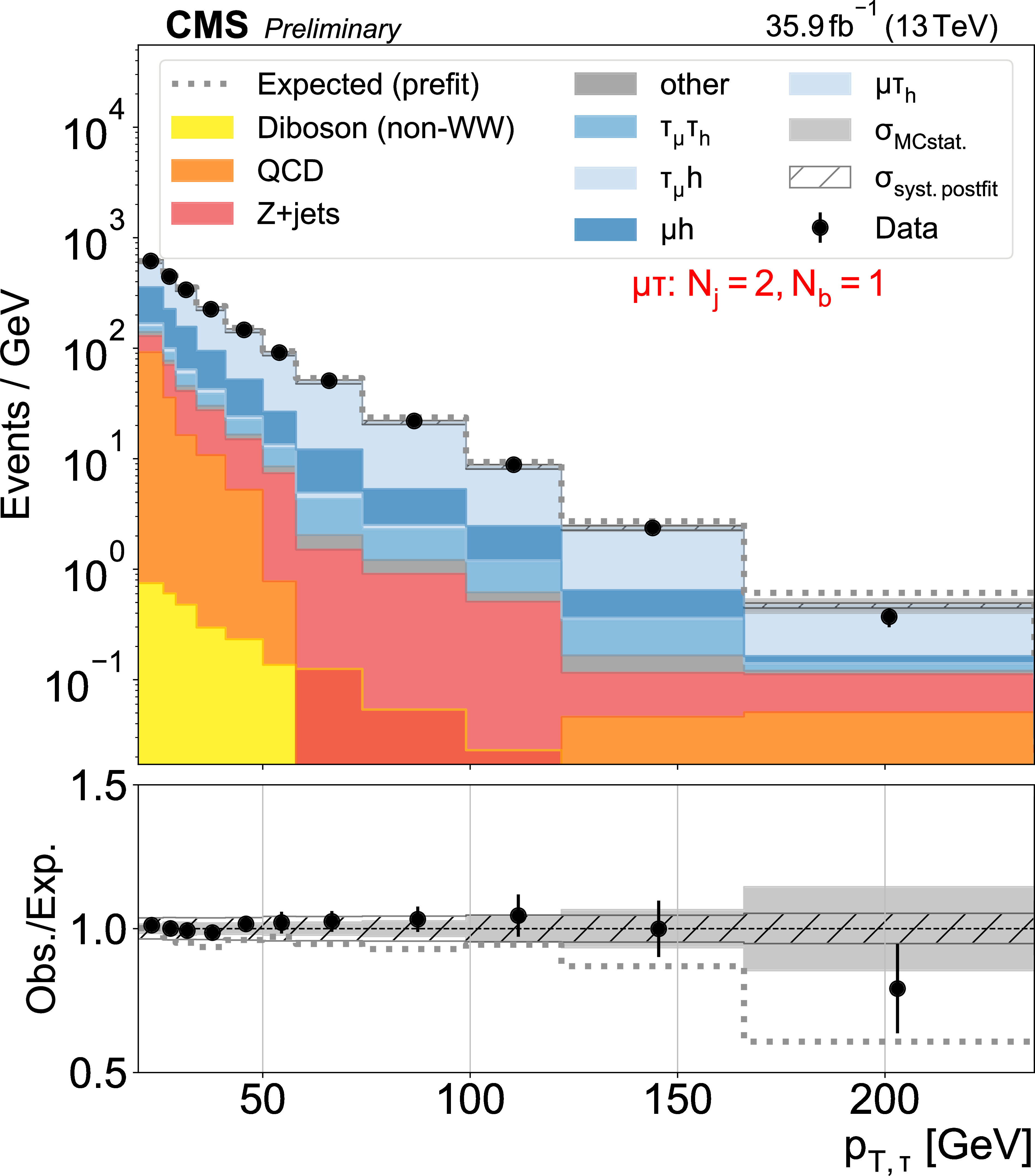
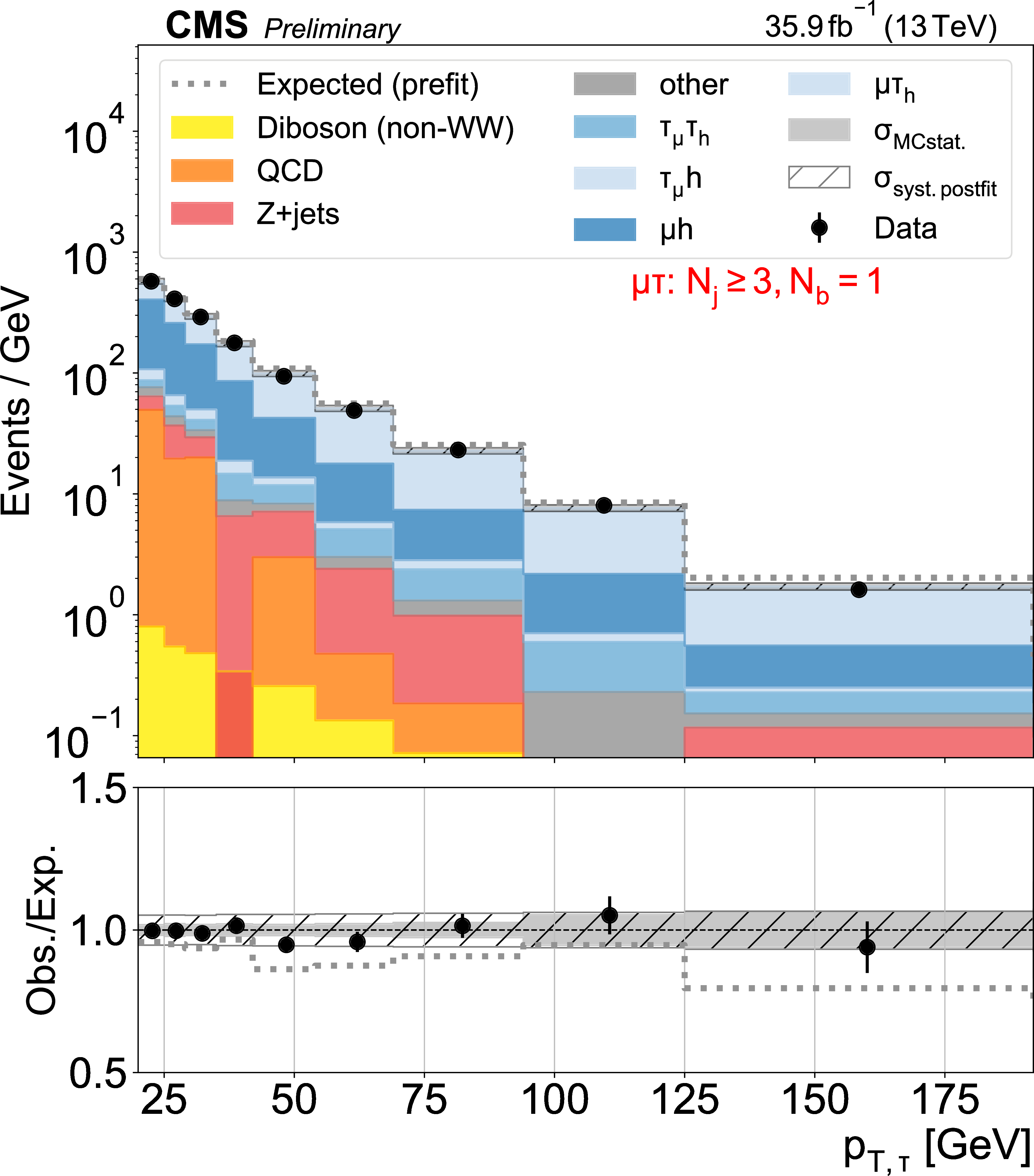
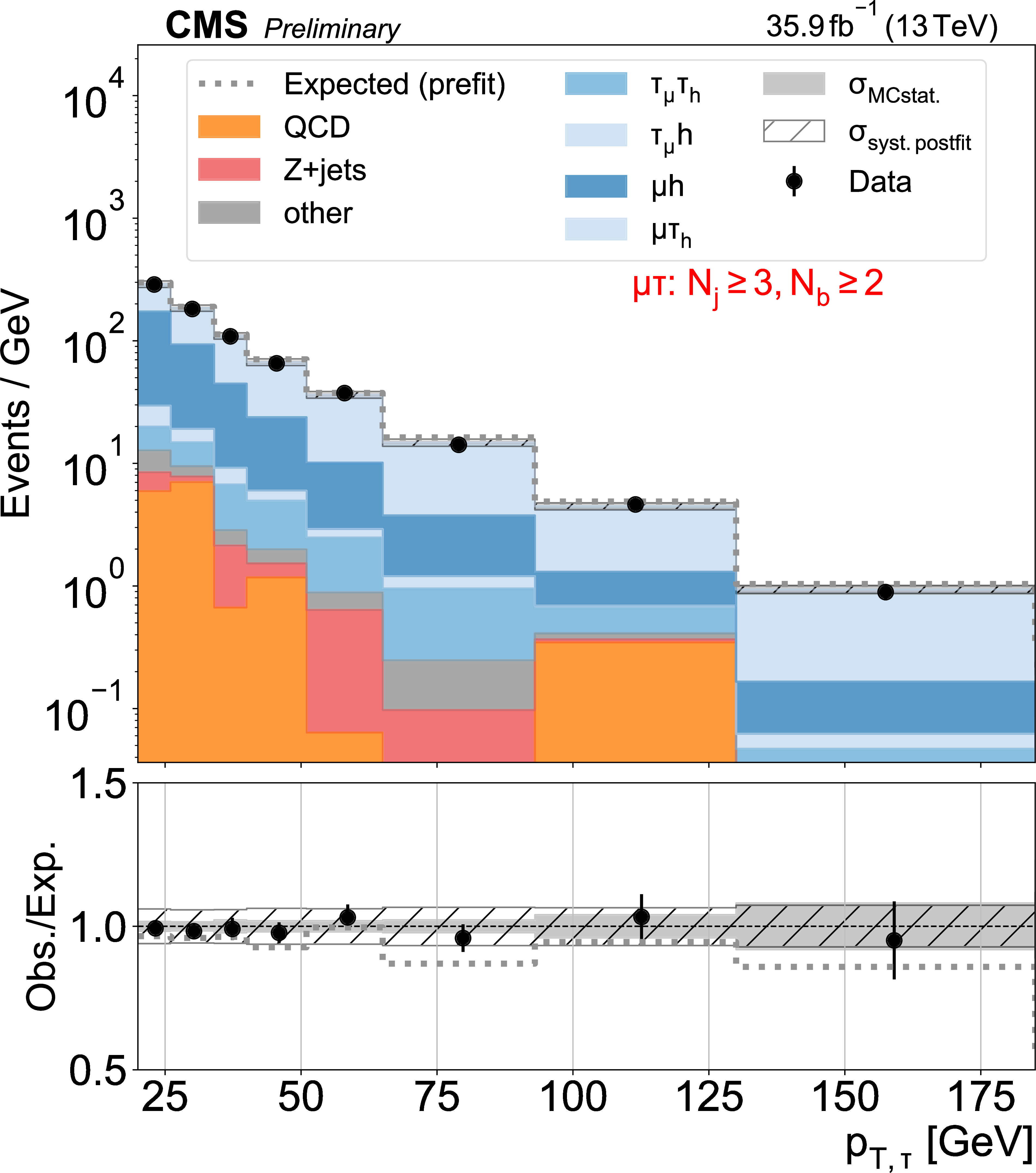
Figure 4:
Distributions used as inputs for the binned likelihood fits for the $\mu \tau $ categories. The different panels list the varying selections on the number of jets ($N_\mathrm {j}$) and of b-tagged jets ($N_\mathrm{b} $) required in each case. The bottom panels show the ratio of data over prefit expectations, with the gray histograms (slanted bars) indicating MC statistical (postfit systematic) uncertainties. |
png pdf |
Figure 4-a:
Distributions used as inputs for the binned likelihood fits for the $\mu \tau $ categories. The different panels list the varying selections on the number of jets ($N_\mathrm {j}$) and of b-tagged jets ($N_\mathrm{b} $) required in each case. The bottom panels show the ratio of data over prefit expectations, with the gray histograms (slanted bars) indicating MC statistical (postfit systematic) uncertainties. |
png pdf |
Figure 4-b:
Distributions used as inputs for the binned likelihood fits for the $\mu \tau $ categories. The different panels list the varying selections on the number of jets ($N_\mathrm {j}$) and of b-tagged jets ($N_\mathrm{b} $) required in each case. The bottom panels show the ratio of data over prefit expectations, with the gray histograms (slanted bars) indicating MC statistical (postfit systematic) uncertainties. |
png pdf |
Figure 4-c:
Distributions used as inputs for the binned likelihood fits for the $\mu \tau $ categories. The different panels list the varying selections on the number of jets ($N_\mathrm {j}$) and of b-tagged jets ($N_\mathrm{b} $) required in each case. The bottom panels show the ratio of data over prefit expectations, with the gray histograms (slanted bars) indicating MC statistical (postfit systematic) uncertainties. |
png pdf |
Figure 4-d:
Distributions used as inputs for the binned likelihood fits for the $\mu \tau $ categories. The different panels list the varying selections on the number of jets ($N_\mathrm {j}$) and of b-tagged jets ($N_\mathrm{b} $) required in each case. The bottom panels show the ratio of data over prefit expectations, with the gray histograms (slanted bars) indicating MC statistical (postfit systematic) uncertainties. |
png pdf |
Figure 4-e:
Distributions used as inputs for the binned likelihood fits for the $\mu \tau $ categories. The different panels list the varying selections on the number of jets ($N_\mathrm {j}$) and of b-tagged jets ($N_\mathrm{b} $) required in each case. The bottom panels show the ratio of data over prefit expectations, with the gray histograms (slanted bars) indicating MC statistical (postfit systematic) uncertainties. |

png pdf |
Figure 4-f:
Distributions used as inputs for the binned likelihood fits for the $\mu \tau $ categories. The different panels list the varying selections on the number of jets ($N_\mathrm {j}$) and of b-tagged jets ($N_\mathrm{b} $) required in each case. The bottom panels show the ratio of data over prefit expectations, with the gray histograms (slanted bars) indicating MC statistical (postfit systematic) uncertainties. |
png pdf |
Figure 4-g:
Distributions used as inputs for the binned likelihood fits for the $\mu \tau $ categories. The different panels list the varying selections on the number of jets ($N_\mathrm {j}$) and of b-tagged jets ($N_\mathrm{b} $) required in each case. The bottom panels show the ratio of data over prefit expectations, with the gray histograms (slanted bars) indicating MC statistical (postfit systematic) uncertainties. |
png pdf |
Figure 4-h:
Distributions used as inputs for the binned likelihood fits for the $\mu \tau $ categories. The different panels list the varying selections on the number of jets ($N_\mathrm {j}$) and of b-tagged jets ($N_\mathrm{b} $) required in each case. The bottom panels show the ratio of data over prefit expectations, with the gray histograms (slanted bars) indicating MC statistical (postfit systematic) uncertainties. |
png pdf |
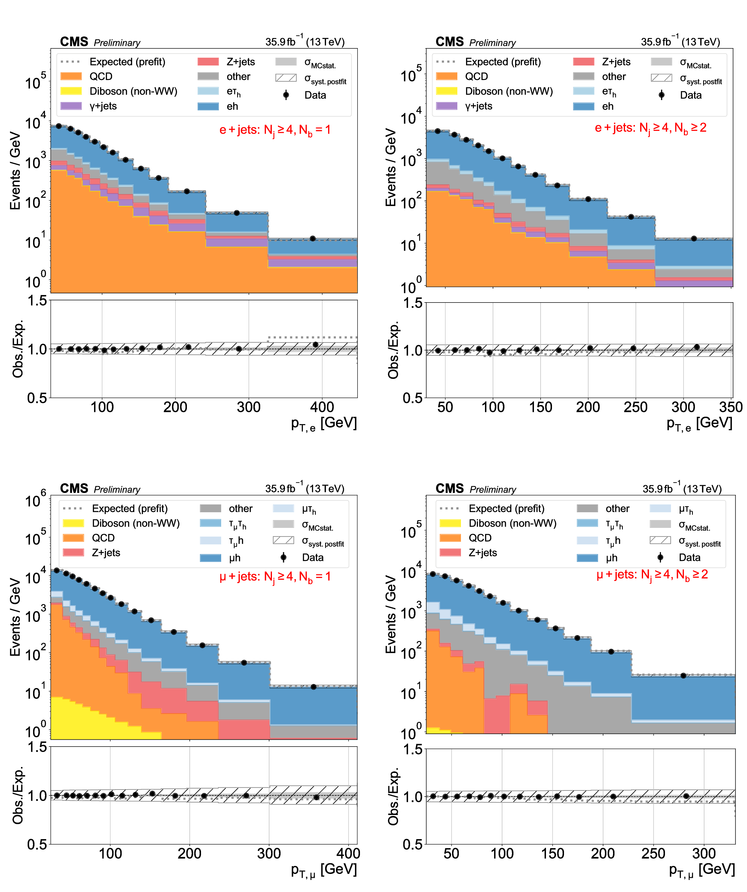
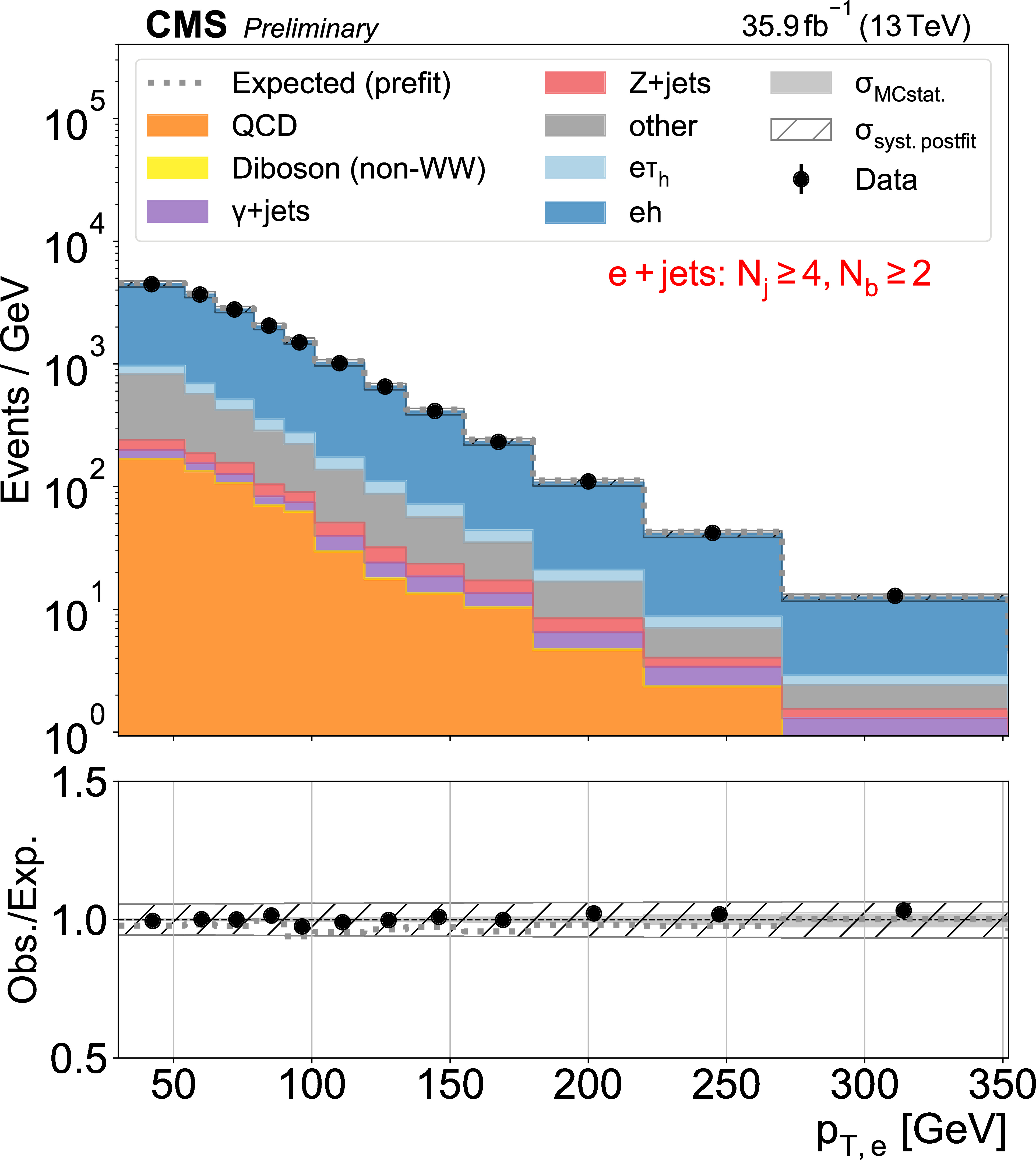
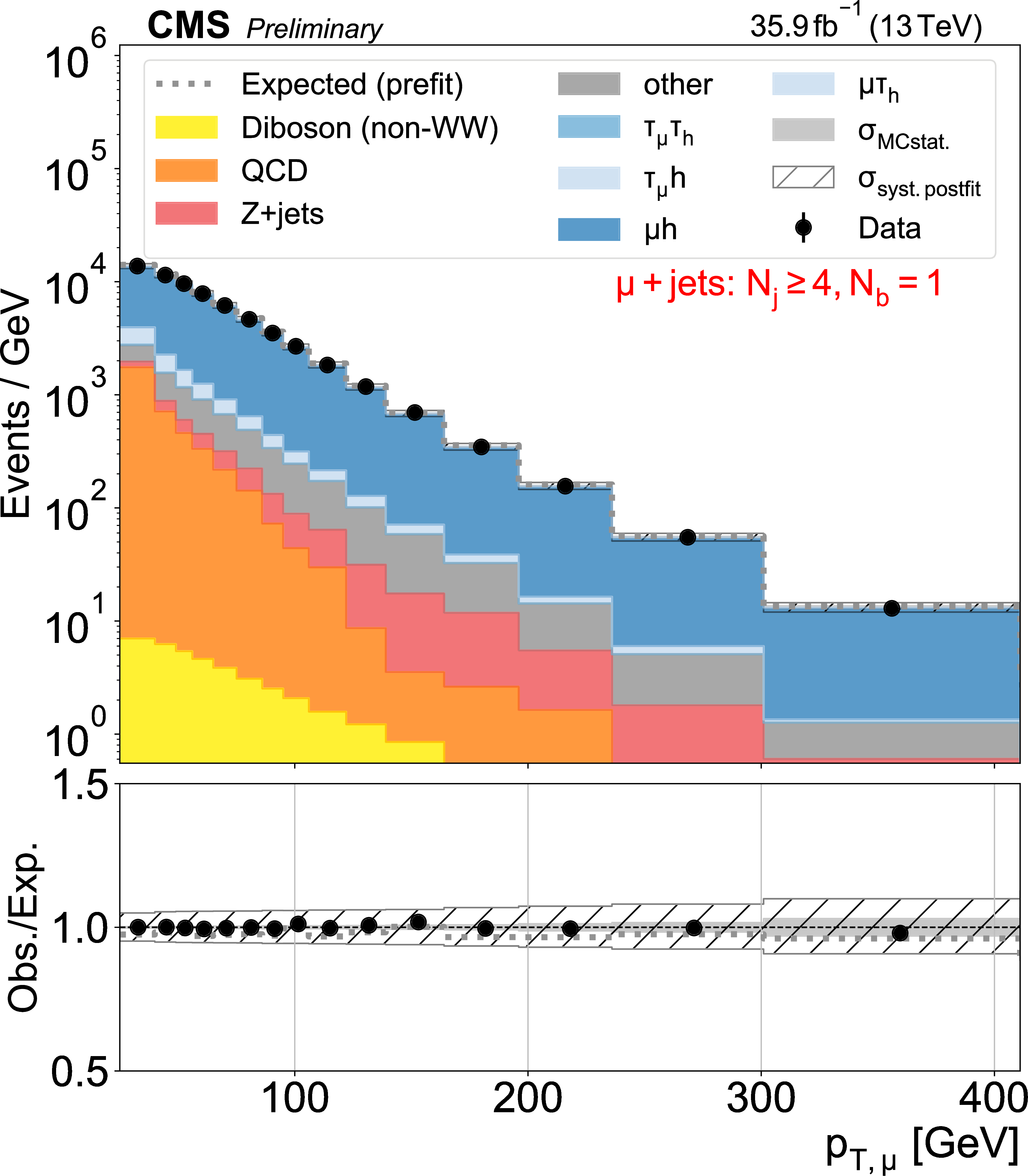
Figure 5:
Distributions used as inputs for the binned likelihood fits for the eh (upper) and $\mu$h (lower) categories, with the requirement of one (left) or more than one (right) b-tagged jets. The bottom panels show the ratio of data over prefit expectations, with the gray histograms (slanted bars) indicating MC statistical (postfit systematic) uncertainties. |

png pdf |
Figure 5-a:
Distributions used as inputs for the binned likelihood fits for the eh (upper) and $\mu$h (lower) categories, with the requirement of one (left) or more than one (right) b-tagged jets. The bottom panels show the ratio of data over prefit expectations, with the gray histograms (slanted bars) indicating MC statistical (postfit systematic) uncertainties. |
png pdf |
Figure 5-b:
Distributions used as inputs for the binned likelihood fits for the eh (upper) and $\mu$h (lower) categories, with the requirement of one (left) or more than one (right) b-tagged jets. The bottom panels show the ratio of data over prefit expectations, with the gray histograms (slanted bars) indicating MC statistical (postfit systematic) uncertainties. |
png pdf |
Figure 5-c:
Distributions used as inputs for the binned likelihood fits for the eh (upper) and $\mu$h (lower) categories, with the requirement of one (left) or more than one (right) b-tagged jets. The bottom panels show the ratio of data over prefit expectations, with the gray histograms (slanted bars) indicating MC statistical (postfit systematic) uncertainties. |
png pdf |
Figure 5-d:
Distributions used as inputs for the binned likelihood fits for the eh (upper) and $\mu$h (lower) categories, with the requirement of one (left) or more than one (right) b-tagged jets. The bottom panels show the ratio of data over prefit expectations, with the gray histograms (slanted bars) indicating MC statistical (postfit systematic) uncertainties. |
png pdf |
Figure 6:
Pulls and impacts of the nuisance parameters on each W leptonic branching fraction. The impacts are calculated with respect to the uncertainty of the corresponding branching fraction component. Error bars on the pull distribution correspond to the postfit uncertainty of the corresponding nuisance parameter. |
png pdf |
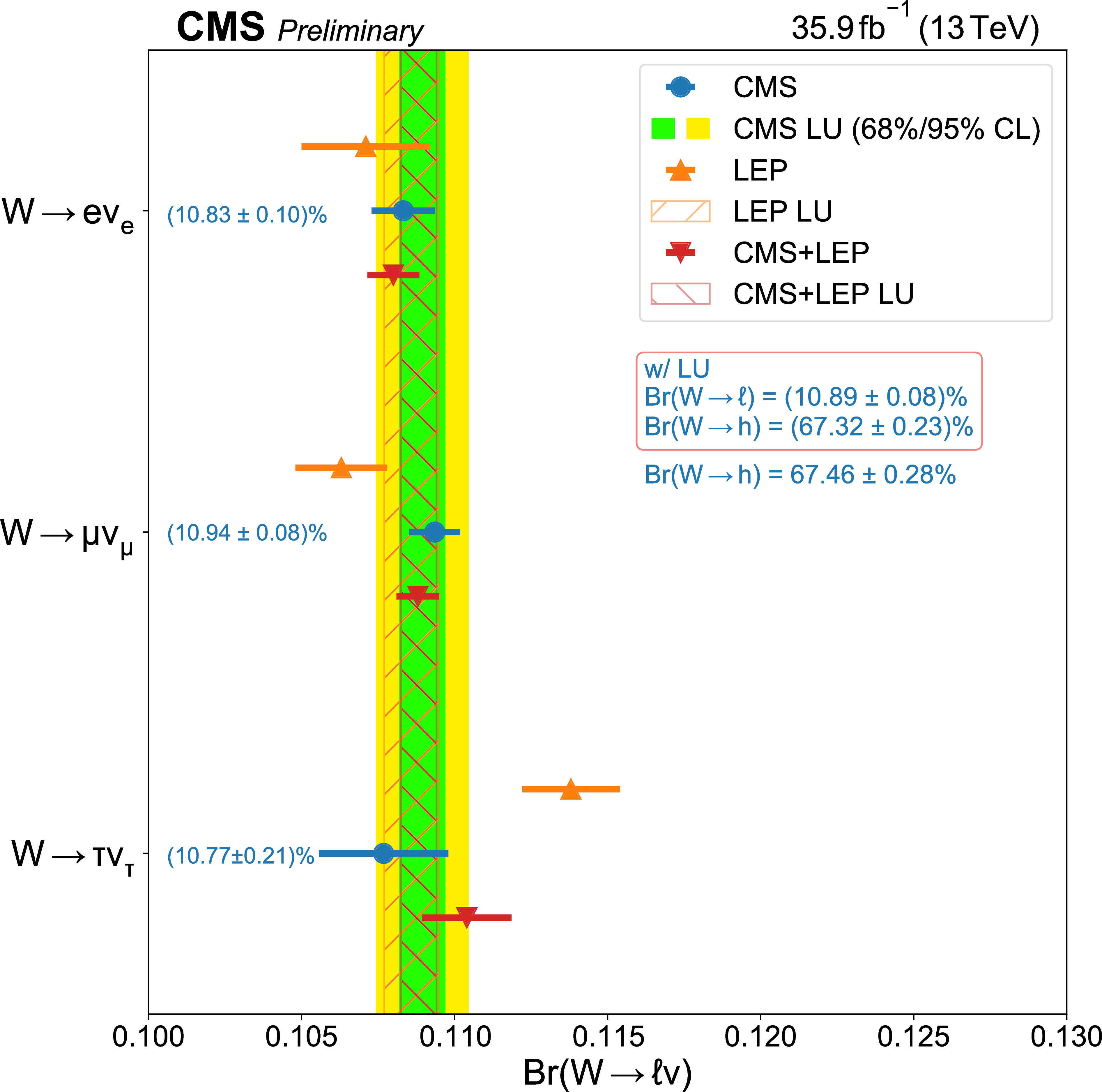
Figure 7:
Summary of the measured values of the W leptonic branching fractions compared to the corresponding LEP results [3]. The vertical green-yellow band shows the extracted W leptonic branching fraction assuming lepton universality (the hatched band shows the corresponding LEP result). |
png pdf |
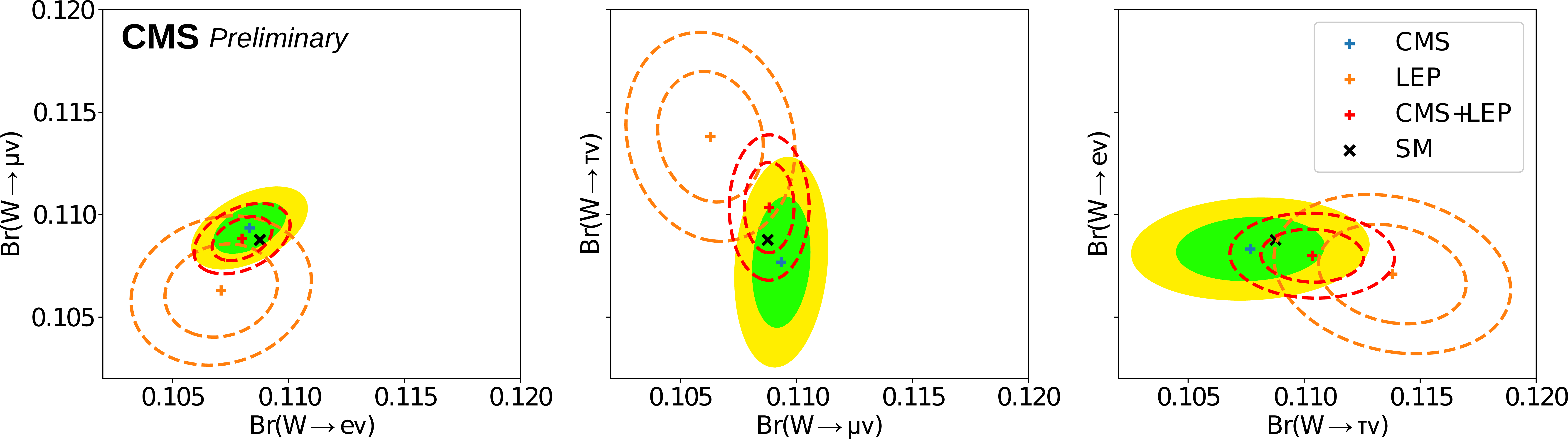
Figure 8:
Two-dimensional comparisons of pairs of W leptonic branching fractions derived here, compared to LEP results and to the SM expectation. The green and yellow bands (dashed lines for the LEP results) correspond to the 68% and 95% CL for the resulting two-dimensional Gaussian distribution. |
png pdf |
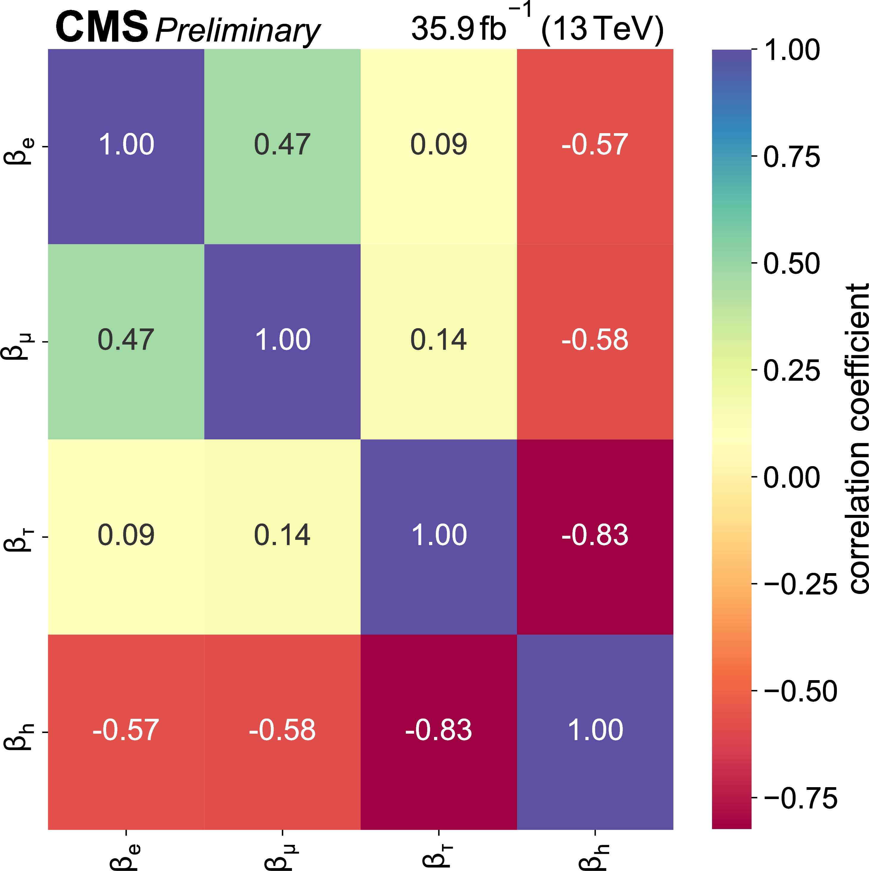
Figure 9:
Correlation matrix between the four W boson decay branching fraction components extracted in this work. |
png pdf |
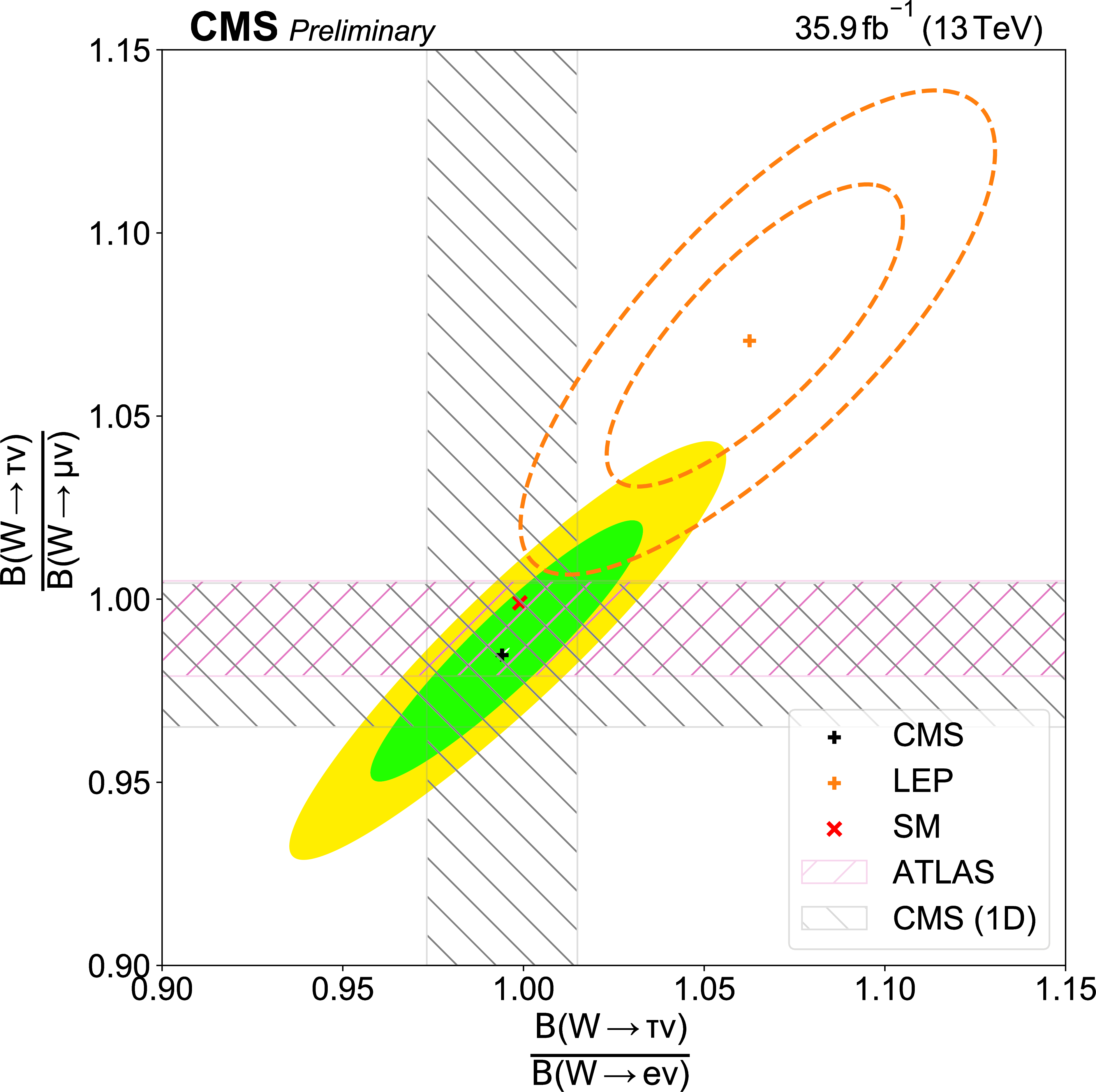
Figure 10:
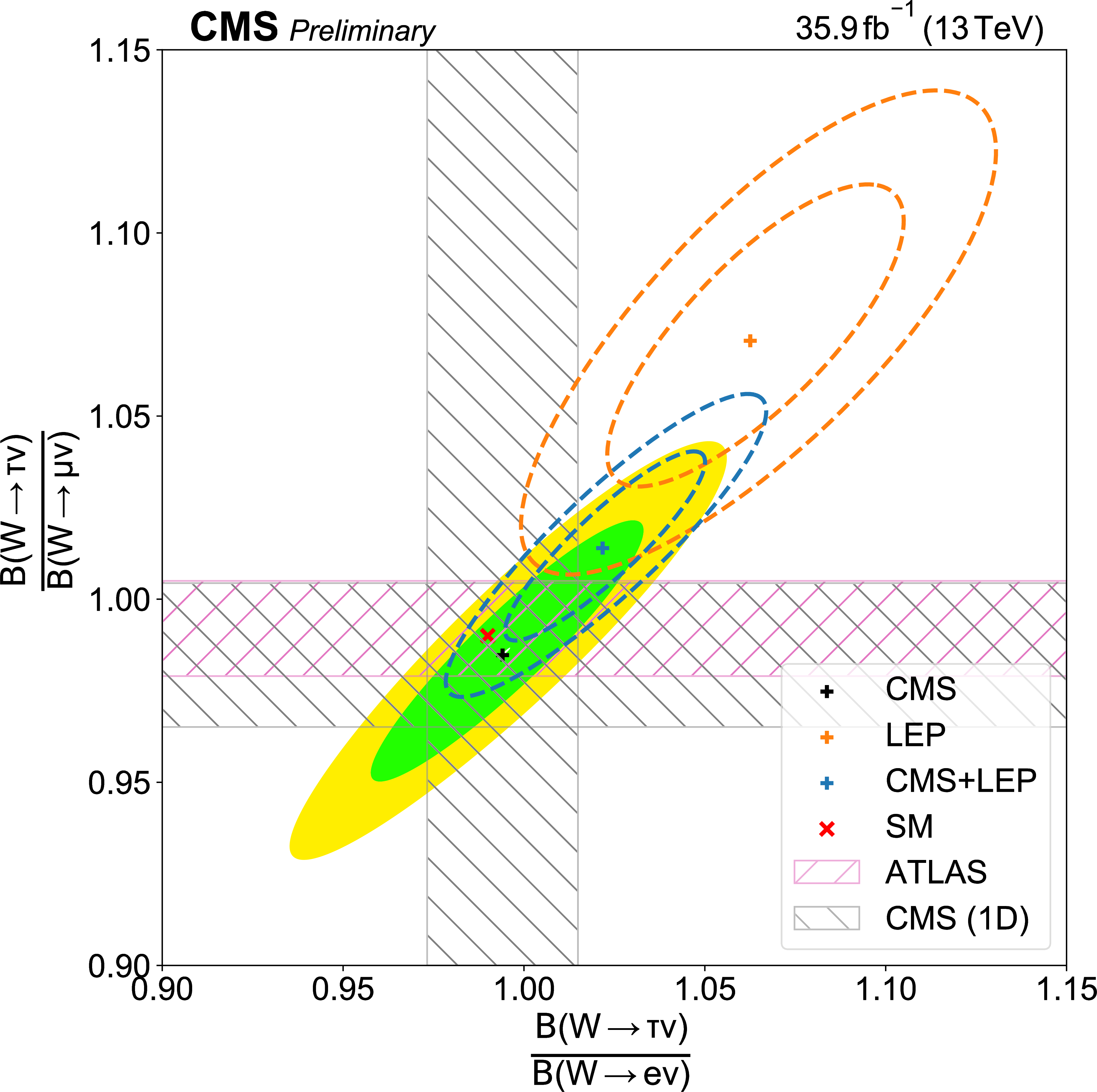
Two-dimensional distributions of the ratios $R_{\tau /\mathrm{e}}$ versus $R_{\tau /\mu}$, compared to similar LEP and ATLAS results and to the SM expectation. The green and yellow bands (dashed lines for the LEP results) correspond to the 68% and 95% CL for the resulting two-dimensional Gaussian distribution. The one-dimensional (1D) 68% CL bands are also overlaid for a better visual comparison with the corresponding ATLAS $R_{\tau /\mu}$ result. |
| Tables | |
png pdf |
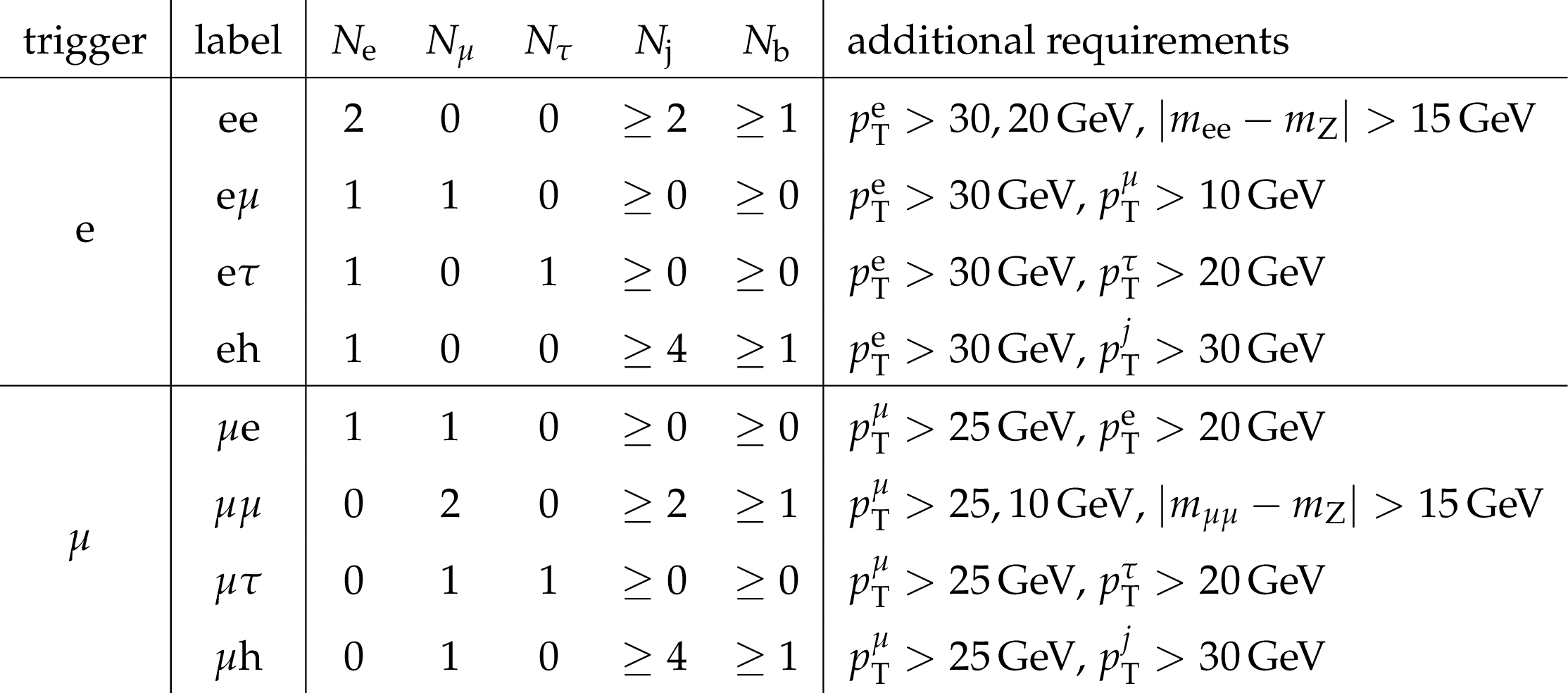
Table 1:
Baseline categorization of events based on the triggering electron or muon, the presence (or vetoing) of isolated reconstructed charged leptons, plus additional jets, identified or not as originating from a b quark. Kinematic criteria required on the charged leptons and jets are listed in the last column. Categories without hadrons in the final state require also the selected leptons to have opposite-sign charge. |
png pdf |
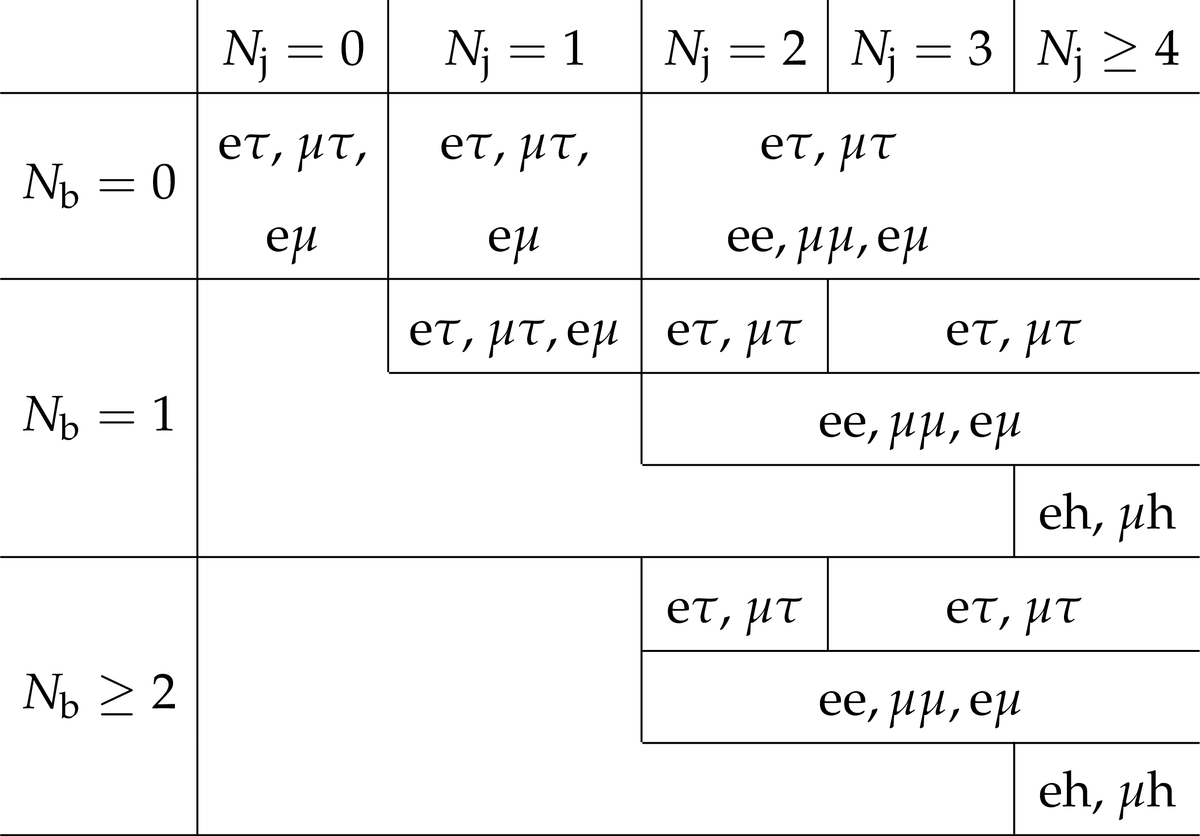
Table 2:
Categorization of events with electron, muon, and/or tau leptons passing the reconstruction criteria, based on their jet and b-tagged jet multiplicities. |
png pdf |
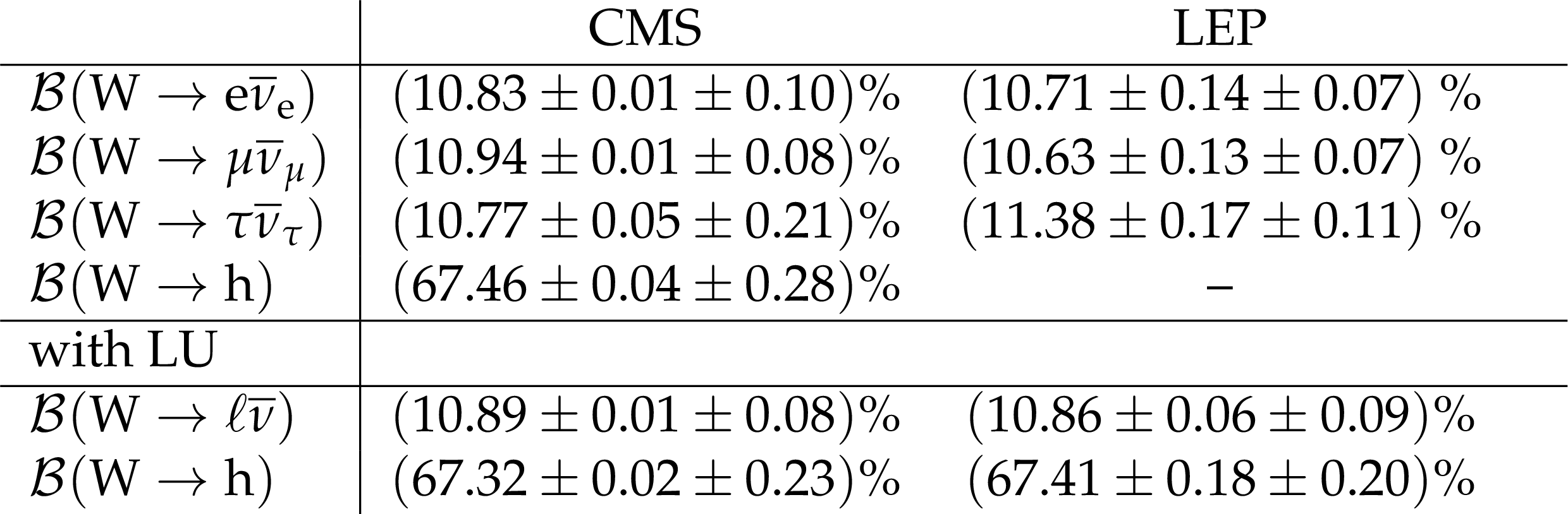
Table 3:
Values of the W branching fractions determined here, compared to the corresponding LEP measurements. The bottom rows list the leptonic W branching fraction derived combining the three individual decay modes assuming lepton universality. Statistical and systematics uncertainties are quoted for each branching fraction. |
png pdf |
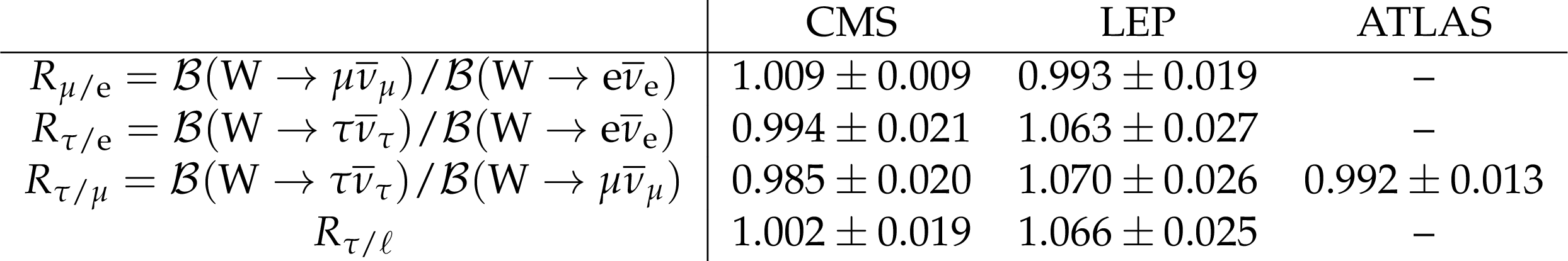
Table 4:
Ratios of different leptonic branching fractions measured in this analysis, and compared to the corresponding LEP and ATLAS results. |
| Summary |
|
Precise measurements of the three leptonic decay branching fractions of the W boson, as well as of the inclusive leptonic and hadronic ones assuming lepton universality, have been presented. The analysis is based on a data sample of proton-proton collisions at a center-of-mass energy of 13 TeV corresponding to an integrated luminosity of 35.9 fb$^{-1}$ recorded by the CMS experiment during the 2016 run. Events are collected online using single charged lepton triggers that require at least one prompt electron or muon with large transverse momentum. The offline analysis defines categories of final states consistent with the production of two W bosons, or a W boson plus jets, that decay leptonically. The extraction of W boson leptonic branching fractions is carried out through a binned maximum likelihood fit of multiple event categories, where the selected leptonic final states are further classified according to the number of jets as well as of the number of those jets identified as originating from bottom quarks, and binned by channel-dependent kinematic information. The branching fractions for the decay of the W boson into electrons, muons, taus, and hadrons are determined to be (10.83 $\pm$ 0.10 )%, (10.94 $\pm$ 0.08 )%, (10.77 $\pm$ 0.21 )%, and (67.46 $\pm$ 0.28 )%, respectively. These results are consistent with the lepton universality hypothesis of the standard model (SM) of particle physics, with a precision that exceeds that achieved by previous measurements based on data collected by the LEP experiments. When imposing lepton universality while fitting the data, values of (10.89 $\pm$ 0.08 )% and (67.32 $\pm$ 0.23 )% are obtained for the inclusive leptonic and hadronic branching fractions, respectively. From the ratio of inclusive hadronic-to-leptonic branching fractions compared to the corresponding theoretical prediction, further SM quantities can be derived. First, the square sum of the elements of the first two rows of the Cabibbo-Kobayashi-Maskawa (CKM) matrix are found to be $\sum_\mathrm{ij}|{\mathrm{V_{ij}}}|^{2} = $ 1.989 $\pm$ 0.021, thereby providing a precise test of CKM unitarity. The $|{\mathrm{V_{cs}}}|$ quark flavor mixing element can be fit similarly, finding $|{\mathrm{V_{cs}}}| = $ 0.969 $\pm$ 0.011, which is as precise as the current world-average of $|{\mathrm{V_{cs}}}| = $ 0.987 $\pm$ 0.011 obtained from direct D meson decays measurements. Finally, a value of the strong coupling constant at the W mass scale is obtained, ${\alpha_S}(m^{2}_\mathrm{W}) = $ 0.094 $\pm$ 0.033, that, although not competitive compared to the current world average value, confirms the usefulness of the W boson decays to constrain this fundamental SM parameter at future colliders. |
| Additional Figures | |
png pdf |
Additional Figure 1:
Summary of measured values of leptonic branching fractions from this measurement, LEP, and the combination of the two results. |
png pdf |
Additional Figure 2:
Two dimensional comparisons of leptonic branching fractions. For each pair shown in the panels, the branching fraction that is not shown has been marginalized over. The dashed lines correspond to 68% and 95% contour levels for the resulting two dimensional Gaussian distribution. |
png pdf |
Additional Figure 3:
Two dimensional distributions of the ratios $B({\mathrm {W}}\to \tau \nu)/B({\mathrm {W}}\to \mathrm{e}/\nu)$ vs $B({\mathrm {W}}\to \tau \nu)/B({\mathrm {W}}\to \mu \nu)$ with comparisons of the CMS, LEP, the combination of CMS and LEP, and ATLAS measurements. |
png |
Additional Figure 4:
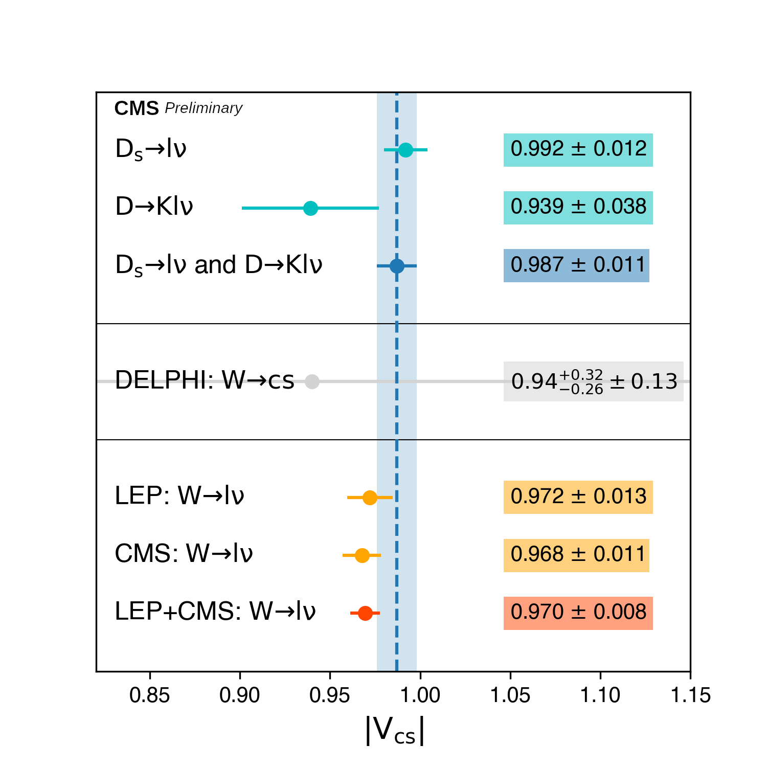
Measurements of $V_{\mathrm{cs}}$ from direct measurement using $\mathrm{D_{s}}^{+}\to {\mu} ^{+} {\nu} $, $\mathrm{D}\to \mathrm{K}\ell {\nu} $, and $ {\mathrm {W}}\to \mathrm{cs}$ decays compared to indirect measurements using $\mathcal {B}({\mathrm {W}}\to h)$ estimations. |
| Additional Tables | |
png pdf |
Additional Table 1:
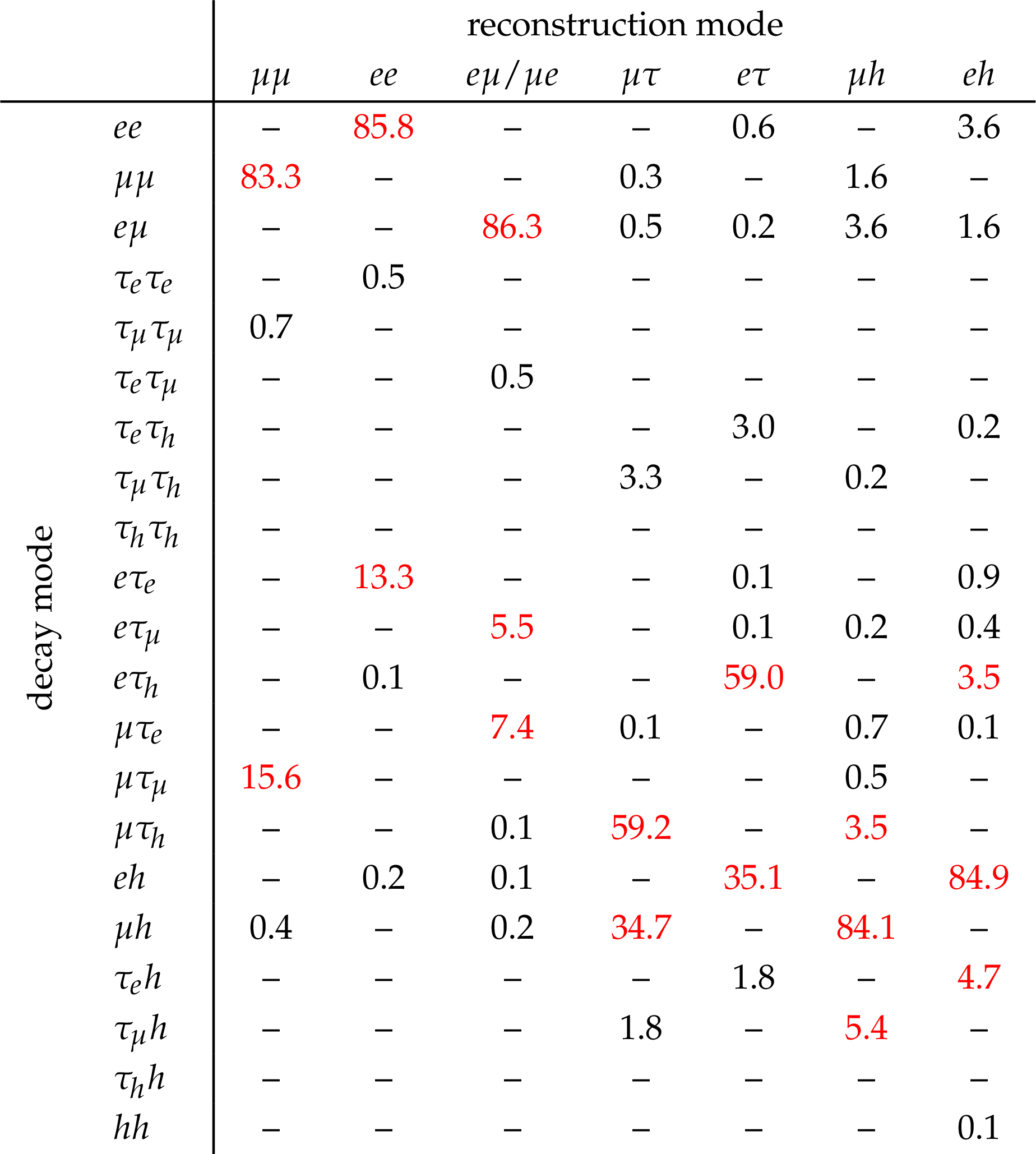
Percent of reconstructed final states attributable to different WW Figure decay modes. The quantities are estimated from simulated ${{\mathrm {t}\overline {\mathrm {t}}}}$ events where there are at least two jets and at least two b tags. The more significant contributions are highlighted in red. The statistical uncertainty on these quantities is negligible. |
png pdf |
Additional Table 2:
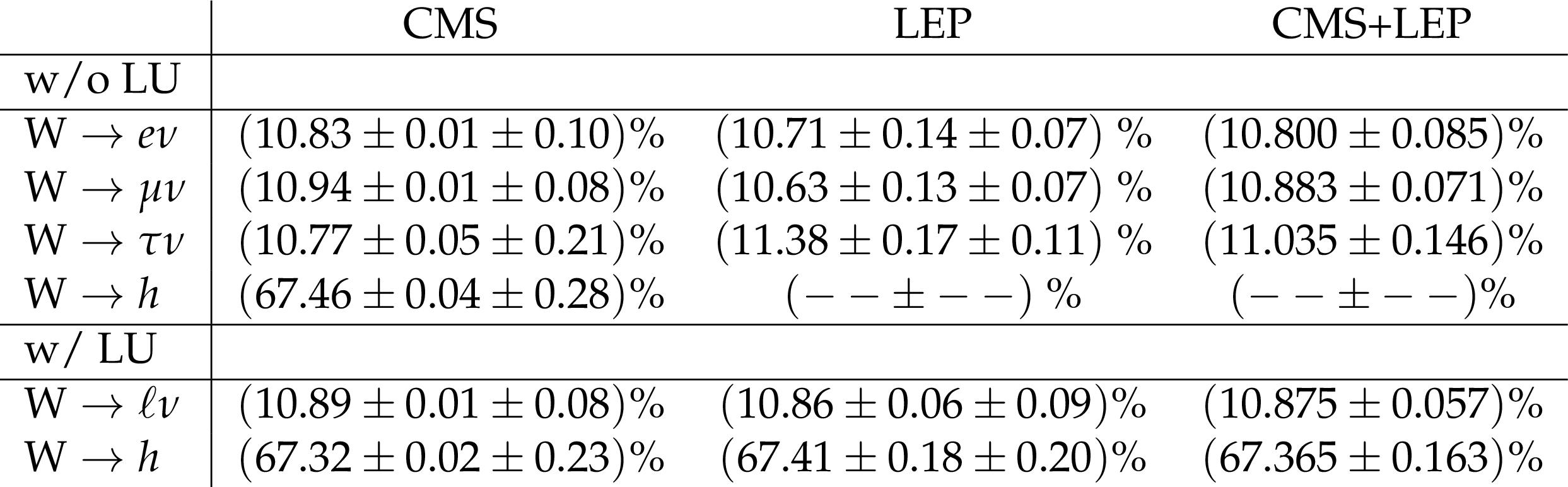
Values of branching fractions from this measurement, the combined LEP measurement, and both measurements combined assuming no correlation between experiments. The quoted uncertainties combine statistical and systematics sources. The combined values are calculated taking into account the correlations of the branching fractions in the individual measurements, but assuming no correlations between the uncertainties on the LEP and CMS measurements. The branching fractions are estimated in both scenario where lepton universality (LU) is required and when each of the leptonic branching fractions is free to take on an independent value. |
png pdf |
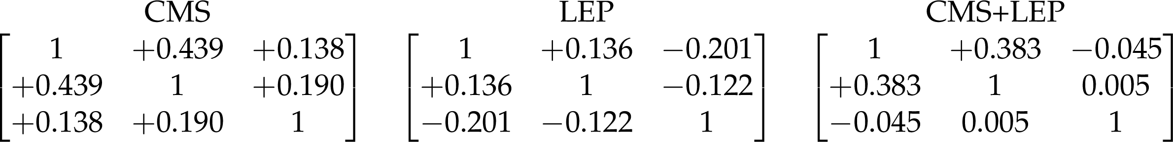
Additional Table 3:
Correlation matrices for leptonic branching fractions for both the CMS and LEP analyses. |
png pdf |
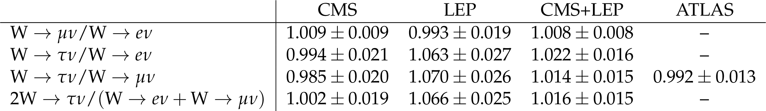
Additional Table 4:
Comparison of ratios of branching fractions measured by CMS, LEP, and ATLAS. Also included is the ratios of branching fractions after combining the measurement from both CMS and LEP. |
png pdf |
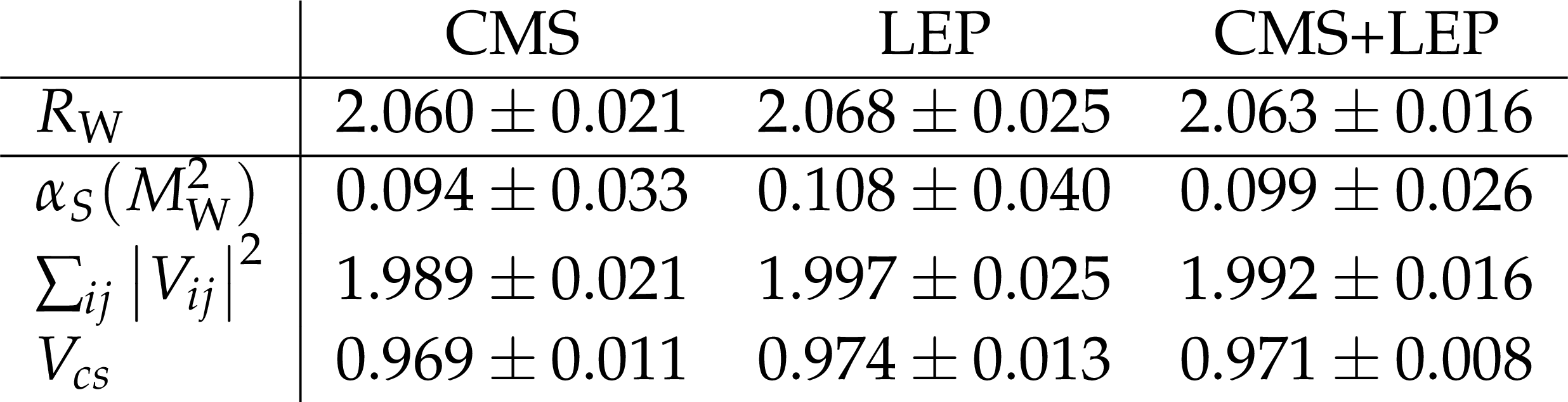
Additional Table 5:
The CMS and LEP results are combined assuming no correlations in the systematic uncertainties. The LEP value has been updated to account for updated values of $\alpha _{S}$ and the CKM matrix elements with respect to their originial reporting. |
| References | ||||
| 1 | W. Altmannshofer, P. Stangl, and D. M. Straub | Interpreting hints for lepton flavor universality violation | PRD 96 (2017) 055008 | 1704.05435 |
| 2 | LHCb Collaboration | Search for lepton-universality violation in $ B^+\to K^+\ell^+\ell^- $ decays | PRL 122 (2019) 191801 | 1903.09252 |
| 3 | DELPHI, OPAL, LEP Electroweak, ALEPH, L3 Collaboration | Electroweak measurements in electron-positron collisions at W-boson-pair energies at LEP | PR 532 (2013) 119 | 1302.3415 |
| 4 | A. Denner | Techniques for calculation of electroweak radiative corrections at the one loop level and results for W physics at LEP-200 | Fortsch. Phys. 41 (1993) 307 | 0709.1075 |
| 5 | B. A. Kniehl, F. Madricardo, and M. Steinhauser | Gauge independent W boson partial decay widths | PRD 62 (2000) 073010 | hep-ph/0005060 |
| 6 | D. d'Enterria and V. Jacobsen | Improved strong coupling determinations from hadronic decays of electroweak bosons at N$ ^3 $LO accuracy | (5, 2020) | 2005.04545 |
| 7 | ATLAS Collaboration | Test of the universality of $ \tau $ and $ \mu $ lepton couplings in W-boson decays from $ t\bar{t} $ events with the ATLAS detector | (7, 2020) | 2007.14040 |
| 8 | P. A. Baikov, K. G. Chetyrkin, and J. H. Kuhn | Order $ \alpha_s^4 $ QCD corrections to Z and tau decays | PRL 101 (2008) 012002 | 0801.1821 |
| 9 | D. Kara | Corrections of order $ \alpha \alpha_s $ to W boson decays | NPB 877 (2013) 683 | 1307.7190 |
| 10 | D. d'Enterria and M. Srebre | $ \alpha_s $ and $ \rm V_{cs} $ determination, and CKM unitarity test, from W decays at NNLO | PLB 763 (2016) 465 | 1603.06501 |
| 11 | Particle Data Group, P. A. Zyla et al. | Review of particle physics | Prog. Theor. Exp. Phys. 2020 (2020) 083C01 | |
| 12 | CMS Collaboration | The CMS experiment at the CERN LHC | JINST 3 (2008) S08004 | CMS-00-001 |
| 13 | S. Alioli, P. Nason, C. Oleari, and E. Re | A general framework for implementing NLO calculations in shower Monte Carlo programs: the POWHEG BOX | JHEP 06 (2010) 043 | 1002.2581 |
| 14 | A. Kardos, P. Nason, and C. Oleari | Three-jet production in POWHEG | JHEP 04 (2014) 043 | 1402.4001 |
| 15 | S. Frixione and B. R. Webber | Matching NLO QCD computations and parton shower simulations | JHEP 06 (2002) 029 | hep-ph/0204244 |
| 16 | P. Nason | A new method for combining NLO QCD with shower Monte Carlo algorithm | JHEP 11 (2004) 040 | hep-ph/0409146 |
| 17 | E. Re | Single-top Wt-channel production matched with parton showers using the POWHEG method | EPJC 71 (2011) 1547 | 1009.2450 |
| 18 | J. Alwall et al. | Madgraph 5: going beyond | Journal of High Energy Physics 2011 (Jun, 2011) | |
| 19 | J. Alwall et al. | The automated computation of tree-level and next-to-leading order differential cross sections, and their matching to parton shower simulations | JHEP 07 (2014) 079 | 1405.0301 |
| 20 | S. Frixione, P. Nason, and C. Oleari | Matching NLO QCD computations with parton shower simulations: the POWHEG method | JHEP 11 (2007) 070 | 0709.2092 |
| 21 | T. Sjostrand et al. | An introduction to PYTHIA 8.2 | CPC 191 (2015) 159 | 1410.3012 |
| 22 | P. Skands, S. Carrazza, and J. Rojo | Tuning PYTHIA 8.1: the Monash 2013 tune | EPJC 74 (2014) 3024 | 1404.5630 |
| 23 | GEANT4 Collaboration | GEANT4--a simulation toolkit | NIMA 506 (2003) 250 | |
| 24 | CMS Collaboration | The CMS trigger system | JINST 12 (2017) P01020 | CMS-TRG-12-001 1609.02366 |
| 25 | CMS Collaboration | Particle-flow reconstruction and global event description with the CMS detector | JINST 12 (2017) P10003 | CMS-PRF-14-001 1706.04965 |
| 26 | CMS Collaboration | Description and performance of track and primary-vertex reconstruction with the CMS tracker | JINST 9 (2014) P10009 | CMS-TRK-11-001 1405.6569 |
| 27 | CMS Collaboration | Performance of CMS muon reconstruction in pp collision events at $ \sqrt{s}= $ 7 TeV | JINST 7 (2012) P10002 | CMS-MUO-10-004 1206.4071 |
| 28 | CMS Collaboration | Performance of the CMS muon detector and muon reconstruction with proton-proton collisions at $ \sqrt{s}= $ 13 TeV | JINST 13 (2018) P06015 | CMS-MUO-16-001 1804.04528 |
| 29 | S. Baffioni et al. | Electron reconstruction in CMS | EPJC 49 (2007) 1099 | |
| 30 | CMS Collaboration | Measurements of properties of the Higgs boson decaying into the four-lepton final state in pp collisions at $ \sqrt{s}= $ 13 TeV | JHEP 11 (2017) 047 | CMS-HIG-16-041 1706.09936 |
| 31 | CMS Collaboration | Performance of electron reconstruction and selection with the CMS detector in proton-proton collisions at $ \sqrt{s} = $ 8 TeV | JINST 10 (2015) P06005 | CMS-EGM-13-001 1502.02701 |
| 32 | CMS Collaboration | Electron and photon reconstruction and identification with the CMS experiment at the CERN LHC | CMS-EGM-17-001 2012.06888 |
|
| 33 | CMS Collaboration | Performance of reconstruction and identification of $ \tau $ leptons decaying to hadrons and $ \nu_\tau $ in pp collisions at $ \sqrt{s}= $ 13 TeV | JINST 13 (2018) P10005 | CMS-TAU-16-003 1809.02816 |
| 34 | M. Cacciari, G. P. Salam, and G. Soyez | The anti-$ {k_{\mathrm{T}}} $ jet clustering algorithm | JHEP 04 (2008) 063 | 0802.1189 |
| 35 | CMS Collaboration | Determination of jet energy calibration and transverse momentum resolution in CMS | JINST 6 (2011) 11002 | CMS-JME-10-011 1107.4277 |
| 36 | CMS Collaboration | Identification of heavy-flavour jets with the CMS detector in pp collisions at 13 TeV | JINST 13 (2018) P05011 | CMS-BTV-16-002 1712.07158 |
| 37 | B. Pollack, S. Bhattacharya, and M. Schmitt | Bayesian blocks in high energy physics: Better binning made easy! | 1708.00810 | |
| 38 | J. S. Conway | Incorporating nuisance parameters in likelihoods for multisource spectra | in Proceedings, PHYSTAT 2011 Workshop on Statistical Issues Related to Discovery Claims in Search Experiments and Unfolding, CERN 2011 | 1103.0354 |
| 39 | CMS Collaboration | CMS luminosity measurement for the 2016 data-taking period | CMS-PAS-LUM-15-001 | CMS-PAS-LUM-15-001 |
| 40 | CMS Collaboration | Measurement of the inelastic proton-proton cross section at $ \sqrt{s}= $ 13 TeV | JHEP 07 (2018) 161 | CMS-FSQ-15-005 1802.02613 |
| 41 | CMS Collaboration | Measurements of inclusive W and Z cross sections in pp collisions at $ \sqrt{s}= $ 7 TeV | JHEP 01 (2011) 080 | CMS-EWK-10-002 1012.2466 |
| 42 | CMS Collaboration | Investigations of the impact of the parton shower tuning in PYTHIA 8 in the modelling of $ \mathrm{t\overline{t}} $ at $ \sqrt{s}= $ 8 and 13 TeV | CMS-PAS-TOP-16-021 | CMS-PAS-TOP-16-021 |
| 43 | D. V. Hinkley | On the ratio of two correlated normal random variables | Biometrika 56 (1969) 635 | |
| 44 | FCC Collaboration | FCC-ee: The Lepton Collider: Future Circular Collider Conceptual Design Report Volume 2 | EPJST 228 (2019) 261 | |
|
|
Compact Muon Solenoid LHC, CERN |
|

|

|

|

|

|