CMS-PAS-HIG-17-028

CMS-PAS-HIG-17-028
Combined measurement and interpretation of differential Higgs boson production cross sections at $\sqrt{s}=$ 13 TeV
CMS Collaboration
July 2018

Abstract: The differential Higgs boson production cross sections are sensitive probes for new physics beyond the standard model. In particular, new physics may contribute in the gluon-gluon fusion loop, the dominant Higgs boson production mechanism at the LHC, and manifest itself as deviations from the expected standard model distributions. Combined spectra from the $\mathrm{H}\to\gamma\gamma$ , $\mathrm{H}\to \mathrm{ZZ}$ and $\mathrm{H}\to \mathrm{b\bar{b}}$ decay channels are presented, together with limits on the Higgs couplings using 35.9 fb $^{-1}$ of proton-proton collision data recorded with the CMS detector at $\sqrt{s}=$ 13 TeV.
Links: CDS record (PDF) ; CADI line (restricted) ; These preliminary results are superseded in this paper, PLB 792 (2019) 369. The superseded preliminary plots can be found here.

Figures & Tables	Summary	Additional Figures	References	CMS Publications

Figures
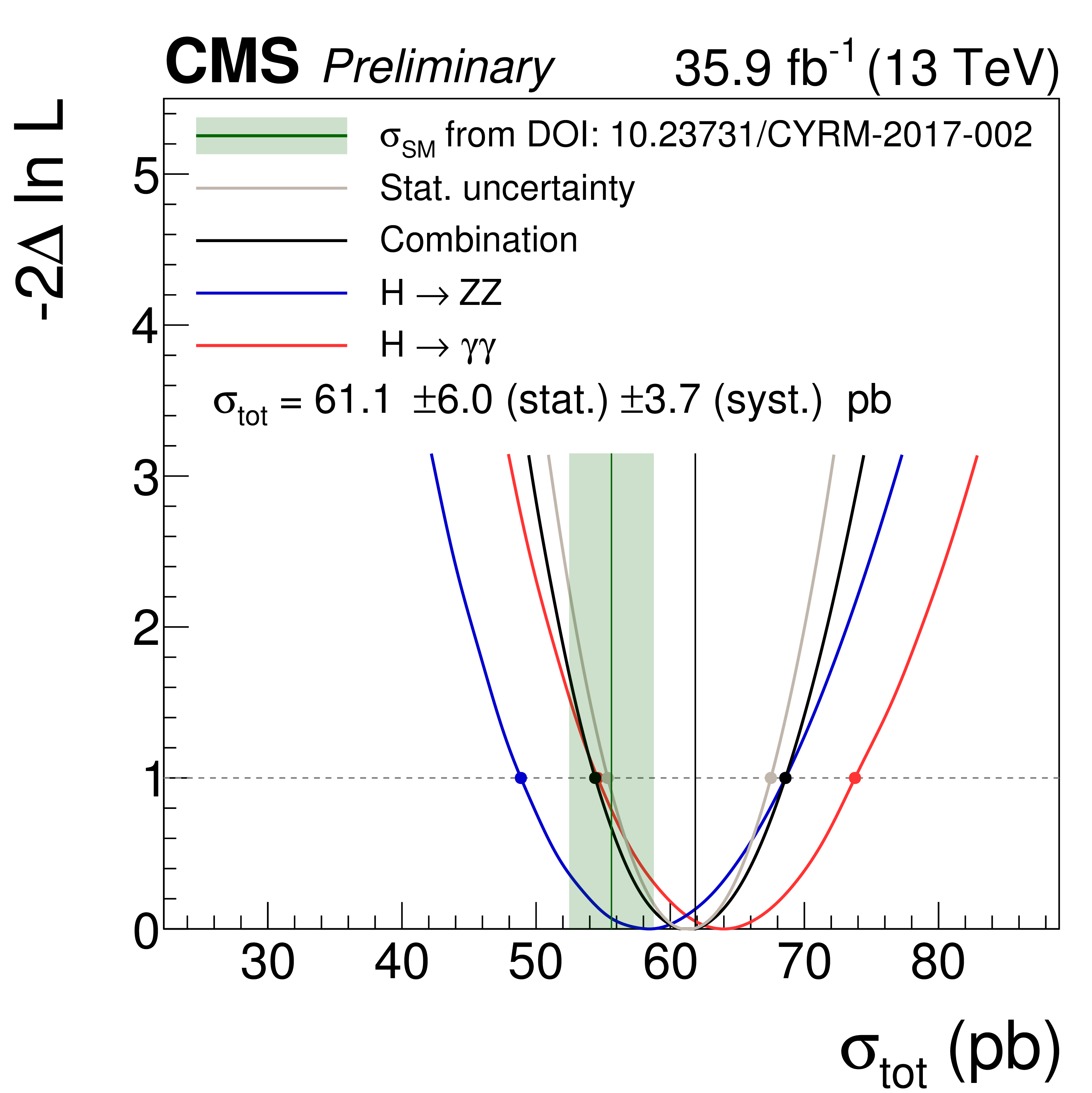
png pdf	Figure 1: (left) Scan of the total cross section $\sigma _\text {tot}$ , based on a combination of the total cross sections from $\mathrm{H} \to \gamma \gamma$ (64.0 $\pm$ 9.6 pb) and $\mathrm{H} \to \mathrm{ZZ}$ (58.2 $\pm$ 9.8 pb. (right) Scan of the ratio of branching fractions $R$ based on a combination of $\mathrm{H} \to \gamma \gamma$ and $\mathrm{H} \to \mathrm{ZZ}$ , while profiling all other parameters. The filled markers indicate the one standard deviation interval.
png pdf	Figure 1-a: Scan of the total cross section $\sigma _\text {tot}$ , based on a combination of the total cross sections from $\mathrm{H} \to \gamma \gamma$ (64.0 $\pm$ 9.6 pb) and $\mathrm{H} \to \mathrm{ZZ}$ (58.2 $\pm$ 9.8 pb. The filled markers indicate the one standard deviation interval.
png pdf	Figure 1-b: Scan of the ratio of branching fractions $R$ based on a combination of $\mathrm{H} \to \gamma \gamma$ and $\mathrm{H} \to \mathrm{ZZ}$ , while profiling all other parameters. The filled markers indicate the one standard deviation interval.
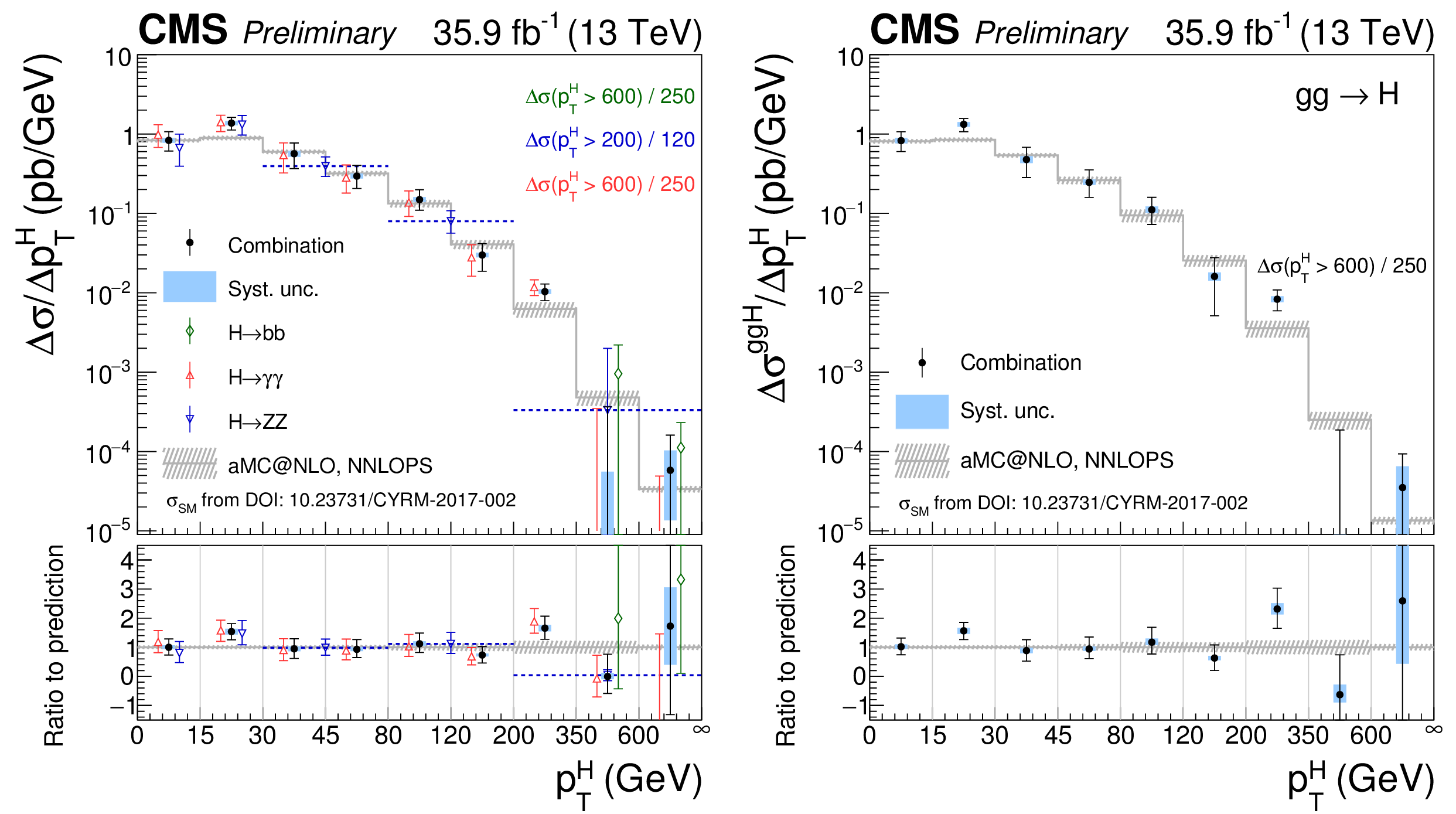
png pdf	Figure 2: Best fit values and uncertainties of the cross sections and signal strengths. (left) ${p_{\mathrm {T}}} ^{\text {H}}$ . (right) ${p_{\mathrm {T}}} ^{\text {H}}$ while fixing non-gluon-fusion contributions to their SM expectation.
png pdf	Figure 2-a: Best fit values and uncertainties of the cross sections and signal strengths: ${p_{\mathrm {T}}} ^{\text {H}}$ .
png pdf	Figure 2-b: Best fit values and uncertainties of the cross sections and signal strengths: ${p_{\mathrm {T}}} ^{\text {H}}$ while fixing non-gluon-fusion contributions to their SM expectation.
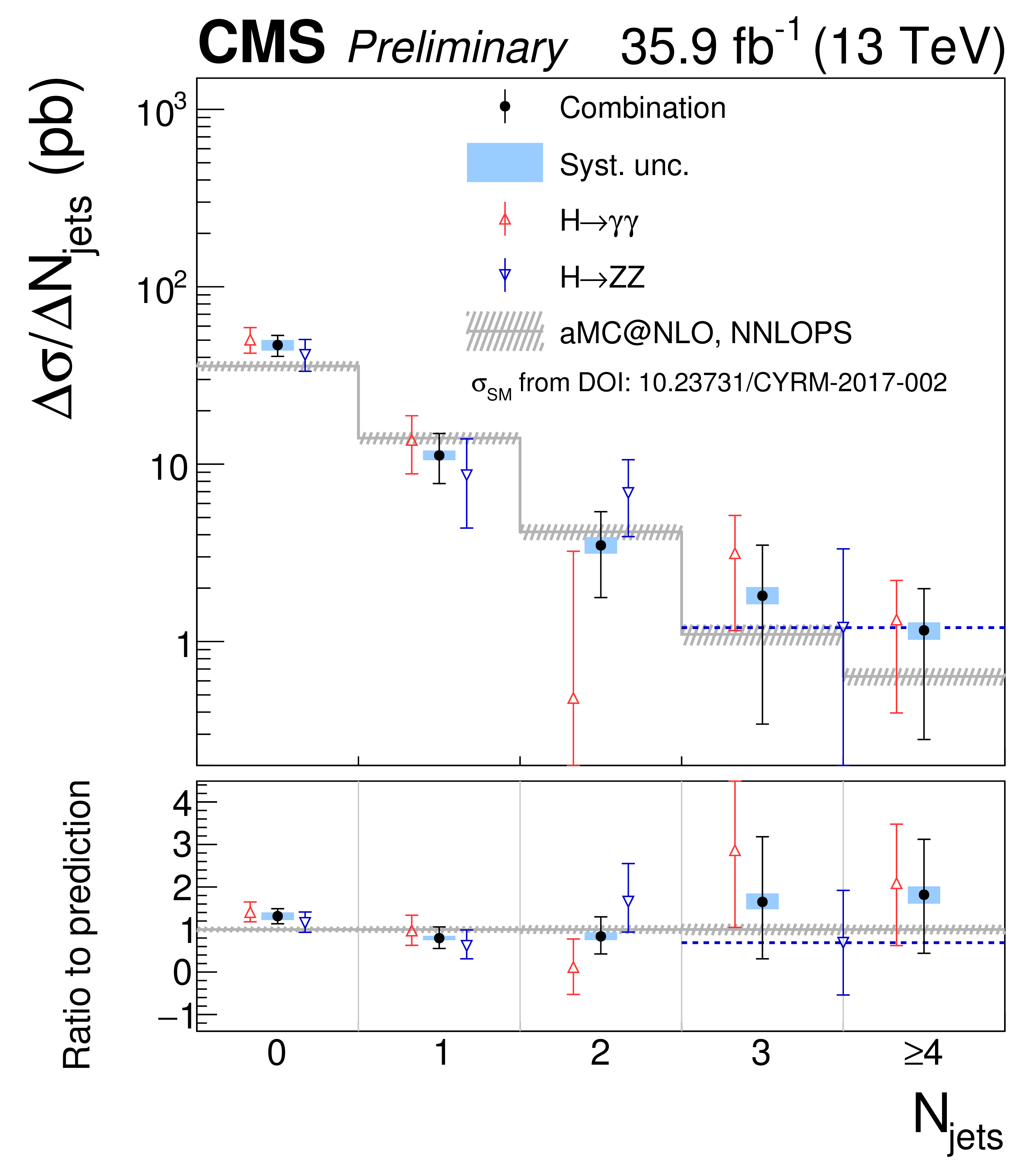
png pdf	Figure 3: Best fit values and uncertainties of the cross sections and signal strengths for the $N_\text {jets}$ -spectrum.
png pdf	Figure 4: Expected best fit values and uncertainties of the cross sections and signal strengths for the $\|y_{\text {H}} \|$ -spectrum.
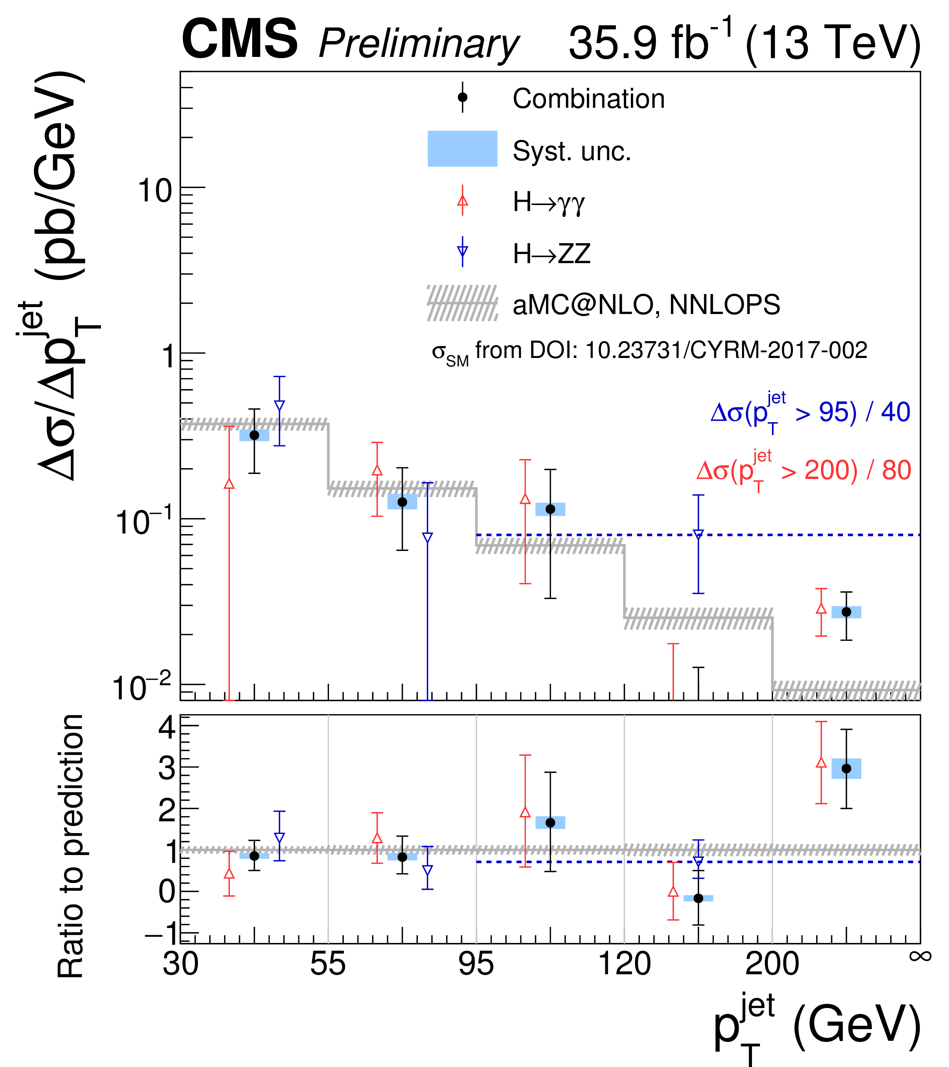
png pdf	Figure 5: Expected best fit values and uncertainties of the cross sections and signal strengths for the ${p_{\mathrm {T}}} ^\text {jet}$ -spectrum.
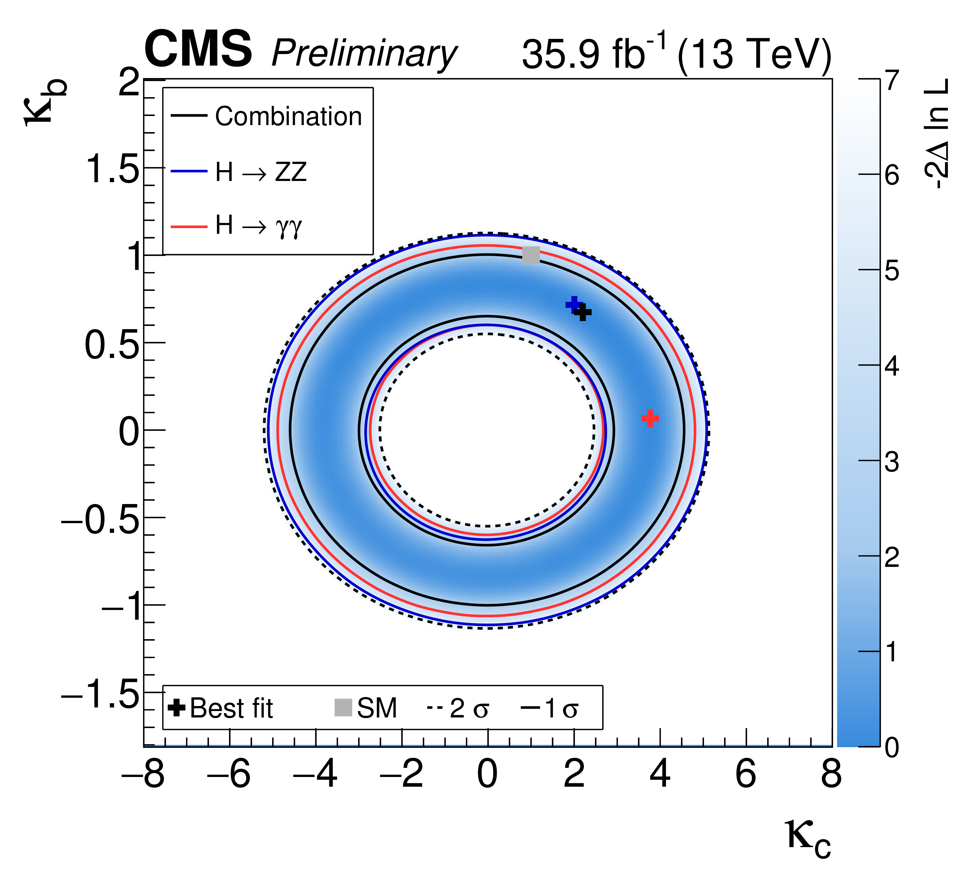
png pdf	Figure 6: Simultaneous fit results for $\kappa _b$ and $\kappa _c$ . (left) One and two standard deviation contours are shown for the combined ( $\mathrm{H} \to \gamma \gamma$ and $\mathrm{H} \to \mathrm{ZZ}$ ) fit to data and for $\mathrm{H} \to \gamma \gamma$ and $\mathrm{H} \to \mathrm{ZZ}$ separately, assuming a coupling dependency of the branching fractions. (right) One and two standard deviation contours are shown for the combined ( $\mathrm{H} \to \gamma \gamma$ and $\mathrm{H} \to \mathrm{ZZ}$ ) fit to data and for $\mathrm{H} \to \gamma \gamma$ and $\mathrm{H} \to \mathrm{ZZ}$ separately, assuming freely floating branching fractions.
png pdf	Figure 6-a: Simultaneous fit results for $\kappa _b$ and $\kappa _c$ . One and two standard deviation contours are shown for the combined ( $\mathrm{H} \to \gamma \gamma$ and $\mathrm{H} \to \mathrm{ZZ}$ ) fit to data and for $\mathrm{H} \to \gamma \gamma$ and $\mathrm{H} \to \mathrm{ZZ}$ separately, assuming a coupling dependency of the branching fractions.
png pdf	Figure 6-b: Simultaneous fit results for $\kappa _b$ and $\kappa _c$ . One and two standard deviation contours are shown for the combined ( $\mathrm{H} \to \gamma \gamma$ and $\mathrm{H} \to \mathrm{ZZ}$ ) fit to data and for $\mathrm{H} \to \gamma \gamma$ and $\mathrm{H} \to \mathrm{ZZ}$ separately, assuming freely floating branching fractions.
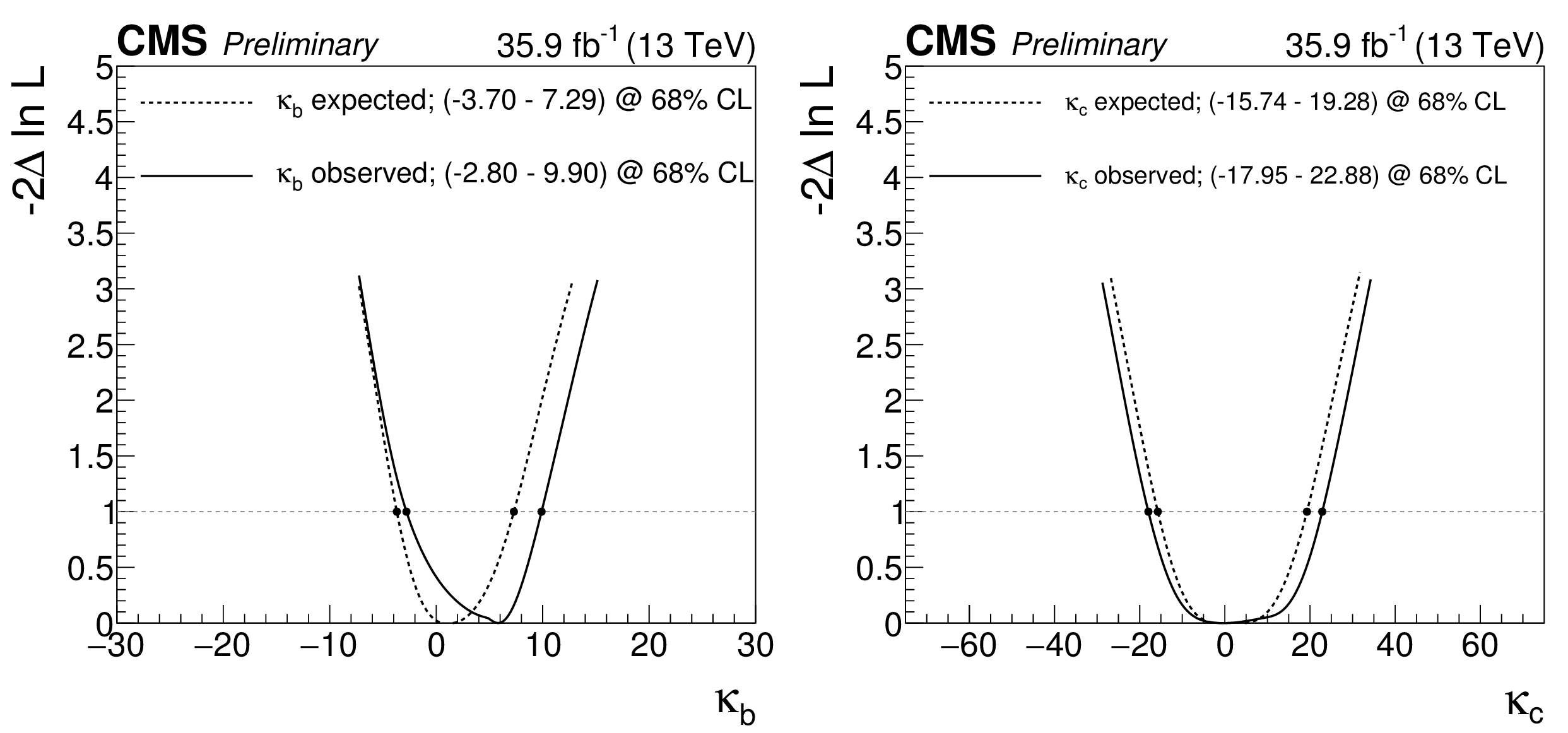
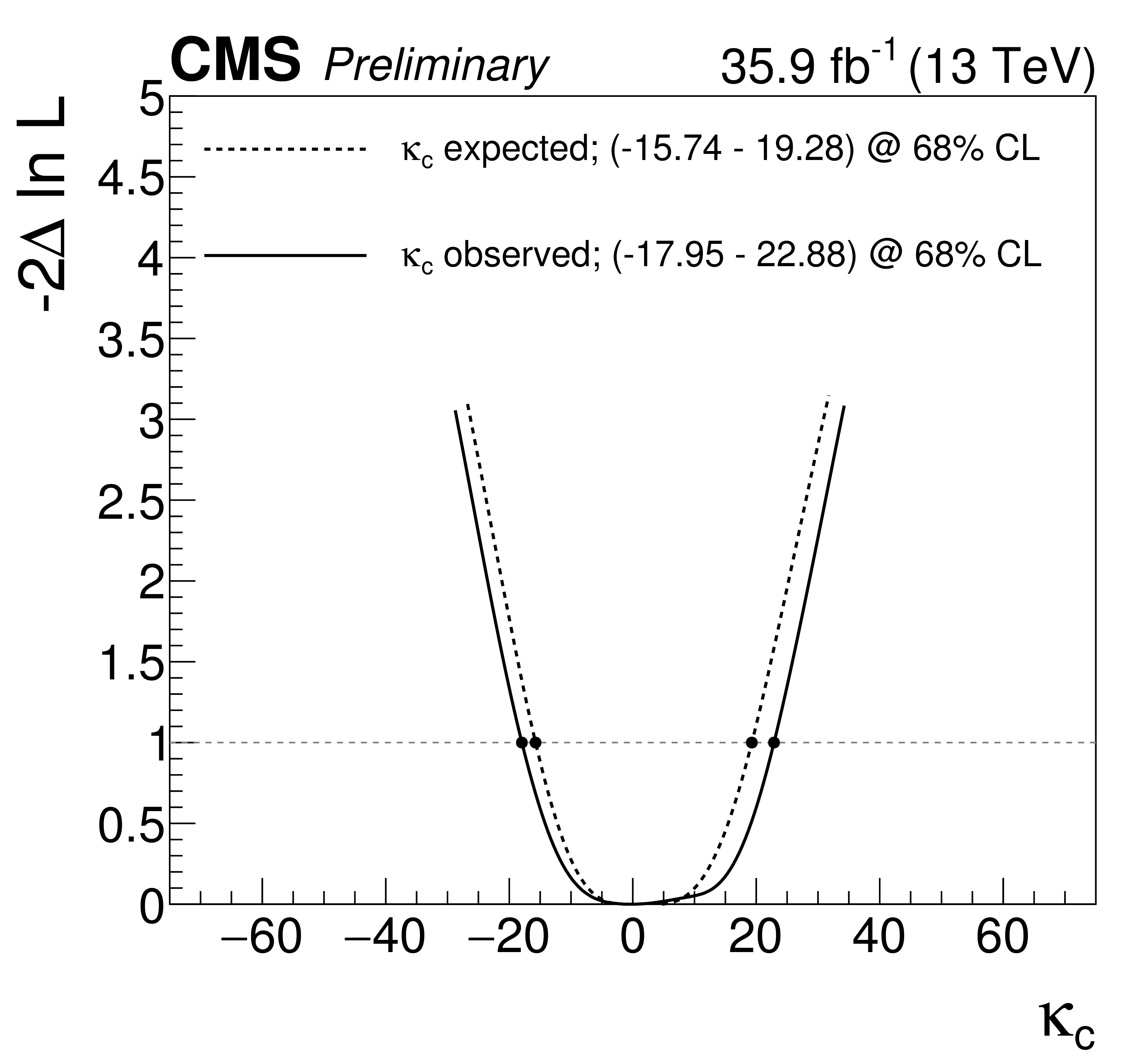
png pdf	Figure 7: Scans of only one coupling, while profiling the other. The filled markers indicate the one standard deviation interval. The branching fractions were considered dependent on the values of the couplings. (left) Scan of $\kappa _b$ while profiling $\kappa _c$ . (right) Scan of $\kappa _c$ while profiling $\kappa _b$ .
png pdf	Figure 7-a: Scan of $\kappa _b$ while profiling $\kappa _c$ . The filled markers indicate the one standard deviation interval. The branching fractions were considered dependent on the values of the couplings.
png pdf	Figure 7-b: Scan of $\kappa _c$ while profiling $\kappa _b$ . The filled markers indicate the one standard deviation interval. The branching fractions were considered dependent on the values of the couplings.
png pdf	Figure 8: Scans of only one coupling, while profiling the other. The filled markers indicate the one standard deviation interval. The branching fractions were freely floated in the fit. (left) Scan of $\kappa _b$ while profiling $\kappa _c$ . (right) Scan of $\kappa _c$ while profiling $\kappa _b$ .
png pdf	Figure 8-a: Scan of $\kappa _b$ while profiling $\kappa _c$ . The filled markers indicate the one standard deviation interval. The branching fractions were freely floated in the fit.
png pdf	Figure 8-b: Scan of $\kappa _c$ while profiling $\kappa _b$ . The filled markers indicate the one standard deviation interval. The branching fractions were freely floated in the fit.
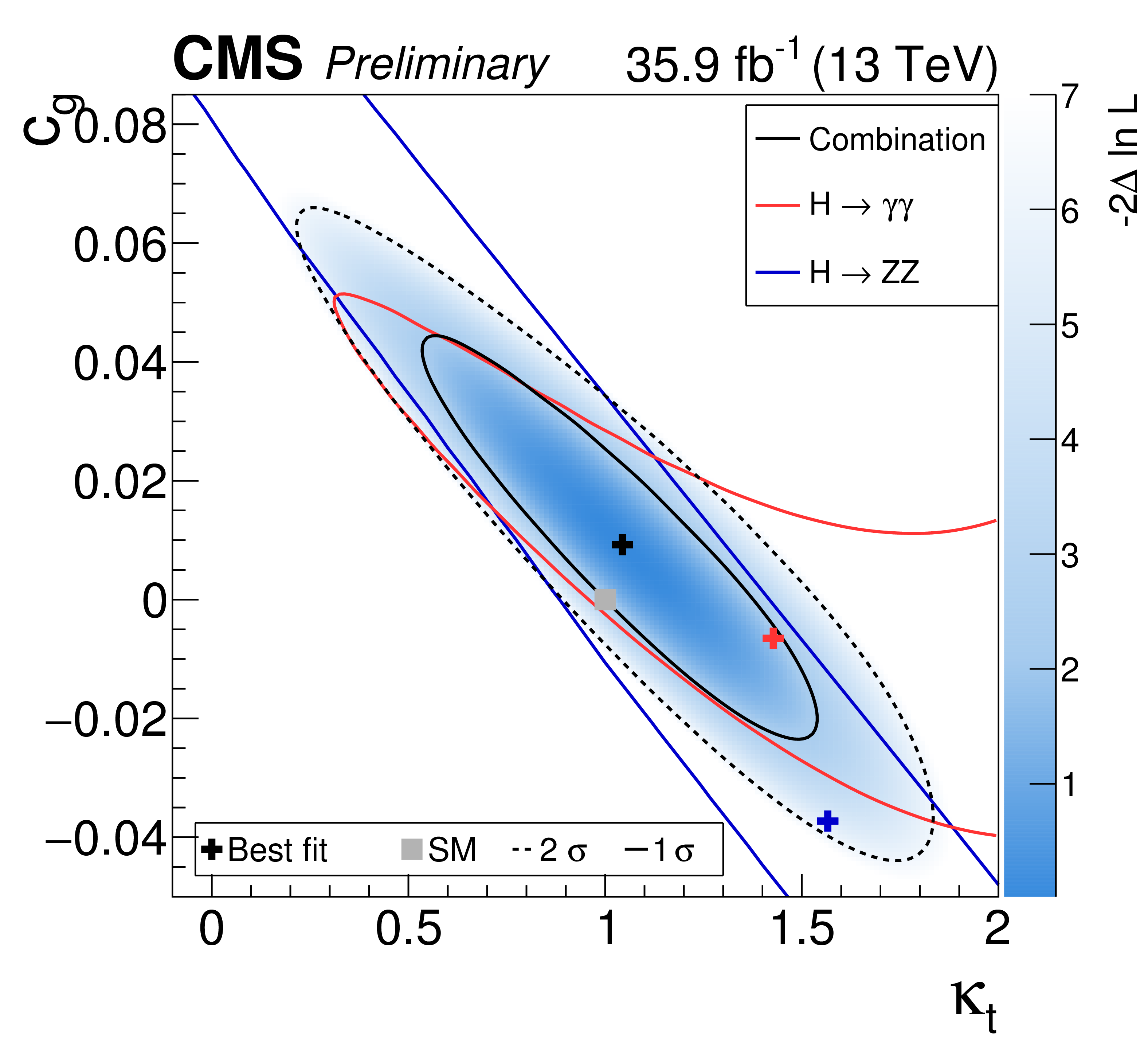
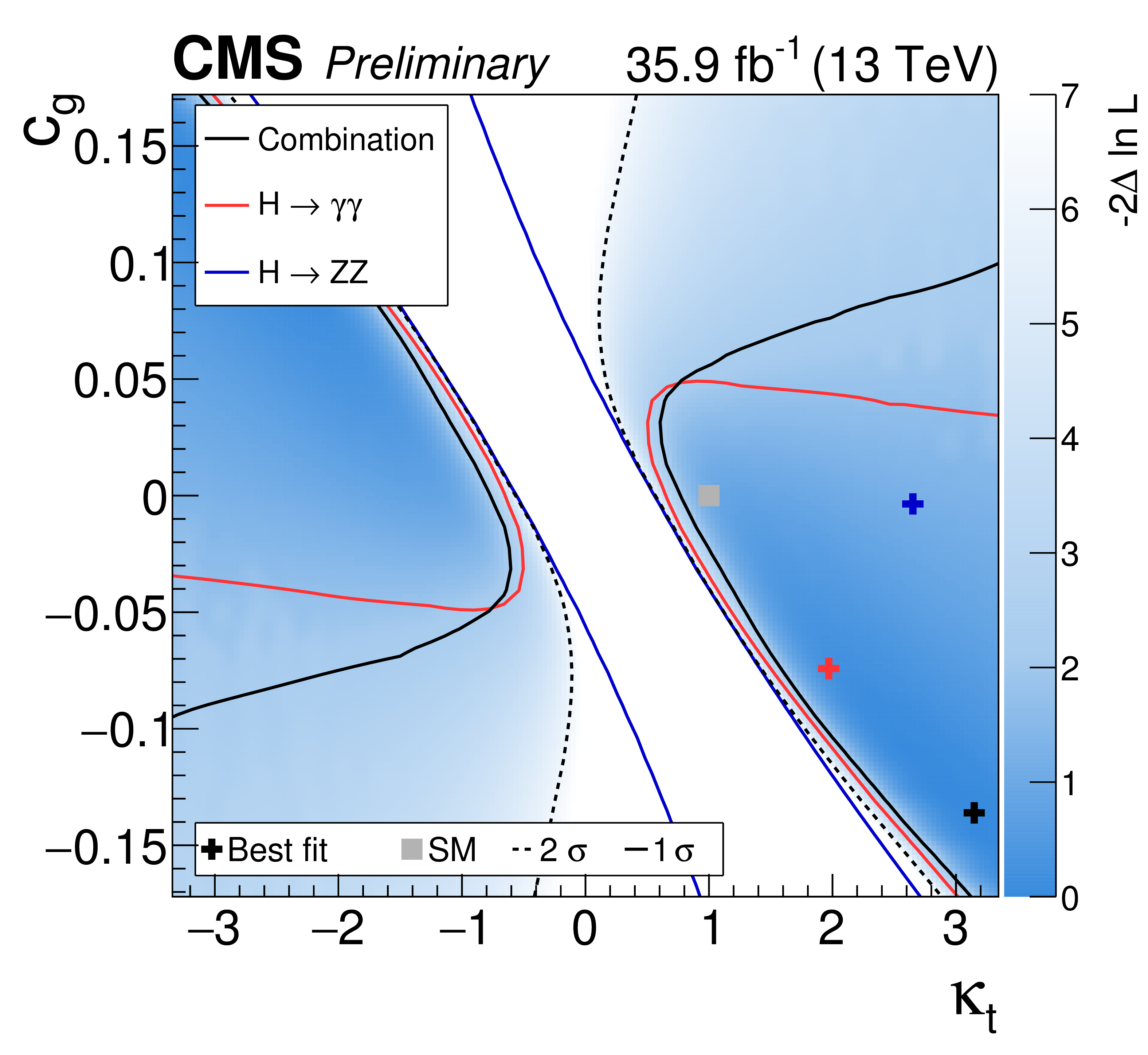
png pdf	Figure 9: Simultaneous fit results for $\kappa _t$ and $c_g$ . (left) One and two standard deviation contours are shown for the combined ( $\mathrm{H} \to \gamma \gamma$ , $\mathrm{H} \to \mathrm{ZZ}$ and $\mathrm{H} \to \mathrm{ b \bar{b} }$ ) fit to data and for $\mathrm{H} \to \gamma \gamma$ and $\mathrm{H} \to \mathrm{ZZ}$ separately, assuming a coupling dependency of the branching fractions. (right) One and two standard deviation contours are shown for the combined ( $\mathrm{H} \to \gamma \gamma$ , $\mathrm{H} \to \mathrm{ZZ}$ and $\mathrm{H} \to \mathrm{ b \bar{b} }$ ) fit to data and for $\mathrm{H} \to \gamma \gamma$ and $\mathrm{H} \to \mathrm{ZZ}$ separately, assuming freely floating branching fractions.
png pdf	Figure 9-a: One and two standard deviation contours are shown for the combined ( $\mathrm{H} \to \gamma \gamma$ , $\mathrm{H} \to \mathrm{ZZ}$ and $\mathrm{H} \to \mathrm{ b \bar{b} }$ ) fit to data and for $\mathrm{H} \to \gamma \gamma$ and $\mathrm{H} \to \mathrm{ZZ}$ separately, assuming a coupling dependency of the branching fractions.
png pdf	Figure 9-b: One and two standard deviation contours are shown for the combined ( $\mathrm{H} \to \gamma \gamma$ , $\mathrm{H} \to \mathrm{ZZ}$ and $\mathrm{H} \to \mathrm{ b \bar{b} }$ ) fit to data and for $\mathrm{H} \to \gamma \gamma$ and $\mathrm{H} \to \mathrm{ZZ}$ separately, assuming freely floating branching fractions.
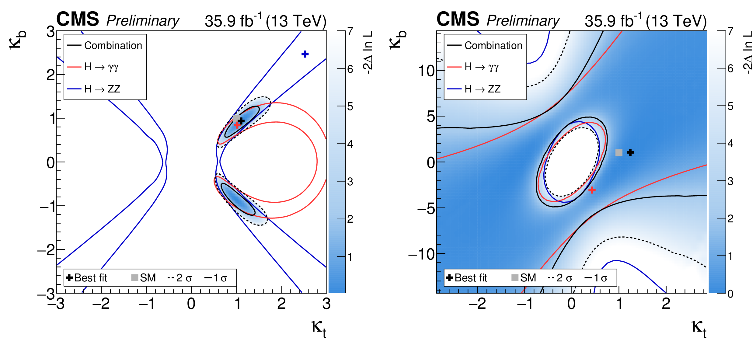
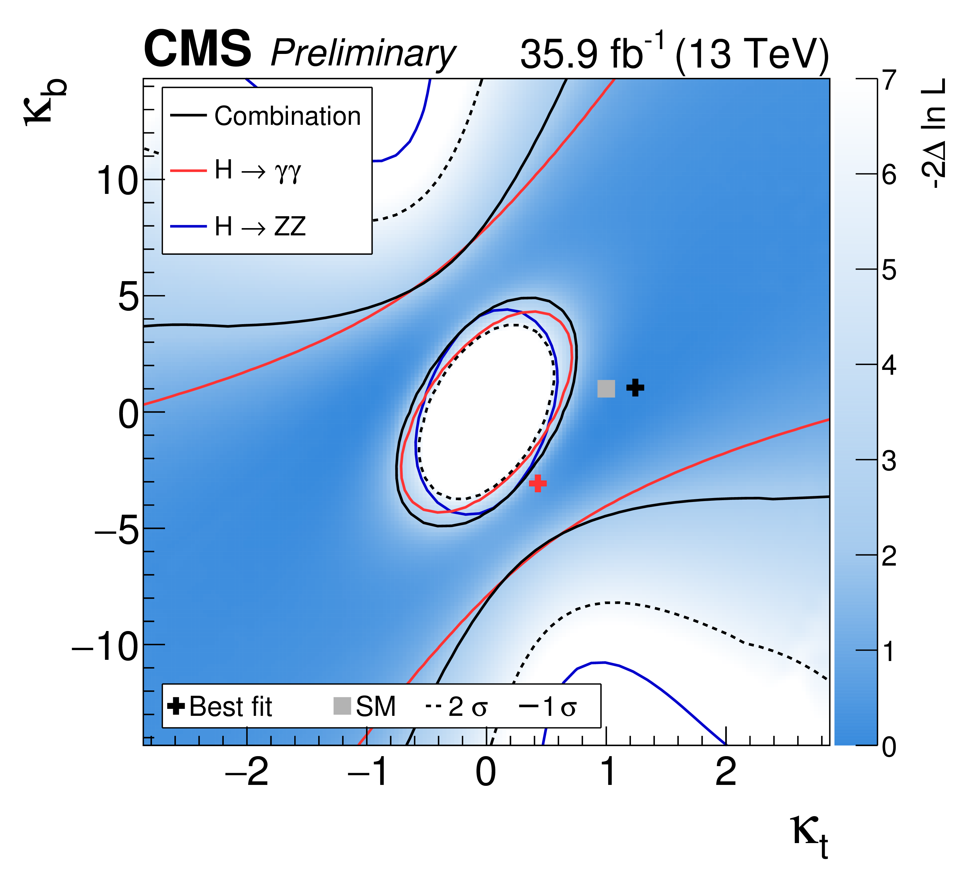
png pdf	Figure 10: Simultaneous combined fit results for $\kappa _t$ and $\kappa _b$ . (left) One and two standard deviation contours are shown for the combined ( $\mathrm{H} \to \gamma \gamma$ , $\mathrm{H} \to \mathrm{ZZ}$ and $\mathrm{H} \to \mathrm{ b \bar{b} }$ ) fit to data and for $\mathrm{H} \to \gamma \gamma$ and $\mathrm{H} \to \mathrm{ZZ}$ separately, assuming a coupling dependency of the branching fractions. (right) One and two standard deviation contours are shown for the combined ( $\mathrm{H} \to \gamma \gamma$ , $\mathrm{H} \to \mathrm{ZZ}$ and $\mathrm{H} \to \mathrm{ b \bar{b} }$ ) fit to data and for $\mathrm{H} \to \gamma \gamma$ and $\mathrm{H} \to \mathrm{ZZ}$ separately, where the branching fractions were freely floated in the fit.
png pdf	Figure 10-a: One and two standard deviation contours are shown for the combined ( $\mathrm{H} \to \gamma \gamma$ , $\mathrm{H} \to \mathrm{ZZ}$ and $\mathrm{H} \to \mathrm{ b \bar{b} }$ ) fit to data and for $\mathrm{H} \to \gamma \gamma$ and $\mathrm{H} \to \mathrm{ZZ}$ separately, assuming a coupling dependency of the branching fractions.
png pdf	Figure 10-b: One and two standard deviation contours are shown for the combined ( $\mathrm{H} \to \gamma \gamma$ , $\mathrm{H} \to \mathrm{ZZ}$ and $\mathrm{H} \to \mathrm{ b \bar{b} }$ ) fit to data and for $\mathrm{H} \to \gamma \gamma$ and $\mathrm{H} \to \mathrm{ZZ}$ separately, where the branching fractions were freely floated in the fit.
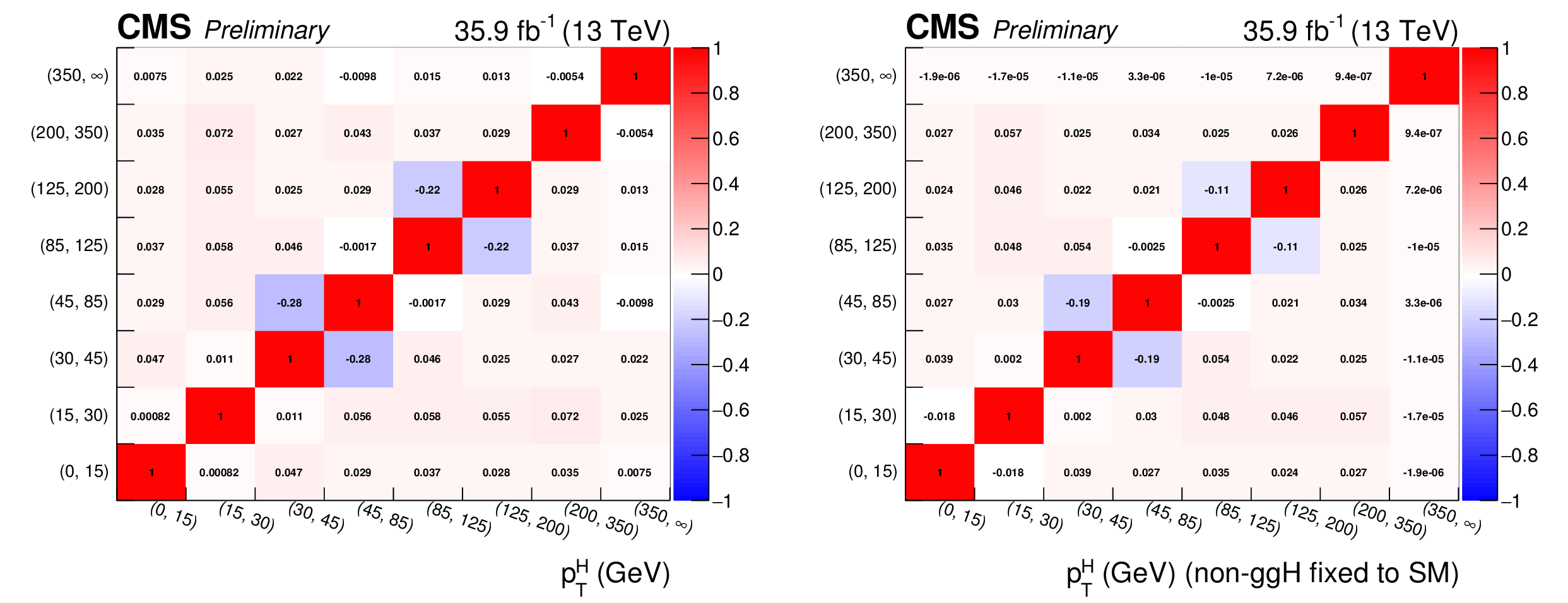
png pdf	Figure 11: (left) Bin-to-bin correlation matrix of the ${p_{\mathrm {T}}} ^{\text {H}}$ -spectrum. (right) Bin-to-bin correlation matrix of the ${p_{\mathrm {T}}} ^{\text {H}}$ -spectrum, while keeping the non-gluon-fusion contributions (xH) fixed to SM expectation.
png pdf	Figure 11-a: Bin-to-bin correlation matrix of the ${p_{\mathrm {T}}} ^{\text {H}}$ -spectrum.
png pdf	Figure 11-b: Bin-to-bin correlation matrix of the ${p_{\mathrm {T}}} ^{\text {H}}$ -spectrum, while keeping the non-gluon-fusion contributions (xH) fixed to SM expectation.
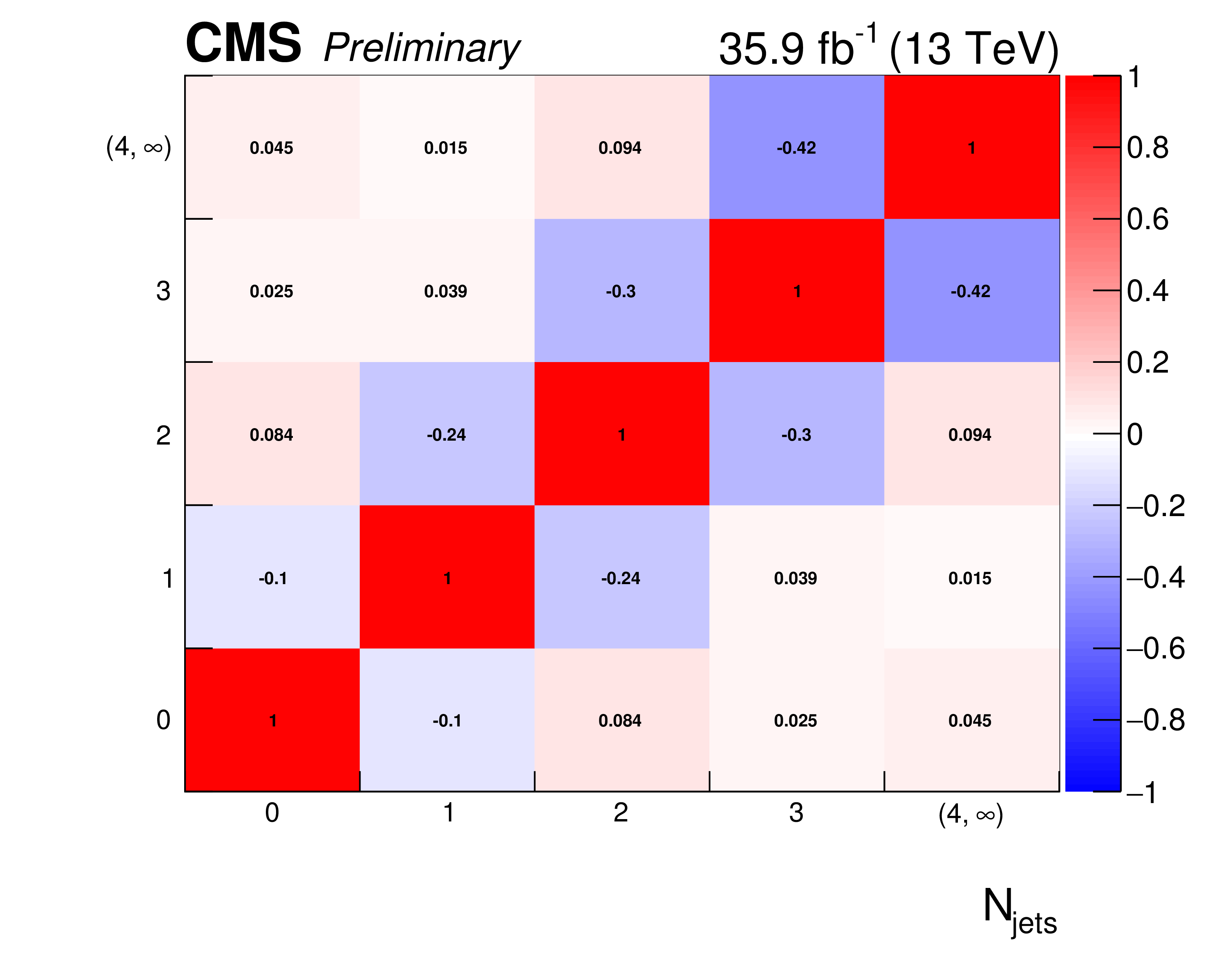
png pdf	Figure 12: Bin-to-bin correlation matrix of the $N_\text {jets}$ -spectrum.
png pdf	Figure 13: Bin-to-bin correlation matrix of the $\|y_{\text {H}} \|$ -spectrum.
png pdf	Figure 14: Bin-to-bin correlation matrix of the ${p_{\mathrm {T}}} ^\text {jet}$ -spectrum.

Tables
png pdf	Table 1: ${p_{\mathrm {T}}} ^{\text {H}}$ bin boundaries for the $\mathrm{H} \to \gamma \gamma$ , $\mathrm{H} \to \mathrm{ZZ}$ and $\mathrm{H} \to \mathrm{ b \bar{b} }$ decay channels.
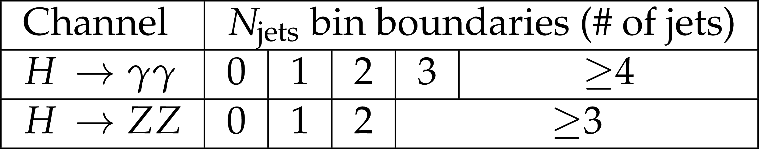
png pdf	Table 2: $N_\text {jets}$ bins for the $\mathrm{H} \to \gamma \gamma$ and the $\mathrm{H} \to \mathrm{ZZ}$ decay channels.
png pdf	Table 3: $\|y_{\text {H}} \|$ bins for the $\mathrm{H} \to \gamma \gamma$ and the $\mathrm{H} \to \mathrm{ZZ}$ decay channels.
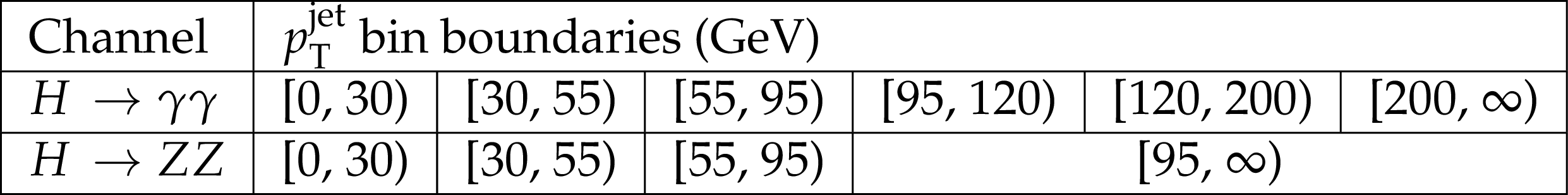
png pdf	Table 4: ${p_{\mathrm {T}}} ^\text {jet}$ bin boundaries for the $\mathrm{H} \to \gamma \gamma$ and the $\mathrm{H} \to \mathrm{ZZ}$ decay channels.
png pdf	Table 5: Theoretical uncertainties for the $\kappa _b$ / $\kappa _c$ spectra.
png pdf	Table 6: Theoretical uncertainties for the $\kappa _t$ / $c_g$ and $\kappa _t$ / $\kappa _b$ spectra.

Summary

A combination of differential cross sections for the differential observables

${p_{\mathrm{T}}}^{\text{H}}$ ,

$N_\text{jets}$ ,

$|y_\text{H} |$ and

${p_{\mathrm{T}}}^{\text{jet}}$ has been presented, using 35.9 fb

$^{-1}$ of proton-proton collision data obtained at

$\sqrt{s}=$ 13 TeV with the CMS detector. The spectra obtained are based on data from the

$\mathrm{H} \to\gamma\gamma$ ,

$\mathrm{H} \to \mathrm{ZZ}$ and

$\mathrm{H} \to \mathrm{b\bar{b}}$ decay channels. The overall uncertainty is decreased by 15% relative to that for

$\mathrm{H} \to\gamma\gamma$ alone by combining the

${p_{\mathrm{T}}}^{\text{H}}$ spectra. The decrease is larger in the lower

${p_{\mathrm{T}}}^{\text{H}}$ region than in the high

${p_{\mathrm{T}}}^{\text{H}}$ tails. No significant deviations from the SM are observed in any differential distribution.

The spectra obtained were interpreted in the Higgs coupling modifier framework, in which simultaneous variations of

$\kappa_b$ and

$\kappa_c$ ,

$\kappa_t$ and

$\kappa_g$ and

$\kappa_t$ and

$\kappa_b$ were fitted to the combination of the

${p_{\mathrm{T}}}^{\text{H}}$ -spectrum. The limits obtained on individual couplings were

$-0.9 < \kappa_b < 0.9$ and

$-4.3 < \kappa_c < 4.3$ , assuming the branching fractions scale with the coupling modifiers. For the charm coupling

$\kappa_c$ in particular, this measurement is competitive with those obtained from direct searches.

Additional Figures
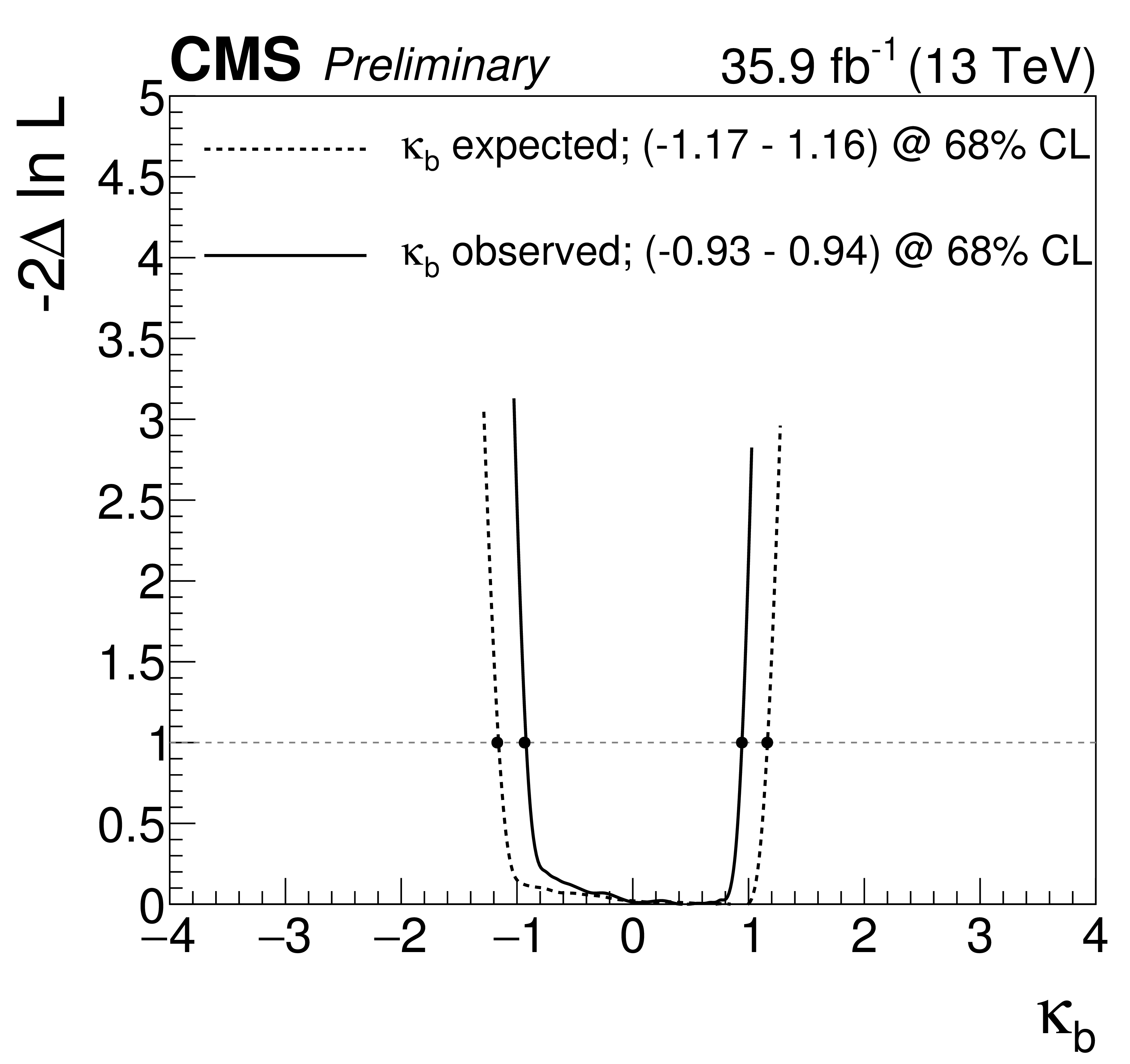
png pdf	Additional Figure 1: Simultaneous expected fit results for $\kappa _b$ and $\kappa _c$ . One and two standard deviation contours are shown for the combined ( $\mathrm{H} \rightarrow \gamma \gamma$ and $\mathrm{H} \rightarrow \mathrm{ZZ}$ ) expectation, fixing the branching fractions to the values expected from the standard model.
png pdf	Additional Figure 2: Expected fit of $\kappa _b$ while profiling $\kappa _c$ . The filled markers indicate the one standard deviation interval. The branching fractions were fixed to the values expected from the standard model.
png pdf	Additional Figure 3: Expected fit of $\kappa _c$ while profiling $\kappa _b$ . The filled markers indicate the one standard deviation interval. The branching fractions were fixed to the values expected from the standard model.

References
1	P. W. Higgs	Broken Symmetries and the Masses of Gauge Bosons	PRL 13 (1964) 508--509
2	F. Englert and R. Brout	Broken Symmetry and the Mass of Gauge Vector Mesons	PRL 13 (1964) 321--323
3	G. S. Guralnik, C. R. Hagen, and T. W. B. Kibble	Global Conservation Laws and Massless Particles	PRL 13 (1964) 585--587
4	ATLAS Collaboration	Observation of a new particle in the search for the Standard Model Higgs boson with the ATLAS detector at the LHC	PLB716 (2012) 1--29	1207.7214
5	CMS Collaboration	Observation of a new boson at a mass of 125 GeV with the CMS experiment at the LHC	PLB716 (2012) 30--61	CMS-HIG-12-028 1207.7235
6	ATLAS, CMS Collaboration	Measurements of the Higgs boson production and decay rates and constraints on its couplings from a combined ATLAS and CMS analysis of the LHC pp collision data at $\sqrt{s}=$ 7 and 8 TeV	JHEP 08 (2016) 045	1606.02266
7	ATLAS Collaboration	Measurements of the Higgs boson production and decay rates and coupling strengths using pp collision data at $\sqrt{s}=$ 7 and 8 TeV in the ATLAS experiment	EPJC76 (2016), no. 1, 6	1507.04548
8	CMS Collaboration	Precise determination of the mass of the Higgs boson and tests of compatibility of its couplings with the standard model predictions using proton collisions at 7 and 8 TeV	EPJC75 (2015), no. 5, 212	CMS-HIG-14-009 1412.8662
9	ATLAS Collaboration	Combined measurements of Higgs boson production and decay in the $H\rightarrow ZZ^*\rightarrow4\ell$ and $H\rightarrow\gamma\gamma$ channels using $\sqrt{s}=$ 13 TeV pp collision data collected with the ATLAS experiment	ATLAS Conference Note ATLAS-CONF-2017-047
10	CMS Collaboration	Combined measurements of the Higgs boson's couplings at $\sqrt{s}=$ 13 TeV	CMS-PAS-HIG-17-031	CMS-PAS-HIG-17-031
11	S. Dimopoulos and H. Georgi	Softly Broken Supersymmetry and SU(5)	NPB193 (1981) 150--162
12	E. Witten	Dynamical Breaking of Supersymmetry	NPB188 (1981) 513
13	F. Bishara, U. Haisch, P. F. Monni, and E. Re	Constraining Light-Quark Yukawa Couplings from Higgs Distributions	PRL 118 (2017), no. 12, 121801	1606.09253
14	ATLAS Collaboration	Measurements of the Total and Differential Higgs Boson Production Cross Sections Combining the $H\rightarrow\gamma\gamma$ and $H\rightarrow ZZ \rightarrow 4\ell$ Decay Channels at $\sqrt{s} =$ 8 TeV with the ATLAS Detector	PRL 115 (2015), no. 9, 091801	1504.05833
15	ATLAS Collaboration	Search for the Decay of the Higgs Boson to Charm Quarks with the ATLAS Experiment	PRL 120 (2018), no. 21, 211802	1802.04329
16	ATLAS Collaboration	Search for Higgs and Z Boson Decays to J/ $\psi\gamma$ and $\Upsilon(nS)\gamma$ with the ATLAS Detector	PRL 114 (2015), no. 12, 121801	1501.03276
17	M. Konig and M. Neubert	Exclusive Radiative Higgs Decays as Probes of Light-Quark Yukawa Couplings	JHEP 08 (2015) 012	1505.03870
18	LHCb Collaboration	Search for $H^0 \rightarrow b \bar{b}$ or $c \bar{c}$ in association with a $W$ or $Z$ boson in the forward region of $pp$ collisions	LHCb Conference Note LHCb-CONF-2016-006
19	I. Brivio, F. Goertz, and G. Isidori	Probing the Charm Quark Yukawa Coupling in Higgs+Charm Production	PRL 115 (2015), no. 21, 211801	1507.02916
20	ATLAS Collaboration	Measurements of fiducial and differential cross sections for Higgs boson production in the diphoton decay channel at $\sqrt{s}=$ 8 TeV with ATLAS	JHEP 09 (2014) 112	1407.4222
21	CMS Collaboration	Measurement of differential cross sections for Higgs boson production in the diphoton decay channel in pp collisions at $\sqrt{s}=$ 8 TeV	EPJC76 (2016), no. 1, 13	CMS-HIG-14-016 1508.07819
22	ATLAS Collaboration	Fiducial and differential cross sections of Higgs boson production measured in the four-lepton decay channel in $pp$ collisions at $\sqrt{s} =$ 8 TeV with the ATLAS detector	PLB738 (2014) 234--253	1408.3226
23	CMS Collaboration	Measurement of differential and integrated fiducial cross sections for Higgs boson production in the four-lepton decay channel in pp collisions at $\sqrt{s}=$ 7 and 8 TeV	JHEP 04 (2016) 005	CMS-HIG-14-028 1512.08377
24	ATLAS Collaboration	Measurement of fiducial differential cross sections of gluon-fusion production of Higgs bosons decaying to $WW^{*} \rightarrow e\nu\mu\nu$ with the ATLAS detector at $\sqrt{s}=$ 8 TeV	JHEP 08 (2016) 104	1604.02997
25	CMS Collaboration	Measurement of the transverse momentum spectrum of the Higgs boson produced in pp collisions at $\sqrt{s}=$ 8 TeV using $H \to WW$ decays	JHEP 03 (2017) 032	CMS-HIG-15-010 1606.01522
26	ATLAS Collaboration	Measurement of inclusive and differential cross sections in the $H \rightarrow ZZ^* \rightarrow 4\ell$ decay channel in $pp$ collisions at $\sqrt{s}=$ 13 TeV with the ATLAS detector	JHEP 10 (2017) 132	1708.02810
27	CMS Collaboration	Measurements of properties of the Higgs boson decaying into the four-lepton final state in pp collisions at $\sqrt{s}=$ 13 TeV	JHEP 11 (2017) 047	CMS-HIG-16-041 1706.09936
28	ATLAS Collaboration	Combined measurement of differential and total cross sections in the $H \rightarrow \gamma \gamma$ and the $H \rightarrow ZZ^* \rightarrow 4\ell$ decay channels at $\sqrt{s} =$ 13 TeV with the ATLAS detector	Submitted to PLB	1805.10197
29	ATLAS Collaboration	Measurements of Higgs boson properties in the diphoton decay channel with 36 fb $^{-1}$ of $pp$ collision data at $\sqrt{s} =$ 13 TeV with the ATLAS detector	Submitted to PRD	1802.04146
30	CMS Collaboration	Measurement of differential fiducial cross sections for Higgs boson production in the diphoton decay channel in pp collisions at $\sqrt{s}=$ 13 TeV	CMS-PAS-HIG-17-015	CMS-PAS-HIG-17-015
31	CMS Collaboration	Inclusive search for a highly boosted Higgs boson decaying to a bottom quark-antiquark pair	PRL 120 (2018), no. 7, 071802	CMS-HIG-17-010 1709.05543
32	LHC Higgs Cross Section Working Group Collaboration	LHC HXSWG interim recommendations to explore the coupling structure of a Higgs-like particle		1209.0040
33	CMS Collaboration	Performance of photon reconstruction and identification with the CMS detector in proton-proton collisions at $\sqrt{s} =$ 8 TeV	JINST 10 (2015) P08010	CMS-EGM-14-001 1502.02702
34	CMS Collaboration	The CMS experiment at the CERN LHC	JINST 3 (2008) S08004	CMS-00-001
35	J. Alwall et al.	The automated computation of tree-level and next-to-leading order differential cross sections, and their matching to parton shower simulations	JHEP 07 (2014) 079	1405.0301
36	T. Sjostrand et al.	An Introduction to PYTHIA 8.2	CPC 191 (2015) 159--177	1410.3012
37	P. Skands, S. Carrazza, and J. Rojo	Tuning PYTHIA 8.1: the Monash 2013 Tune	EPJC 74 (2014) 3024	1404.5630
38	K. Hamilton, P. Nason, and G. Zanderighi	MINLO: Multi-Scale Improved NLO	JHEP 10 (2012) 155	1206.3572
39	A. Kardos, P. Nason, and C. Oleari	Three-jet production in POWHEG	JHEP 04 (2014) 043	1402.4001
40	M. Dasgupta, A. Fregoso, S. Marzani, and G. P. Salam	Towards an understanding of jet substructure	JHEP 09 (2013) 029	1307.0007
41	A. J. Larkoski, S. Marzani, G. Soyez, and J. Thaler	Soft Drop	JHEP 05 (2014) 146	1402.2657
42	G. Cowan, K. Cranmer, E. Gross, and O. Vitells	Asymptotic formulae for likelihood-based tests of new physics	EPJC71 (2011) 1554	1007.1727
43	P. C. Hansen	The L-curve and its use in the numerical treatment of inverse problems	in Computational Inverse Problems in Electrocardiology, pp. 119--142 Southampton: WIT Press
44	M. Grazzini, A. Ilnicka, M. Spira, and M. Wiesemann	Effective Field Theory for Higgs properties parametrisation: the transverse momentum spectrum case	in 52nd Rencontres de Moriond on QCD and High Energy Interactions (Moriond QCD 2017) La Thuile, Italy, March 25-April 1, 2017 2017	1705.05143
45	A. Banfi, P. F. Monni, and G. Zanderighi	Quark masses in Higgs production with a jet veto	JHEP 01 (2014) 097	1308.4634
46	G. Bozzi, S. Catani, D. de Florian, and M. Grazzini	The q(T) spectrum of the Higgs boson at the LHC in QCD perturbation theory	PLB564 (2003) 65--72	hep-ph/0302104
47	T. Becher and M. Neubert	Drell-Yan Production at Small $q_T$ , Transverse Parton Distributions and the Collinear Anomaly	EPJC71 (2011) 1665	1007.4005
48	P. F. Monni, E. Re, and P. Torrielli	Higgs Transverse-Momentum Resummation in Direct Space	PRL 116 (2016), no. 24, 242001	1604.02191
49	LHC Higgs Cross Section Working Group Collaboration	Handbook of LHC Higgs Cross Sections: 4. Deciphering the Nature of the Higgs Sector		1610.07922