

Compact Muon Solenoid
LHC, CERN
| CMS-PAS-HIG-17-011 | ||
| Constraints on anomalous Higgs boson couplings in production and decay $\mathrm{ H }\to4\ell$ | ||
| CMS Collaboration | ||
| March 2017 | ||
| Abstract: The study of the anomalous interactions of the recently discovered Higgs boson is performed using the decay information $\mathrm{ H }\to 4\ell$ and information from associated production of two quark jets, originating either from vector boson fusion or associated vector boson. The full dataset recorded by the CMS experiment during 2016 of the LHC Run-2 is used, corresponding to an integrated luminosity of 35.9 fb$^{-1}$ at 13 TeV. Novel techniques are used for the study of associated VBF and VH production and its combination with analysis of decay information using optimal approaches based on matrix element techniques. The tensor structure of the interactions of the spin-zero Higgs boson with two vector bosons either in production or in decay is investigated and constraints are set on anomalous HVV interactions. All observations are consistent with the expectations for the standard model Higgs boson. | ||
|
Links:
CDS record (PDF) ;
CADI line (restricted) ;
These preliminary results are superseded in this paper, PLB 775 (2017) 1. The superseded preliminary plots can be found here. |
||
| Figures & Tables | Summary | Additional Figures | References | CMS Publications |
|---|
| Figures | |
png pdf |
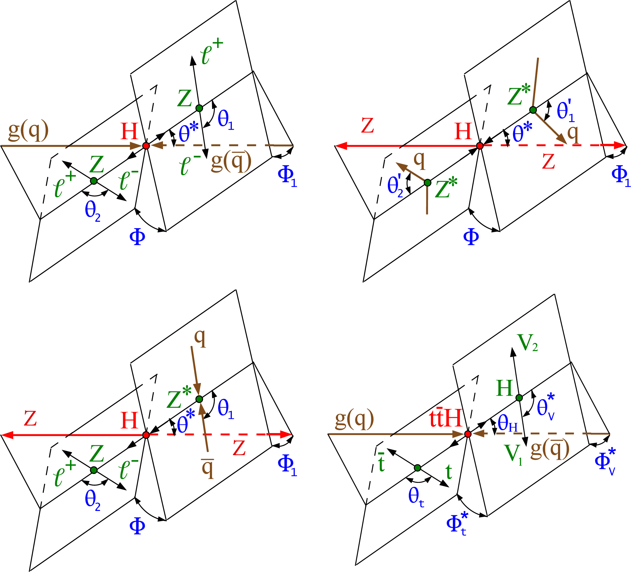
Figure 1:
Illustrations of H particle production and decay $gg/\mathrm{q\bar{q}}\to \mathrm{ H } \to ZZ\to 4\ell ^\pm $ (top-left), VBF $q{q^\prime }\to q{q^\prime } \mathrm{ H } $ (top-right), $\mathrm{q\bar{q}}\to V^*\to VH$ (bottom-left), and $\mathrm{gg}/\mathrm{q\bar{q}}\to t\bar{t} \mathrm{ H } $ (bottom-right). Angles and invariant masses fully characterize the orientation of the production and decay chain and are defined in the suitable rest frames [32,41,47]. |
png pdf |
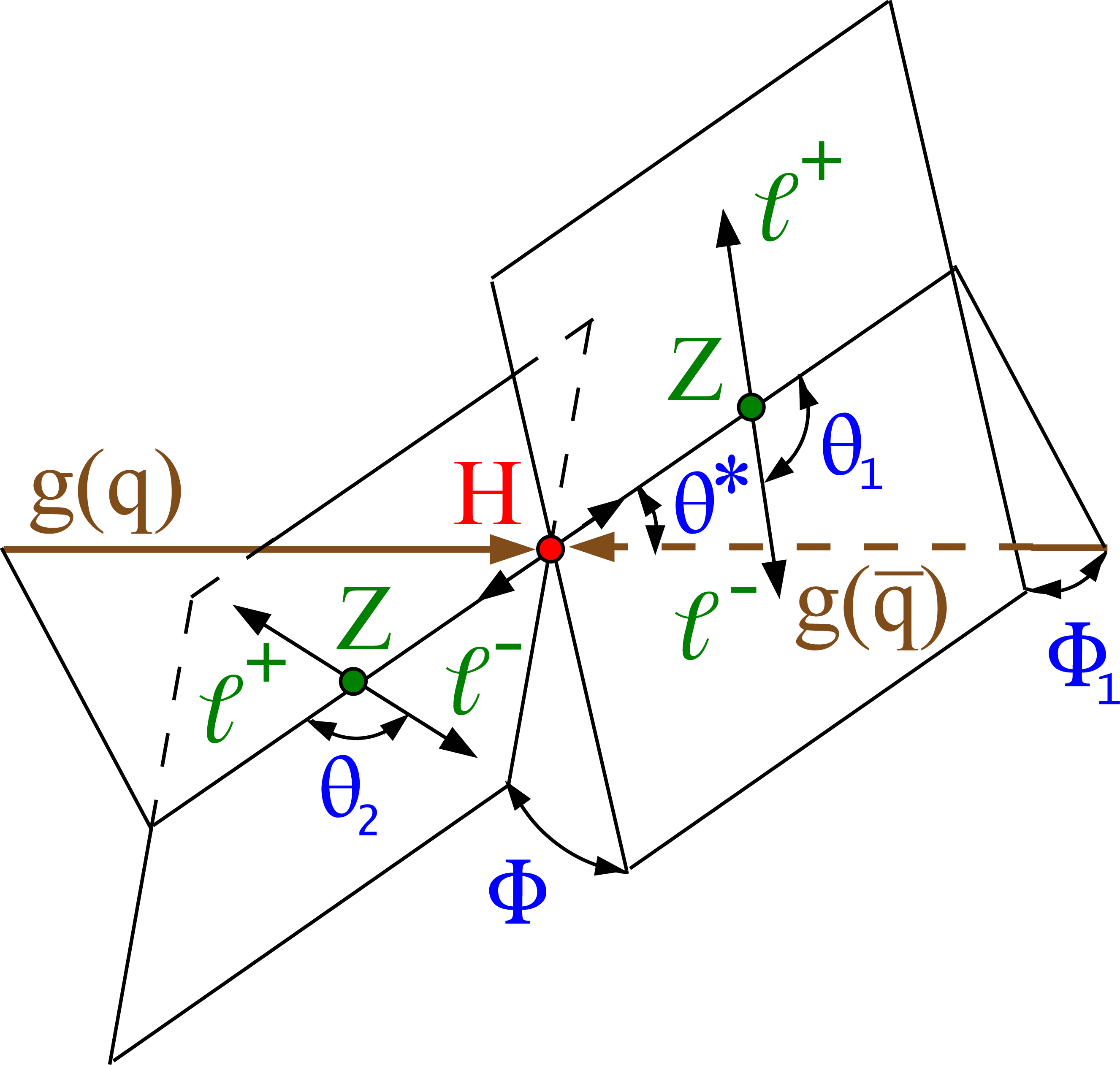
Figure 1-a:
Illustration of H particle production and decay $gg/\mathrm{q\bar{q}}\to \mathrm{ H } \to ZZ\to 4\ell ^\pm $. Angles and invariant masses fully characterize the orientation of the production and decay chain and are defined in the suitable rest frames [32,41,47]. |
png pdf |
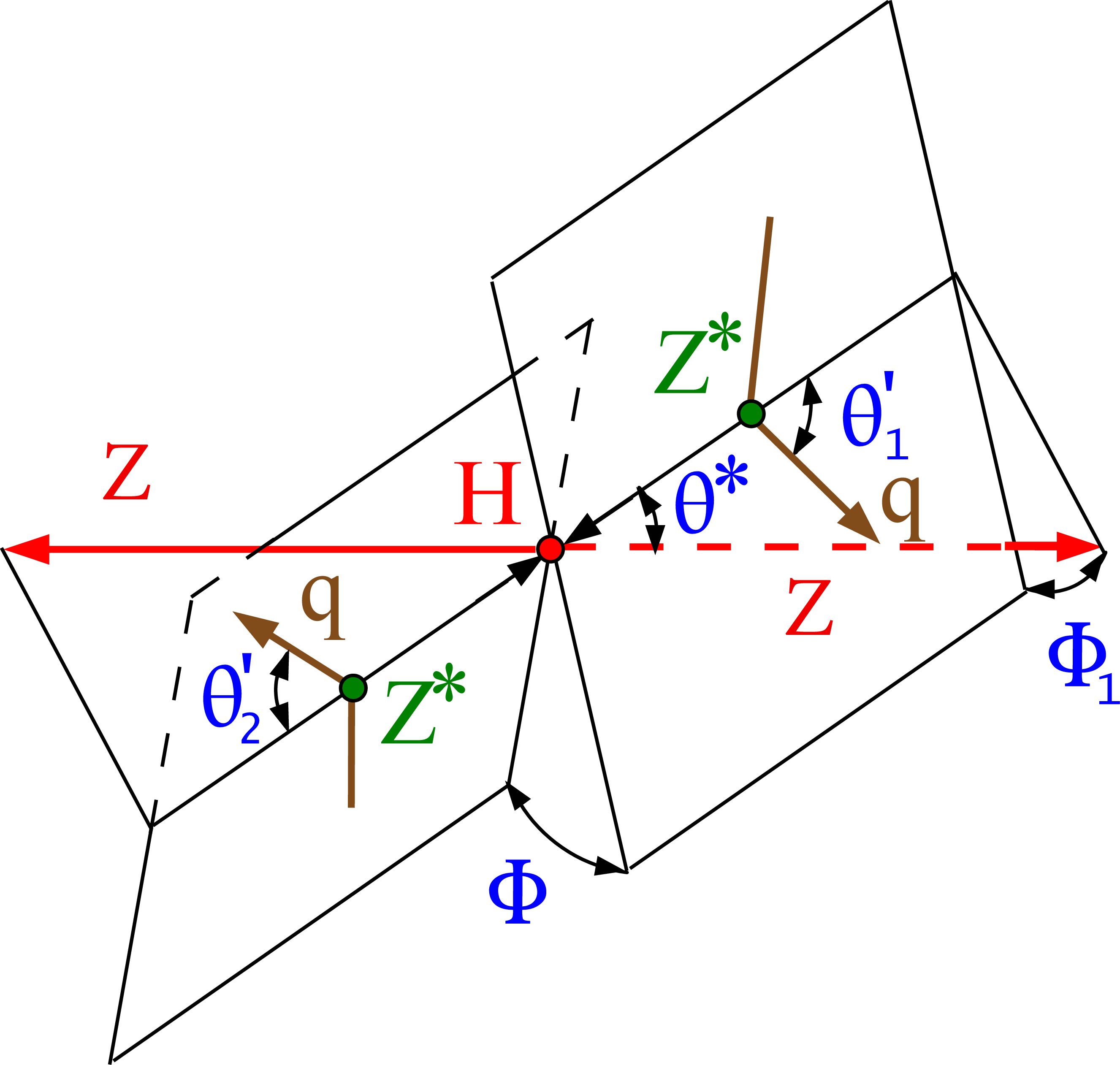
Figure 1-b:
Illustration of H particle production and decay VBF $q{q^\prime }\to q{q^\prime } \mathrm{ H } $. Angles and invariant masses fully characterize the orientation of the production and decay chain and are defined in the suitable rest frames [32,41,47]. |
png pdf |
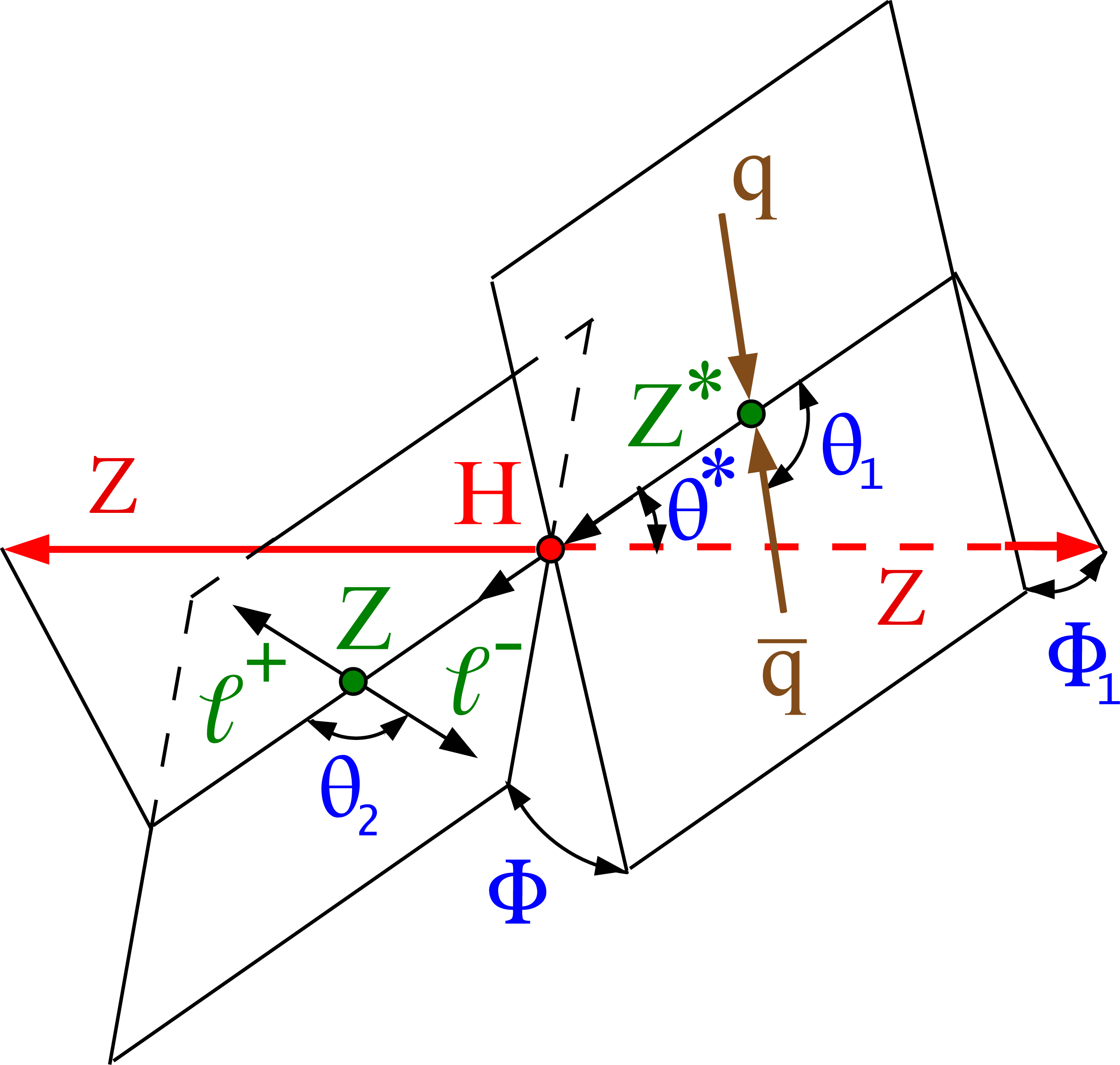
Figure 1-c:
Illustration of H particle production and decay $\mathrm{q\bar{q}}\to V^*\to VH$. Angles and invariant masses fully characterize the orientation of the production and decay chain and are defined in the suitable rest frames [32,41,47]. |

png pdf |
Figure 1-d:
Illustration of H particle production and decay $\mathrm{gg}/\mathrm{q\bar{q}}\to t\bar{t} \mathrm{ H } $. Angles and invariant masses fully characterize the orientation of the production and decay chain and are defined in the suitable rest frames [32,41,47]. |

png pdf |
Figure 2:
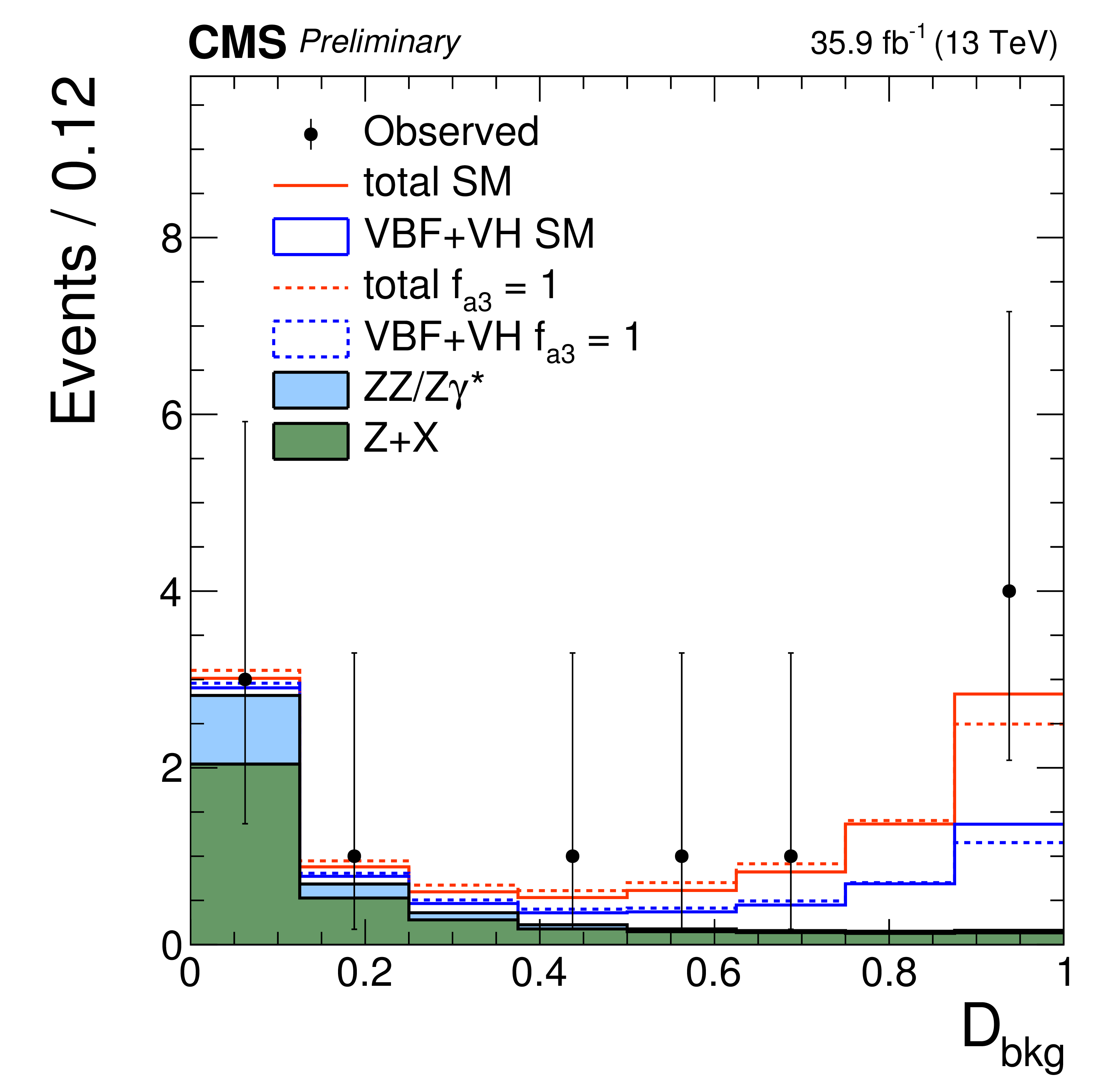
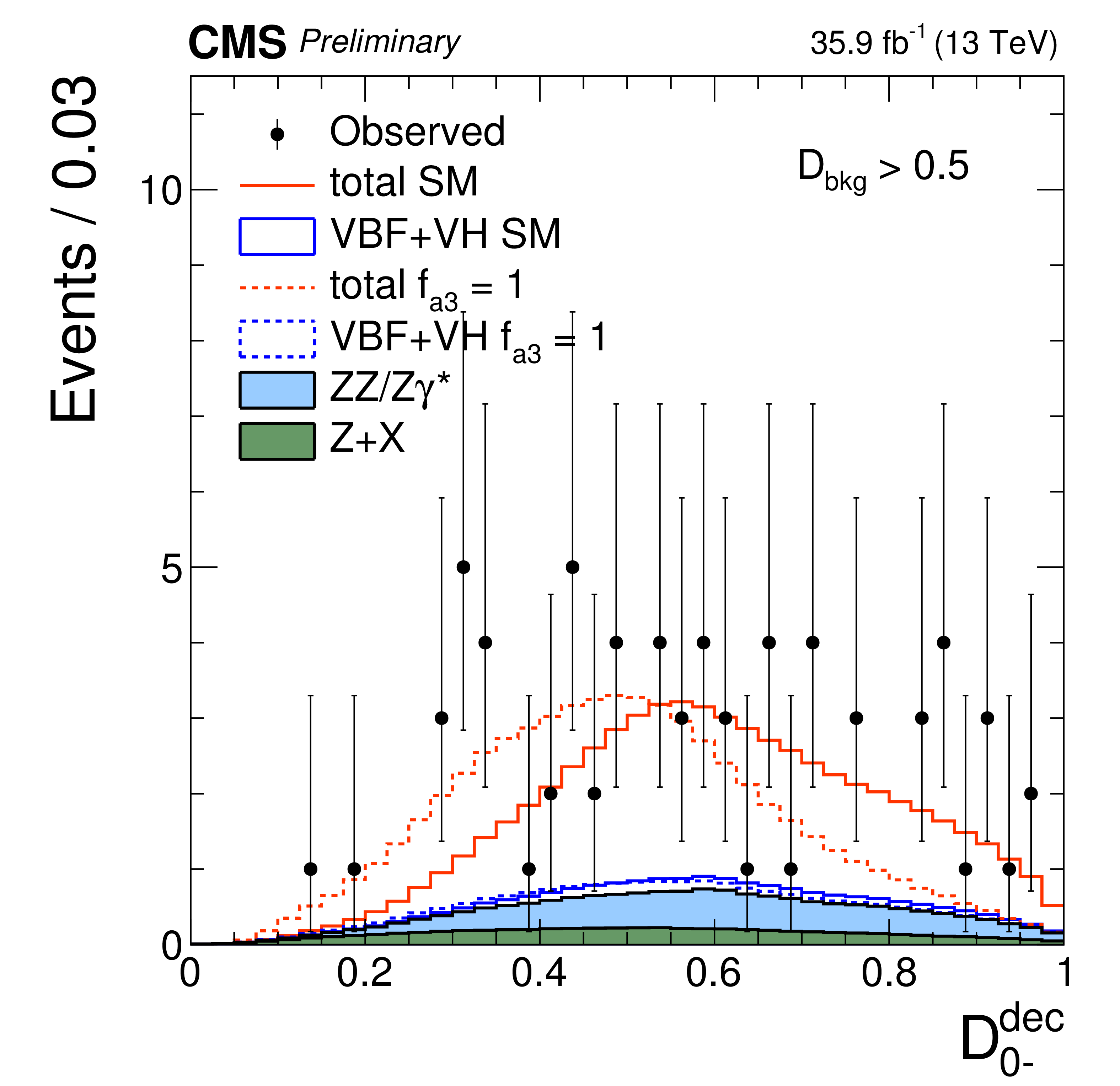
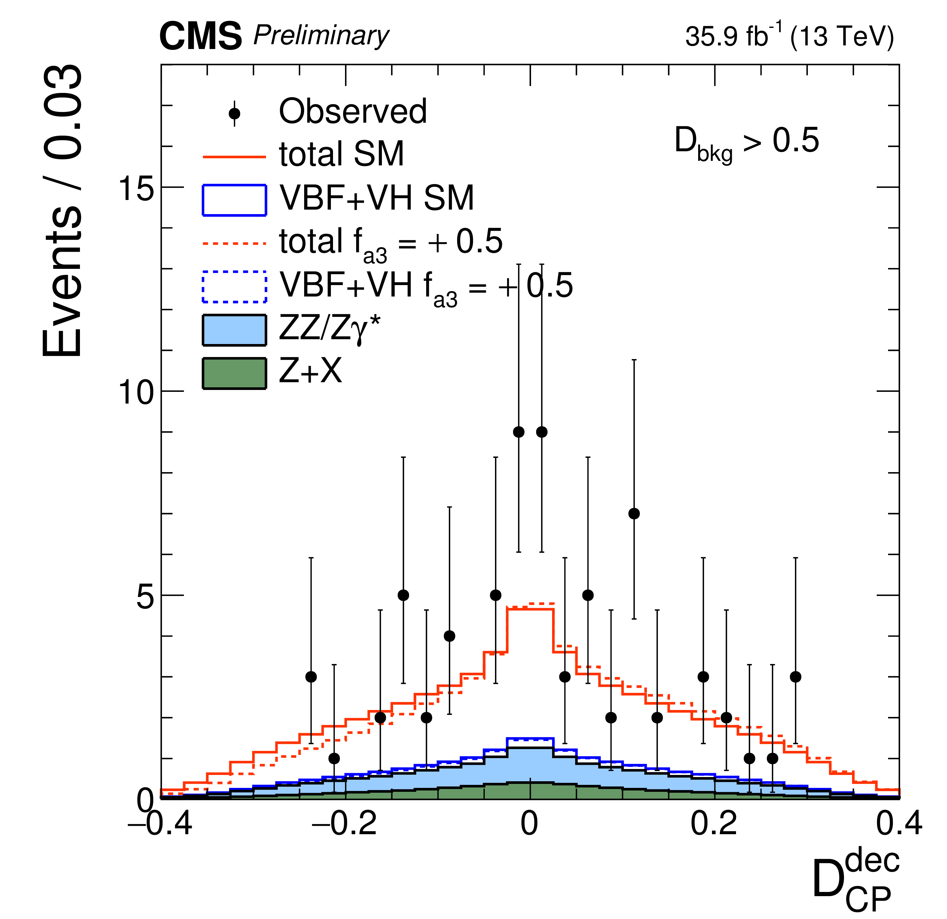
Distributions of kinematic discriminants in the $f_{a3}$ analysis: $\mathcal {D}_{\rm bkg}$ (left), $\mathcal {D}_{0-}$ (middle), and $\mathcal {D}_{CP}$ (right). The decay or production information used in the $\mathcal {D}_{0-}$ and $\mathcal {D}_{CP}$ discriminants is reflected in the superscript label and depends on the tagging category as summarized in Table 3. Three tagging categories are shown: VBF-jets (top), $ {\mathrm {V}} \mathrm{ H } $-jets (middle), and untagged (bottom). Points with error bars show data and histograms show expectations for background and SM or BSM signal as indicated in the legend. |
png pdf |
Figure 2-a:
Distribution of the $\mathcal {D}_{\rm bkg}$ kinematic discriminant in the $f_{a3}$ analysis for tagging category "VBF-jets". Points with error bars show data and histograms show expectations for background and SM or BSM signal as indicated in the legend. |
png pdf |
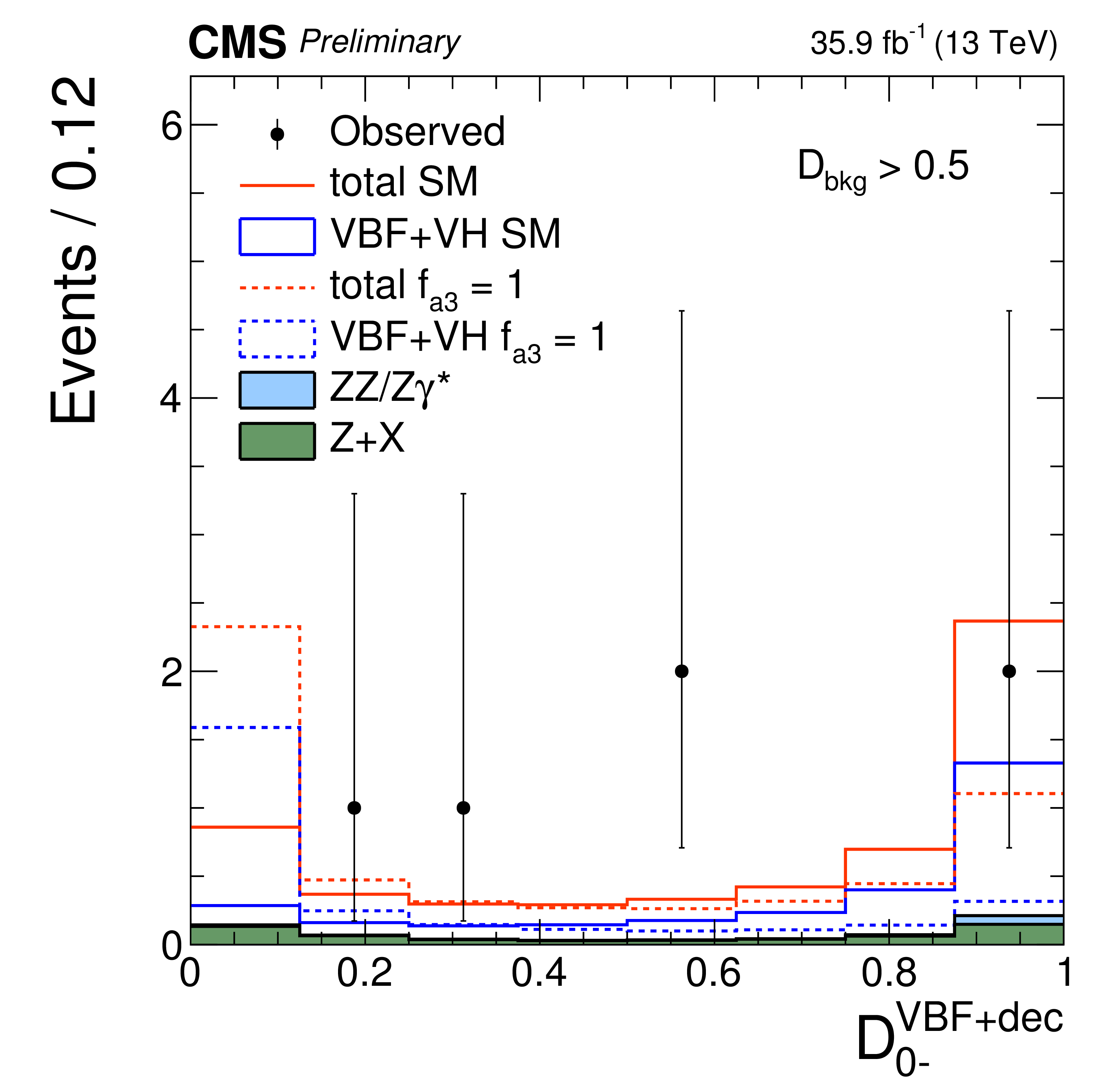
Figure 2-b:
Distribution of the $\mathcal {D}_{0-}$ kinematic discriminant in the $f_{a3}$ analysis for tagging category "VBF-jets". The decay or production information used in the discriminant is reflected in the superscript label and depends on the tagging category as summarized in Table 3. Points with error bars show data and histograms show expectations for background and SM or BSM signal as indicated in the legend. |

png pdf |
Figure 2-c:
Distribution of the $\mathcal {D}_{CP}$ kinematic discriminant in the $f_{a3}$ analysis for tagging category "VBF-jets". The decay or production information used in the discriminant is reflected in the superscript label and depends on the tagging category as summarized in Table 3. Points with error bars show data and histograms show expectations for background and SM or BSM signal as indicated in the legend. |
png pdf |
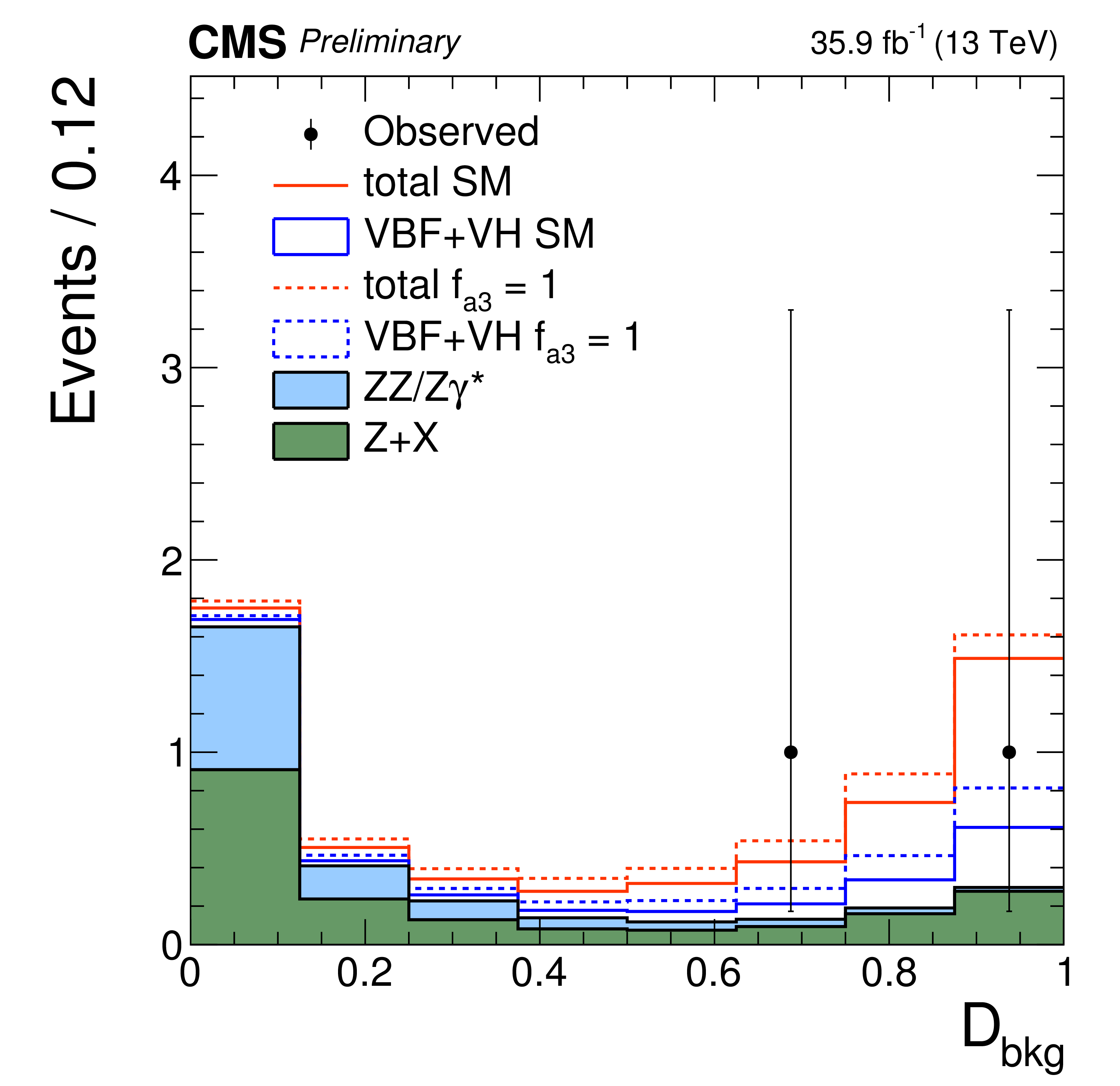
Figure 2-d:
Distribution of the $\mathcal {D}_{\rm bkg}$ kinematic discriminant in the $f_{a3}$ analysis for tagging category "$ {\mathrm {V}} \mathrm{ H } $-jets". Points with error bars show data and histograms show expectations for background and SM or BSM signal as indicated in the legend. |

png pdf |
Figure 2-e:
Distribution of the $\mathcal {D}_{0-}$ kinematic discriminant in the $f_{a3}$ analysis for tagging category "$ {\mathrm {V}} \mathrm{ H } $-jets". The decay or production information used in the discriminant is reflected in the superscript label and depends on the tagging category as summarized in Table 3. Points with error bars show data and histograms show expectations for background and SM or BSM signal as indicated in the legend. |
png pdf |
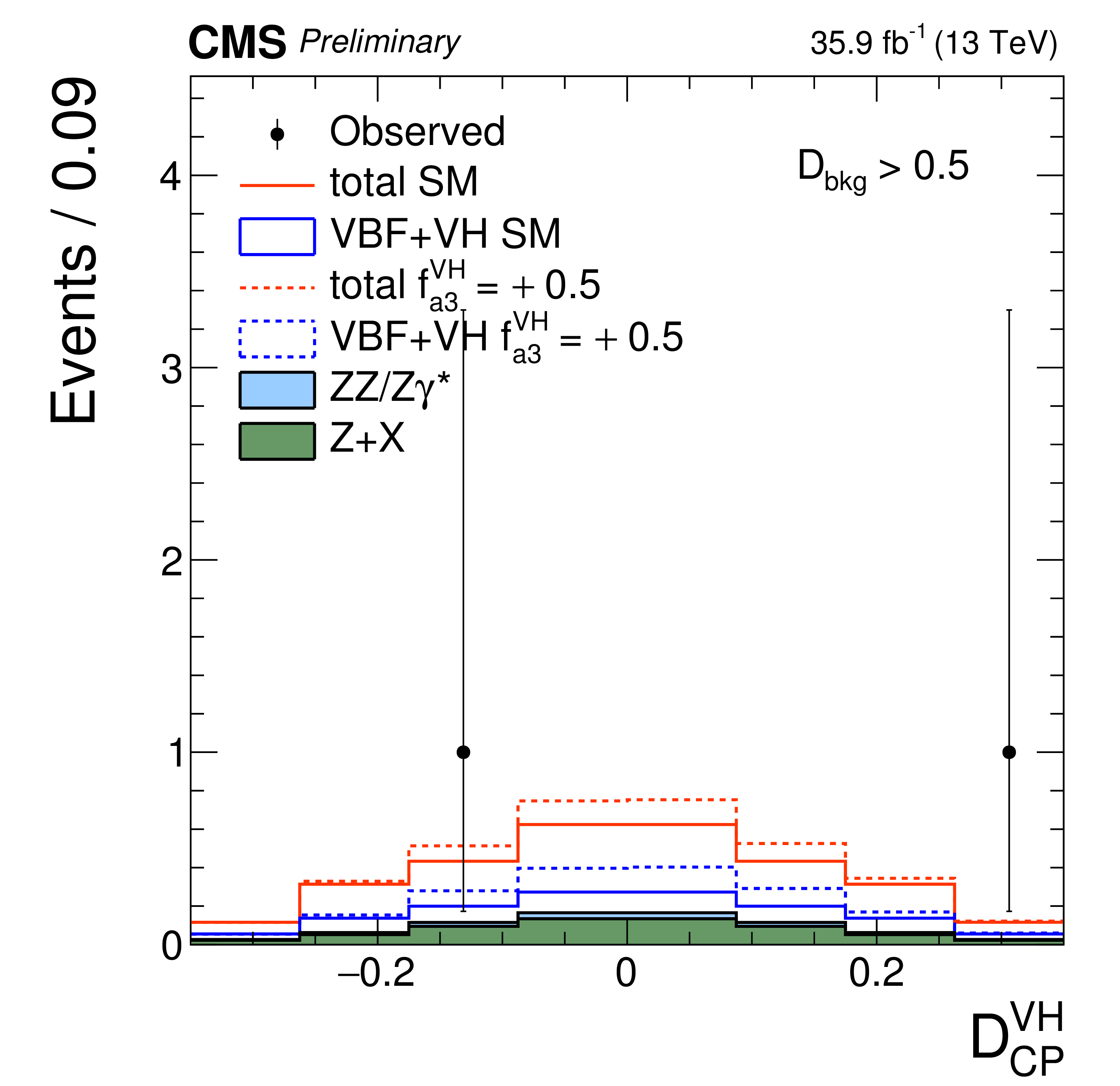
Figure 2-f:
Distribution of the $\mathcal {D}_{CP}$ kinematic discriminant in the $f_{a3}$ analysis for tagging category "$ {\mathrm {V}} \mathrm{ H } $-jets". The decay or production information used in the discriminant is reflected in the superscript label and depends on the tagging category as summarized in Table 3. Points with error bars show data and histograms show expectations for background and SM or BSM signal as indicated in the legend. |

png pdf |
Figure 2-g:
Distribution of the $\mathcal {D}_{\rm bkg}$ kinematic discriminant in the $f_{a3}$ analysis for tagging category "untagged". Points with error bars show data and histograms show expectations for background and SM or BSM signal as indicated in the legend. |
png pdf |
Figure 2-h:
Distribution of the $\mathcal {D}_{0-}$ kinematic discriminant in the $f_{a3}$ analysis for tagging category "untagged". The decay or production information used in the discriminant is reflected in the superscript label and depends on the tagging category as summarized in Table 3. Points with error bars show data and histograms show expectations for background and SM or BSM signal as indicated in the legend. |
png pdf |
Figure 2-i:
Distribution of the $\mathcal {D}_{CP}$ kinematic discriminant in the $f_{a3}$ analysis for tagging category "untagged". The decay or production information used in the discriminant is reflected in the superscript label and depends on the tagging category as summarized in Table 3. Points with error bars show data and histograms show expectations for background and SM or BSM signal as indicated in the legend. |
png pdf |
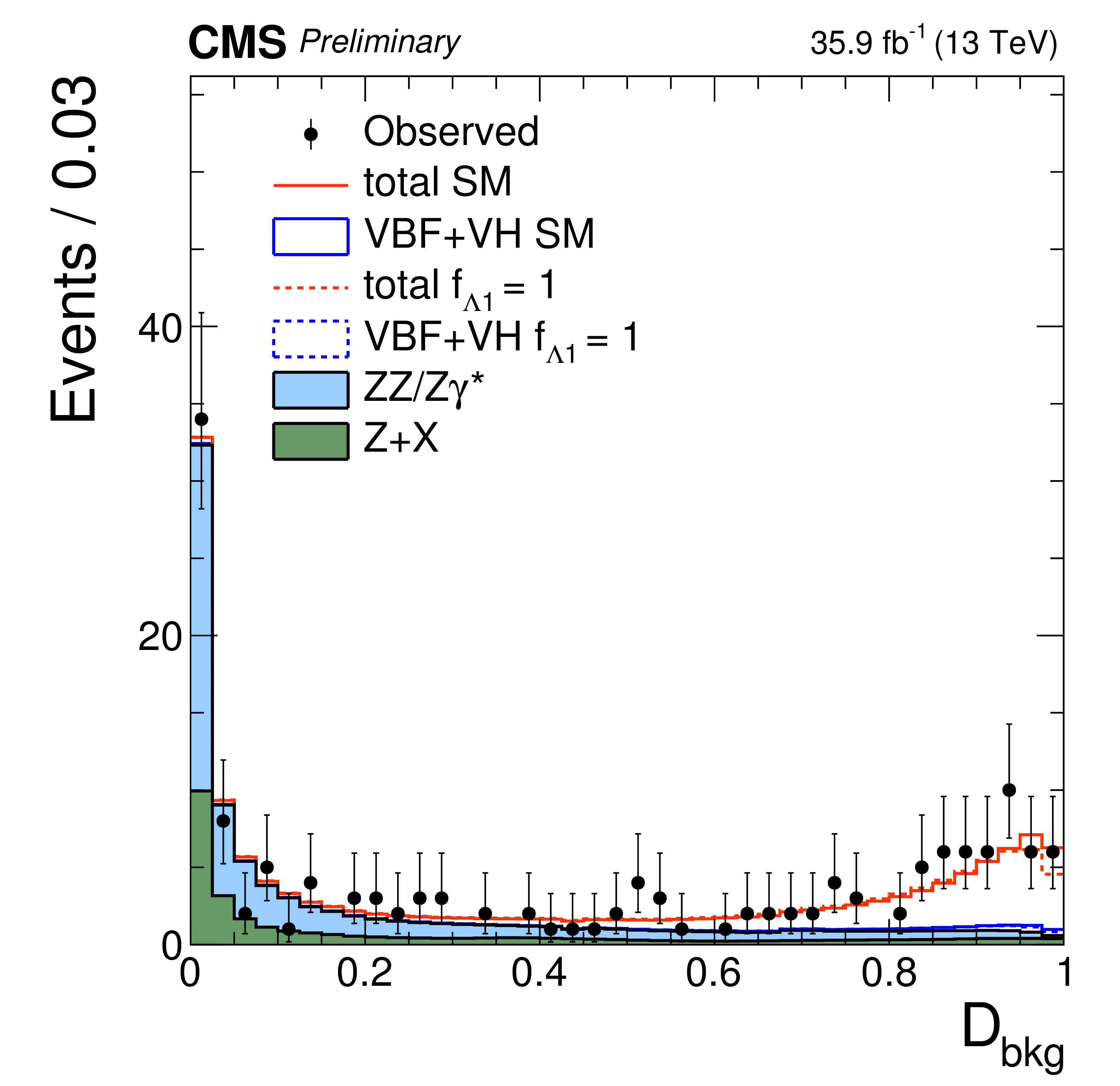
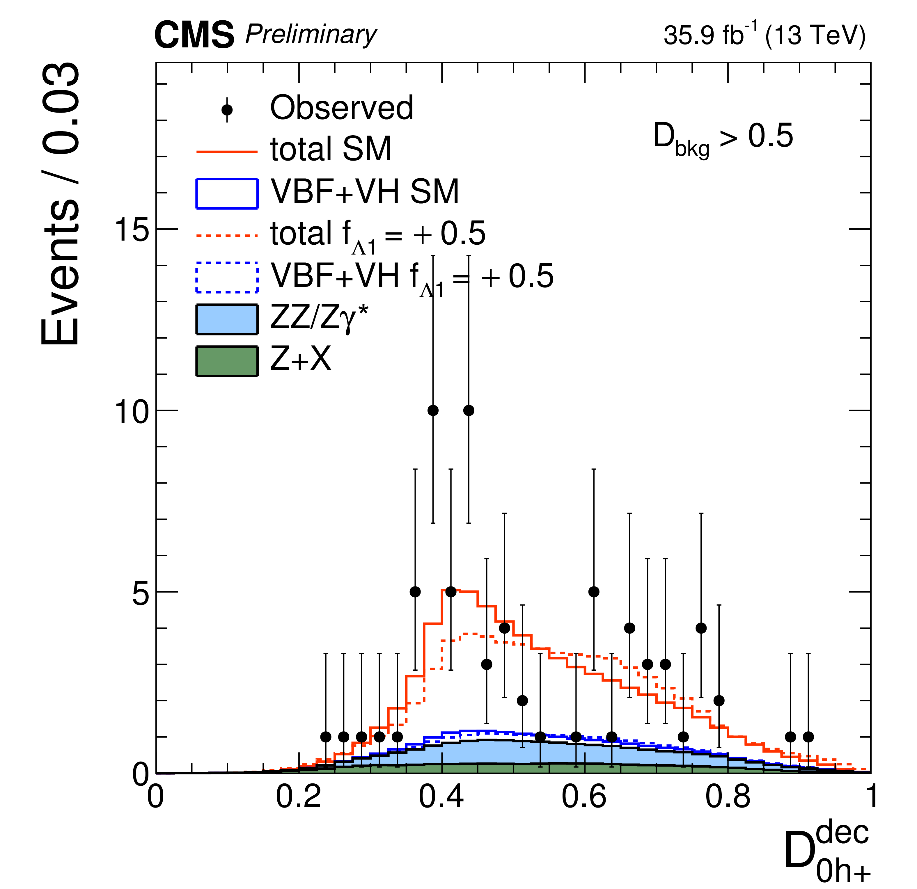
Figure 3:
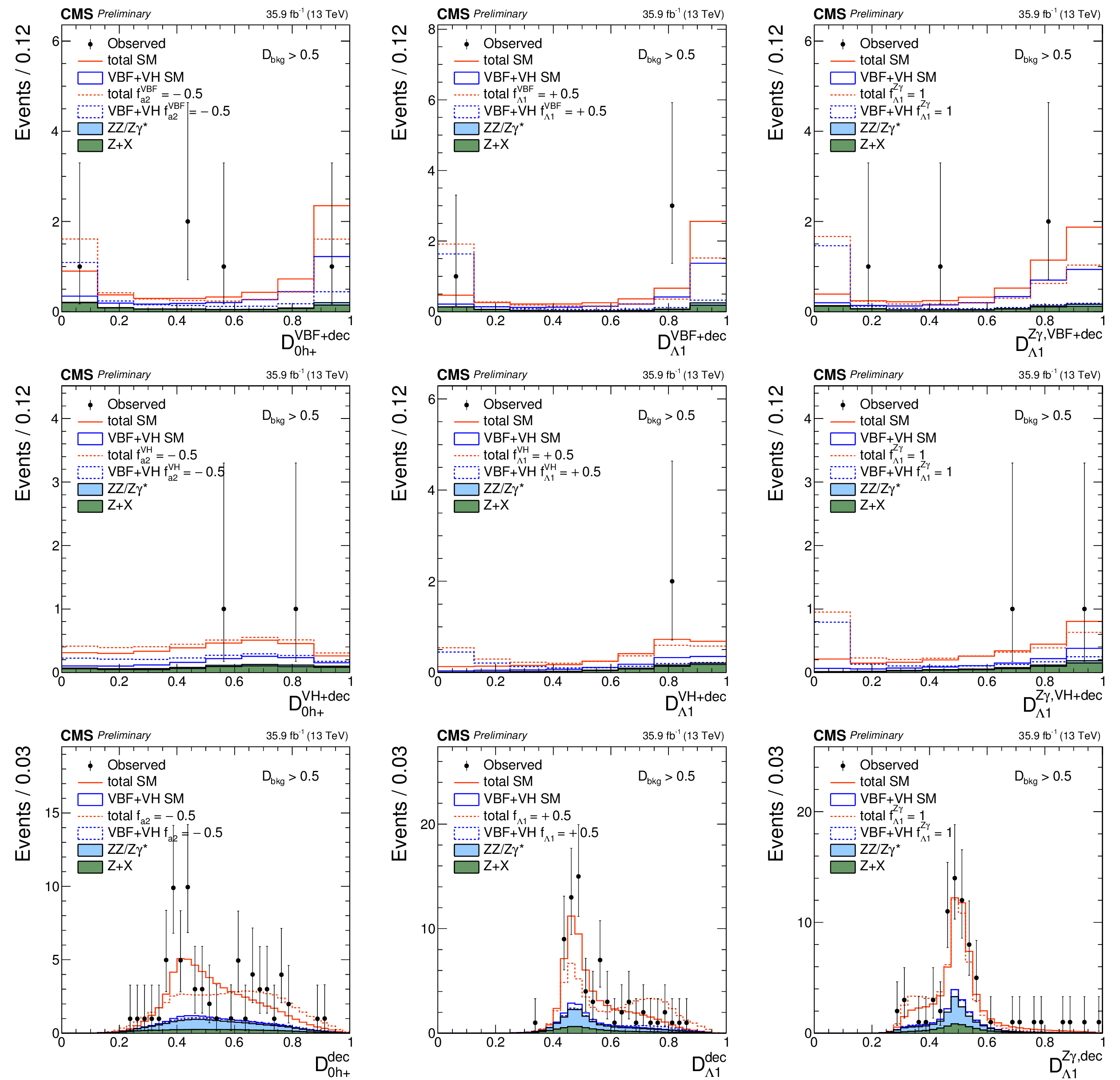
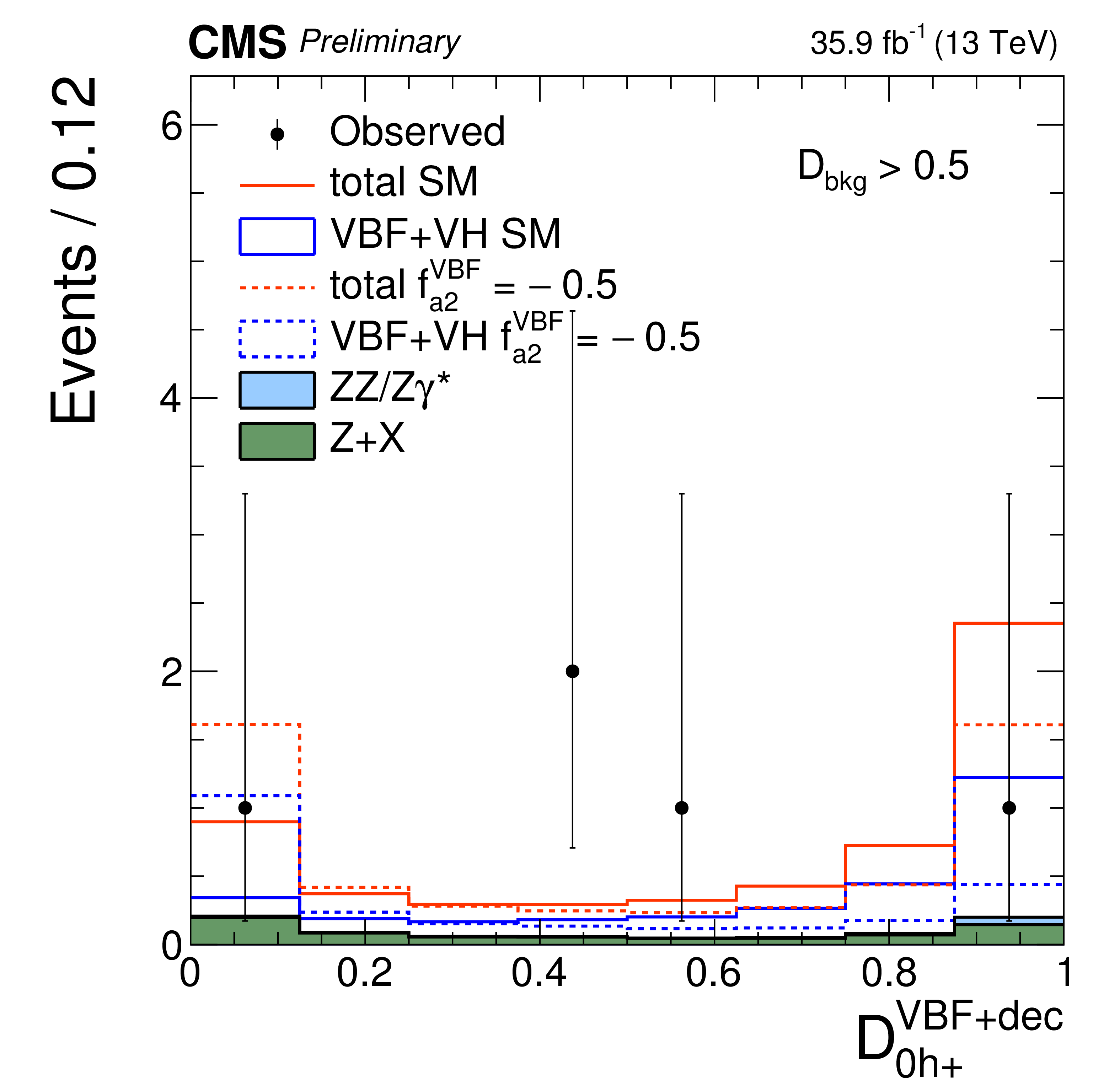
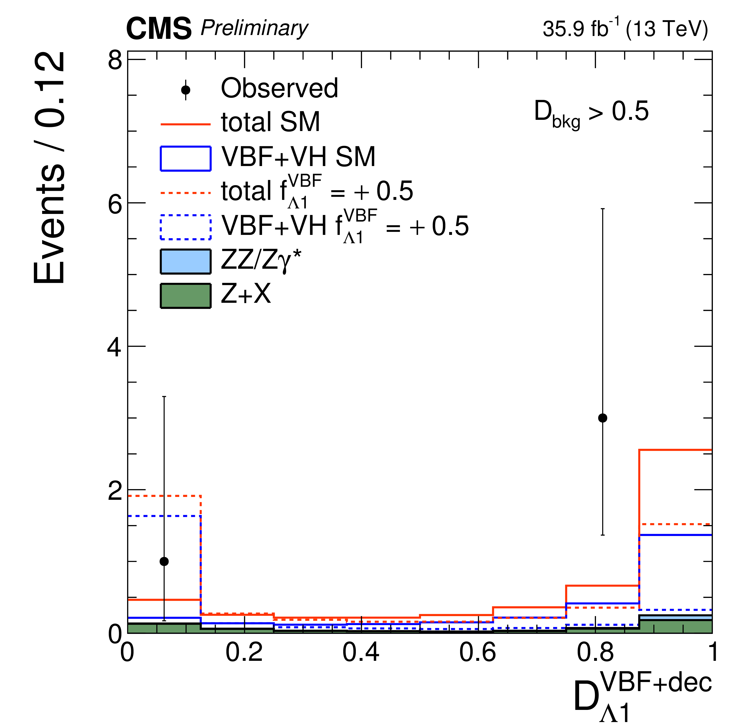
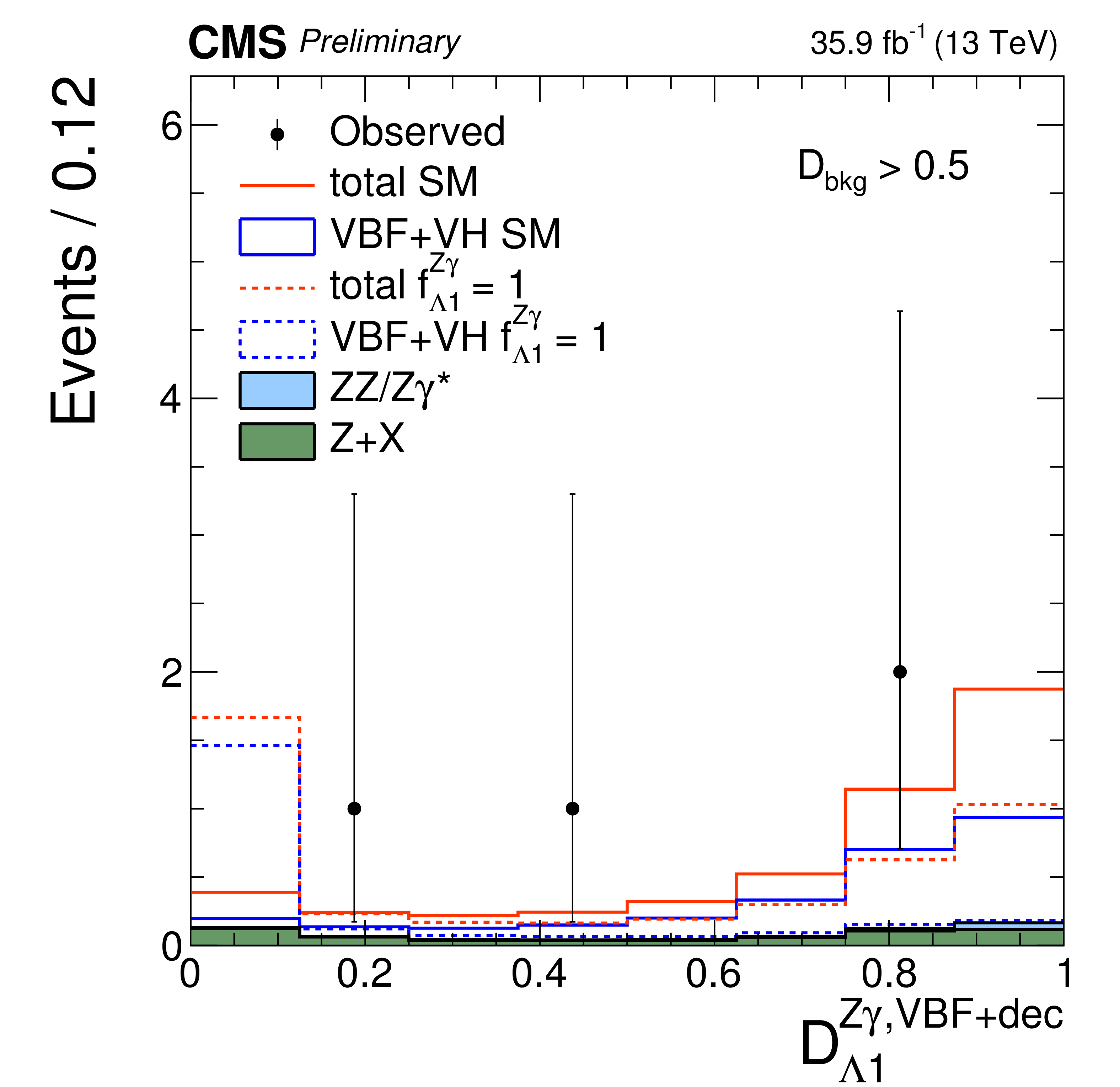
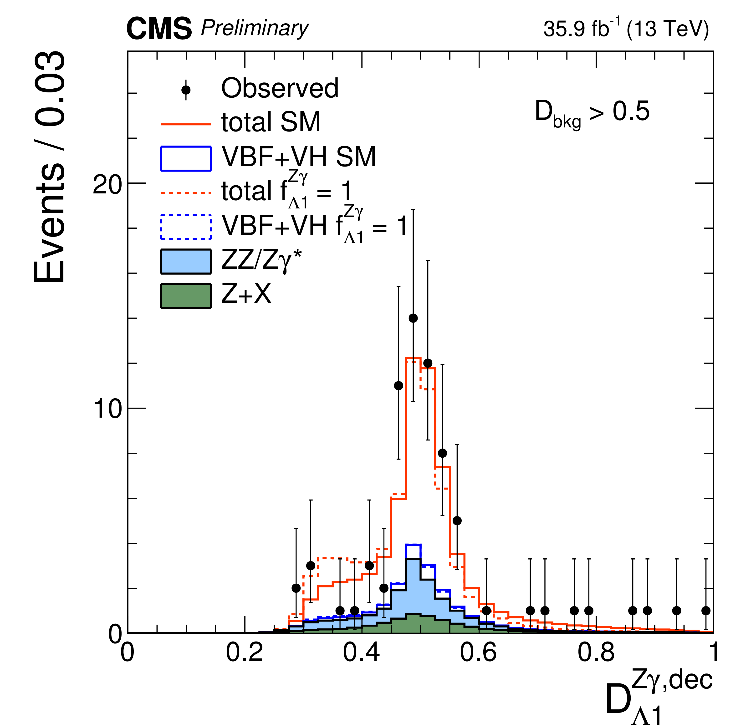
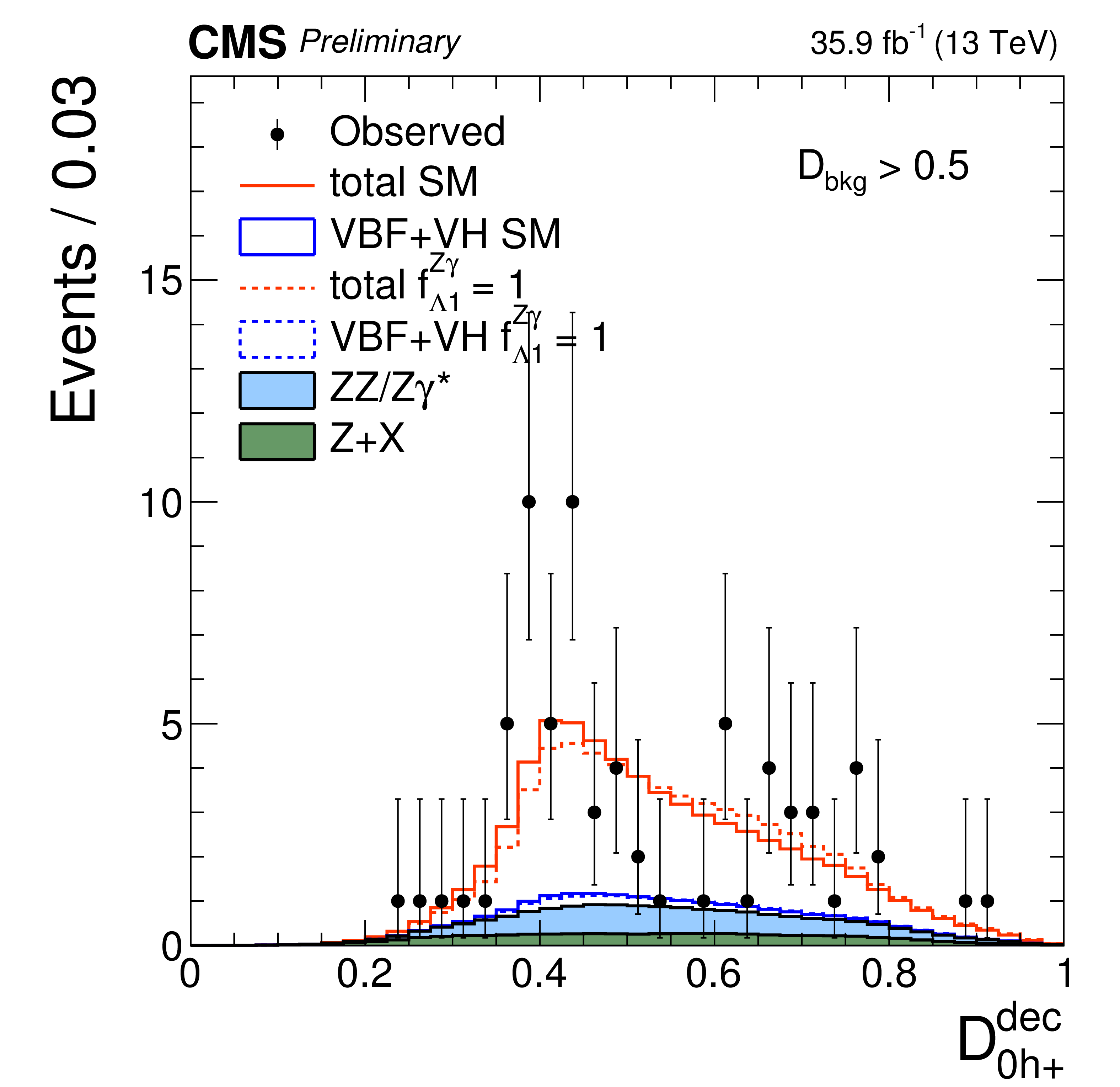
Distributions of kinematic discriminants in the $f_{a2}$ (left), $f_{\Lambda 1}$ (middle), and $f^{{\mathrm{ Z } } \gamma }_{\Lambda 1}$ (right) analyses: $\mathcal {D}_{0h+}$ (left), $\mathcal {D}_{\Lambda 1}$ (middle), and $\mathcal {D}^{{\mathrm{ Z } } \gamma }_{\Lambda 1}$ (right). The decay or production information used in the discriminants is reflected in the superscript label and depends on the tagging category as summarized in Table 3. Three tagging categories are shown: VBF-jets (top), $ {\mathrm {V}} \mathrm{ H } $-jets (middle), and untagged (bottom). Points with error bars show data and histograms show expectations for background and SM or BSM signal as indicated in the legend. |
png pdf |
Figure 3-a:
Distribution of the $\mathcal {D}_{0h+}$ kinematic discriminant in the $f_{a2}$ analysis, for tagging category "VBF-jets". The decay or production information used in the discriminant is reflected in the superscript label and depends on the tagging category as summarized in Table 3. Points with error bars show data and histograms show expectations for background and SM or BSM signal as indicated in the legend. |
png pdf |
Figure 3-b:
Distribution of the $\mathcal {D}_{\Lambda 1}$ kinematic discriminant in the $f_{\Lambda 1}$ analysis, for tagging category |
png pdf |
Figure 3-c:
Distribution of the $\mathcal {D}^{{\mathrm{ Z } } \gamma }_{\Lambda 1}$ kinematic discriminant in the $f^{{\mathrm{ Z } } \gamma }_{\Lambda 1}$ analysis, for tagging category |

png pdf |
Figure 3-d:
Distribution of the $\mathcal {D}_{0h+}$ kinematic discriminant in the $f_{a2}$ analysis, for tagging category "$ {\mathrm {V}} \mathrm{ H } $". The decay or production information used in the discriminant is reflected in the superscript label and depends on the tagging category as summarized in Table 3. Points with error bars show data and histograms show expectations for background and SM or BSM signal as indicated in the legend. |

png pdf |
Figure 3-e:
Distribution of the $\mathcal {D}_{\Lambda 1}$ kinematic discriminant in the $f_{\Lambda 1}$ analysis, for tagging category "$ {\mathrm {V}} \mathrm{ H } $". The decay or production information used in the discriminant is reflected in the superscript label and depends on the tagging category as summarized in Table 3. Points with error bars show data and histograms show expectations for background and SM or BSM signal as indicated in the legend. |

png pdf |
Figure 3-f:
Distribution of the $\mathcal {D}^{{\mathrm{ Z } } \gamma }_{\Lambda 1}$ kinematic discriminant in the $f^{{\mathrm{ Z } } \gamma }_{\Lambda 1}$ analysis, for tagging category "$ {\mathrm {V}} \mathrm{ H } $" |

png pdf |
Figure 3-g:
Distribution of the $\mathcal {D}_{0h+}$ kinematic discriminant in the $f_{a2}$ analysis, for tagging category "untagged". The decay or production information used in the discriminant is reflected in the superscript label and depends on the tagging category as summarized in Table 3. Points with error bars show data and histograms show expectations for background and SM or BSM signal as indicated in the legend. |

png pdf |
Figure 3-h:
Distribution of the $\mathcal {D}_{\Lambda 1}$ kinematic discriminant in the $f_{\Lambda 1}$ analysis, for tagging category "untagged". The decay or production information used in the discriminant is reflected in the superscript label and depends on the tagging category as summarized in Table 3. Points with error bars show data and histograms show expectations for background and SM or BSM signal as indicated in the legend. |
png pdf |
Figure 3-i:
Distribution of the $\mathcal {D}^{{\mathrm{ Z } } \gamma }_{\Lambda 1}$ kinematic discriminant in the |
png pdf |
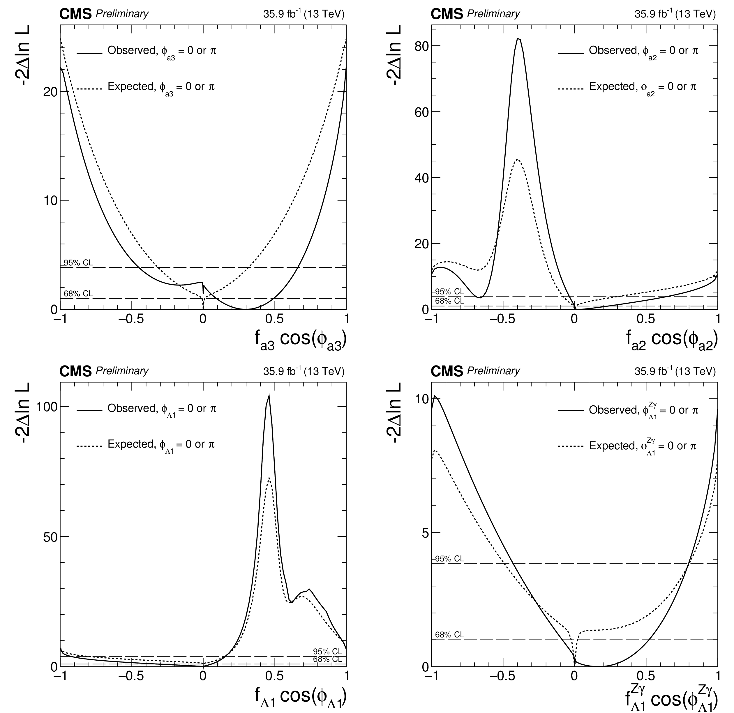
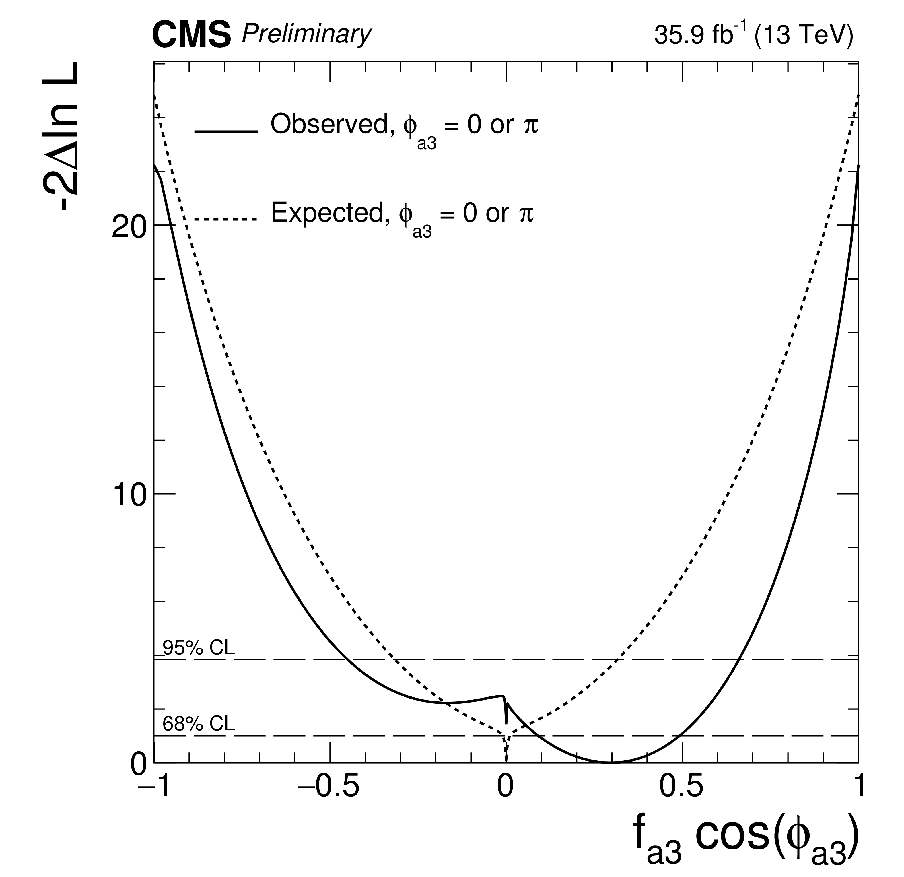
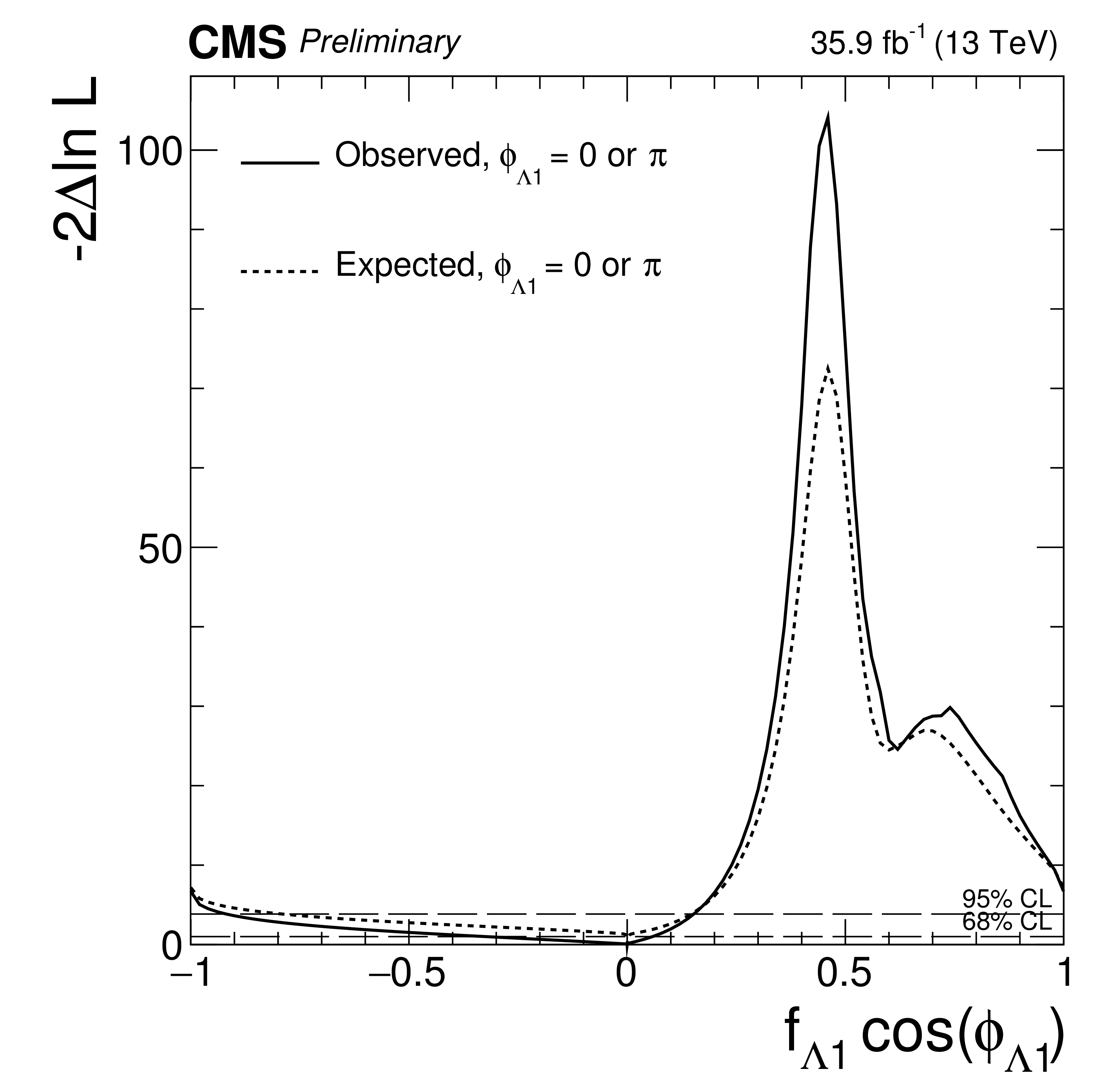
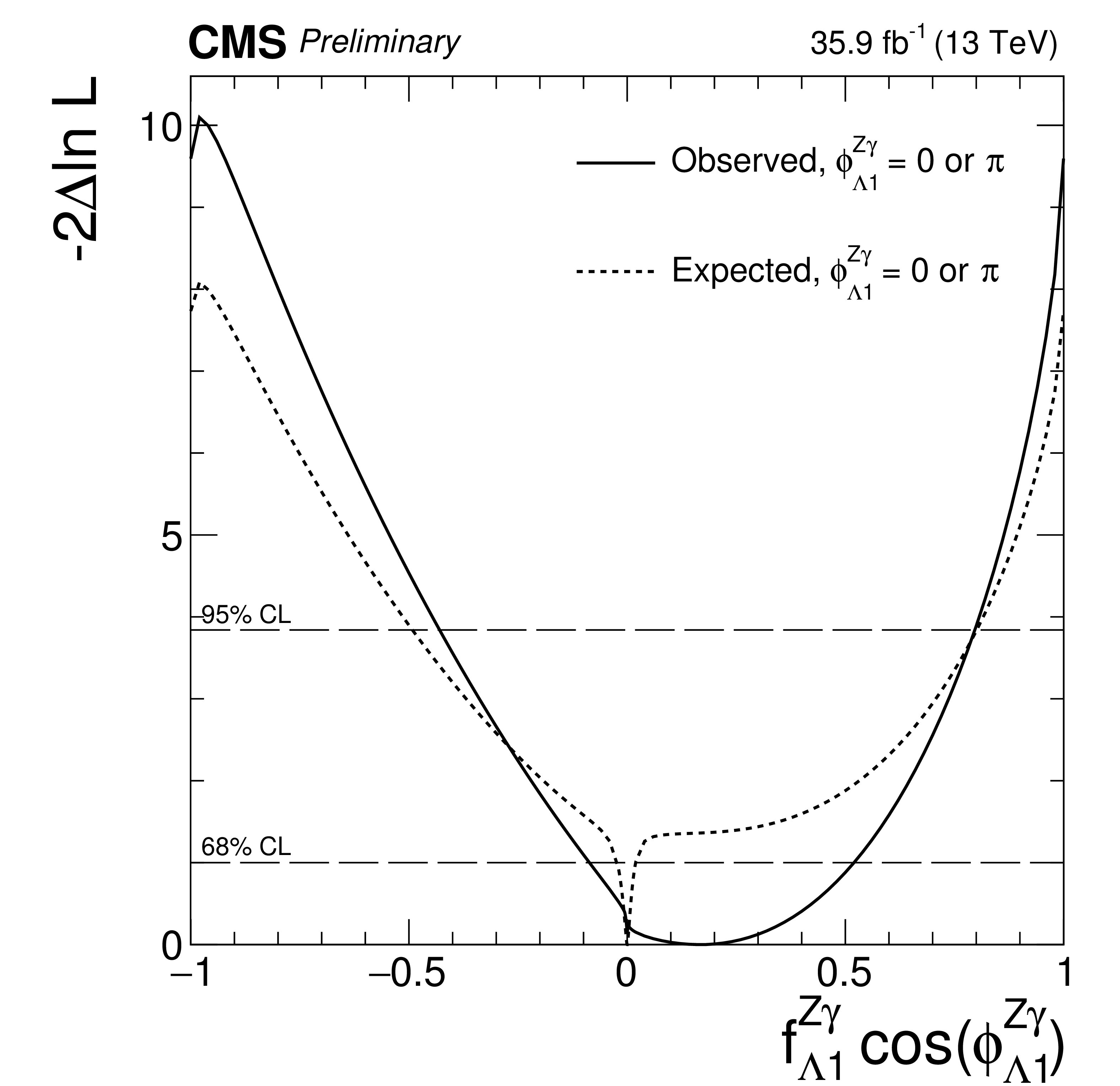
Figure 4:
Observed (solid) and expected (dashed) likelihood scan of the $f_{a3}\cos(\phi _{a3})$ (top-left), $f_{a2}\cos(\phi _{a2})$ (top-right), $f_{\Lambda 1}\cos(\phi _{\Lambda 1})$ (bottom-left), and $f_{\Lambda 1}^{{\mathrm{ Z } } \gamma }\cos(\phi _{\Lambda 1}^{{\mathrm{ Z } } \gamma })$ (bottom-right) parameters with 35.9 fb$^{-1}$ of data at 13 TeV. It is assumed that ratios of anomalous couplings are real and therefore $\cos(\phi _{an})= \pm$1. |
png pdf |
Figure 4-a:
Observed (solid) and expected (dashed) likelihood scan of the $f_{a3}\cos(\phi _{a3})$ parameter with 35.9 fb$^{-1}$ of data at 13 TeV. It is assumed that ratios of anomalous couplings are real and therefore $\cos(\phi _{an})= \pm$1. |

png pdf |
Figure 4-b:
Observed (solid) and expected (dashed) likelihood scan of the $f_{a2}\cos(\phi _{a2})$ parameter with 35.9 fb$^{-1}$ of data at 13 TeV. It is assumed that ratios of anomalous couplings are real and therefore $\cos(\phi _{an})= \pm$1. |
png pdf |
Figure 4-c:
Observed (solid) and expected (dashed) likelihood scan of the $f_{\Lambda 1}\cos(\phi _{\Lambda 1})$ parameter with 35.9 fb$^{-1}$ of data at 13 TeV. It is assumed that ratios of anomalous couplings are real and therefore $\cos(\phi _{an})= \pm$1. |
png pdf |
Figure 4-d:
Observed (solid) and expected (dashed) likelihood scan of the $f_{\Lambda 1}^{{\mathrm{ Z } } \gamma }\cos(\phi _{\Lambda 1}^{{\mathrm{ Z } } \gamma })$ parameter with 35.9 fb$^{-1}$ of data at 13 TeV. It is assumed that ratios of anomalous couplings are real and therefore $\cos(\phi _{an})= \pm$1. |
| Tables | |

png pdf |
Table 1:
List of anomalous HVV couplings considered in the measurements assuming a spin-zero H boson. The definition of the effective fractions is discussed in the text and the translation constant is given in each case. The effective cross sections correspond to the processes $\mathrm{ H } \to 2\mathrm{ e } 2\mu $ and the Higgs boson mass assumed in this analysis $m_{\mathrm{ H } }=$ 125 GeV using the JHUGen [32,36,41] calculation. The cross-section ratios for the $\mathrm{ H } {\mathrm{ Z } } \gamma $ coupling include the requirement $\sqrt {|q^2_i|} \ge $ 4 GeV. |
png pdf |
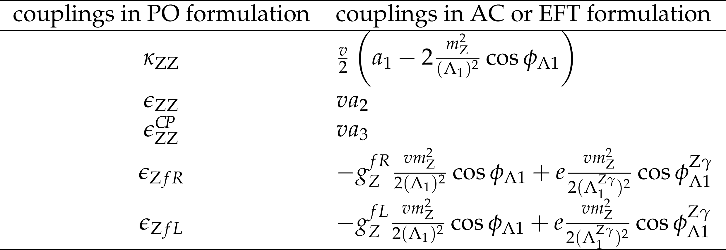
Table 2:
Translation between the couplings used in PO formulation [45,46] and couplings in AC or EFT formulation [20,21,22,23,24,25,26,27,28,29,30,31,32,33,34,35,36,37,38,39,40,41,42,43,44]. |
png pdf |
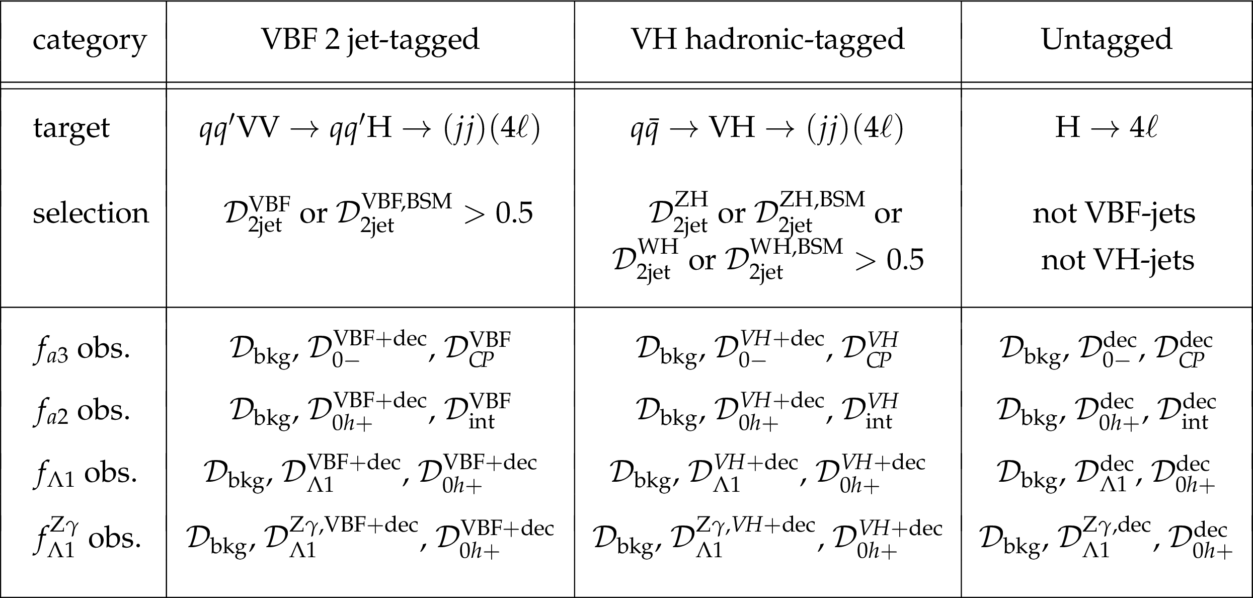
Table 3:
Summary of three production categories in analysis of the $\mathrm{ H } \to 4\ell $ events. The discriminants $\mathcal {D}$ based on the matrix element likelihood calculations are defined for each category of events as discussed in text. Three BSM models are considered in definition of the categories: $f_{a3}=$ 1, $f_{a2}=$ 1, $f_{\Lambda 1}=$ 1, and $f^{{\mathrm{ Z } } \gamma }_{\Lambda 1}=$ 1. Three observables (abbreviated as obs.) are listed for each analysis and for each category. The $\mathcal {D}_{0h+}$ discriminant is used in the $f_{\Lambda 1}$ and $f^{{\mathrm{ Z } } \gamma }_{\Lambda 1}$ measurements to allow a two-parameter fit together with $f_{a2}$ at a later time. |
png pdf |
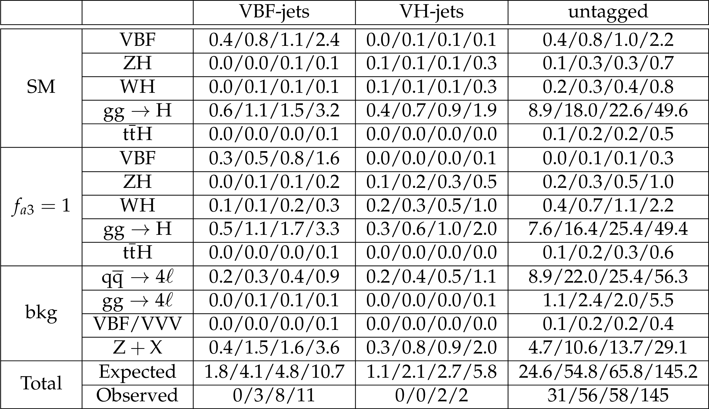
Table 4:
Expected and observed number of events across the three categories for different signal and background production modes, using categorization as defined for the $f_{a3}$ analysis. The yields for the $f_{a3}=1$ hypothesis are normalized so that the total number of expected events for $\gamma \gamma \to \mathrm{ H } +{\mathrm{ t } {}\mathrm{ \bar{t} } } \mathrm{ H } $ and for $\text {VBF}+{\mathrm{ Z } } \mathrm{ H } +\mathrm{ W } \mathrm{ H } $ are as in the Standard Model. The numbers are quoted for the $4\mathrm{ e } $/$4\mu $/$2\mathrm{ e } 2\mu $/all final states. |
png pdf |
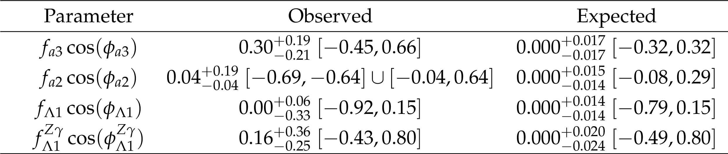
Table 5:
Summary of allowed 68%CL (central values with uncertainties) and 95%CL (ranges in square brackets) intervals on anomalous coupling parameters in HVV interactions under the assumption that all the coupling ratios are real ($\phi _{ai}^{ {\mathrm {V}} {\mathrm {V}} }=$ 0 or $\pi $). The expected results are quoted for the SM signal production cross section ($f_{an}=$ 0 and $\mu _V=\mu _f=$ 1). |
| Summary |
| In this note, the study of the anomalous interactions of the recently discovered Higgs boson is performed using the decay information $\mathrm{ H }\to 4\ell$ and information from associated production of two quark jets, originating either from vector boson fusion or associated vector boson. The full dataset recorded by the CMS experiment during 2016 of the LHC Run 2 is used, corresponding to an integrated luminosity of 35.9 fb$^{-1}$ at 13 TeV. Novel techniques are used for the study of associated VBF and VH production and its combination with analysis of decay information using optimal approaches based on matrix element techniques. The tensor structure of the interactions of the spin-zero Higgs boson with two vector bosons either in production or in decay is investigated and constraints are set on anomalous HVV interactions. All observations are consistent with the expectations for the standard model Higgs boson. |
| Additional Figures | |

png pdf |
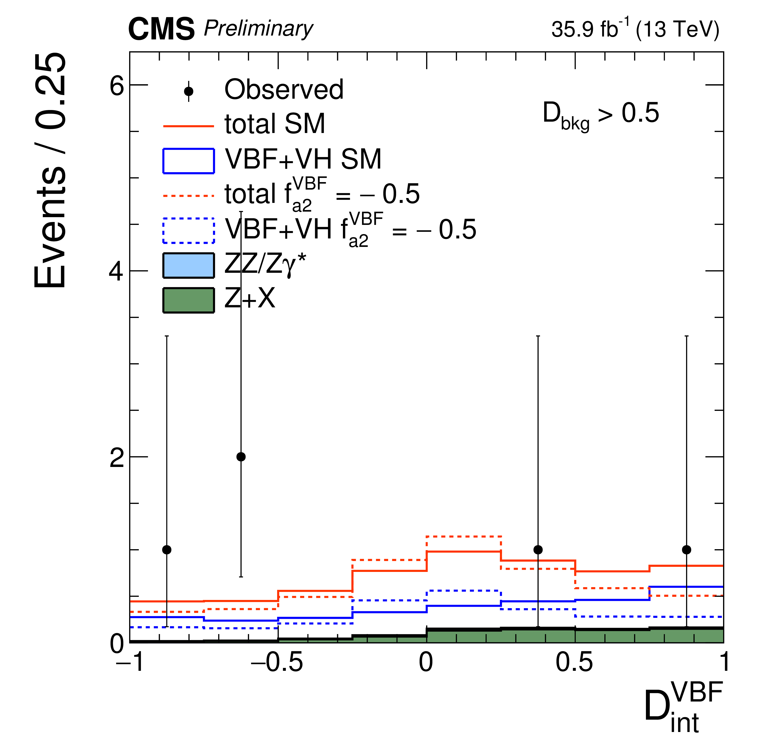
Additional Figure 1:
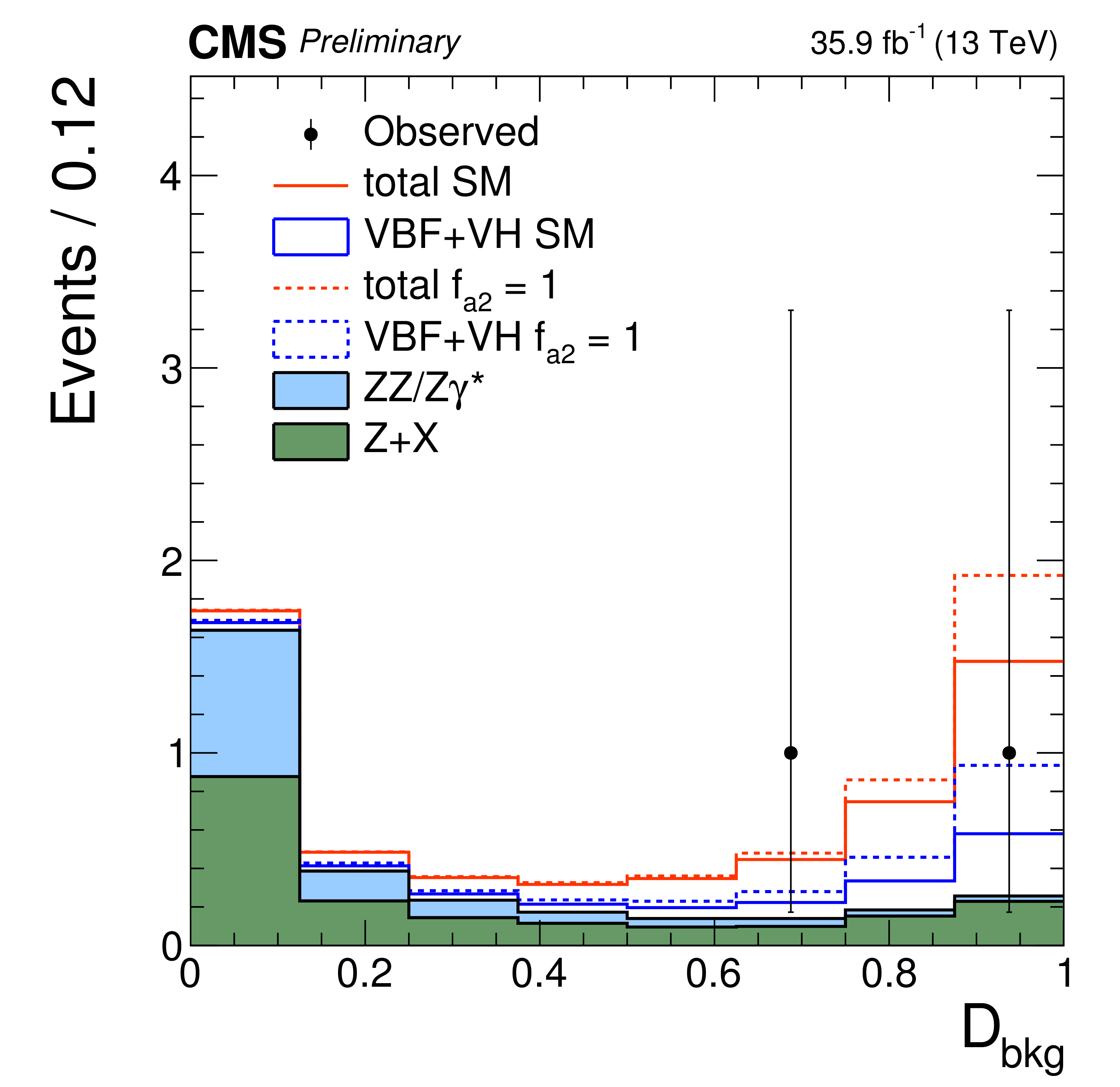
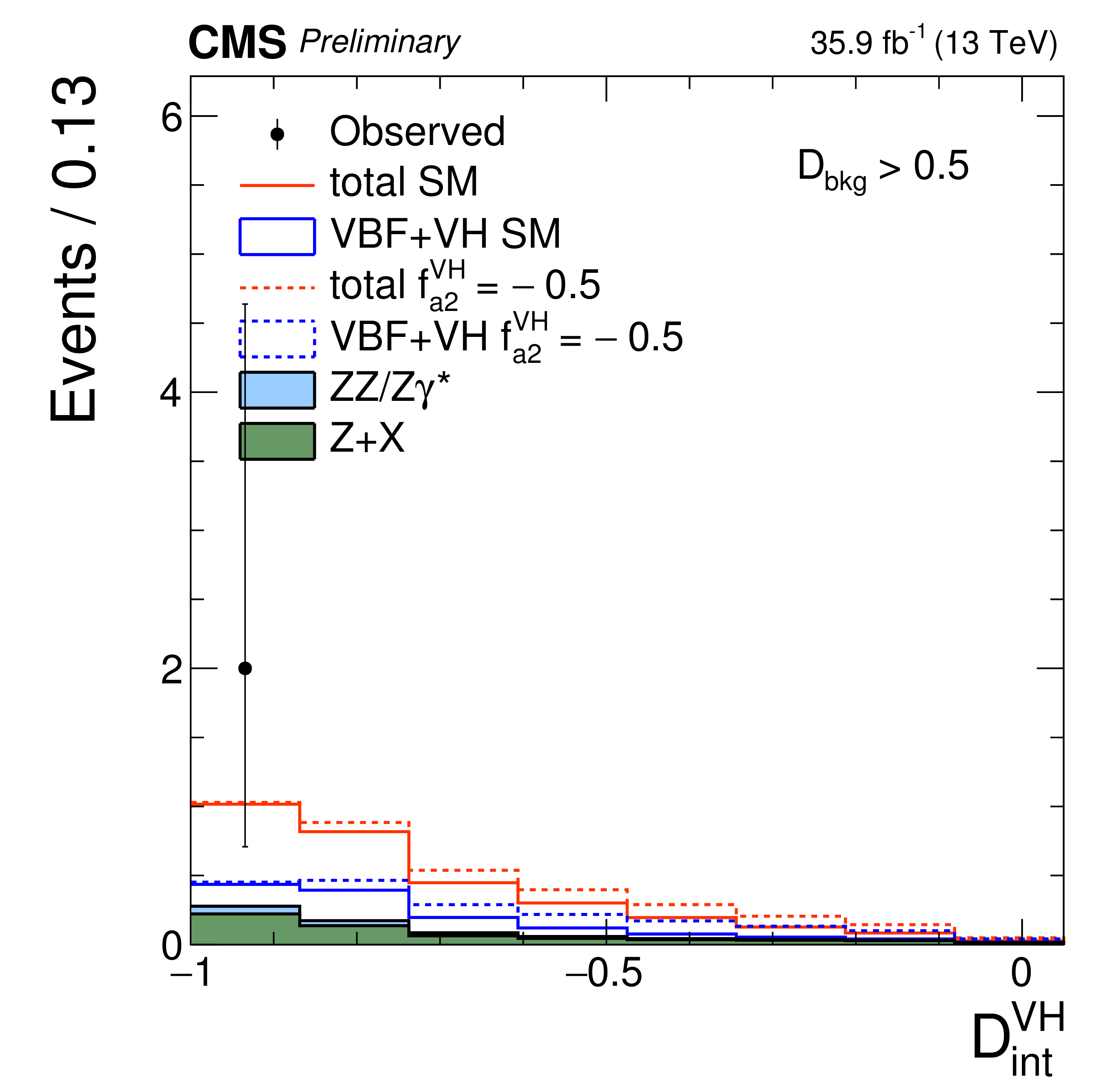
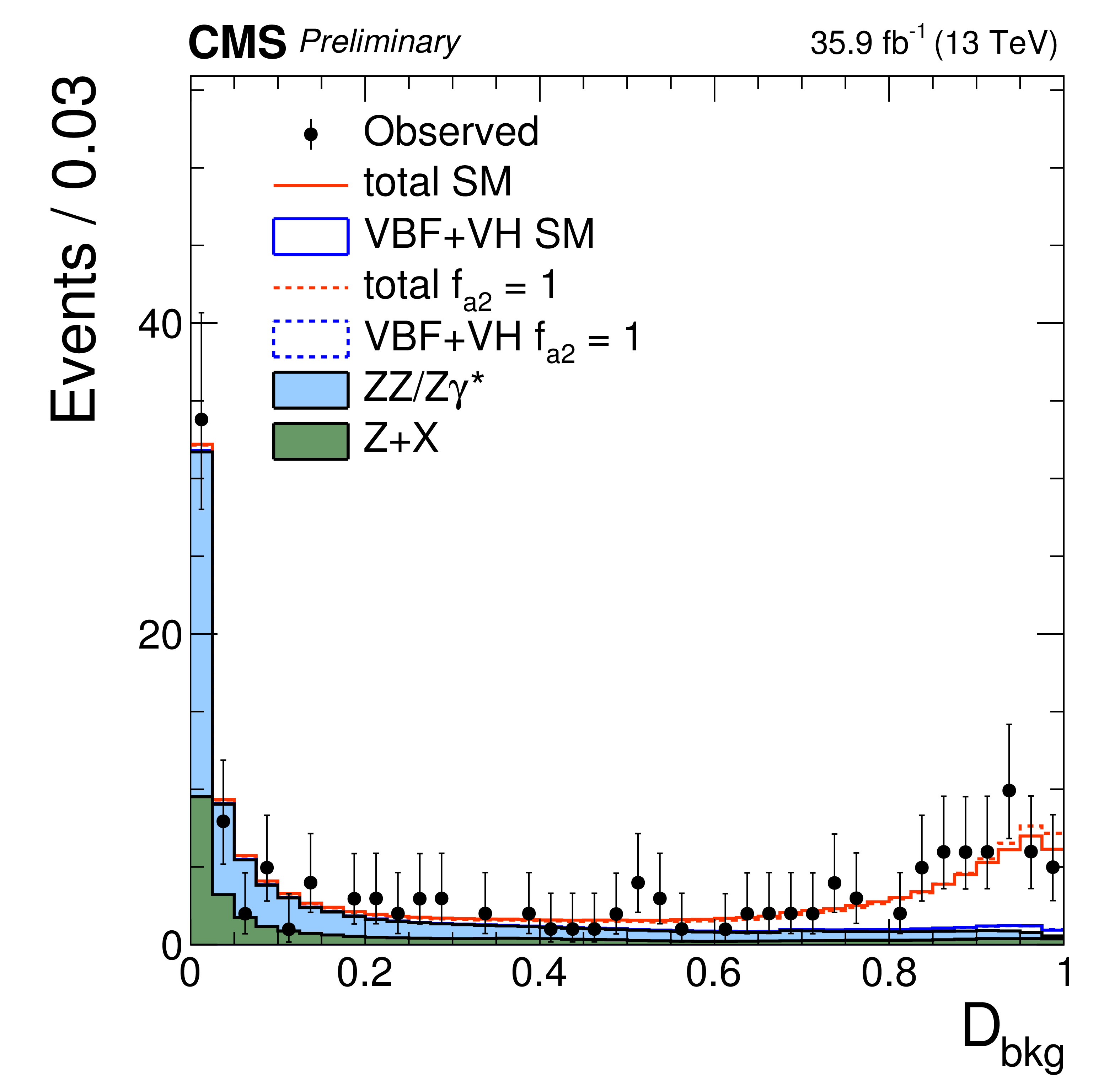
Distributions of kinematic discriminants in the $f_{a2}$ analysis: $\mathcal {D}_{\rm bkg}$ (a), (c), (e), and $\mathcal {D}_\text {int}$ (b), (d), (f). The decay or production information used in the $\mathcal {D}_\text {int}$ discriminants is reflected in the superscript label and depends on the tagging category. Three tagging categories are shown: VBF-jets (a)-(b), $ {\mathrm {V}} \mathrm{ H } $-jets (c)-(d), and untagged (e)-(f). Points with error bars show data and histograms show expectations for background and SM or BSM signal as indicated in the legend. |

png pdf |
Additional Figure 1-a:
Distribution of the $\mathcal {D}_{\rm bkg}$ kinematic discriminant in the $f_{a2}$ analysis. The VBF-jets tagging category is shown. Points with error bars show data and histograms show expectations for background and SM or BSM signal as indicated in the legend. |
png pdf |
Additional Figure 1-b:
Distribution of the $\mathcal {D}_\text {int}$ kinematic discriminant in the $f_{a2}$ analysis. The decay or production information is reflected in the superscript label and depends on the tagging category. The VBF-jets tagging category is shown. Points with error bars show data and histograms show expectations for background and SM or BSM signal as indicated in the legend. |
png pdf |
Additional Figure 1-c:
Distribution of the $\mathcal {D}_{\rm bkg}$ kinematic discriminant in the $f_{a2}$ analysis. The $ {\mathrm {V}} \mathrm{ H } $-jets tagging category is shown. Points with error bars show data and histograms show expectations for background and SM or BSM signal as indicated in the legend. |
png pdf |
Additional Figure 1-d:
Distribution of the $\mathcal {D}_\text {int}$ kinematic discriminant in the $f_{a2}$ analysis. The decay or production information is reflected in the superscript label and depends on the tagging category. The $ {\mathrm {V}} \mathrm{ H } $-jets tagging category is shown. Points with error bars show data and histograms show expectations for background and SM or BSM signal as indicated in the legend. |
png pdf |
Additional Figure 1-e:
Distribution of the $\mathcal {D}_{\rm bkg}$ kinematic discriminant in the $f_{a2}$ analysis. The untagged tagging category is shown. Points with error bars show data and histograms show expectations for background and SM or BSM signal as indicated in the legend. |

png pdf |
Additional Figure 1-f:
Distribution of the $\mathcal {D}_\text {int}$ kinematic discriminant in the $f_{a2}$ analysis. The decay or production information is reflected in the superscript label and depends on the tagging category. The untagged tagging category is shown. Points with error bars show data and histograms show expectations for background and SM or BSM signal as indicated in the legend. |

png pdf |
Additional Figure 2:
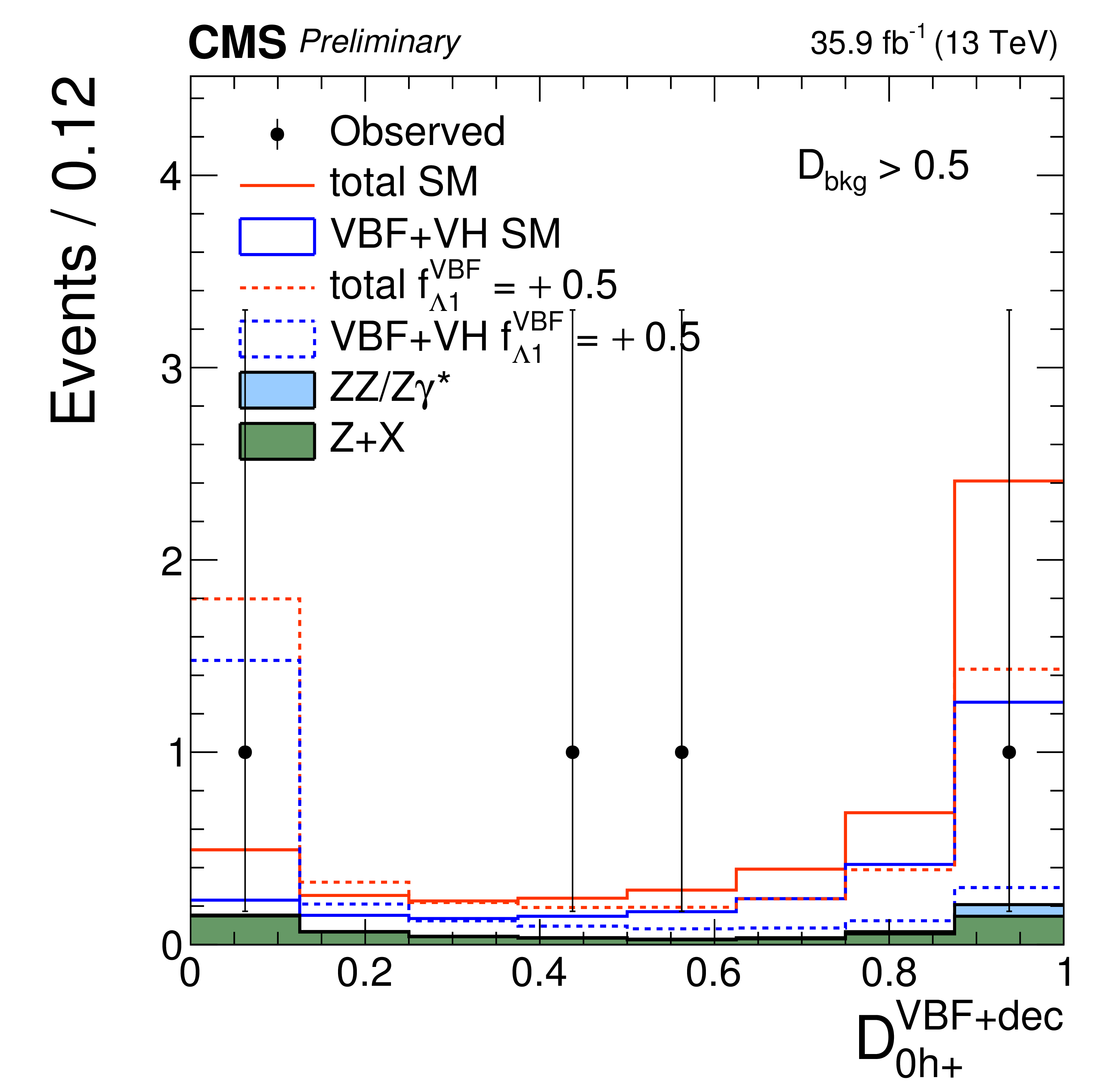
Distributions of kinematic discriminants in the $f_{\Lambda 1}$ analysis: $\mathcal {D}_{\rm bkg}$ (a), (c), (e), and $\mathcal {D}_{0h+}$ (b), (d), (f). The decay or production information used in the $\mathcal {D}_{0h+}$ discriminants is reflected in the superscript label and depends on the tagging category. Three tagging categories are shown: VBF-jets (a)-(b), $ {\mathrm {V}} \mathrm{ H } $-jets (c)-(d), and untagged (e)-(f). Points with error bars show data and histograms show expectations for background and SM or BSM signal as indicated in the legend. |

png pdf |
Additional Figure 2-a:
Distribution of the $\mathcal {D}_{\rm bkg}$ kinematic discriminant in the $f_{\Lambda 1}$ analysis. The VBF-jets tagging category is shown. Points with error bars show data and histograms show expectations for background and SM or BSM signal as indicated in the legend. |
png pdf |
Additional Figure 2-b:
Distribution of the $\mathcal {D}_{0h+}$ kinematic discriminant in the $f_{\Lambda 1}$ analysis. The decay or production information is reflected in the superscript label and depends on the tagging category. The VBF-jets tagging category is shown.Points with error bars show data and histograms show expectations for background and SM or BSM signal as indicated in the legend. |

png pdf |
Additional Figure 2-c:
Distribution of the $\mathcal {D}_{\rm bkg}$ kinematic discriminant in the $f_{\Lambda 1}$ analysis. The $ {\mathrm {V}} \mathrm{ H } $-jets tagging category is shown. Points with error bars show data and histograms show expectations for background and SM or BSM signal as indicated in the legend. |

png pdf |
Additional Figure 2-d:
Distribution of the $\mathcal {D}_{0h+}$ kinematic discriminant in the $f_{\Lambda 1}$ analysis. The decay or production information is reflected in the superscript label and depends on the tagging category. The $ {\mathrm {V}} \mathrm{ H } $-jets tagging category is shown. Points with error bars show data and histograms show expectations for background and SM or BSM signal as indicated in the legend. |
png pdf |
Additional Figure 2-e:
Distribution of the $\mathcal {D}_{\rm bkg}$ kinematic discriminant in the $f_{\Lambda 1}$ analysis. The untagged tagging category is shown. Points with error bars show data and histograms show expectations for background and SM or BSM signal as indicated in the legend. |
png pdf |
Additional Figure 2-f:
Distribution of the $\mathcal {D}_{0h+}$ kinematic discriminant in the $f_{\Lambda 1}$ analysis. The decay or production information is reflected in the superscript label and depends on the tagging category. The untagged tagging category is shown. Points with error bars show data and histograms show expectations for background and SM or BSM signal as indicated in the legend. |

png pdf |
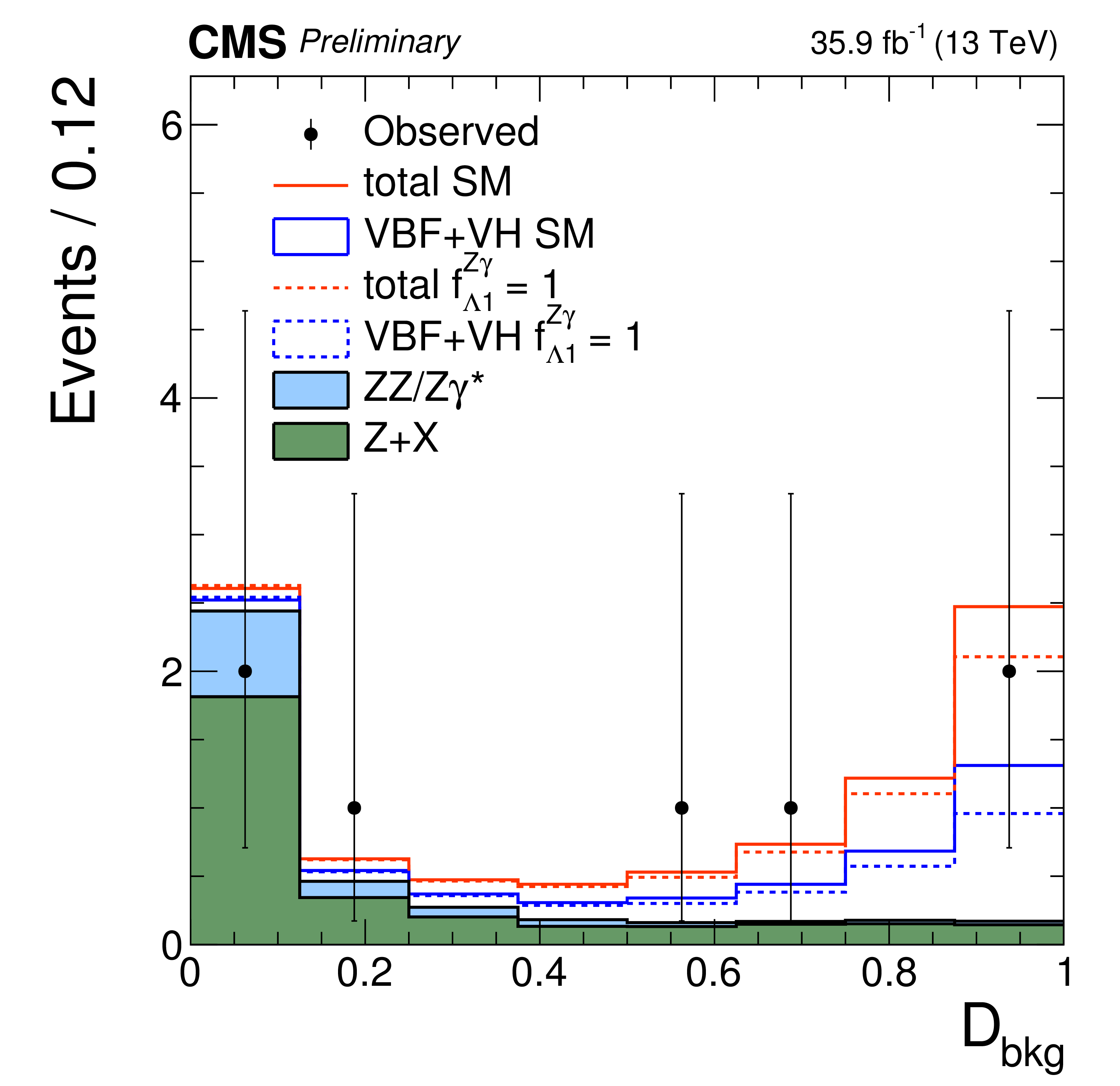
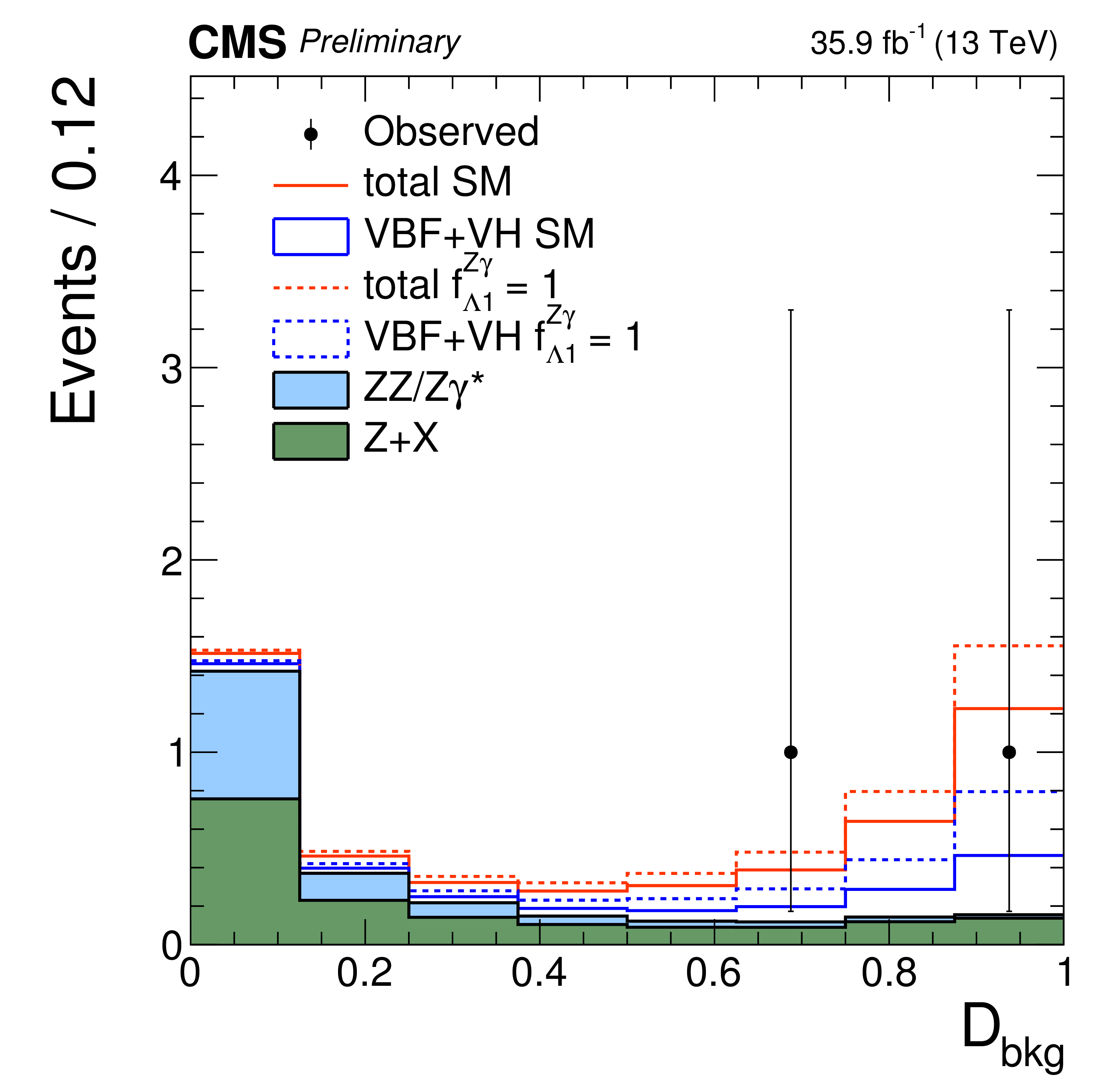
Additional Figure 3:
Distributions of kinematic discriminants in the $f_{\Lambda 1}^{{\mathrm{ Z } } \gamma }$ analysis: $\mathcal {D}_{\rm bkg}$ (a), (c), (e), and $\mathcal {D}_{0h+}$ (b), (d), (f). The decay or production information used in the $\mathcal {D}_{0h+}$ discriminants is reflected in the superscript label and depends on the tagging category. Three tagging categories are shown: VBF-jets (a)-(b), $ {\mathrm {V}} \mathrm{ H } $-jets (c)-(d), and untagged (e)-(f). Points with error bars show data and histograms show expectations for background and SM or BSM signal as indicated in the legend. |
png pdf |
Additional Figure 3-a:
Distribution of the $\mathcal {D}_{\rm bkg}$ kinematic discriminant in the $f_{\Lambda 1}^{{\mathrm{ Z } } \gamma }$ analysis.The VBF-jets tagging category is shown. Points with error bars show data and histograms show expectations for background and SM or BSM signal as indicated in the legend. |

png pdf |
Additional Figure 3-b:
Distribution of the $\mathcal {D}_{0h+}$ kinematic discriminant in the $f_{\Lambda 1}^{{\mathrm{ Z } } \gamma }$ analysis. The decay or production information is reflected in the superscript label and depends on the tagging category. The VBF-jets tagging category is shown. Points with error bars show data and histograms show expectations for background and SM or BSM signal as indicated in the legend. |
png pdf |
Additional Figure 3-c:
Distribution of the $\mathcal {D}_{\rm bkg}$ kinematic discriminant in the $f_{\Lambda 1}^{{\mathrm{ Z } } \gamma }$ analysis. The $ {\mathrm {V}} \mathrm{ H } $-jets tagging category is shown. Points with error bars show data and histograms show expectations for background and SM or BSM signal as indicated in the legend. |

png pdf |
Additional Figure 3-d:
Distribution of the $\mathcal {D}_{0h+}$ kinematic discriminant in the $f_{\Lambda 1}^{{\mathrm{ Z } } \gamma }$ analysis. The decay or production information is reflected in the superscript label and depends on the tagging category. The $ {\mathrm {V}} \mathrm{ H } $-jets tagging category is shown. Points with error bars show data and histograms show expectations for background and SM or BSM signal as indicated in the legend. |

png pdf |
Additional Figure 3-e:
Distribution of the $\mathcal {D}_{\rm bkg}$ kinematic discriminant in the $f_{\Lambda 1}^{{\mathrm{ Z } } \gamma }$ analysis. The decay or production information is reflected in the superscript label and depends on the tagging category. The untagged tagging category is shown. Points with error bars show data and histograms show expectations for background and SM or BSM signal as indicated in the legend. |
png pdf |
Additional Figure 3-f:
Distribution of the $\mathcal {D}_{0h+}$ kinematic discriminant in the $f_{\Lambda 1}^{{\mathrm{ Z } } \gamma }$ analysis. The decay or production information is reflected in the superscript label and depends on the tagging category. The untagged tagging category is shown. Points with error bars show data and histograms show expectations for background and SM or BSM signal as indicated in the legend. |
| References | ||||
| 1 | ATLAS Collaboration | Observation of a new particle in the search for the Standard Model Higgs boson with the ATLAS detector at the LHC | PLB 716 (2012) 1 | 1207.7214 |
| 2 | CMS Collaboration | Observation of a new boson at a mass of 125 GeV with the CMS experiment at the LHC | PLB716 (2012) 30--61 | CMS-HIG-12-028 1207.7235 |
| 3 | CMS Collaboration | Observation of a new boson with mass near 125 GeV in pp collisions at $ \sqrt{s} = $ 7 and 8 TeV | JHEP 06 (2013) 081 | CMS-HIG-12-036 1303.4571 |
| 4 | S. L. Glashow | Partial-symmetries of Weak Interactions | Nucl. Phys. 22 (1961) 579 | |
| 5 | F. Englert and R. Brout | Broken Symmetry and the Mass of Gauge Vector Mesons | PRL 13 (1964) 321 | |
| 6 | P. W. Higgs | Broken symmetries, massless particles and gauge fields | PL12 (1964) 132 | |
| 7 | P. W. Higgs | Broken Symmetries and the Masses of Gauge Bosons | PRL 13 (1964) 508 | |
| 8 | G. S. Guralnik, C. R. Hagen, and T. W. B. Kibble | Global Conservation Laws and Massless Particles | PRL 13 (1964) 585 | |
| 9 | S. Weinberg | A Model of Leptons | PRL 19 (1967) 1264 | |
| 10 | A. Salam | Weak and electromagnetic interactions | in Elementary particle physics: relativistic groups and analyticity, N. Svartholm, ed., 1968 Proceedings of the eighth Nobel symposium | |
| 11 | CMS Collaboration | On the mass and spin-parity of the Higgs boson candidate via its decays to Z boson pairs | PRL 110 (2013) 081803 | CMS-HIG-12-041 1212.6639 |
| 12 | CMS Collaboration | Measurement of the properties of a Higgs boson in the four-lepton final state | PRD 89 (2014) 092007 | CMS-HIG-13-002 1312.5353 |
| 13 | CMS Collaboration | Constraints on the spin-parity and anomalous HVV couplings of the Higgs boson in proton collisions at 7 and 8 TeV | PRD92 (2015), no. 1, 012004 | CMS-HIG-14-018 1411.3441 |
| 14 | ATLAS Collaboration | Evidence for the spin-0 nature of the Higgs boson using ATLAS data | PLB 726 (2013) 120 | 1307.1432 |
| 15 | ATLAS Collaboration | Study of the spin and parity of the Higgs boson in diboson decays with the ATLAS detector | EPJC75 (2015), no. 10, 476 | 1506.05669 |
| 16 | CMS Collaboration | Combined search for anomalous pseudoscalar HVV couplings in VH(H $ \to b \bar b $) production and H $ \to $ VV decay | PLB759 (2016) 672--696 | CMS-HIG-14-035 1602.04305 |
| 17 | ATLAS Collaboration | Test of CP Invariance in vector-boson fusion production of the Higgs boson using the Optimal Observable method in the ditau decay channel with the ATLAS detector | EPJC76 (2016), no. 12, 658 | 1602.04516 |
| 18 | CDF, D0 Collaboration | Tevatron Constraints on Models of the Higgs Boson with Exotic Spin and Parity Using Decays to Bottom-Antibottom Quark Pairs | PRL 114 (2015), no. 15, 151802 | 1502.00967 |
| 19 | CMS Collaboration | Limits on the Higgs boson lifetime and width from its decay to four charged leptons | PRD92 (2015), no. 7, 072010 | CMS-HIG-14-036 1507.06656 |
| 20 | C. A. Nelson | Correlation between Decay Planes in Higgs Boson Decays into $ W $ Pair (into $ Z $ Pair) | PRD 37 (1988) 1220 | |
| 21 | A. Soni and R. M. Xu | Probing CP violation via Higgs decays to four leptons | PRD 48 (1993) 5259 | hep-ph/9301225 |
| 22 | D. Chang, W.-Y. Keung, and I. Phillips | CP odd correlation in the decay of neutral Higgs boson into $ \mathrm{Z}\mathrm{Z} $, $ \mathrm{W^+}\mathrm{W^-} $, or $ \mathrm{t}\bar{\mathrm{t}} $ | PRD 48 (1993) 3225 | hep-ph/9303226 |
| 23 | V. D. Barger et al. | Higgs bosons: Intermediate mass range at e+ e- colliders | PRD 49 (1994) 79 | hep-ph/9306270 |
| 24 | T. Arens and L. M. Sehgal | Energy spectra and energy correlations in the decay H$ \to $Z Z$ \to \mu^+ \mu^- \mu^+ \mu^- $ | Z. Phys. C 66 (1995) 89 | hep-ph/9409396 |
| 25 | T. Han and J. Jiang | CP violating $ \mathrm{Z}\mathrm{Z}H $ coupling at $ \mathrm{e^+}\mathrm{e^-} $ linear colliders | PRD 63 (2001) 096007 | hep-ph/0011271 |
| 26 | T. Plehn, D. L. Rainwater, and D. Zeppenfeld | Determining the structure of Higgs couplings at the LHC | PRL 88 (2002) 051801 | hep-ph/0105325 |
| 27 | S. Y. Choi, D. J. Miller, M. M. M uhlleitner, and P. M. Zerwas | Identifying the Higgs spin and parity in decays to Z pairs | PLB 553 (2003) 61 | hep-ph/0210077 |
| 28 | C. P. Buszello, I. Fleck, P. Marquard, and J. J. van der Bij | Prospective analysis of spin- and CP-sensitive variables in $ \mathrm{H} \to \mathrm{Z}\mathrm{Z} \to l_1^+ l_1^- l_2^+ l_2^- $ at the LHC | EPJC 32 (2004) 209 | hep-ph/0212396 |
| 29 | E. Accomando et al. | Workshop on CP Studies and Non-Standard Higgs Physics | hep-ph/0608079 | |
| 30 | R. M. Godbole, D. J. Miller, and M. M. M uhlleitner | Aspects of CP violation in the H ZZ coupling at the LHC | JHEP 12 (2007) 031 | 0708.0458 |
| 31 | K. Hagiwara, Q. Li, and K. Mawatari | Jet angular correlation in vector-boson fusion processes at hadron colliders | JHEP 07 (2009) 101 | 0905.4314 |
| 32 | Y. Gao et al. | Spin determination of single-produced resonances at hadron colliders | PRD 81 (2010) 075022 | 1001.3396 |
| 33 | A. De R\' ujula et al. | Higgs look-alikes at the LHC | PRD 82 (2010) 013003 | 1001.5300 |
| 34 | N. D. Christensen, T. Han, and Y. Li | Testing CP Violation in ZZH Interactions at the LHC | PLB 693 (2010) 28 | 1005.5393 |
| 35 | J. S. Gainer, K. Kumar, I. Low, and R. Vega-Morales | Improving the sensitivity of Higgs boson searches in the golden channel | JHEP 11 (2011) 027 | 1108.2274 |
| 36 | S. Bolognesi et al. | Spin and parity of a single-produced resonance at the LHC | PRD 86 (2012) 095031 | 1208.4018 |
| 37 | J. Ellis, D. S. Hwang, V. Sanz, and T. You | A Fast Track towards the `Higgs' Spin and Parity | JHEP 11 (2012) 134 | 1208.6002 |
| 38 | Y. Chen, N. Tran, and R. Vega-Morales | Scrutinizing the Higgs Signal and Background in the $ 2\mathrm{e}2\mu $ Golden Channel | JHEP 01 (2013) 182 | 1211.1959 |
| 39 | J. S. Gainer et al. | Geolocating the Higgs Boson Candidate at the LHC | PRL 111 (2013) 041801 | 1304.4936 |
| 40 | P. Artoisenet et al. | A framework for Higgs characterisation | JHEP 11 (2013) 043 | 1306.6464 |
| 41 | I. Anderson et al. | Constraining anomalous HVV interactions at proton and lepton colliders | PRD 89 (2014) 035007 | 1309.4819 |
| 42 | M. Chen et al. | Role of interference in unraveling the ZZ couplings of the newly discovered boson at the LHC | PRD 89 (2014) 034002 | 1310.1397 |
| 43 | Y. Chen and R. Vega-Morales | Extracting Effective Higgs Couplings in the Golden Channel | JHEP 04 (2014) 057 | 1310.2893 |
| 44 | J. S. Gainer et al. | Beyond Geolocating: Constraining Higher Dimensional Operators in $ H \to 4\ell $ with Off-Shell Production and More | PRD91 (2015), no. 3, 035011 | 1403.4951 |
| 45 | M. Gonzalez-Alonso, A. Greljo, G. Isidori, and D. Marzocca | Pseudo-observables in Higgs decays | EPJC75 (2015) 128 | 1412.6038 |
| 46 | A. Greljo, G. Isidori, J. M. Lindert, and D. Marzocca | Pseudo-observables in electroweak Higgs production | EPJC76 (2016), no. 3, 158 | 1512.06135 |
| 47 | A. V. Gritsan, R. Roentsch, M. Schulze, and M. Xiao | Constraining anomalous Higgs boson couplings to the heavy flavor fermions using matrix element techniques | PRD94 (2016), no. 5, 055023 | 1606.03107 |
| 48 | N. Kauer and G. Passarino | Inadequacy of zero-width approximation for a light Higgs boson signal | JHEP 08 (2012) 116 | 1206.4803 |
| 49 | F. Caola and K. Melnikov | Constraining the Higgs boson width with $ ZZ $ production at the LHC | PRD 88 (2013) 054024 | 1307.4935 |
| 50 | CMS Collaboration | Constraints on the Higgs boson width from off-shell production and decay to Z-boson pairs | PLB 736 (2014) 64 | CMS-HIG-14-002 1405.3455 |
| 51 | CMS Collaboration | The CMS experiment at the CERN LHC | JINST 3 (2008) S08004 | CMS-00-001 |
| 52 | S. Frixione, P. Nason, and C. Oleari | Matching NLO QCD computations with Parton Shower simulations: the POWHEG method | JHEP 11 (2007) 070 | 0709.2092 |
| 53 | E. Bagnaschi, G. Degrassi, P. Slavich, and A. Vicini | Higgs production via gluon fusion in the POWHEG approach in the SM and in the MSSM | JHEP 02 (2012) 088 | 1111.2854 |
| 54 | P. Nason and C. Oleari | NLO Higgs boson production via vector-boson fusion matched with shower in POWHEG | JHEP 02 (2010) 037 | 0911.5299 |
| 55 | J. M. Campbell and R. K. Ellis | MCFM for the Tevatron and the LHC | NPPS 205 (2010) 10 | 1007.3492 |
| 56 | J. M. Campbell, R. K. Ellis, and C. Williams | Vector boson pair production at the LHC | JHEP 07 (2011) 018 | 1105.0020 |
| 57 | J. M. Campbell, R. K. Ellis, and C. Williams | Bounding the Higgs width at the LHC using full analytic results for $ \mathrm{g}\mathrm{g}\to \mathrm{e^-}\mathrm{e^+} \mu^- \mu^+ $ | JHEP 04 (2014) 060 | 1311.3589 |
| 58 | S. Jadach, J. H. Kuhn, and Z. Was | TAUOLA - a library of Monte Carlo programs to simulate decays of polarized tau leptons | Comput. Phys. Comm. 64 (1991) 275 | |
| 59 | NNPDF Collaboration | Unbiased global determination of parton distributions and their uncertainties at NNLO and at LO | Nucl. Phys. B855 (2012) 153--221 | 1107.2652 |
| 60 | T. Sjjostrand et al. | An introduction to PYTHIA 8.2 | Computer Physics Communications 191 (2015) 159 | |
| 61 | GEANT4 Collaboration | GEANT4---a simulation toolkit | NIMA 506 (2003) 250 | |
| 62 | CMS Collaboration | Higgs to 4 leptons with 13 TeV with full 2016 dataset | CMS Note HIG-16-041 | |
| 63 | CMS Collaboration | Performance of CMS muon reconstruction in pp collision events at $ \sqrt{s} = $ 7 TeV | JINST 7 (2012) P10002 | CMS-MUO-10-004 1206.4071 |
| 64 | M. Cacciari, G. P. Salam, and G. Soyez | The anti-$ k_t $ jet clustering algorithm | JHEP 04 (2008) 063 | 0802.1189 |
| 65 | M. Cacciari, G. P. Salam, and G. Soyez | FastJet user manual | EPJC 72 (2012) 1896 | 1111.6097 |
| 66 | CMS Collaboration | Determination of Jet Energy Calibration and Transverse Momentum Resolution in CMS | JINST 6 (2011) P11002 | CMS-JME-10-011 1107.4277 |
| 67 | M. Rosenblatt | Remarks on Some Nonparametric Estimates of a Density Function | Ann. Math. Stat. 27 (1956) 832 | |
| 68 | E. Parzen | On Estimation of a Probability Density Function and Mode | Ann. Math. Stat. 33 (1962) 1065 | |
| 69 | S. S. Wilks | The Large-Sample Distribution of the Likelihood Ratio for Testing Composite Hypotheses | Ann. Math. Stat. 9 (1938) 60 | |
|
|
Compact Muon Solenoid LHC, CERN |
|

|

|

|

|

|