

Compact Muon Solenoid
LHC, CERN
| CMS-PAS-FSQ-15-009 | ||
| Femtoscopic Bose-Einstein correlations of charged hadrons in proton-proton collisions at $\sqrt{s}= $ 13 TeV | ||
| CMS Collaboration | ||
| May 2018 | ||
| Abstract: Femtoscopic correlations between charged hadrons are measured over a broad multiplicity range, from a few particles up to about 250 reconstructed charged hadrons, in proton-proton collisions at $\sqrt{s}= $ 13 TeV. The results are based on data collected by the CMS detector at the CERN LHC. Three methods with different dependencies on simulations, when extracting and fitting the correlation functions, are compared and are found to give consistent results. The measured lengths of homogeneity are studied as functions of particle multiplicity and pair transverse mass. The results are compared with those from lower energies and other experiments, as well as with theoretical predictions. | ||
|
Links:
CDS record (PDF) ;
CADI line (restricted) ;
These preliminary results are superseded in this paper, JHEP 03 (2020) 014. The superseded preliminary plots can be found here. |
||
| Figures | |

png pdf |
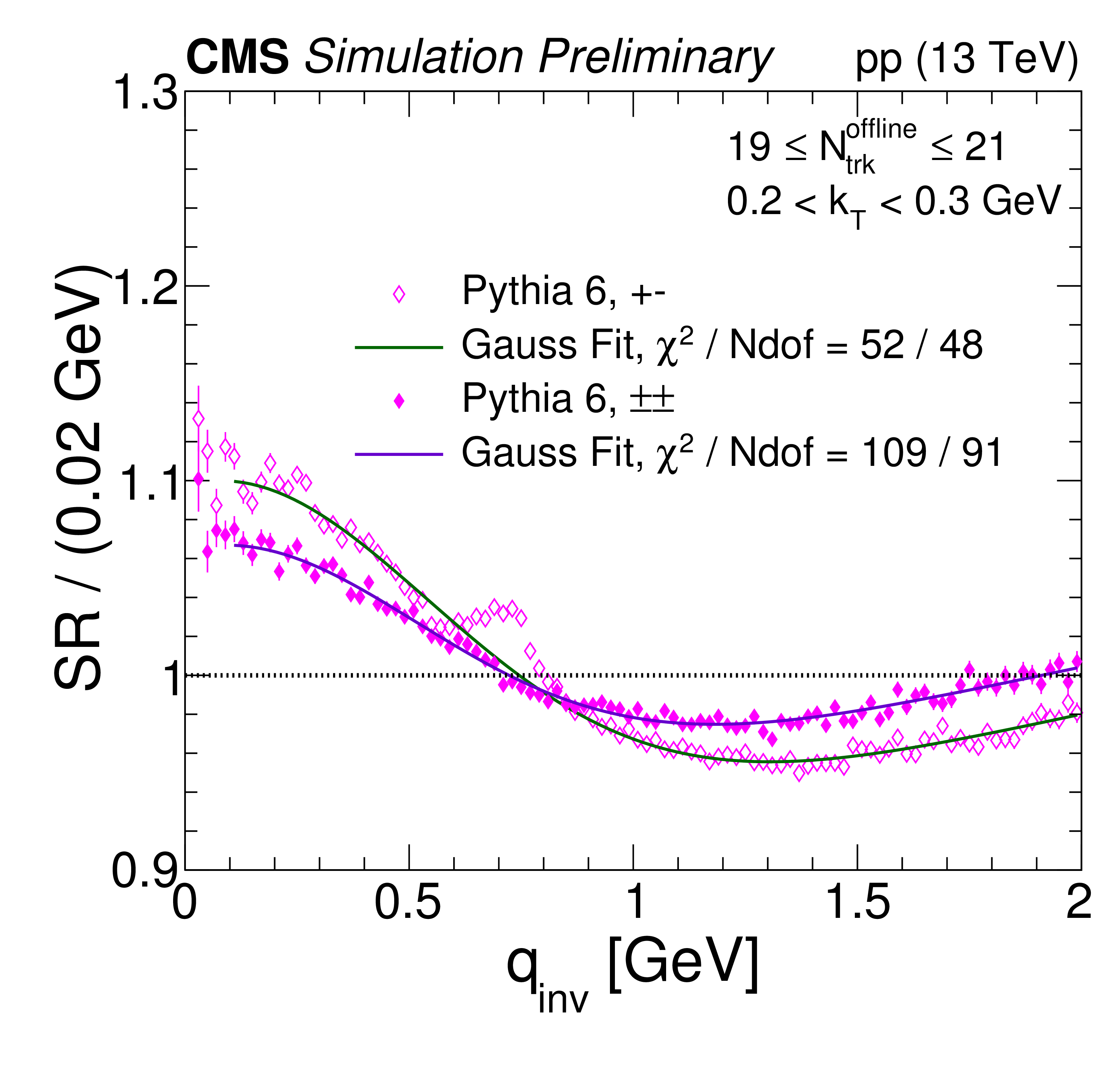
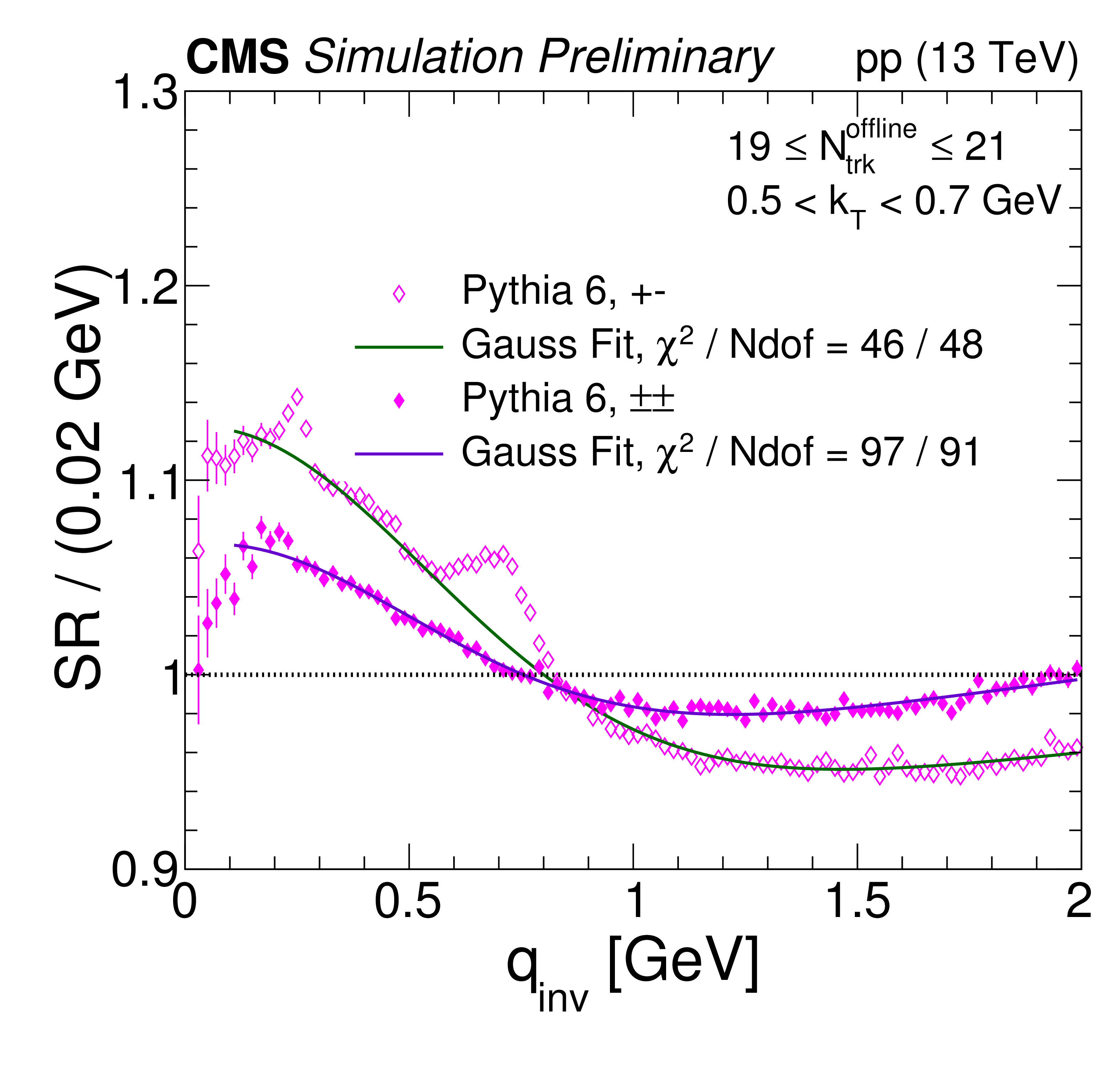
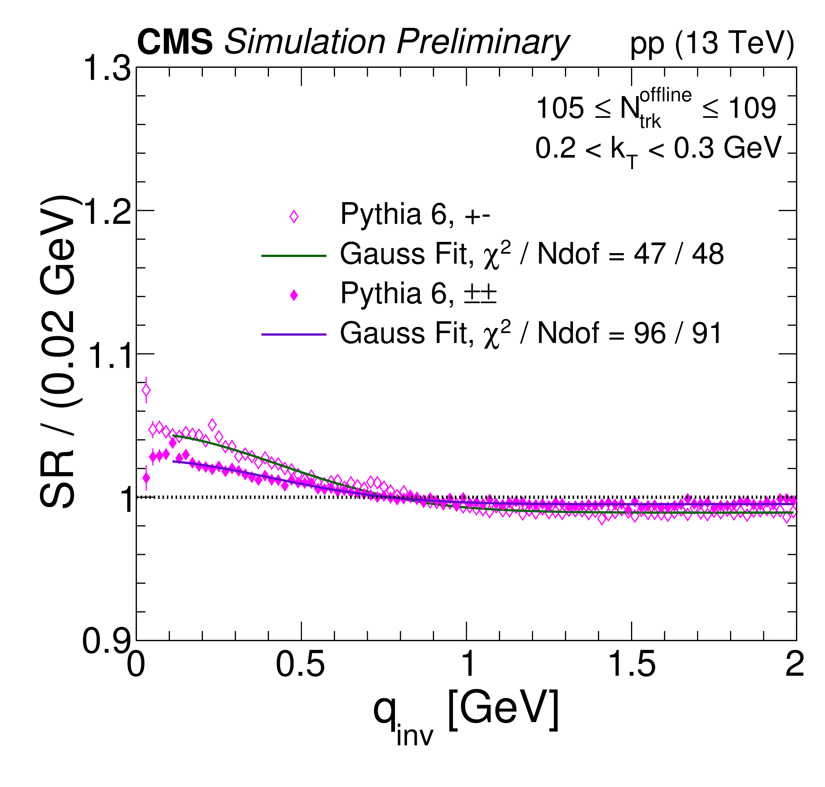
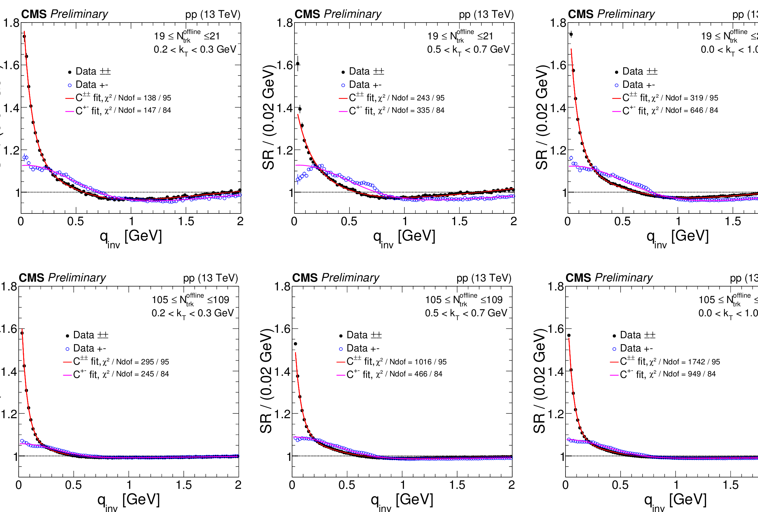
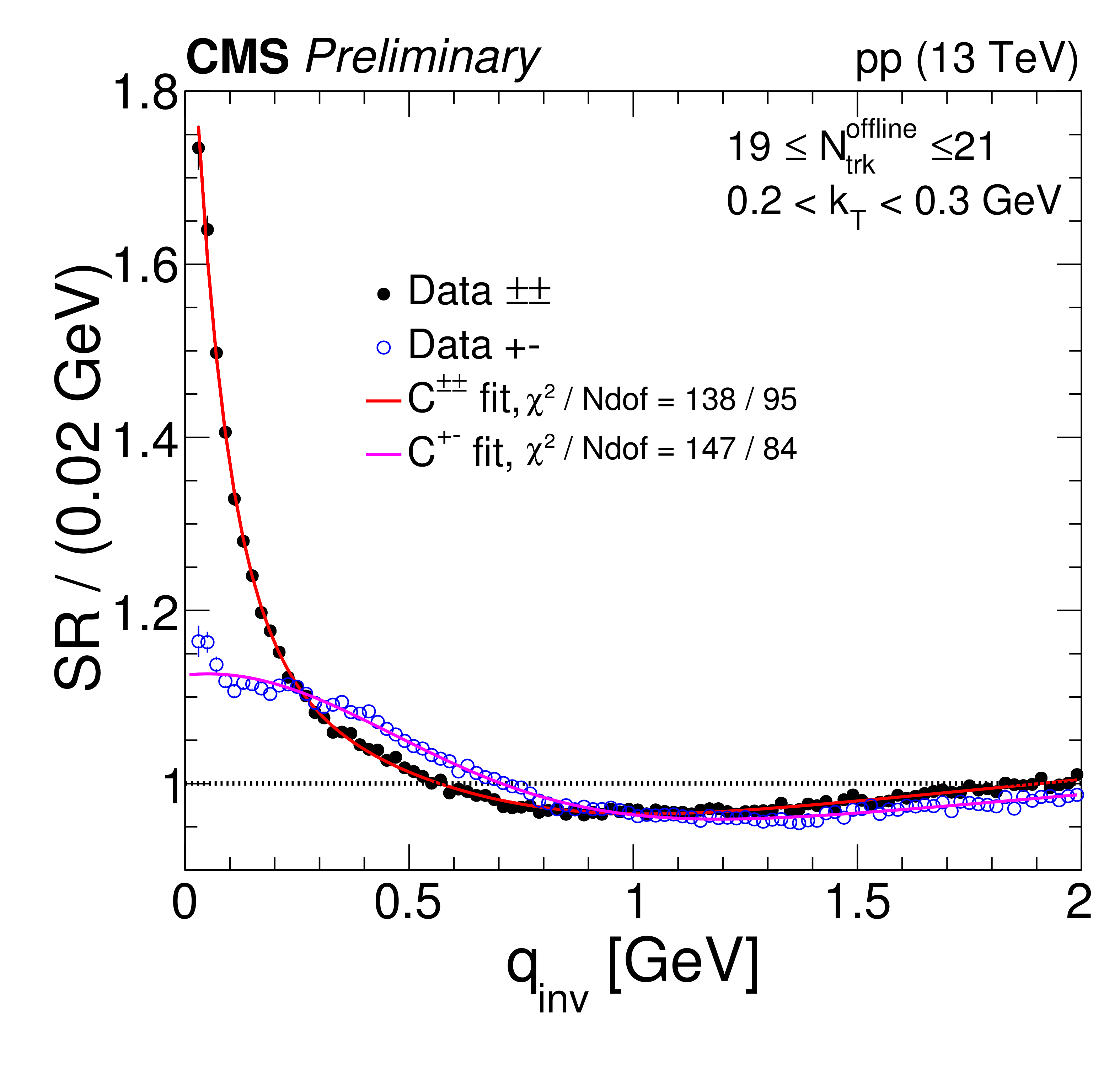
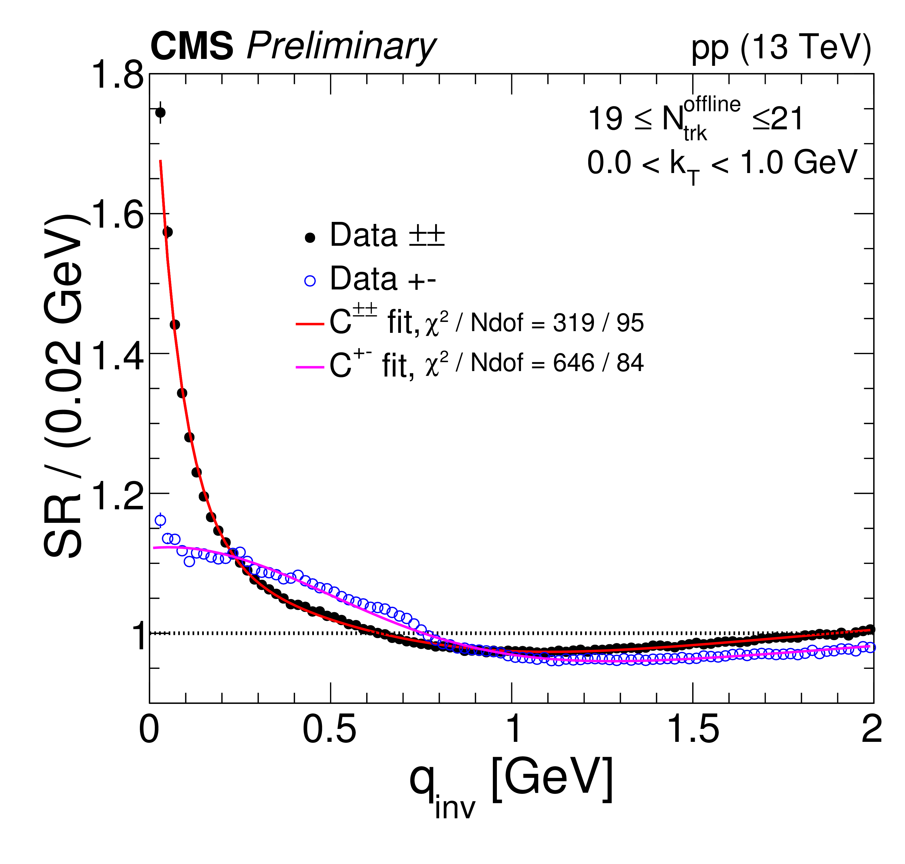
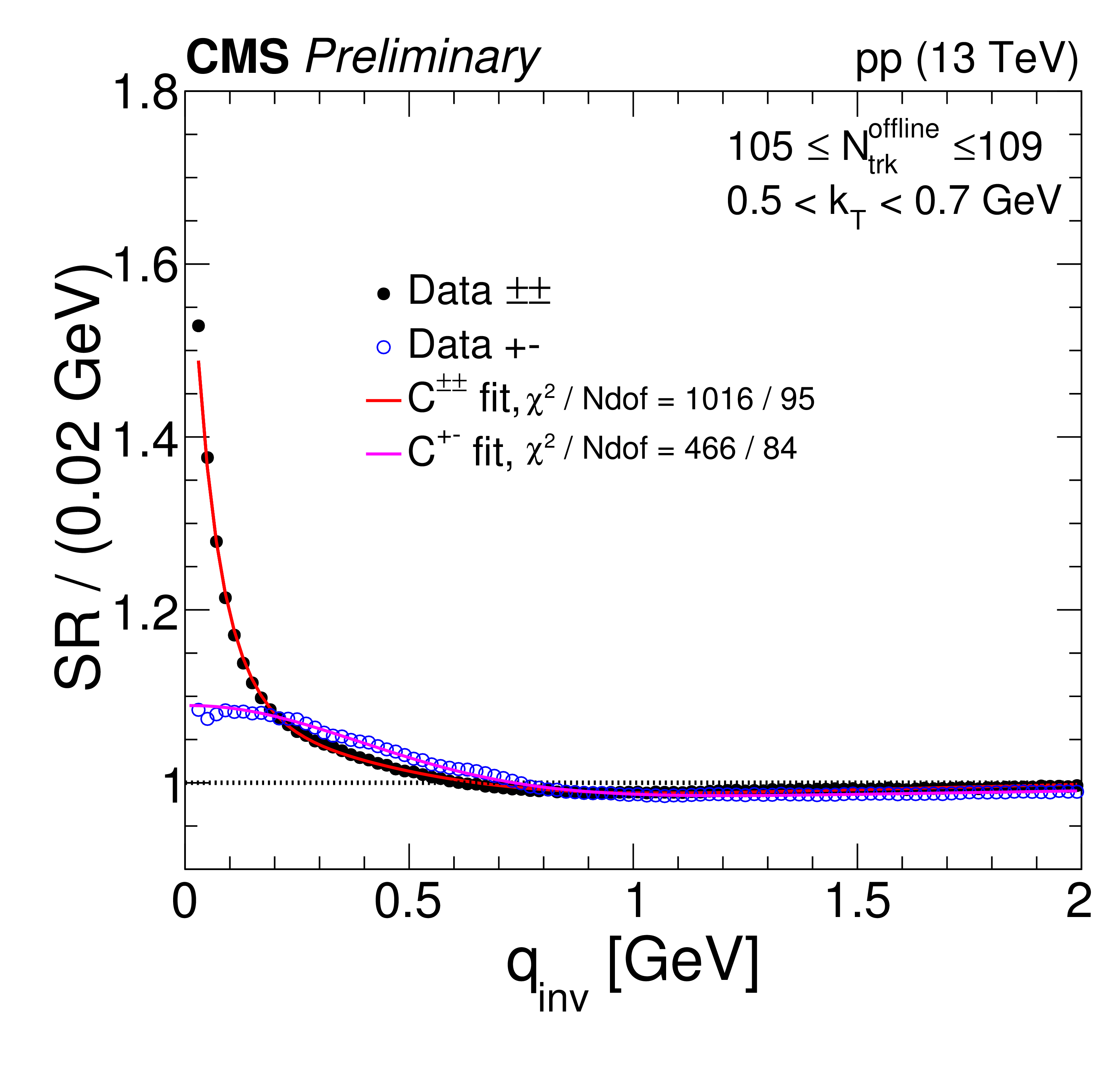
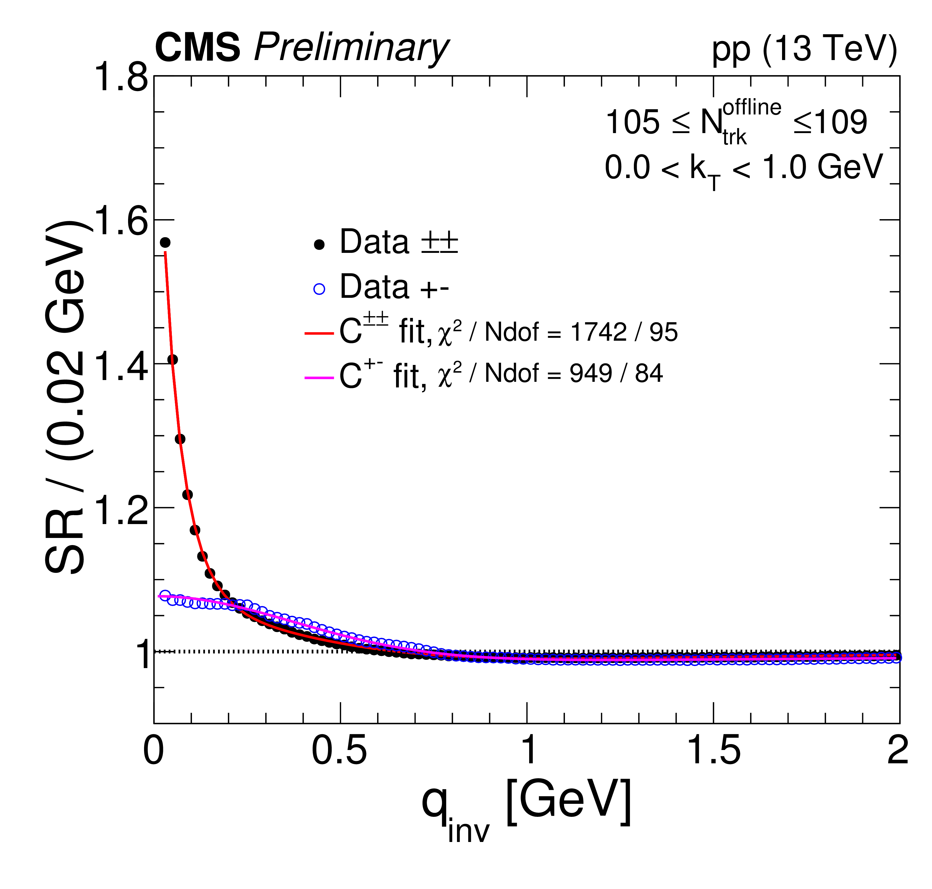
Figure 1:
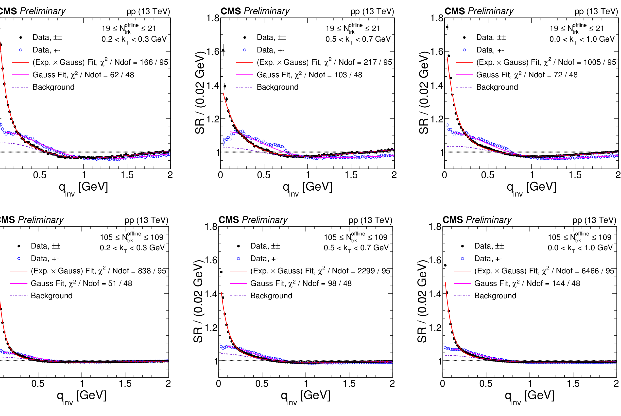
Same-sign and opposite-sign SR employing PYTHIA6 (Z2*) in different bins of $N^\text {offline}_\text {track}$ and $ {k_{\mathrm {T}}} $ with the respective Gaussian fit from Equation (4). The following $ {q_\text {inv}} $ ranges are excluded from the fits: 0.2 $ < {q_\text {inv}} < $ 0.3 GeV, 0.4 $ < {q_\text {inv}} < $ 0.9 GeV and 0.95 $ < {q_\text {inv}} < $ 1.2 GeV. Coulomb interactions are not included in the simulation. |
png pdf |
Figure 1-a:
Same-sign and opposite-sign SR employing PYTHIA6 (Z2*) in different bins of $N^\text {offline}_\text {track}$ and $ {k_{\mathrm {T}}} $ with the respective Gaussian fit from Equation (4). The following $ {q_\text {inv}} $ ranges are excluded from the fits: 0.2 $ < {q_\text {inv}} < $ 0.3 GeV, 0.4 $ < {q_\text {inv}} < $ 0.9 GeV and 0.95 $ < {q_\text {inv}} < $ 1.2 GeV. Coulomb interactions are not included in the simulation. |
png pdf |
Figure 1-b:
Same-sign and opposite-sign SR employing PYTHIA6 (Z2*) in different bins of $N^\text {offline}_\text {track}$ and $ {k_{\mathrm {T}}} $ with the respective Gaussian fit from Equation (4). The following $ {q_\text {inv}} $ ranges are excluded from the fits: 0.2 $ < {q_\text {inv}} < $ 0.3 GeV, 0.4 $ < {q_\text {inv}} < $ 0.9 GeV and 0.95 $ < {q_\text {inv}} < $ 1.2 GeV. Coulomb interactions are not included in the simulation. |

png pdf |
Figure 1-c:
Same-sign and opposite-sign SR employing PYTHIA6 (Z2*) in different bins of $N^\text {offline}_\text {track}$ and $ {k_{\mathrm {T}}} $ with the respective Gaussian fit from Equation (4). The following $ {q_\text {inv}} $ ranges are excluded from the fits: 0.2 $ < {q_\text {inv}} < $ 0.3 GeV, 0.4 $ < {q_\text {inv}} < $ 0.9 GeV and 0.95 $ < {q_\text {inv}} < $ 1.2 GeV. Coulomb interactions are not included in the simulation. |
png pdf |
Figure 1-d:
Same-sign and opposite-sign SR employing PYTHIA6 (Z2*) in different bins of $N^\text {offline}_\text {track}$ and $ {k_{\mathrm {T}}} $ with the respective Gaussian fit from Equation (4). The following $ {q_\text {inv}} $ ranges are excluded from the fits: 0.2 $ < {q_\text {inv}} < $ 0.3 GeV, 0.4 $ < {q_\text {inv}} < $ 0.9 GeV and 0.95 $ < {q_\text {inv}} < $ 1.2 GeV. Coulomb interactions are not included in the simulation. |

png pdf |
Figure 1-e:
Same-sign and opposite-sign SR employing PYTHIA6 (Z2*) in different bins of $N^\text {offline}_\text {track}$ and $ {k_{\mathrm {T}}} $ with the respective Gaussian fit from Equation (4). The following $ {q_\text {inv}} $ ranges are excluded from the fits: 0.2 $ < {q_\text {inv}} < $ 0.3 GeV, 0.4 $ < {q_\text {inv}} < $ 0.9 GeV and 0.95 $ < {q_\text {inv}} < $ 1.2 GeV. Coulomb interactions are not included in the simulation. |

png pdf |
Figure 1-f:
Same-sign and opposite-sign SR employing PYTHIA6 (Z2*) in different bins of $N^\text {offline}_\text {track}$ and $ {k_{\mathrm {T}}} $ with the respective Gaussian fit from Equation (4). The following $ {q_\text {inv}} $ ranges are excluded from the fits: 0.2 $ < {q_\text {inv}} < $ 0.3 GeV, 0.4 $ < {q_\text {inv}} < $ 0.9 GeV and 0.95 $ < {q_\text {inv}} < $ 1.2 GeV. Coulomb interactions are not included in the simulation. |
png pdf |
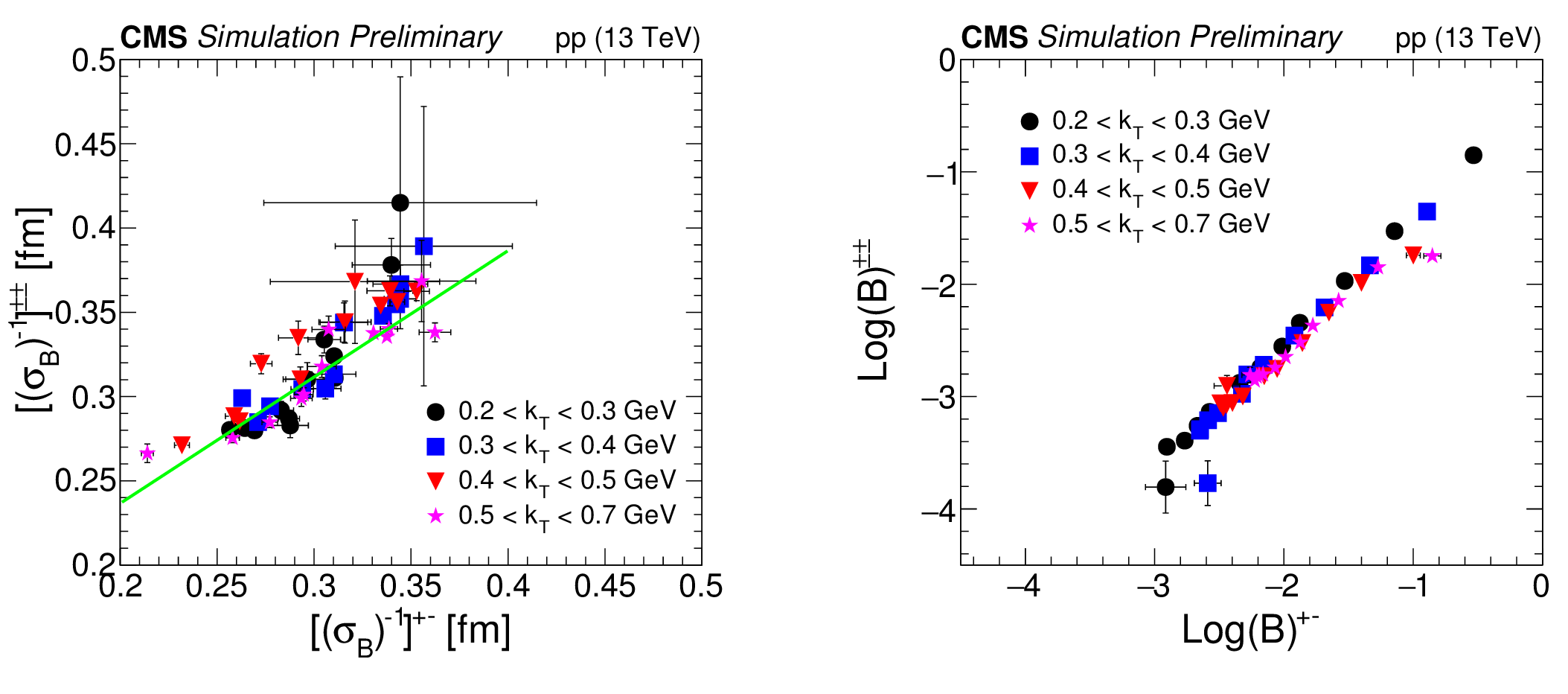
Figure 2:
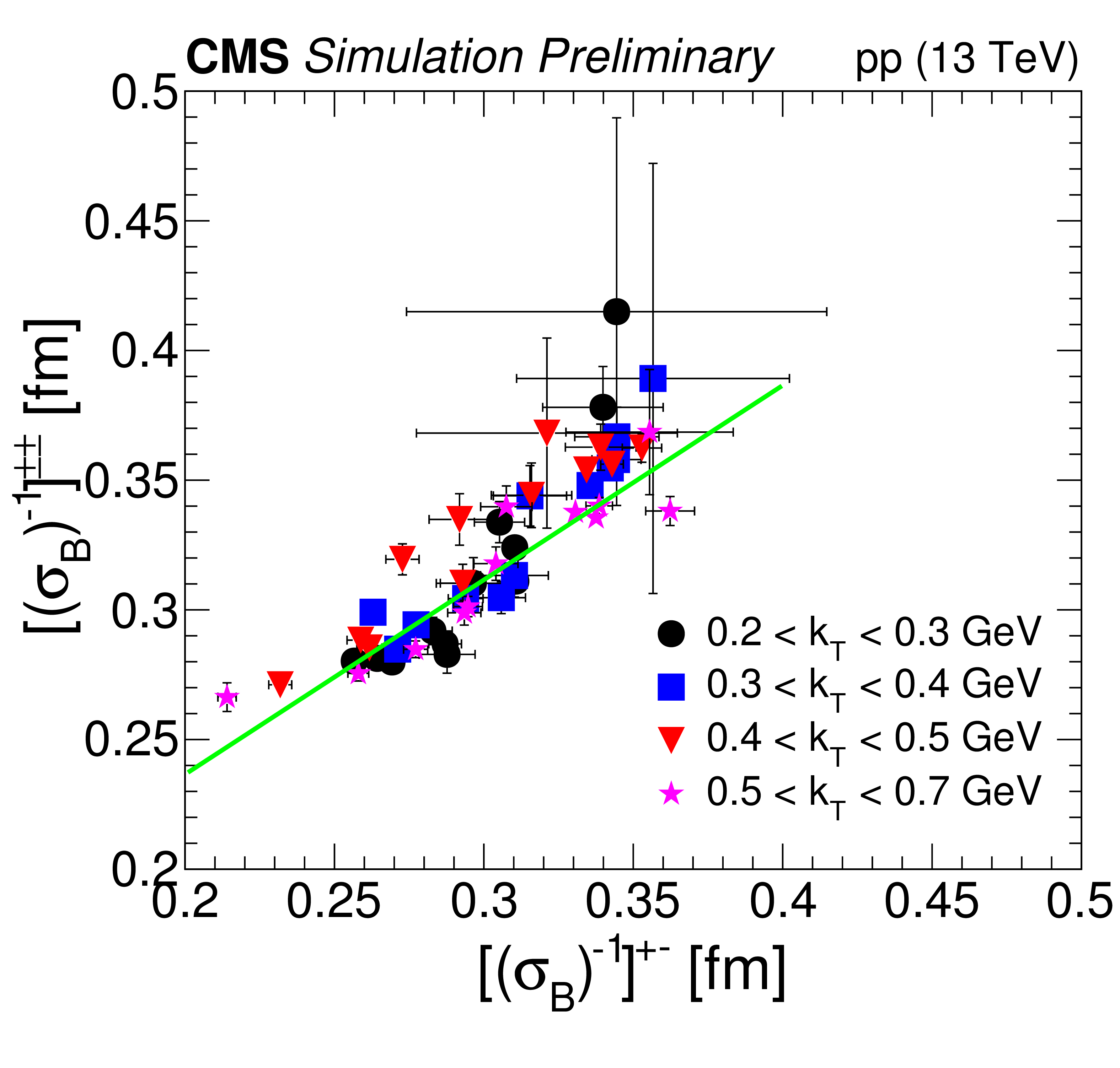
Relations between same- and opposite-sign fit parameters from Eq. (4), as a function of $ {k_{\mathrm {T}}} $ and $N^\text {offline}_\text {track}$ for events in MB (i.e., higher $(\sigma _{B})^{-1}$ and lower $\text {Log}(B)$) and HM (i.e., lower $(\sigma _{B})^{-1}$ and higher $\text {Log}(B)$) ranges. For a given $ {k_{\mathrm {T}}} $ range, each point represents an $N^\text {offline}_\text {track}$ bin. The line in the left plot is the fit to all the data. |
png pdf |
Figure 2-a:
Relations between same- and opposite-sign fit parameters from Eq. (4), as a function of $ {k_{\mathrm {T}}} $ and $N^\text {offline}_\text {track}$ for events in MB (i.e., higher $(\sigma _{B})^{-1}$ and lower $\text {Log}(B)$) and HM (i.e., lower $(\sigma _{B})^{-1}$ and higher $\text {Log}(B)$) ranges. For a given $ {k_{\mathrm {T}}} $ range, each point represents an $N^\text {offline}_\text {track}$ bin. The line in the left plot is the fit to all the data. |

png pdf |
Figure 2-b:
Relations between same- and opposite-sign fit parameters from Eq. (4), as a function of $ {k_{\mathrm {T}}} $ and $N^\text {offline}_\text {track}$ for events in MB (i.e., higher $(\sigma _{B})^{-1}$ and lower $\text {Log}(B)$) and HM (i.e., lower $(\sigma _{B})^{-1}$ and higher $\text {Log}(B)$) ranges. For a given $ {k_{\mathrm {T}}} $ range, each point represents an $N^\text {offline}_\text {track}$ bin. The line in the left plot is the fit to all the data. |
png pdf |
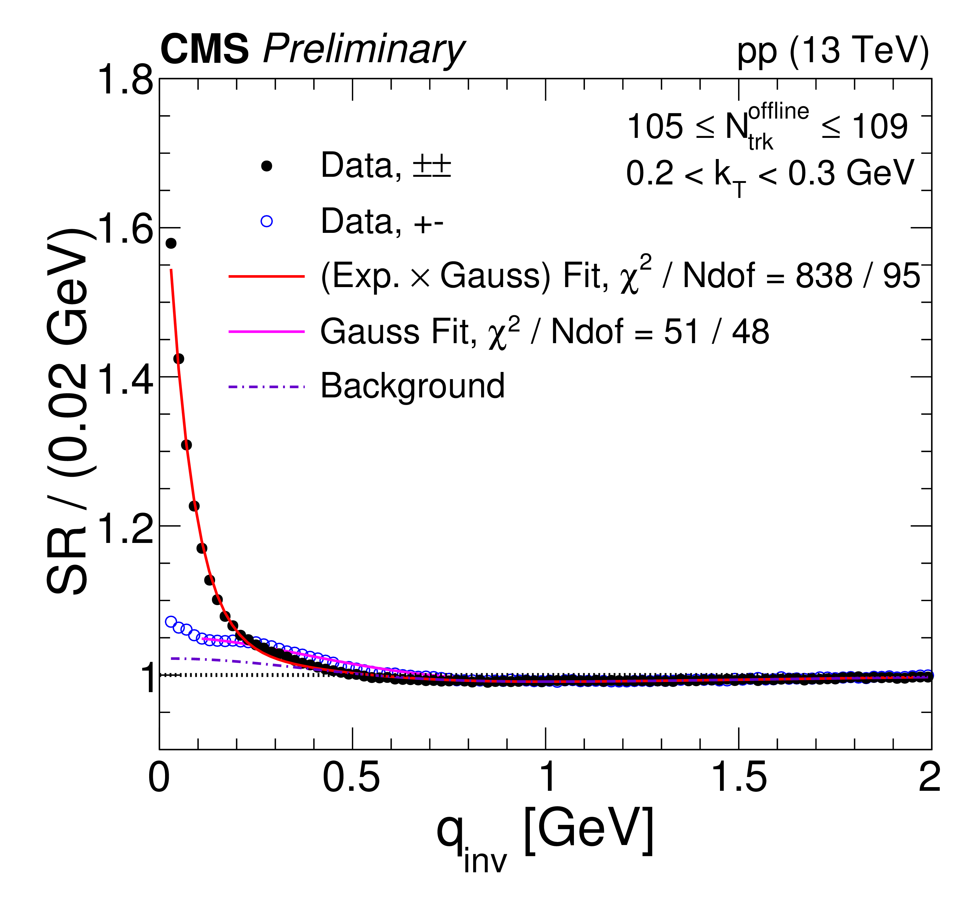
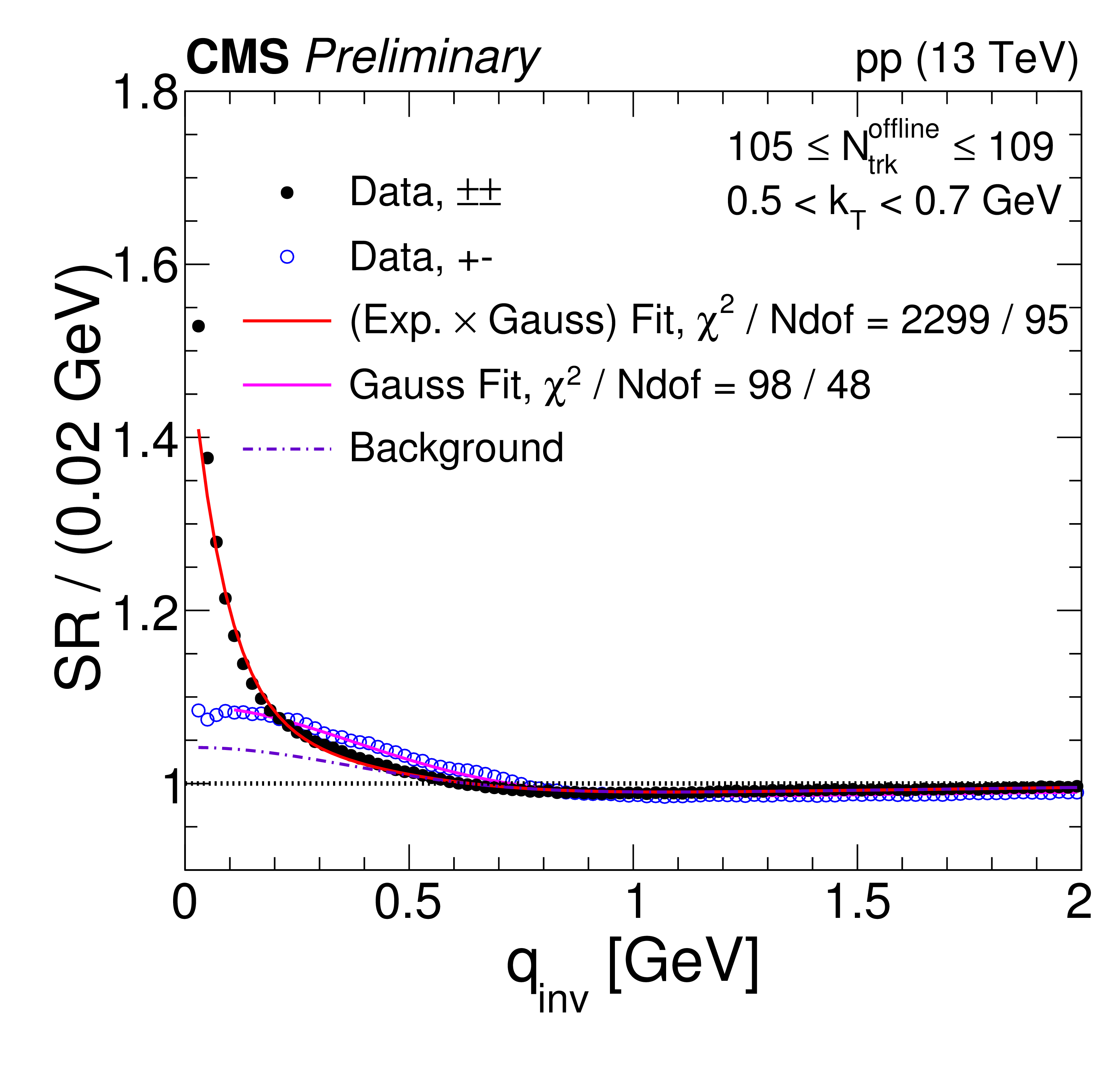
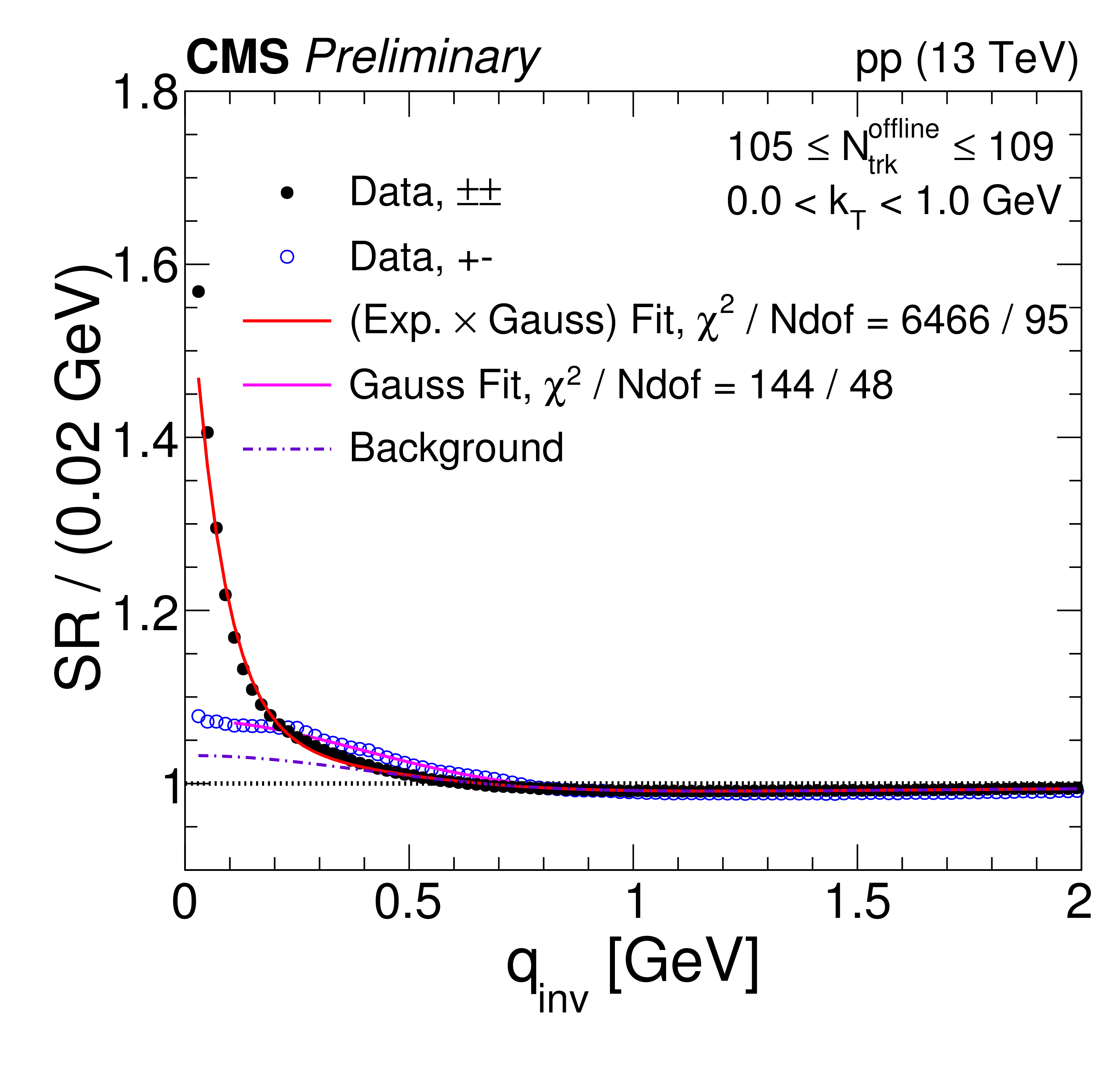
Figure 3:
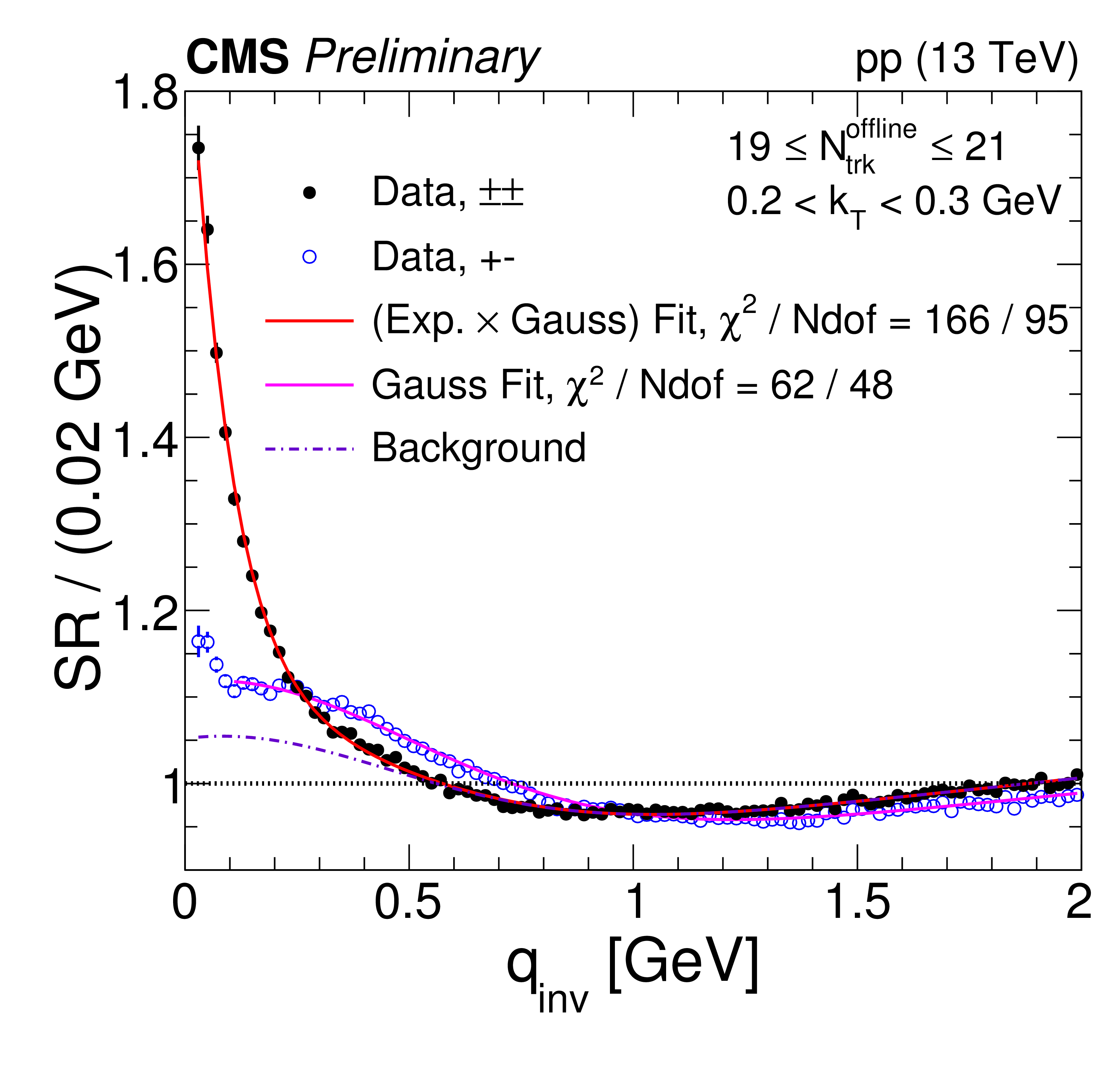
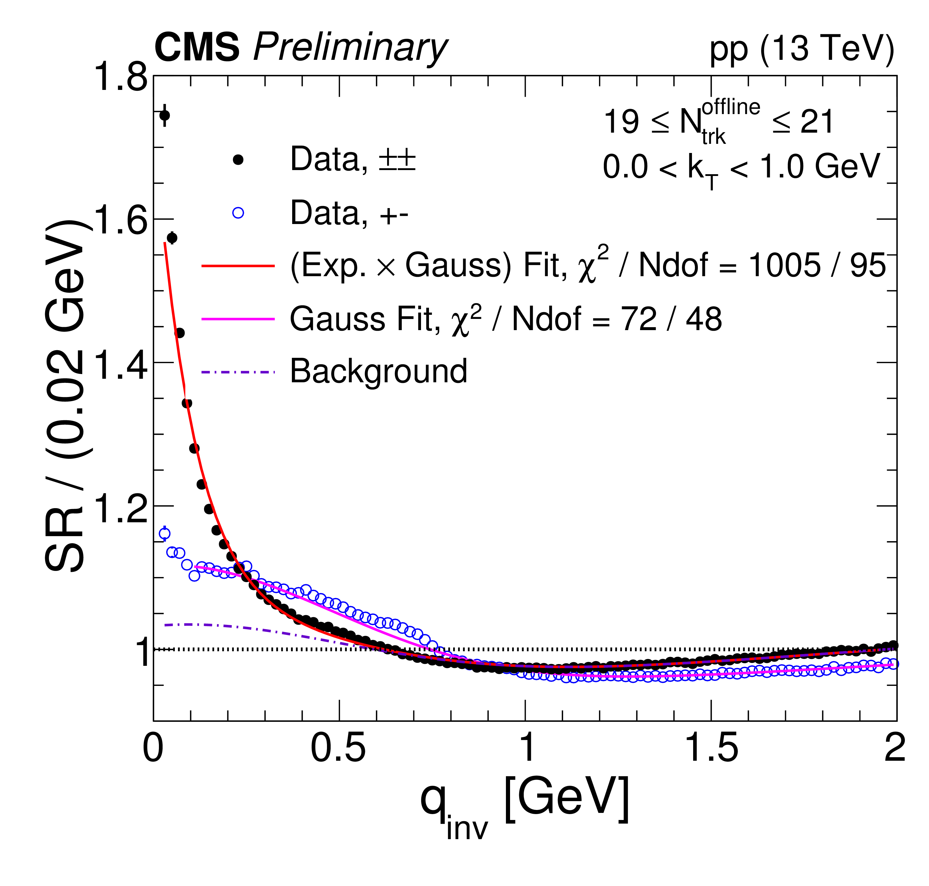
Same-sign and opposite-sign single ratios in data for different bins of $N^\text {offline}_\text {track}$ and $ {k_{\mathrm {T}}} $, with their respective fits. The label "(Exp. $\times $ Gauss) Fit'' refers to the same-sign data and is given by Eq. (7). The label "Gauss Fit'' corresponds to Eq. (4) applied to opposite-sign data and "Background'' is the component of Eq. (7) that is found from Gauss Fit by using Eqs. (5) and (6) to convert the fit parameters. Coulomb corrections are accounted for using the Gamow factor. |
png pdf |
Figure 3-a:
Same-sign and opposite-sign single ratios in data for different bins of $N^\text {offline}_\text {track}$ and $ {k_{\mathrm {T}}} $, with their respective fits. The label "(Exp. $\times $ Gauss) Fit'' refers to the same-sign data and is given by Eq. (7). The label "Gauss Fit'' corresponds to Eq. (4) applied to opposite-sign data and "Background'' is the component of Eq. (7) that is found from Gauss Fit by using Eqs. (5) and (6) to convert the fit parameters. Coulomb corrections are accounted for using the Gamow factor. |

png pdf |
Figure 3-b:
Same-sign and opposite-sign single ratios in data for different bins of $N^\text {offline}_\text {track}$ and $ {k_{\mathrm {T}}} $, with their respective fits. The label "(Exp. $\times $ Gauss) Fit'' refers to the same-sign data and is given by Eq. (7). The label "Gauss Fit'' corresponds to Eq. (4) applied to opposite-sign data and "Background'' is the component of Eq. (7) that is found from Gauss Fit by using Eqs. (5) and (6) to convert the fit parameters. Coulomb corrections are accounted for using the Gamow factor. |
png pdf |
Figure 3-c:
Same-sign and opposite-sign single ratios in data for different bins of $N^\text {offline}_\text {track}$ and $ {k_{\mathrm {T}}} $, with their respective fits. The label "(Exp. $\times $ Gauss) Fit'' refers to the same-sign data and is given by Eq. (7). The label "Gauss Fit'' corresponds to Eq. (4) applied to opposite-sign data and "Background'' is the component of Eq. (7) that is found from Gauss Fit by using Eqs. (5) and (6) to convert the fit parameters. Coulomb corrections are accounted for using the Gamow factor. |
png pdf |
Figure 3-d:
Same-sign and opposite-sign single ratios in data for different bins of $N^\text {offline}_\text {track}$ and $ {k_{\mathrm {T}}} $, with their respective fits. The label "(Exp. $\times $ Gauss) Fit'' refers to the same-sign data and is given by Eq. (7). The label "Gauss Fit'' corresponds to Eq. (4) applied to opposite-sign data and "Background'' is the component of Eq. (7) that is found from Gauss Fit by using Eqs. (5) and (6) to convert the fit parameters. Coulomb corrections are accounted for using the Gamow factor. |
png pdf |
Figure 3-e:
Same-sign and opposite-sign single ratios in data for different bins of $N^\text {offline}_\text {track}$ and $ {k_{\mathrm {T}}} $, with their respective fits. The label "(Exp. $\times $ Gauss) Fit'' refers to the same-sign data and is given by Eq. (7). The label "Gauss Fit'' corresponds to Eq. (4) applied to opposite-sign data and "Background'' is the component of Eq. (7) that is found from Gauss Fit by using Eqs. (5) and (6) to convert the fit parameters. Coulomb corrections are accounted for using the Gamow factor. |
png pdf |
Figure 3-f:
Same-sign and opposite-sign single ratios in data for different bins of $N^\text {offline}_\text {track}$ and $ {k_{\mathrm {T}}} $, with their respective fits. The label "(Exp. $\times $ Gauss) Fit'' refers to the same-sign data and is given by Eq. (7). The label "Gauss Fit'' corresponds to Eq. (4) applied to opposite-sign data and "Background'' is the component of Eq. (7) that is found from Gauss Fit by using Eqs. (5) and (6) to convert the fit parameters. Coulomb corrections are accounted for using the Gamow factor. |

png pdf |
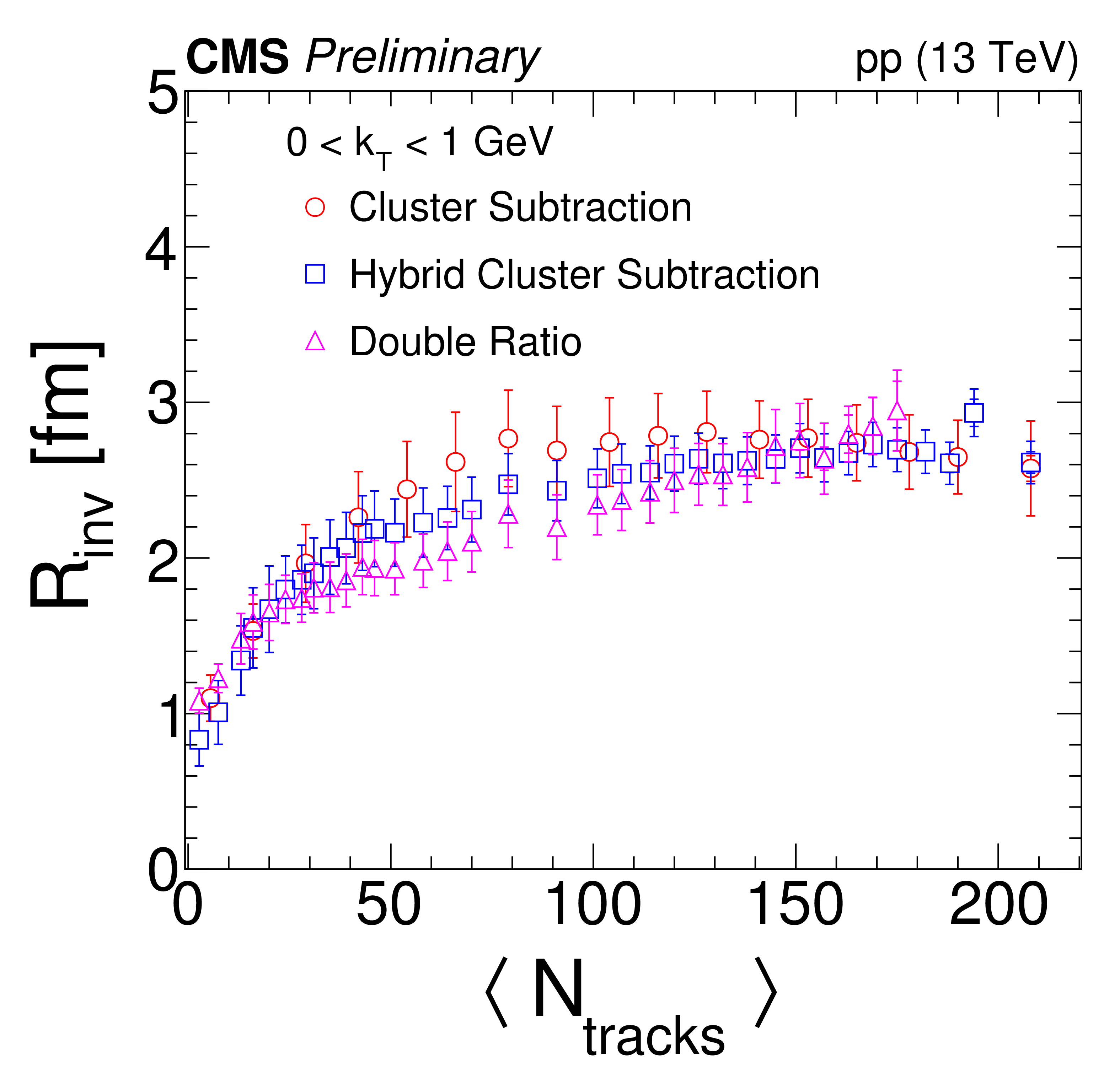
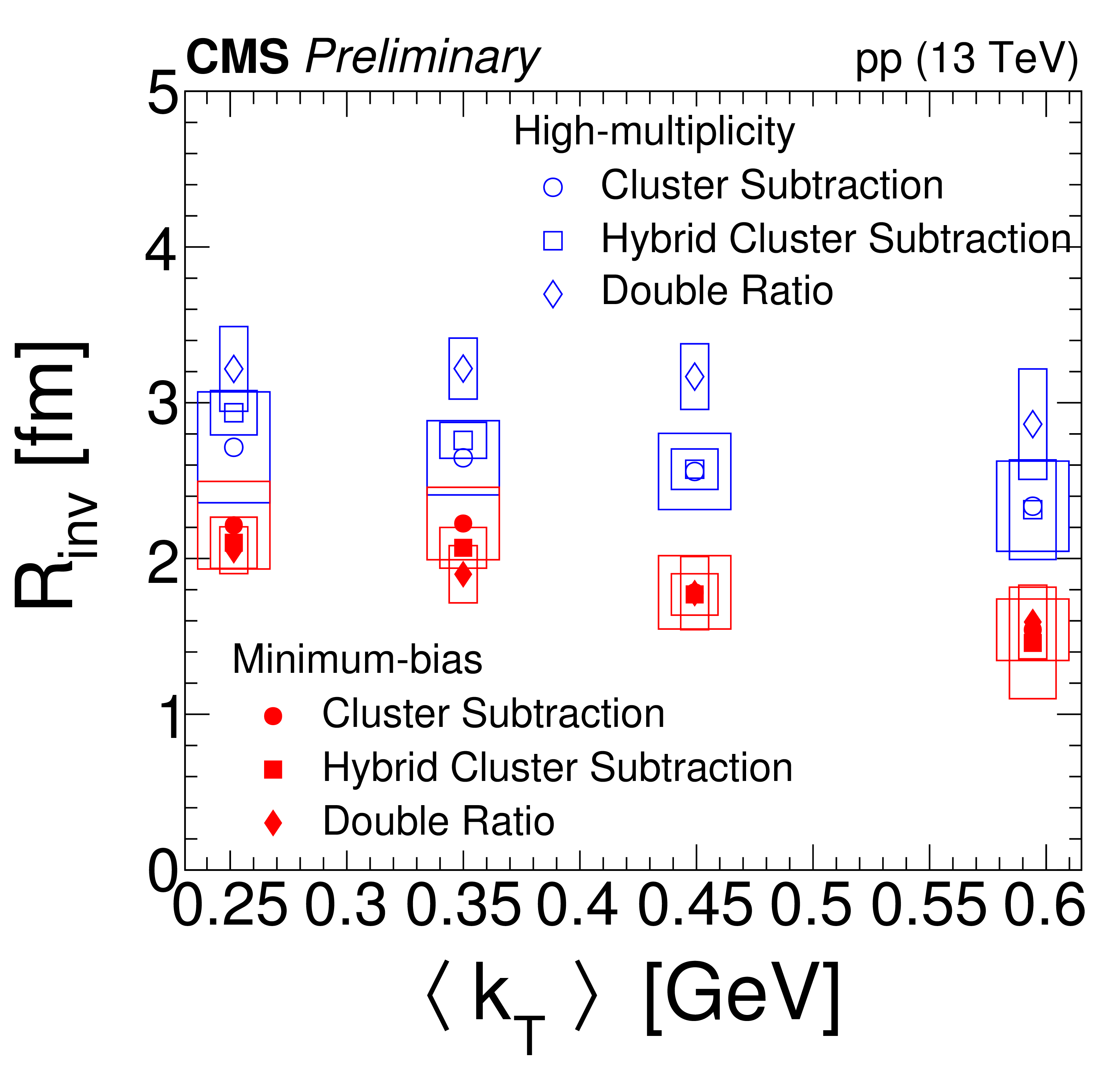
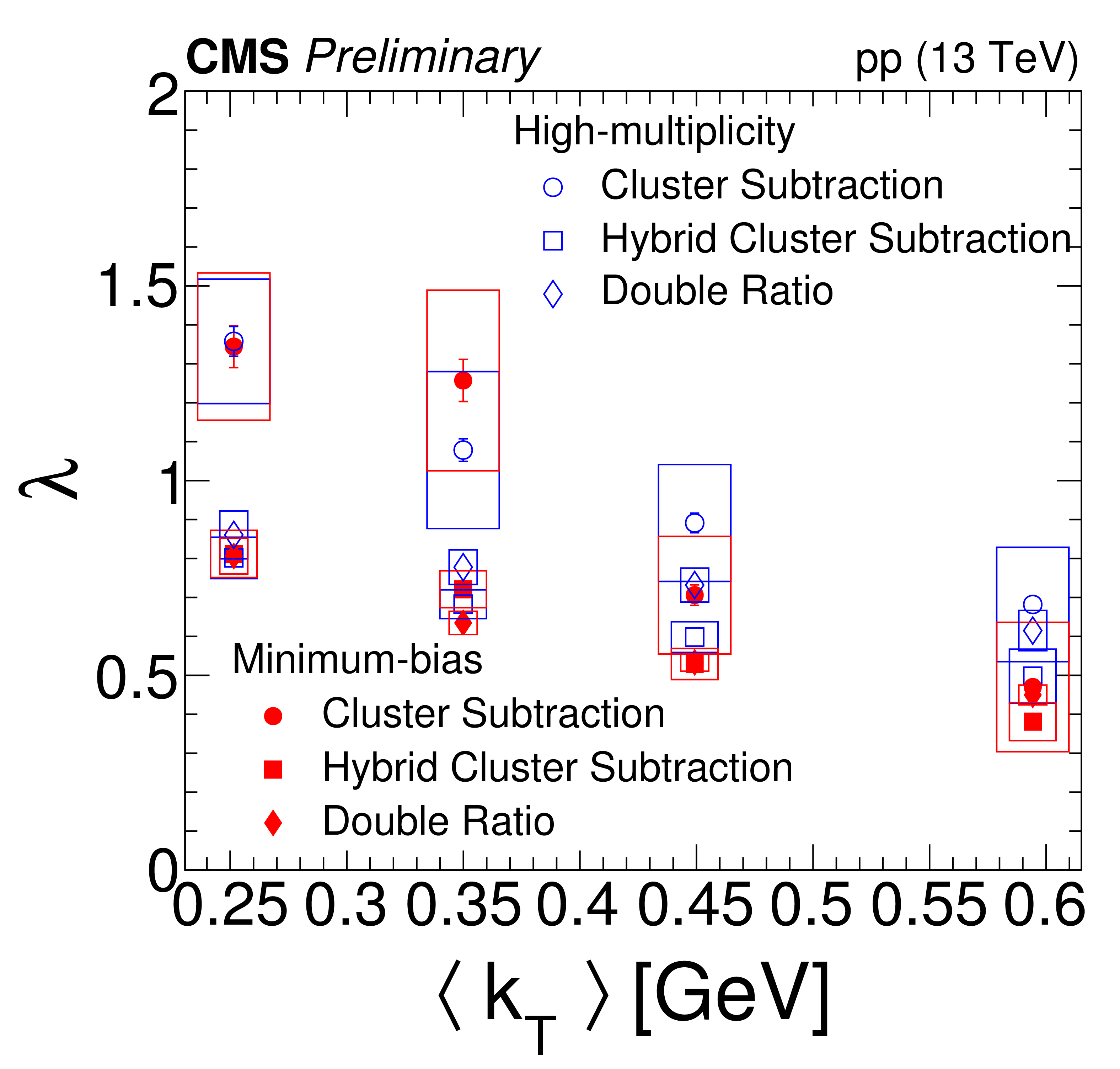
Figure 4:
Results for $ {R_\text {inv}} $ (left) and $\lambda $ (right) from the three methods as a function of multiplicity (top) and $ {k_{\mathrm {T}}} $ (bottom). In the top plots, statistical and systematical uncertainties are represented by internal and external error bars, respectively. In the bottom plots, statistical and systematic uncertainties are shown as error bars and open boxes, respectively. |
png pdf |
Figure 4-a:
Results for $ {R_\text {inv}} $ (left) and $\lambda $ (right) from the three methods as a function of multiplicity (top) and $ {k_{\mathrm {T}}} $ (bottom). In the top plots, statistical and systematical uncertainties are represented by internal and external error bars, respectively. In the bottom plots, statistical and systematic uncertainties are shown as error bars and open boxes, respectively. |

png pdf |
Figure 4-b:
Results for $ {R_\text {inv}} $ (left) and $\lambda $ (right) from the three methods as a function of multiplicity (top) and $ {k_{\mathrm {T}}} $ (bottom). In the top plots, statistical and systematical uncertainties are represented by internal and external error bars, respectively. In the bottom plots, statistical and systematic uncertainties are shown as error bars and open boxes, respectively. |
png pdf |
Figure 4-c:
Results for $ {R_\text {inv}} $ (left) and $\lambda $ (right) from the three methods as a function of multiplicity (top) and $ {k_{\mathrm {T}}} $ (bottom). In the top plots, statistical and systematical uncertainties are represented by internal and external error bars, respectively. In the bottom plots, statistical and systematic uncertainties are shown as error bars and open boxes, respectively. |
png pdf |
Figure 4-d:
Results for $ {R_\text {inv}} $ (left) and $\lambda $ (right) from the three methods as a function of multiplicity (top) and $ {k_{\mathrm {T}}} $ (bottom). In the top plots, statistical and systematical uncertainties are represented by internal and external error bars, respectively. In the bottom plots, statistical and systematic uncertainties are shown as error bars and open boxes, respectively. |

png pdf |
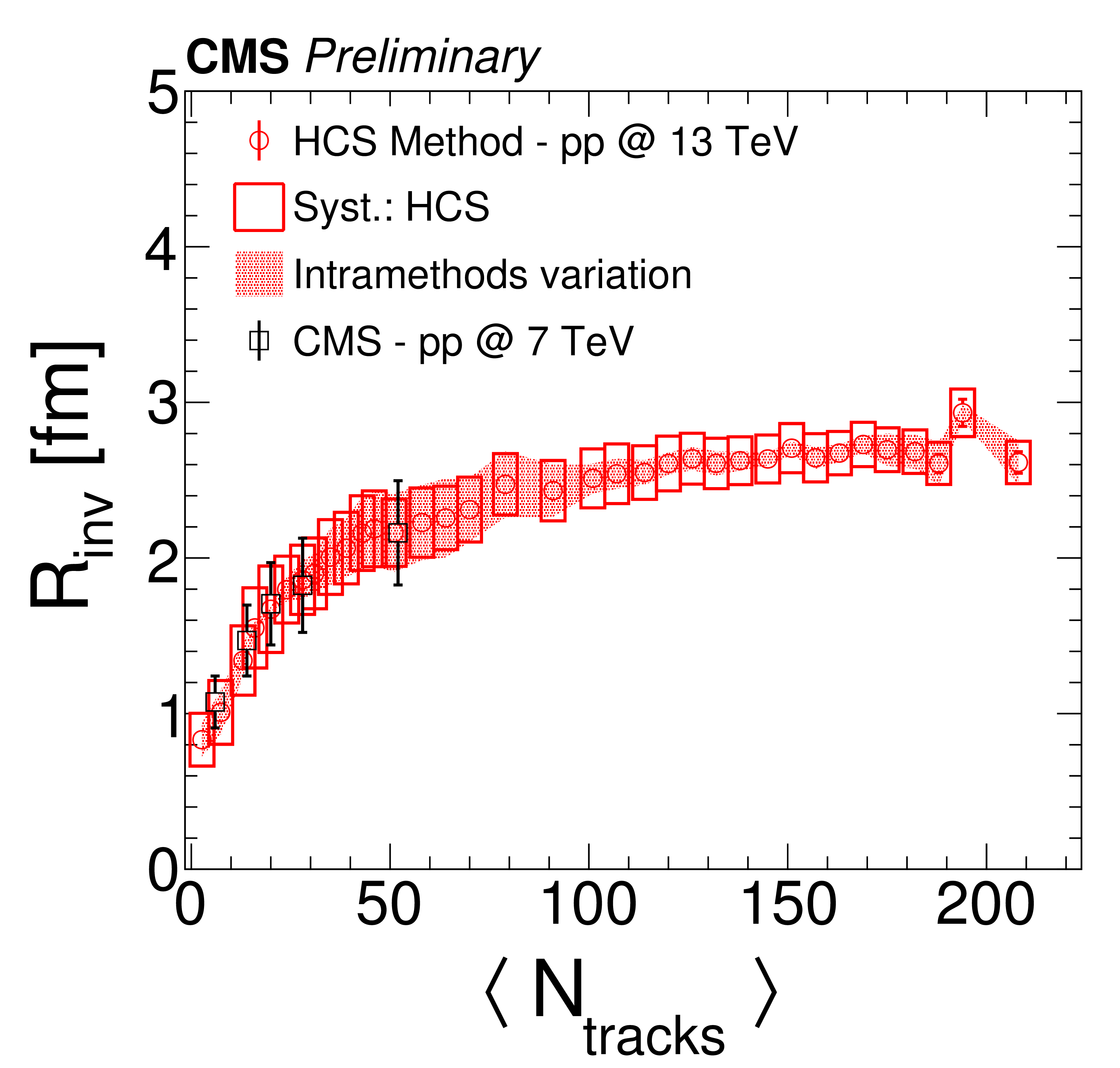
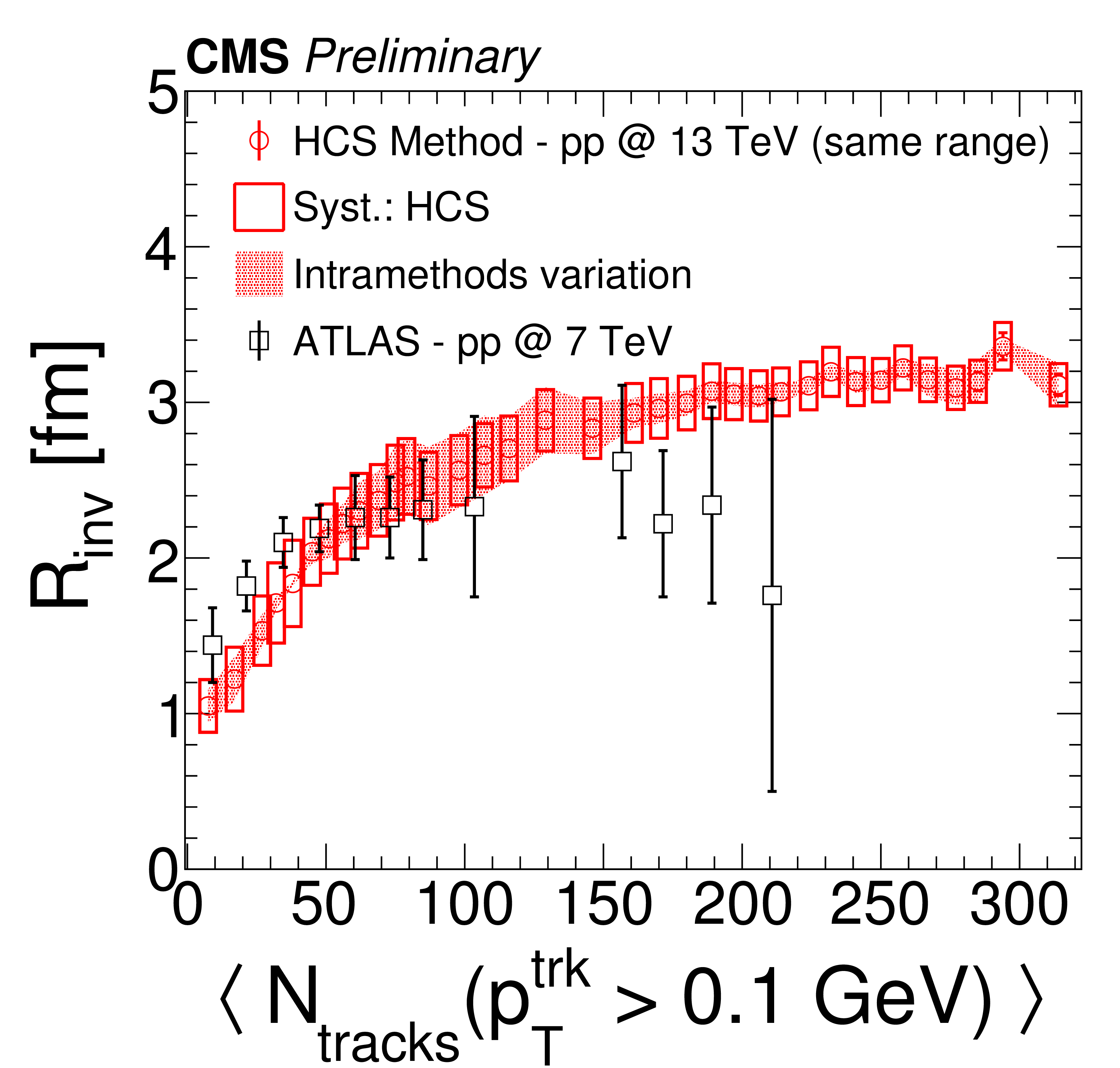
Figure 5:
Radius fit parameters as a function of particle level multiplicities using the HCS method in pp collisions at 13 TeV compared to results for pp collisions at 7 TeV from CMS (left) and ATLAS (right). Both the ordinate and abscissa for the CMS data in the right plot have been adjusted for compatibility with the ATLAS analysis procedure. See text for details. The error bars in the CMS [4] case represent systematic uncertainties (statistical ones are smaller than the marker size) and in the ATLAS [14] case, statistical and systematic uncertainties added in quadrature. |
png pdf |
Figure 5-a:
Radius fit parameters as a function of particle level multiplicities using the HCS method in pp collisions at 13 TeV compared to results for pp collisions at 7 TeV from CMS (left) and ATLAS (right). Both the ordinate and abscissa for the CMS data in the right plot have been adjusted for compatibility with the ATLAS analysis procedure. See text for details. The error bars in the CMS [4] case represent systematic uncertainties (statistical ones are smaller than the marker size) and in the ATLAS [14] case, statistical and systematic uncertainties added in quadrature. |
png pdf |
Figure 5-b:
Radius fit parameters as a function of particle level multiplicities using the HCS method in pp collisions at 13 TeV compared to results for pp collisions at 7 TeV from CMS (left) and ATLAS (right). Both the ordinate and abscissa for the CMS data in the right plot have been adjusted for compatibility with the ATLAS analysis procedure. See text for details. The error bars in the CMS [4] case represent systematic uncertainties (statistical ones are smaller than the marker size) and in the ATLAS [14] case, statistical and systematic uncertainties added in quadrature. |
png pdf |
Figure 6:
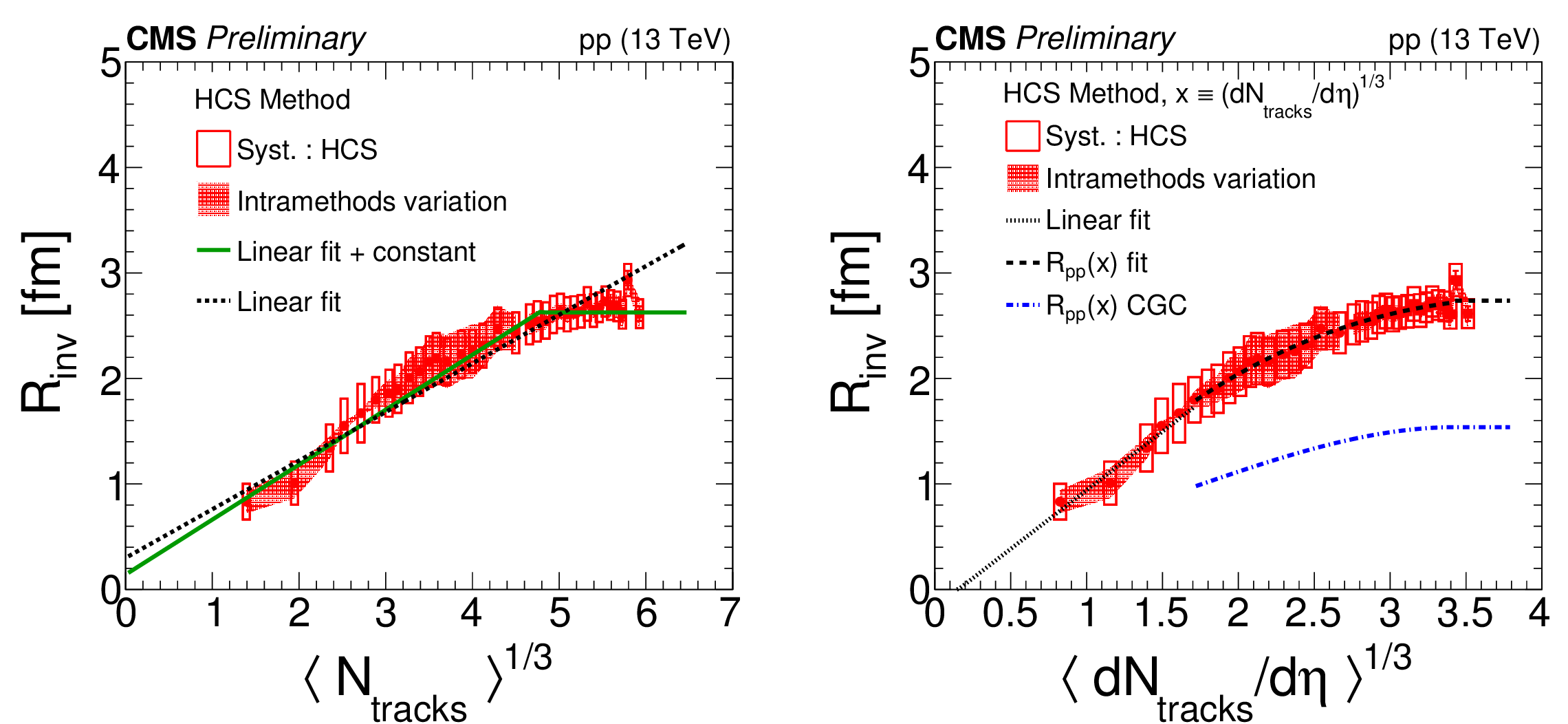
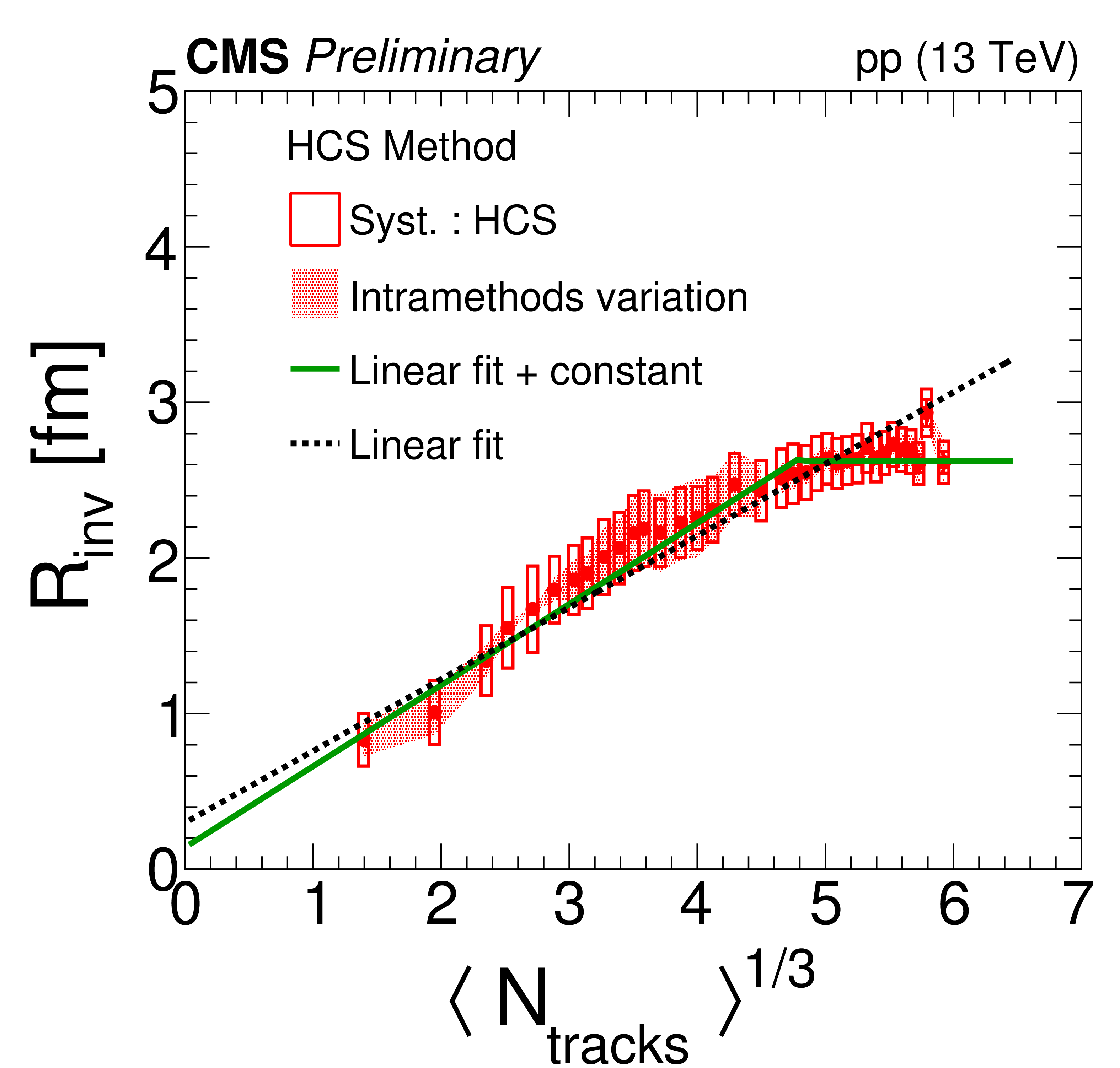
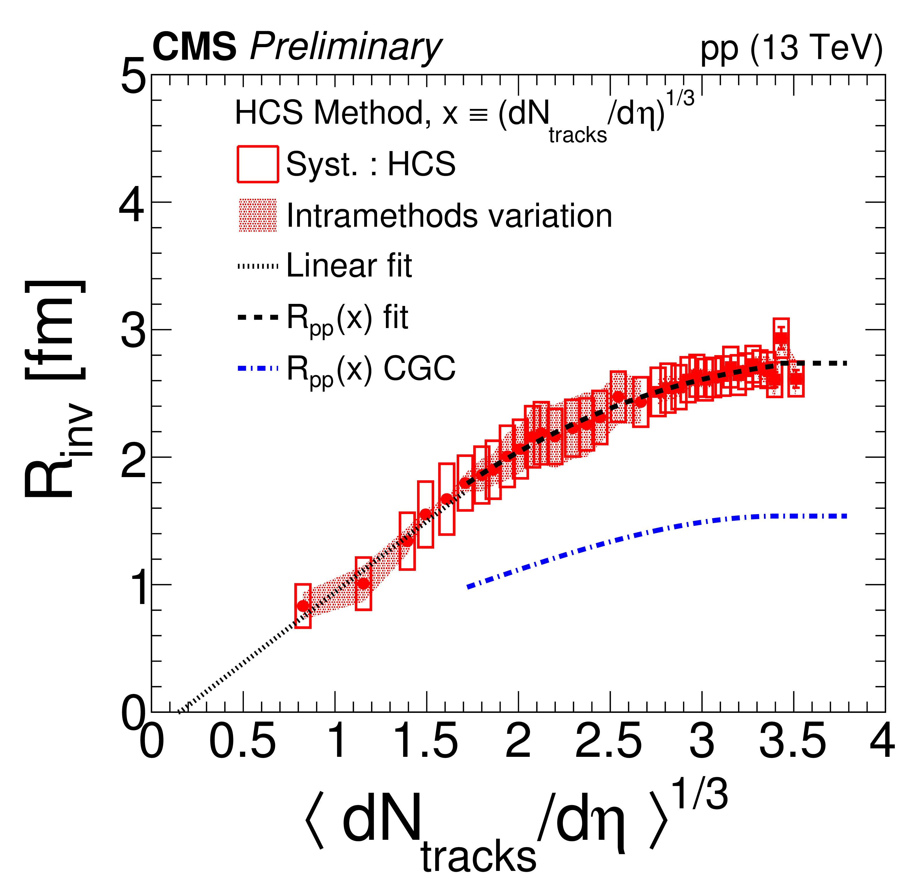
Comparison of $ {R_\text {inv}} $ obtained with the HCS method with theoretical expectations. Left: Values of $ {R_\text {inv}} $ as a function of $ < N_\text {tracks}> ^{1/3}$, with two fit functions: a single linear function and a linear function plus a constant for $N_\text {tracks}^{1/3} > 4.8$. Right: Comparison of $ {R_\text {inv}} $ with the predictions from CGC, as a function of $(dN_\text {tracks}/d\eta)^{1/3}$. The fits for $(dN_\text {tracks}/d\eta)^{1/3} > 1.7$ are performed using Eq. (8), with parameter values in the second row of Table 2. A linear function is fitted for $(dN_\text {tracks}/d\eta)^{1/3} < 1.7$. Statistical uncertainties only are considered in all fits. |
png pdf |
Figure 6-a:
Comparison of $ {R_\text {inv}} $ obtained with the HCS method with theoretical expectations. Left: Values of $ {R_\text {inv}} $ as a function of $ < N_\text {tracks}> ^{1/3}$, with two fit functions: a single linear function and a linear function plus a constant for $N_\text {tracks}^{1/3} > 4.8$. Right: Comparison of $ {R_\text {inv}} $ with the predictions from CGC, as a function of $(dN_\text {tracks}/d\eta)^{1/3}$. The fits for $(dN_\text {tracks}/d\eta)^{1/3} > 1.7$ are performed using Eq. (8), with parameter values in the second row of Table 2. A linear function is fitted for $(dN_\text {tracks}/d\eta)^{1/3} < 1.7$. Statistical uncertainties only are considered in all fits. |
png pdf |
Figure 6-b:
Comparison of $ {R_\text {inv}} $ obtained with the HCS method with theoretical expectations. Left: Values of $ {R_\text {inv}} $ as a function of $ < N_\text {tracks}> ^{1/3}$, with two fit functions: a single linear function and a linear function plus a constant for $N_\text {tracks}^{1/3} > 4.8$. Right: Comparison of $ {R_\text {inv}} $ with the predictions from CGC, as a function of $(dN_\text {tracks}/d\eta)^{1/3}$. The fits for $(dN_\text {tracks}/d\eta)^{1/3} > 1.7$ are performed using Eq. (8), with parameter values in the second row of Table 2. A linear function is fitted for $(dN_\text {tracks}/d\eta)^{1/3} < 1.7$. Statistical uncertainties only are considered in all fits. |
png pdf |
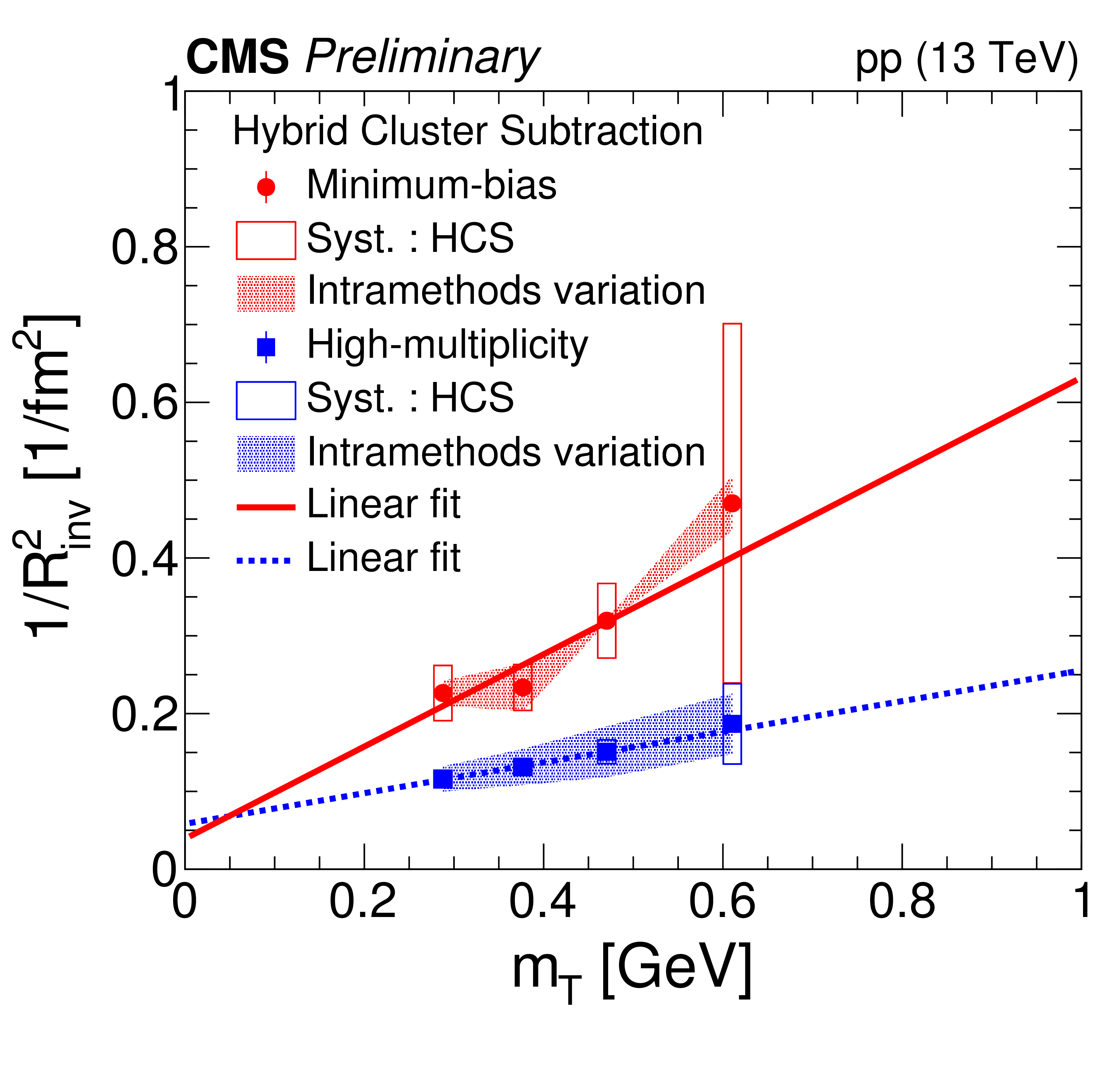
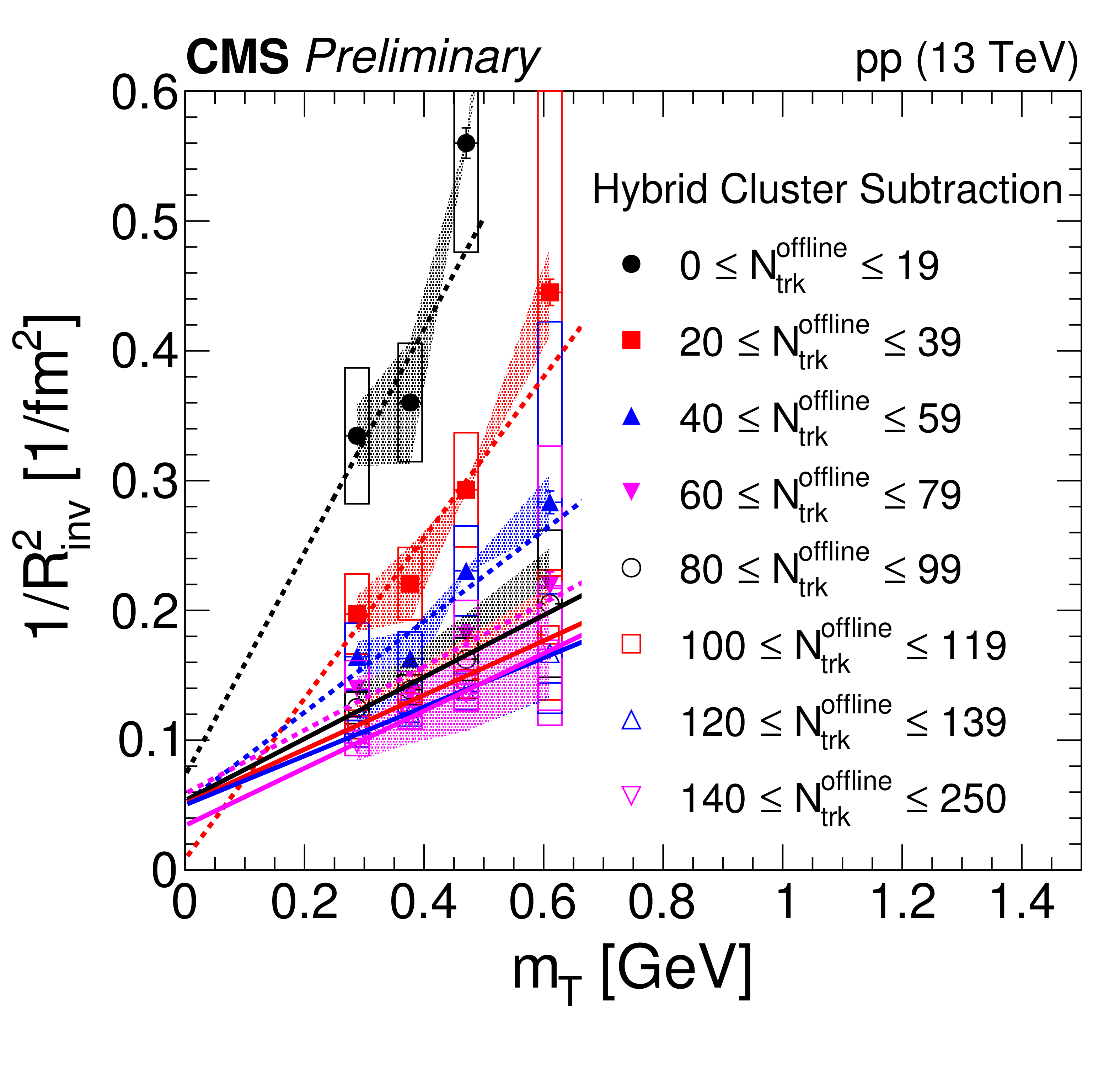
Figure 7:
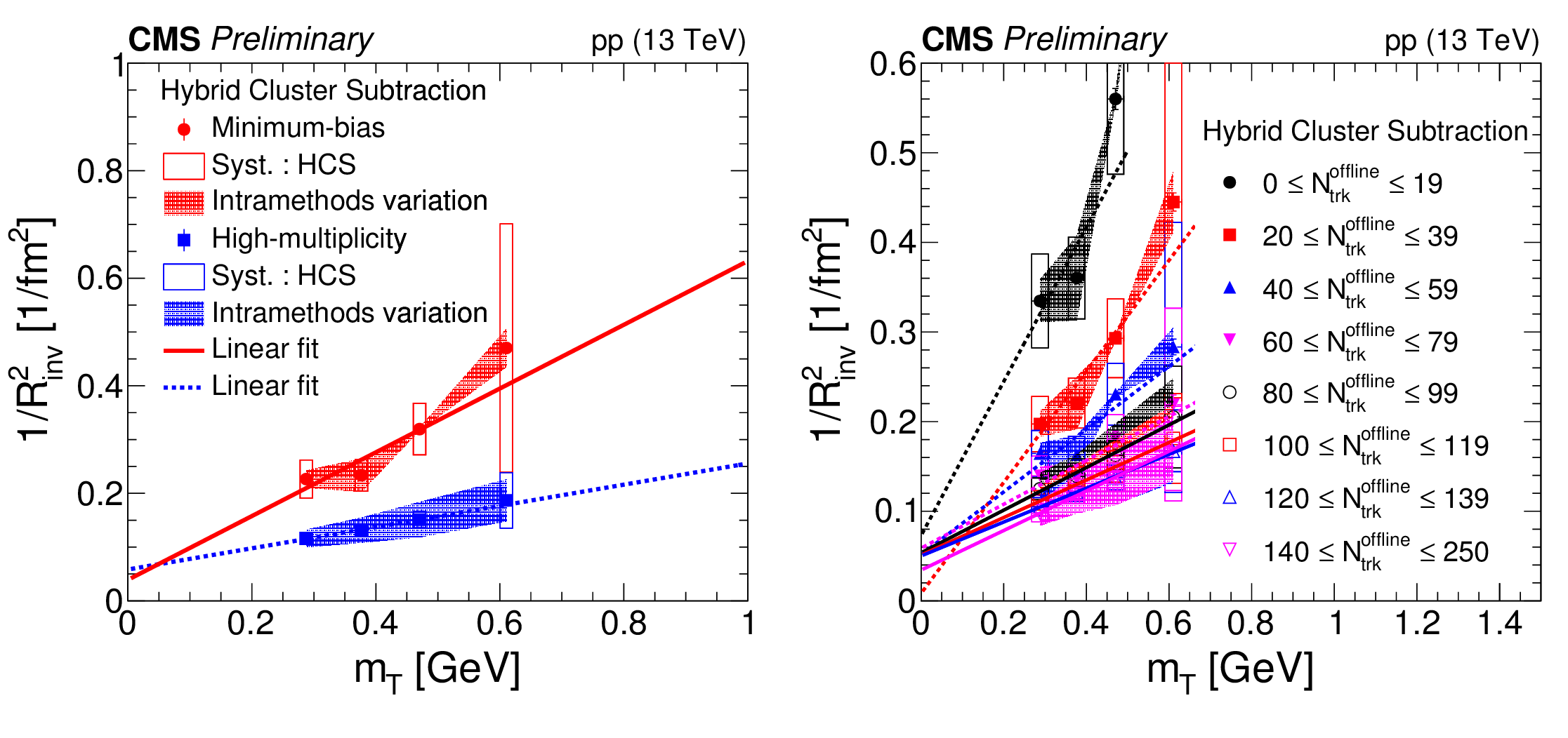
$1/R_{\mathrm {inv}}^2$ as a function of $m_{\mathrm {T}} = \sqrt {m_{\pi}^2 + < {k_{\mathrm {T}}} > ^2}$ for the HCS method. The MB range corresponds to 0 $ \le N_\text {trk}^\text {offline} \le $ 79 and the HM one, to 80 $ \le N_\text {trk}^\text {offline} \le $ 250. Statistical uncertainties are represented by error bars, systematic uncertainties related to the HCS method are shown as open boxes and the relative uncertainties from the intramethods variation are represented by the shaded bands. Only statistical uncertainties are considered in all the fits. |
png pdf |
Figure 7-a:
$1/R_{\mathrm {inv}}^2$ as a function of $m_{\mathrm {T}} = \sqrt {m_{\pi}^2 + < {k_{\mathrm {T}}} > ^2}$ for the HCS method. The MB range corresponds to 0 $ \le N_\text {trk}^\text {offline} \le $ 79 and the HM one, to 80 $ \le N_\text {trk}^\text {offline} \le $ 250. Statistical uncertainties are represented by error bars, systematic uncertainties related to the HCS method are shown as open boxes and the relative uncertainties from the intramethods variation are represented by the shaded bands. Only statistical uncertainties are considered in all the fits. |
png pdf |
Figure 7-b:
$1/R_{\mathrm {inv}}^2$ as a function of $m_{\mathrm {T}} = \sqrt {m_{\pi}^2 + < {k_{\mathrm {T}}} > ^2}$ for the HCS method. The MB range corresponds to 0 $ \le N_\text {trk}^\text {offline} \le $ 79 and the HM one, to 80 $ \le N_\text {trk}^\text {offline} \le $ 250. Statistical uncertainties are represented by error bars, systematic uncertainties related to the HCS method are shown as open boxes and the relative uncertainties from the intramethods variation are represented by the shaded bands. Only statistical uncertainties are considered in all the fits. |
png pdf |
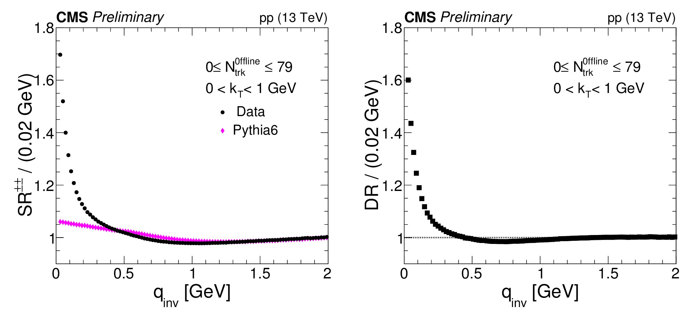
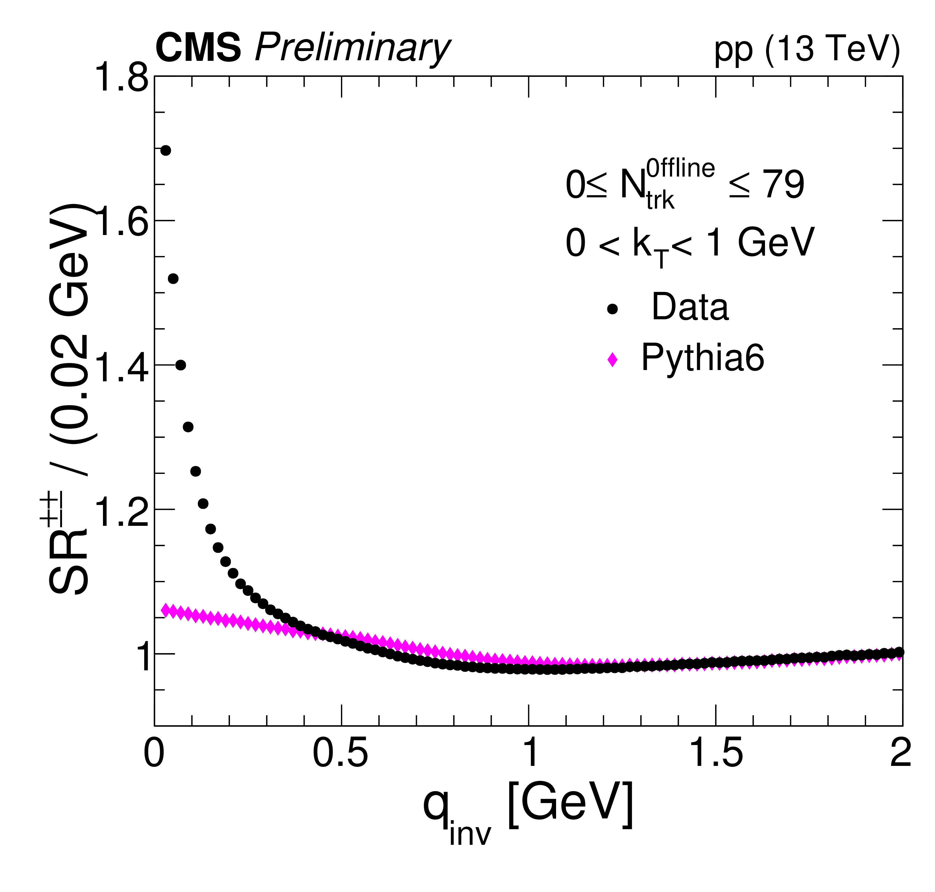
Figure 8:
Illustration of the steps in the DR method. Left: The SR in data is constructed, followed by a similar procedure with MC (PYTHIA6 $\mathrm {Z2}^{*}$) generated events. Right: The ratio of the two curves on the left taken to define the DR. The reference sample is obtained with the $\eta $-mixing procedure. All results correspond to integrated values in $N^\text {offline}_\text {trk}$ and $k_T$. |
png pdf |
Figure 8-a:
Illustration of the steps in the DR method. Left: The SR in data is constructed, followed by a similar procedure with MC (PYTHIA6 $\mathrm {Z2}^{*}$) generated events. Right: The ratio of the two curves on the left taken to define the DR. The reference sample is obtained with the $\eta $-mixing procedure. All results correspond to integrated values in $N^\text {offline}_\text {trk}$ and $k_T$. |
png pdf |
Figure 8-b:
Illustration of the steps in the DR method. Left: The SR in data is constructed, followed by a similar procedure with MC (PYTHIA6 $\mathrm {Z2}^{*}$) generated events. Right: The ratio of the two curves on the left taken to define the DR. The reference sample is obtained with the $\eta $-mixing procedure. All results correspond to integrated values in $N^\text {offline}_\text {trk}$ and $k_T$. |
png pdf |
Figure 9:
Same-sign and opposite-sign SR correlation functions are shown in different $N^\text {offline}_\text {track}$ and $ {k_{\mathrm {T}}} $ bins, together with the full fits (continuous curves) given in Eq. (10) and Eq. (13), for minimum-bias (top panel) and high-multiplicity (bottom panel) events. |
png pdf |
Figure 9-a:
Same-sign and opposite-sign SR correlation functions are shown in different $N^\text {offline}_\text {track}$ and $ {k_{\mathrm {T}}} $ bins, together with the full fits (continuous curves) given in Eq. (10) and Eq. (13), for minimum-bias (top panel) and high-multiplicity (bottom panel) events. |

png pdf |
Figure 9-b:
Same-sign and opposite-sign SR correlation functions are shown in different $N^\text {offline}_\text {track}$ and $ {k_{\mathrm {T}}} $ bins, together with the full fits (continuous curves) given in Eq. (10) and Eq. (13), for minimum-bias (top panel) and high-multiplicity (bottom panel) events. |
png pdf |
Figure 9-c:
Same-sign and opposite-sign SR correlation functions are shown in different $N^\text {offline}_\text {track}$ and $ {k_{\mathrm {T}}} $ bins, together with the full fits (continuous curves) given in Eq. (10) and Eq. (13), for minimum-bias (top panel) and high-multiplicity (bottom panel) events. |

png pdf |
Figure 9-d:
Same-sign and opposite-sign SR correlation functions are shown in different $N^\text {offline}_\text {track}$ and $ {k_{\mathrm {T}}} $ bins, together with the full fits (continuous curves) given in Eq. (10) and Eq. (13), for minimum-bias (top panel) and high-multiplicity (bottom panel) events. |
png pdf |
Figure 9-e:
Same-sign and opposite-sign SR correlation functions are shown in different $N^\text {offline}_\text {track}$ and $ {k_{\mathrm {T}}} $ bins, together with the full fits (continuous curves) given in Eq. (10) and Eq. (13), for minimum-bias (top panel) and high-multiplicity (bottom panel) events. |
png pdf |
Figure 9-f:
Same-sign and opposite-sign SR correlation functions are shown in different $N^\text {offline}_\text {track}$ and $ {k_{\mathrm {T}}} $ bins, together with the full fits (continuous curves) given in Eq. (10) and Eq. (13), for minimum-bias (top panel) and high-multiplicity (bottom panel) events. |
png pdf |
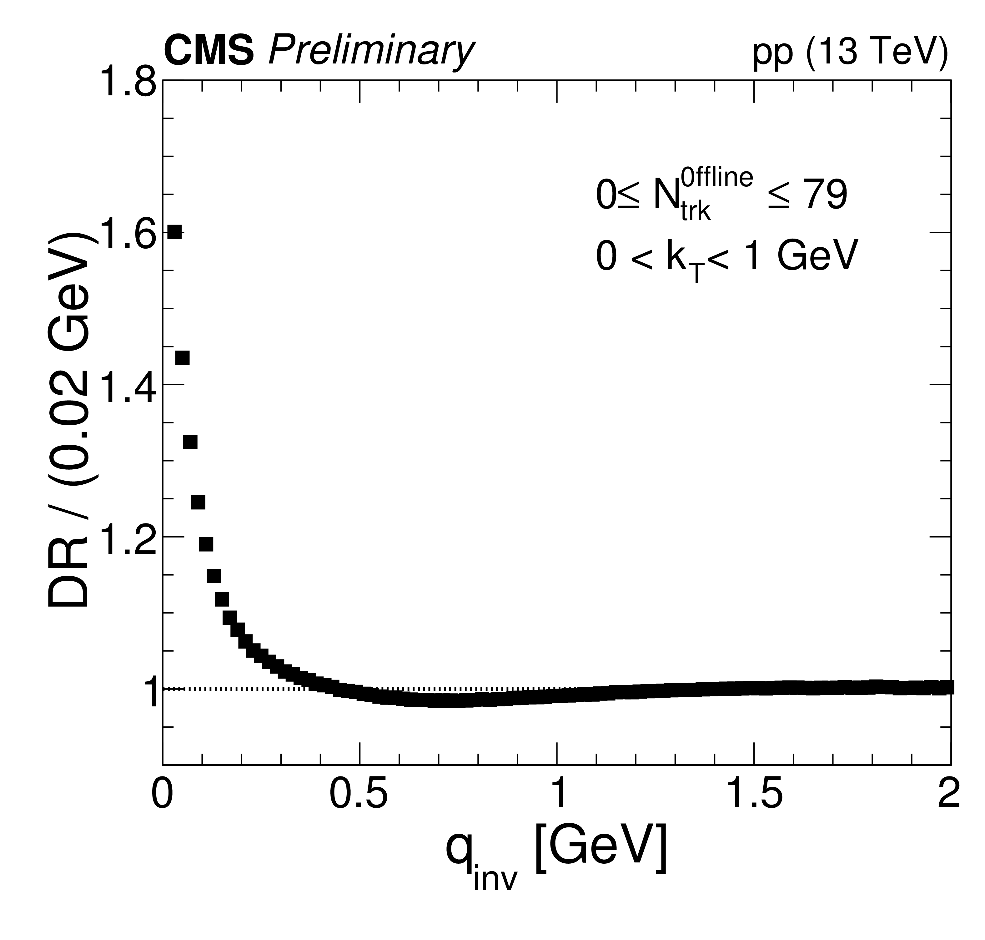
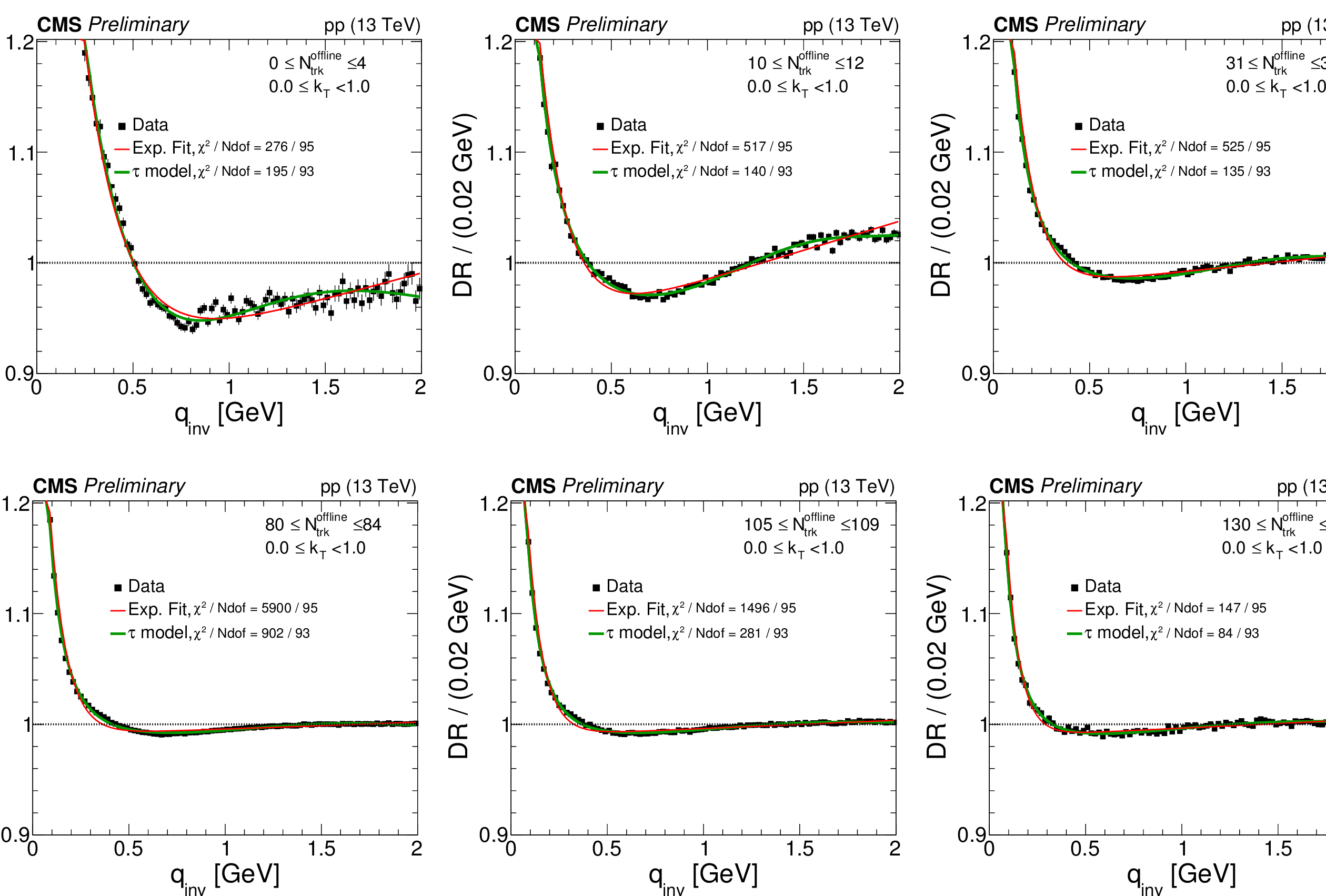
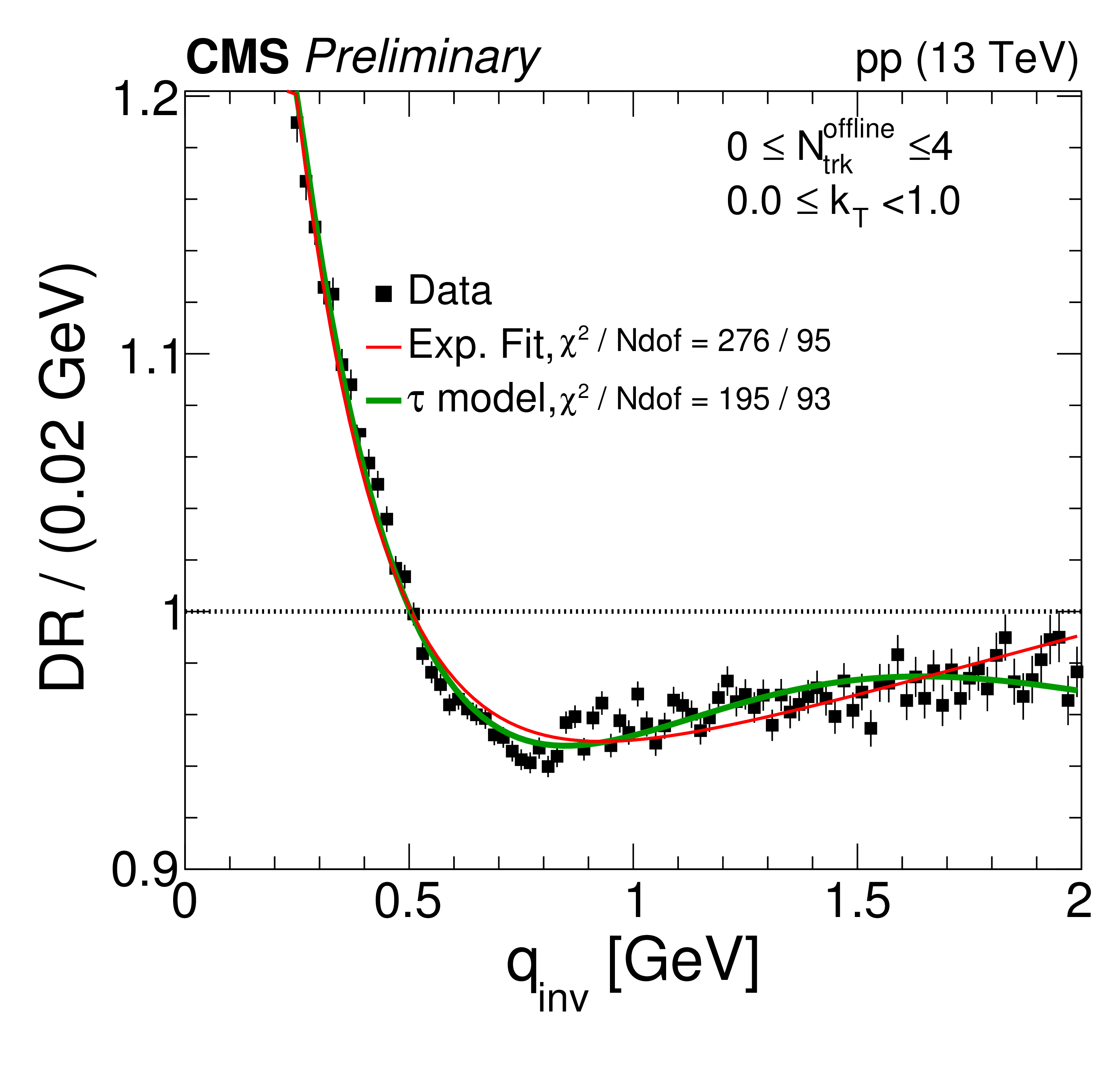
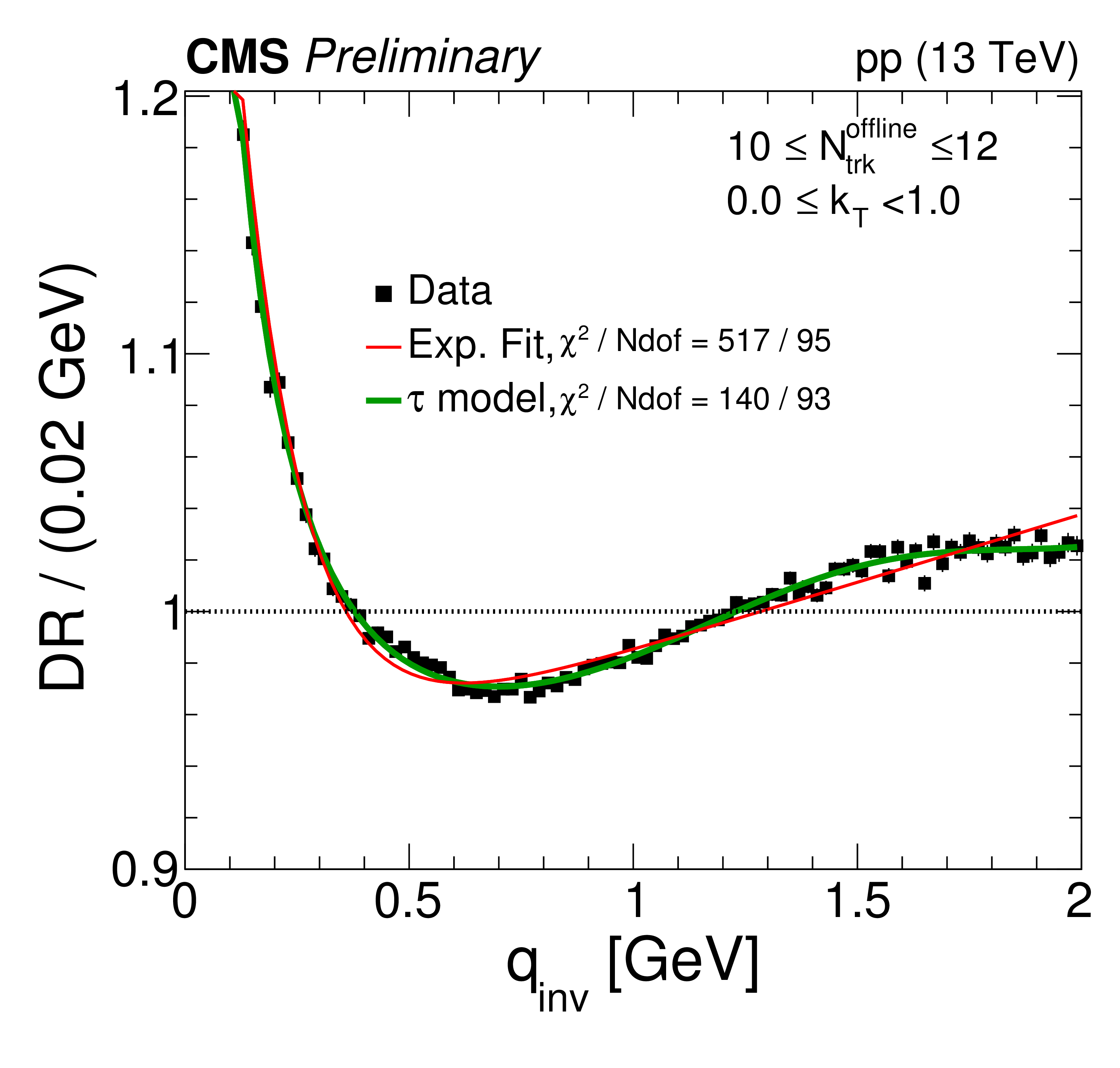
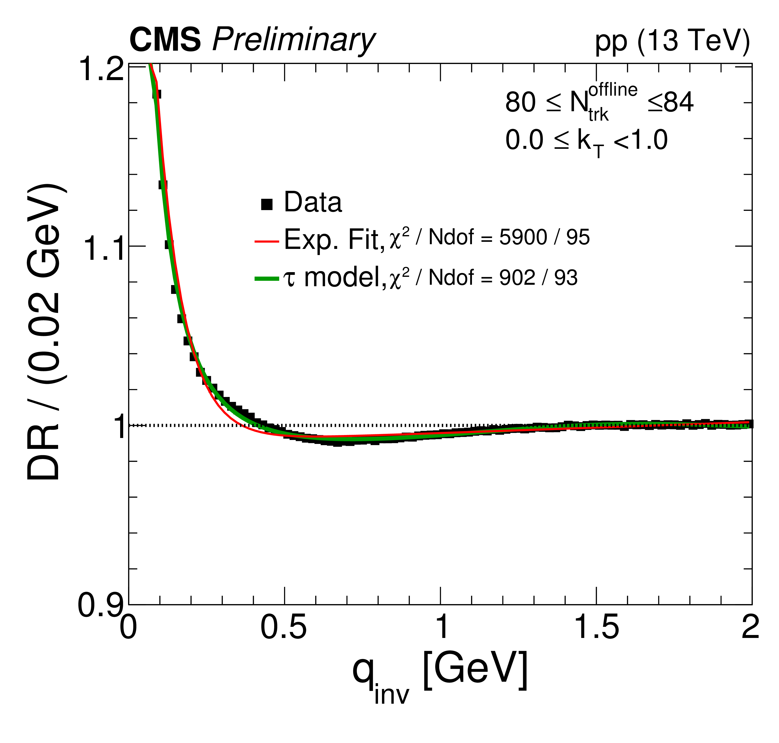
Figure 10:
Correlation functions from the DR technique, integrated in the range 0 $ < k_{\mathrm {T}} < $ 1 GeV, in six multiplicity bins. The results are zoomed along the vertical axis. |
png pdf |
Figure 10-a:
Correlation functions from the DR technique, integrated in the range 0 $ < k_{\mathrm {T}} < $ 1 GeV, in six multiplicity bins. The results are zoomed along the vertical axis. |
png pdf |
Figure 10-b:
Correlation functions from the DR technique, integrated in the range 0 $ < k_{\mathrm {T}} < $ 1 GeV, in six multiplicity bins. The results are zoomed along the vertical axis. |

png pdf |
Figure 10-c:
Correlation functions from the DR technique, integrated in the range 0 $ < k_{\mathrm {T}} < $ 1 GeV, in six multiplicity bins. The results are zoomed along the vertical axis. |
png pdf |
Figure 10-d:
Correlation functions from the DR technique, integrated in the range 0 $ < k_{\mathrm {T}} < $ 1 GeV, in six multiplicity bins. The results are zoomed along the vertical axis. |

png pdf |
Figure 10-e:
Correlation functions from the DR technique, integrated in the range 0 $ < k_{\mathrm {T}} < $ 1 GeV, in six multiplicity bins. The results are zoomed along the vertical axis. |

png pdf |
Figure 10-f:
Correlation functions from the DR technique, integrated in the range 0 $ < k_{\mathrm {T}} < $ 1 GeV, in six multiplicity bins. The results are zoomed along the vertical axis. |

png pdf |
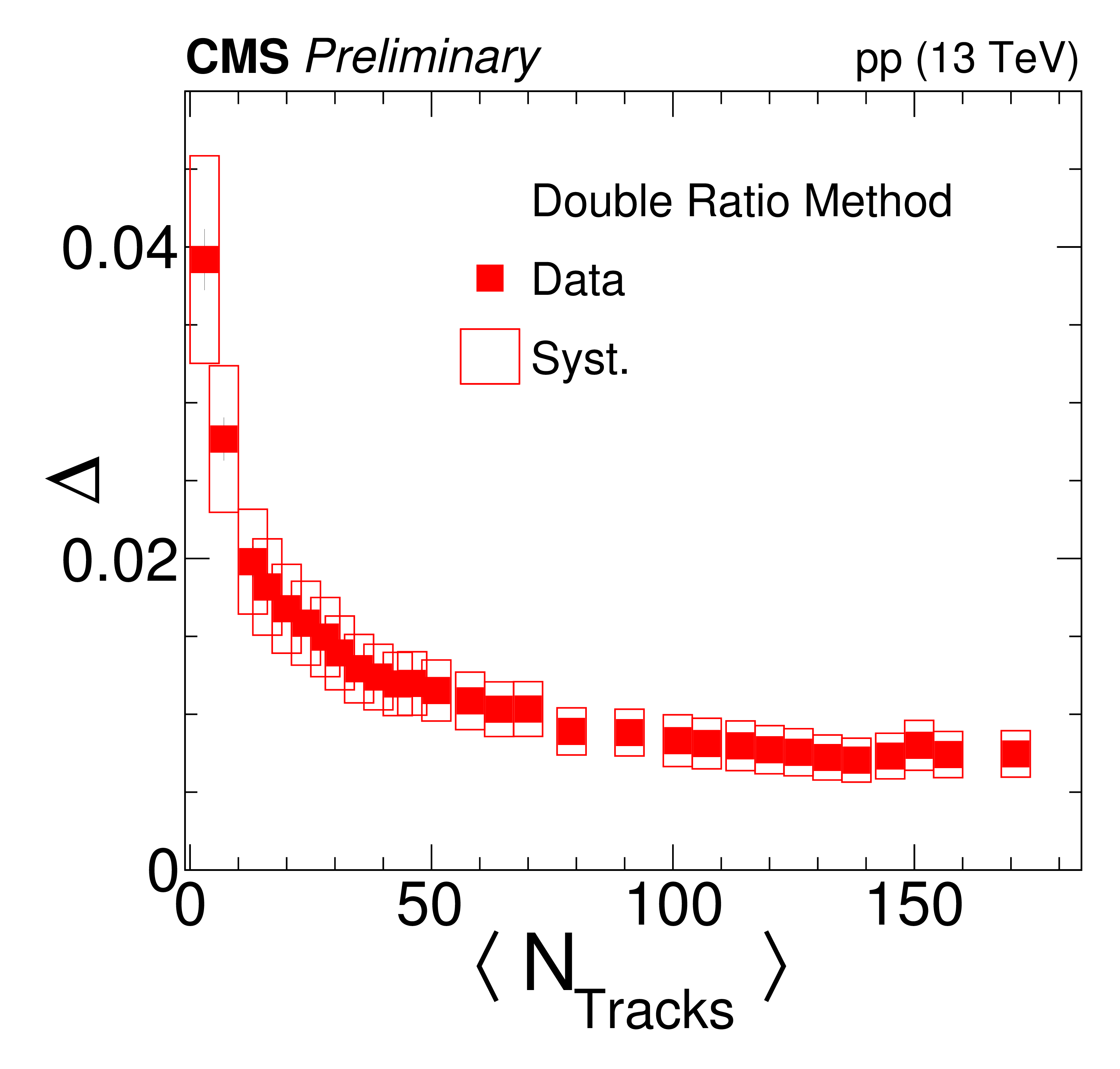
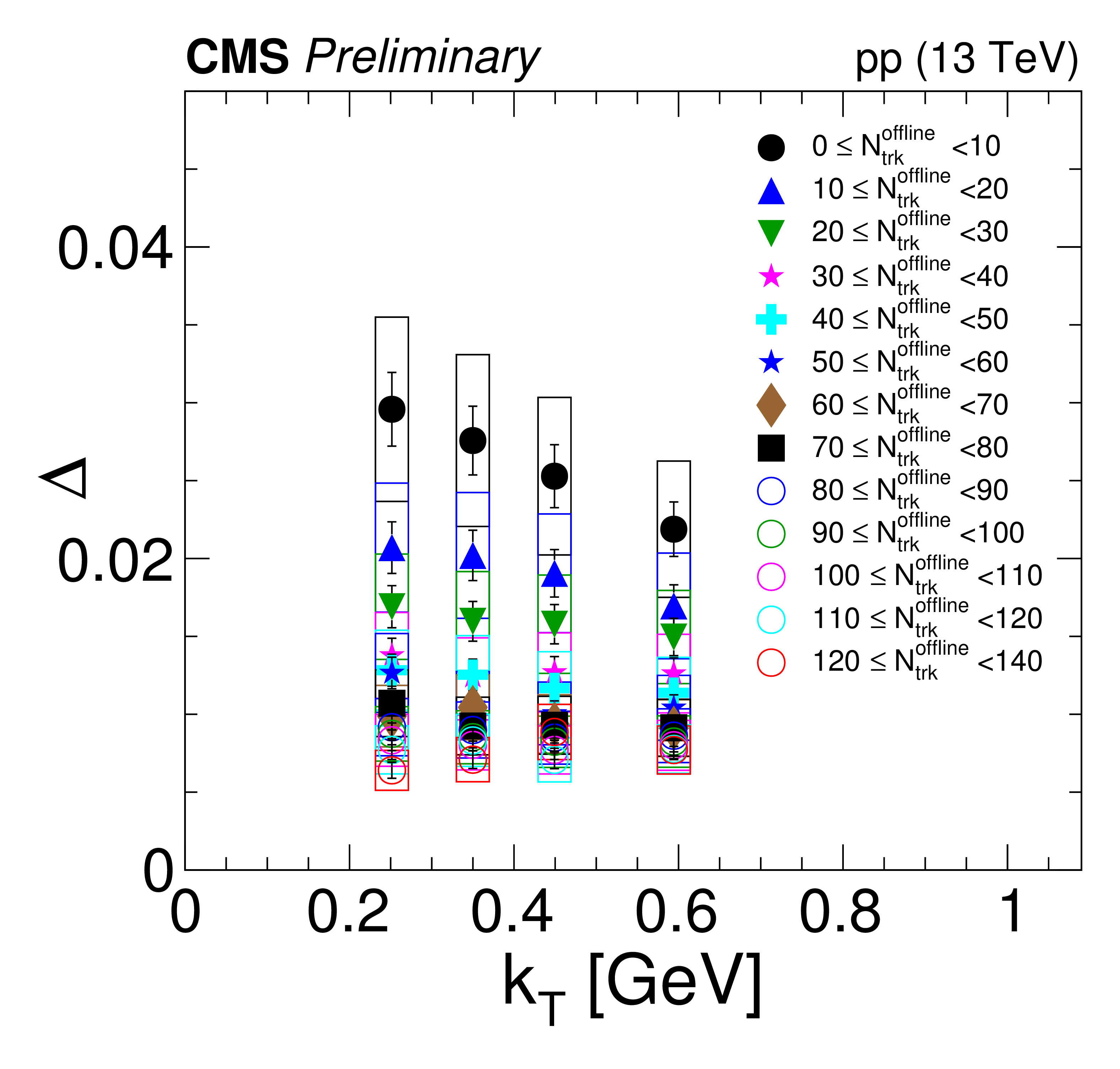
Figure 11:
Left: The depth of the anticorrelation $\Delta $ as a function of multiplicity (for $ {k_{\mathrm {T}}} $-integrated values) Right: $\Delta $ in finer bins of $N_\text {tracks}$ and $ {k_{\mathrm {T}}} $. The statistical uncertainties are represented by error bars, while the systematic ones are represented by open boxes. |
png pdf |
Figure 11-a:
Left: The depth of the anticorrelation $\Delta $ as a function of multiplicity (for $ {k_{\mathrm {T}}} $-integrated values) Right: $\Delta $ in finer bins of $N_\text {tracks}$ and $ {k_{\mathrm {T}}} $. The statistical uncertainties are represented by error bars, while the systematic ones are represented by open boxes. |
png pdf |
Figure 11-b:
Left: The depth of the anticorrelation $\Delta $ as a function of multiplicity (for $ {k_{\mathrm {T}}} $-integrated values) Right: $\Delta $ in finer bins of $N_\text {tracks}$ and $ {k_{\mathrm {T}}} $. The statistical uncertainties are represented by error bars, while the systematic ones are represented by open boxes. |
| Tables | |
png pdf |
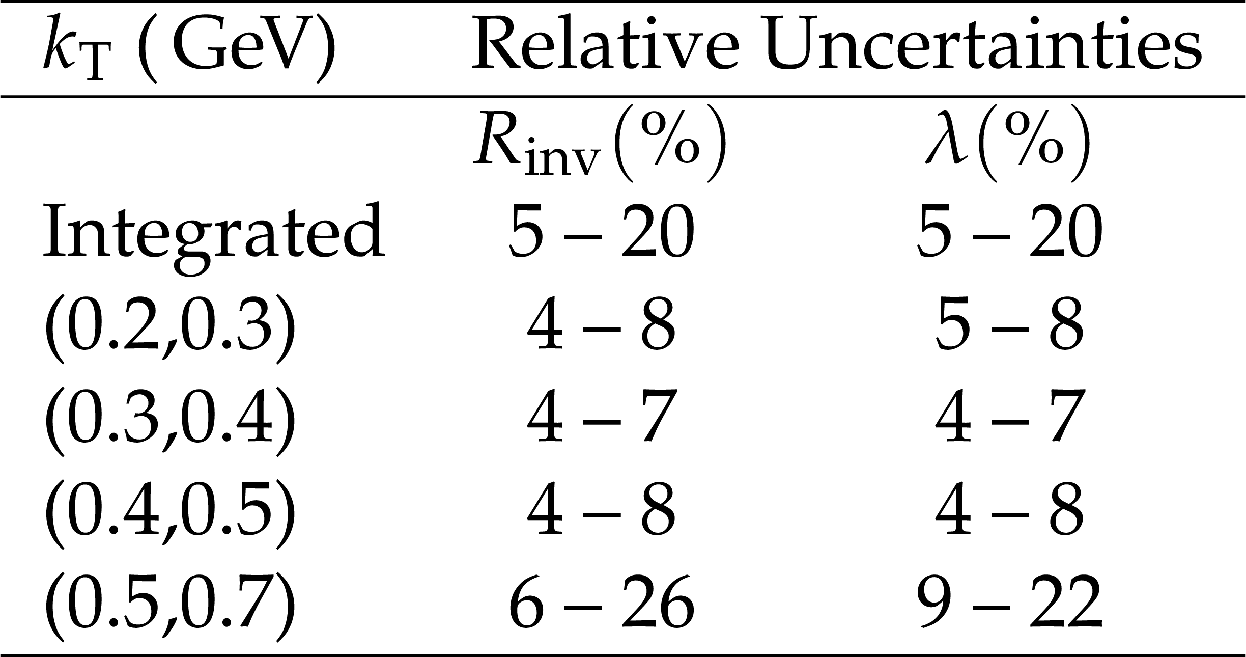
Table 1:
Total systematic uncertainties in different $ {k_{\mathrm {T}}} $ bins for the Hybrid Cluster Subtraction\ technique. The ranges in the uncertainties indicate the variation with $N^\text {offline}_\text {track}$. |

png pdf |
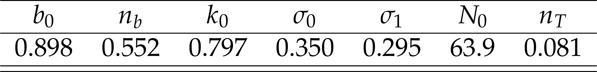
Table 2:
Parameter values refering to Eq. (8) from CGC calculations [59] in pp collsions at 7 TeV and from the fit to the data in Fig. 6 from pp collisions at 13 TeV. |
png pdf |
Table 3:
Values of the fit parameters from Eqs. (11) and (12), describing the cluster contribution in the data opposite-sign correlation function. |
| Summary |
|
A femtoscopic analysis of Bose-Einstein correlations has been performed using data from the CMS detector for proton-proton collisions at $\sqrt{s}= $ 13 TeV covering a broad range of charged particle multiplicity, from a few particles up to about 250 reconstructed charged hadrons. Three analysis methods, each with a different dependence on MC simulations, were used to generate correlation functions and were found to give consistent results. One dimensional studies of the lengths-of-homogeneity, $R_\text {inv}$, and the intercept parameter, $\lambda$, have been carried out for both inclusive events and high-multiplicity events selected using a dedicated online trigger. For multiplicities in the range 0 $ < N^\text {offline}_\text {track} < 250$ and average pair transverse momentum 0 $ < {k_{\mathrm{T}}} < 1$ GeV, values of the lengths of homogeneity and intercept are found to be in the range 0.8 $ < R_\text {inv} < $ 3.0 fm and 0.5 $ < \lambda < $ 1.0, respectively. Over most of the multiplicity range studied, the values of $R_\text {inv}$ increase with increasing event multiplicities and are observed to be proportional to $ < N_{\text{tracks}} > ^{1/3}$, a trend which is predicted by hydrodynamical calculations. For high-multiplicity events with more than $\approx$100 charged particles, the observed dependence of $R_\text {inv}$ suggests a possible saturation, with the lengths of homogeneity also consistent with a constant value. Comparisons of the multiplicity dependence are made with predictions of the CGC effective theory, by means of a parametrization of the radius of the system formed in pp collisions. The values of the radius parameters in the model are much lower than those in the data, although the general shape of the dependence on multiplicity is similar in both cases. The radius fit parameter $R_\text {inv}$ is also observed to decrease with increasing ${k_{\mathrm{T}}}$, a behavior that is consistent with emission from a system that is expanding prior to its decoupling. Inspired by hydrodynamic models, the dependence of $R_{\rm inv}^{-2}$ on the pair transverse mass was investigated and the two were observed to be proportional, a behavior similar to that seen in AA collisions. The proportionality constant between $R_{\rm inv}^{-2}$ and transverse mass can be related to the flow parameter of a Hubble type expansion of the system. For pp collisions at 13 TeV, this expansion was found to be slower for larger event multiplicity, a dependence which was also found in AA collisions. Therefore, the present analysis reveals additional similarities of the systems produced in high multiplicity pp collisions and those found using data for larger initial systems. These results may provide additional constrains for future attempts using hydrodynamical models and/or the CGC framework to explain the entire range of similarities between high multiplicity pp and heavy ion interactions. |
| References | ||||
| 1 | W. L. G. Goldhaber, S. Goldhaber and A. Pais | Influence of Bose-Einstein Statistics in the Antiproton-Proton Annihilation Process | PR120 (1960) 300 | |
| 2 | CMS Collaboration | First Measurement of Bose-Einstein Correlations in proton-proton Collisions at $ \sqrt{s} = $ 0.9 and 2.36 TeV at the LHC | PRL 105 (2010) 032001 | CMS-QCD-10-003 1005.3294 |
| 3 | CMS Collaboration | Measurement of Bose-Einstein Correlations in $ pp $ Collisions at $ \sqrt{s}= $ 0.9 and 7 TeV | JHEP 05 (2011) 029 | CMS-QCD-10-023 1101.3518 |
| 4 | CMS Collaboration | Bose-Einstein correlations in pp, pPb, and PbPb collisions at $ \sqrt{s} = $ 0.9 -- 7 TeV | To appear in PRC (2018) | CMS-FSQ-14-002 1712.07198 |
| 5 | AFS Collaboration | Bose-Esinstein correlations in $ \alpha \alpha $, $ pp $ and $ p\bar{p} $ interactions | PLB 129 (1983) 269 | |
| 6 | AFS Collaboration | Bose-Einstein correlations between kaons | PLB 155 (1985) 128 | |
| 7 | AFS Collaboration | Evidence of a directional dependence of Bose-Einstein correlations at the CERN Intersecting Storage Rings | PLB 187 (1987) 420 | |
| 8 | UA1 Collaboration | Bose-Einstein correlations in $ p \bar{p} $ interactions at $ \sqrt{s} = $ 0.2 to 0.9 TeV | PLB 226 (1989) 410 | |
| 9 | E735 Collaboration | Study of the source size in p pbar collisions at 1.8 TeV using pion interferometry | PRD 48 (1993) 1931 | |
| 10 | PHOBOS Collaboration | Transverse momentum and rapidity dependence of HBT correlations in Au + Au collisions at s(NN)**(1/2) = 62.4-GeV and 200-GeV | PRC 73 (2006) 031901 | nucl-ex/0409001 |
| 11 | STAR Collaboration | Pion interferometry in Au+Au collisions at S(NN)**(1/2) = 200-GeV | PRC 71 (2005) 044906 | nucl-ex/0411036 |
| 12 | PHENIX Collaboration | Source breakup dynamics in Au+Au Collisions at s(NN)**(1/2) = 200-GeV via three-dimensional two-pion source imaging | PRL 100 (2008) 232301 | 0712.4372 |
| 13 | ALICE Collaboration | Two-pion Bose-Einstein correlations in $ pp $ collisions at $ \sqrt{s}= $ 900 GeV | PRD 82 (2010) 052001 | 1007.0516 |
| 14 | ATLAS Collaboration | Two-Particle Bose-Einstein Correlations in pp collisions at $ \sqrt{s}= $ 0.9 and 7 TeV with the ATLAS detector | EPJC 75 (2015) 466 | 1502.07947 |
| 15 | LHCb Collaboration | Bose-Einstein correlations of same-sign charged pions in the forward region in $ pp $ collisions at $ \sqrt{s} = $ 7 TeV | JHEP 12 (2017) 025 | 1709.01769 |
| 16 | CMS Collaboration | Observation of Long-Range Near-Side Angular Correlations in Proton-Proton Collisions at the LHC | JHEP 1009 (2010) 091 | CMS-QCD-10-002 1009.4122 |
| 17 | CMS Collaboration | Observation of Long-Range Near-Side Angular Correlations in Proton-Proton Collisions at the LHC | JHEP 09 (2010) 091 | CMS-QCD-10-002 1009.4122 |
| 18 | ATLAS Collaboration | Observation of Long-Range Elliptic Azimuthal Anisotropies in $ \sqrt{s}= $ 13 and 2.76 TeV pp Collisions with the ATLAS Detector | PRL 116 (2016), no. 17, 172301 | 1509.04776 |
| 19 | CMS Collaboration | Observation of long-range near-side angular correlations in proton-lead collisions at the LHC | PLB 718 (2013) 795 | CMS-HIN-12-015 1210.5482 |
| 20 | ALICE Collaboration | Long-range angular correlations on the near and away side in p-Pb collisions at $ \sqrt{s_{NN}}= $ 5.02 TeV | PLB 719 (2013) 29 | 1212.2001 |
| 21 | ATLAS Collaboration | Observation of Associated Near-Side and Away-Side Long-Range Correlations in $ \sqrt{s_{NN}}= $ 5.02 TeV Proton-Lead Collisions with the ATLAS Detector | PRL 110 (2013), no. 18, 182302 | 1212.5198 |
| 22 | LHCb Collaboration | Measurements of long-range near-side angular correlations in $ \sqrt{s_{\text{NN}}}= $ 5 TeV proton-lead collisions in the forward region | PLB 762 (2016) 473 | 1512.00439 |
| 23 | CMS Collaboration | Evidence for collectivity in pp collisions at the LHC | PLB 765 (2017) 193 | CMS-HIN-16-010 1606.06198 |
| 24 | CMS Collaboration | Measurement of long-range near-side two-particle angular correlations in pp collisions at $ \sqrt s = $ 13 TeV | PRL 116 (2016), no. 17, 172302 | CMS-FSQ-15-002 1510.03068 |
| 25 | CMS Collaboration | The CMS experiment at the CERN LHC | JINST 3 (2008) S08004 | CMS-00-001 |
| 26 | T. Sjostrand, S. Mrenna, and P. Skands | PYTHIA 6.4 physics and manual | JHEP 05 (2006) 026 | hep-ph/0603175 |
| 27 | T. Sjostrand, S. Mrenna, and P. Z. Skands | A brief introduction to PYTHIA 8.1 | CPC 178 (2008) 852 | 0710.3820 |
| 28 | R. Field | Early LHC Underlying Event Data - Findings and Surprises | 1010.3558 | |
| 29 | CMS Collaboration | Event generator tunes obtained from underlying event and multiparton scattering measurements | EPJC 76 (2016), no. 3, 155 | CMS-GEN-14-001 1512.00815 |
| 30 | R. Corke and T. Sjostrand | Interleaved Parton Showers and Tuning Prospects | JHEP 03 (2011) 032 | 1011.1759 |
| 31 | T. Pierog et al. | EPOS LHC: Test of collective hadronization with data measured at the CERN Large Hadron Collider | PRC 92 (2015), no. 3, 034906 | 1306.0121 |
| 32 | S. Agostinelli et al. | Geant4---a simulation toolkit | NIMA 506 (2003) 250 | |
| 33 | CMS Collaboration | Description and performance of track and primary-vertex reconstruction with the CMS tracker | JINST 9 (2014), no. 10, P10009 | CMS-TRK-11-001 1405.6569 |
| 34 | CMS Collaboration | Measurement of transverse momentum relative to dijet systems in PbPb and pp collisions at $ \sqrt{s_{\mathrm{NN}}}= $ 2.76 TeV | JHEP 01 (2016) 006 | CMS-HIN-14-010 1509.09029 |
| 35 | CMS Collaboration | Study of the inclusive production of charged pions, kaons, and protons in pp collisions at $ \sqrt{s}= $ 0.9 , 2.76, and 7~TeV | EPJC 72 (2012) 2164 | CMS-FSQ-12-014 1207.4724 |
| 36 | Y. Sinyukov et al. | Coulomb corrections for interferometry analysis of expanding hadron systems | PLB 432 (1998) 248 | |
| 37 | M. Gyulassy, S. K. Kauffman, L. W. Wilson | Pion Interferometry o nuclear collisions. I. Theory | PRC 20 (1979) 2267 | |
| 38 | S. Pratt | Coherence and Coulomb effects on pion interferometry | PRD 33 (1986) 72 | |
| 39 | M. Biyajima and T. Mizoguchi | Coulomb wave function correction to Bose-Einstein correlations | SULDP-1994-9 | |
| 40 | M. Bowler | Coulomb corrections to Bose-Einstein correlations have been greatly exaggerated | PLB 270 (1991) 69 | |
| 41 | Y. Sinyukov et al. | Coulomb corrections for interferometry analysis of expanding hadron systems | PLB 432 (1998) 248 | |
| 42 | A. N. Makhlin and Y. M. Sinyukov | The hydrodynamics of hadron matter under a pion interferometric microscope | Z. Phys. C 39 (1988) 69 | |
| 43 | T. Csorgo, S. Hegyi, and W. A. Zajc | Bose-Einstein correlations for Levy stable source distributions | EPJC 36 (2004) 67 | nucl-th/0310042 |
| 44 | T. Csorgo, A. T. Szerzo, and S. Hegyi | Model independent shape analysis of correlations in one-dimension, two-dimensions or three-dimensions | PLB 489 (2000) 15 | hep-ph/9912220 |
| 45 | E802 Collaboration | System, centrality, and transverse mass dependence of two pion correlation radii in heavy ion collisions at 11.6 A-GeV and 14.6 A-GeV | PRC 66 (2002) 054906 | nucl-ex/0204001 |
| 46 | ATLAS Collaboration | Femtoscopy with identified charged pions in proton-lead collisions at $ \sqrt{s{NN}} = $ 5.02 TeV with ATLAS | PRC 96 (2017) 064908 | 1704.01621 |
| 47 | PHOBOS Collaboration | System size dependence of cluster properties from two-particle angular correlations in Cu+Cu and Au+Au collisions at $ \sqrt{s_{NN}} = $ 200~GeV | PRC 81 (2010) 024904 | 0812.1172 |
| 48 | Y. Hama and Sandra S. Padula | Bose-Einstein correlation of particles produced by expanding sources | PRD 37 (1988) 3237 | |
| 49 | J. C. Collins and M. J. Perry | Superdense matter: Neutrons or asymptotically free quarks? | PRL 34 (1975) 1353 | |
| 50 | N. Cabibbo and G. Parisi | Exponential hadronic spectrum and quark liberation | PLB 59 (1975) 67 | |
| 51 | B. A. Freedman and L. D. McLerran | Fermions and gauge vector mesons at finite temperature and density. 1. Formal techniques | PRD 16 (1977) 1130 | |
| 52 | E. V. Shuryak | Theory of hadronic plasma | Sov. Phys. JETP 47 (1978) 212.[Zh. Eksp. Teor. Fiz. 74, 408] | |
| 53 | M. I. Khalatnikov | Some questions onf the relativistic hydrodynamic | Zh. Eksp. Teor. Fiz. 26 (1954) 529 | |
| 54 | L. D. Landau | On the multiple production of particle sin high energy collisions | Izv. Adak. Nauk SSSR Ser. Fiz. 17 (1953) 51 | |
| 55 | R. Campanini and G. Ferri | Experimental equation of state in pp and $ p\bar{p} $ collisions and phase transition to quark gluon plasma | Phys. Letter. B 703 (2011) 237 | 1106.2008 |
| 56 | P. Bozek and W. Broniowski | Size of the emission source and collectivity in ultra-relativistic p-Pb collisions | PLB 720 (2013) 250 | 1301.3314 |
| 57 | V. M. Shapoval, P. Braun-Munzinger, I. A. Karpenko, and \relax Yu. M. Sinyukov | Femtoscopic scales in $ p+p $ and $ p+ $Pb collisions in view of the uncertainty principle | PLB 725 (2013) 139 | 1304.3815 |
| 58 | M. P. Larry McLerran and B. Schenke | Transverse momentum of protons, pions and kaons in high multiplicity pp and pA collisions: Evidence for the color glass condensate? | NP A 916 (2013) 210 | 1306.2350 |
| 59 | P. T. A. Bzdak, B. Schenke and R. Venugopalan | Initial-state geometry and the role of hydrodynamics in proton-proton, proton-nucleus, and deuteron-nucleus collisions | PRC 87 (2013) 064906 | 1304.3403 |
| 60 | T. Csorg\Ho and B. Lorstad | Bose-Einstein correlations for three-dimensionally expanding, cylindrically symmetric, finite systems | PRC 54 (1996) 1390 | hep-ph/9509213 |
| 61 | PHENIX Collaboration | Bose-Einstein correlations of charged pion pairs in Au + Au collisions at s(NN)**(1/2) = 200-GeV | PRL 93 (2004) 152302 | nucl-ex/0401003 |
| 62 | STAR Collaboration | Pion interferometry in Au+Au collisions at S(NN)**(1/2) = 200-GeV | PRC 71 (2005) 044906 | nucl-ex/0411036 |
| 63 | STAR Collaboration | Pion Interferometry in Au+Au and Cu+Cu Collisions at RHIC | PRC 80 (2009) 024905 | 0903.1296 |
| 64 | PHENIX Collaboration | Systematic study of charged-pion and kaon femtoscopy in Au + Au collisions at $ \sqrt{s_{_{NN}}} = $ 200 GeV | PRC 92 (2015), no. 3, 034914 | 1504.05168 |
| 65 | ZEUS Collaboration | Bose-Einstein correlations in one and two-dimensions in deep inelastic scattering | PLB 583 (2004) 231 | hep-ex/0311030 |
| 66 | L3 Collaboration | Test of the $ \tau $-Model of Bose-Einstein Correlations and Reconstruction of the Source Function in Hadronic Z-boson Decay at LEP | EPJC 71 (2011) 1648 | 1105.4788 |
| 67 | T. Csorg\Ho and J. Zim\'anyi | Pion Interferometry for Strongly Correlated Space-Time and Momentum Space | NP A 517 (1990) 588 | |
|
|
Compact Muon Solenoid LHC, CERN |
|

|

|

|

|

|