Processing math: 100%

Compact Muon Solenoid
LHC, CERN

Visit us: CMS Public Website, CMS Physics ; Contact us: CMS Publications Committee

CMS-PAS-BPH-23-005

Search for $CP$ violation in $\mathrm{D}^0\to\mathrm{K}^0_{\mathrm{S}}\mathrm{K}^0_{\mathrm{S}}$ decay from proton-proton collisions at 13 TeV

CMS Collaboration

26 March 2024

Abstract: A search is reported for $CP$ violation in the $\mathrm{D}^0\to\mathrm{K}^0_{\mathrm{S}}\mathrm{K}^0_{\mathrm{S}}$ decay, using data collected from proton-proton collisions at $\sqrt{s} =$ 13 TeV recorded by the CMS experiment in 2018. A dedicated data set of about 10 billion events containing a pair of b hadrons, nearly all of which decay to charm hadrons, is used. The flavor of the neutral D meson is determined by the pion charge in the reconstructed decays $\mathrm{D}^{*+}\to\mathrm{D}^0\pi^+$ and $\mathrm{D}^{*-}\to\overline{\mathrm{D}}^0\pi^-$. The $CP$ asymmetry in $\mathrm{D}^0\to\mathrm{K}^0_{\mathrm{S}}\mathrm{K}^0_{\mathrm{S}}$ is measured to be $A_{CP}(\mathrm{K}^0_{\mathrm{S}}\mathrm{K}^0_{\mathrm{S}}) =$ 6.2 $\pm$ 3.0 (stat) $\pm$ 0.2 (syst) $\pm$ 0.8 $(A_{CP}(\mathrm{K}^0_{\mathrm{S}}\pi^+\pi^-))$ %, where the last uncertainty is the $CP$ asymmetry in the $\mathrm{D}^0\to\mathrm{K}^0_{\mathrm{S}}\pi^+\pi^-$ decay. This result is consistent with no $CP$ violation within 2 standard deviations. This is the first measurement of $CP$ violation in the charm sector by the CMS experiment, and the first measurement of $CP$ asymmetry in the fully hadronic final state performed by CMS at the nominal LHC luminosity, using the new data parking technique.

Links: CDS record (PDF) ; CADI line (restricted) ; These preliminary results are superseded in this paper, Submitted to EPJC. The superseded preliminary plots can be found here.

Figures
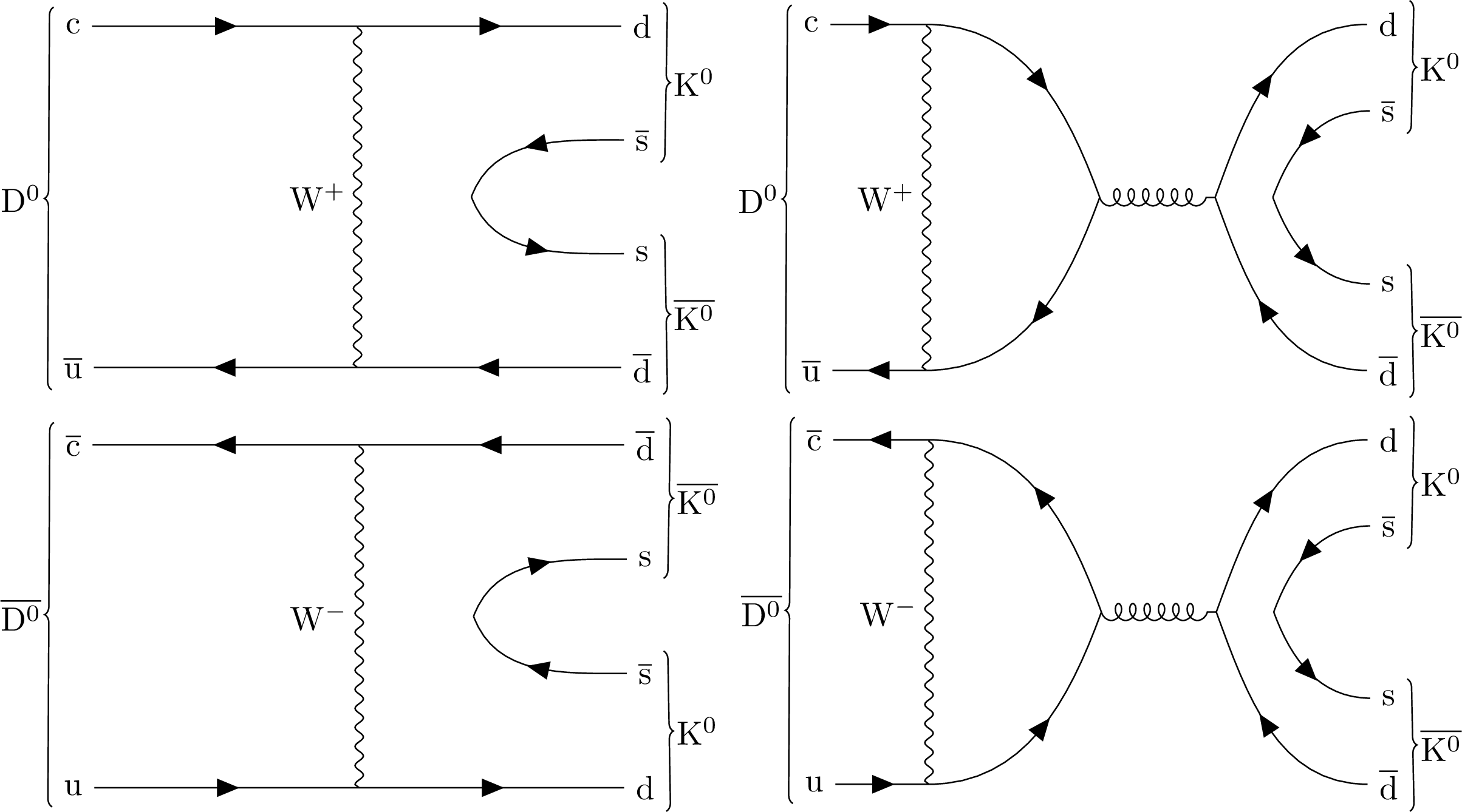
png pdf	Figure 1: The decay of neutral charm meson $\mathrm{D^0}$ (top) or $\overline{\mathrm{D}}^{0}$ (bottom) to two neutral kaons: exchange diagram (left) and penguin annihilation diagram (right).
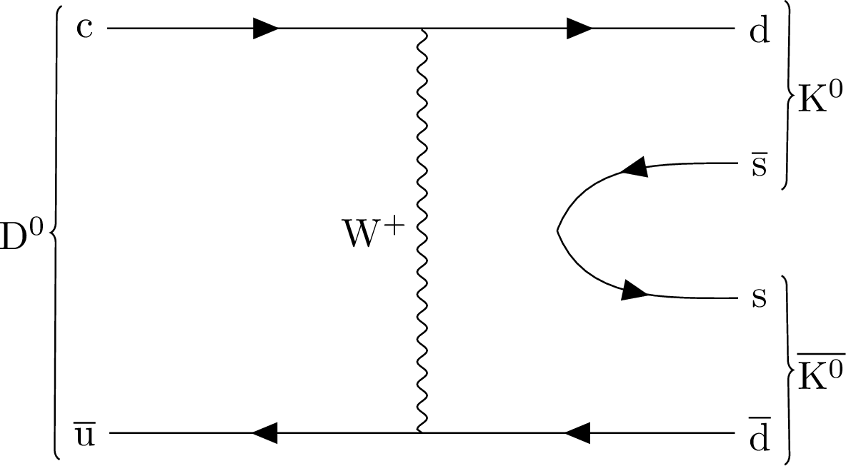
png pdf	Figure 1-a: The decay of neutral charm meson $\mathrm{D^0}$ (top) or $\overline{\mathrm{D}}^{0}$ (bottom) to two neutral kaons: exchange diagram (left) and penguin annihilation diagram (right).
png pdf	Figure 1-b: The decay of neutral charm meson $\mathrm{D^0}$ (top) or $\overline{\mathrm{D}}^{0}$ (bottom) to two neutral kaons: exchange diagram (left) and penguin annihilation diagram (right).
png pdf	Figure 1-c: The decay of neutral charm meson $\mathrm{D^0}$ (top) or $\overline{\mathrm{D}}^{0}$ (bottom) to two neutral kaons: exchange diagram (left) and penguin annihilation diagram (right).
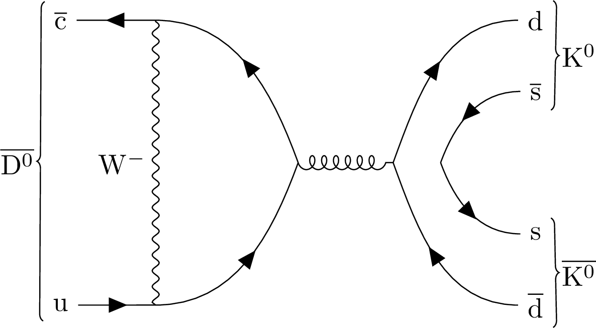
png pdf	Figure 1-d: The decay of neutral charm meson $\mathrm{D^0}$ (top) or $\overline{\mathrm{D}}^{0}$ (bottom) to two neutral kaons: exchange diagram (left) and penguin annihilation diagram (right).
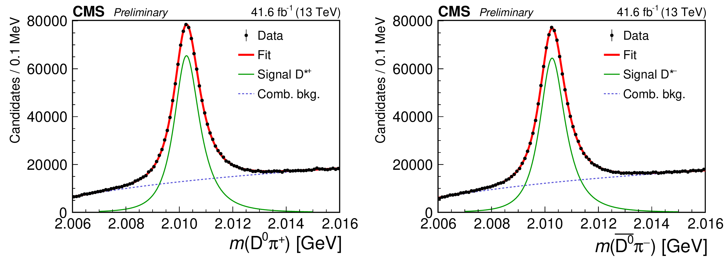
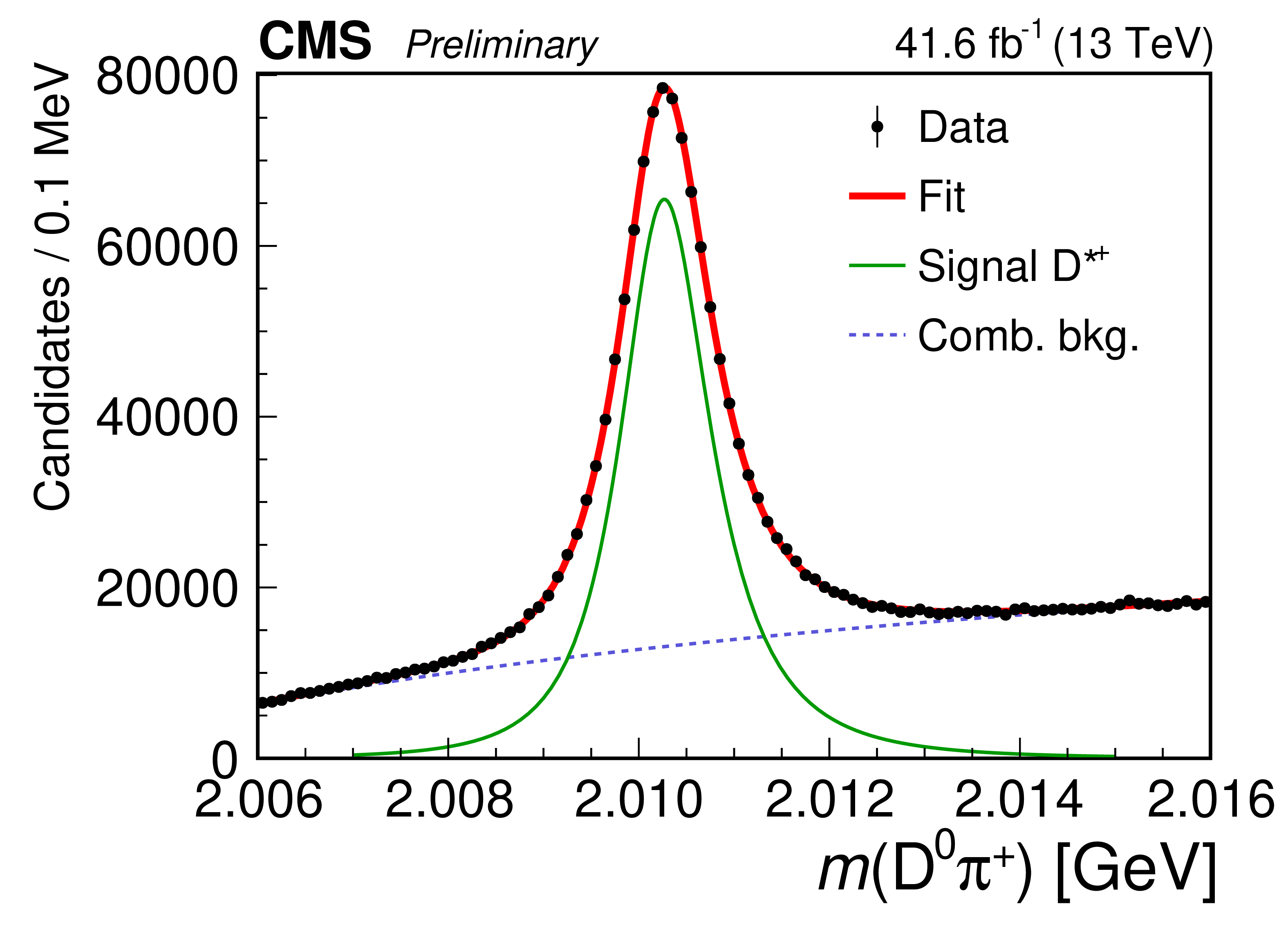
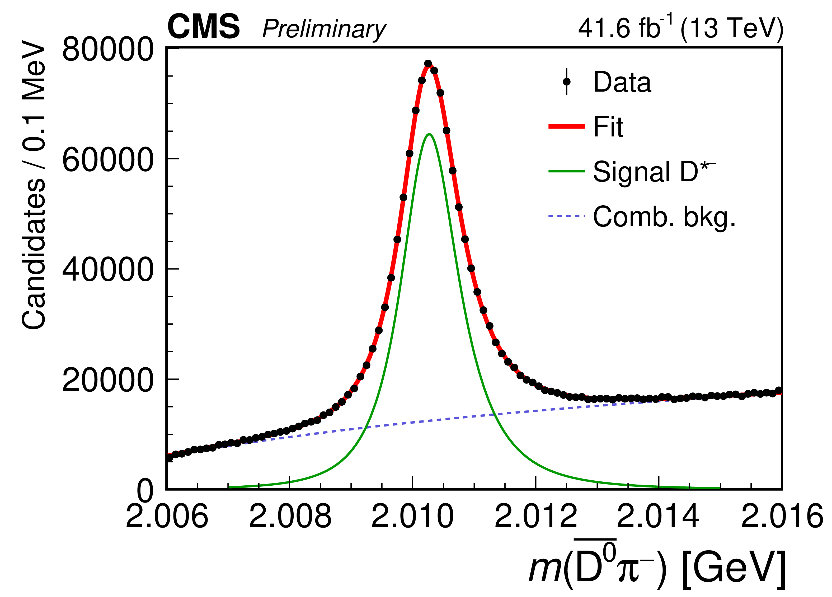
png pdf	Figure 2: Simultaneous fit of the $\mathrm{D}^{*+}$ (left) and $\mathrm{D}^{*-}$ (right) candidate invariant mass distributions in the $\mathrm{K^0_S}\pi^{+}\pi^{-}$ channel.
png pdf	Figure 2-a: Simultaneous fit of the $\mathrm{D}^{*+}$ (left) and $\mathrm{D}^{*-}$ (right) candidate invariant mass distributions in the $\mathrm{K^0_S}\pi^{+}\pi^{-}$ channel.
png pdf	Figure 2-b: Simultaneous fit of the $\mathrm{D}^{*+}$ (left) and $\mathrm{D}^{*-}$ (right) candidate invariant mass distributions in the $\mathrm{K^0_S}\pi^{+}\pi^{-}$ channel.
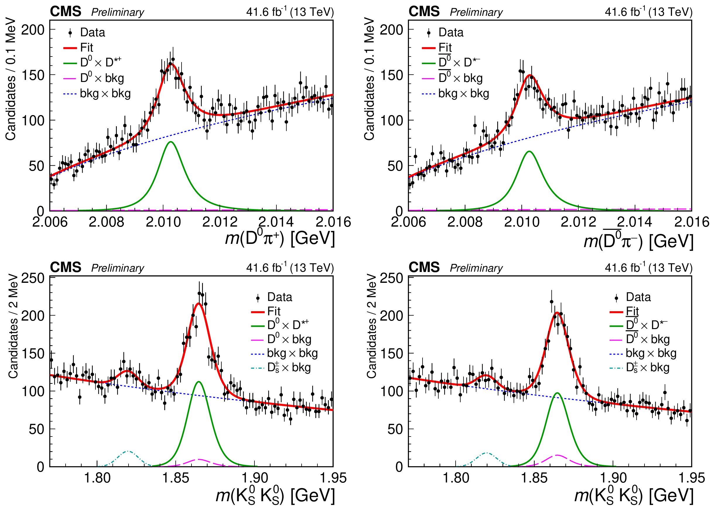
png pdf	Figure 3: Results of the 2D fit to $m(\mathrm{D}\pi^{\pm}) \times\ m(\mathrm{K^0_S}\mathrm{K^0_S})$ distribution for the signal channel, for $\mathrm{D}^{*+}$ (left) and $\mathrm{D}^{*-}$ (right) candidates: projections of the 2D fit on the $m(\mathrm{D}\pi^{\pm})$ (top) and $m(\mathrm{K^0_S}\mathrm{K^0_S})$ (bottom) axes.
png pdf	Figure 3-a: Results of the 2D fit to $m(\mathrm{D}\pi^{\pm}) \times\ m(\mathrm{K^0_S}\mathrm{K^0_S})$ distribution for the signal channel, for $\mathrm{D}^{*+}$ (left) and $\mathrm{D}^{*-}$ (right) candidates: projections of the 2D fit on the $m(\mathrm{D}\pi^{\pm})$ (top) and $m(\mathrm{K^0_S}\mathrm{K^0_S})$ (bottom) axes.
png pdf	Figure 3-b: Results of the 2D fit to $m(\mathrm{D}\pi^{\pm}) \times\ m(\mathrm{K^0_S}\mathrm{K^0_S})$ distribution for the signal channel, for $\mathrm{D}^{*+}$ (left) and $\mathrm{D}^{*-}$ (right) candidates: projections of the 2D fit on the $m(\mathrm{D}\pi^{\pm})$ (top) and $m(\mathrm{K^0_S}\mathrm{K^0_S})$ (bottom) axes.
png pdf	Figure 3-c: Results of the 2D fit to $m(\mathrm{D}\pi^{\pm}) \times\ m(\mathrm{K^0_S}\mathrm{K^0_S})$ distribution for the signal channel, for $\mathrm{D}^{*+}$ (left) and $\mathrm{D}^{*-}$ (right) candidates: projections of the 2D fit on the $m(\mathrm{D}\pi^{\pm})$ (top) and $m(\mathrm{K^0_S}\mathrm{K^0_S})$ (bottom) axes.
png pdf	Figure 3-d: Results of the 2D fit to $m(\mathrm{D}\pi^{\pm}) \times\ m(\mathrm{K^0_S}\mathrm{K^0_S})$ distribution for the signal channel, for $\mathrm{D}^{*+}$ (left) and $\mathrm{D}^{*-}$ (right) candidates: projections of the 2D fit on the $m(\mathrm{D}\pi^{\pm})$ (top) and $m(\mathrm{K^0_S}\mathrm{K^0_S})$ (bottom) axes.
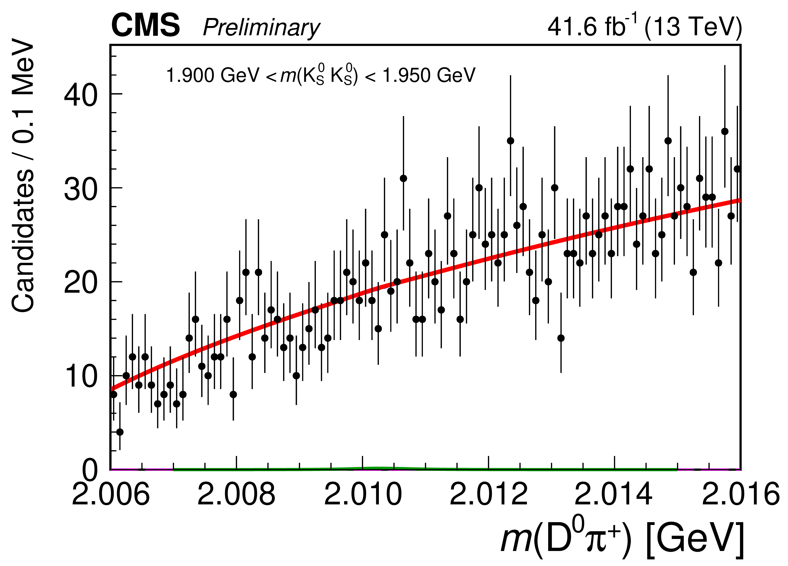
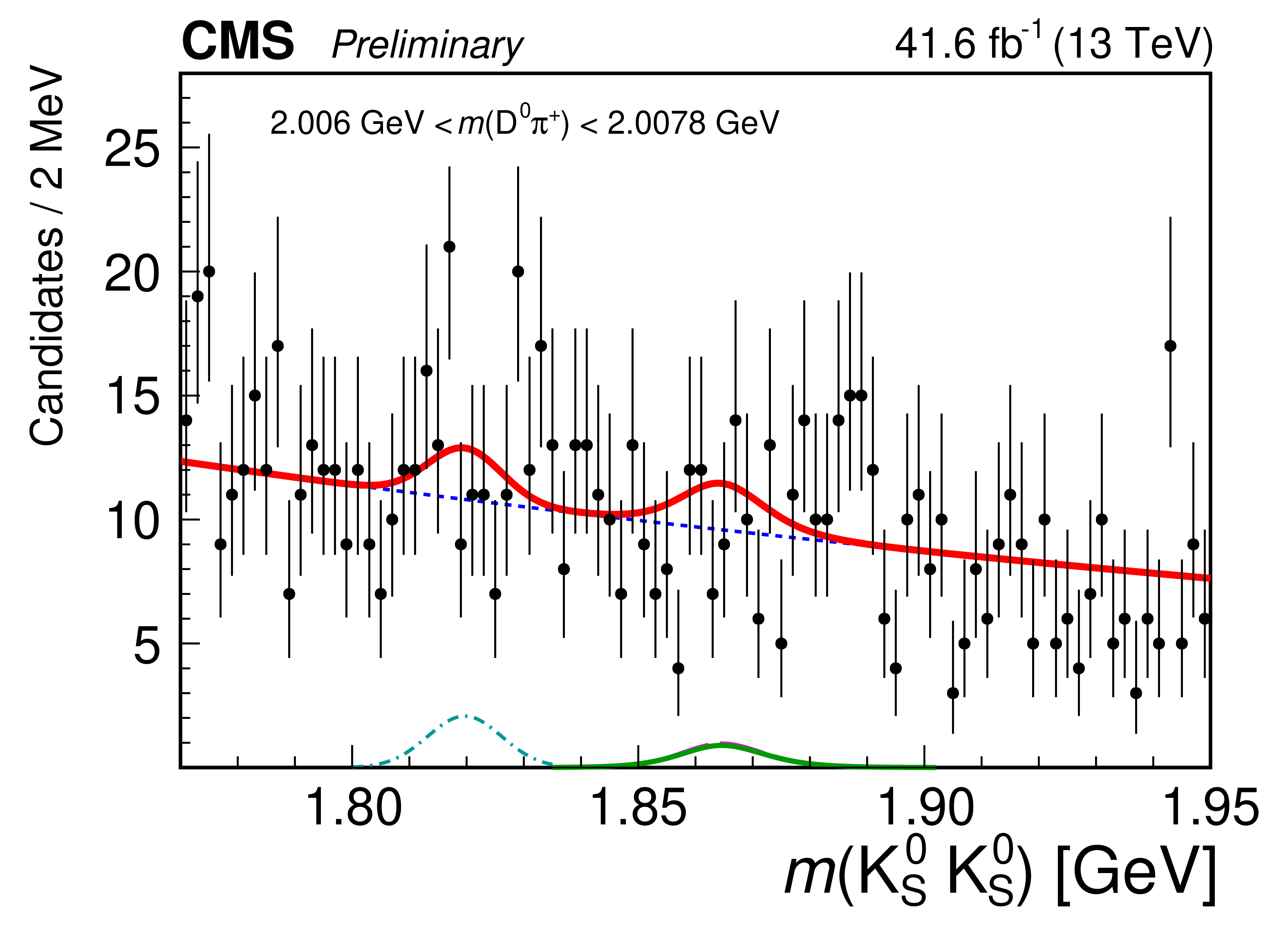
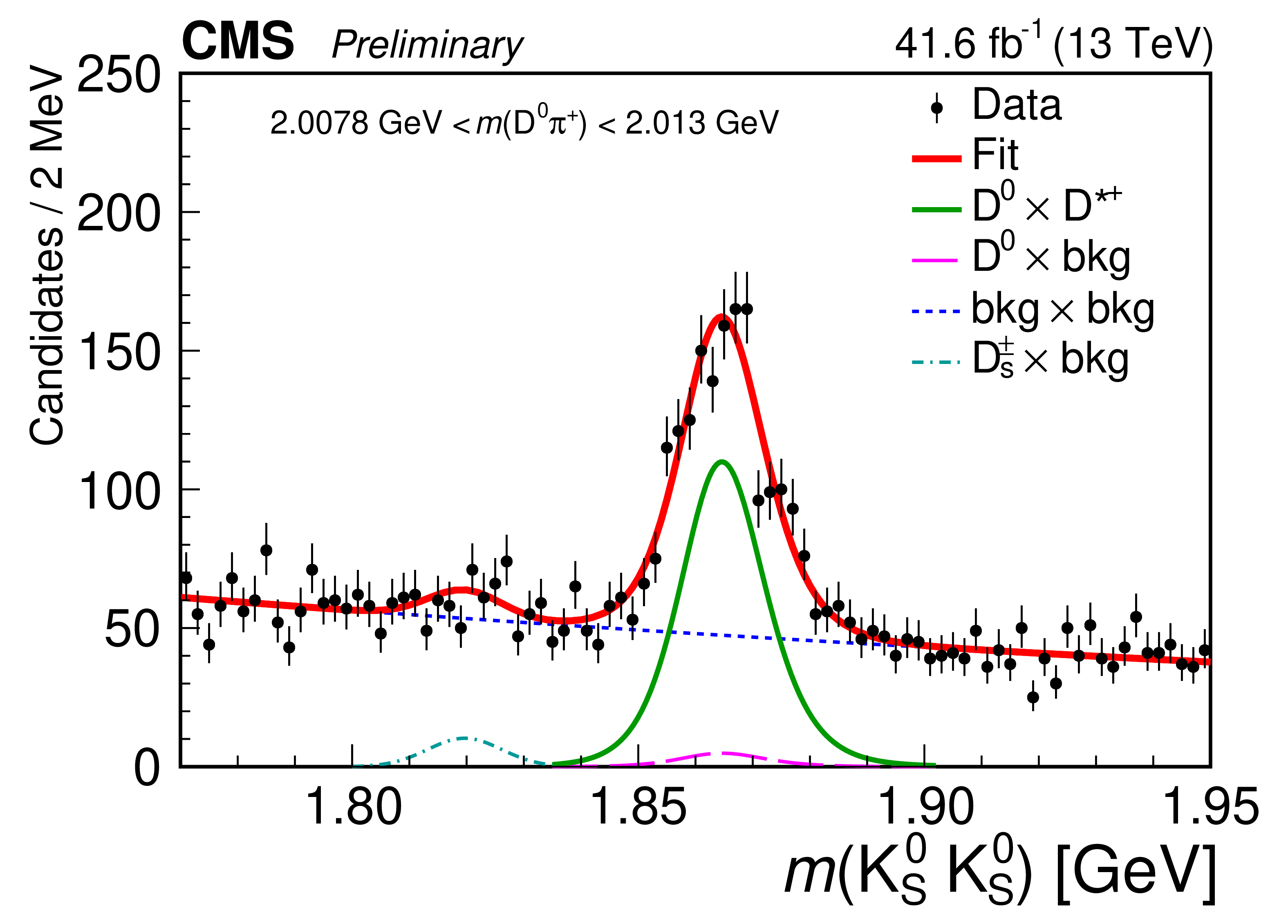
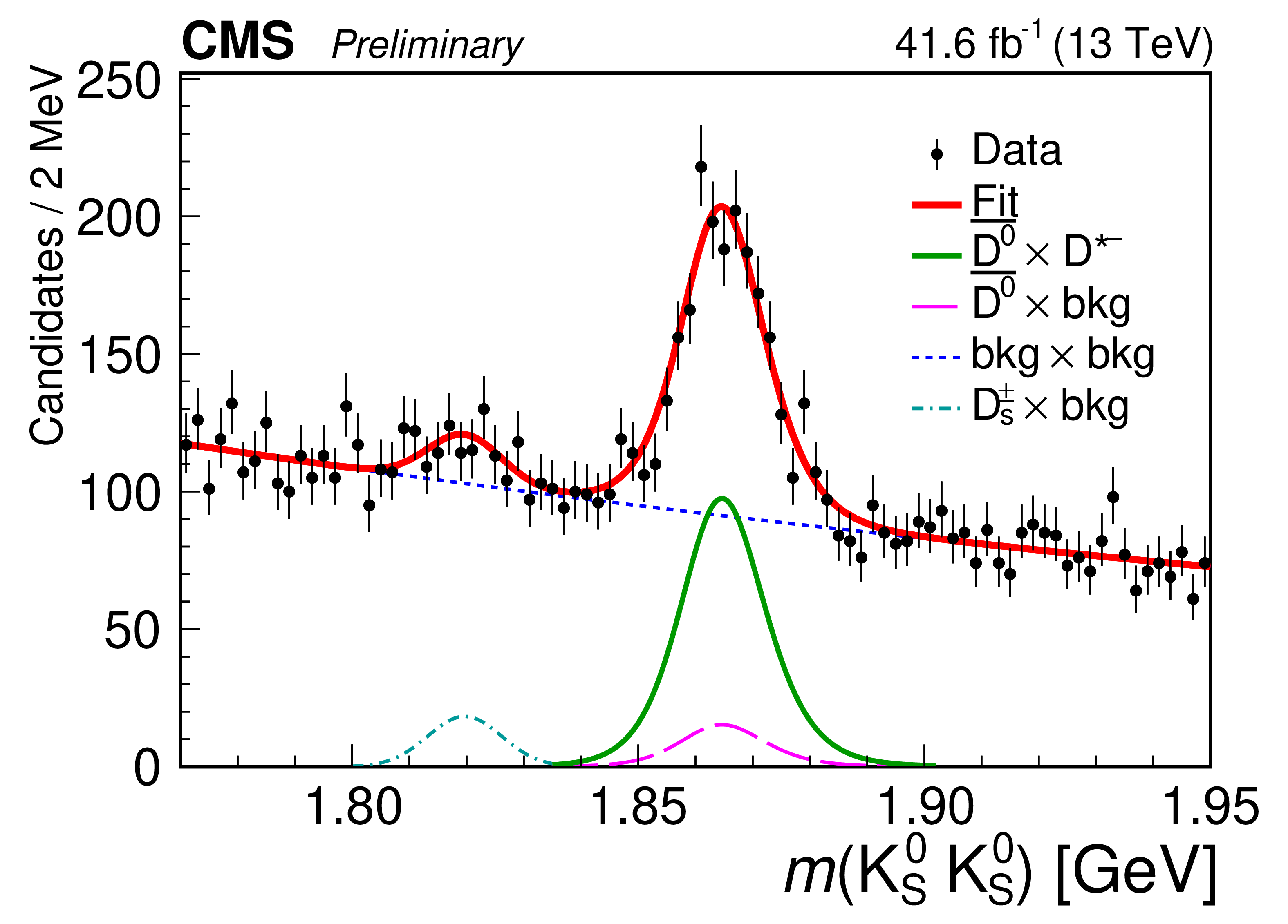
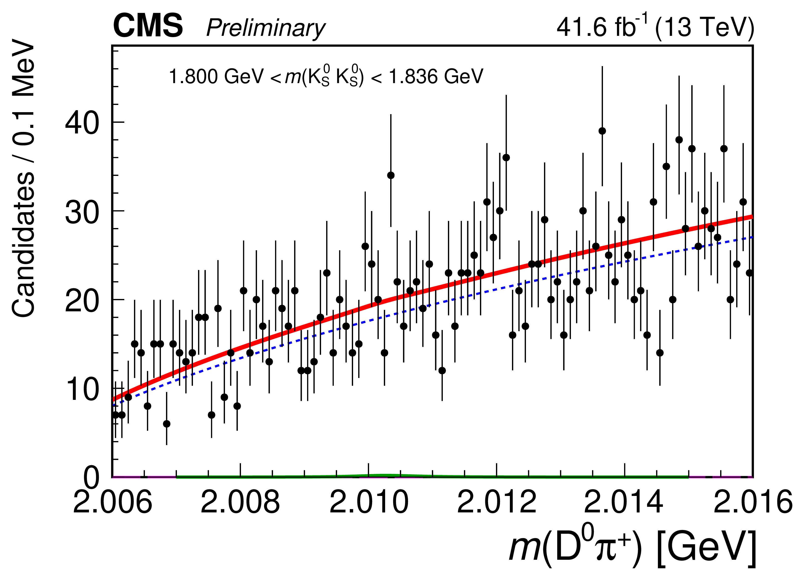
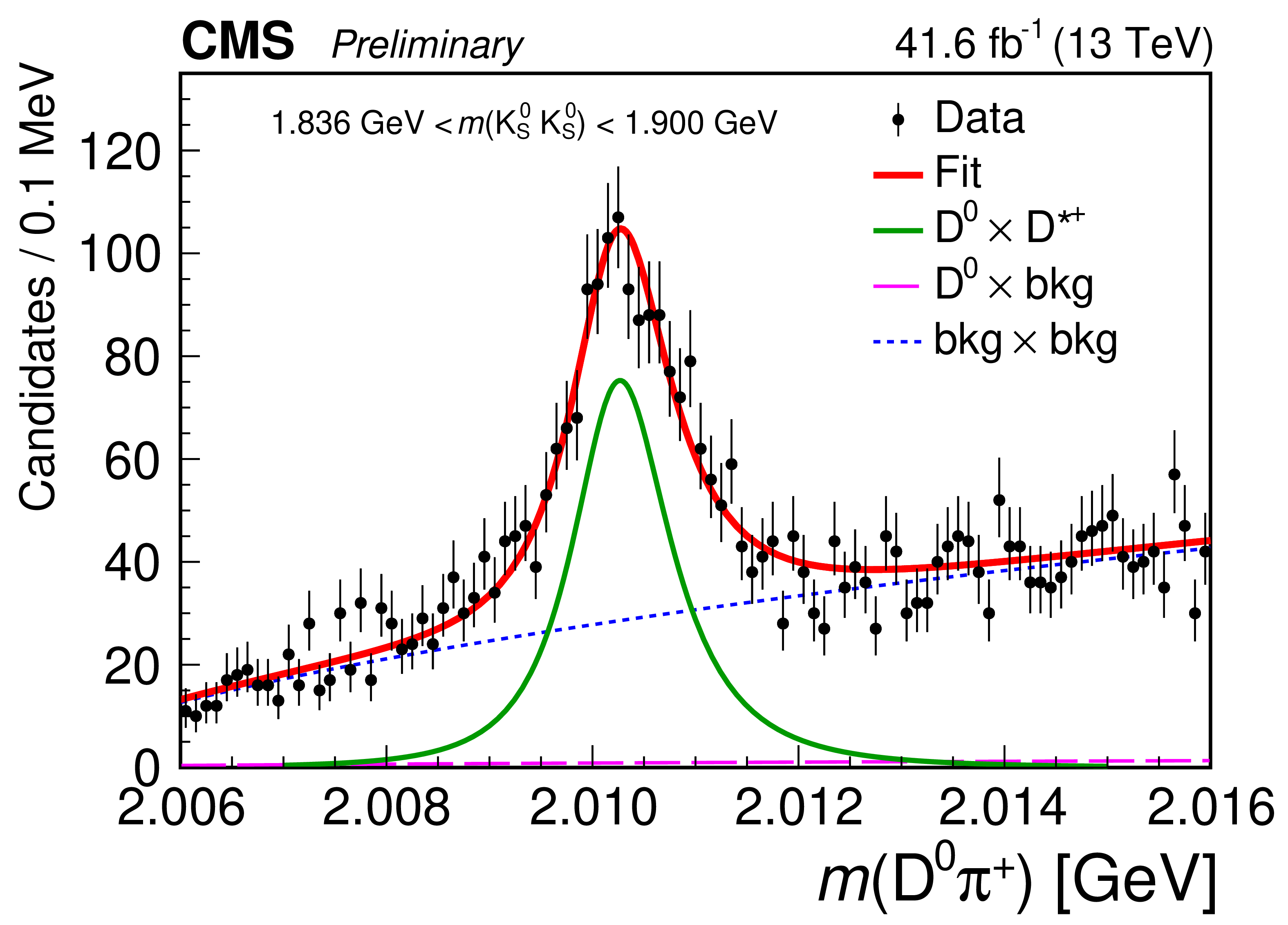
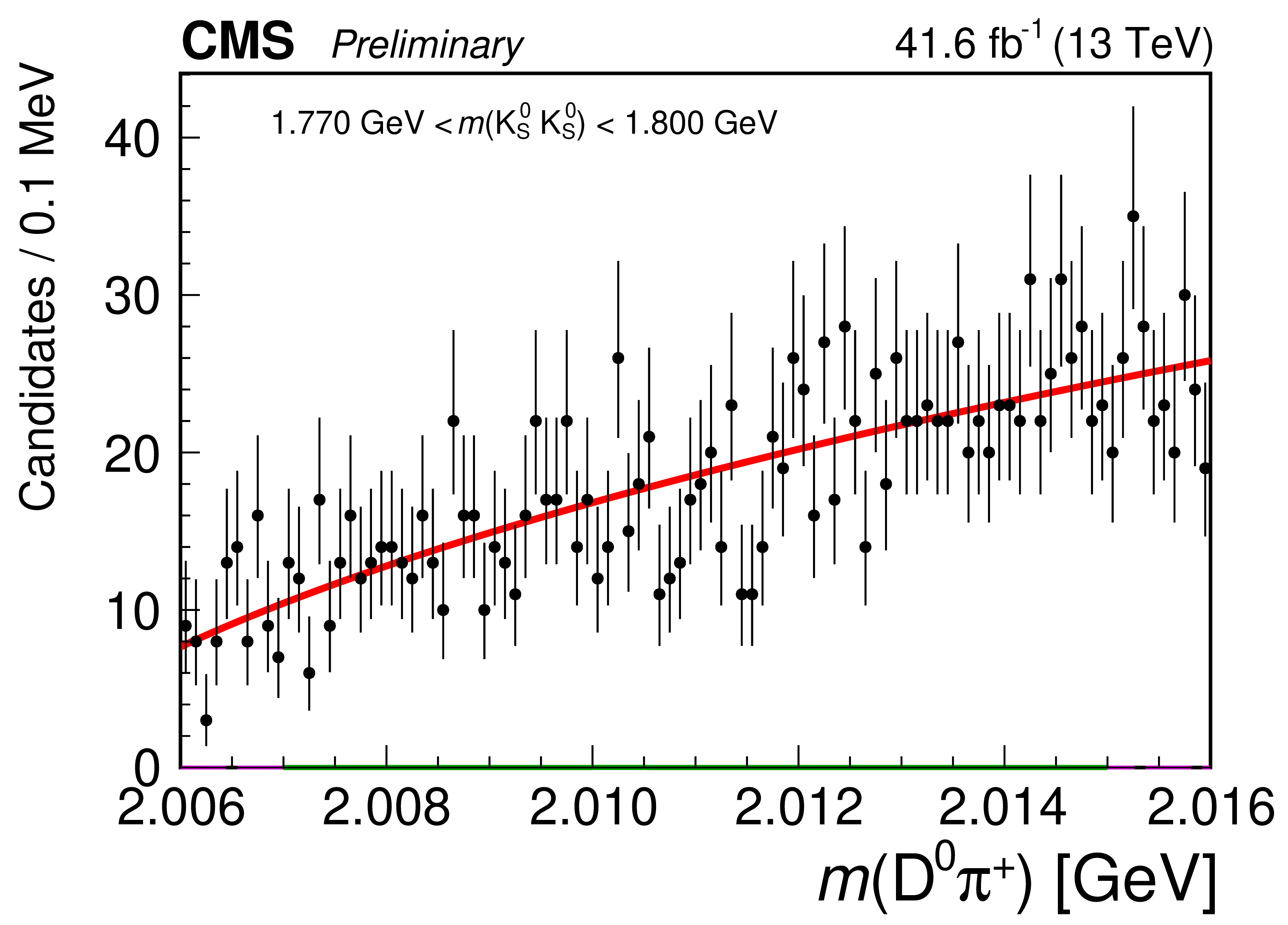
png pdf	Figure 4: Results of the 2D fit to $m(\mathrm{D}\pi^{\pm}):m(\mathrm{K^0_S}\mathrm{K^0_S})$ for the signal channel in measured data, $\mathrm{D}^{*+}$ candidates. Top row: the projections of the 2D fit on $m(\mathrm{D}\pi^{\pm})$ in the ranges of $m(\mathrm{K^0_S}\mathrm{K^0_S})$: region of $\mathrm{D}_{s}^{\pm}\to\mathrm{K^0_S}\mathrm{K^0_S}\pi^{\pm}$ contamination (left) and signal region of $\mathrm{K^0_S}\mathrm{K^0_S}$ (right). Middle row: projections of the 2D fit on $m(\mathrm{D}\pi^{\pm})$ in the ranges of $m(\mathrm{K^0_S}\mathrm{K^0_S})$: left sideband (left) and right sideband (right). Bottom row: projections of the 2D fit on $m(\mathrm{K^0_S}\mathrm{K^0_S})$ in the ranges of $m(\mathrm{D}\pi^{\pm})$: left sideband (left), signal region of $\mathrm{D^0}\pi^{+}$ (center), and right sideband (right). The green line corresponds to the signal component, the blue short-dashed line shows the combinatorial background, the purple long-dashed line shows the combinations of $\mathrm{D^0}$ with background pions, and the magenta dash-dotted line illustrates the contamination of $\mathrm{D}_{s}^{\pm}\to\mathrm{K^0_S}\mathrm{K^0_S}\pi^{\pm}$ decay.
png pdf	Figure 4-a: Results of the 2D fit to $m(\mathrm{D}\pi^{\pm}):m(\mathrm{K^0_S}\mathrm{K^0_S})$ for the signal channel in measured data, $\mathrm{D}^{*+}$ candidates. Top row: the projections of the 2D fit on $m(\mathrm{D}\pi^{\pm})$ in the ranges of $m(\mathrm{K^0_S}\mathrm{K^0_S})$: region of $\mathrm{D}_{s}^{\pm}\to\mathrm{K^0_S}\mathrm{K^0_S}\pi^{\pm}$ contamination (left) and signal region of $\mathrm{K^0_S}\mathrm{K^0_S}$ (right). Middle row: projections of the 2D fit on $m(\mathrm{D}\pi^{\pm})$ in the ranges of $m(\mathrm{K^0_S}\mathrm{K^0_S})$: left sideband (left) and right sideband (right). Bottom row: projections of the 2D fit on $m(\mathrm{K^0_S}\mathrm{K^0_S})$ in the ranges of $m(\mathrm{D}\pi^{\pm})$: left sideband (left), signal region of $\mathrm{D^0}\pi^{+}$ (center), and right sideband (right). The green line corresponds to the signal component, the blue short-dashed line shows the combinatorial background, the purple long-dashed line shows the combinations of $\mathrm{D^0}$ with background pions, and the magenta dash-dotted line illustrates the contamination of $\mathrm{D}_{s}^{\pm}\to\mathrm{K^0_S}\mathrm{K^0_S}\pi^{\pm}$ decay.
png pdf	Figure 4-b: Results of the 2D fit to $m(\mathrm{D}\pi^{\pm}):m(\mathrm{K^0_S}\mathrm{K^0_S})$ for the signal channel in measured data, $\mathrm{D}^{*+}$ candidates. Top row: the projections of the 2D fit on $m(\mathrm{D}\pi^{\pm})$ in the ranges of $m(\mathrm{K^0_S}\mathrm{K^0_S})$: region of $\mathrm{D}_{s}^{\pm}\to\mathrm{K^0_S}\mathrm{K^0_S}\pi^{\pm}$ contamination (left) and signal region of $\mathrm{K^0_S}\mathrm{K^0_S}$ (right). Middle row: projections of the 2D fit on $m(\mathrm{D}\pi^{\pm})$ in the ranges of $m(\mathrm{K^0_S}\mathrm{K^0_S})$: left sideband (left) and right sideband (right). Bottom row: projections of the 2D fit on $m(\mathrm{K^0_S}\mathrm{K^0_S})$ in the ranges of $m(\mathrm{D}\pi^{\pm})$: left sideband (left), signal region of $\mathrm{D^0}\pi^{+}$ (center), and right sideband (right). The green line corresponds to the signal component, the blue short-dashed line shows the combinatorial background, the purple long-dashed line shows the combinations of $\mathrm{D^0}$ with background pions, and the magenta dash-dotted line illustrates the contamination of $\mathrm{D}_{s}^{\pm}\to\mathrm{K^0_S}\mathrm{K^0_S}\pi^{\pm}$ decay.
png pdf	Figure 4-c: Results of the 2D fit to $m(\mathrm{D}\pi^{\pm}):m(\mathrm{K^0_S}\mathrm{K^0_S})$ for the signal channel in measured data, $\mathrm{D}^{*+}$ candidates. Top row: the projections of the 2D fit on $m(\mathrm{D}\pi^{\pm})$ in the ranges of $m(\mathrm{K^0_S}\mathrm{K^0_S})$: region of $\mathrm{D}_{s}^{\pm}\to\mathrm{K^0_S}\mathrm{K^0_S}\pi^{\pm}$ contamination (left) and signal region of $\mathrm{K^0_S}\mathrm{K^0_S}$ (right). Middle row: projections of the 2D fit on $m(\mathrm{D}\pi^{\pm})$ in the ranges of $m(\mathrm{K^0_S}\mathrm{K^0_S})$: left sideband (left) and right sideband (right). Bottom row: projections of the 2D fit on $m(\mathrm{K^0_S}\mathrm{K^0_S})$ in the ranges of $m(\mathrm{D}\pi^{\pm})$: left sideband (left), signal region of $\mathrm{D^0}\pi^{+}$ (center), and right sideband (right). The green line corresponds to the signal component, the blue short-dashed line shows the combinatorial background, the purple long-dashed line shows the combinations of $\mathrm{D^0}$ with background pions, and the magenta dash-dotted line illustrates the contamination of $\mathrm{D}_{s}^{\pm}\to\mathrm{K^0_S}\mathrm{K^0_S}\pi^{\pm}$ decay.
png pdf	Figure 4-d: Results of the 2D fit to $m(\mathrm{D}\pi^{\pm}):m(\mathrm{K^0_S}\mathrm{K^0_S})$ for the signal channel in measured data, $\mathrm{D}^{*+}$ candidates. Top row: the projections of the 2D fit on $m(\mathrm{D}\pi^{\pm})$ in the ranges of $m(\mathrm{K^0_S}\mathrm{K^0_S})$: region of $\mathrm{D}_{s}^{\pm}\to\mathrm{K^0_S}\mathrm{K^0_S}\pi^{\pm}$ contamination (left) and signal region of $\mathrm{K^0_S}\mathrm{K^0_S}$ (right). Middle row: projections of the 2D fit on $m(\mathrm{D}\pi^{\pm})$ in the ranges of $m(\mathrm{K^0_S}\mathrm{K^0_S})$: left sideband (left) and right sideband (right). Bottom row: projections of the 2D fit on $m(\mathrm{K^0_S}\mathrm{K^0_S})$ in the ranges of $m(\mathrm{D}\pi^{\pm})$: left sideband (left), signal region of $\mathrm{D^0}\pi^{+}$ (center), and right sideband (right). The green line corresponds to the signal component, the blue short-dashed line shows the combinatorial background, the purple long-dashed line shows the combinations of $\mathrm{D^0}$ with background pions, and the magenta dash-dotted line illustrates the contamination of $\mathrm{D}_{s}^{\pm}\to\mathrm{K^0_S}\mathrm{K^0_S}\pi^{\pm}$ decay.
png pdf	Figure 4-e: Results of the 2D fit to $m(\mathrm{D}\pi^{\pm}):m(\mathrm{K^0_S}\mathrm{K^0_S})$ for the signal channel in measured data, $\mathrm{D}^{*+}$ candidates. Top row: the projections of the 2D fit on $m(\mathrm{D}\pi^{\pm})$ in the ranges of $m(\mathrm{K^0_S}\mathrm{K^0_S})$: region of $\mathrm{D}_{s}^{\pm}\to\mathrm{K^0_S}\mathrm{K^0_S}\pi^{\pm}$ contamination (left) and signal region of $\mathrm{K^0_S}\mathrm{K^0_S}$ (right). Middle row: projections of the 2D fit on $m(\mathrm{D}\pi^{\pm})$ in the ranges of $m(\mathrm{K^0_S}\mathrm{K^0_S})$: left sideband (left) and right sideband (right). Bottom row: projections of the 2D fit on $m(\mathrm{K^0_S}\mathrm{K^0_S})$ in the ranges of $m(\mathrm{D}\pi^{\pm})$: left sideband (left), signal region of $\mathrm{D^0}\pi^{+}$ (center), and right sideband (right). The green line corresponds to the signal component, the blue short-dashed line shows the combinatorial background, the purple long-dashed line shows the combinations of $\mathrm{D^0}$ with background pions, and the magenta dash-dotted line illustrates the contamination of $\mathrm{D}_{s}^{\pm}\to\mathrm{K^0_S}\mathrm{K^0_S}\pi^{\pm}$ decay.
png pdf	Figure 4-f: Results of the 2D fit to $m(\mathrm{D}\pi^{\pm}):m(\mathrm{K^0_S}\mathrm{K^0_S})$ for the signal channel in measured data, $\mathrm{D}^{*+}$ candidates. Top row: the projections of the 2D fit on $m(\mathrm{D}\pi^{\pm})$ in the ranges of $m(\mathrm{K^0_S}\mathrm{K^0_S})$: region of $\mathrm{D}_{s}^{\pm}\to\mathrm{K^0_S}\mathrm{K^0_S}\pi^{\pm}$ contamination (left) and signal region of $\mathrm{K^0_S}\mathrm{K^0_S}$ (right). Middle row: projections of the 2D fit on $m(\mathrm{D}\pi^{\pm})$ in the ranges of $m(\mathrm{K^0_S}\mathrm{K^0_S})$: left sideband (left) and right sideband (right). Bottom row: projections of the 2D fit on $m(\mathrm{K^0_S}\mathrm{K^0_S})$ in the ranges of $m(\mathrm{D}\pi^{\pm})$: left sideband (left), signal region of $\mathrm{D^0}\pi^{+}$ (center), and right sideband (right). The green line corresponds to the signal component, the blue short-dashed line shows the combinatorial background, the purple long-dashed line shows the combinations of $\mathrm{D^0}$ with background pions, and the magenta dash-dotted line illustrates the contamination of $\mathrm{D}_{s}^{\pm}\to\mathrm{K^0_S}\mathrm{K^0_S}\pi^{\pm}$ decay.
png pdf	Figure 4-g: Results of the 2D fit to $m(\mathrm{D}\pi^{\pm}):m(\mathrm{K^0_S}\mathrm{K^0_S})$ for the signal channel in measured data, $\mathrm{D}^{*+}$ candidates. Top row: the projections of the 2D fit on $m(\mathrm{D}\pi^{\pm})$ in the ranges of $m(\mathrm{K^0_S}\mathrm{K^0_S})$: region of $\mathrm{D}_{s}^{\pm}\to\mathrm{K^0_S}\mathrm{K^0_S}\pi^{\pm}$ contamination (left) and signal region of $\mathrm{K^0_S}\mathrm{K^0_S}$ (right). Middle row: projections of the 2D fit on $m(\mathrm{D}\pi^{\pm})$ in the ranges of $m(\mathrm{K^0_S}\mathrm{K^0_S})$: left sideband (left) and right sideband (right). Bottom row: projections of the 2D fit on $m(\mathrm{K^0_S}\mathrm{K^0_S})$ in the ranges of $m(\mathrm{D}\pi^{\pm})$: left sideband (left), signal region of $\mathrm{D^0}\pi^{+}$ (center), and right sideband (right). The green line corresponds to the signal component, the blue short-dashed line shows the combinatorial background, the purple long-dashed line shows the combinations of $\mathrm{D^0}$ with background pions, and the magenta dash-dotted line illustrates the contamination of $\mathrm{D}_{s}^{\pm}\to\mathrm{K^0_S}\mathrm{K^0_S}\pi^{\pm}$ decay.
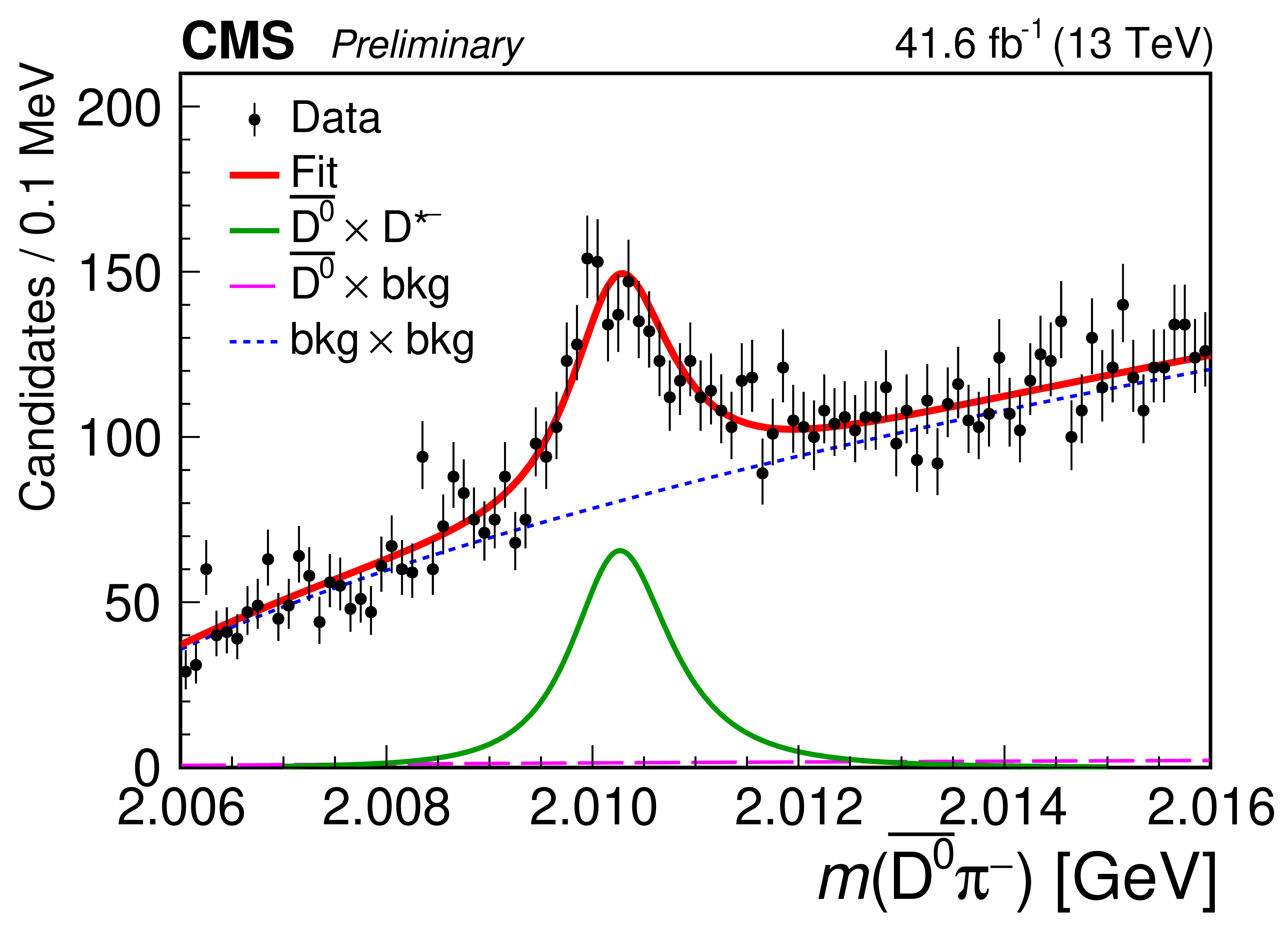
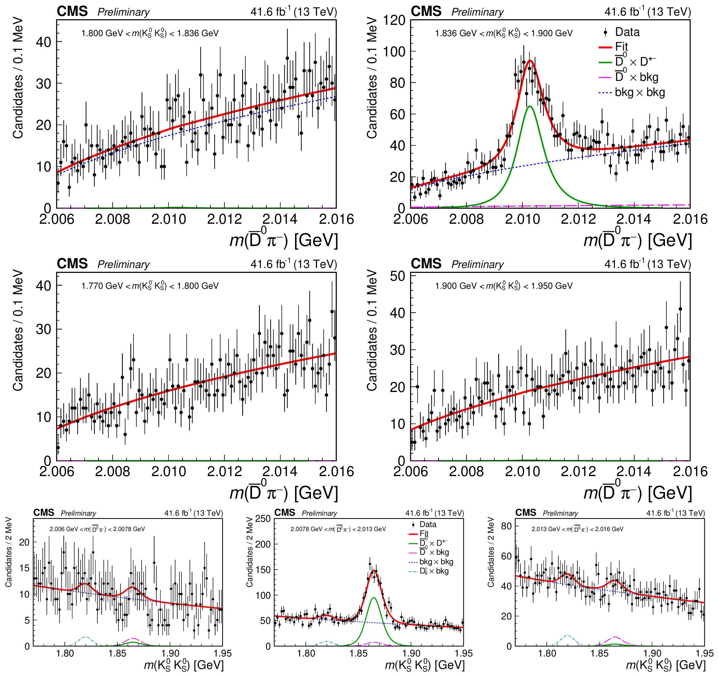
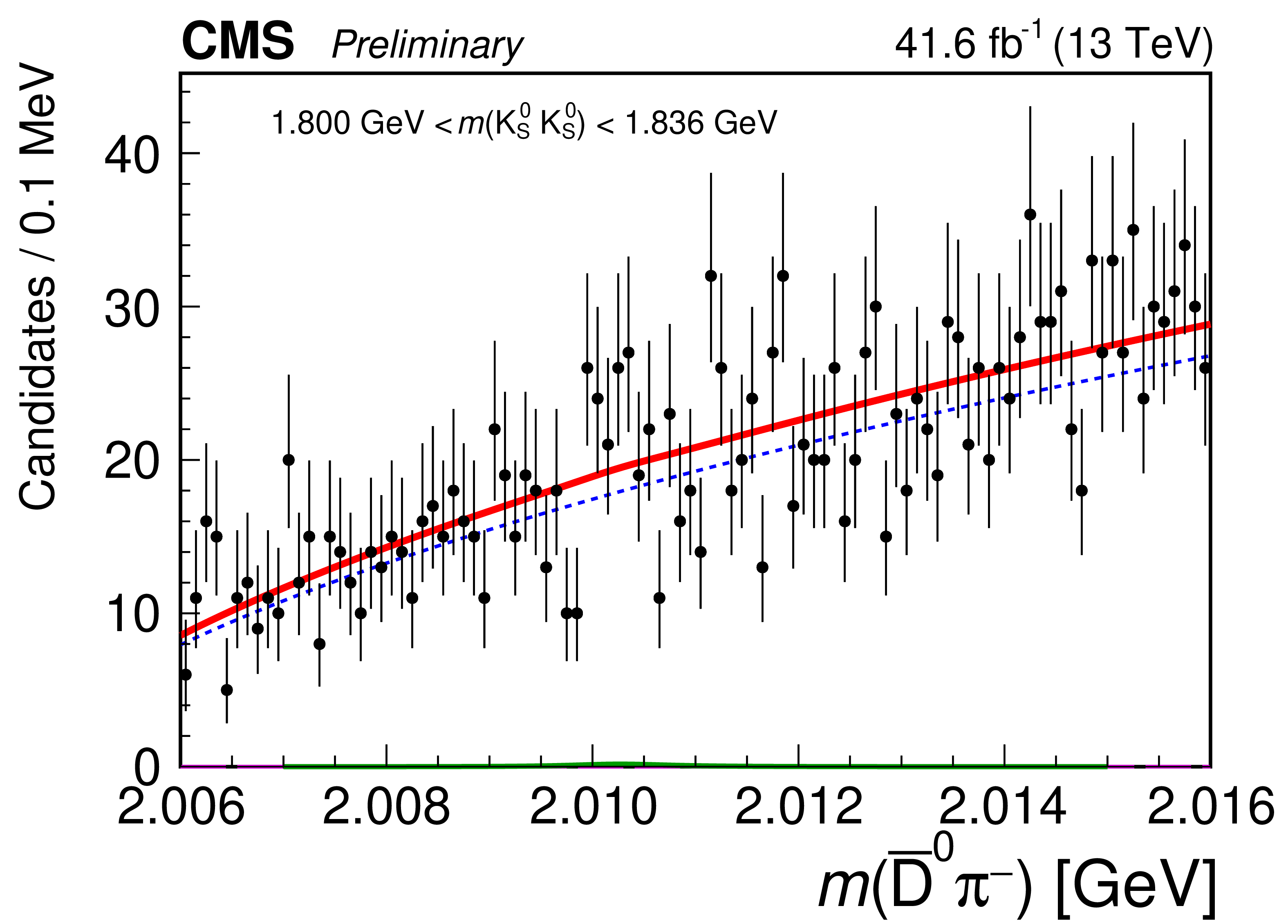
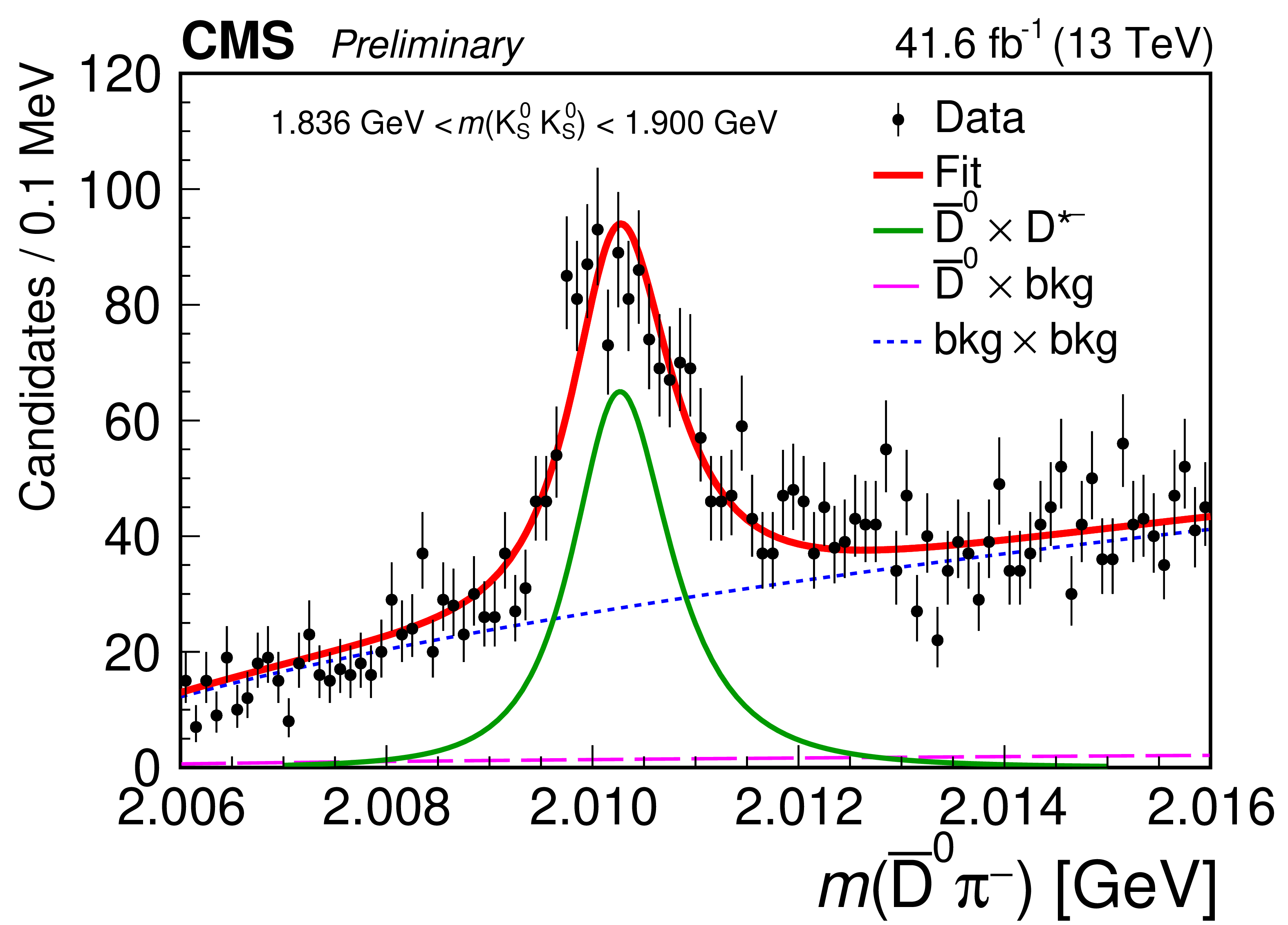
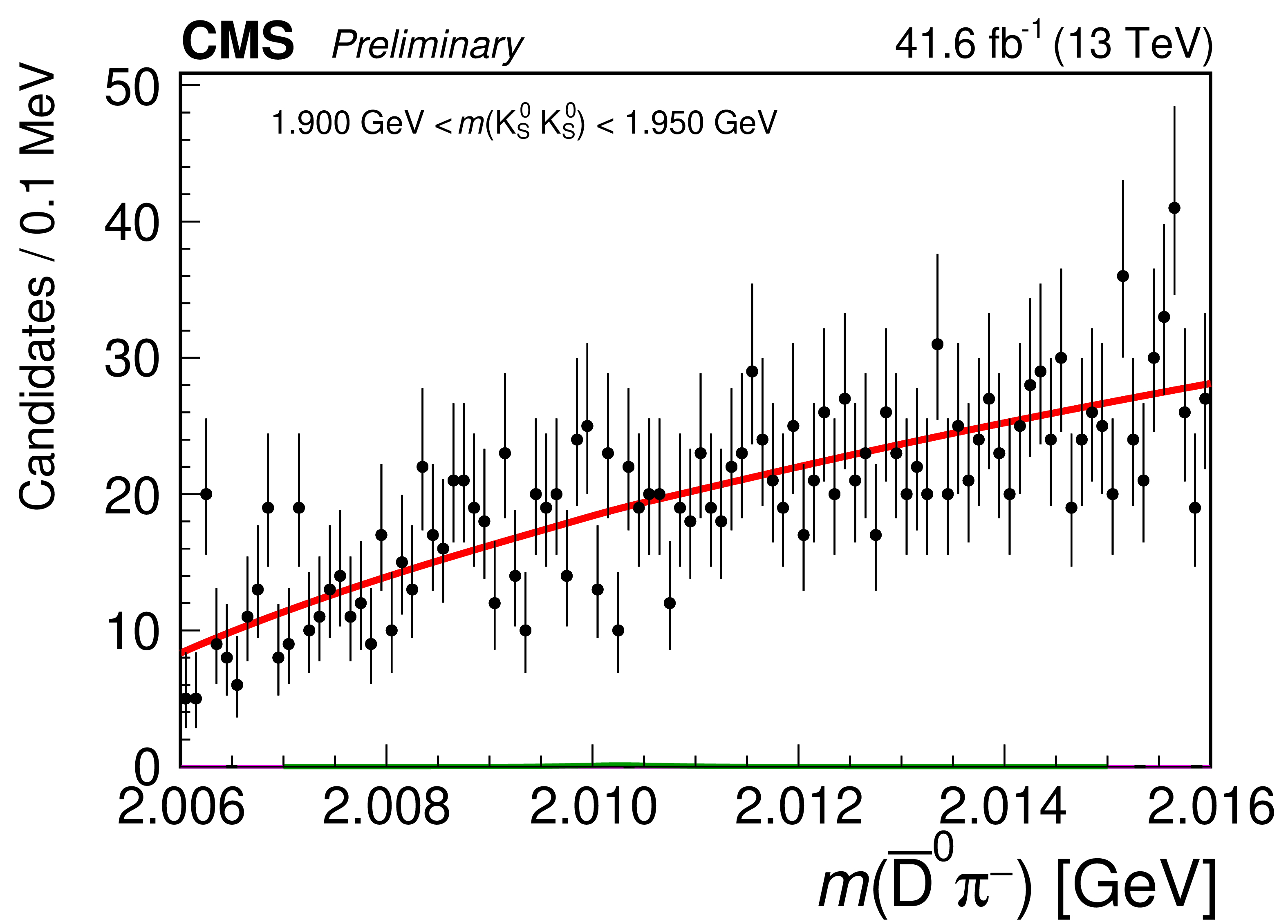
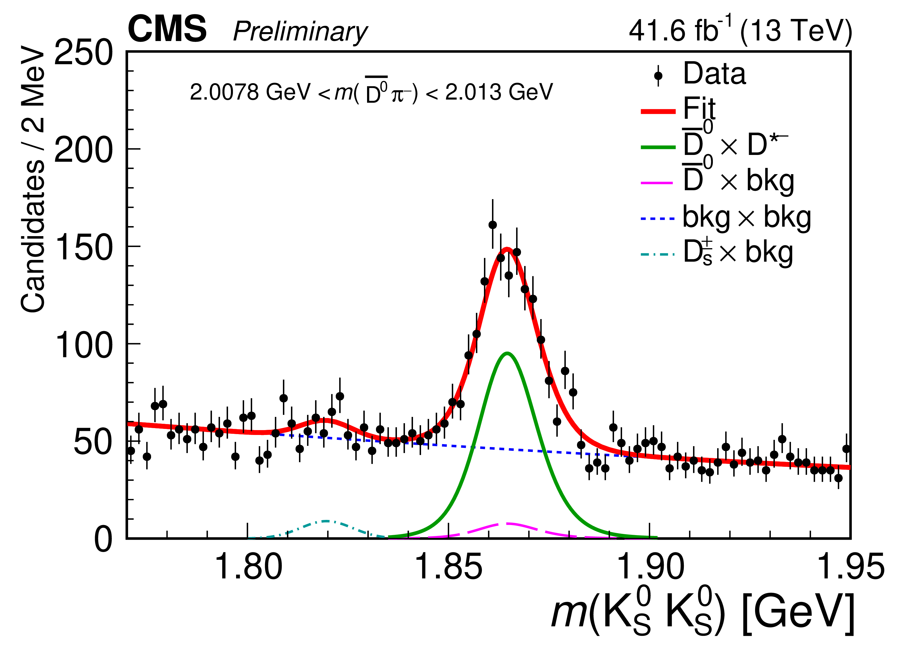
png pdf	Figure 5: Results of the 2D fit to $m(\mathrm{D}\pi^{\pm}):m(\mathrm{K^0_S}\mathrm{K^0_S})$ for the signal channel in measured data, $\mathrm{D}^{*-}$ candidates. Top row: the projections of the 2D fit on $m(\mathrm{D}\pi^{\pm})$ in the ranges of $m(\mathrm{K^0_S}\mathrm{K^0_S})$: region of $\mathrm{D}_{s}^{\pm}\to\mathrm{K^0_S}\mathrm{K^0_S}\pi^{\pm}$ contamination (left) and signal region of $\mathrm{K^0_S}\mathrm{K^0_S}$ (right). Middle row: projections of the 2D fit on $m(\mathrm{D}\pi^{\pm})$ in the ranges of $m(\mathrm{K^0_S}\mathrm{K^0_S})$: left sideband (left) and right sideband (right). Bottom row: projections of the 2D fit on $m(\mathrm{K^0_S}\mathrm{K^0_S})$ in the ranges of $m(\mathrm{D}\pi^{\pm})$: left sideband (left), signal region of $\overline{\mathrm{D}}^{0}\pi^{-}$ (center), and right sideband (right). The green line corresponds to the signal component, the blue short-dashed line shows the combinatorial background, the purple long-dashed line shows the combinations of $\overline{\mathrm{D}}^{0}$ with background pions, and the magenta dash-dotted line illustrates the contamination of $\mathrm{D}_{s}^{\pm}\to\mathrm{K^0_S}\mathrm{K^0_S}\pi^{\pm}$ decay.
png pdf	Figure 5-a: Results of the 2D fit to $m(\mathrm{D}\pi^{\pm}):m(\mathrm{K^0_S}\mathrm{K^0_S})$ for the signal channel in measured data, $\mathrm{D}^{*-}$ candidates. Top row: the projections of the 2D fit on $m(\mathrm{D}\pi^{\pm})$ in the ranges of $m(\mathrm{K^0_S}\mathrm{K^0_S})$: region of $\mathrm{D}_{s}^{\pm}\to\mathrm{K^0_S}\mathrm{K^0_S}\pi^{\pm}$ contamination (left) and signal region of $\mathrm{K^0_S}\mathrm{K^0_S}$ (right). Middle row: projections of the 2D fit on $m(\mathrm{D}\pi^{\pm})$ in the ranges of $m(\mathrm{K^0_S}\mathrm{K^0_S})$: left sideband (left) and right sideband (right). Bottom row: projections of the 2D fit on $m(\mathrm{K^0_S}\mathrm{K^0_S})$ in the ranges of $m(\mathrm{D}\pi^{\pm})$: left sideband (left), signal region of $\overline{\mathrm{D}}^{0}\pi^{-}$ (center), and right sideband (right). The green line corresponds to the signal component, the blue short-dashed line shows the combinatorial background, the purple long-dashed line shows the combinations of $\overline{\mathrm{D}}^{0}$ with background pions, and the magenta dash-dotted line illustrates the contamination of $\mathrm{D}_{s}^{\pm}\to\mathrm{K^0_S}\mathrm{K^0_S}\pi^{\pm}$ decay.
png pdf	Figure 5-b: Results of the 2D fit to $m(\mathrm{D}\pi^{\pm}):m(\mathrm{K^0_S}\mathrm{K^0_S})$ for the signal channel in measured data, $\mathrm{D}^{*-}$ candidates. Top row: the projections of the 2D fit on $m(\mathrm{D}\pi^{\pm})$ in the ranges of $m(\mathrm{K^0_S}\mathrm{K^0_S})$: region of $\mathrm{D}_{s}^{\pm}\to\mathrm{K^0_S}\mathrm{K^0_S}\pi^{\pm}$ contamination (left) and signal region of $\mathrm{K^0_S}\mathrm{K^0_S}$ (right). Middle row: projections of the 2D fit on $m(\mathrm{D}\pi^{\pm})$ in the ranges of $m(\mathrm{K^0_S}\mathrm{K^0_S})$: left sideband (left) and right sideband (right). Bottom row: projections of the 2D fit on $m(\mathrm{K^0_S}\mathrm{K^0_S})$ in the ranges of $m(\mathrm{D}\pi^{\pm})$: left sideband (left), signal region of $\overline{\mathrm{D}}^{0}\pi^{-}$ (center), and right sideband (right). The green line corresponds to the signal component, the blue short-dashed line shows the combinatorial background, the purple long-dashed line shows the combinations of $\overline{\mathrm{D}}^{0}$ with background pions, and the magenta dash-dotted line illustrates the contamination of $\mathrm{D}_{s}^{\pm}\to\mathrm{K^0_S}\mathrm{K^0_S}\pi^{\pm}$ decay.
png pdf	Figure 5-c: Results of the 2D fit to $m(\mathrm{D}\pi^{\pm}):m(\mathrm{K^0_S}\mathrm{K^0_S})$ for the signal channel in measured data, $\mathrm{D}^{*-}$ candidates. Top row: the projections of the 2D fit on $m(\mathrm{D}\pi^{\pm})$ in the ranges of $m(\mathrm{K^0_S}\mathrm{K^0_S})$: region of $\mathrm{D}_{s}^{\pm}\to\mathrm{K^0_S}\mathrm{K^0_S}\pi^{\pm}$ contamination (left) and signal region of $\mathrm{K^0_S}\mathrm{K^0_S}$ (right). Middle row: projections of the 2D fit on $m(\mathrm{D}\pi^{\pm})$ in the ranges of $m(\mathrm{K^0_S}\mathrm{K^0_S})$: left sideband (left) and right sideband (right). Bottom row: projections of the 2D fit on $m(\mathrm{K^0_S}\mathrm{K^0_S})$ in the ranges of $m(\mathrm{D}\pi^{\pm})$: left sideband (left), signal region of $\overline{\mathrm{D}}^{0}\pi^{-}$ (center), and right sideband (right). The green line corresponds to the signal component, the blue short-dashed line shows the combinatorial background, the purple long-dashed line shows the combinations of $\overline{\mathrm{D}}^{0}$ with background pions, and the magenta dash-dotted line illustrates the contamination of $\mathrm{D}_{s}^{\pm}\to\mathrm{K^0_S}\mathrm{K^0_S}\pi^{\pm}$ decay.
png pdf	Figure 5-d: Results of the 2D fit to $m(\mathrm{D}\pi^{\pm}):m(\mathrm{K^0_S}\mathrm{K^0_S})$ for the signal channel in measured data, $\mathrm{D}^{*-}$ candidates. Top row: the projections of the 2D fit on $m(\mathrm{D}\pi^{\pm})$ in the ranges of $m(\mathrm{K^0_S}\mathrm{K^0_S})$: region of $\mathrm{D}_{s}^{\pm}\to\mathrm{K^0_S}\mathrm{K^0_S}\pi^{\pm}$ contamination (left) and signal region of $\mathrm{K^0_S}\mathrm{K^0_S}$ (right). Middle row: projections of the 2D fit on $m(\mathrm{D}\pi^{\pm})$ in the ranges of $m(\mathrm{K^0_S}\mathrm{K^0_S})$: left sideband (left) and right sideband (right). Bottom row: projections of the 2D fit on $m(\mathrm{K^0_S}\mathrm{K^0_S})$ in the ranges of $m(\mathrm{D}\pi^{\pm})$: left sideband (left), signal region of $\overline{\mathrm{D}}^{0}\pi^{-}$ (center), and right sideband (right). The green line corresponds to the signal component, the blue short-dashed line shows the combinatorial background, the purple long-dashed line shows the combinations of $\overline{\mathrm{D}}^{0}$ with background pions, and the magenta dash-dotted line illustrates the contamination of $\mathrm{D}_{s}^{\pm}\to\mathrm{K^0_S}\mathrm{K^0_S}\pi^{\pm}$ decay.
png pdf	Figure 5-e: Results of the 2D fit to $m(\mathrm{D}\pi^{\pm}):m(\mathrm{K^0_S}\mathrm{K^0_S})$ for the signal channel in measured data, $\mathrm{D}^{*-}$ candidates. Top row: the projections of the 2D fit on $m(\mathrm{D}\pi^{\pm})$ in the ranges of $m(\mathrm{K^0_S}\mathrm{K^0_S})$: region of $\mathrm{D}_{s}^{\pm}\to\mathrm{K^0_S}\mathrm{K^0_S}\pi^{\pm}$ contamination (left) and signal region of $\mathrm{K^0_S}\mathrm{K^0_S}$ (right). Middle row: projections of the 2D fit on $m(\mathrm{D}\pi^{\pm})$ in the ranges of $m(\mathrm{K^0_S}\mathrm{K^0_S})$: left sideband (left) and right sideband (right). Bottom row: projections of the 2D fit on $m(\mathrm{K^0_S}\mathrm{K^0_S})$ in the ranges of $m(\mathrm{D}\pi^{\pm})$: left sideband (left), signal region of $\overline{\mathrm{D}}^{0}\pi^{-}$ (center), and right sideband (right). The green line corresponds to the signal component, the blue short-dashed line shows the combinatorial background, the purple long-dashed line shows the combinations of $\overline{\mathrm{D}}^{0}$ with background pions, and the magenta dash-dotted line illustrates the contamination of $\mathrm{D}_{s}^{\pm}\to\mathrm{K^0_S}\mathrm{K^0_S}\pi^{\pm}$ decay.
png pdf	Figure 5-f: Results of the 2D fit to $m(\mathrm{D}\pi^{\pm}):m(\mathrm{K^0_S}\mathrm{K^0_S})$ for the signal channel in measured data, $\mathrm{D}^{*-}$ candidates. Top row: the projections of the 2D fit on $m(\mathrm{D}\pi^{\pm})$ in the ranges of $m(\mathrm{K^0_S}\mathrm{K^0_S})$: region of $\mathrm{D}_{s}^{\pm}\to\mathrm{K^0_S}\mathrm{K^0_S}\pi^{\pm}$ contamination (left) and signal region of $\mathrm{K^0_S}\mathrm{K^0_S}$ (right). Middle row: projections of the 2D fit on $m(\mathrm{D}\pi^{\pm})$ in the ranges of $m(\mathrm{K^0_S}\mathrm{K^0_S})$: left sideband (left) and right sideband (right). Bottom row: projections of the 2D fit on $m(\mathrm{K^0_S}\mathrm{K^0_S})$ in the ranges of $m(\mathrm{D}\pi^{\pm})$: left sideband (left), signal region of $\overline{\mathrm{D}}^{0}\pi^{-}$ (center), and right sideband (right). The green line corresponds to the signal component, the blue short-dashed line shows the combinatorial background, the purple long-dashed line shows the combinations of $\overline{\mathrm{D}}^{0}$ with background pions, and the magenta dash-dotted line illustrates the contamination of $\mathrm{D}_{s}^{\pm}\to\mathrm{K^0_S}\mathrm{K^0_S}\pi^{\pm}$ decay.
png pdf	Figure 5-g: Results of the 2D fit to $m(\mathrm{D}\pi^{\pm}):m(\mathrm{K^0_S}\mathrm{K^0_S})$ for the signal channel in measured data, $\mathrm{D}^{*-}$ candidates. Top row: the projections of the 2D fit on $m(\mathrm{D}\pi^{\pm})$ in the ranges of $m(\mathrm{K^0_S}\mathrm{K^0_S})$: region of $\mathrm{D}_{s}^{\pm}\to\mathrm{K^0_S}\mathrm{K^0_S}\pi^{\pm}$ contamination (left) and signal region of $\mathrm{K^0_S}\mathrm{K^0_S}$ (right). Middle row: projections of the 2D fit on $m(\mathrm{D}\pi^{\pm})$ in the ranges of $m(\mathrm{K^0_S}\mathrm{K^0_S})$: left sideband (left) and right sideband (right). Bottom row: projections of the 2D fit on $m(\mathrm{K^0_S}\mathrm{K^0_S})$ in the ranges of $m(\mathrm{D}\pi^{\pm})$: left sideband (left), signal region of $\overline{\mathrm{D}}^{0}\pi^{-}$ (center), and right sideband (right). The green line corresponds to the signal component, the blue short-dashed line shows the combinatorial background, the purple long-dashed line shows the combinations of $\overline{\mathrm{D}}^{0}$ with background pions, and the magenta dash-dotted line illustrates the contamination of $\mathrm{D}_{s}^{\pm}\to\mathrm{K^0_S}\mathrm{K^0_S}\pi^{\pm}$ decay.

Tables
png pdf	Table 1: Optimized selection criteria in the signal channel $\mathrm{D^0}\to\mathrm{K^0_S}\mathrm{K^0_S}$.
png pdf	Table 2: Results of the simultaneous fit to the selected $\mathrm{D}^{*+}\to\mathrm{D^0}\pi^{+}$ and $\mathrm{D}^{*-}\to\overline{\mathrm{D}}^{0}\pi^{-}$ candidates, where $\mathrm{D^0}\,(\overline{\mathrm{D}}^{0}) \to\mathrm{K^0_S}\pi^{+}\pi^{-}$. The ${\mathrm{D}^{\ast}(2010)^{\pm}}$ signal yields $N$ given in the second column are used in the evaluation of $A_{CP}^{\text{raw}}$. The uncertainties are statistical only.
png pdf	Table 3: Results of the simultaneous 2D fit to the selected $\mathrm{D}^{*+}\to\mathrm{D^0}\pi^{+}$ and $\mathrm{D}^{*-}\to\overline{\mathrm{D}}^{0}\pi^{-}$ candidates, where $\mathrm{D^0}\,(\overline{\mathrm{D}}^{0}) \to\mathrm{K^0_S}\mathrm{K^0_S}$. The yields $N$ given in the second column correspond to the $\mathrm{D^0} \,\times\,{\mathrm{D}^{\ast}(2010)^{\pm}}$ component in the 2D fit and are used in the evaluation of $A_{CP}^{\text{raw}}$. The $\chi^2$ corresponds to the fit projection with 100 bins in the $x=m(\mathrm{D}\pi^{\pm})$ axis and 90 bins in the $y=m(\mathrm{K^0_S}\mathrm{K^0_S})$ axis, as shown in Fig 3. The uncertainties are statistical only.
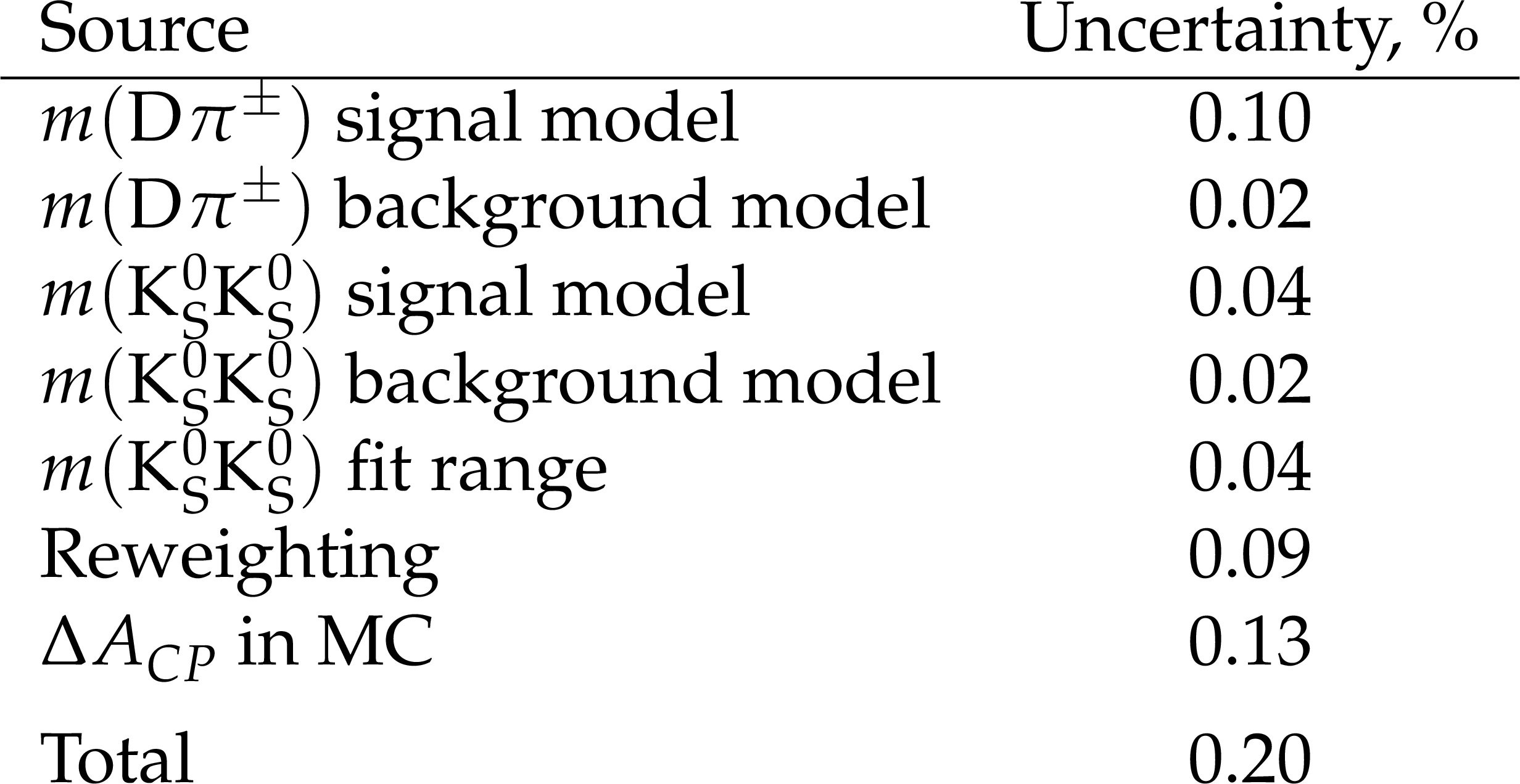
png pdf	Table 4: Absolute systematic uncertainties in the measurement of $\Delta A_{CP}$.

Summary

This is the first CMS measurement of $CP$ violation in the charm sector, paving the way for future measurements with more data, using refined techniques, and in different channels.

References
1	A. D. Sakharov	Violation of CP invariance, C asymmetry, and baryon asymmetry of the universe	Sov. Phys. Usp. 34 (1991) 392
2	N. Cabibbo	Unitary symmetry and leptonic decays	PRL 10 (1963) 531
3	M. Kobayashi and T. Maskawa	CP-violation in the renormalizable theory of weak interaction	Progress of Theoretical Physics 49 (1973) 652
4	J. H. Christenson, J. W. Cronin, V. L. Fitch, and R. Turlay	Evidence for the 2 $\pi$ decay of the $K_{2}^{0}$ meson	PRL 13 (1964) 138
5	KTeV Collaboration	Observation of direct CP violation in $K_{S, L} \to \pi \pi$ decays	PRL 83 (1999) 22	hep-ex/9905060
6	The NA48 Collaboration	A precise measurement of the direct CP violation parameter $\operatorname{Re}\left(\varepsilon^{\prime} / \varepsilon\right)$	Eur. Phys. J. C. 22 (2001) 231	hep-ex/0110019
7	BABAR Collaboration	Observation of $\mathit{CP}$ violation in the ${\mathit{B}}^{0}$ meson system	PRL 87 (2001) 091801	hep-ex/0107013
8	The Belle Collaboration	Observation of large CP-violation in the neutral B meson system	PRL 87 (2001)	hep-ex/0107061
9	BABAR Collaboration	Direct $CP$ violating asymmetry in ${B}^{0}\rightarrow{K}^{+}{\pi}^{-}$ decays	PRL 93 (2004) 131801	hep-ex/0407057
10	Belle Collaboration	Evidence for direct $CP$ violation in ${B}^{0}\rightarrow{K}^{+}{\pi}^{-}$ decays	PRL 93 (2004) 191802	hep-ex/0408100
11	LHCb Collaboration	First observation of $CP$ violation in the decays of ${B}_{s}^{0}$ mesons	PRL 110 (2013) 221601	1304.6173
12	LHCb Collaboration	Observation of CP violation in $B^{ \pm} \rightarrow D K^{ \pm}$ decays	PLB 712 (2012) 203	1203.3662
13	A. G. Cohen, D. B. Kaplan, and A. E. Nelson	Progress in electroweak baryogenesis	Annual Review of Nuclear and Particle Science 43 (1993) 27	hep-ph/9302210
14	A. Riotto and M. Trodden	Recent progress in baryogenesis	Annual Review of Nuclear and Particle Science 49 (1999) 35	hep-ph/9901362
15	W.-S. Hou	Source of CP violation for the baryon asymmetry of the Universe	Chin. J. Phys. 47 (2009) 134	0803.1234
16	S. L. Glashow, J. Iliopoulos, and L. Maiani	Weak interactions with lepton-hadron symmetry	PRD 2 (1970) 1285
17	LHCb Collaboration	Observation of CP violation in charm decays	PRL 122 (2019) 211803	1903.08726
18	A. Lenz and G. Wilkinson	Mixing and CP violation in the charm system	Ann. Rev. Nucl. Part. Sci. 71 (2021) 59	2011.04443
19	Particle Data Group Collaboration	Review of particle physics	PTEP 2022 (2022) 083C01
20	U. Nierste and S. Schacht	$CP$ violation in ${D}^{0}\rightarrow{K}_{S}{K}_{S}$	PRD 92 (2015) 054036	1508.00074
21	H.-n. Li, C.-D. Lu, and F.-S. Yu	Branching ratios and direct $CP$ asymmetries in $D \rightarrow \pi\pi$ decays	PRD 86 (2012) 036012	1203.3120
22	H.-Y. Cheng and C.-W. Chiang	Revisiting $CP$ violation in $D\rightarrow\pi\pi$ and $VP$ decays	PRD 100 (2019) 093002	1909.03063
23	F. Buccella, A. Paul, and P. Santorelli	$SU(3{)}_{F}$ breaking through final state interactions and $CP$ asymmetries in $D\rightarrow\pi\pi$ decays	PRD 99 (2019) 113001	1902.05564
24	J. Brod, A. L. Kagan, and J. Zupan	Size of direct $CP$ violation in singly Cabibbo-suppressed $D$ decays	PRD 86 (2012) 014023	1111.5000
25	LHCb Collaboration	Measurement of $CP$ asymmetry in $D^0 \to K^0_S K^0_S$ decays	PRD 104 (2021) L031102	2105.01565
26	N. Dash et al.	Search for $CP$ violation and measurement of the branching fraction in the decay $D^{0} \to K^0_S K^0_S$	PRL 119 (2017) 171801	1705.05966
27	CDF Collaboration	Measurement of CP-violation asymmetries in $D^{0} \to K^{0}_{S} \pi^+ \pi^-$	PRD 86 (2012) 032007	1207.0825
28	CMS Collaboration	HEPData record for this analysis	link
29	CMS Collaboration	Recording and reconstructing 10 billion unbiased b hadron decays in CMS	CMS Detector Performance Summary CMS-DP-2019-043, 2019 CDS
30	CMS Collaboration	Test of lepton flavor universality in B$^{\pm} \to$ K$^{\pm}\mu^+\mu^-$ and B$^{\pm} \to$ K$^{\pm}$e$^+$e$^-$ decays in proton-proton collisions at $\sqrt{s} =$ 13 TeV		CMS-BPH-22-005 2401.07090
31	CMS Tracker Group Collaboration	The CMS Phase-1 pixel detector upgrade	JINST 16 (2021) P02027	2012.14304
32	CMS Collaboration	Track impact parameter resolution for the full pseudo rapidity coverage in the 2017 dataset with the CMS Phase-1 pixel detector	CMS Detector Performance Summary CMS-DP-2020-049, 2020 CDS
33	CMS Collaboration	Performance of the CMS Level-1 trigger in proton-proton collisions at $\sqrt{s} =$ 13\,TeV	JINST 15 (2020) P10017	CMS-TRG-17-001 2006.10165
34	CMS Collaboration	The CMS trigger system	JINST 12 (2017) P01020	CMS-TRG-12-001 1609.02366
35	CMS Collaboration	The CMS experiment at the CERN LHC	JINST 3 (2008) S08004
36	T. Sjöstrand et al.	An introduction to PYTHIA 8.2	Comput. Phys. Commun. 191 (2015) 159	1410.3012
37	D. J. Lange	The EvtGen particle decay simulation package	NIM A 462 (2001) 152
38	CMS Collaboration	Extraction and validation of a new set of CMS PYTHIA8 tunes from underlying-event measurements	EPJC 80 (2020) 4	CMS-GEN-17-001 1903.12179
39	E. Barberio and Z. Was	PHOTOS --- a universal Monte Carlo for QED radiative corrections: version 2.0	Comput. Phys. Commun. 79 (1994) 291
40	GEANT4 Collaboration	GEANT 4 --- a simulation toolkit	NIM A 506 (2003) 250
41	CMS Collaboration	CMS tracking performance results from early LHC operation	EPJC 70 (2010) 1165	CMS-TRK-10-001 1007.1988
42	CMS Collaboration	Description and performance of track and primary-vertex reconstruction with the CMS tracker	JINST 9 (2014) P10009	CMS-TRK-11-001 1405.6569
43	N. L. Johnson	Systems of frequency curves generated by methods of translation	Biometrika 36 (1949) 149
44	M. J. Oreglia	A study of the reactions $\psi^\prime \to \gamma \gamma \psi$	PhD thesis, Stanford University, SLAC Report SLAC-R-236, 1980 link
45	CLEO Collaboration	Search for CP violation in $D^0 \to K^0_S \pi^{+}\pi^{-}$	PRD 70 (2004) 091101	hep-ex/0311033

Compact Muon Solenoid LHC, CERN

© Copyright CERN 2024 for the benefit of the CMS Collaboration