Processing math: 100%

Compact Muon Solenoid
LHC, CERN

Visit us: CMS Public Website, CMS Physics ; Contact us: CMS Publications Committee

CMS-PAS-BPH-22-005

Test of lepton flavor universality in $\mathrm{B}^{\pm}\rightarrow \mathrm{K}^\pm \ell^+ \ell^-$ decays

CMS Collaboration

31 August 2023

Abstract: A test of lepton flavor universality in $\mathrm{B}^\pm \to \mathrm{K}^\pm\ell^+\ell^-$ decays, where $\ell$ is a muon or electron, as well as a measurement of differential and inclusive branching fractions of a nonresonant $\mathrm{B}^\pm \to\mathrm{K}^\pm\mu^+\mu^-$ decay with the CMS experiment at the LHC are presented. The analysis is made possible by a dedicated data set of proton-proton collisions at $\sqrt{s} =$ 13 TeV recorded in 2018, using a special high-rate data stream designed for collecting about 10 billion unbiased b hadron decays. The ratio of the branching fractions ${\cal B}(\mathrm{B}^\pm \to \mathrm{K}^\pm\mu^+\mu^-$) to ${\cal B}(\mathrm{B}^\pm \to \mathrm{K}^\pm\mathrm{e^+e^-}$) is measured as a double ratio $R(\mathrm{K})$ of these decays to the respective branching fractions of the $\mathrm{B}^\pm \to \mathrm{J}/\psi\mathrm{K}^\pm$ ($\mathrm{J}/\psi \to \mu^+\mu^-)$ and ($\mathrm{J}/\psi\to \mathrm{e^+e^-})$ decays, which allow for significant cancellation of systematic uncertainties. The ratio $R(\mathrm{K})$ is measured in a range 1.1 $< q^2 <$ 6.0 GeV$^2$, where $q$ is the invariant mass of the lepton pair, and is found to be $R({\rm K})=$ 0.78 $^{+0.47}_{-0.23}$, in agreement with the standard model expectation within one standard deviation. This measurement is limited by the statistical precision of the electron channel. The inclusive branching fraction in the same $q^2$ range of ${\cal B}(\mathrm{B}^\pm \to \mathrm{K}^\pm\mu^+\mu^-) =$ ( 12.42 $\pm$ 0.68 ) $\times$ 10$^{-8}$ is consistent with and has a comparable precision to the present world average value.

Links: CDS record (PDF) ; CADI line (restricted) ; These preliminary results are superseded in this paper, Submitted to ROPP. The superseded preliminary plots can be found here.

Figures
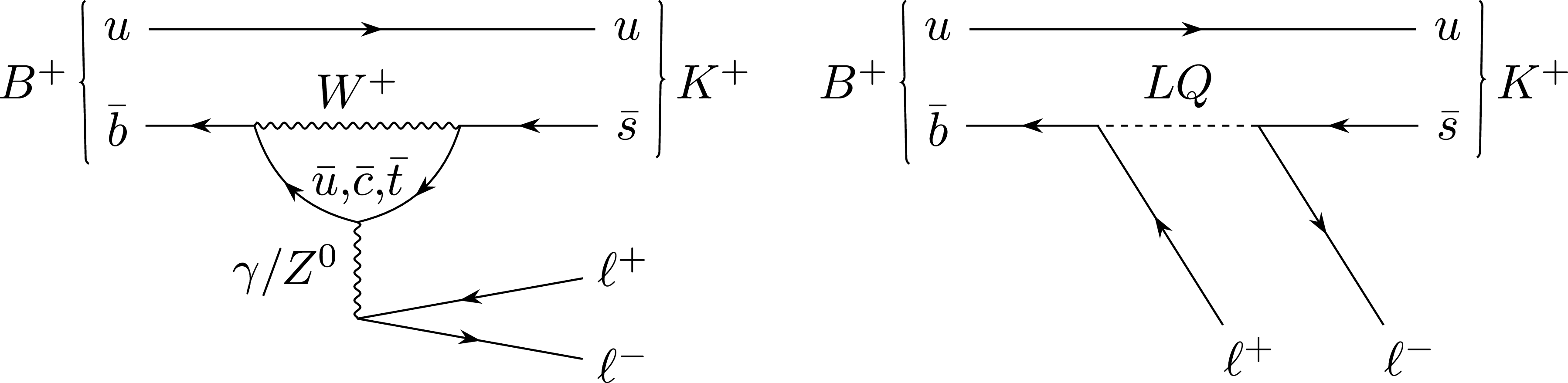
png pdf	Figure 1: Representative Feynman diagrams for the decay of a ${\mathrm{B}^{+}}$ meson into a $\mathrm{K^+}$ meson and a lepton pair for the SM (left) and for a BSM scenario introducing a leptoquark (LQ) with flavor-dependent couplings (right).
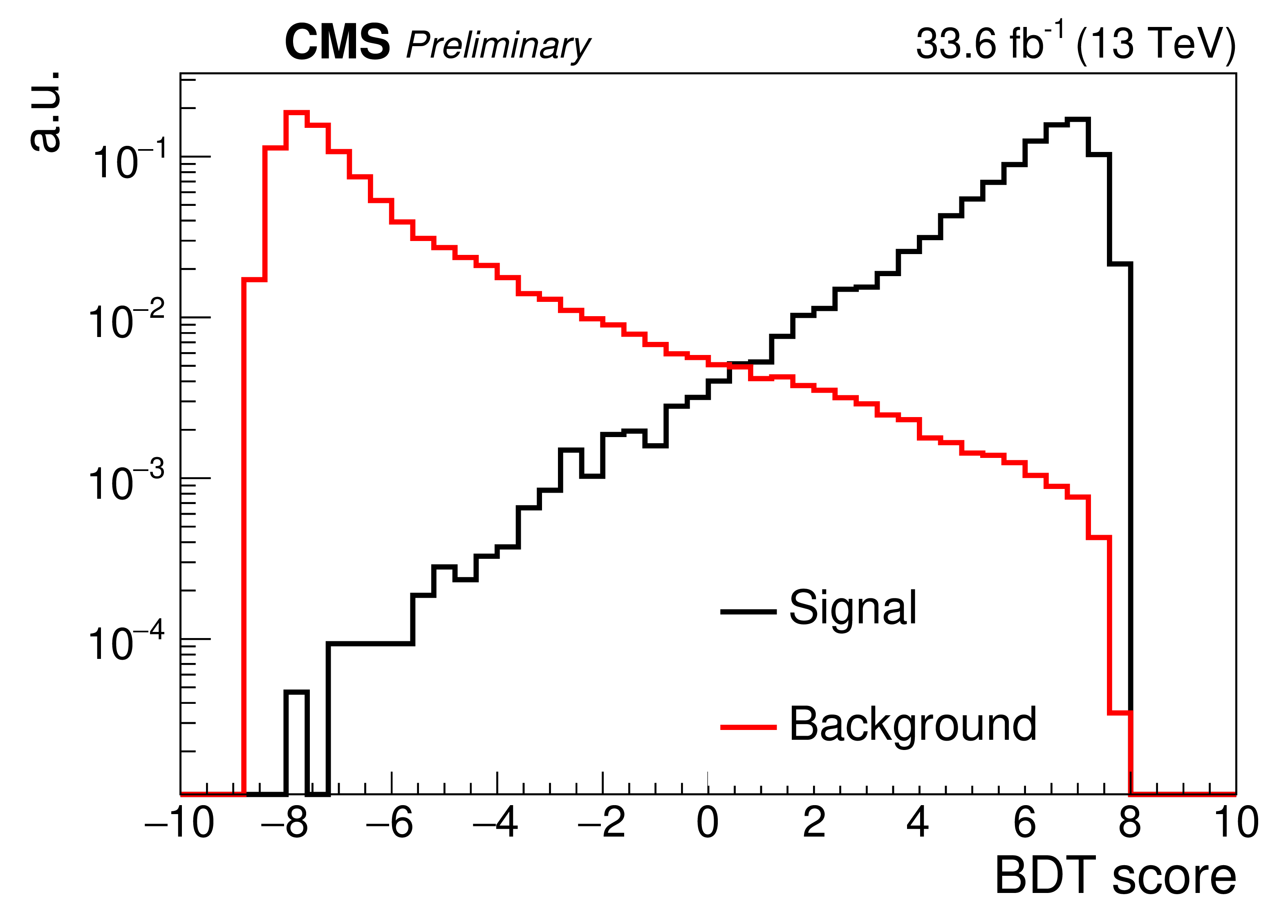
png pdf	Figure 2: Analysis BDT score for signal (MC simulation in red) and background (same-sign dimuon data in black) for the muon channel.
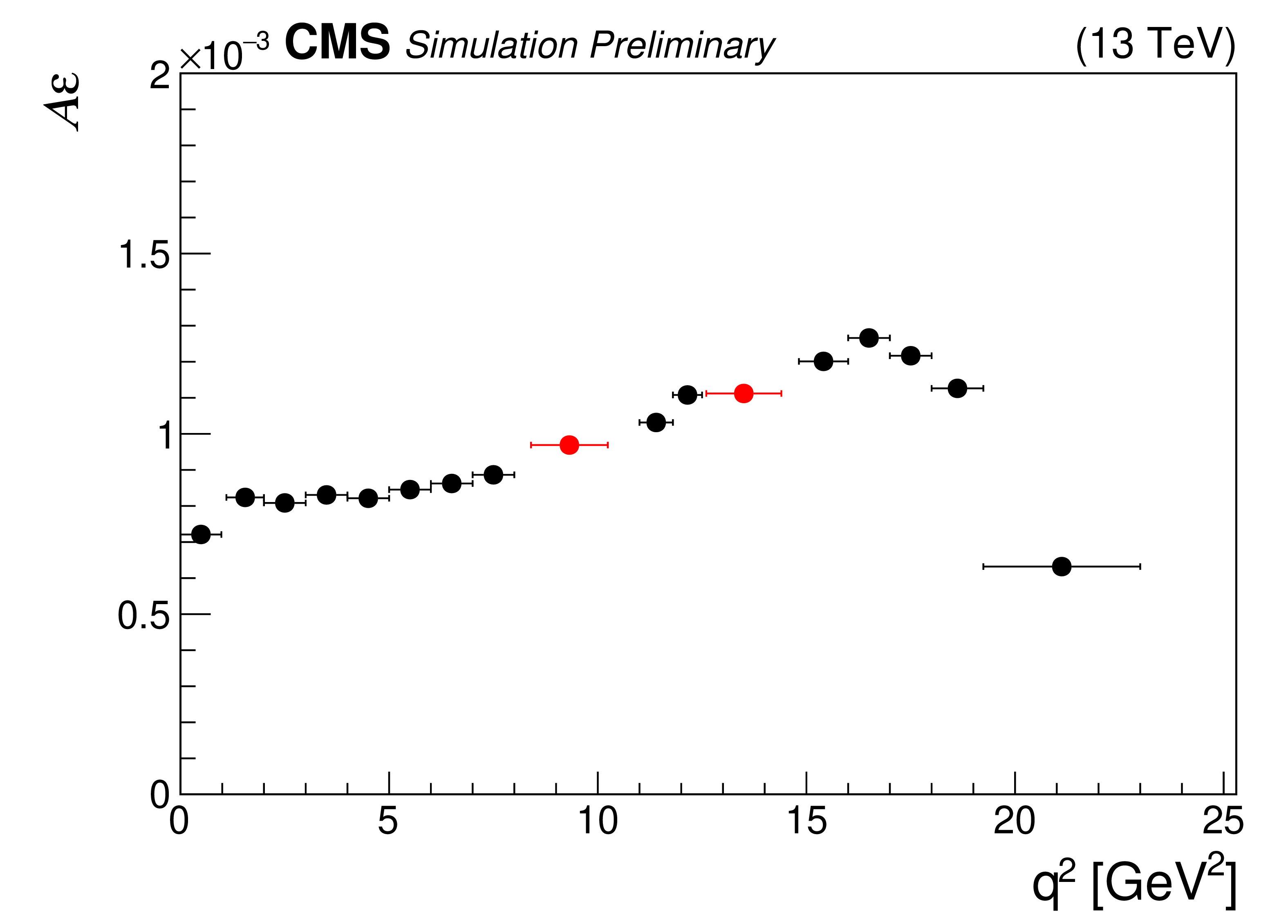
png pdf	Figure 3: The product of acceptance and efficiency (${\cal A}\epsilon$) as a function of the muon pair $q^2$, as measured in simulated signal events, corrected to match data. Regions corresponding to resonances are displayed with red markers.
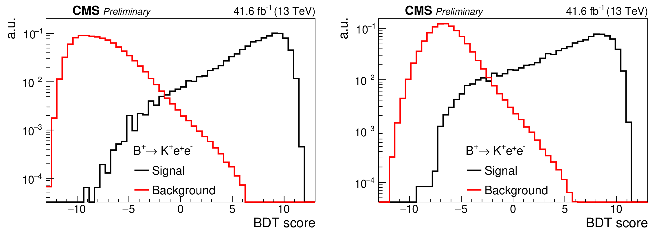
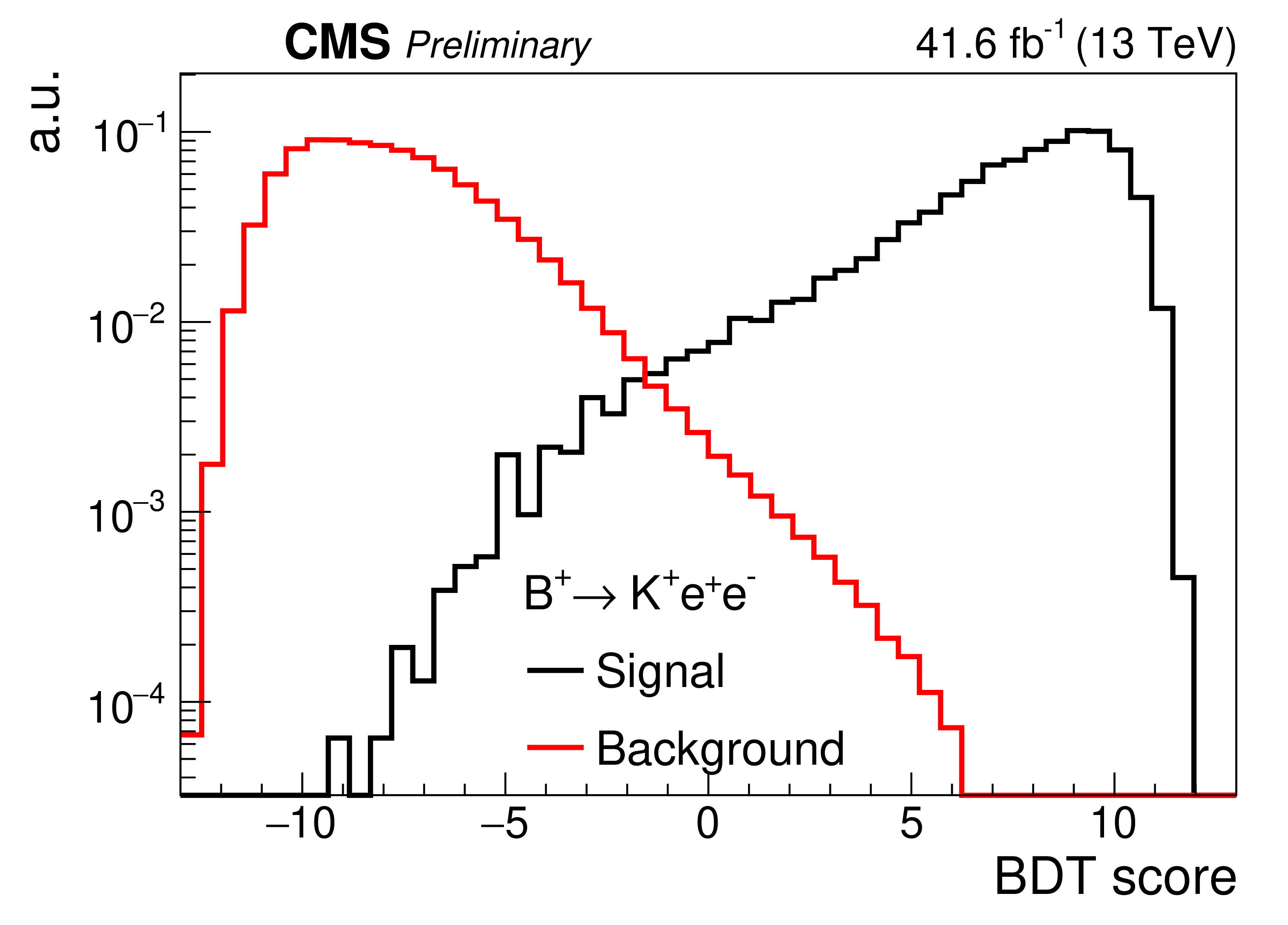
png pdf	Figure 4: Analysis BDT score for signal (MC simulation in red) and background (same-sign dielectron data in black) for the electron channel for PF-PF (left) and PF-LP (right) categories.
png pdf	Figure 4-a: Analysis BDT score for signal (MC simulation in red) and background (same-sign dielectron data in black) for the electron channel for PF-PF (left) and PF-LP (right) categories.
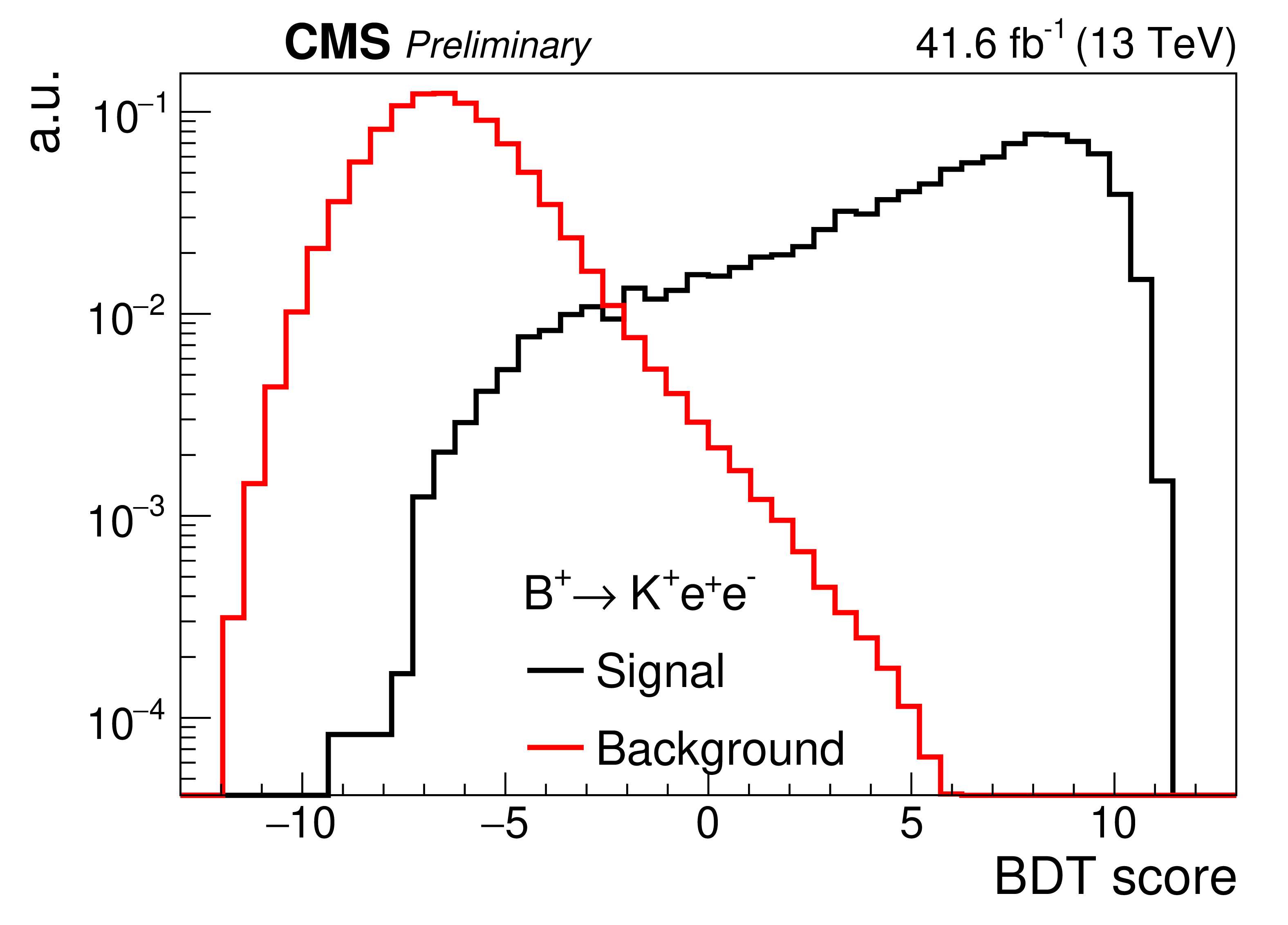
png pdf	Figure 4-b: Analysis BDT score for signal (MC simulation in red) and background (same-sign dielectron data in black) for the electron channel for PF-PF (left) and PF-LP (right) categories.
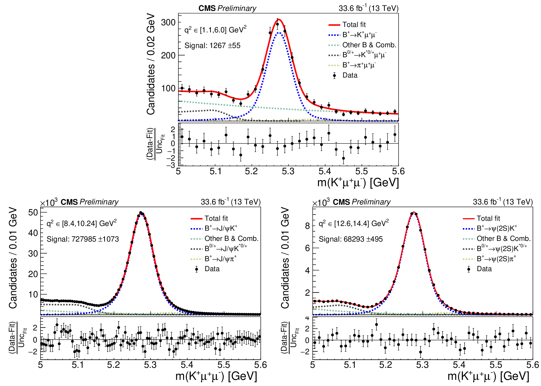
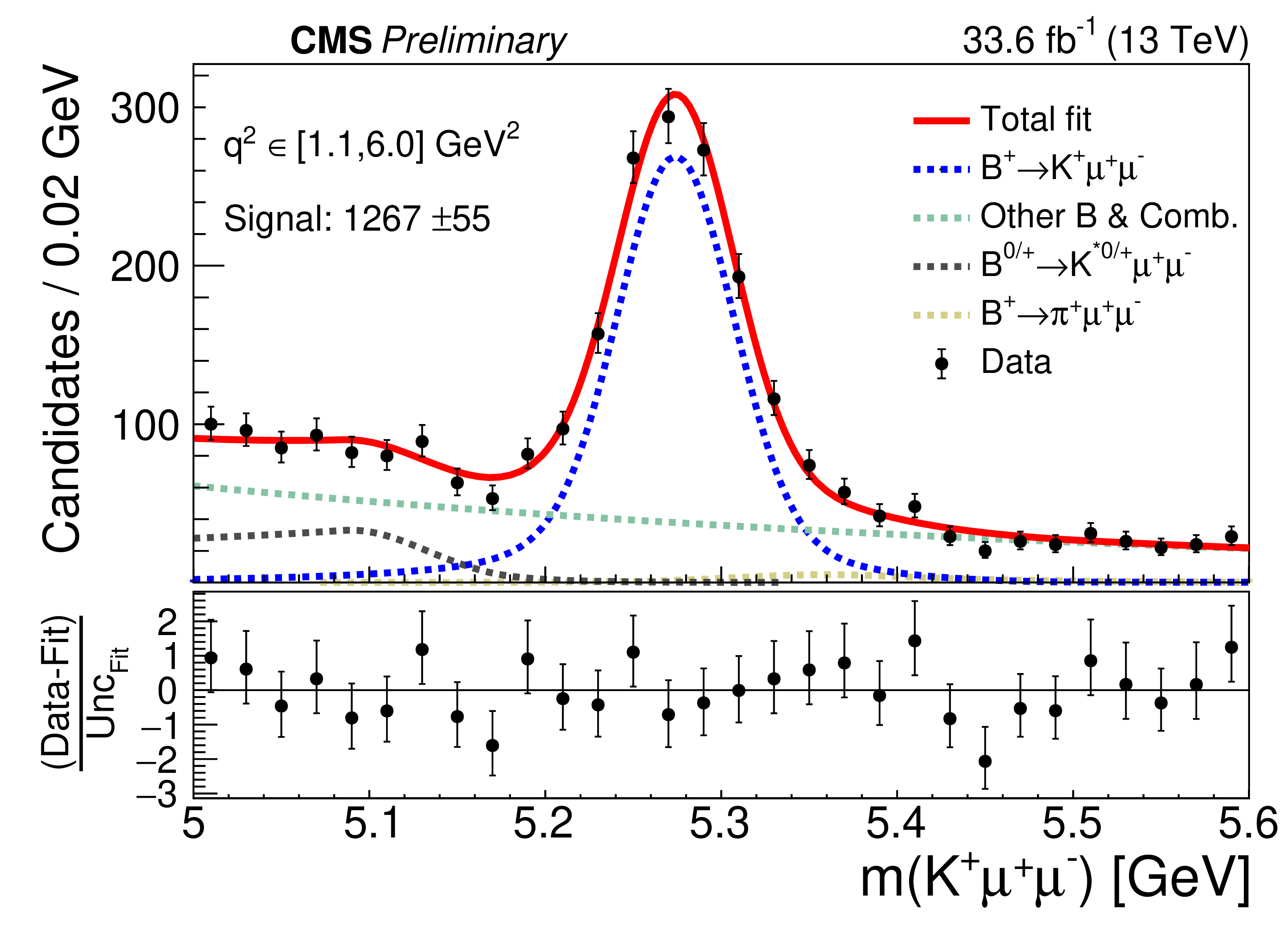
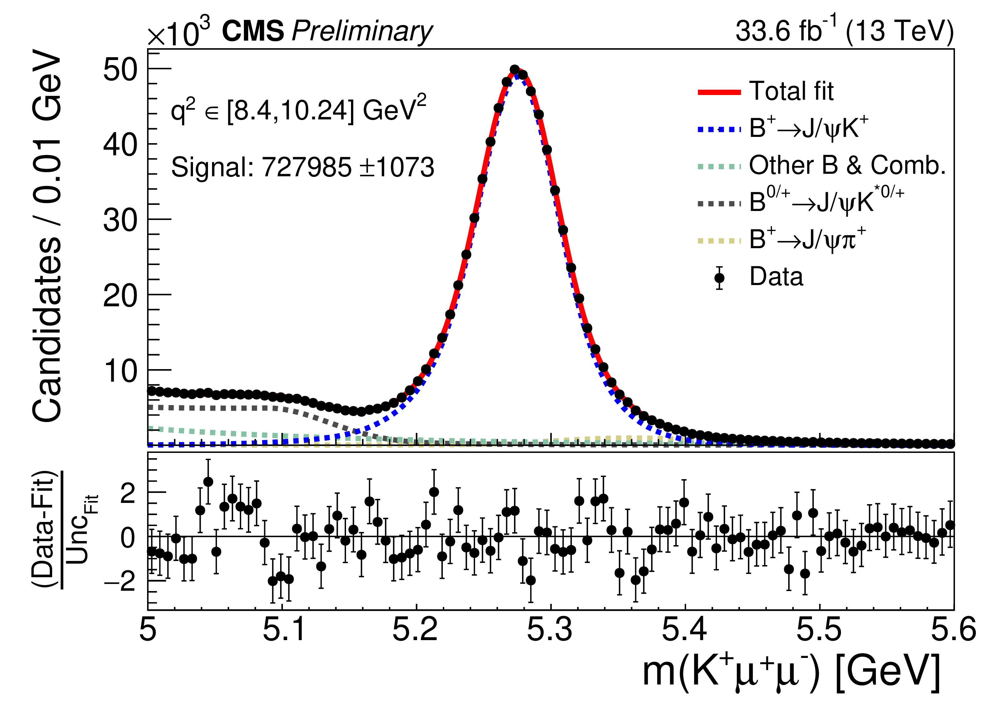
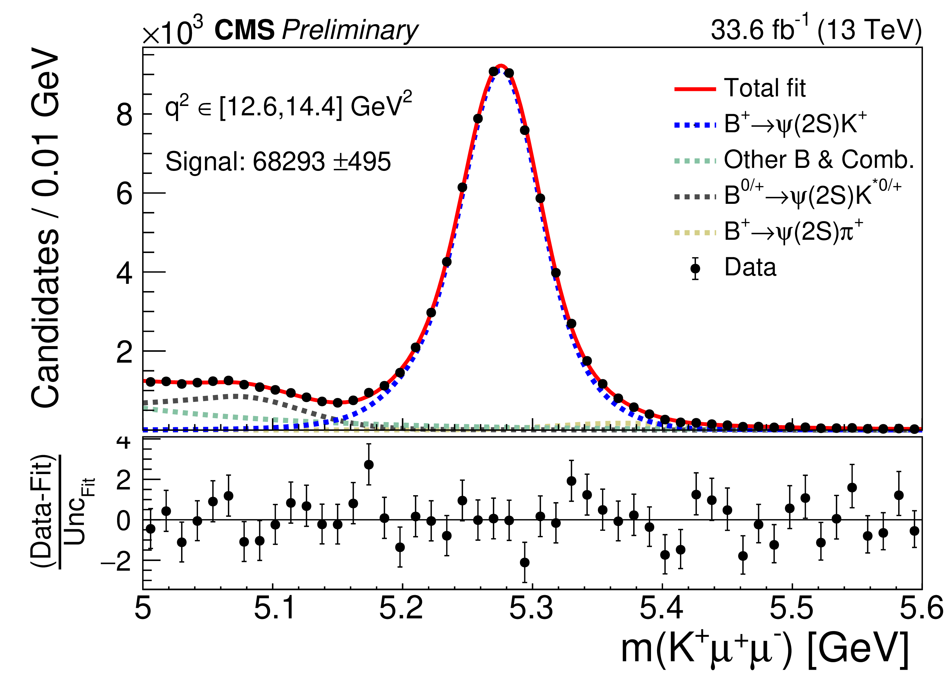
png pdf	Figure 5: Results of unbinned likelihood fits to the invariant mass distributions in the (upper row) low-$q^2$ signal region and in the (lower row) ${\mathrm{B}^{+}} \to {\mathrm{J}/\psi} (\mu^{+}\mu^{-})\mathrm{K^+}$ (left) and ${\mathrm{B}^{+}} \to \psi(2\mathrm{S})(\mu^{+}\mu^{-})\mathrm{K^+}$ (right) control regions. The lower panels show the distribution of the pull, which is defined as the difference between the data and the fit, divided by the fit uncertainty.
png pdf	Figure 5-a: Results of unbinned likelihood fits to the invariant mass distributions in the (upper row) low-$q^2$ signal region and in the (lower row) ${\mathrm{B}^{+}} \to {\mathrm{J}/\psi} (\mu^{+}\mu^{-})\mathrm{K^+}$ (left) and ${\mathrm{B}^{+}} \to \psi(2\mathrm{S})(\mu^{+}\mu^{-})\mathrm{K^+}$ (right) control regions. The lower panels show the distribution of the pull, which is defined as the difference between the data and the fit, divided by the fit uncertainty.
png pdf	Figure 5-b: Results of unbinned likelihood fits to the invariant mass distributions in the (upper row) low-$q^2$ signal region and in the (lower row) ${\mathrm{B}^{+}} \to {\mathrm{J}/\psi} (\mu^{+}\mu^{-})\mathrm{K^+}$ (left) and ${\mathrm{B}^{+}} \to \psi(2\mathrm{S})(\mu^{+}\mu^{-})\mathrm{K^+}$ (right) control regions. The lower panels show the distribution of the pull, which is defined as the difference between the data and the fit, divided by the fit uncertainty.
png pdf	Figure 5-c: Results of unbinned likelihood fits to the invariant mass distributions in the (upper row) low-$q^2$ signal region and in the (lower row) ${\mathrm{B}^{+}} \to {\mathrm{J}/\psi} (\mu^{+}\mu^{-})\mathrm{K^+}$ (left) and ${\mathrm{B}^{+}} \to \psi(2\mathrm{S})(\mu^{+}\mu^{-})\mathrm{K^+}$ (right) control regions. The lower panels show the distribution of the pull, which is defined as the difference between the data and the fit, divided by the fit uncertainty.
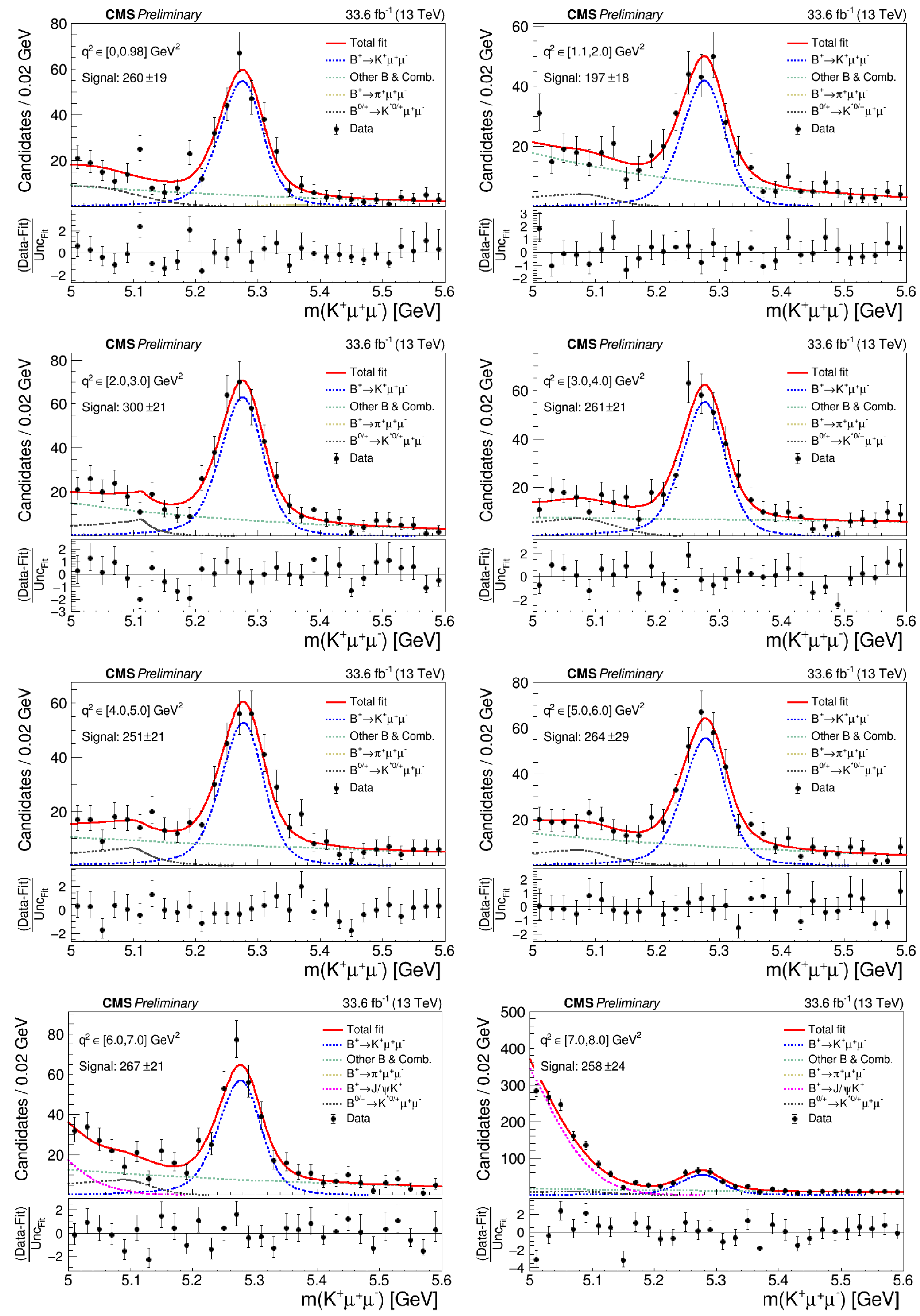
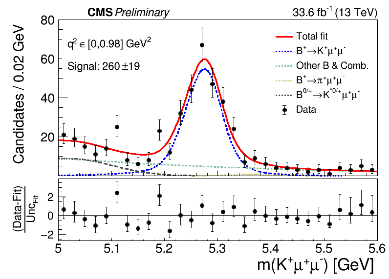
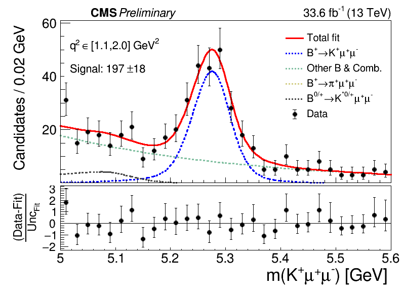
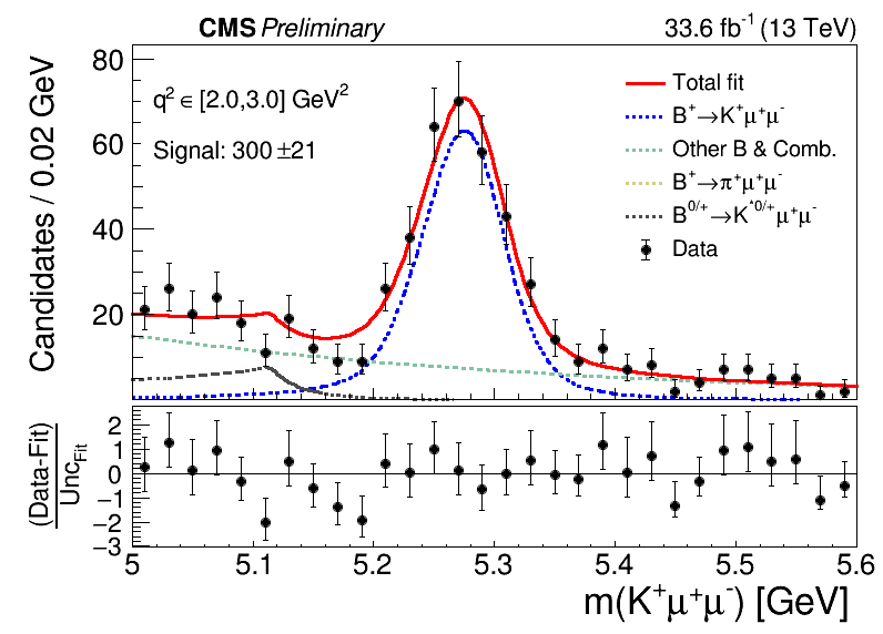
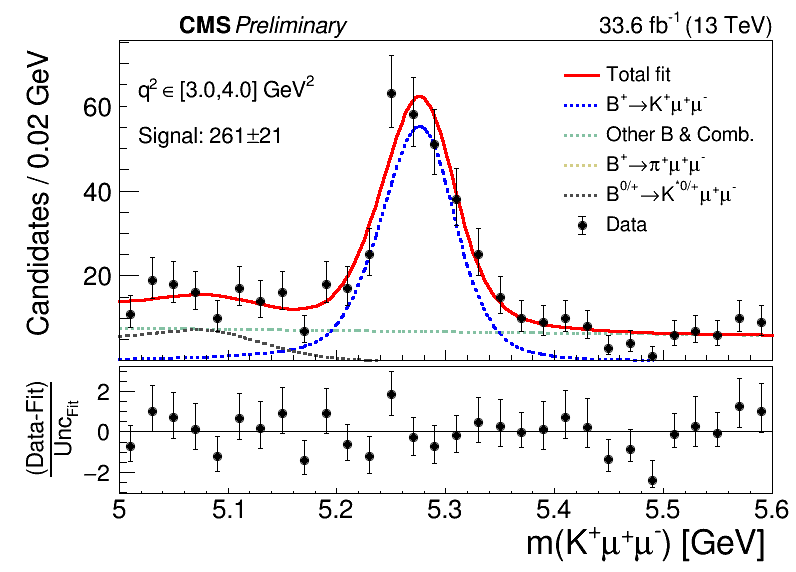
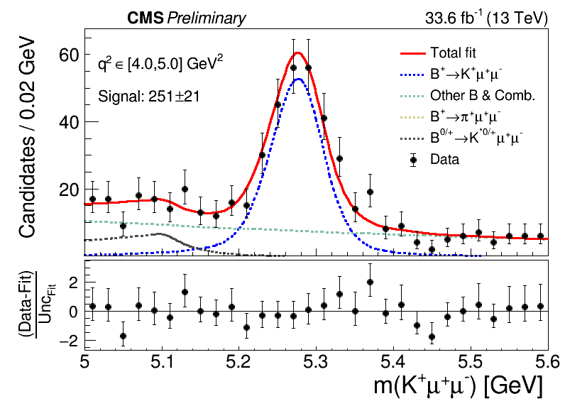
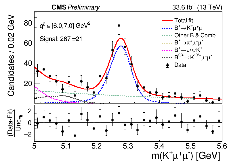
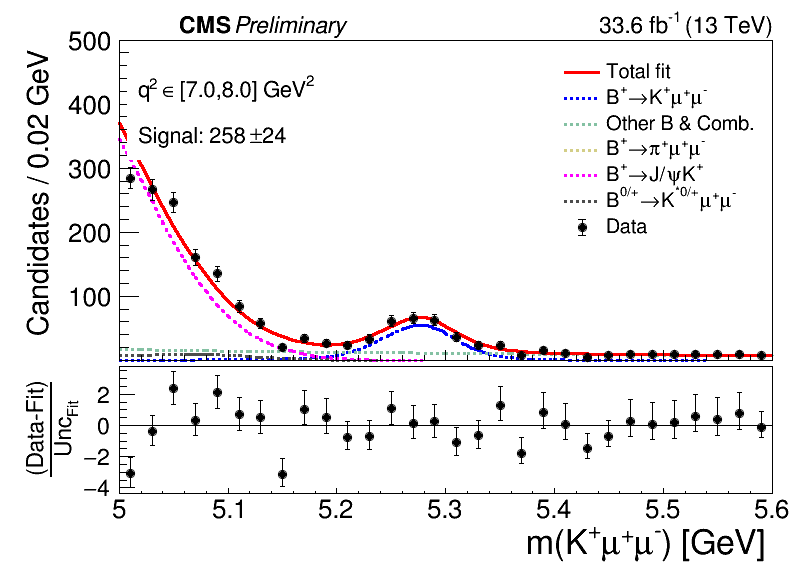
png pdf	Figure 6: The $\mathrm{K^+} \mu^{+} \mu^{-}$ invariant mass distributions in various $q^2$ bins, with the result of the simultaneous fit overlaid in blue and the individual fit components as described in the legends for (from upper left to lower right): $[0,0.98]$, $[1.1,2.0]$, $[2.0,3.0] [3.0,4.0]$, $[4.0,5.0]$, $[5.0,6.0]$, $[6.0,7.0]$, and $[7.0,8.0]$, $q^2$ bins. The lower panels show the distribution of the pull, which is defined as the difference between the data and the fit, divided by the fit uncertainty.
png	Figure 6-a: The $\mathrm{K^+} \mu^{+} \mu^{-}$ invariant mass distributions in various $q^2$ bins, with the result of the simultaneous fit overlaid in blue and the individual fit components as described in the legends for (from upper left to lower right): $[0,0.98]$, $[1.1,2.0]$, $[2.0,3.0] [3.0,4.0]$, $[4.0,5.0]$, $[5.0,6.0]$, $[6.0,7.0]$, and $[7.0,8.0]$, $q^2$ bins. The lower panels show the distribution of the pull, which is defined as the difference between the data and the fit, divided by the fit uncertainty.
png	Figure 6-b: The $\mathrm{K^+} \mu^{+} \mu^{-}$ invariant mass distributions in various $q^2$ bins, with the result of the simultaneous fit overlaid in blue and the individual fit components as described in the legends for (from upper left to lower right): $[0,0.98]$, $[1.1,2.0]$, $[2.0,3.0] [3.0,4.0]$, $[4.0,5.0]$, $[5.0,6.0]$, $[6.0,7.0]$, and $[7.0,8.0]$, $q^2$ bins. The lower panels show the distribution of the pull, which is defined as the difference between the data and the fit, divided by the fit uncertainty.
png	Figure 6-c: The $\mathrm{K^+} \mu^{+} \mu^{-}$ invariant mass distributions in various $q^2$ bins, with the result of the simultaneous fit overlaid in blue and the individual fit components as described in the legends for (from upper left to lower right): $[0,0.98]$, $[1.1,2.0]$, $[2.0,3.0] [3.0,4.0]$, $[4.0,5.0]$, $[5.0,6.0]$, $[6.0,7.0]$, and $[7.0,8.0]$, $q^2$ bins. The lower panels show the distribution of the pull, which is defined as the difference between the data and the fit, divided by the fit uncertainty.
png	Figure 6-d: The $\mathrm{K^+} \mu^{+} \mu^{-}$ invariant mass distributions in various $q^2$ bins, with the result of the simultaneous fit overlaid in blue and the individual fit components as described in the legends for (from upper left to lower right): $[0,0.98]$, $[1.1,2.0]$, $[2.0,3.0] [3.0,4.0]$, $[4.0,5.0]$, $[5.0,6.0]$, $[6.0,7.0]$, and $[7.0,8.0]$, $q^2$ bins. The lower panels show the distribution of the pull, which is defined as the difference between the data and the fit, divided by the fit uncertainty.
png	Figure 6-e: The $\mathrm{K^+} \mu^{+} \mu^{-}$ invariant mass distributions in various $q^2$ bins, with the result of the simultaneous fit overlaid in blue and the individual fit components as described in the legends for (from upper left to lower right): $[0,0.98]$, $[1.1,2.0]$, $[2.0,3.0] [3.0,4.0]$, $[4.0,5.0]$, $[5.0,6.0]$, $[6.0,7.0]$, and $[7.0,8.0]$, $q^2$ bins. The lower panels show the distribution of the pull, which is defined as the difference between the data and the fit, divided by the fit uncertainty.
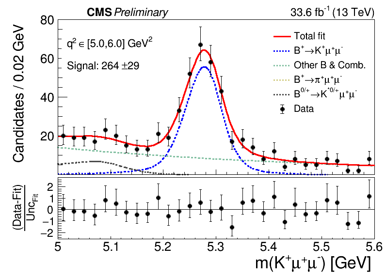
png	Figure 6-f: The $\mathrm{K^+} \mu^{+} \mu^{-}$ invariant mass distributions in various $q^2$ bins, with the result of the simultaneous fit overlaid in blue and the individual fit components as described in the legends for (from upper left to lower right): $[0,0.98]$, $[1.1,2.0]$, $[2.0,3.0] [3.0,4.0]$, $[4.0,5.0]$, $[5.0,6.0]$, $[6.0,7.0]$, and $[7.0,8.0]$, $q^2$ bins. The lower panels show the distribution of the pull, which is defined as the difference between the data and the fit, divided by the fit uncertainty.
png	Figure 6-g: The $\mathrm{K^+} \mu^{+} \mu^{-}$ invariant mass distributions in various $q^2$ bins, with the result of the simultaneous fit overlaid in blue and the individual fit components as described in the legends for (from upper left to lower right): $[0,0.98]$, $[1.1,2.0]$, $[2.0,3.0] [3.0,4.0]$, $[4.0,5.0]$, $[5.0,6.0]$, $[6.0,7.0]$, and $[7.0,8.0]$, $q^2$ bins. The lower panels show the distribution of the pull, which is defined as the difference between the data and the fit, divided by the fit uncertainty.
png	Figure 6-h: The $\mathrm{K^+} \mu^{+} \mu^{-}$ invariant mass distributions in various $q^2$ bins, with the result of the simultaneous fit overlaid in blue and the individual fit components as described in the legends for (from upper left to lower right): $[0,0.98]$, $[1.1,2.0]$, $[2.0,3.0] [3.0,4.0]$, $[4.0,5.0]$, $[5.0,6.0]$, $[6.0,7.0]$, and $[7.0,8.0]$, $q^2$ bins. The lower panels show the distribution of the pull, which is defined as the difference between the data and the fit, divided by the fit uncertainty.
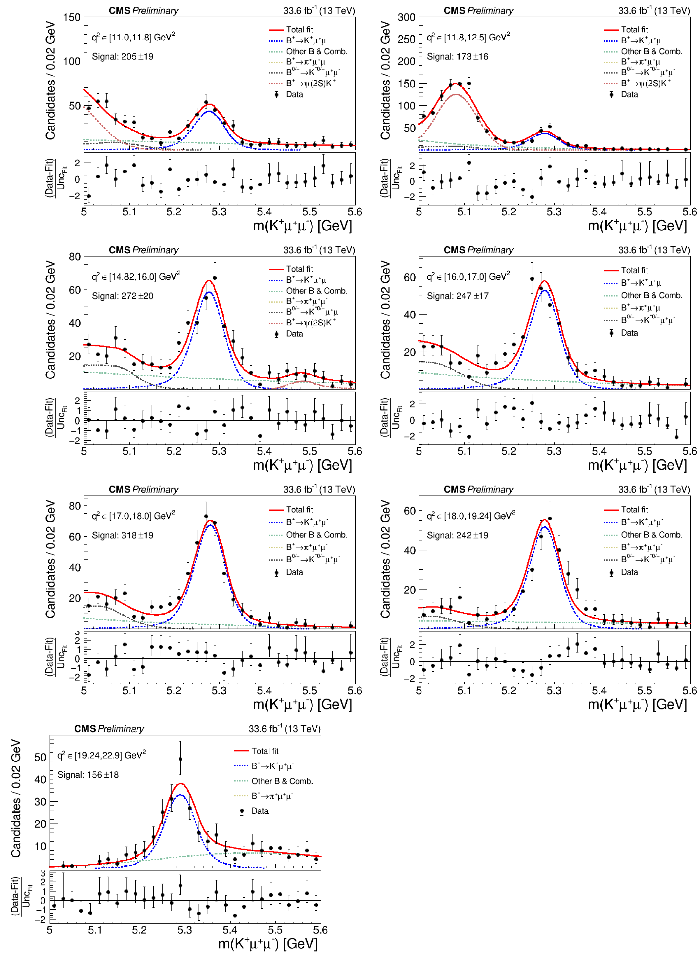
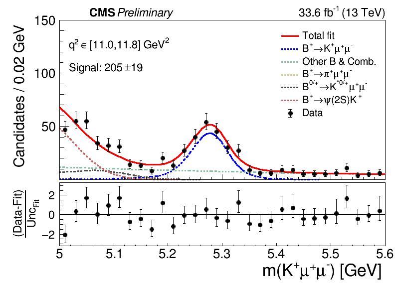
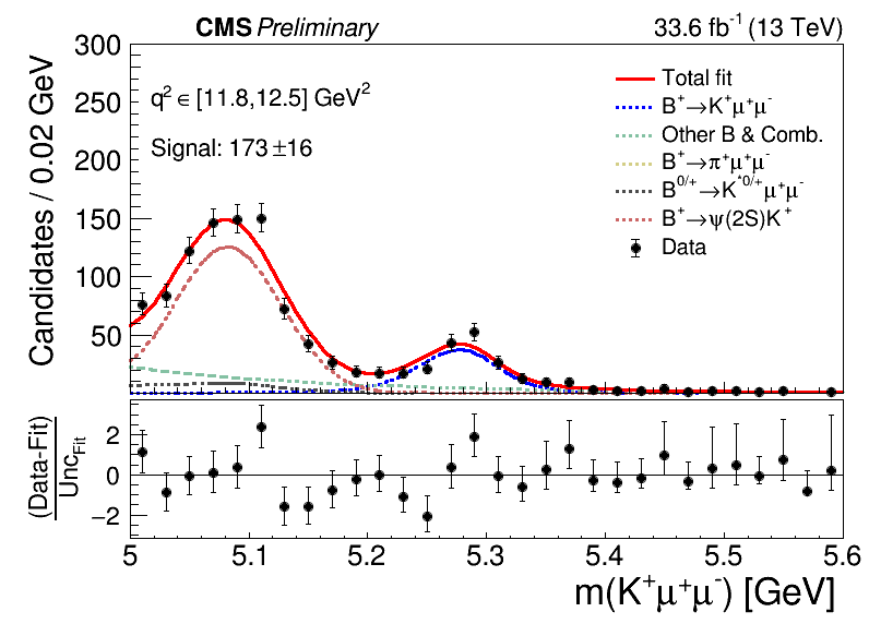
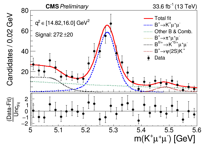
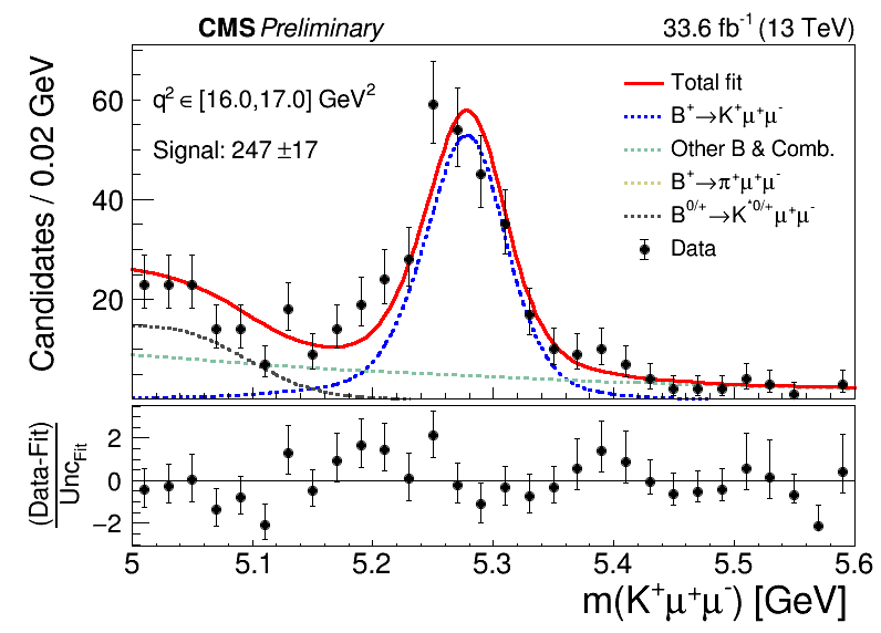
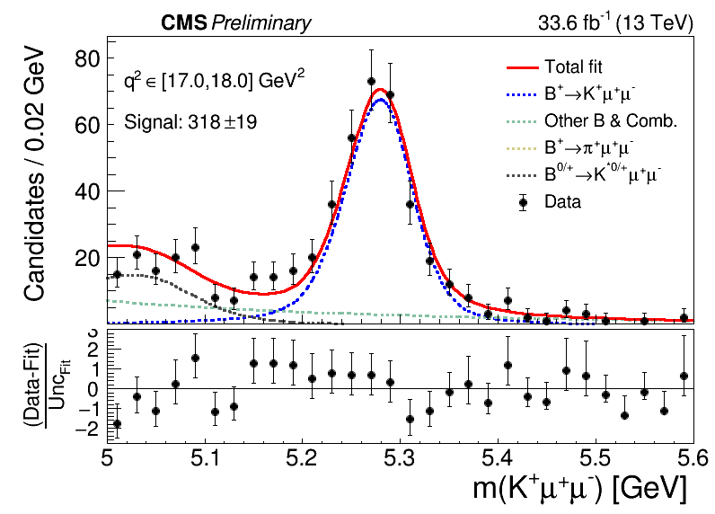
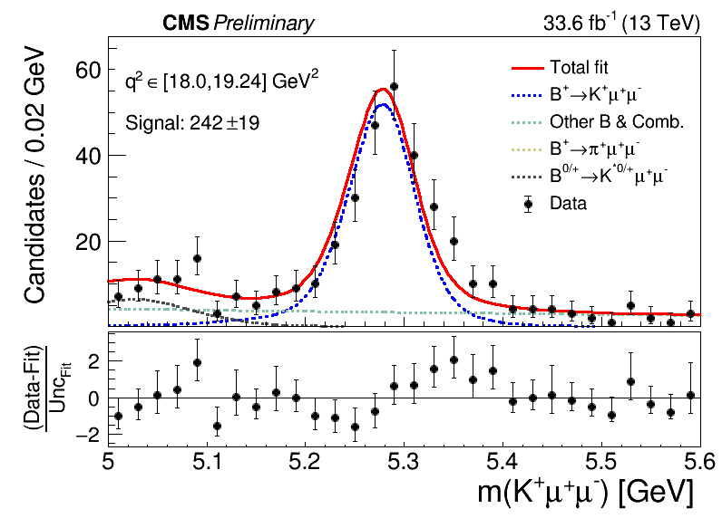
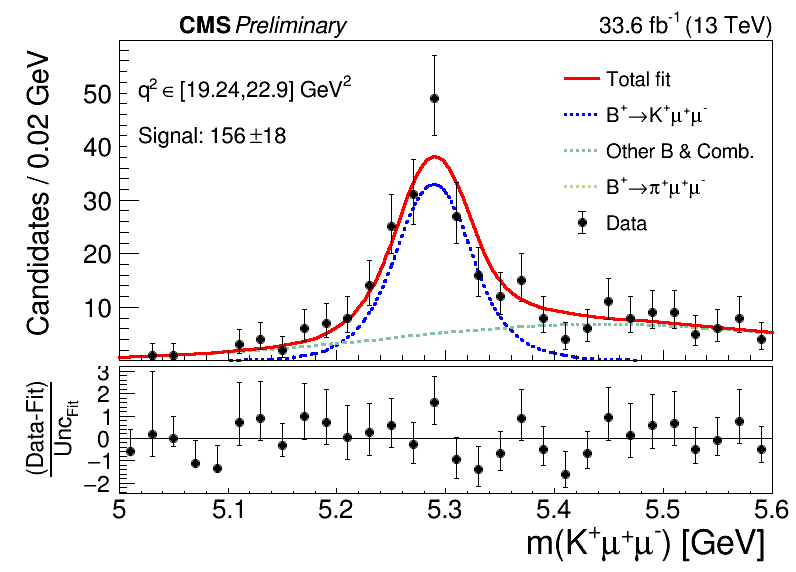
png pdf	Figure 7: The $\mathrm{K^+} \mu^{+} \mu^{-}$ invariant mass distributions in various $q^2$ bins, with the result of the simultaneous fit overlaid in blue and the individual fit components as described in the legends for (from upper left to lower right): $[11.0,11.8]$, $[11.8,12.5]$, $[14.82,16.0]$, $[16.0,17.0]$, $[17.0,18.0]$, $[18.0,19.24]$, and $[19.24,22.9]$ GeV$^2$ $q^2$ bins. The lower panels show the distribution of the pull, which is defined as the difference between the data and the fit, divided by the fit uncertainty.
png	Figure 7-a: The $\mathrm{K^+} \mu^{+} \mu^{-}$ invariant mass distributions in various $q^2$ bins, with the result of the simultaneous fit overlaid in blue and the individual fit components as described in the legends for (from upper left to lower right): $[11.0,11.8]$, $[11.8,12.5]$, $[14.82,16.0]$, $[16.0,17.0]$, $[17.0,18.0]$, $[18.0,19.24]$, and $[19.24,22.9]$ GeV$^2$ $q^2$ bins. The lower panels show the distribution of the pull, which is defined as the difference between the data and the fit, divided by the fit uncertainty.
png	Figure 7-b: The $\mathrm{K^+} \mu^{+} \mu^{-}$ invariant mass distributions in various $q^2$ bins, with the result of the simultaneous fit overlaid in blue and the individual fit components as described in the legends for (from upper left to lower right): $[11.0,11.8]$, $[11.8,12.5]$, $[14.82,16.0]$, $[16.0,17.0]$, $[17.0,18.0]$, $[18.0,19.24]$, and $[19.24,22.9]$ GeV$^2$ $q^2$ bins. The lower panels show the distribution of the pull, which is defined as the difference between the data and the fit, divided by the fit uncertainty.
png	Figure 7-c: The $\mathrm{K^+} \mu^{+} \mu^{-}$ invariant mass distributions in various $q^2$ bins, with the result of the simultaneous fit overlaid in blue and the individual fit components as described in the legends for (from upper left to lower right): $[11.0,11.8]$, $[11.8,12.5]$, $[14.82,16.0]$, $[16.0,17.0]$, $[17.0,18.0]$, $[18.0,19.24]$, and $[19.24,22.9]$ GeV$^2$ $q^2$ bins. The lower panels show the distribution of the pull, which is defined as the difference between the data and the fit, divided by the fit uncertainty.
png	Figure 7-d: The $\mathrm{K^+} \mu^{+} \mu^{-}$ invariant mass distributions in various $q^2$ bins, with the result of the simultaneous fit overlaid in blue and the individual fit components as described in the legends for (from upper left to lower right): $[11.0,11.8]$, $[11.8,12.5]$, $[14.82,16.0]$, $[16.0,17.0]$, $[17.0,18.0]$, $[18.0,19.24]$, and $[19.24,22.9]$ GeV$^2$ $q^2$ bins. The lower panels show the distribution of the pull, which is defined as the difference between the data and the fit, divided by the fit uncertainty.
png	Figure 7-e: The $\mathrm{K^+} \mu^{+} \mu^{-}$ invariant mass distributions in various $q^2$ bins, with the result of the simultaneous fit overlaid in blue and the individual fit components as described in the legends for (from upper left to lower right): $[11.0,11.8]$, $[11.8,12.5]$, $[14.82,16.0]$, $[16.0,17.0]$, $[17.0,18.0]$, $[18.0,19.24]$, and $[19.24,22.9]$ GeV$^2$ $q^2$ bins. The lower panels show the distribution of the pull, which is defined as the difference between the data and the fit, divided by the fit uncertainty.
png	Figure 7-f: The $\mathrm{K^+} \mu^{+} \mu^{-}$ invariant mass distributions in various $q^2$ bins, with the result of the simultaneous fit overlaid in blue and the individual fit components as described in the legends for (from upper left to lower right): $[11.0,11.8]$, $[11.8,12.5]$, $[14.82,16.0]$, $[16.0,17.0]$, $[17.0,18.0]$, $[18.0,19.24]$, and $[19.24,22.9]$ GeV$^2$ $q^2$ bins. The lower panels show the distribution of the pull, which is defined as the difference between the data and the fit, divided by the fit uncertainty.
png	Figure 7-g: The $\mathrm{K^+} \mu^{+} \mu^{-}$ invariant mass distributions in various $q^2$ bins, with the result of the simultaneous fit overlaid in blue and the individual fit components as described in the legends for (from upper left to lower right): $[11.0,11.8]$, $[11.8,12.5]$, $[14.82,16.0]$, $[16.0,17.0]$, $[17.0,18.0]$, $[18.0,19.24]$, and $[19.24,22.9]$ GeV$^2$ $q^2$ bins. The lower panels show the distribution of the pull, which is defined as the difference between the data and the fit, divided by the fit uncertainty.
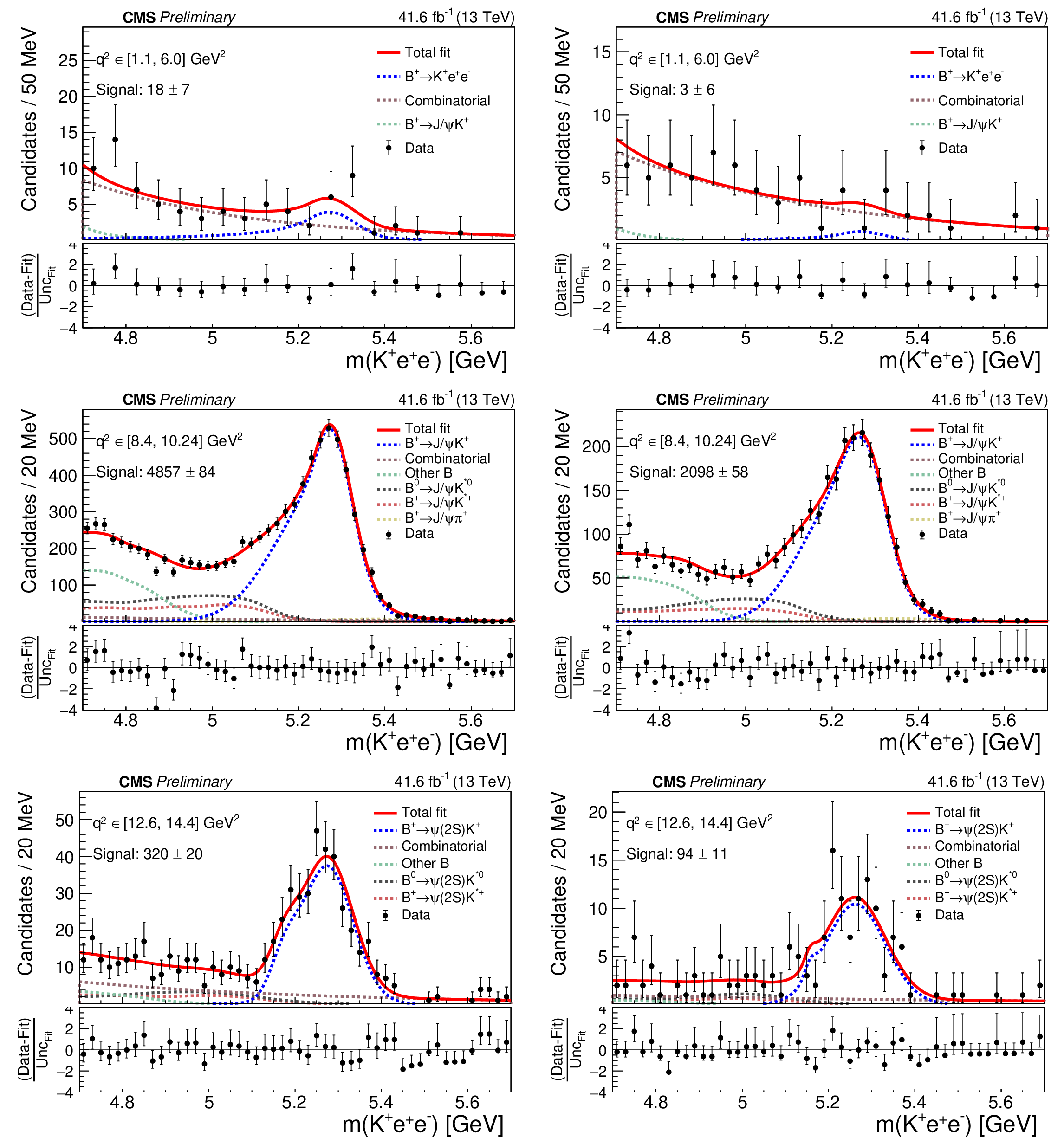
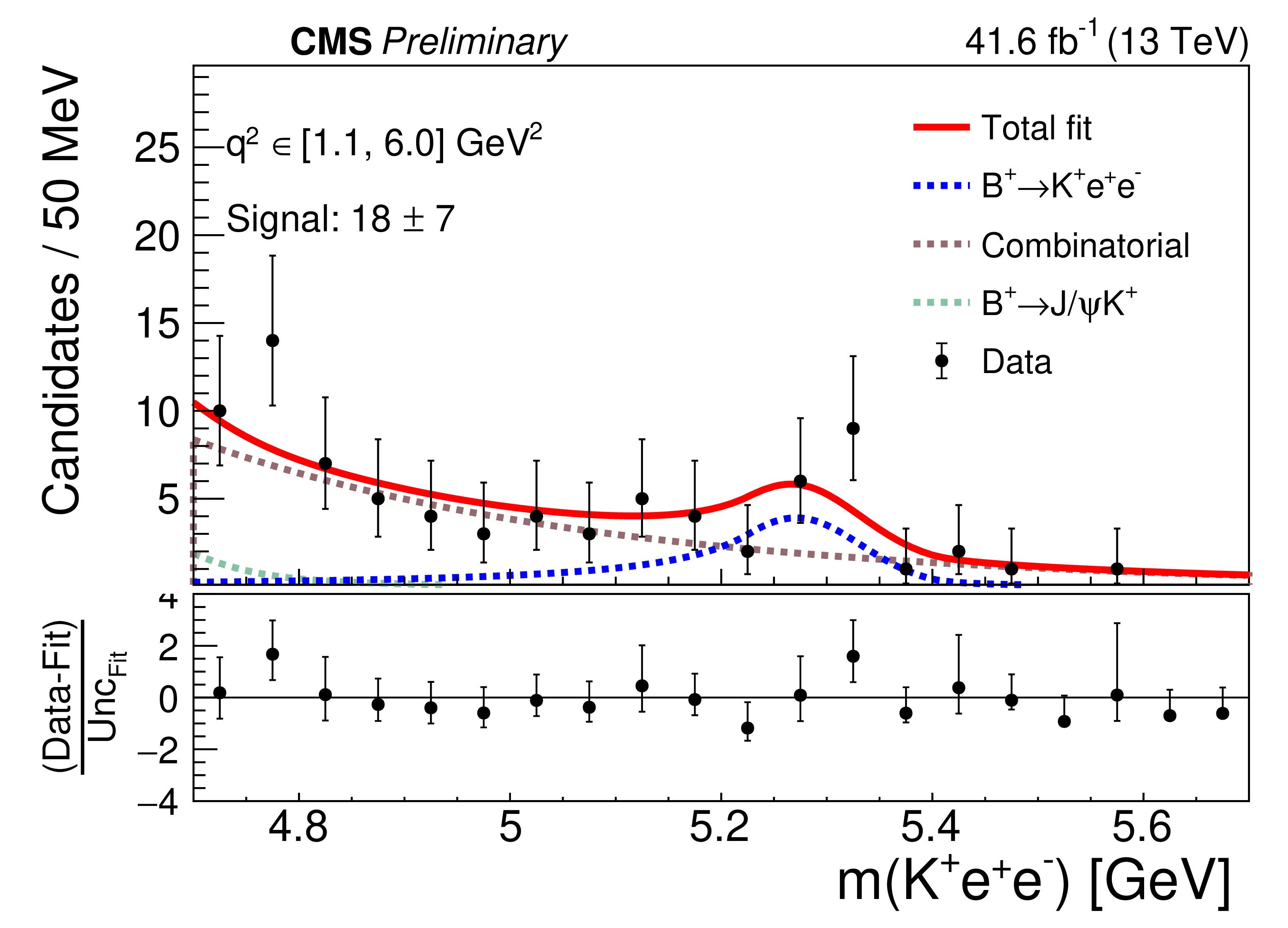
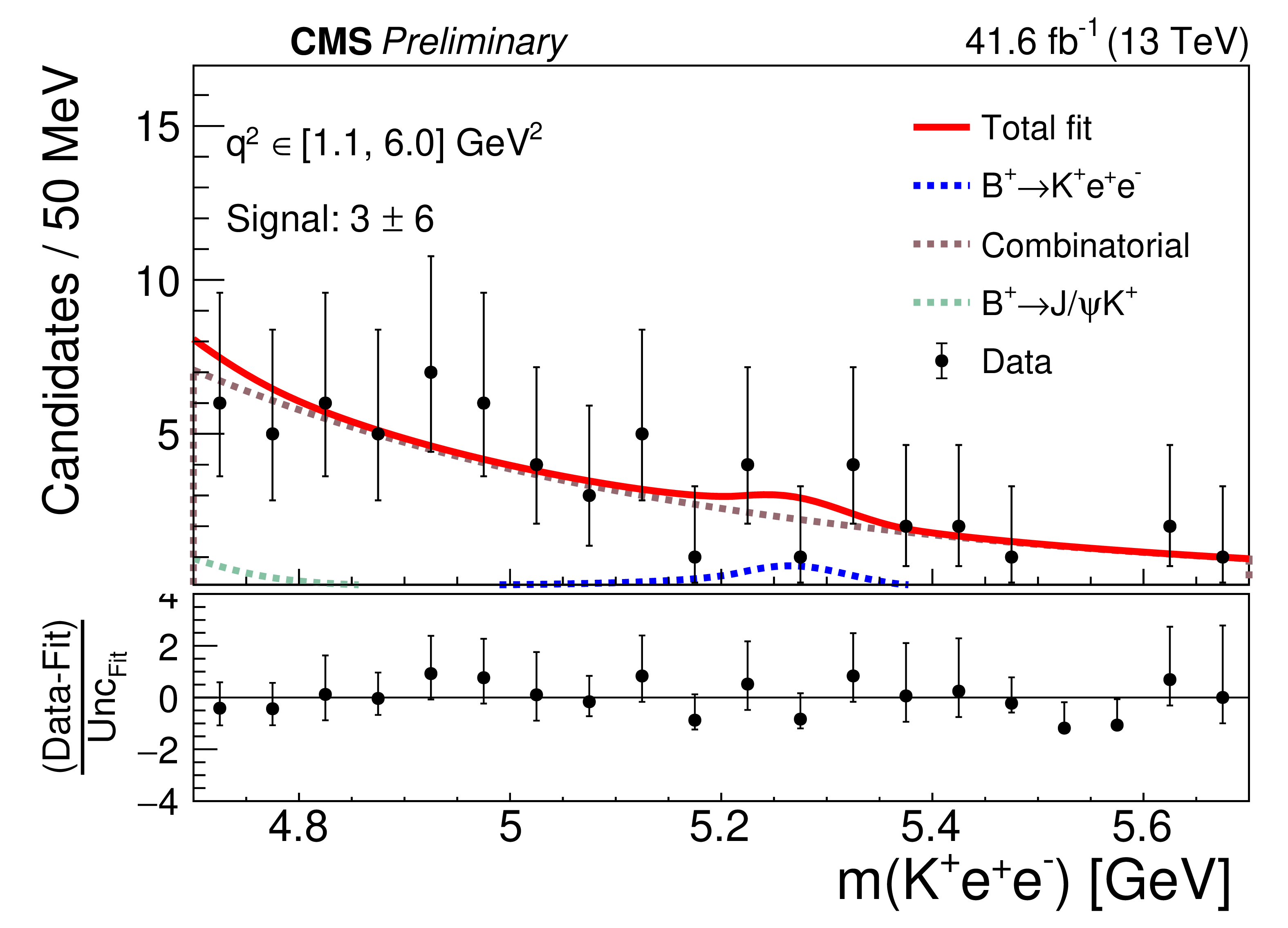
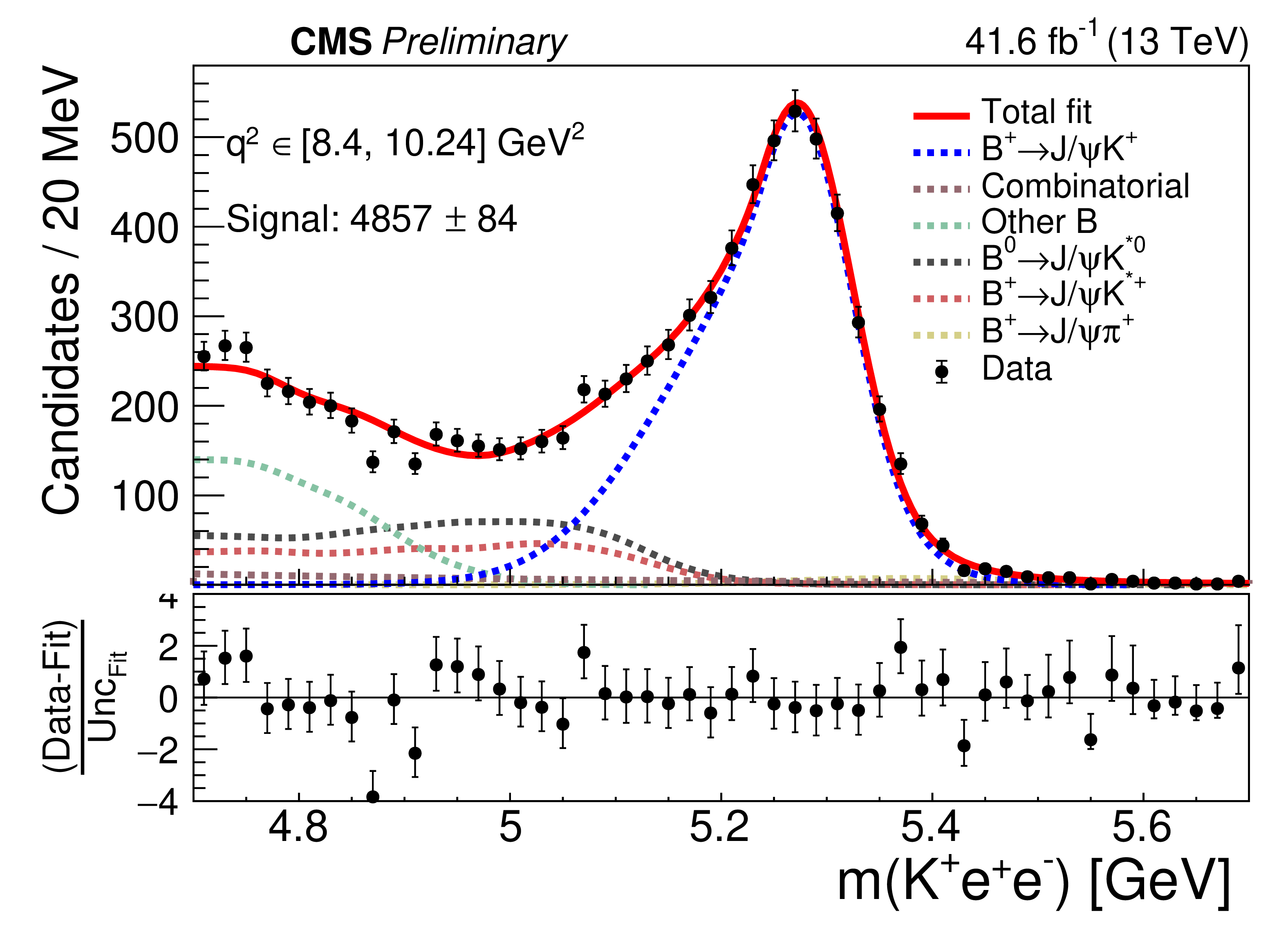
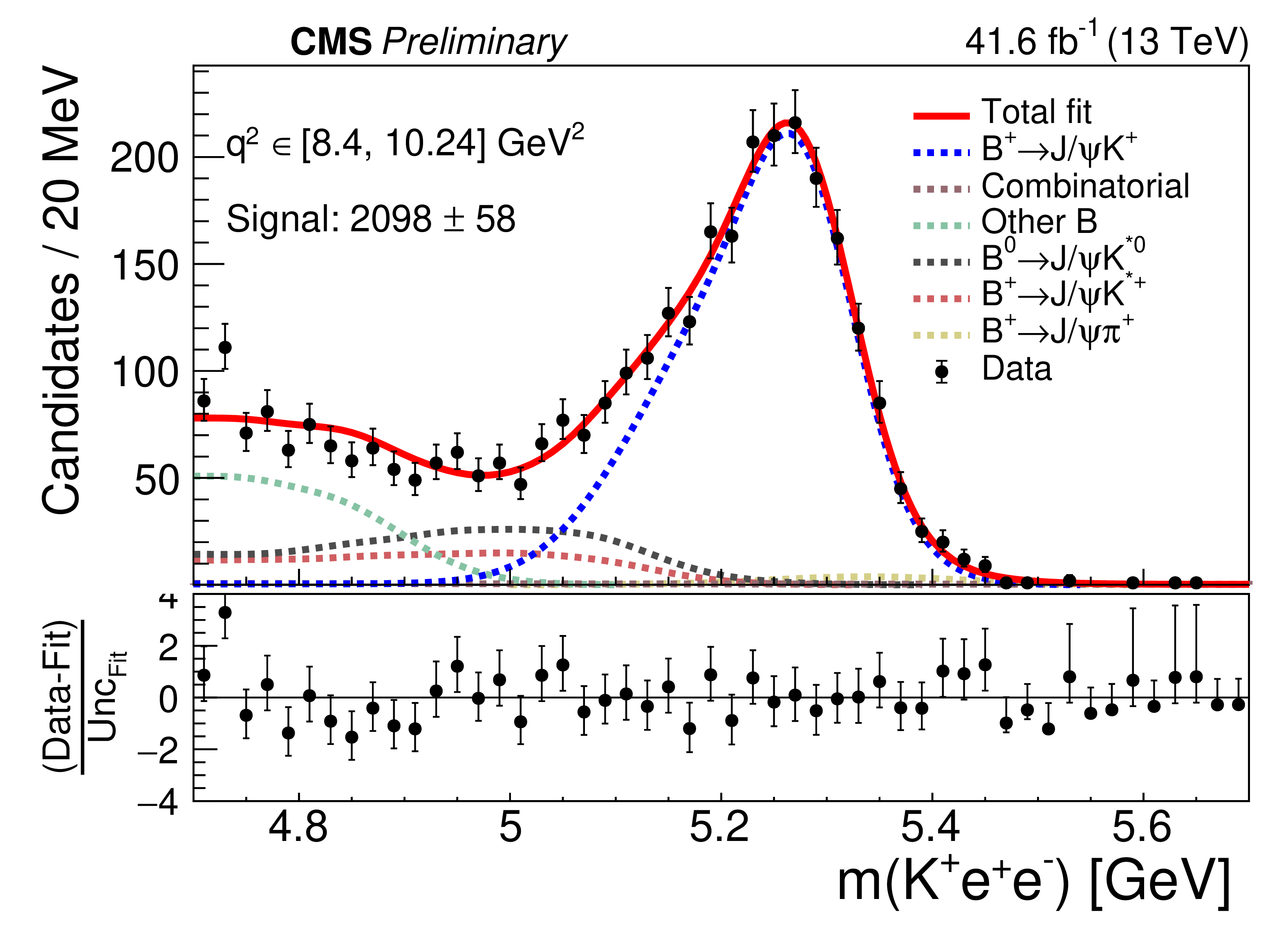
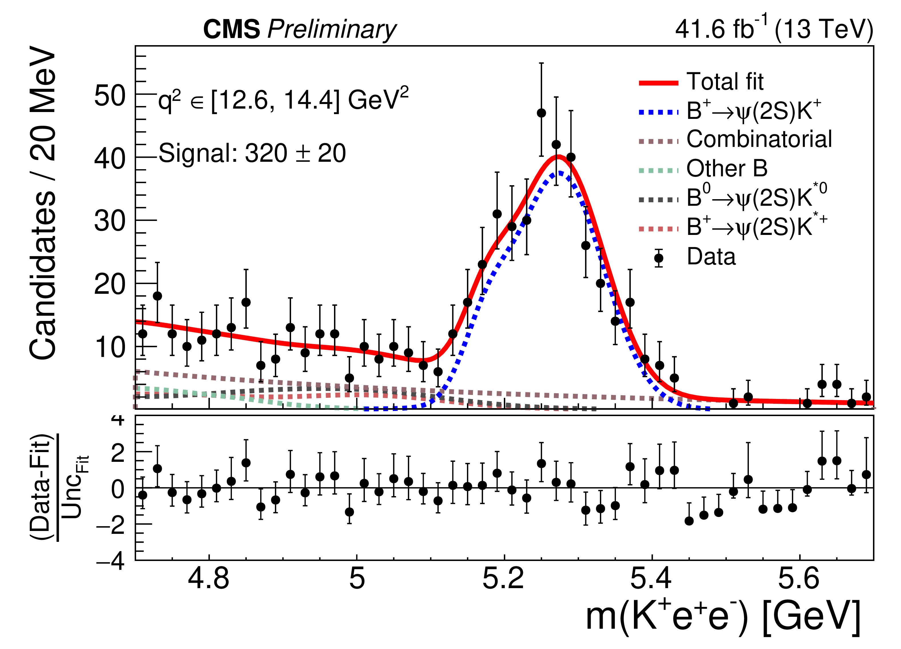
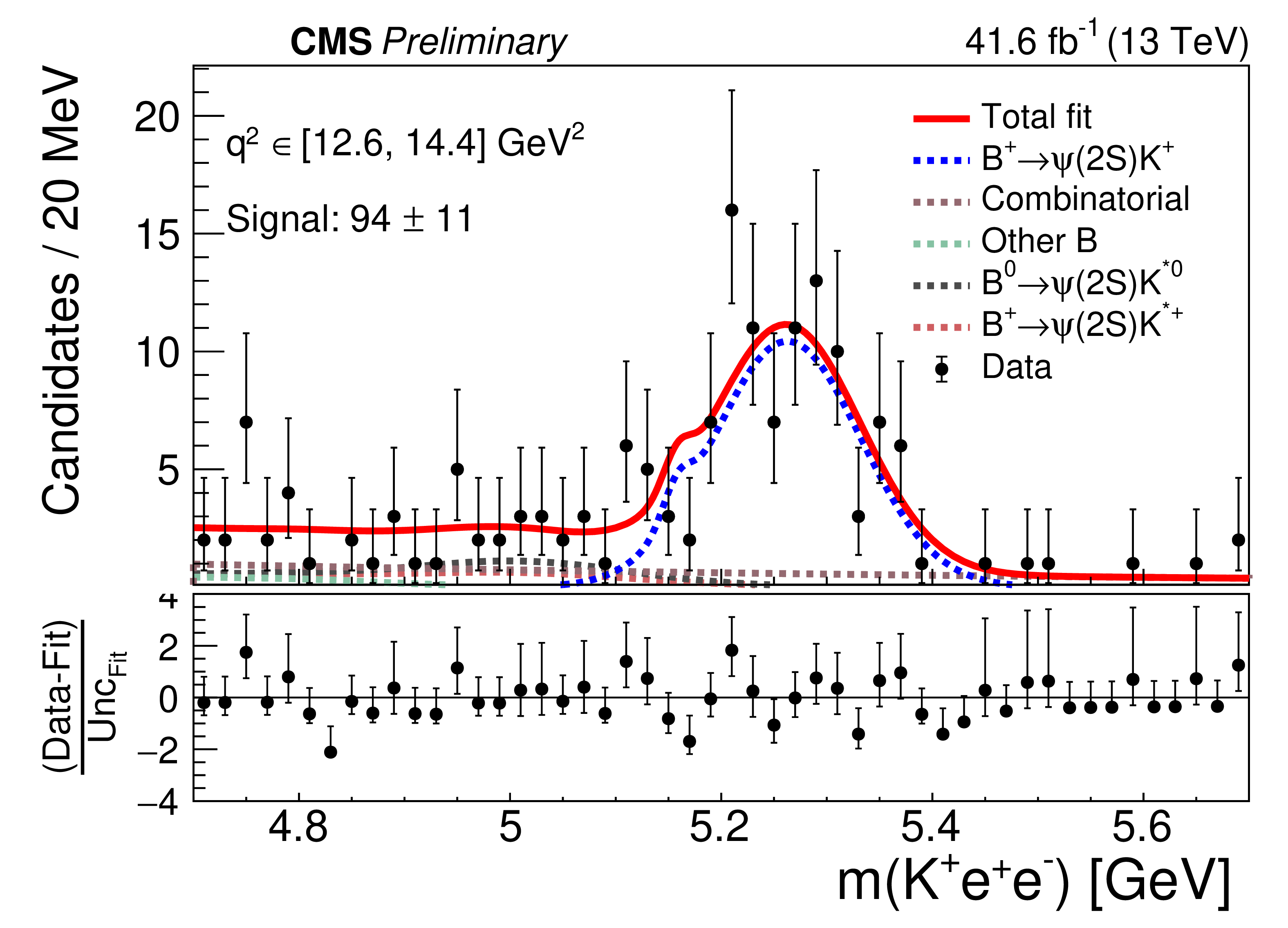
png pdf	Figure 8: The $\mathrm{K^+} \mathrm{e}^+ \mathrm{e}^-$ mass spectrum with the results of the fit show with the red line in the low-$q^2$ region (upper row), ${\mathrm{B}^{+}} \to {\mathrm{J}/\psi} (\mathrm{e}^+\mathrm{e}^-)\mathrm{K^+}$ control region (middle row), and ${\mathrm{B}^{+}} \to \psi(2\mathrm{S})(\mathrm{e}^+\mathrm{e}^-)\mathrm{K^+}$ control region (lower row) for the PF-PF (left) and PF-LP (right) categories. The shoulder below the nominal ${\mathrm{B}^{+}}$ meson mass for the $\psi(2\mathrm{S})$ control region is due to the narrow $q^2$ range in this bin. The lower panels show the distribution of the pull, which is defined as the difference between the data and the fit, divided by their combined uncertainty.
png pdf	Figure 8-a: The $\mathrm{K^+} \mathrm{e}^+ \mathrm{e}^-$ mass spectrum with the results of the fit show with the red line in the low-$q^2$ region (upper row), ${\mathrm{B}^{+}} \to {\mathrm{J}/\psi} (\mathrm{e}^+\mathrm{e}^-)\mathrm{K^+}$ control region (middle row), and ${\mathrm{B}^{+}} \to \psi(2\mathrm{S})(\mathrm{e}^+\mathrm{e}^-)\mathrm{K^+}$ control region (lower row) for the PF-PF (left) and PF-LP (right) categories. The shoulder below the nominal ${\mathrm{B}^{+}}$ meson mass for the $\psi(2\mathrm{S})$ control region is due to the narrow $q^2$ range in this bin. The lower panels show the distribution of the pull, which is defined as the difference between the data and the fit, divided by their combined uncertainty.
png pdf	Figure 8-b: The $\mathrm{K^+} \mathrm{e}^+ \mathrm{e}^-$ mass spectrum with the results of the fit show with the red line in the low-$q^2$ region (upper row), ${\mathrm{B}^{+}} \to {\mathrm{J}/\psi} (\mathrm{e}^+\mathrm{e}^-)\mathrm{K^+}$ control region (middle row), and ${\mathrm{B}^{+}} \to \psi(2\mathrm{S})(\mathrm{e}^+\mathrm{e}^-)\mathrm{K^+}$ control region (lower row) for the PF-PF (left) and PF-LP (right) categories. The shoulder below the nominal ${\mathrm{B}^{+}}$ meson mass for the $\psi(2\mathrm{S})$ control region is due to the narrow $q^2$ range in this bin. The lower panels show the distribution of the pull, which is defined as the difference between the data and the fit, divided by their combined uncertainty.
png pdf	Figure 8-c: The $\mathrm{K^+} \mathrm{e}^+ \mathrm{e}^-$ mass spectrum with the results of the fit show with the red line in the low-$q^2$ region (upper row), ${\mathrm{B}^{+}} \to {\mathrm{J}/\psi} (\mathrm{e}^+\mathrm{e}^-)\mathrm{K^+}$ control region (middle row), and ${\mathrm{B}^{+}} \to \psi(2\mathrm{S})(\mathrm{e}^+\mathrm{e}^-)\mathrm{K^+}$ control region (lower row) for the PF-PF (left) and PF-LP (right) categories. The shoulder below the nominal ${\mathrm{B}^{+}}$ meson mass for the $\psi(2\mathrm{S})$ control region is due to the narrow $q^2$ range in this bin. The lower panels show the distribution of the pull, which is defined as the difference between the data and the fit, divided by their combined uncertainty.
png pdf	Figure 8-d: The $\mathrm{K^+} \mathrm{e}^+ \mathrm{e}^-$ mass spectrum with the results of the fit show with the red line in the low-$q^2$ region (upper row), ${\mathrm{B}^{+}} \to {\mathrm{J}/\psi} (\mathrm{e}^+\mathrm{e}^-)\mathrm{K^+}$ control region (middle row), and ${\mathrm{B}^{+}} \to \psi(2\mathrm{S})(\mathrm{e}^+\mathrm{e}^-)\mathrm{K^+}$ control region (lower row) for the PF-PF (left) and PF-LP (right) categories. The shoulder below the nominal ${\mathrm{B}^{+}}$ meson mass for the $\psi(2\mathrm{S})$ control region is due to the narrow $q^2$ range in this bin. The lower panels show the distribution of the pull, which is defined as the difference between the data and the fit, divided by their combined uncertainty.
png pdf	Figure 8-e: The $\mathrm{K^+} \mathrm{e}^+ \mathrm{e}^-$ mass spectrum with the results of the fit show with the red line in the low-$q^2$ region (upper row), ${\mathrm{B}^{+}} \to {\mathrm{J}/\psi} (\mathrm{e}^+\mathrm{e}^-)\mathrm{K^+}$ control region (middle row), and ${\mathrm{B}^{+}} \to \psi(2\mathrm{S})(\mathrm{e}^+\mathrm{e}^-)\mathrm{K^+}$ control region (lower row) for the PF-PF (left) and PF-LP (right) categories. The shoulder below the nominal ${\mathrm{B}^{+}}$ meson mass for the $\psi(2\mathrm{S})$ control region is due to the narrow $q^2$ range in this bin. The lower panels show the distribution of the pull, which is defined as the difference between the data and the fit, divided by their combined uncertainty.
png pdf	Figure 8-f: The $\mathrm{K^+} \mathrm{e}^+ \mathrm{e}^-$ mass spectrum with the results of the fit show with the red line in the low-$q^2$ region (upper row), ${\mathrm{B}^{+}} \to {\mathrm{J}/\psi} (\mathrm{e}^+\mathrm{e}^-)\mathrm{K^+}$ control region (middle row), and ${\mathrm{B}^{+}} \to \psi(2\mathrm{S})(\mathrm{e}^+\mathrm{e}^-)\mathrm{K^+}$ control region (lower row) for the PF-PF (left) and PF-LP (right) categories. The shoulder below the nominal ${\mathrm{B}^{+}}$ meson mass for the $\psi(2\mathrm{S})$ control region is due to the narrow $q^2$ range in this bin. The lower panels show the distribution of the pull, which is defined as the difference between the data and the fit, divided by their combined uncertainty.
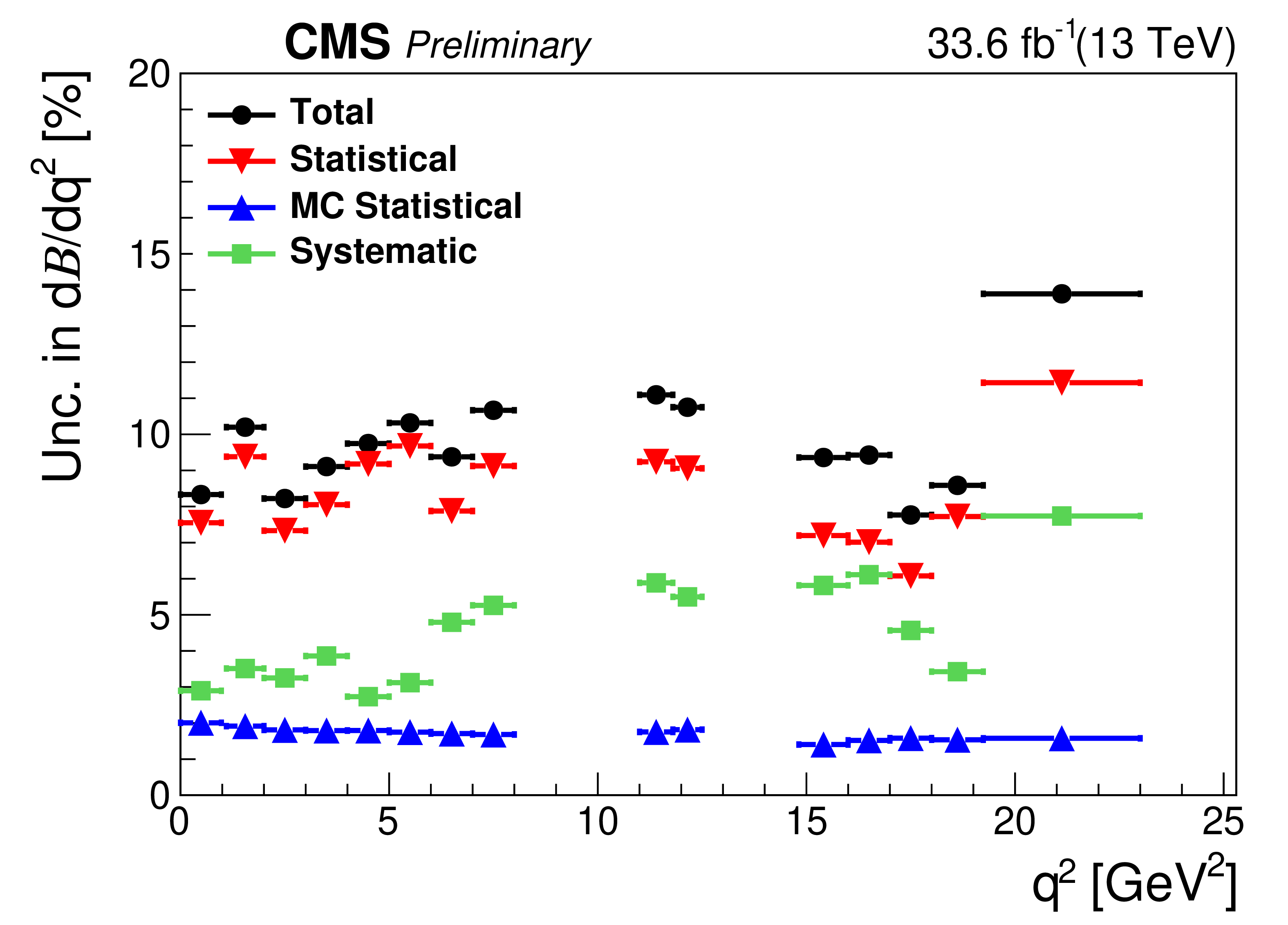
png pdf	Figure 9: Relative uncertainties in the differential branching fraction per $q^2$ bin. Different colors correspond to statistical, simulation statistical, and systematic uncertainties.
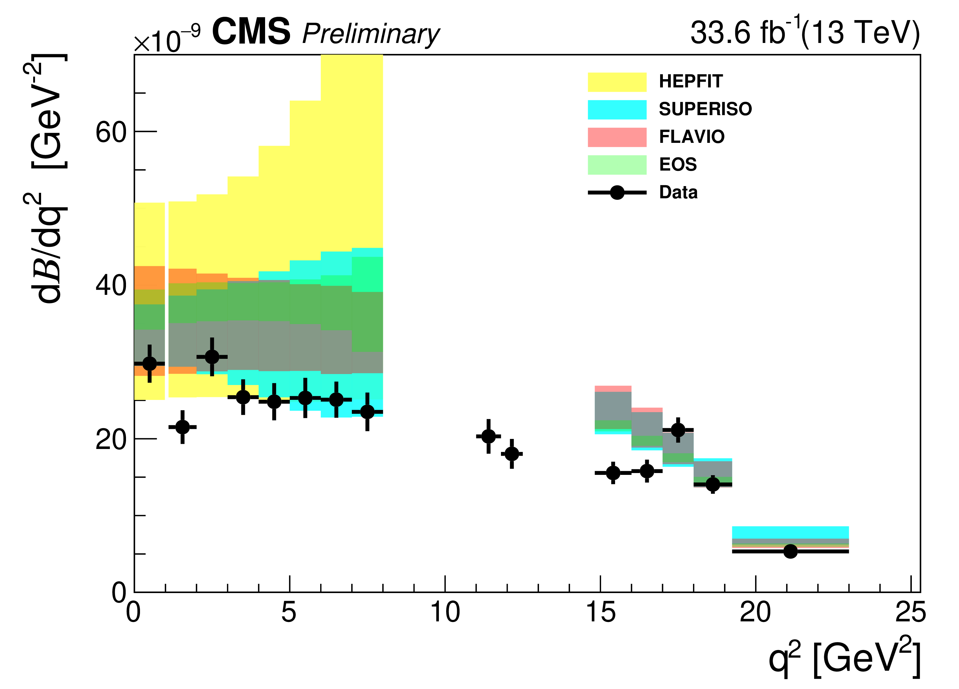
png pdf	Figure 10: Comparison of the measured differential ${\mathrm{B}^{+}} \to \mathrm{K^+}\mu^{+}\mu^{-}$ branching fraction with the theoretical predictions obtained using FLAVIO, SUPERISO, HEPFIT, and EOS packages.
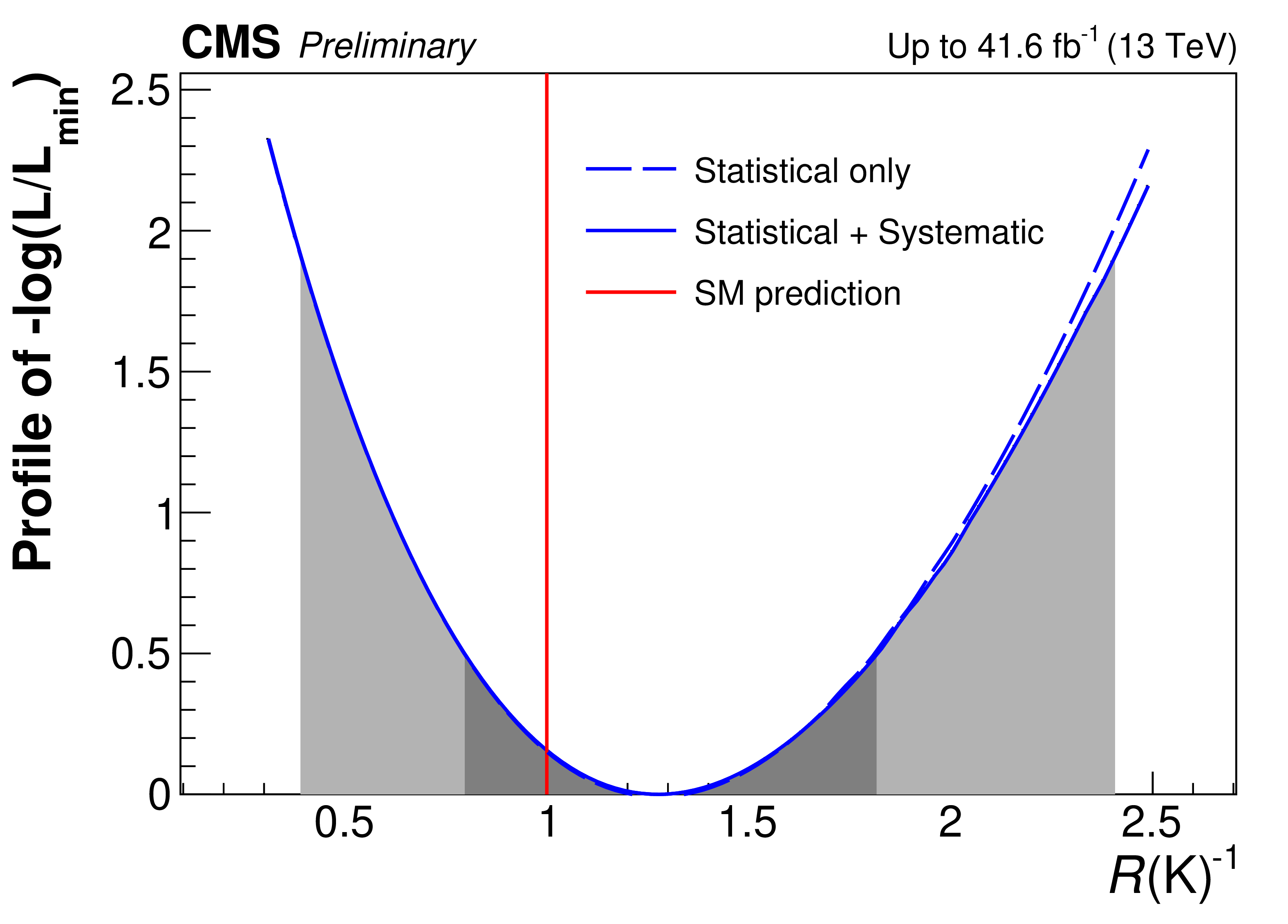
png pdf	Figure 11: Likelihood function from the fit profiled as a function of $R(\mathrm{K})^{-1}$.

Tables
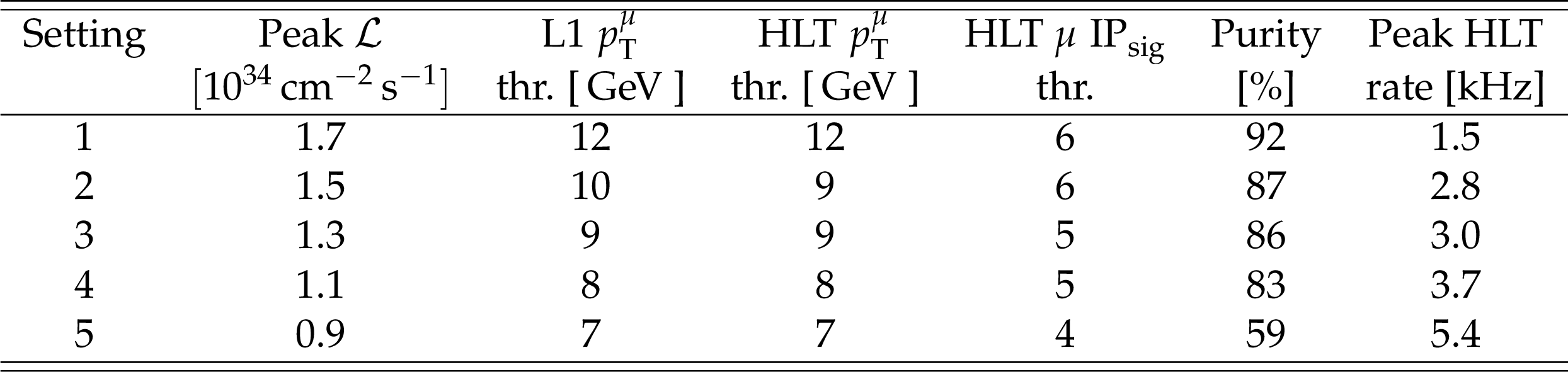
png pdf	Table 1: Summary of the loosest muon trigger requirements imposed by the L1 and HLT algorithms for each instantaneous luminosity scenario: the L1 and HLT muon transverse momentum thresholds $p^\mu_{\mathrm{T}}$, and the HLT muon impact parameter significance $\text{IP}_{\text{sig}}$, defined as the impact parameter in the plane perpendicular to the beams divided by its uncertainty. Also shown are the trigger purity and peak HLT rate. All values are shown in bins of the peak instantaneous luminosity $\mathcal{L}$.
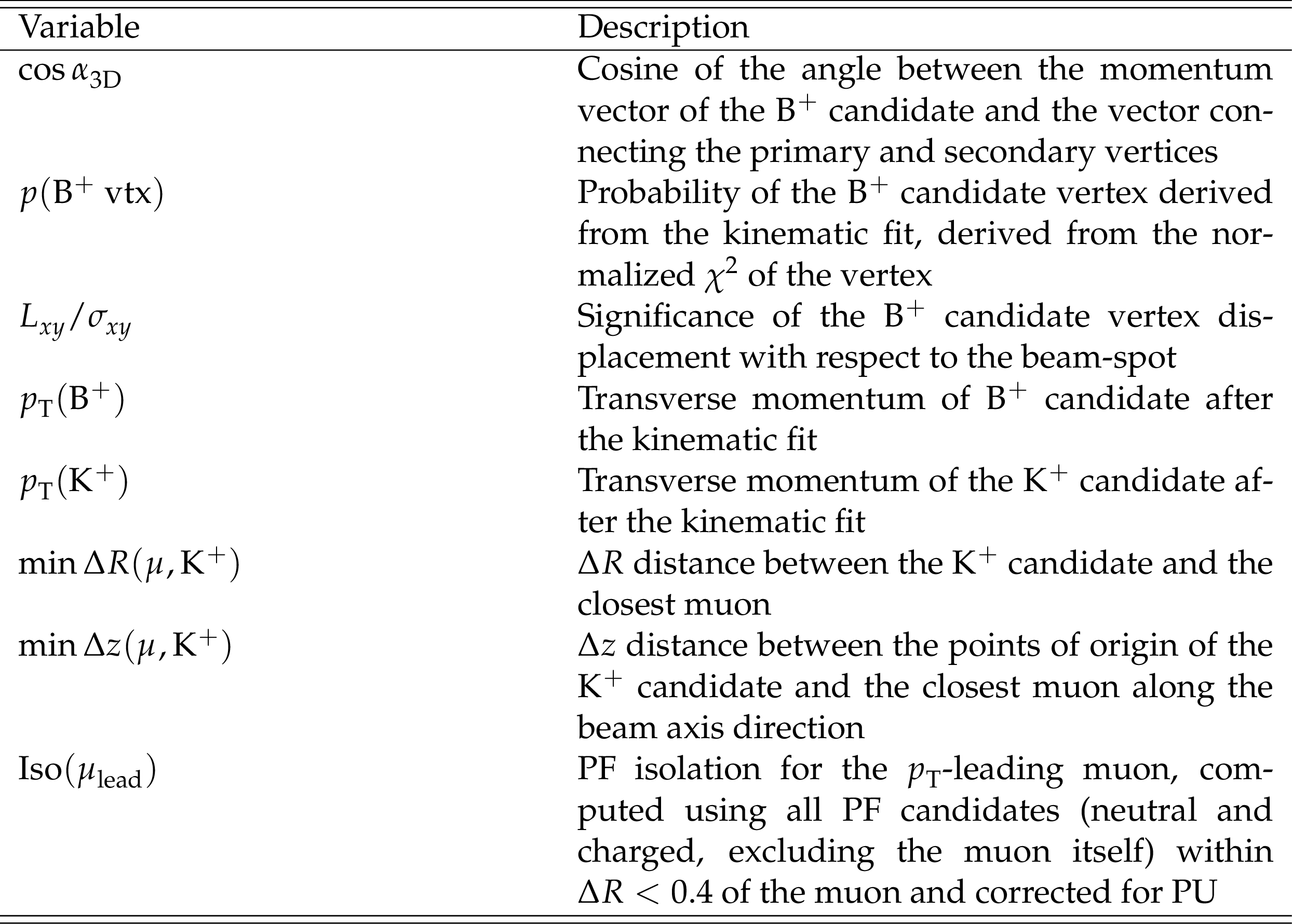
png pdf	Table 2: Input variables used in the muon channel BDT.
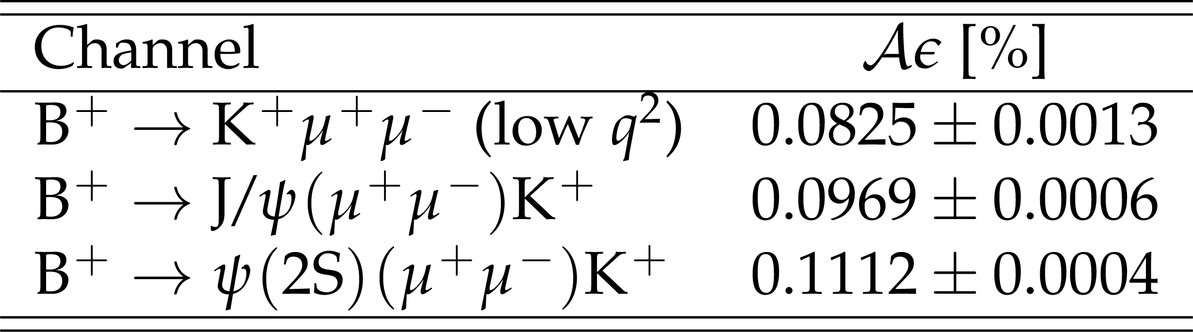
png pdf	Table 3: The product of acceptance and efficiency (${\cal A}\epsilon$) for the muon channel for the signal in the low-$q^2$ bin and for the ${\mathrm{B}^{+}} \to {\mathrm{J}/\psi} (\mu^{+}\mu^{-})\mathrm{K^+}$ control sample.
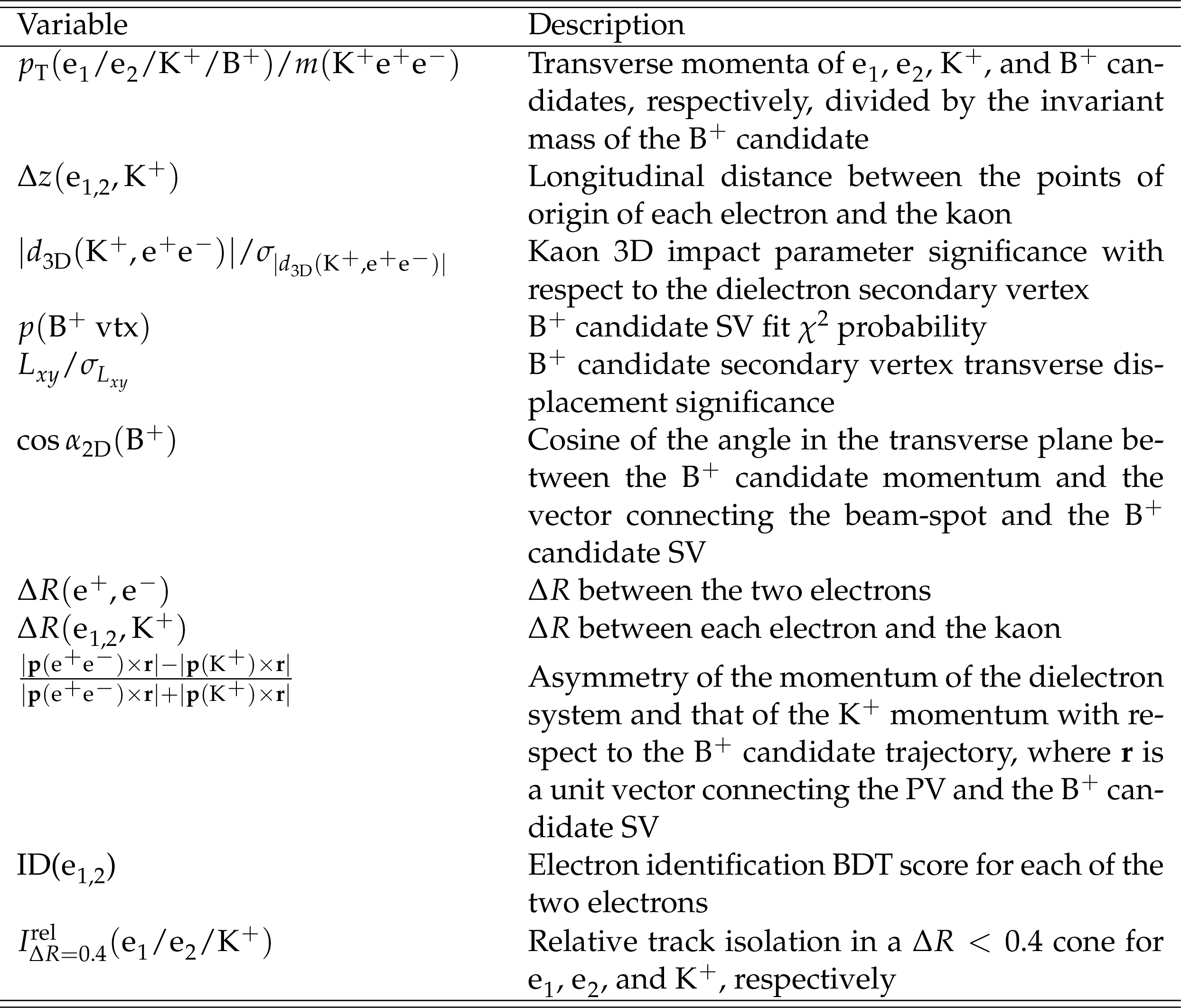
png pdf	Table 4: Input variables used in the electron channel BDTs, for both PF-PF and PF-LP categories.
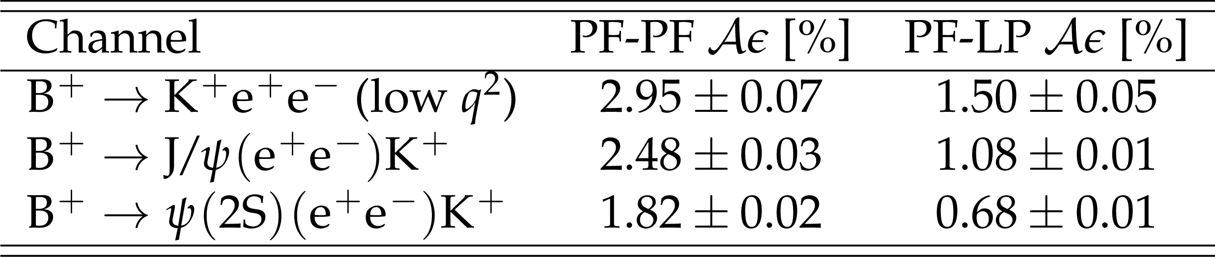
png pdf	Table 5: The product of acceptance and efficiency (${\cal A}\epsilon$) for the electron channel for the signal in the low-$q^2$ bin, and for the ${\mathrm{B}^{+}} \to {\mathrm{J}/\psi} (\mathrm{e}^+\mathrm{e}^-)\mathrm{K^+}$ and ${\mathrm{B}^{+}} \to \psi(2\mathrm{S})(\mathrm{e}^+\mathrm{e}^-)\mathrm{K^+}$ control regions in the PF-PF and PF-LP categories. Trigger efficiency is not included in the quoted numbers, and they represent the average across the corresponding $q^2$ bin.
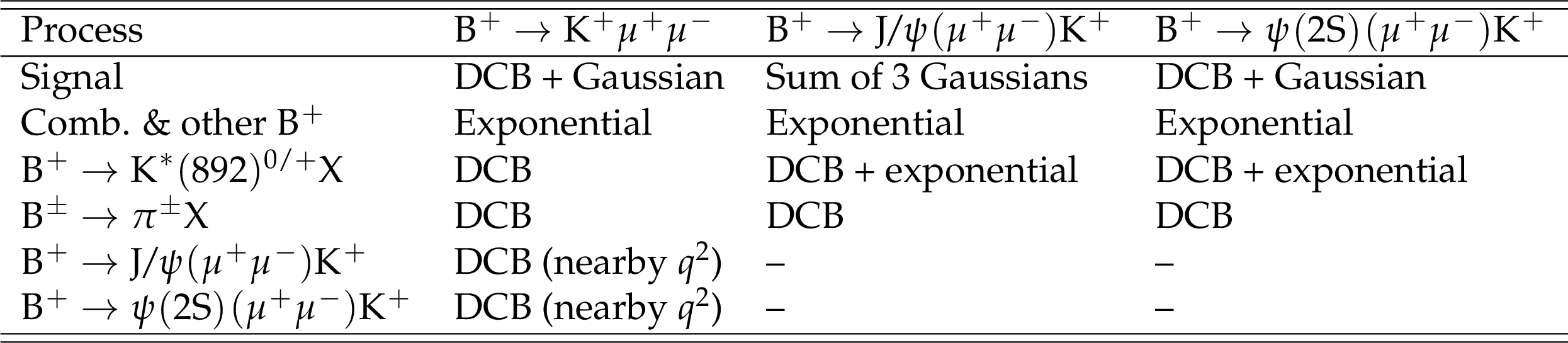
png pdf	Table 6: Fit functions used for signal and background sources in each $q^2$ bin. The ``--" symbol indicates that the corresponding background does not apply in this channel.
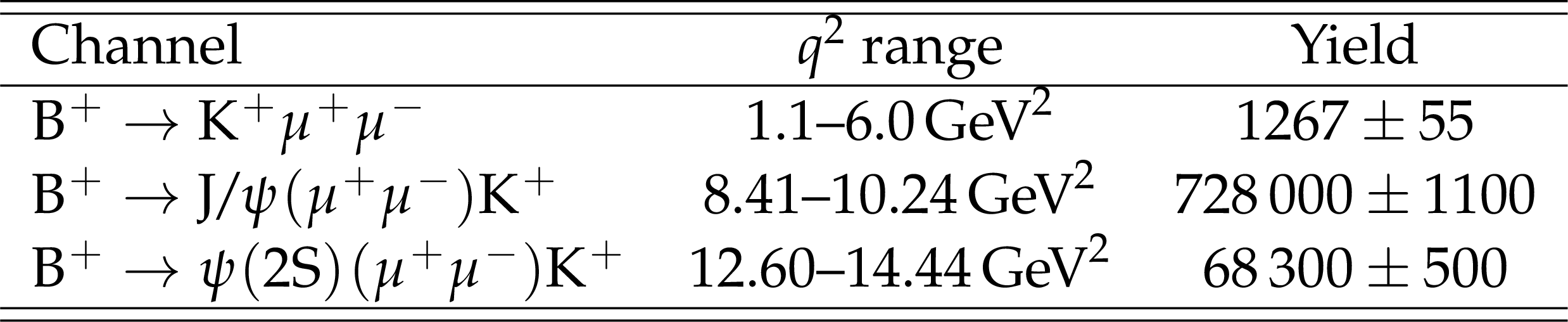
png pdf	Table 7: Event yields in the muon channel.
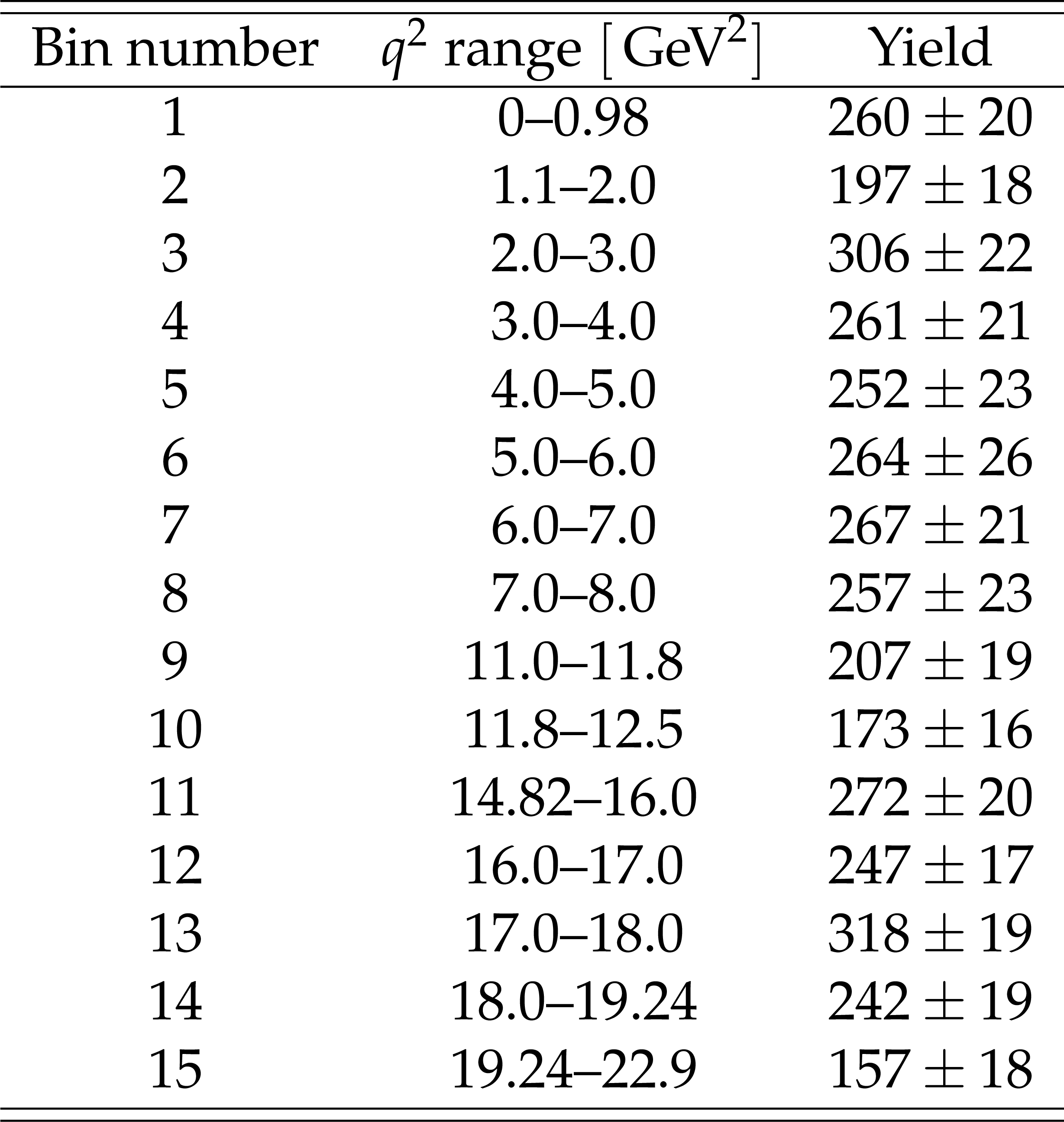
png pdf	Table 8: Yields per $q^2$ bin extracted from the simultaneous fit in the ${\mathrm{B}^{+}} \to \mathrm{K^+}\mu^{+}\mu^{-}$ channel. The uncertainties shown are statistical uncertainties from the fit.
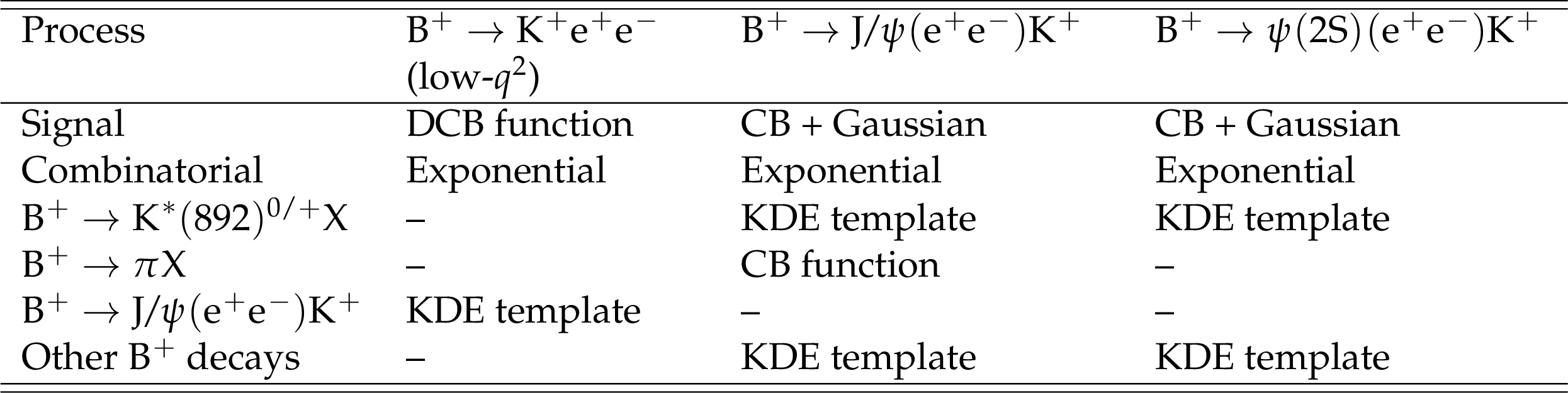
png pdf	Table 9: Fit functions used to describe signal and various background components for the electron channel. The ``--'' sign implies that the specific source of the background is not relevant in this region.
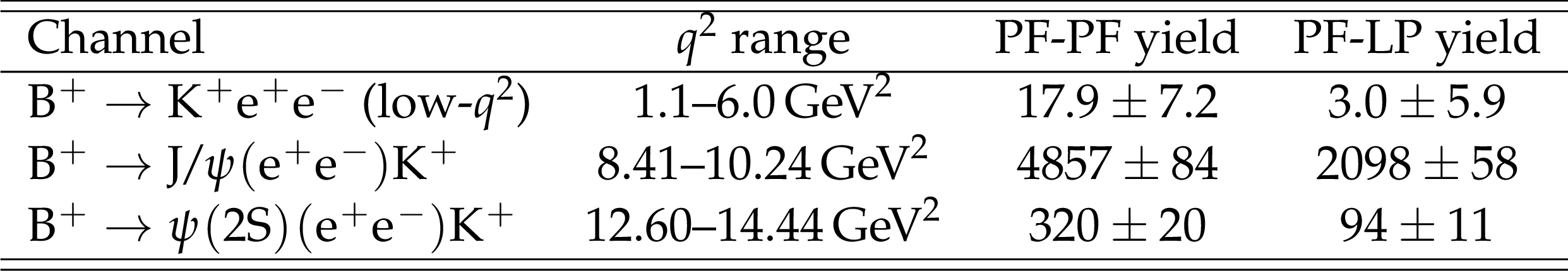
png pdf	Table 10: Signal yields in the electron channel in the low-$q^2$ bin and resonant CRs, for both PF-PF and PF-LP categories.
png pdf	Table 11: Major sources of uncertainty in the ${\mathrm{B}^{+}} \to \mathrm{K^+}\mu^{+}\mu^{-}$/${\mathrm{B}^{+}} \to {\mathrm{J}/\psi} (\mu^{+}\mu^{-})\mathrm{K^+}$ ratio measurement.
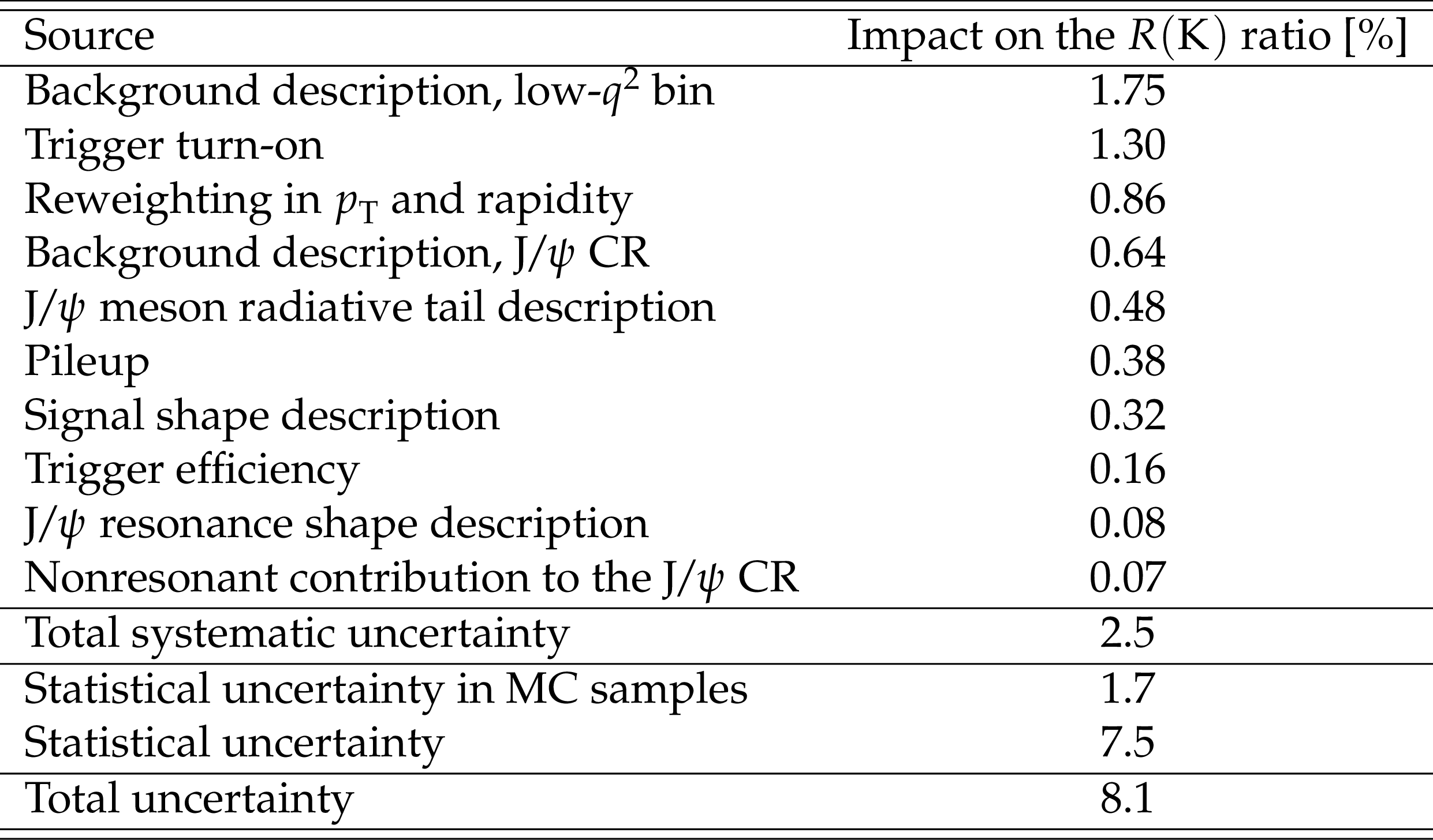
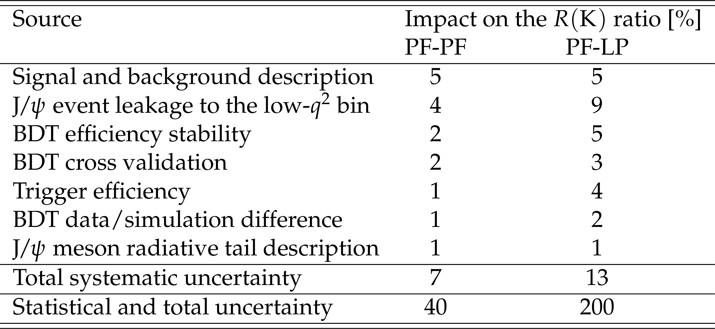
png pdf	Table 12: Major sources of uncertainty in the ${\mathrm{B}^{+}} \to \mathrm{K^+}\mathrm{e}^+\mathrm{e}^-$/${\mathrm{B}^{+}} \to {\mathrm{J}/\psi} (\mathrm{e}^+\mathrm{e}^-)\mathrm{K^+}$ ratio measurement in the PF-PF and PF-LP categories. The last row shows the statistical uncertainty, which is the same as the total uncertainty within the quoted precision.
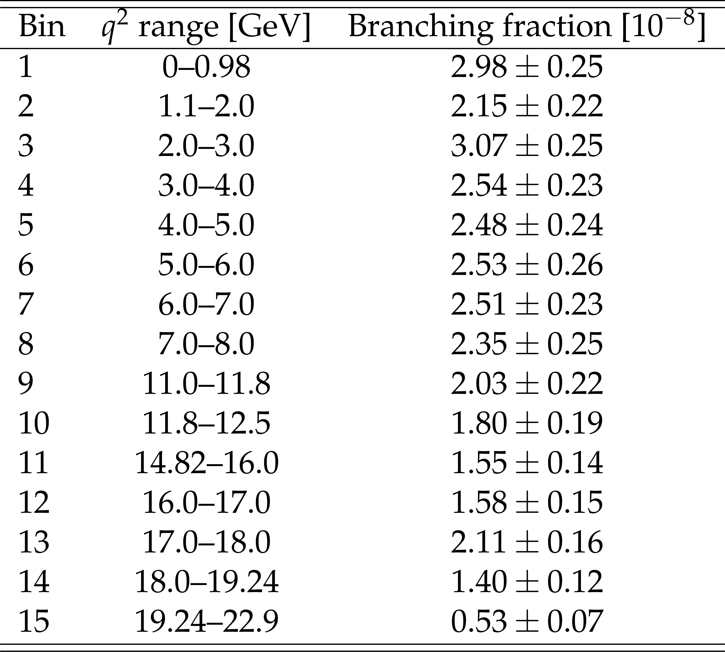
png pdf	Table 13: The differential ${\mathrm{B}^{+}} \to \mathrm{K^+}\mu^{+}\mu^{-}$ branching fraction measured in the individual $q^2$ bins. The uncertainties include both the statistical and systematic components.
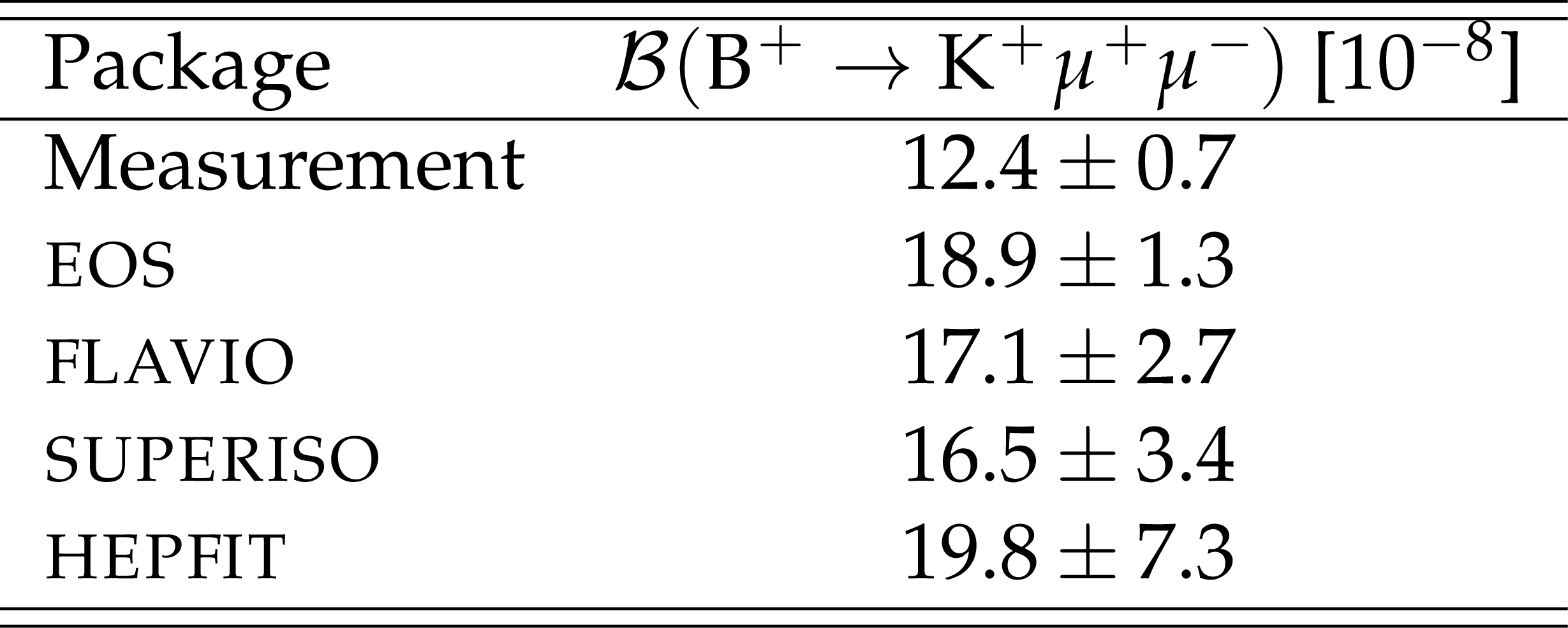
png pdf	Table 14: Comparison of the branching fraction $\mathcal{B}({\mathrm{B}^{+}} \to \mathrm{K^+}\mu^{+}\mu^{-})$ measurement in the low-$q^2$ bin and the theoretical predictions based on the EOS, FLAVIO, SUPERISO, and HEPFIT packages.. The HEPFIT predictions are only available for $q^2 <$ 8 GeV$^2$.
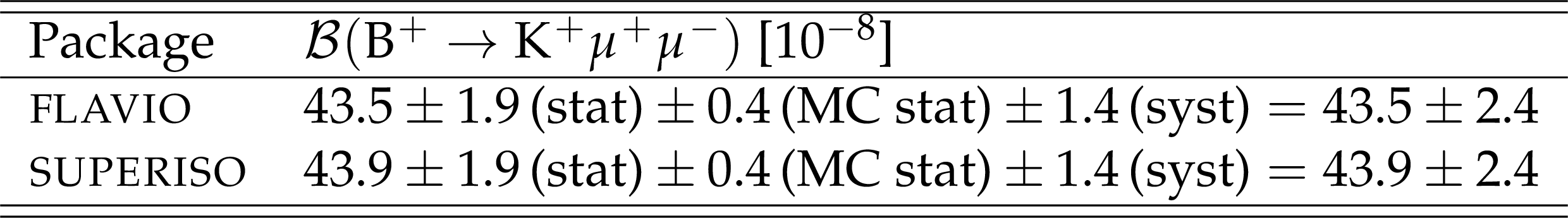
png pdf	Table 15: Measurement of the inclusive branching fraction $\mathcal{B}({\mathrm{B}^{+}} \to \mathrm{K^+}\mu^{+}\mu^{-})$ using theoretical calculations based on the FLAVIO and SUPERISO packages. The theoretical uncertainty is not included.

Summary

In summary, we reported the first test of lepton flavor universality in ${\mathrm{B}^{\pm}} \to \mathrm{K^{\pm}}\ell^+\ell^-$ decays, where $\ell$ is a muon or electron, as well as a measurement of differential and inclusive branching fractions of a nonresonant ${\mathrm{B}^{\pm}} \to \mathrm{K^{\pm}}\mu^{+}\mu^{-}$ decay with the CMS experiment at the LHC. The analysis was made possible by a dedicated data set of proton-proton collisions at $\sqrt{s} =$ 13 TeV recorded in 2018, using a special high-rate data stream designed for collecting about 10 billion unbiased b hadron decays. The ratio of the branching fractions $\mathcal{B}({\mathrm{B}^{\pm}} \to \mathrm{K^{\pm}}\mu^{+}\mu^{-})$ to $\mathcal{B}({\mathrm{B}^{\pm}} \to \mathrm{K^{\pm}}\mathrm{e}^+\mathrm{e}^-)$ was measured as a double ratio $R(\mathrm{K})$ of these decays to the respective branching fractions of the ${\mathrm{B}^{\pm}} \to {\mathrm{J}/\psi} \mathrm{K^{\pm}} ({\mathrm{J}/\psi} \to\mu^{+}\mu^{-})$ and $({\mathrm{J}/\psi} \to\mathrm{e}^+\mathrm{e}^-)$ decays, which allow for significant cancellation of systematic uncertainties. The ratio $R(\mathrm{K})$ was measured in a range 1.1 $< q^2 <$ 6.0 GeV$^2$, where $q$ is the invariant mass of the lepton pair, and was found to be $R(\mathrm{K})=$ 0.78 $^{+0.47}_{-0.23}$, in agreement with the standard model expectation within one standard deviation. This measurement is limited by the statistical precision of the electron channel. The inclusive branching fraction in the same $q^2$ range of $\mathcal{B}({\mathrm{B}^{\pm}} \to \mathrm{K^{\pm}}\mu^{+}\mu^{-}) =$ ( 12.42 $\pm$ 0.54 (stat) $\pm$ 0.11 (MC stat) $\pm$ 0.40 (syst) ) $\times$ 10$^{-8}$ is consistent with and has a comparable precision to the present world average. This work demonstrates the flexibility of the CMS trigger and its data acquisition system and paves the way to many other studies of a large unbiased sample of b hadron decays collected by CMS at the end of the LHC Run 2.

References
1	S. L. Glashow	Partial Symmetries of Weak Interactions	NP 22 (1961) 579
2	S. Weinberg	A Model of Leptons	PRL 19 (1967) 1264
3	A. Salam	Weak and Electromagnetic Interactions	N. Svartholm (Ed.), Proc. 8-th Nobel Symp., Almquist and Wiksell, 1968 Stockholm 36 (1968) 7
4	Particle Data Group Collaboration	Review of Particle Physics	PTEP 2022 (2022) 083C01
5	ALEPH, DELPHI, L3, OPAL, LEP Electroweak Collaboration	Electroweak Measurements in Electron-Positron Collisions at W-Boson-Pair Energies at LEP	Phys. Rept. 532 (2013) 119	1302.3415
6	ATLAS Collaboration	Test of the universality of $\tau$ and $\mu$ lepton couplings in $W$-boson decays with the ATLAS detector	Nature Phys. 17 (2021) 813	2007.14040
7	CMS Collaboration	Precision measurement of the W boson decay branching fractions in proton-proton collisions at $\sqrt{s}$ = 13 TeV	PRD 105 (2022) 072008	CMS-SMP-18-011 2201.07861
8	D. London and J. Matias	$B$ Flavour Anomalies: 2021 Theoretical Status Report	Ann. Rev. Nucl. Part. Sci. 72 (2022) 37	2110.13270
9	LHCb Collaboration	Test of lepton universality in beauty-quark decays	Nature Phys. 18 (2022) 277	2103.11769
10	LHCb Collaboration	Test of lepton universality using $B^{+}\rightarrow K^{+}\ell^{+}\ell^{-}$ decays	PRL 113 (2014) 151601	1406.6482
11	LHCb Collaboration	Test of lepton universality with $B^{0} \rightarrow K^{*0}\ell^{+}\ell^{-}$ decays	JHEP 08 (2017) 055	1705.05802
12	LHCb Collaboration	Tests of lepton universality using $B^0\to K^0_S \ell^+ \ell^-$ and $B^+\to K^{*+} \ell^+ \ell^-$ decays	PRL 128 (2022) 191802	2110.09501
13	LHCb Collaboration	Measurement of the isospin asymmetry in $B \to K^{(*)}\mu^+\mu^-$ decays	JHEP 07 (2012) 133	1205.3422
14	LHCb Collaboration	Differential branching fractions and isospin asymmetries of $B \to K^{(*)} \mu^+ \mu^-$ decays	JHEP 06 (2014) 133	1403.8044
15	LHCb Collaboration	Measurements of the S-wave fraction in $B^{0}\rightarrow K^{+}\pi^{-}\mu^{+}\mu^{-}$ decays and the $B^{0}\rightarrow K^{\ast}(892)^{0}\mu^{+}\mu^{-}$ differential branching fraction	[Erratum: \doi10./JHEP04()142], 2016 JHEP 11 (2016) 047	1606.04731
16	LHCb Collaboration	Branching Fraction Measurements of the Rare $B^0_s\rightarrow\phi\mu^+\mu^-$ and $B^0_s\rightarrow f_2^\prime(1525)\mu^+\mu^-$- Decays	PRL 127 (2021) 151801	2105.14007
17	M. Ciuchini et al.	Charming penguins and lepton universality violation in $b \rightarrow s \ell ^+ \ell ^-$ decays	EPJC 83 (2023) 64	2110.10126
18	LHCb Collaboration	Test of lepton universality in $b \rightarrow s \ell^+ \ell^-$ decays	PRL 131 (2023) 051803	2212.09152
19	LHCb Collaboration	Measurement of lepton universality parameters in $B^+\to K^+\ell^+\ell^-$ and $B^0\to K^{*0}\ell^+\ell^-$ decays	PRD 108 (2023) 032002	2212.09153
20	M. Bordone, G. Isidori, and A. Pattori	On the Standard Model predictions for $R_K$ and $R_{K^*}$	EPJC 76 (2016) 440	1605.07633
21	G. Isidori, S. Nabeebaccus, and R. Zwicky	QED corrections in $\overline{B}\to \overline{K}{\mathrm{\ell}}^{+}{\mathrm{\ell}}^{-}$ at the double-differential level	JHEP 12 (2020) 104	2009.00929
22	G. Isidori, D. Lancierini, S. Nabeebaccus, and R. Zwicky	QED in $\overline{B} \to \overline{K}$\ensuremath\ell$^{+}$\ensuremath\ell$^{-}$ LFU ratios: theory versus experiment, a Monte Carlo study	JHEP 10 (2022) 146	2205.08635
23	CMS Collaboration	Recording and reconstructing 10 billion unbiased b hadron decays in CMS	CMS Detector Performance Summary CMS-DP-2019-043, 2019 CDS
24	CMS Collaboration	CMS luminosity measurements for the 2018 data-taking period at $\sqrt{s} =$ 13 TeV	CMS Physics Analysis Summary, 2018 CMS-PAS-LUM-18-001	CMS-PAS-LUM-18-001
25	T. Sj\"ostrand et al.	An introduction to PYTHIA 8.2	Comput. Phys. Commun. 191 (2015) 159	1410.3012
26	CMS Collaboration	Extraction and validation of a new set of CMS PYTHIA8 tunes from underlying-event measurements	EPJC 80 (2020) 4	CMS-GEN-17-001 1903.12179
27	NNPDF Collaboration	Parton distributions from high-precision collider data	EPJC 77 (2017) 663	1706.00428
28	D. J. Lange	The EvtGen particle decay simulation package	NIM A 462 (2001) 152
29	E. Barberio and Z. Was	PHOTOS: A Universal Monte Carlo for QED radiative corrections. Version 2.0	Comput. Phys. Commun. 79 (1994) 291
30	GEANT4 Collaboration	GEANT 4---a simulation toolkit	NIM A 506 (2003) 250
31	CMS Collaboration	Performance of the CMS muon detector and muon reconstruction with proton-proton collisions at $\sqrt{s}=$ 13 TeV	JINST 13 (2018) P06015	CMS-MUO-16-001 1804.04528
32	CMS Collaboration	CMS Tracking Performance Results from Early LHC Operation	EPJC 70 (2010) 1165	CMS-TRK-10-001 1007.1988
33	CMS Collaboration	Particle-flow reconstruction and global event description with the CMS detector	JINST 12 (2017) P10003	CMS-PRF-14-001 1706.04965
34	CMS Collaboration	Electron and photon reconstruction and identification with the CMS experiment at the CERN LHC	JINST 16 (2021) P05014	CMS-EGM-17-001 2012.06888
35	K. Prokofiev and T. Speer	A Kinematic fit and a decay chain reconstruction library	/020, 2004 CMS Note 200 (2004) 4
36	T. Chen and C. Guestrin	XGBoost: a scalable tree boosting system		1603.02754
37	M. Pivk and F. R. Le Diberder	SPlot: A Statistical tool to unfold data distributions	NIM A 555 (2005) 356	physics/0402083
38	CMS Collaboration	Measurement of the Inclusive $W$ and $Z$ Production Cross Sections in $pp$ Collisions at $\sqrt{s}=$ 7 TeV	JHEP 10 (2011) 132	CMS-EWK-10-005 1107.4789
39	M. Cacciari, M. Greco, and P. Nason	The P(T) spectrum in heavy flavor hadroproduction	JHEP 05 (1998) 007	hep-ph/9803400
40	M. Cacciari, S. Frixione, and P. Nason	The p(T) spectrum in heavy flavor photoproduction	JHEP 03 (2001) 006	hep-ph/0102134
41	M. Cacciari et al.	Theoretical predictions for charm and bottom production at the LHC	JHEP 10 (2012) 137	1205.6344
42	M. Cacciari, M. L. Mangano, and P. Nason	Gluon PDF constraints from the ratio of forward heavy-quark production at the LHC at $\sqrt{S}=$ 7 and 13 TeV	EPJC 75 (2015) 610	1507.06197
43	M. J. Oreglia	A study of the reactions $\psi^\prime \to \gamma \gamma \psi$	PhD thesis, Stanford University, . SLAC Report SLAC-R-236, 1980 link
44	J. E. Gaiser	Charmonium spectroscopy from radiative decays of $\mathrm{J}/\psi$ and $\psi'$	PhD thesis, Stanford University, . SLAC Report SLAC-R-255, 1982 link
45	K. S. Cranmer	Kernel estimation in high-energy physics	Comput. Phys. Commun. 136 (2001) 198	hep-ex/0011057
46	CMS Collaboration	Measurement of the inelastic proton-proton cross section at $\sqrt{s}=$ 13 TeV	JHEP 07 (2018) 161	CMS-FSQ-15-005 1802.02613
47	EOS Authors Collaboration	EOS: a software for flavor physics phenomenology	EPJC 82 (2022) 569	2111.15428
48	N. Gubernari, M. Reboud, D. van Dyk, and J. Virto	Improved theory predictions and global analysis of exclusive $b \to s\mu^+\mu^-$ processes	JHEP 09 (2022) 133	2206.03797
49	D. M. Straub	flavio: a Python package for flavour and precision phenomenology in the Standard Model and beyond		1810.08132
50	F. Mahmoudi	SuperIso: A Program for calculating the isospin asymmetry of B ---\ensuremath> K* gamma in the MSSM	Comput. Phys. Commun. 178 (2008) 745	0710.2067
51	F. Mahmoudi	SuperIso v2.3: A Program for calculating flavor physics observables in Supersymmetry	Comput. Phys. Commun. 180 (2009) 1579	0808.3144
52	J. De Blas et al.	$\texttt{HEPfit}$: a code for the combination of indirect and direct constraints on high energy physics models	EPJC 80 (2020) 456	1910.14012
53	L. Alasfar et al.	$B$ anomalies under the lens of electroweak precision	JHEP 12 (2020) 016	2007.04400
54	M. Ciuchini et al.	Constraints on lepton universality violation from rare B decays	PRD 107 (2023) 055036	2212.10516
55	N. Gubernari, M. Reboud, D. van Dyk, and J. Virto	Dispersive Analysis of $B\to K^{(*)}$ and $B_s\to \phi$ Form Factors		2305.06301
56	LHCb Collaboration	Measurement of the phase difference between short- and long-distance amplitudes in the $B^{+}\to K^{+}\mu^{+}\mu^{-}$ decay	EPJC 77 (2017) 161	1612.06764

Compact Muon Solenoid LHC, CERN

© Copyright CERN 2018 for the benefit of the CMS Collaboration