

Compact Muon Solenoid
LHC, CERN
| CMS-PAS-BPH-16-004 | ||
| Measurement of properties of ${\rm B_s^0}\to\mu^+\mu^-$ decays and search for ${\rm B^0}\to\mu^+\mu^-$ with the CMS experiment | ||
| CMS Collaboration | ||
| August 2019 | ||
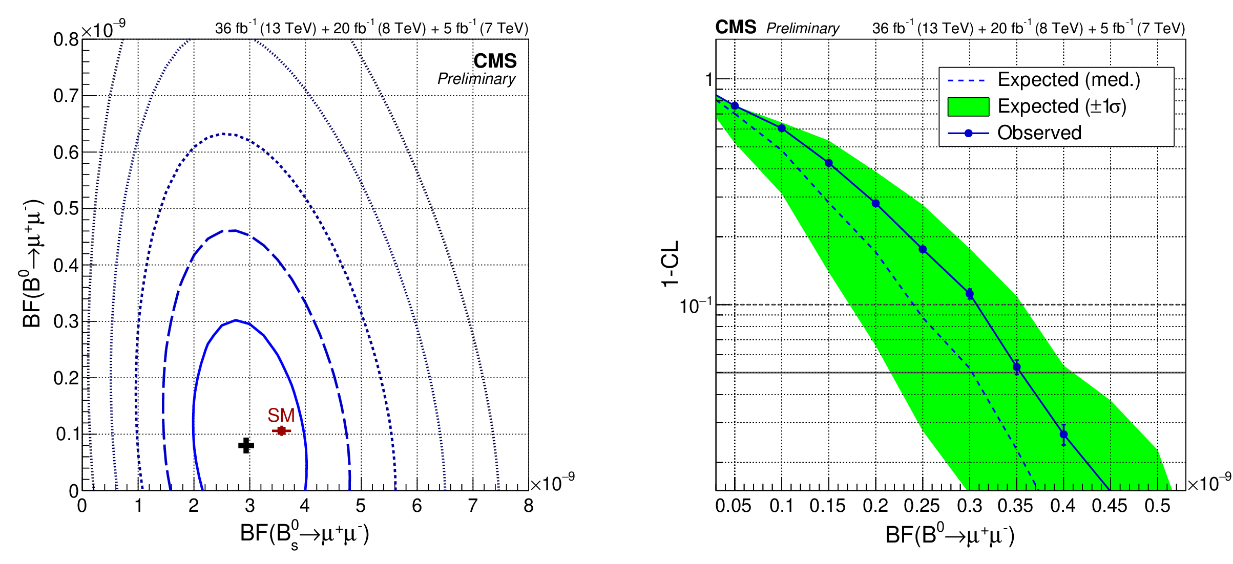
| Abstract: Results are reported for the ${\rm B_s^0}\to\mu^+\mu^-$ branching fraction and effective lifetime and from a search for the decay ${\rm B^0}\to\mu^+\mu^-$. The analysis uses a data sample of proton-proton collisions accumulated by the CMS experiment in 2011, 2012, and 2016, with center-of-mass energies (integrated luminosities) of 7 TeV (5 fb$^{-1}$), 8 TeV (20 fb$^{-1}$), and 13 TeV (36 fb$^{-1}$). The branching fractions are determined by measuring efficiency-corrected event yields relative to ${\rm B^+}\to{\rm J}/\psi {\rm K^+}$ decays (with ${\rm J}/\psi\to\mu^+\mu^-$), which results in the cancellation of many of the systematic uncertainties. The decay ${\rm B_s^0}\to\mu^+\mu^-$ is observed with a branching fraction of ${\cal B}({\rm B_s^0}\to\mu^+\mu^-) =$ [2.9$^{+0.7}_{-0.6}$ (exp) $\pm$ 0.2 (frag)] $\times10^{-9}$, where frag refers to the uncertainty in the ratio $f_s/f_u$ of the ${\rm B_s^0}$ and the ${\rm B^+}$ fragmentation functions, corresponding to a significance of 5.6 standard deviations. No significant excess is observed for the decay ${\rm B^0}\to\mu^+\mu^-$, and the upper limit ${\cal B}({\rm B^0}\to\mu^+\mu^-) < 3.6\times10^{-10}$ is obtained at 95% confidence level. These measured branching fractions are consistent with standard model predictions, and they supersede previous results from CMS based on the 2011 and 2012 data only. Finally, the ${\rm B_s^0}\to\mu^+\mu^-$ effective lifetime is measured, for the first time in CMS, and is found to be $\tau_{\mu^+\mu^-} = $ 1.70$^{+0.61}_{-0.44}$ ps. | ||
|
Links:
CDS record (PDF) ;
CADI line (restricted) ;
These preliminary results are superseded in this paper, JHEP 04 (2020) 188. The superseded preliminary plots can be found here. |
||
| Figures & Tables | Summary | Additional Figures | References | CMS Publications |
|---|
| Figures | |
png pdf |
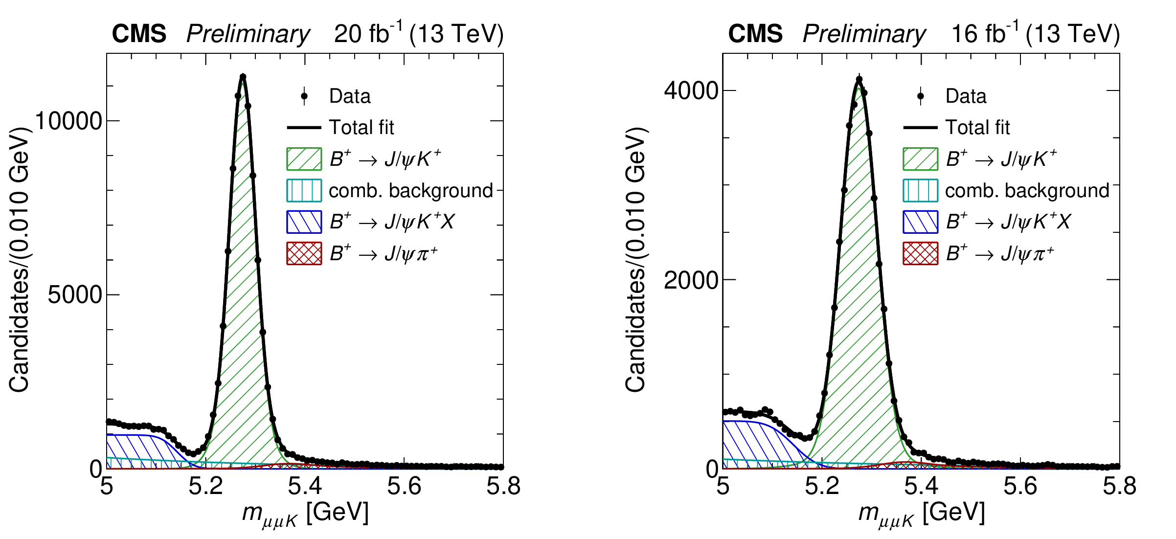
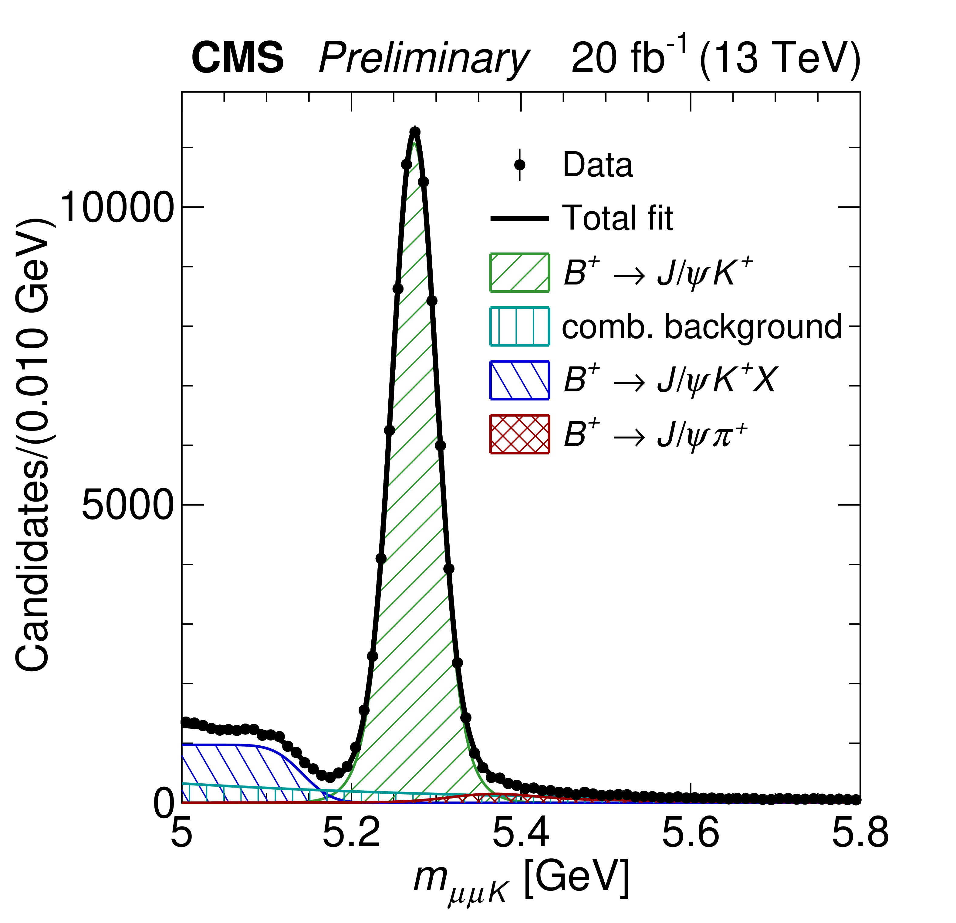
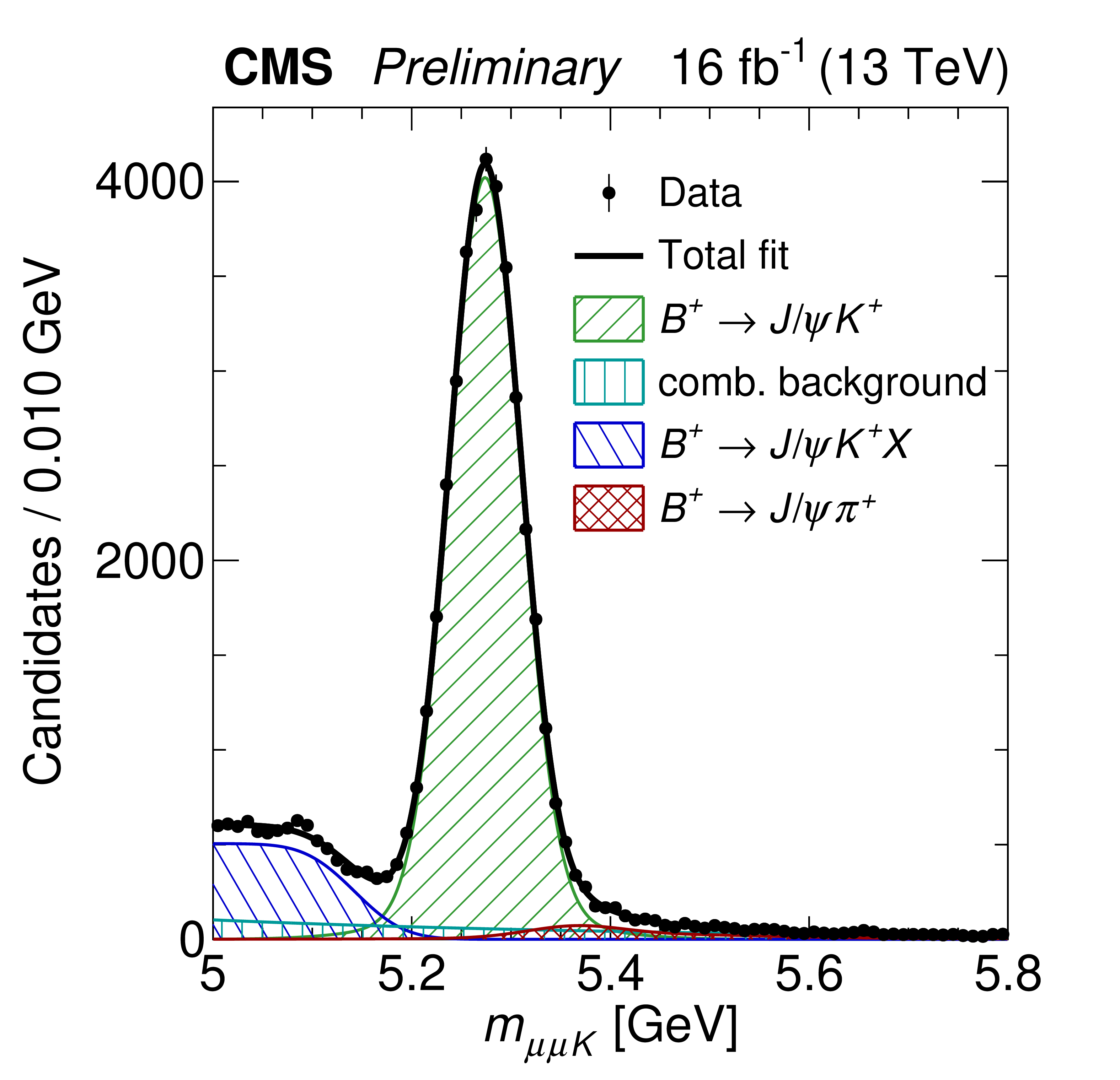
Figure 1:
Invariant-mass distributions for the $\mu \mu K$ system used to reconstruct the $ {\mathrm{B^{+}} \to {\mathrm{J}/\psi} \mathrm{K^{+}}} $ normalization sample. The plot on the left shows the 2016A central-region channel ($ {| {\eta ^{\text {f}}_{\mu}} |} < $ 0.7), while the plot on the right shows the 2016B forward-region channel (0.7 $ < {| {\eta ^{\text {f}}_{\mu}} |} < $ 1.4). The mass resolutions for these channels are 30 and 43 MeV, respectively. The data are shown by solid black circles, the result of the fit is overlayed with the black line, and the different components are indicated by the hatched regions. |
png pdf |
Figure 1-a:
Invariant-mass distributions for the $\mu \mu K$ system used to reconstruct the $ {\mathrm{B^{+}} \to {\mathrm{J}/\psi} \mathrm{K^{+}}} $ normalization sample. The plot on the left shows the 2016A central-region channel ($ {| {\eta ^{\text {f}}_{\mu}} |} < $ 0.7), while the plot on the right shows the 2016B forward-region channel (0.7 $ < {| {\eta ^{\text {f}}_{\mu}} |} < $ 1.4). The mass resolutions for these channels are 30 and 43 MeV, respectively. The data are shown by solid black circles, the result of the fit is overlayed with the black line, and the different components are indicated by the hatched regions. |

png pdf |
Figure 1-b:
Invariant-mass distributions for the $\mu \mu K$ system used to reconstruct the $ {\mathrm{B^{+}} \to {\mathrm{J}/\psi} \mathrm{K^{+}}} $ normalization sample. The plot on the left shows the 2016A central-region channel ($ {| {\eta ^{\text {f}}_{\mu}} |} < $ 0.7), while the plot on the right shows the 2016B forward-region channel (0.7 $ < {| {\eta ^{\text {f}}_{\mu}} |} < $ 1.4). The mass resolutions for these channels are 30 and 43 MeV, respectively. The data are shown by solid black circles, the result of the fit is overlayed with the black line, and the different components are indicated by the hatched regions. |
png pdf |
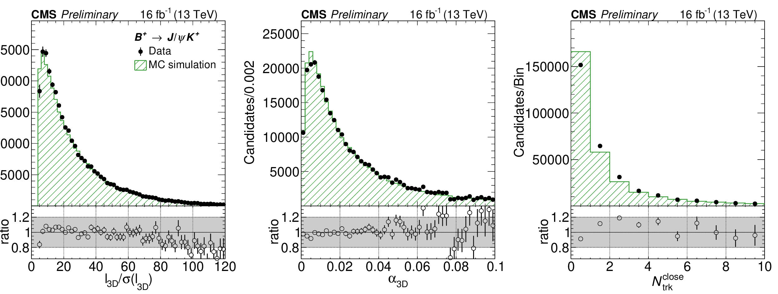
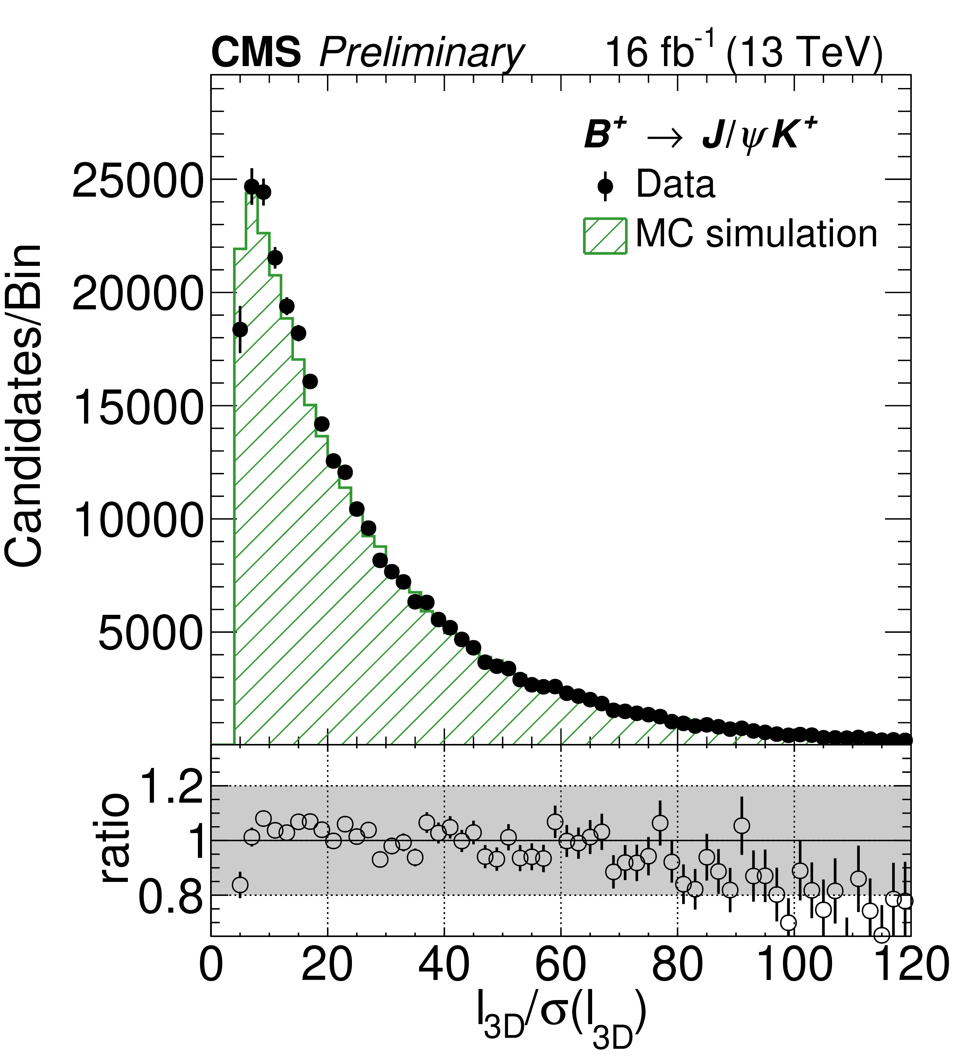
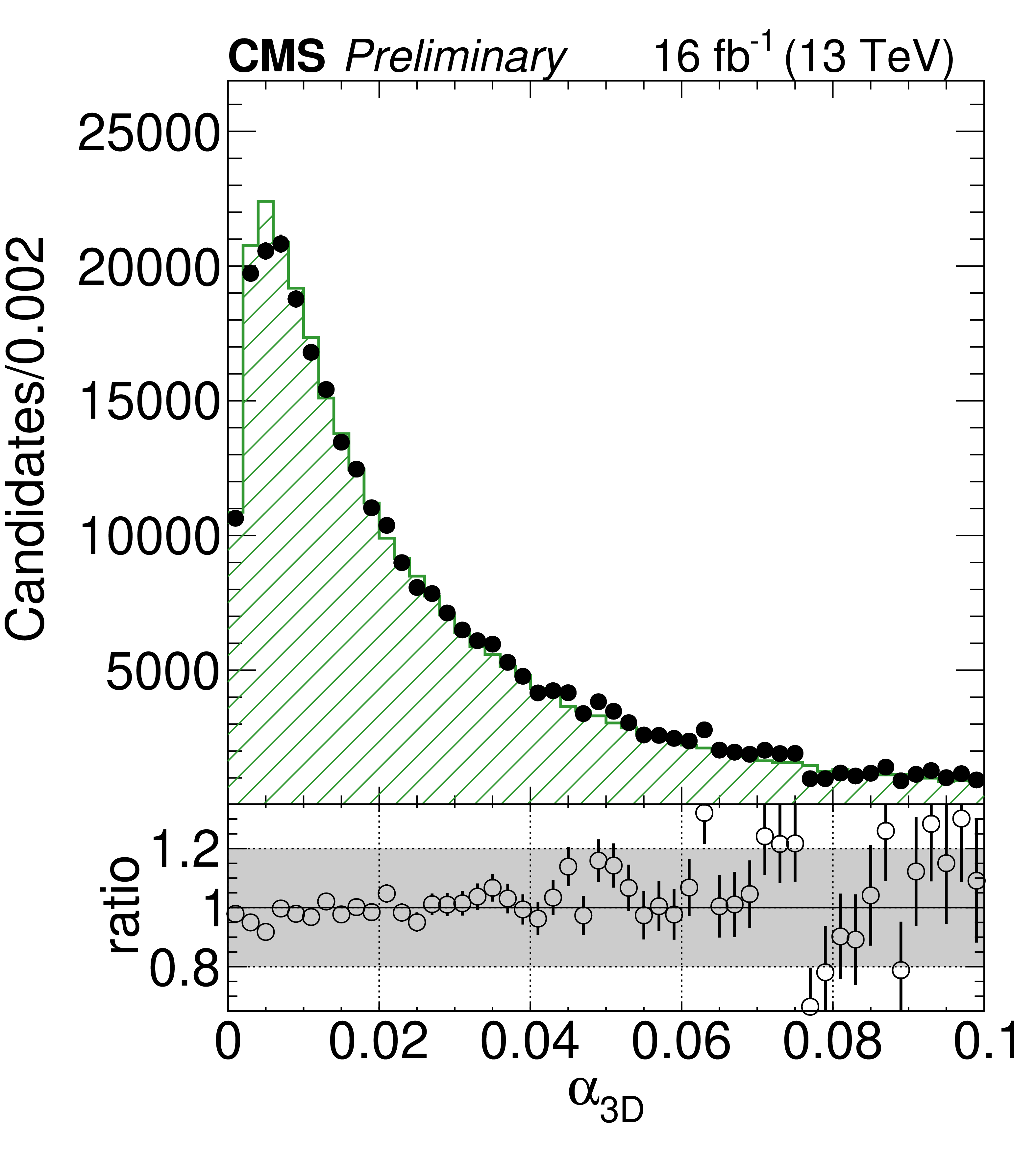
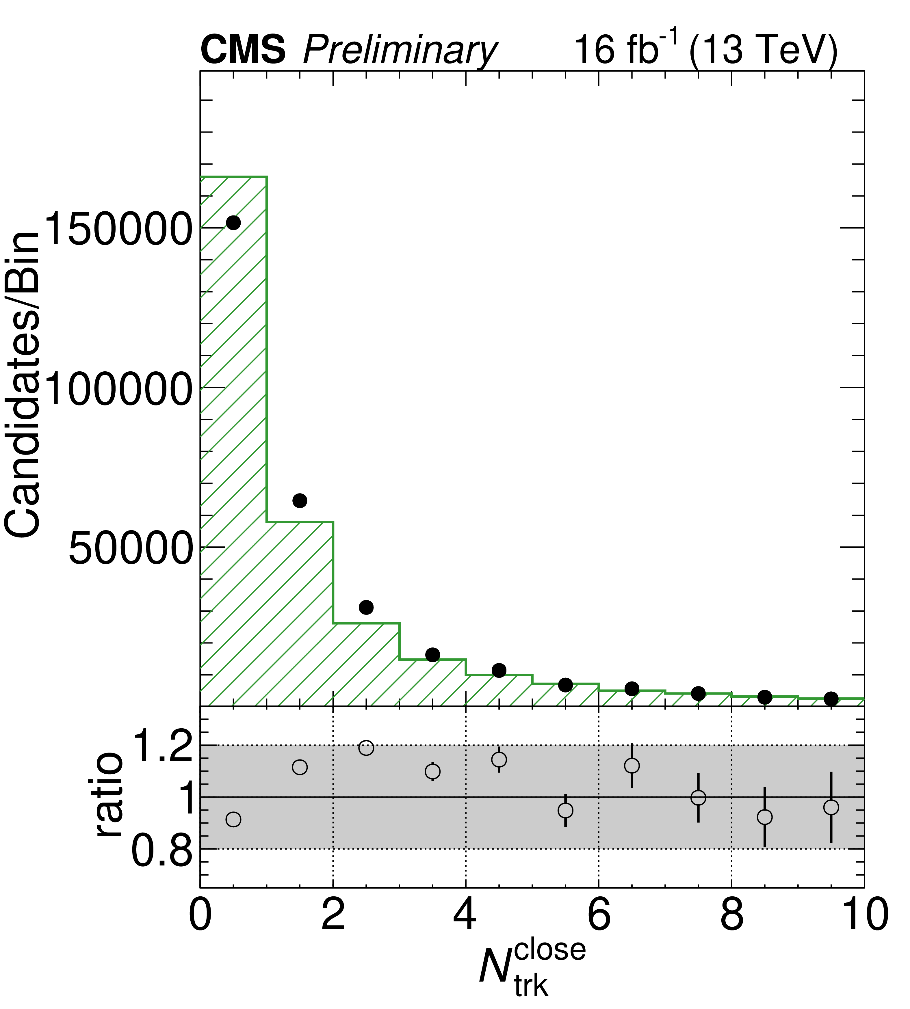
Figure 2:
Comparison of measured and simulated ${\mathrm{B^{+}} \to {\mathrm{J}/\psi} \mathrm{K^{+}}} $ distributions for the most discriminating analysis BDT variables in the central channel for 2016B: the flight length significance, the pointing angle, and the number of tracks close to the secondary vertex. The events are required to pass the preselection for the analysis BDT training. See text for details. The background-subtracted data are shown by solid circles and the MC simulation by the hatched histogram. The MC histograms are normalized to the number of events in the data. The band in the ratio plot shows the $ \pm $20% variation. |
png pdf |
Figure 2-a:
Comparison of measured and simulated ${\mathrm{B^{+}} \to {\mathrm{J}/\psi} \mathrm{K^{+}}} $ distributions for the most discriminating analysis BDT variables in the central channel for 2016B: the flight length significance, the pointing angle, and the number of tracks close to the secondary vertex. The events are required to pass the preselection for the analysis BDT training. See text for details. The background-subtracted data are shown by solid circles and the MC simulation by the hatched histogram. The MC histograms are normalized to the number of events in the data. The band in the ratio plot shows the $ \pm $20% variation. |
png pdf |
Figure 2-b:
Comparison of measured and simulated ${\mathrm{B^{+}} \to {\mathrm{J}/\psi} \mathrm{K^{+}}} $ distributions for the most discriminating analysis BDT variables in the central channel for 2016B: the flight length significance, the pointing angle, and the number of tracks close to the secondary vertex. The events are required to pass the preselection for the analysis BDT training. See text for details. The background-subtracted data are shown by solid circles and the MC simulation by the hatched histogram. The MC histograms are normalized to the number of events in the data. The band in the ratio plot shows the $ \pm $20% variation. |
png pdf |
Figure 2-c:
Comparison of measured and simulated ${\mathrm{B^{+}} \to {\mathrm{J}/\psi} \mathrm{K^{+}}} $ distributions for the most discriminating analysis BDT variables in the central channel for 2016B: the flight length significance, the pointing angle, and the number of tracks close to the secondary vertex. The events are required to pass the preselection for the analysis BDT training. See text for details. The background-subtracted data are shown by solid circles and the MC simulation by the hatched histogram. The MC histograms are normalized to the number of events in the data. The band in the ratio plot shows the $ \pm $20% variation. |
png pdf |
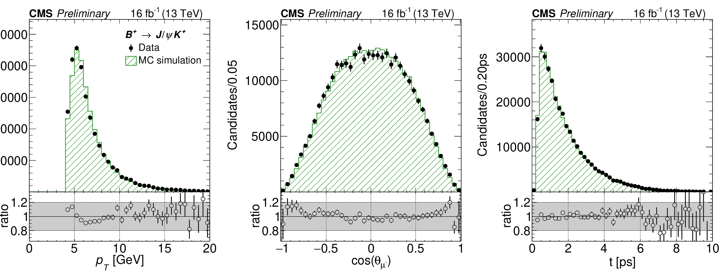
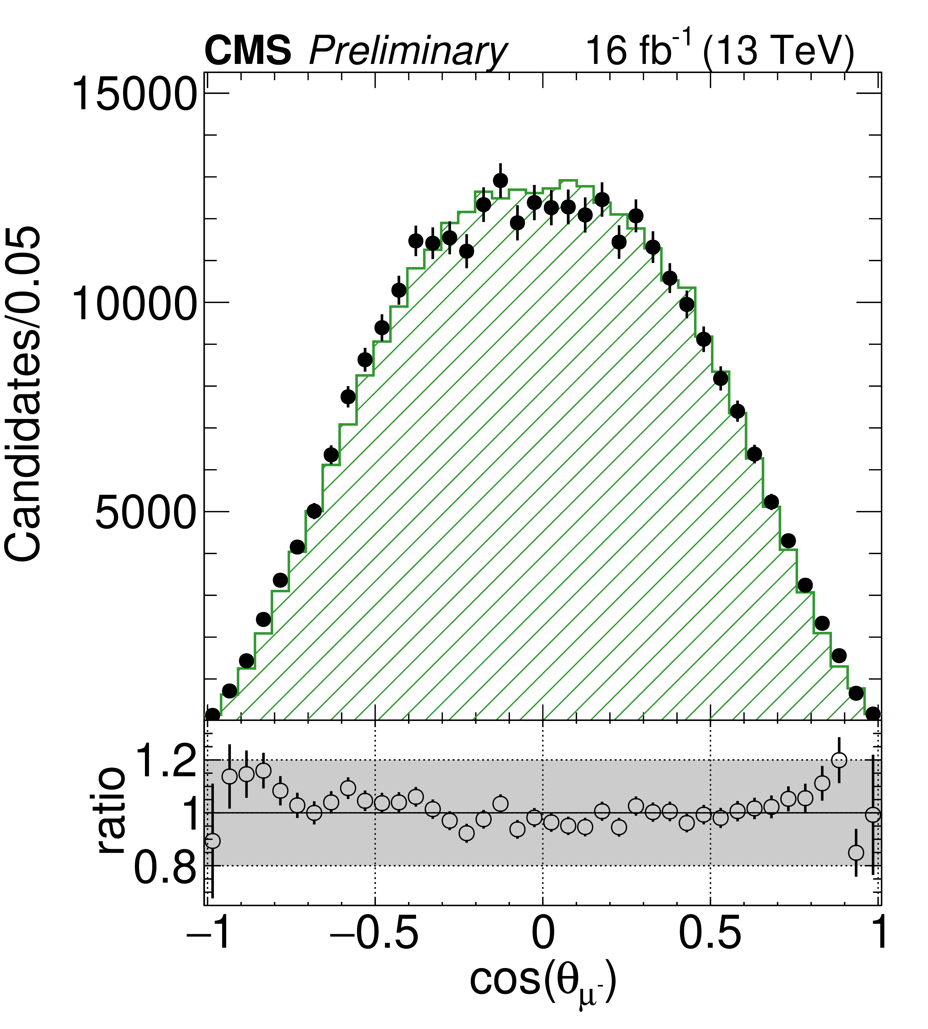
Figure 3:
Comparison of measured and simulated ${\mathrm{B^{+}} \to {\mathrm{J}/\psi} \mathrm{K^{+}}} $ distributions for kinematic variables in the central channel for 2016B: the subleading muon ${{p_{\text {T}}}}$, the muon helicity angle, and the B meson proper decay time. The events are required to pass the preselection for the analysis BDT training. See text for details. The background-subtracted data are shown by solid circles and the MC simulation by the hatched histogram. The MC histograms are normalized to the number of events in the data. The band in the ratio plot shows the $ \pm $20% variation. |

png pdf |
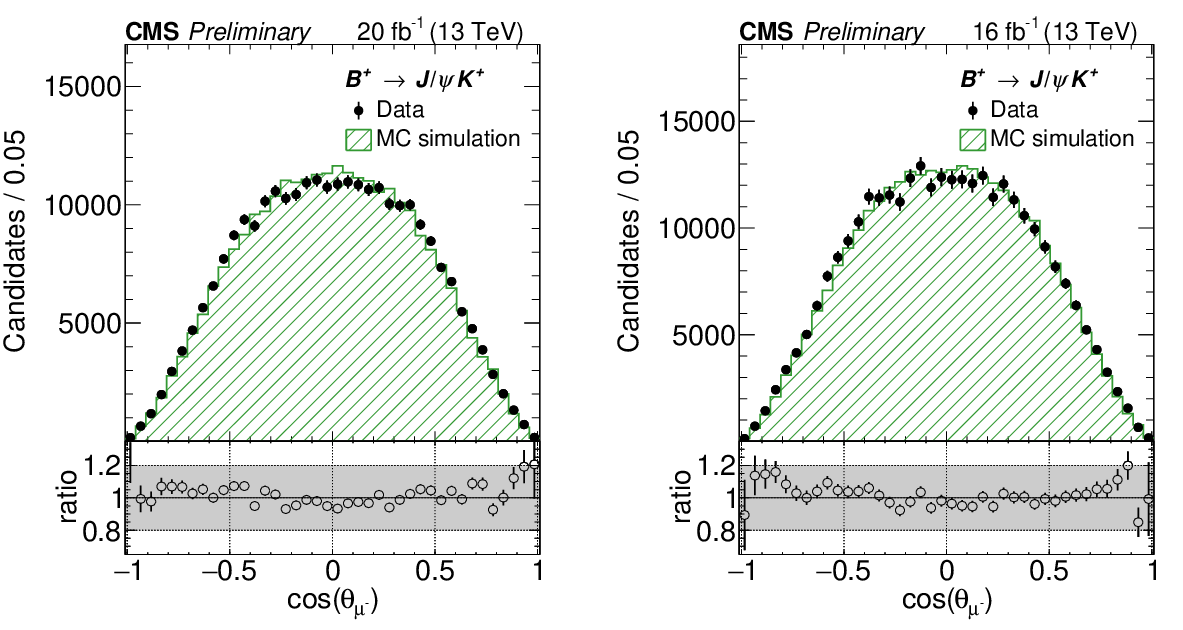
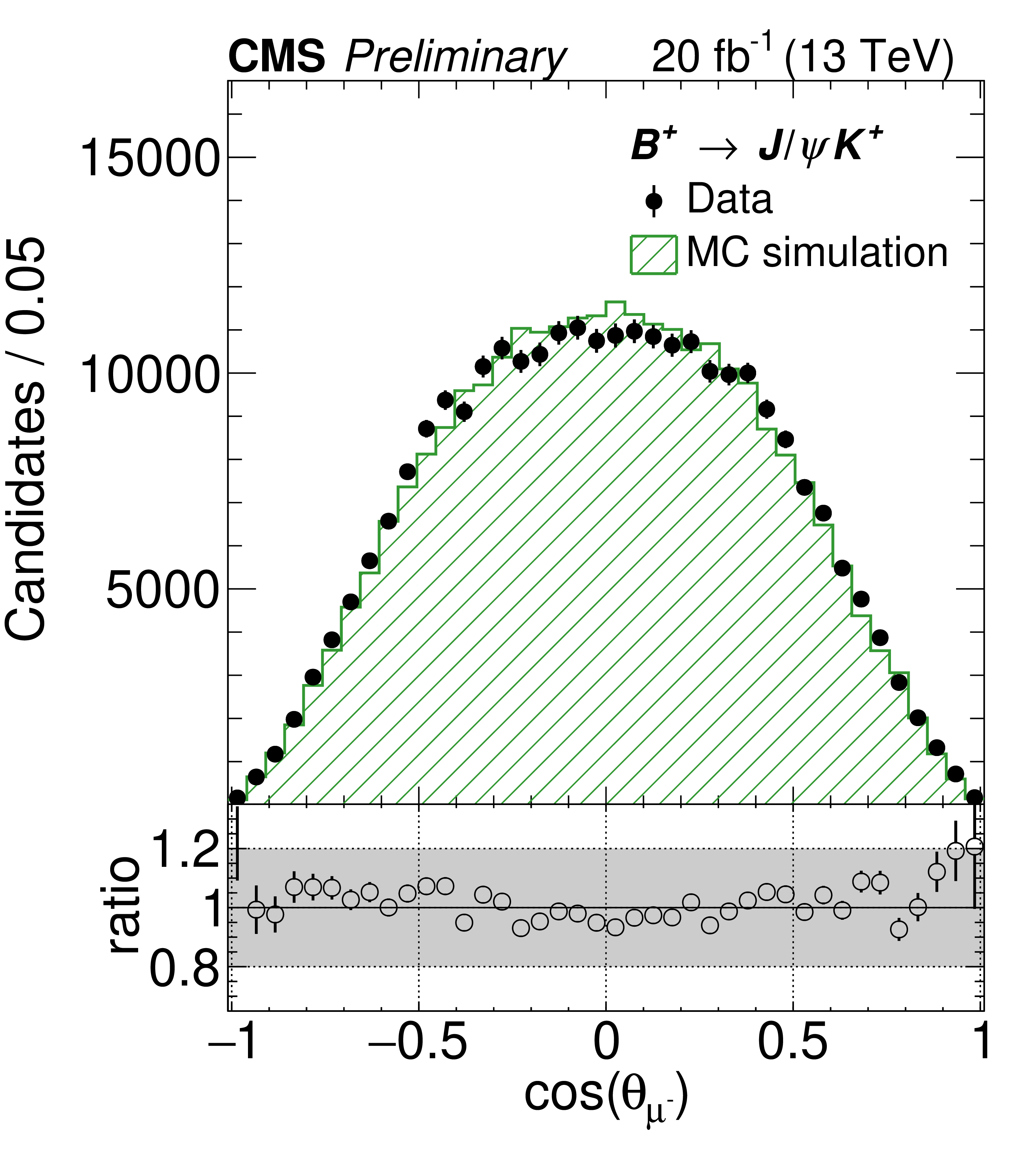
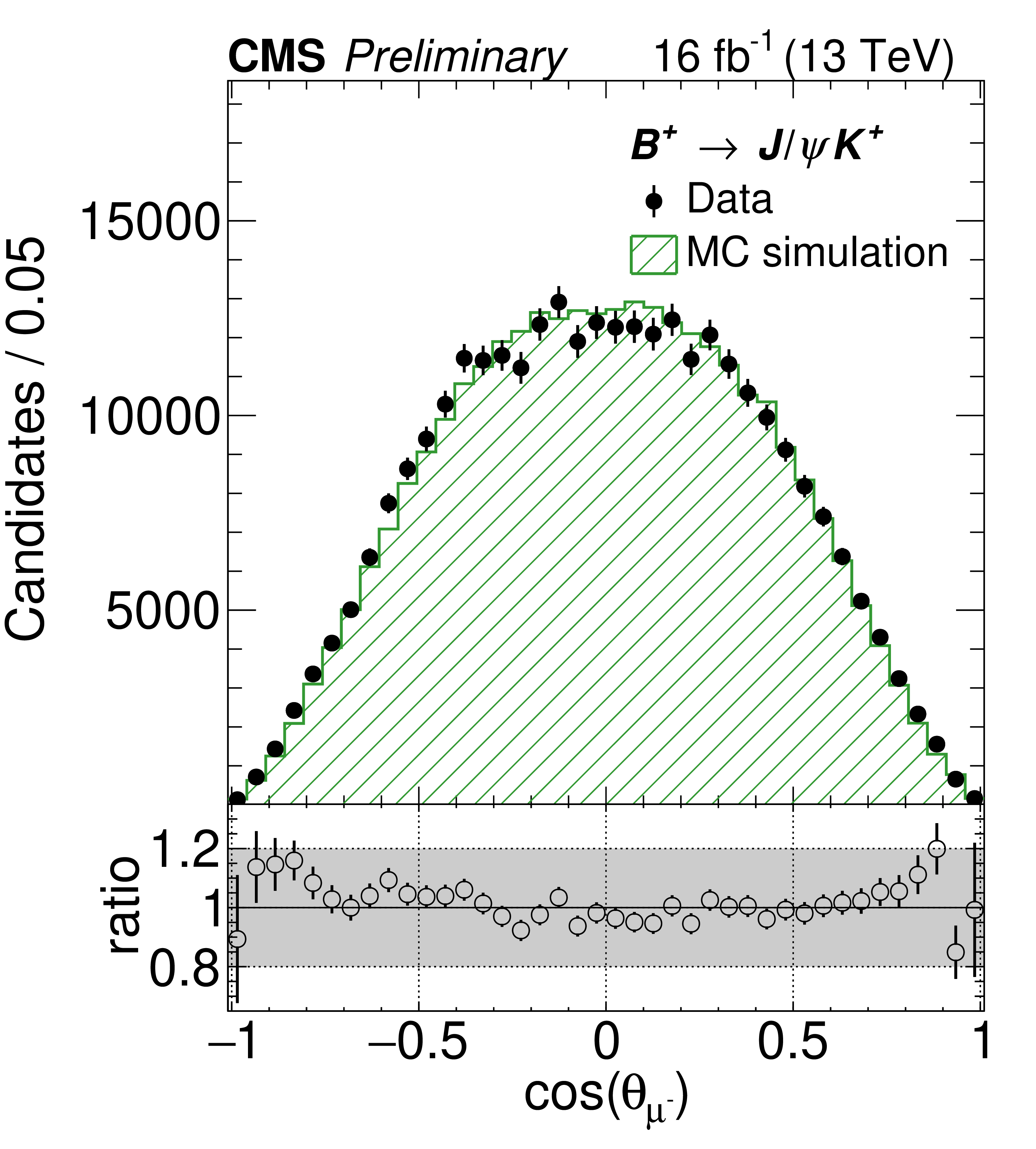
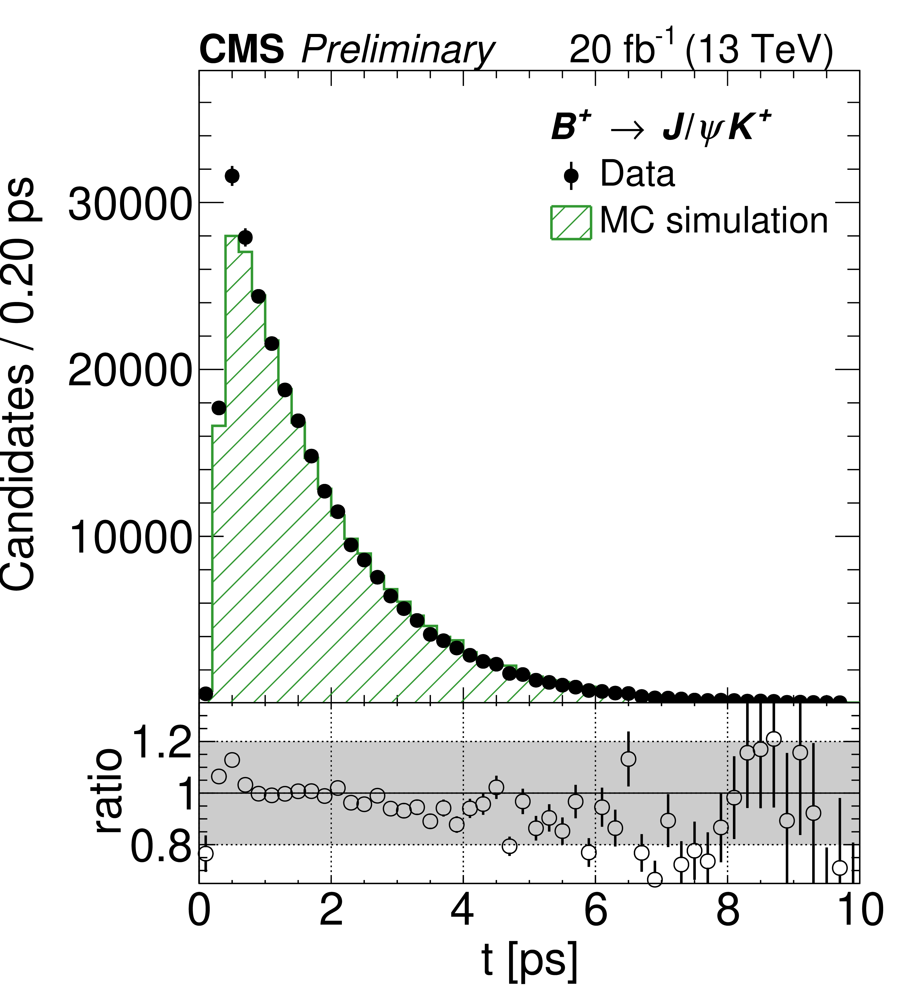
Figure 3-a:
Comparison of measured and simulated ${\mathrm{B^{+}} \to {\mathrm{J}/\psi} \mathrm{K^{+}}} $ distributions for kinematic variables in the central channel for 2016B: the subleading muon ${{p_{\text {T}}}}$, the muon helicity angle, and the B meson proper decay time. The events are required to pass the preselection for the analysis BDT training. See text for details. The background-subtracted data are shown by solid circles and the MC simulation by the hatched histogram. The MC histograms are normalized to the number of events in the data. The band in the ratio plot shows the $ \pm $20% variation. |
png pdf |
Figure 3-b:
Comparison of measured and simulated ${\mathrm{B^{+}} \to {\mathrm{J}/\psi} \mathrm{K^{+}}} $ distributions for kinematic variables in the central channel for 2016B: the subleading muon ${{p_{\text {T}}}}$, the muon helicity angle, and the B meson proper decay time. The events are required to pass the preselection for the analysis BDT training. See text for details. The background-subtracted data are shown by solid circles and the MC simulation by the hatched histogram. The MC histograms are normalized to the number of events in the data. The band in the ratio plot shows the $ \pm $20% variation. |
png pdf |
Figure 3-c:
Comparison of measured and simulated ${\mathrm{B^{+}} \to {\mathrm{J}/\psi} \mathrm{K^{+}}} $ distributions for kinematic variables in the central channel for 2016B: the subleading muon ${{p_{\text {T}}}}$, the muon helicity angle, and the B meson proper decay time. The events are required to pass the preselection for the analysis BDT training. See text for details. The background-subtracted data are shown by solid circles and the MC simulation by the hatched histogram. The MC histograms are normalized to the number of events in the data. The band in the ratio plot shows the $ \pm $20% variation. |
png pdf |
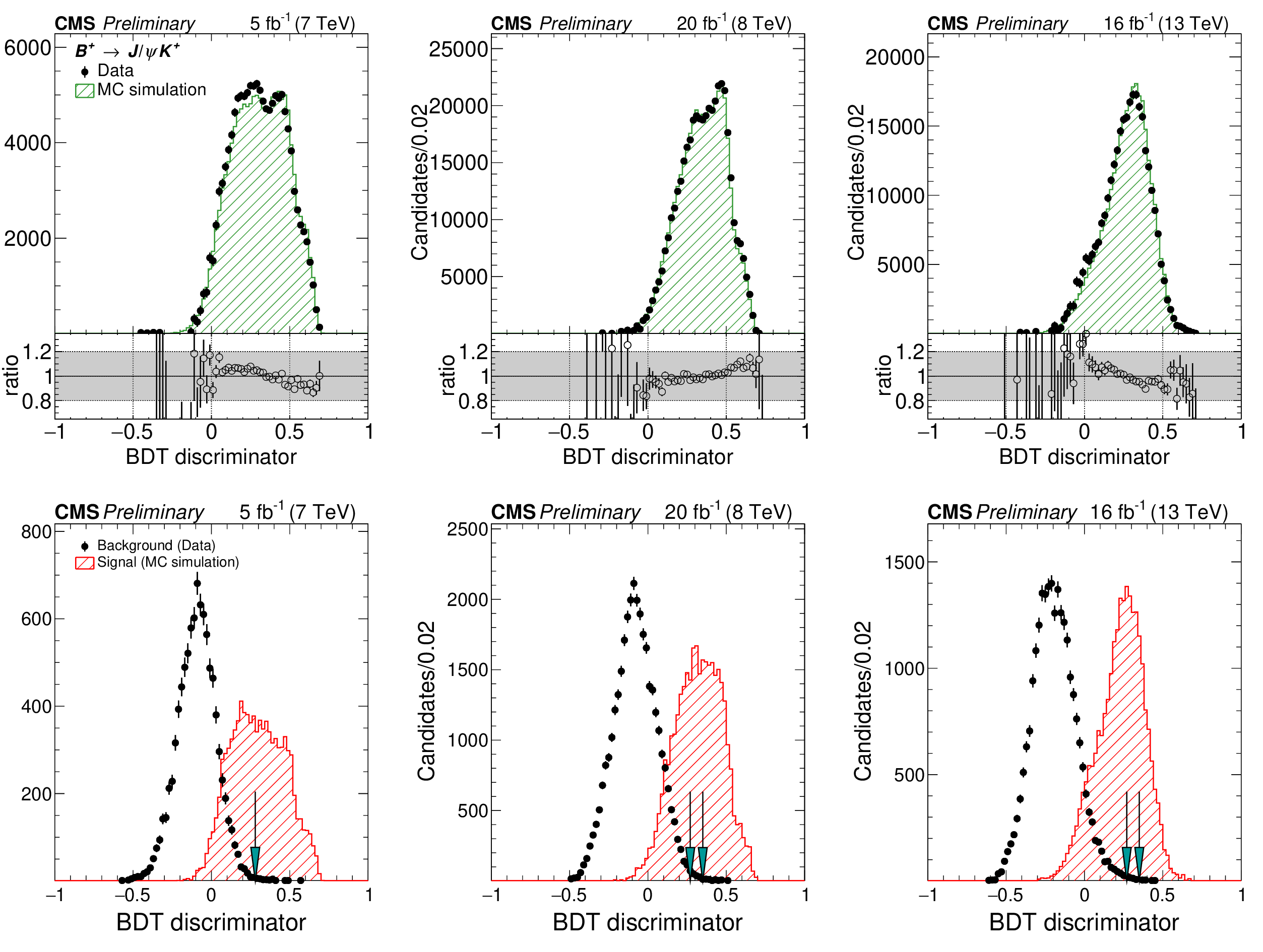
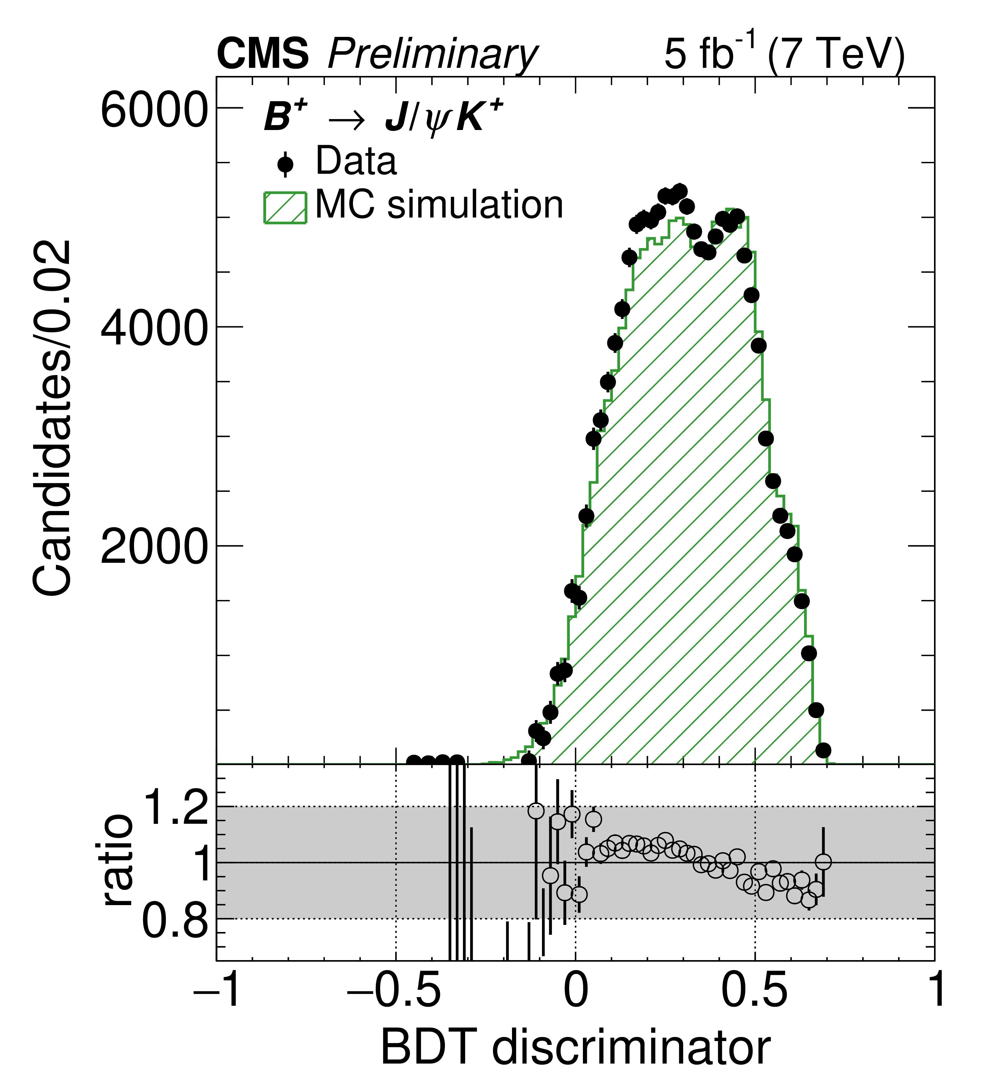
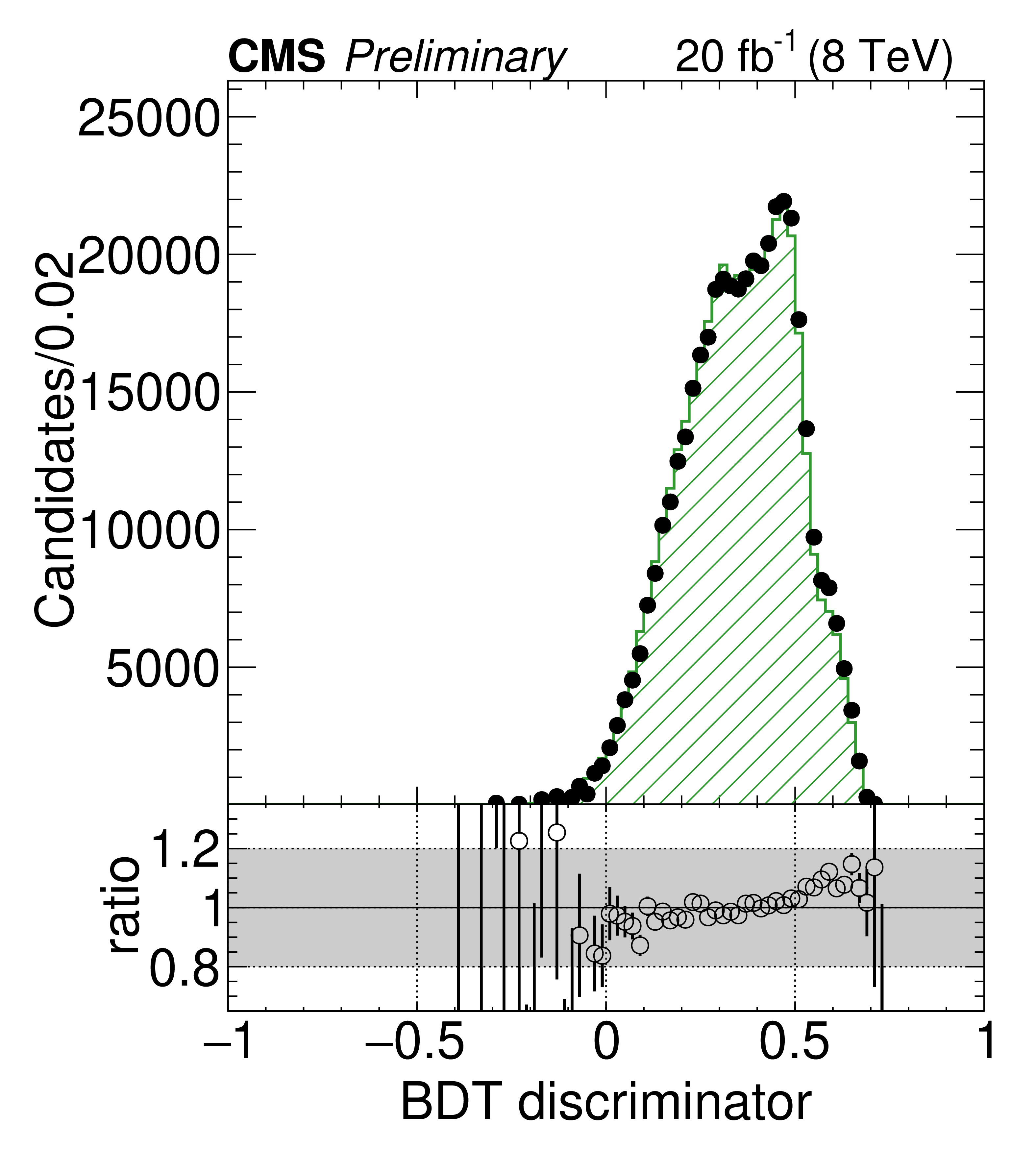
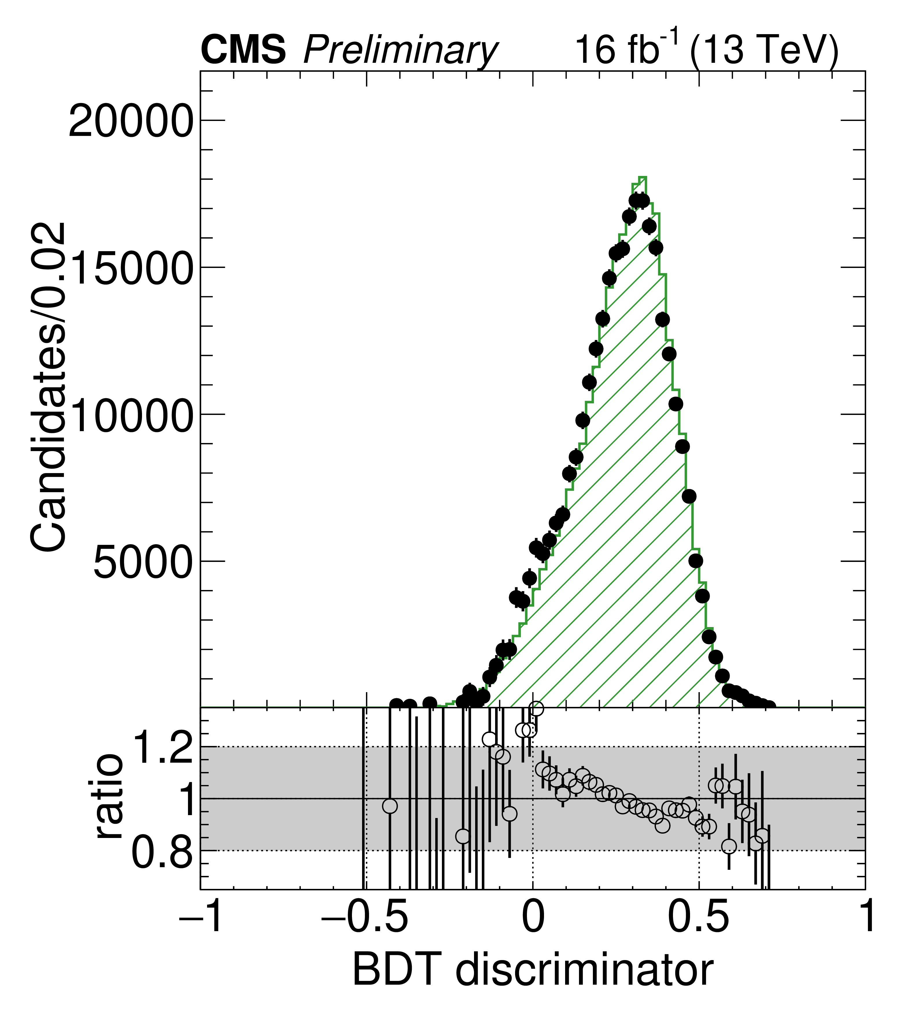
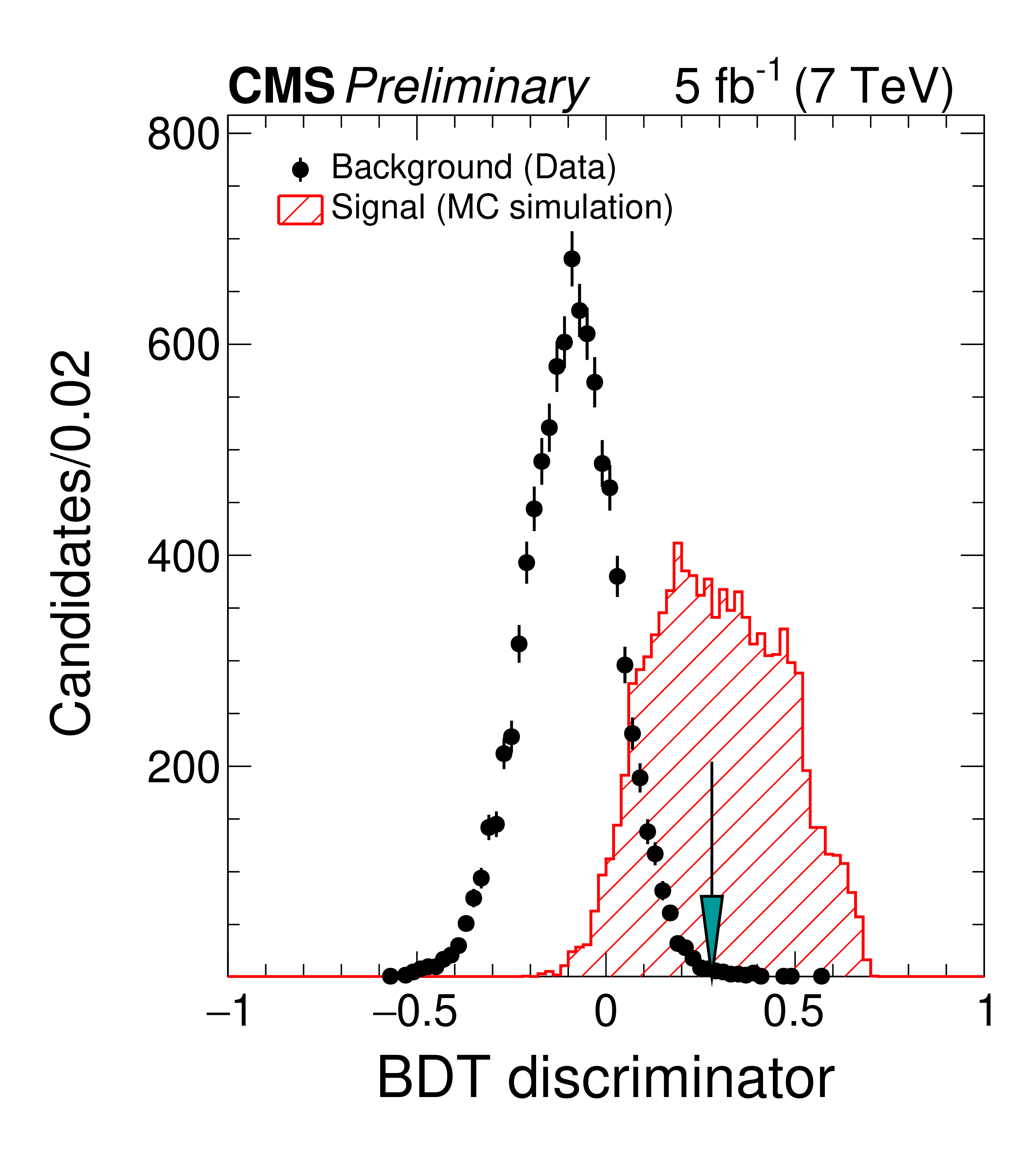
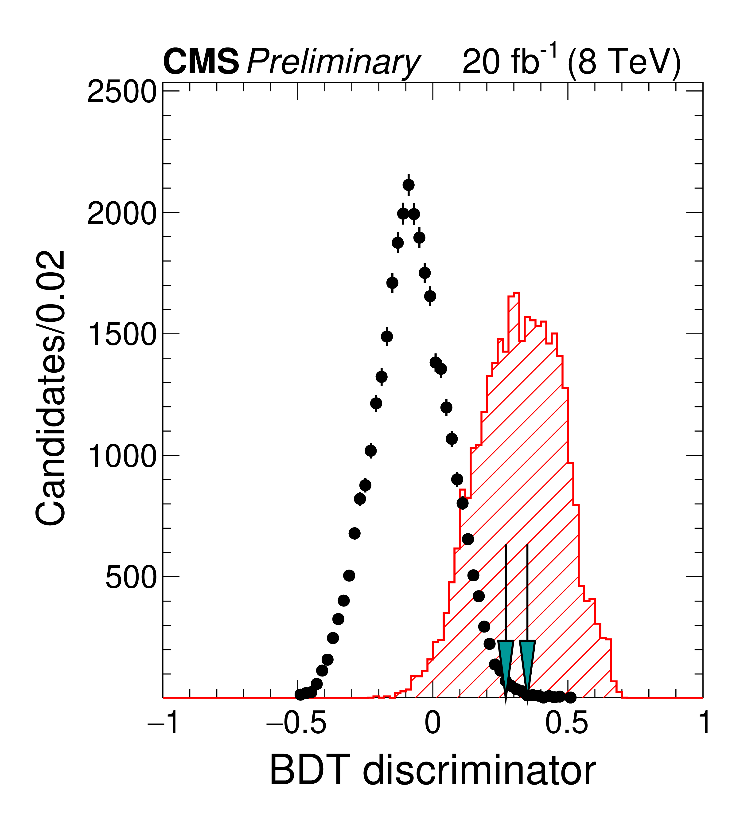
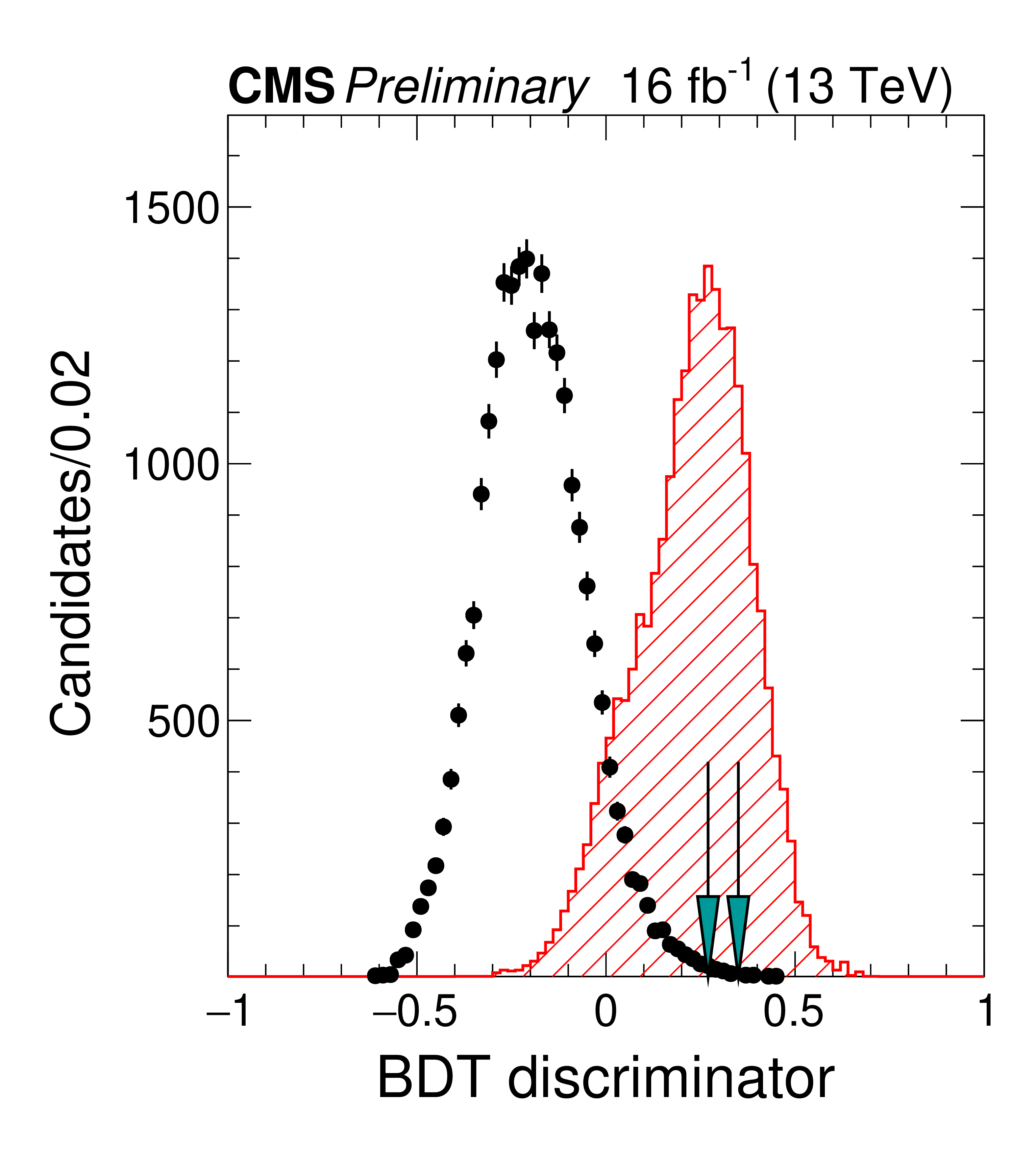
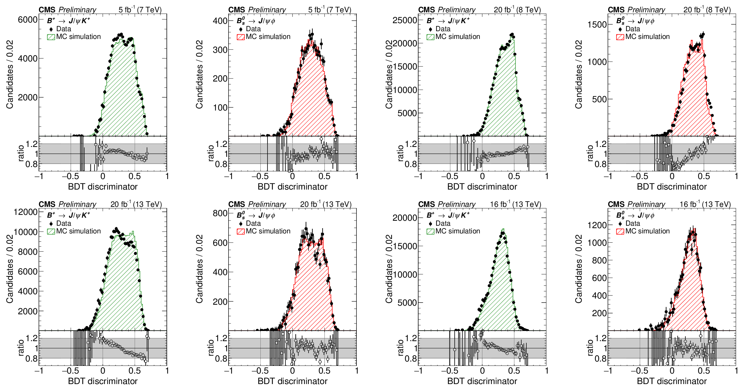
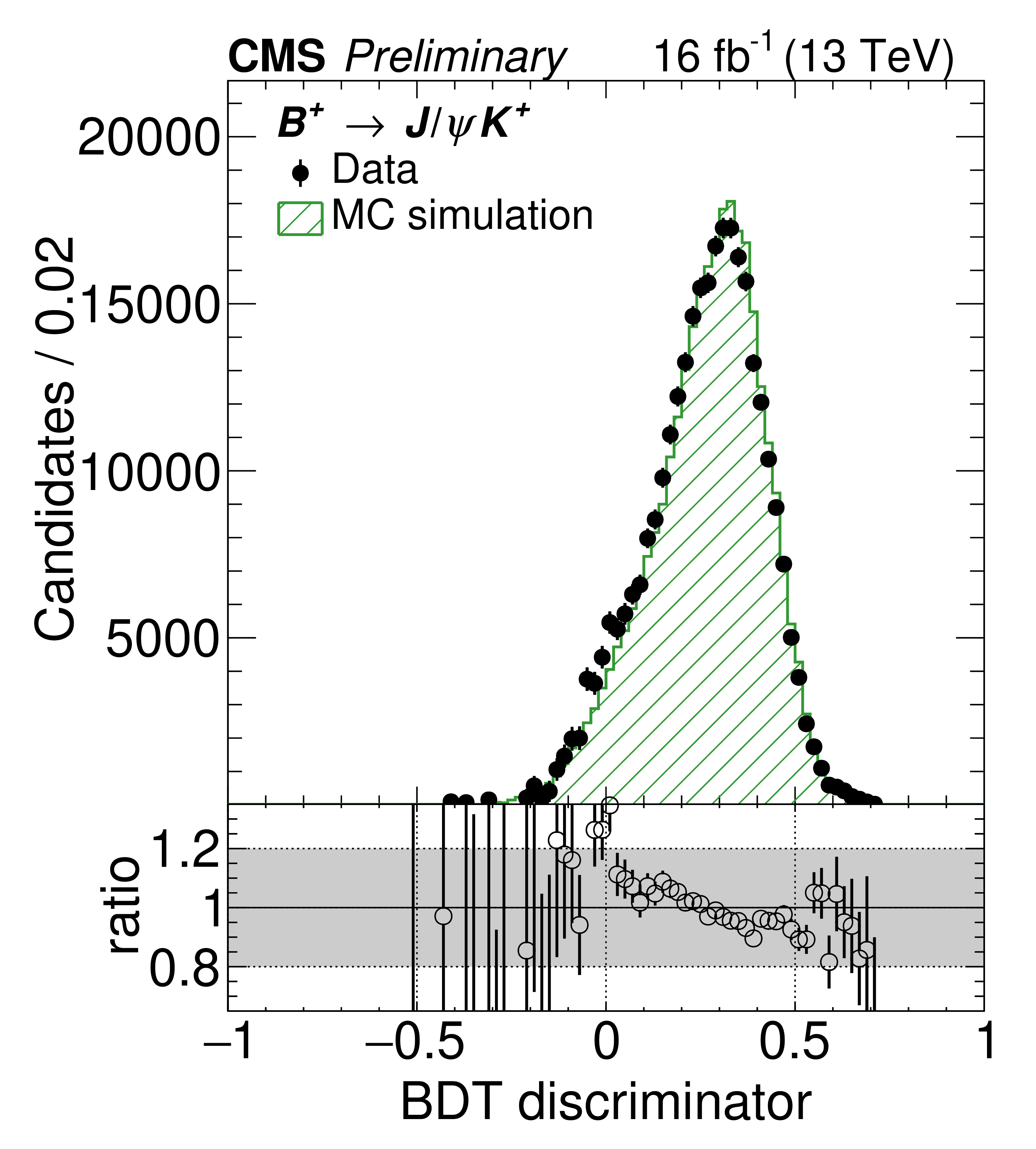
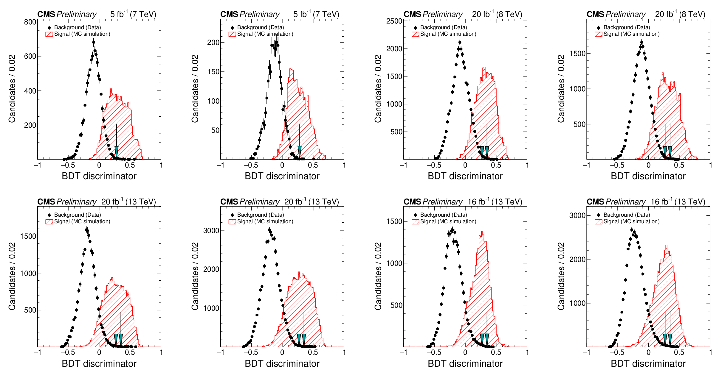
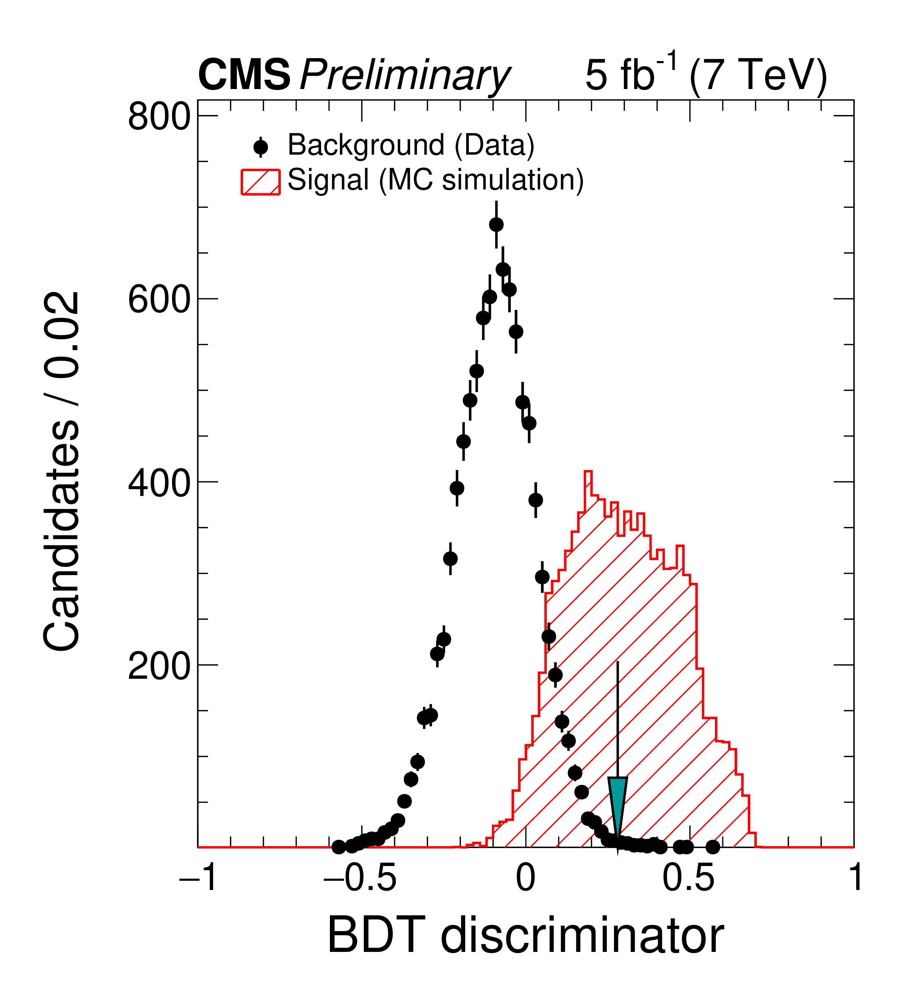
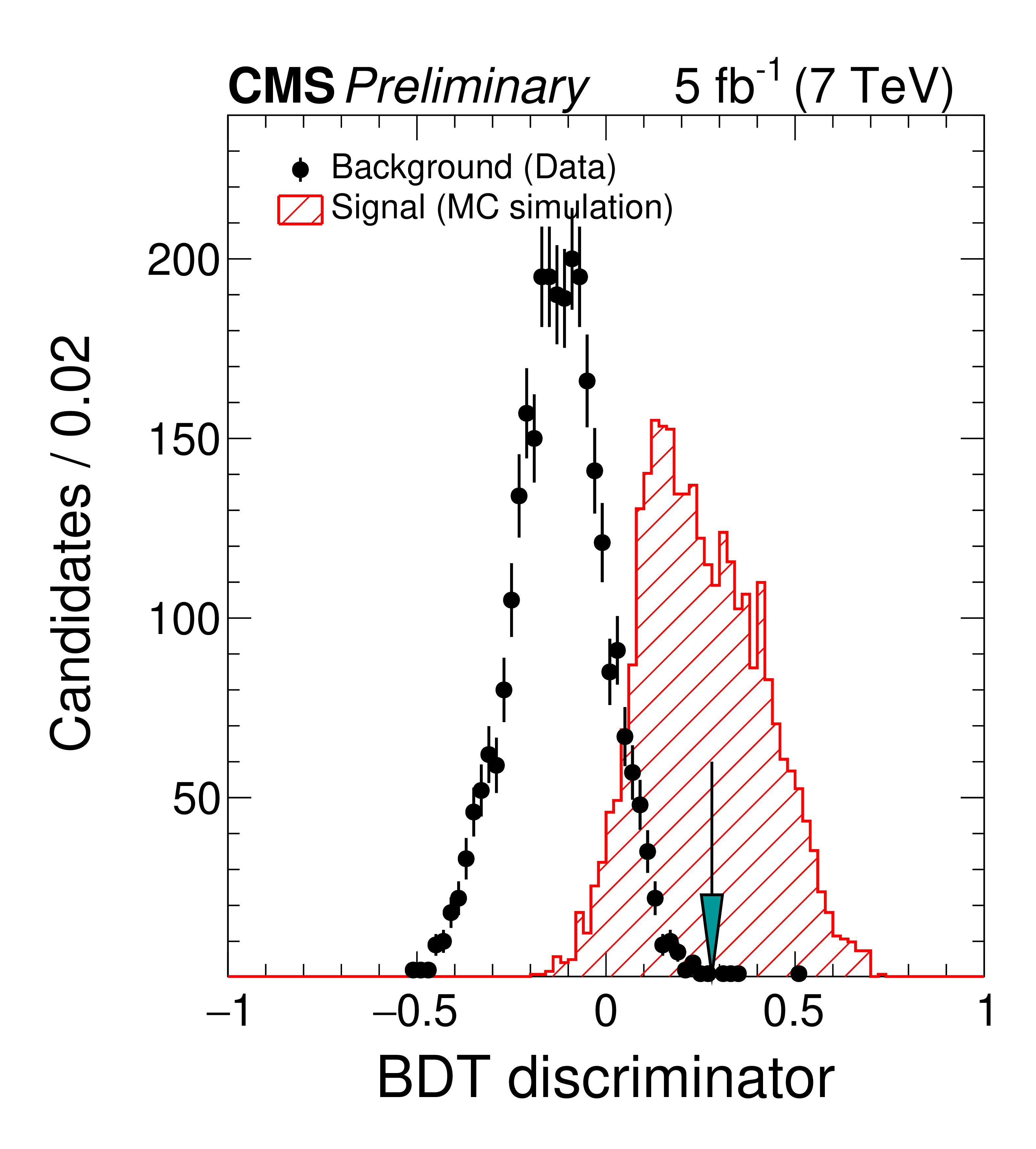
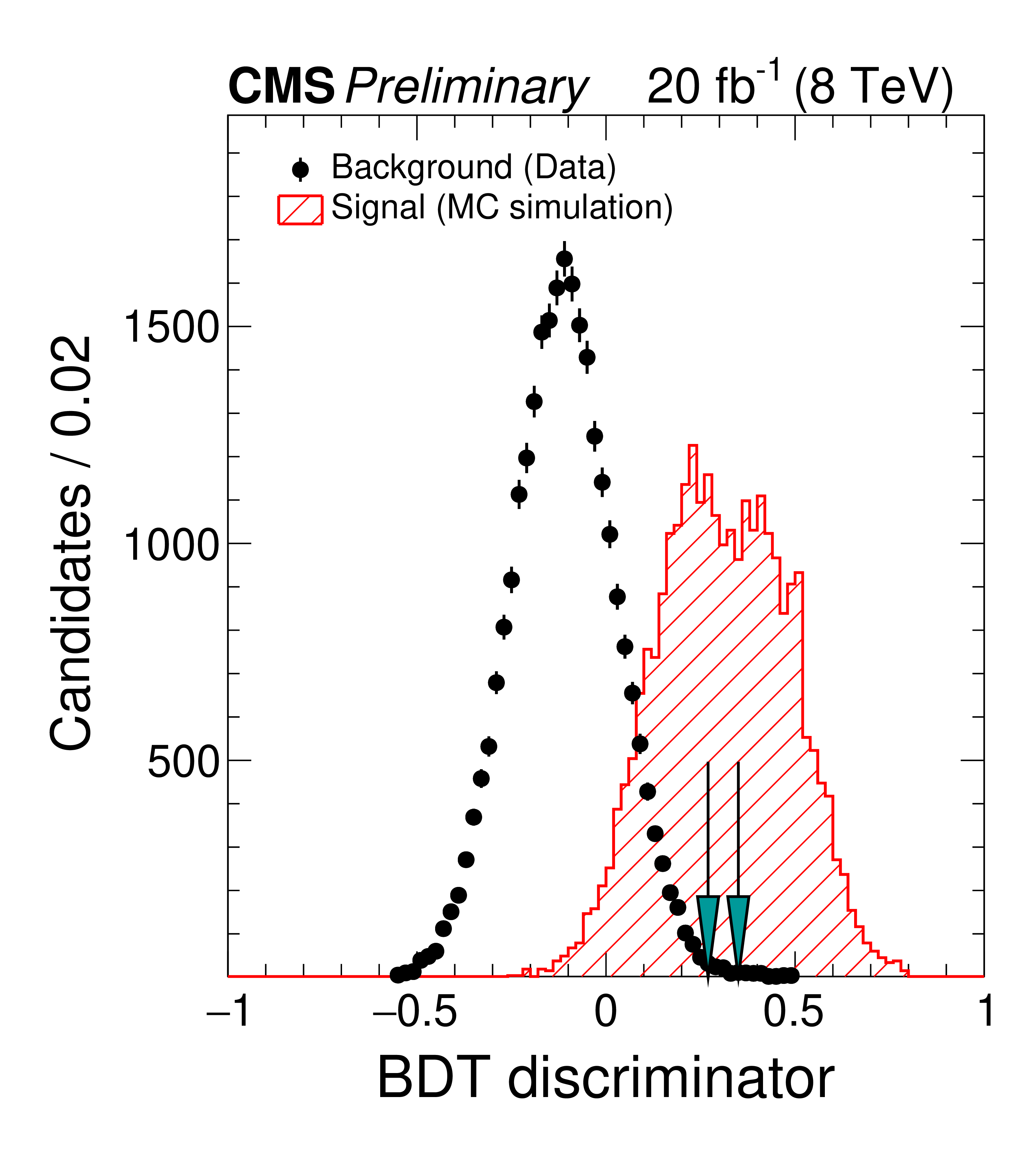
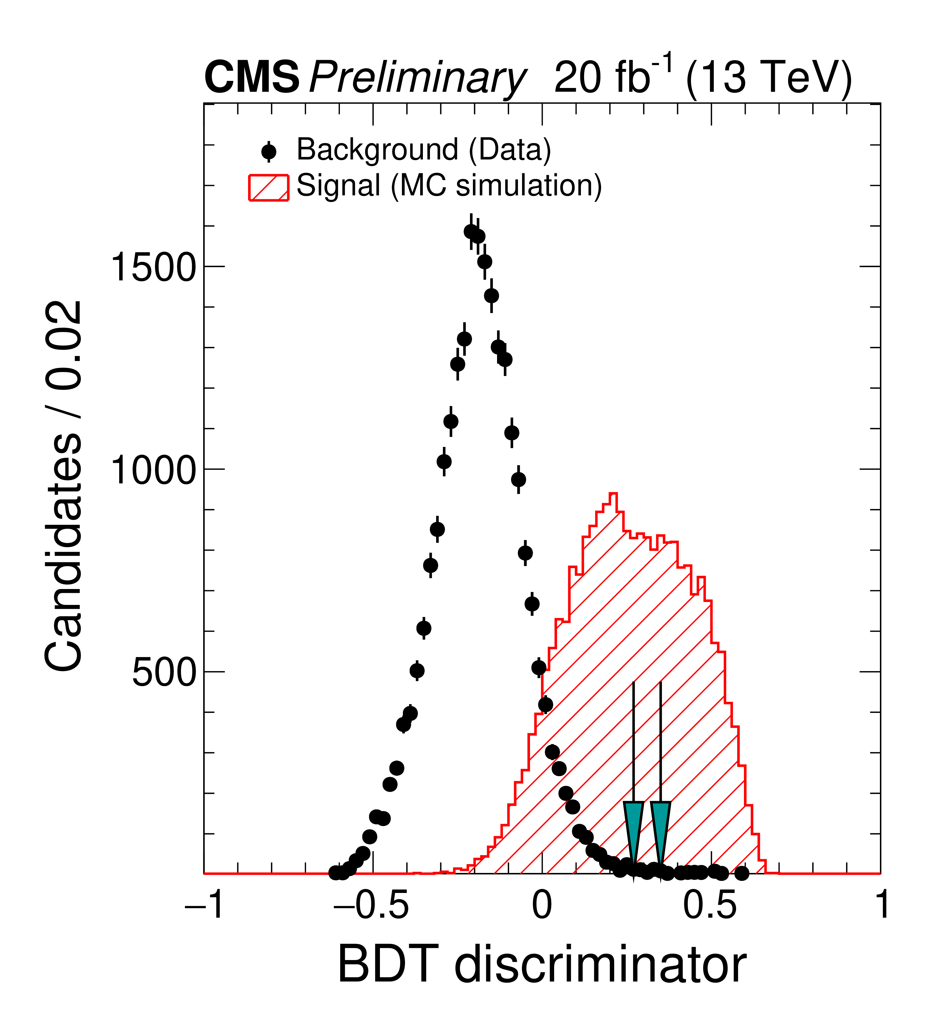
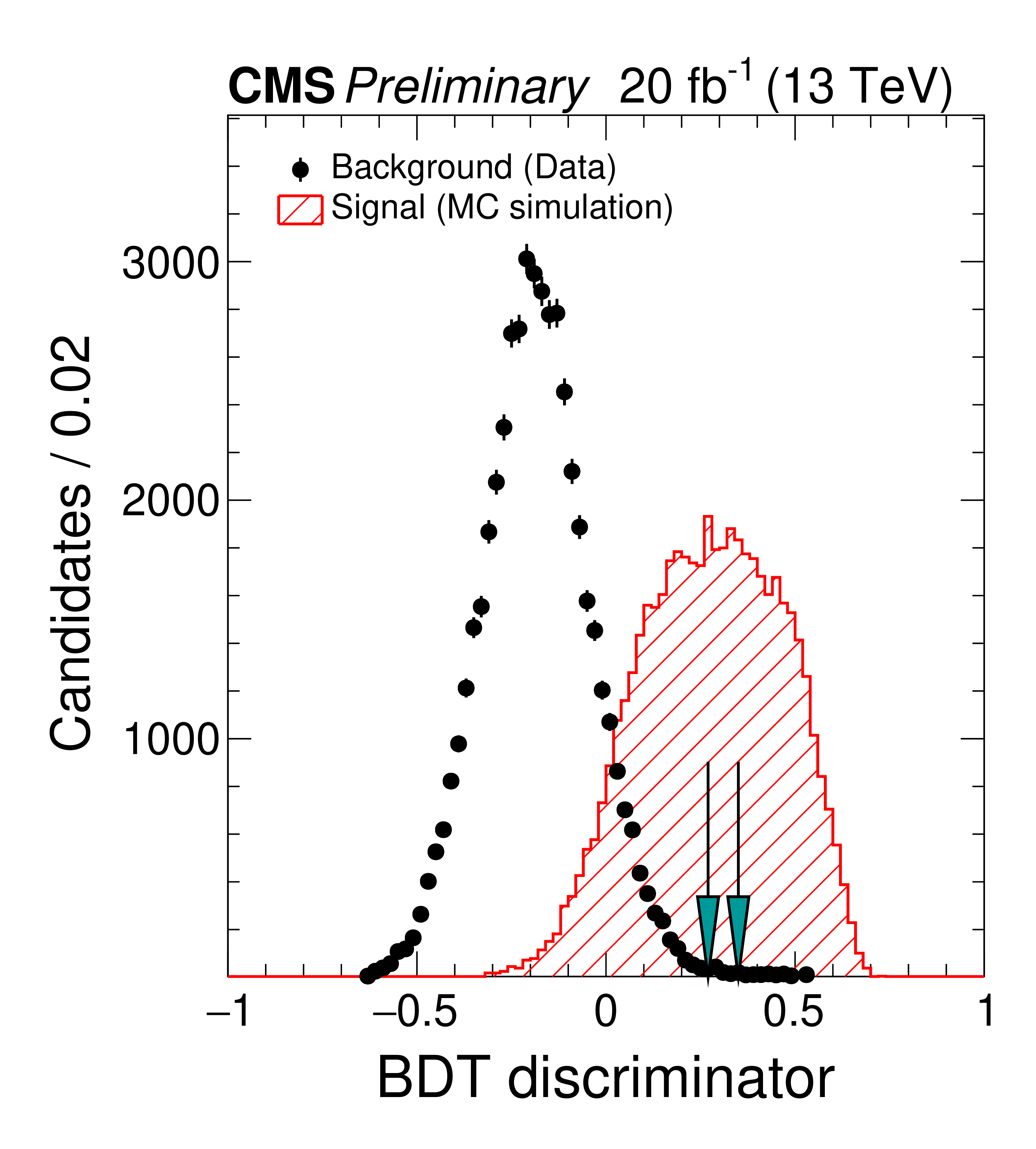
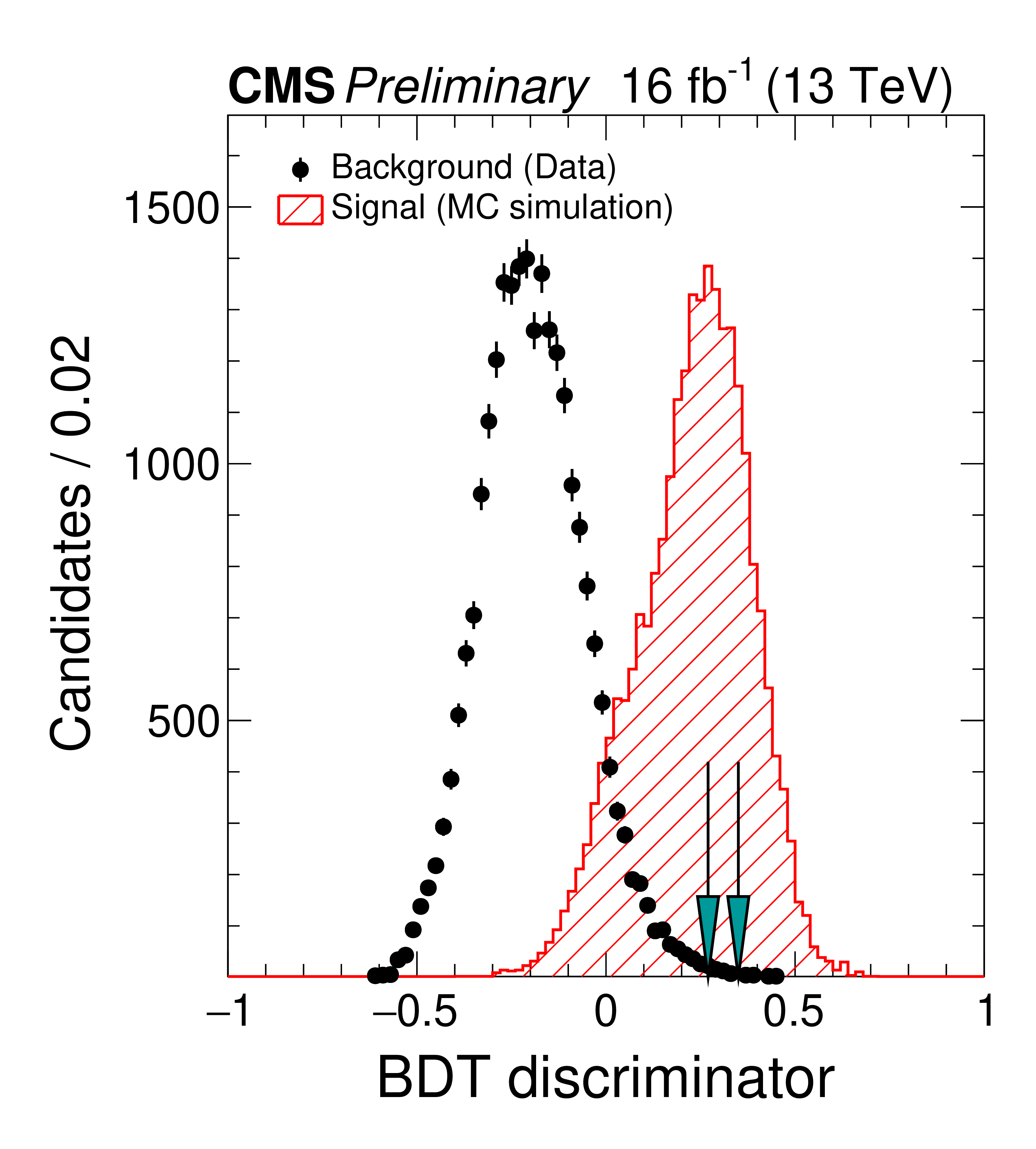
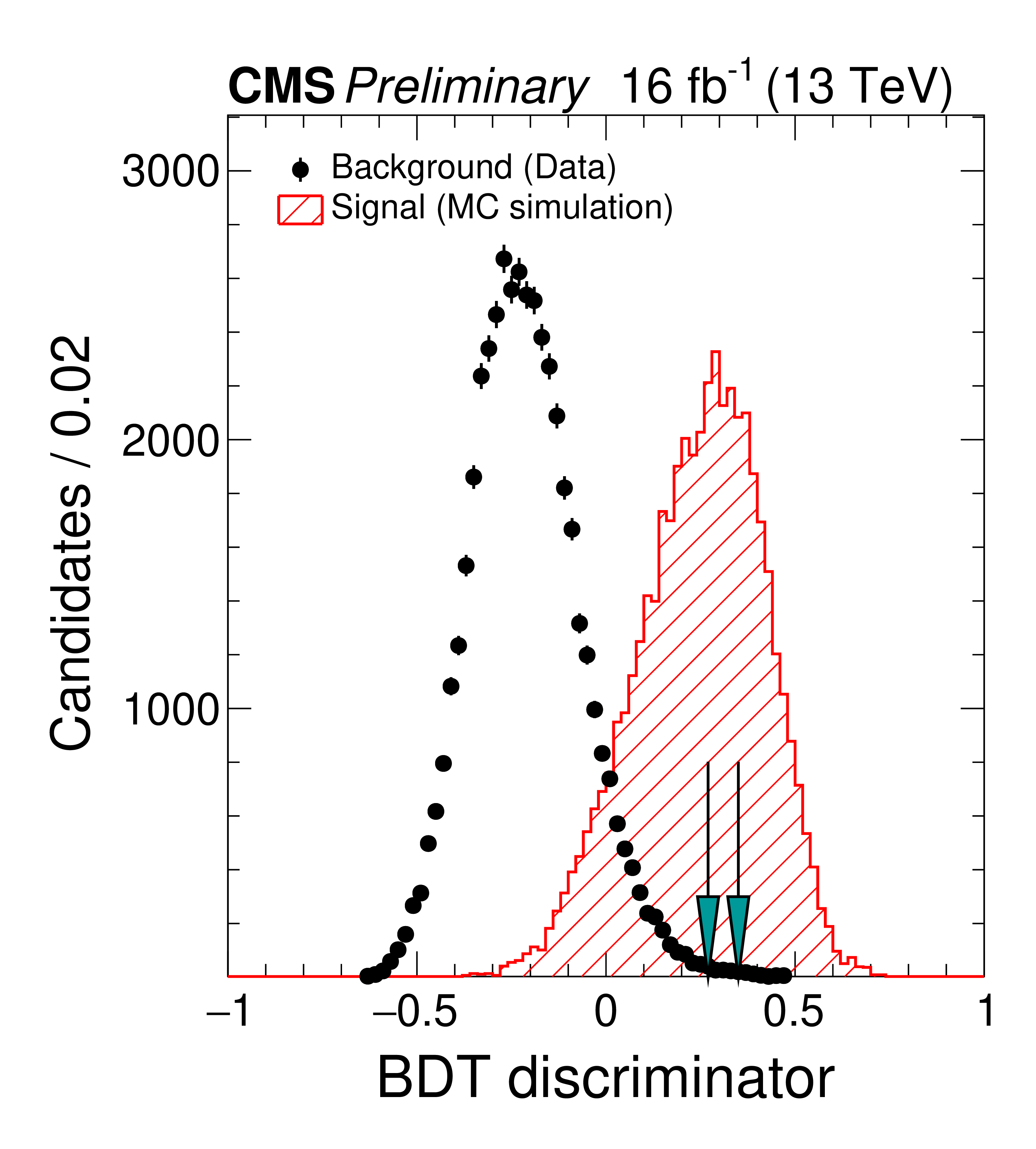
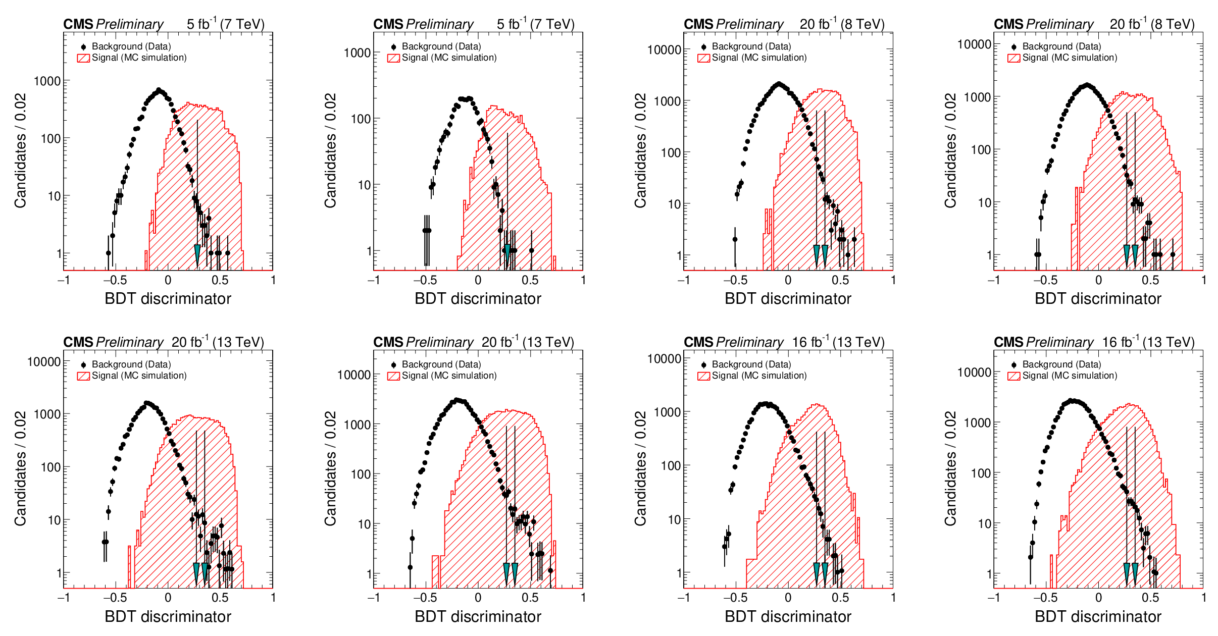
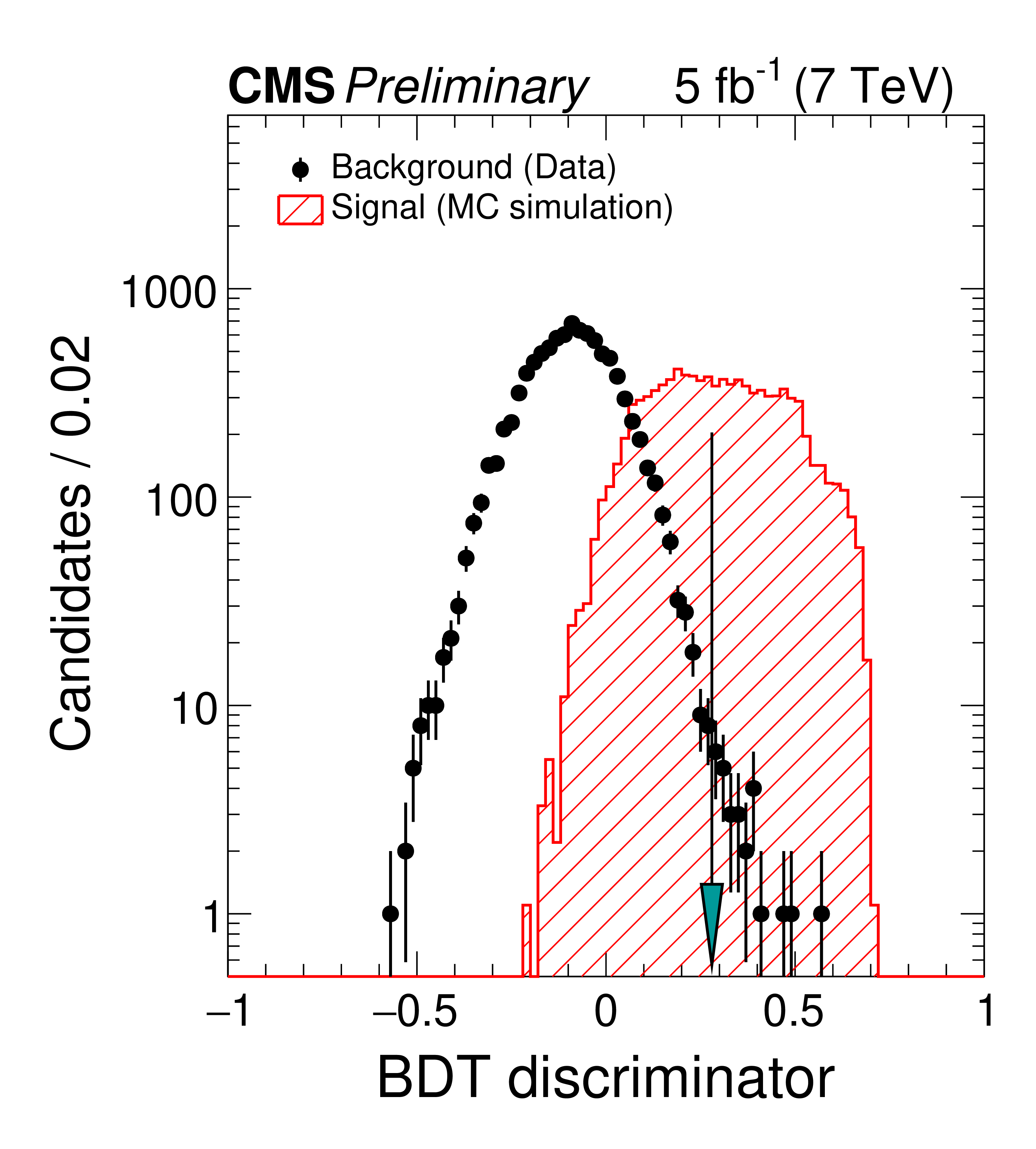
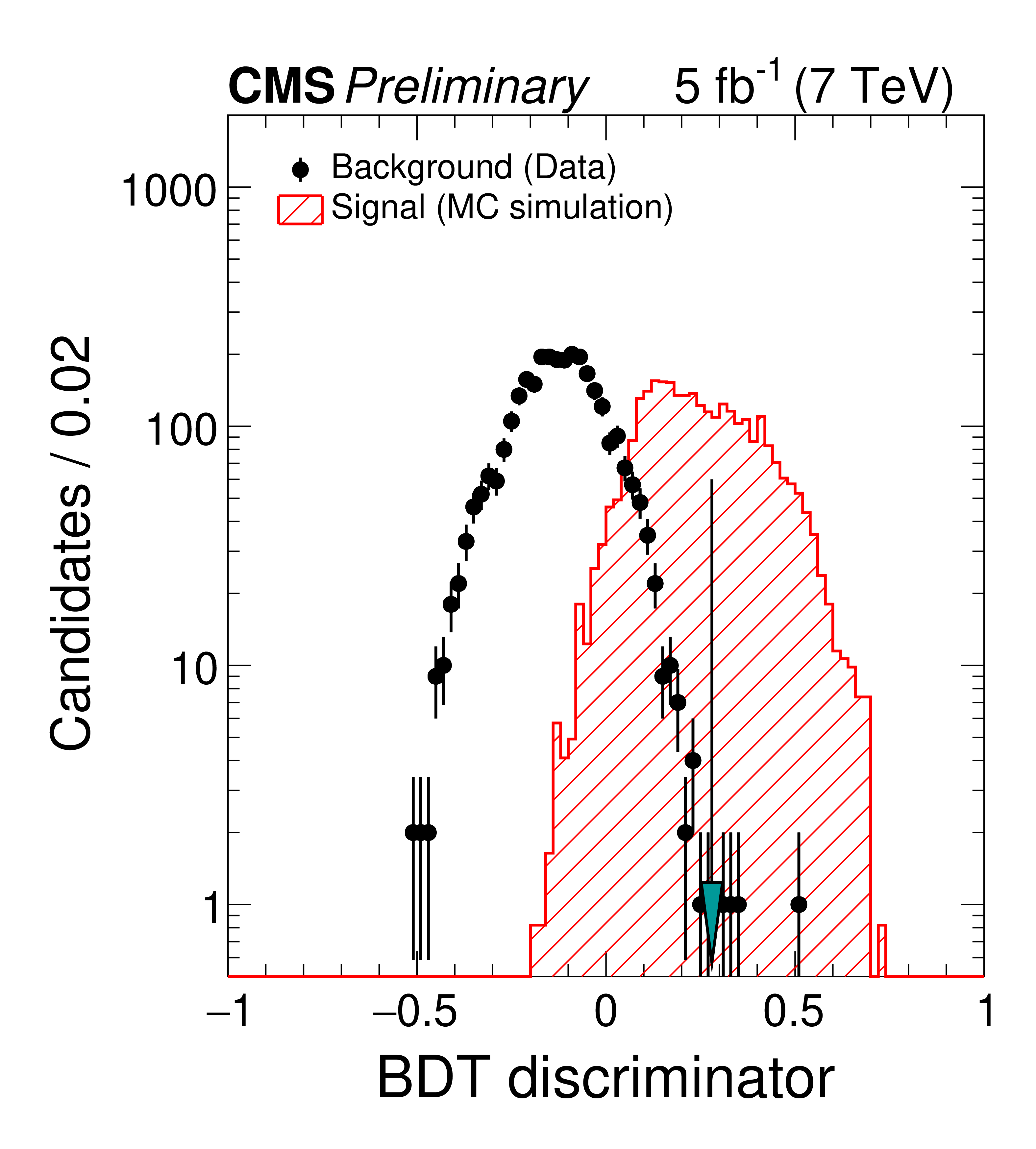
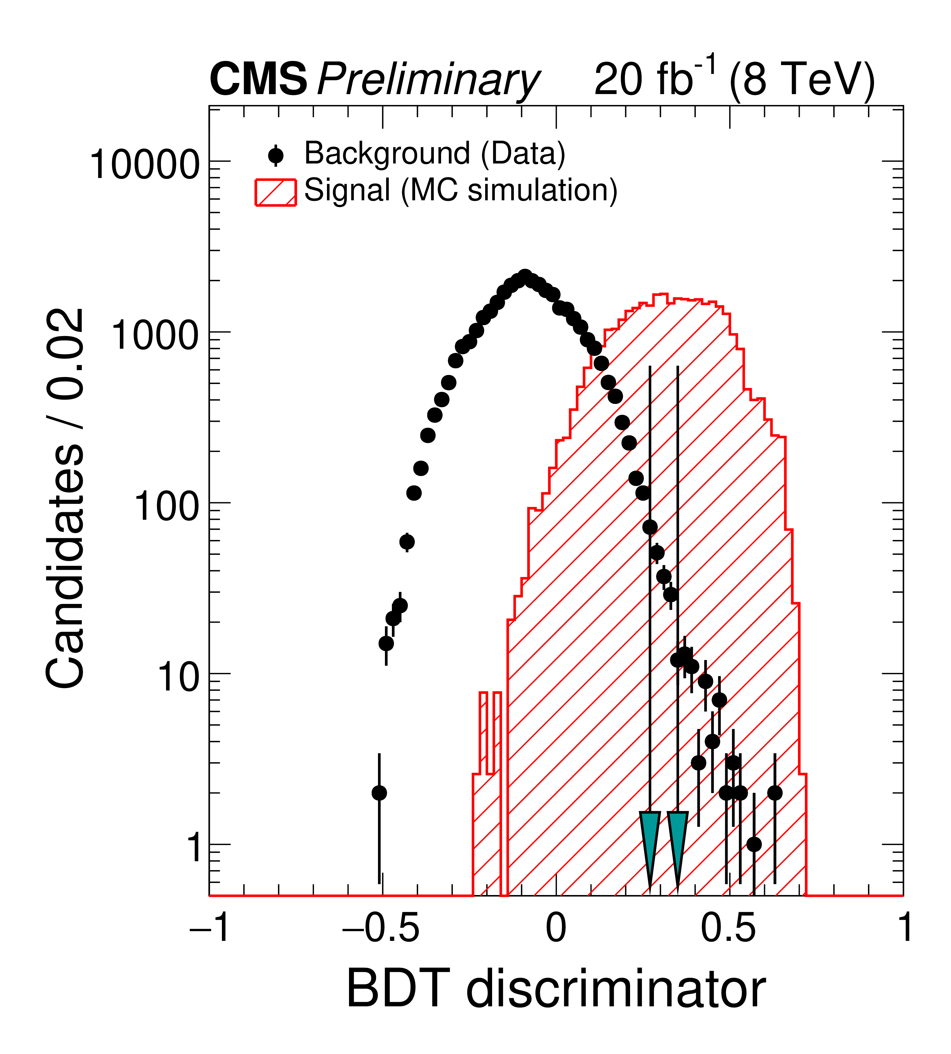
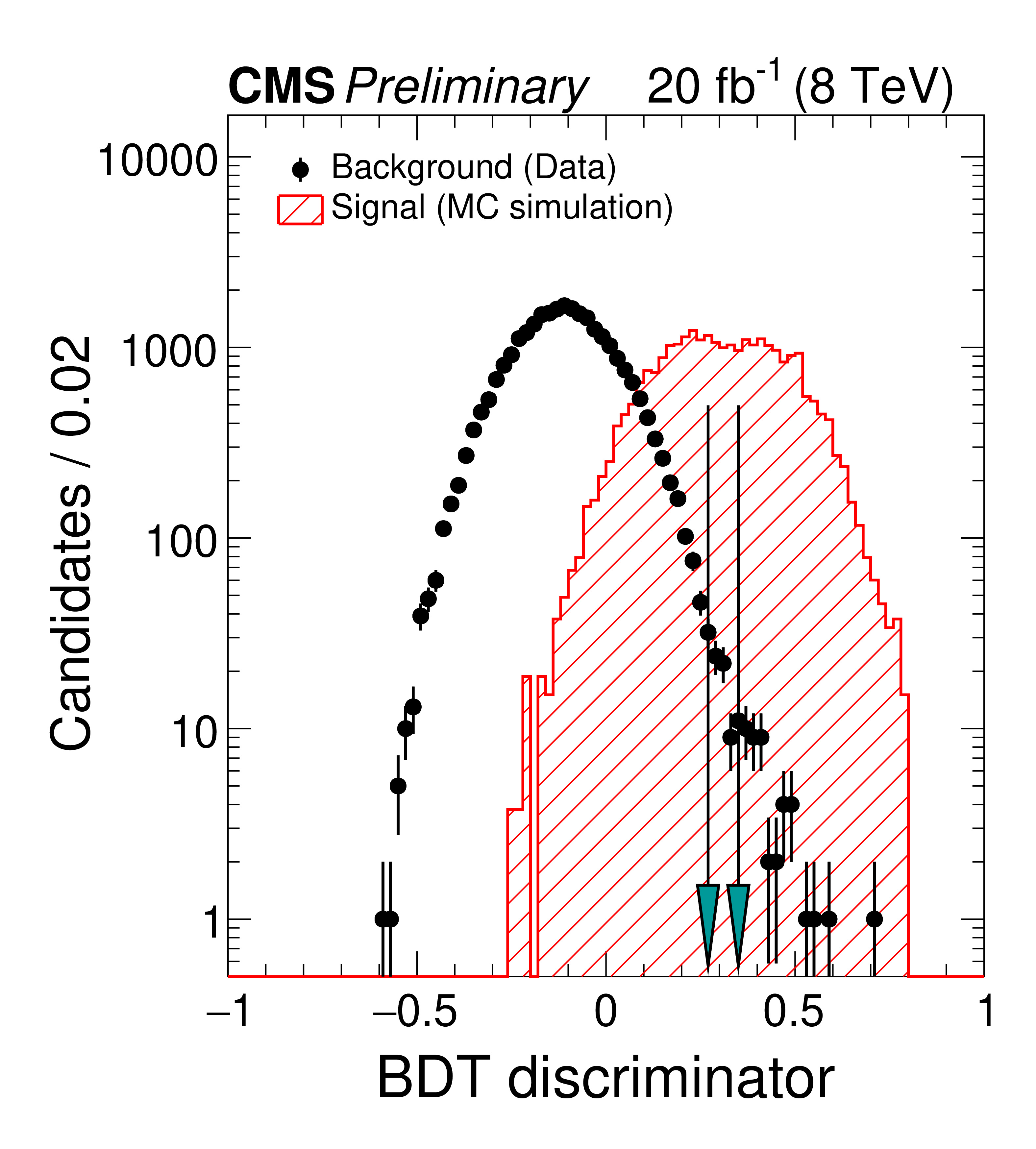
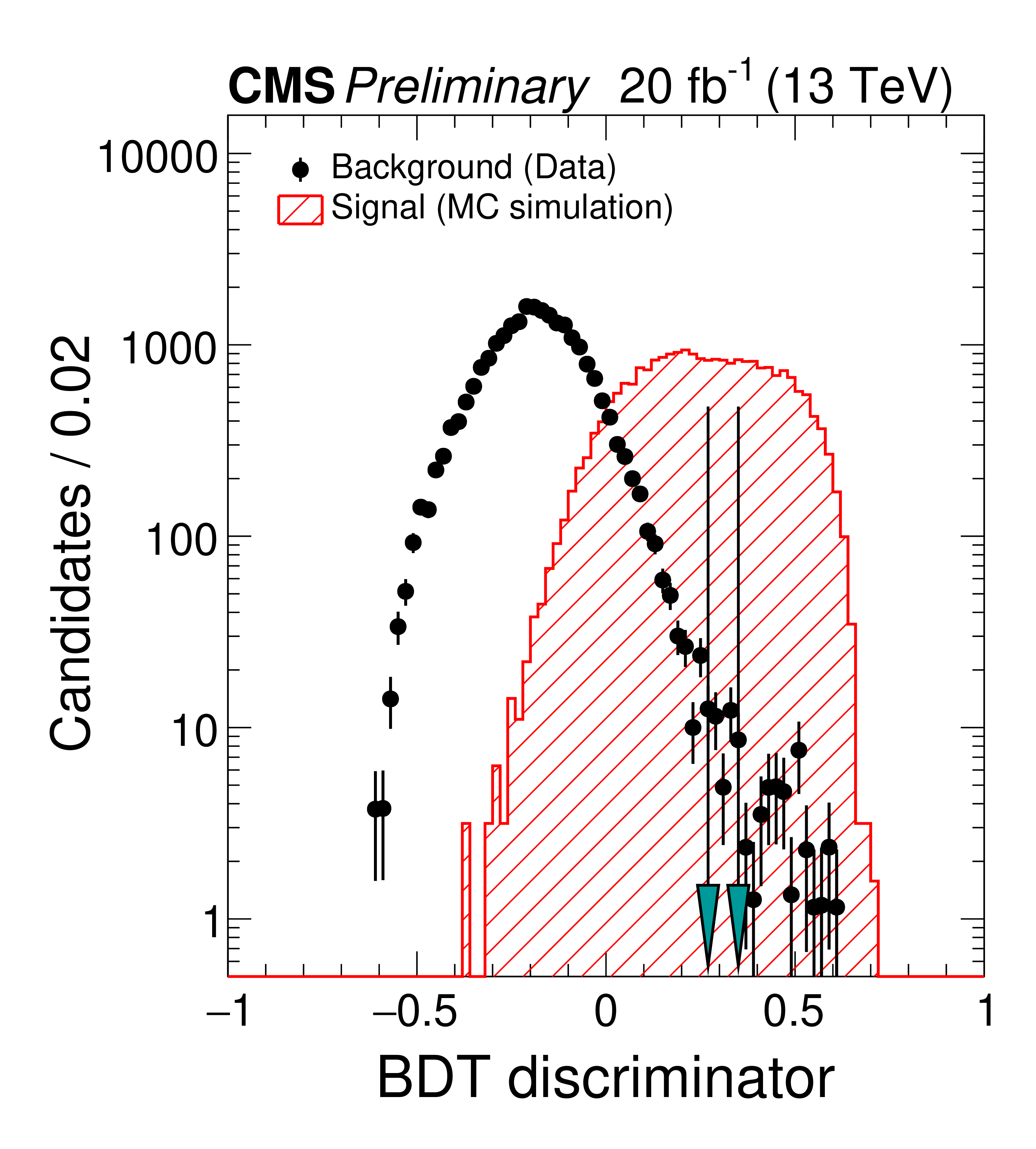
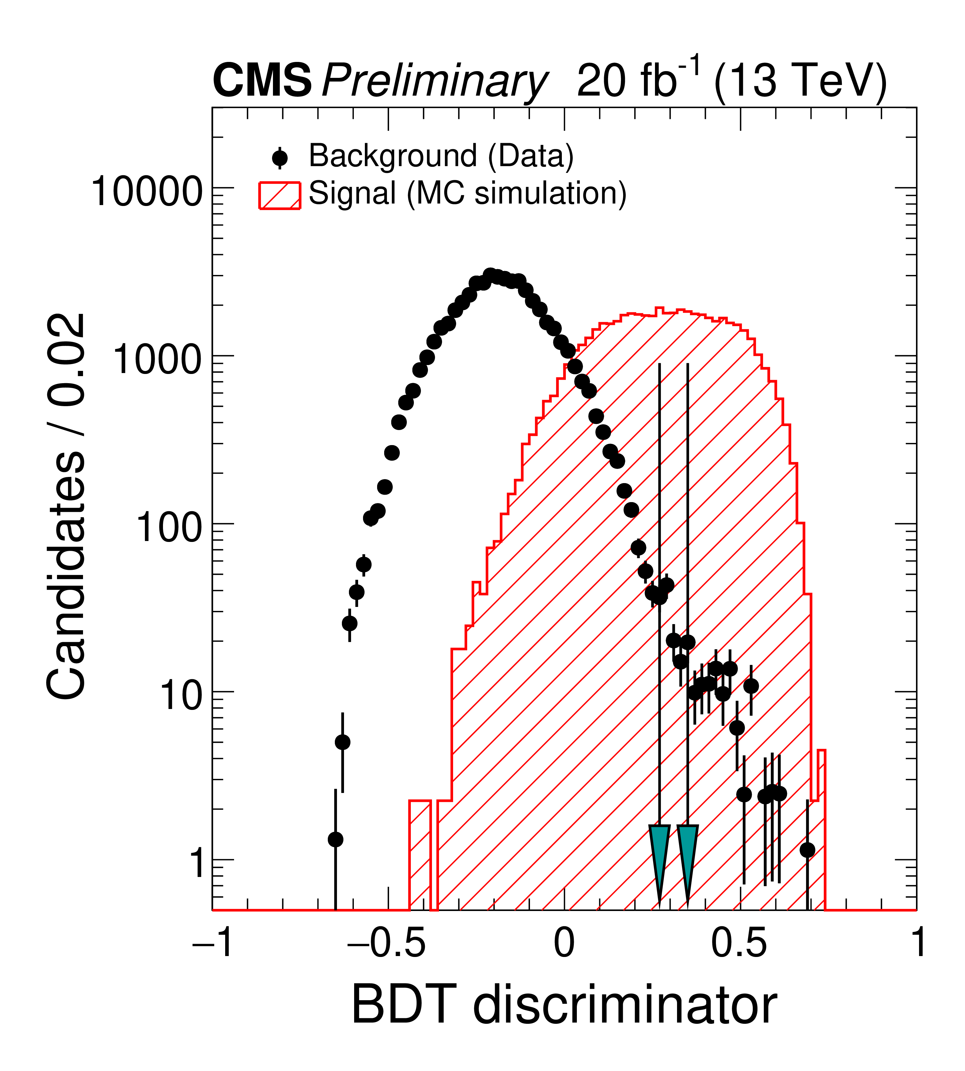
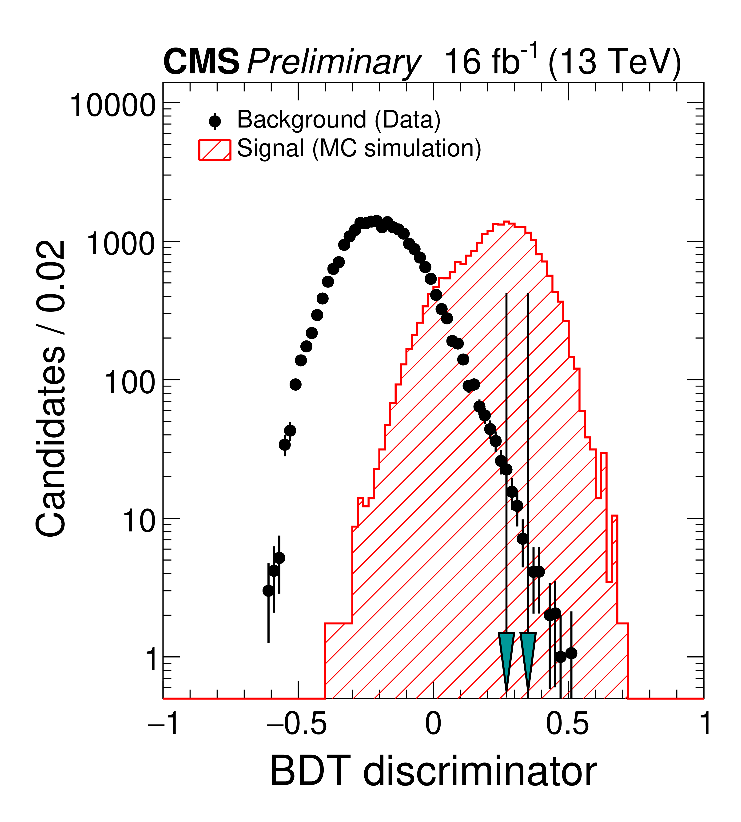
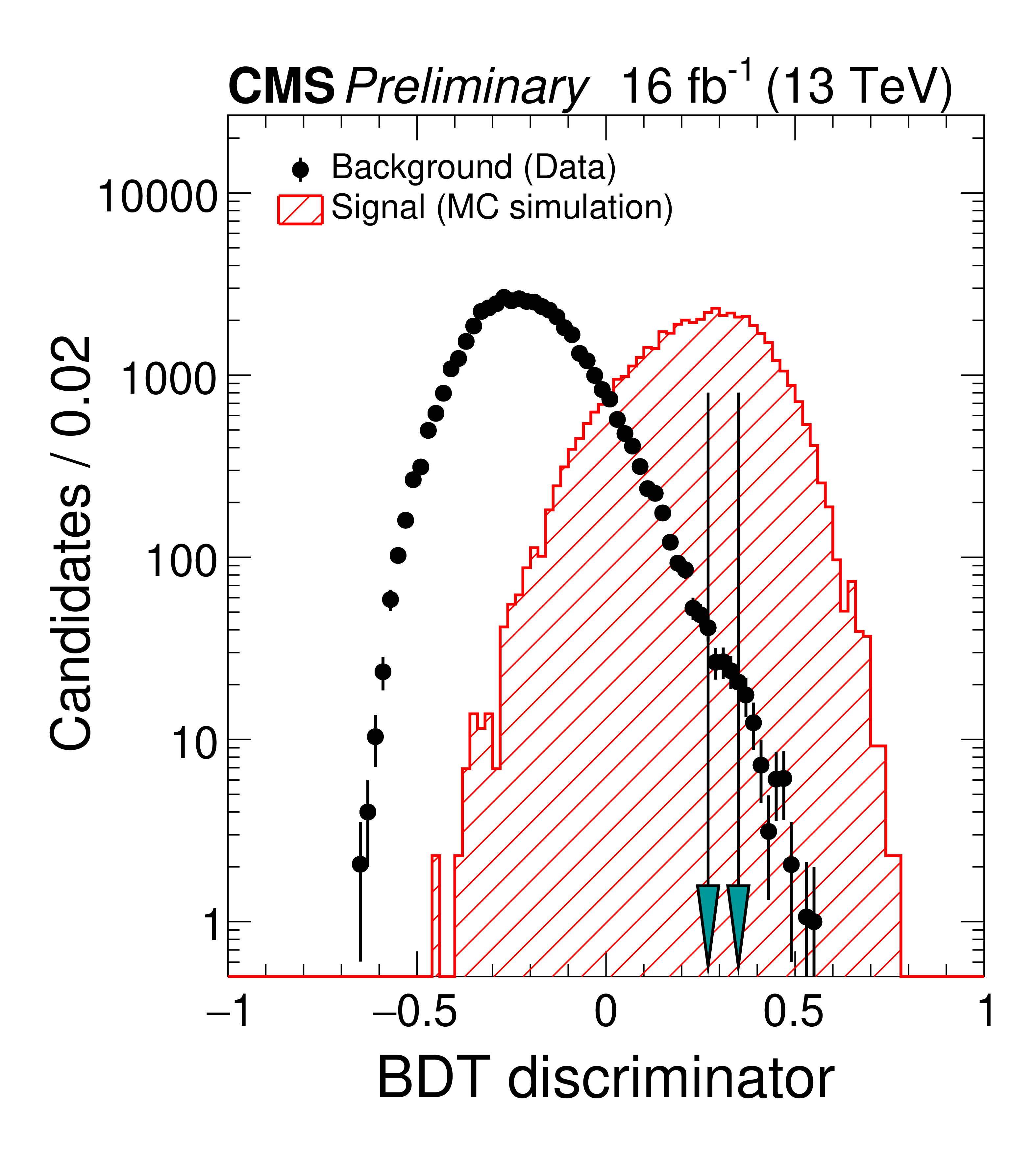
Figure 4:
(Top row) Illustration of the analysis BDT discriminator distributions in the central analysis channel for ${\mathrm{B^{+}} \to {\mathrm{J}/\psi} \mathrm{K^{+}}} $ in background-subtracted data and MC simulation in the central channel for 2011 (left column), 2012 (middle column), and 2016B (right column). (Bottom row) Illustration of the analysis BDT discriminator distribution in dimuon background data from the 5.45 $ < {m_{\mu^{+} \mu^{-}}} < $ 5.9 GeV sideband and ${\mathrm{B}^{0}s \to \mu^{+} \mu^{-}} $ signal MC simulation. The distributions correspond to the full preselection and are normalized to the same number of entries. The solid markers show the data and the hatched histogram the MC simulation. The arrows show the BDT discriminator boundaries provided in Table 1. The band in the ratio plot shows the $ \pm $20% variation. |
png pdf |
Figure 4-a:
(Top row) Illustration of the analysis BDT discriminator distributions in the central analysis channel for ${\mathrm{B^{+}} \to {\mathrm{J}/\psi} \mathrm{K^{+}}} $ in background-subtracted data and MC simulation in the central channel for 2011 (left column), 2012 (middle column), and 2016B (right column). (Bottom row) Illustration of the analysis BDT discriminator distribution in dimuon background data from the 5.45 $ < {m_{\mu^{+} \mu^{-}}} < $ 5.9 GeV sideband and ${\mathrm{B}^{0}s \to \mu^{+} \mu^{-}} $ signal MC simulation. The distributions correspond to the full preselection and are normalized to the same number of entries. The solid markers show the data and the hatched histogram the MC simulation. The arrows show the BDT discriminator boundaries provided in Table 1. The band in the ratio plot shows the $ \pm $20% variation. |
png pdf |
Figure 4-b:
(Top row) Illustration of the analysis BDT discriminator distributions in the central analysis channel for ${\mathrm{B^{+}} \to {\mathrm{J}/\psi} \mathrm{K^{+}}} $ in background-subtracted data and MC simulation in the central channel for 2011 (left column), 2012 (middle column), and 2016B (right column). (Bottom row) Illustration of the analysis BDT discriminator distribution in dimuon background data from the 5.45 $ < {m_{\mu^{+} \mu^{-}}} < $ 5.9 GeV sideband and ${\mathrm{B}^{0}s \to \mu^{+} \mu^{-}} $ signal MC simulation. The distributions correspond to the full preselection and are normalized to the same number of entries. The solid markers show the data and the hatched histogram the MC simulation. The arrows show the BDT discriminator boundaries provided in Table 1. The band in the ratio plot shows the $ \pm $20% variation. |
png pdf |
Figure 4-c:
(Top row) Illustration of the analysis BDT discriminator distributions in the central analysis channel for ${\mathrm{B^{+}} \to {\mathrm{J}/\psi} \mathrm{K^{+}}} $ in background-subtracted data and MC simulation in the central channel for 2011 (left column), 2012 (middle column), and 2016B (right column). (Bottom row) Illustration of the analysis BDT discriminator distribution in dimuon background data from the 5.45 $ < {m_{\mu^{+} \mu^{-}}} < $ 5.9 GeV sideband and ${\mathrm{B}^{0}s \to \mu^{+} \mu^{-}} $ signal MC simulation. The distributions correspond to the full preselection and are normalized to the same number of entries. The solid markers show the data and the hatched histogram the MC simulation. The arrows show the BDT discriminator boundaries provided in Table 1. The band in the ratio plot shows the $ \pm $20% variation. |
png pdf |
Figure 4-d:
(Top row) Illustration of the analysis BDT discriminator distributions in the central analysis channel for ${\mathrm{B^{+}} \to {\mathrm{J}/\psi} \mathrm{K^{+}}} $ in background-subtracted data and MC simulation in the central channel for 2011 (left column), 2012 (middle column), and 2016B (right column). (Bottom row) Illustration of the analysis BDT discriminator distribution in dimuon background data from the 5.45 $ < {m_{\mu^{+} \mu^{-}}} < $ 5.9 GeV sideband and ${\mathrm{B}^{0}s \to \mu^{+} \mu^{-}} $ signal MC simulation. The distributions correspond to the full preselection and are normalized to the same number of entries. The solid markers show the data and the hatched histogram the MC simulation. The arrows show the BDT discriminator boundaries provided in Table 1. The band in the ratio plot shows the $ \pm $20% variation. |
png pdf |
Figure 4-e:
(Top row) Illustration of the analysis BDT discriminator distributions in the central analysis channel for ${\mathrm{B^{+}} \to {\mathrm{J}/\psi} \mathrm{K^{+}}} $ in background-subtracted data and MC simulation in the central channel for 2011 (left column), 2012 (middle column), and 2016B (right column). (Bottom row) Illustration of the analysis BDT discriminator distribution in dimuon background data from the 5.45 $ < {m_{\mu^{+} \mu^{-}}} < $ 5.9 GeV sideband and ${\mathrm{B}^{0}s \to \mu^{+} \mu^{-}} $ signal MC simulation. The distributions correspond to the full preselection and are normalized to the same number of entries. The solid markers show the data and the hatched histogram the MC simulation. The arrows show the BDT discriminator boundaries provided in Table 1. The band in the ratio plot shows the $ \pm $20% variation. |
png pdf |
Figure 4-f:
(Top row) Illustration of the analysis BDT discriminator distributions in the central analysis channel for ${\mathrm{B^{+}} \to {\mathrm{J}/\psi} \mathrm{K^{+}}} $ in background-subtracted data and MC simulation in the central channel for 2011 (left column), 2012 (middle column), and 2016B (right column). (Bottom row) Illustration of the analysis BDT discriminator distribution in dimuon background data from the 5.45 $ < {m_{\mu^{+} \mu^{-}}} < $ 5.9 GeV sideband and ${\mathrm{B}^{0}s \to \mu^{+} \mu^{-}} $ signal MC simulation. The distributions correspond to the full preselection and are normalized to the same number of entries. The solid markers show the data and the hatched histogram the MC simulation. The arrows show the BDT discriminator boundaries provided in Table 1. The band in the ratio plot shows the $ \pm $20% variation. |
png pdf |
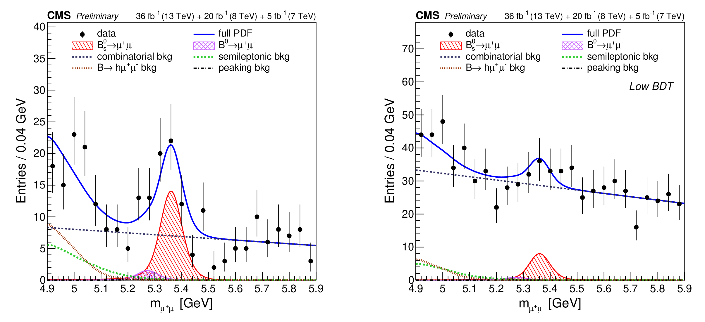
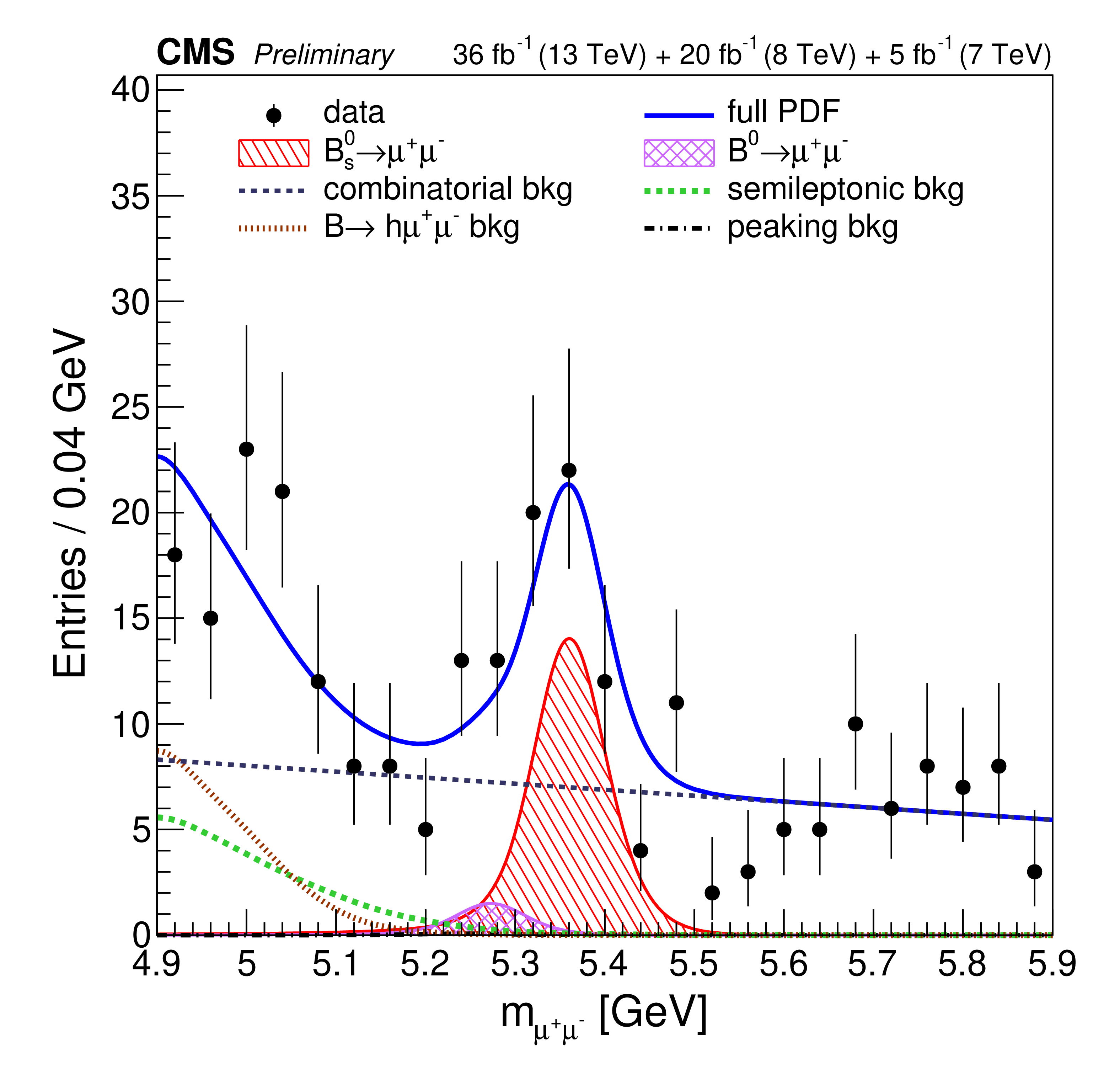
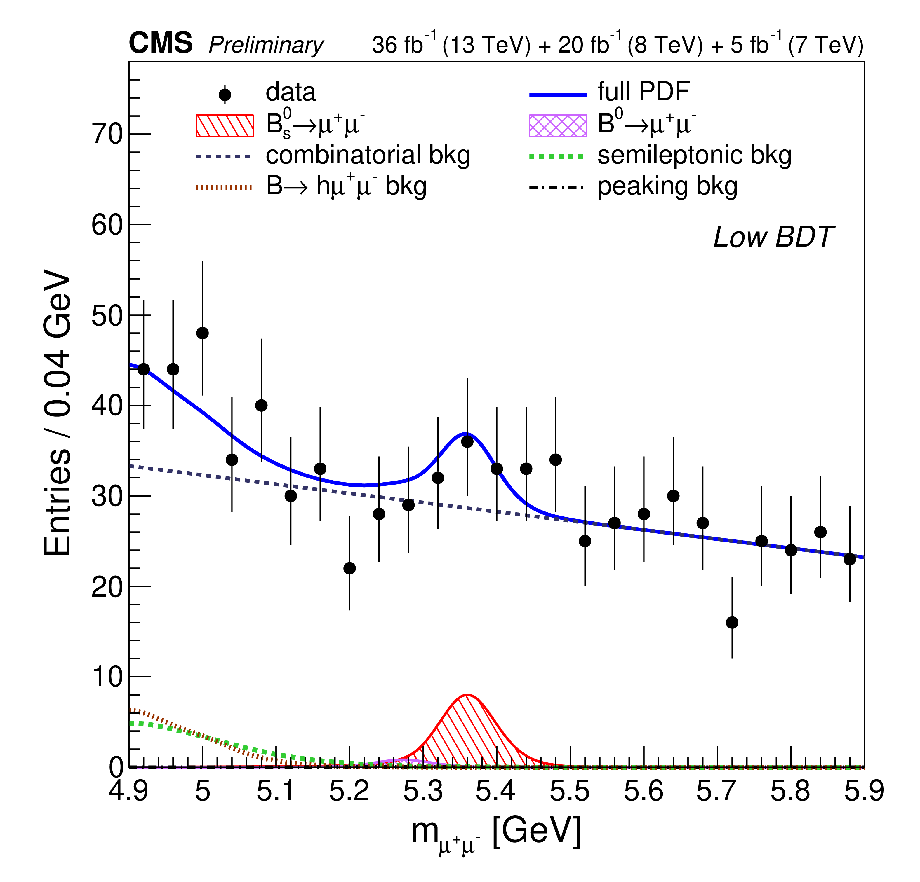
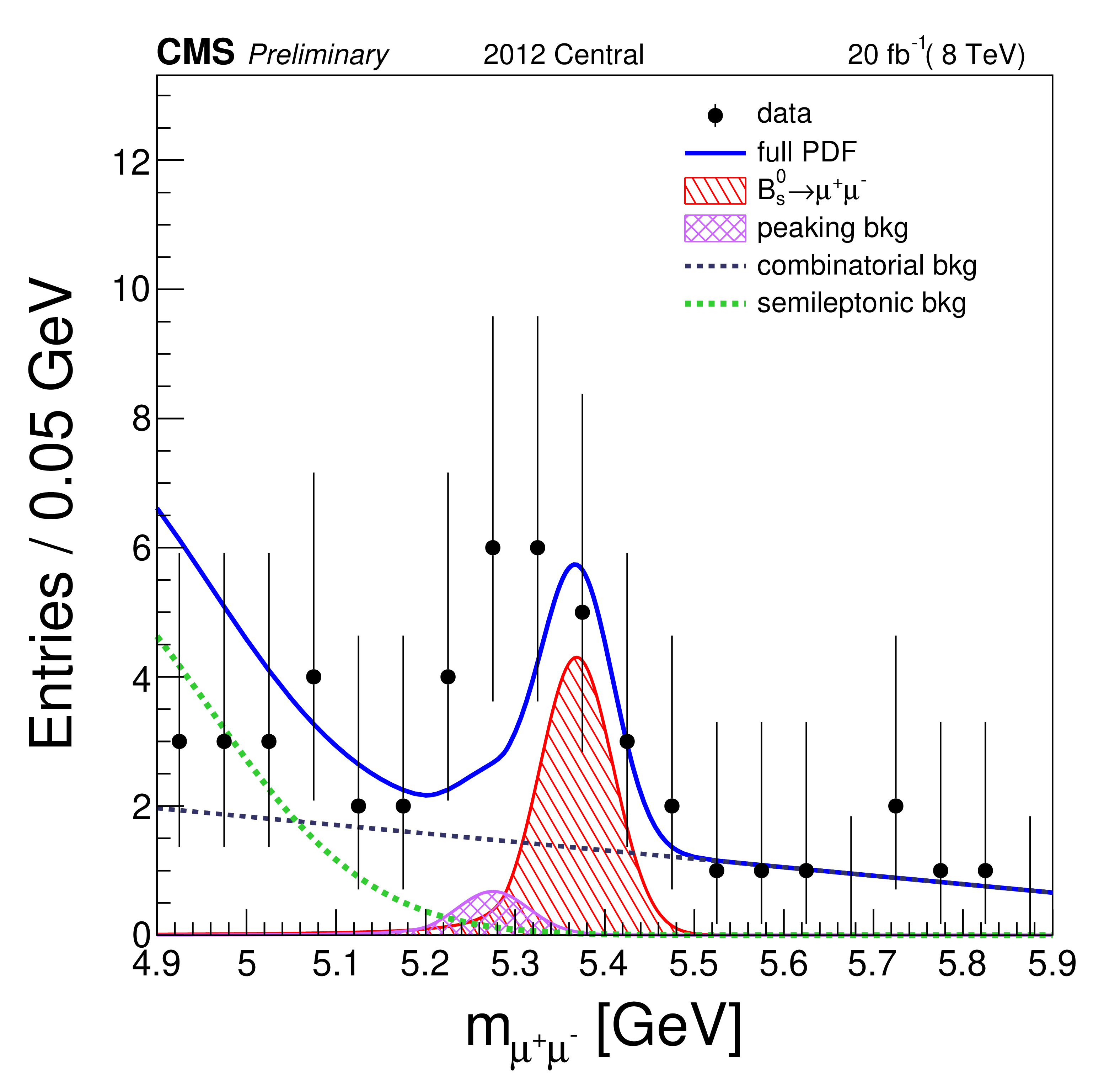
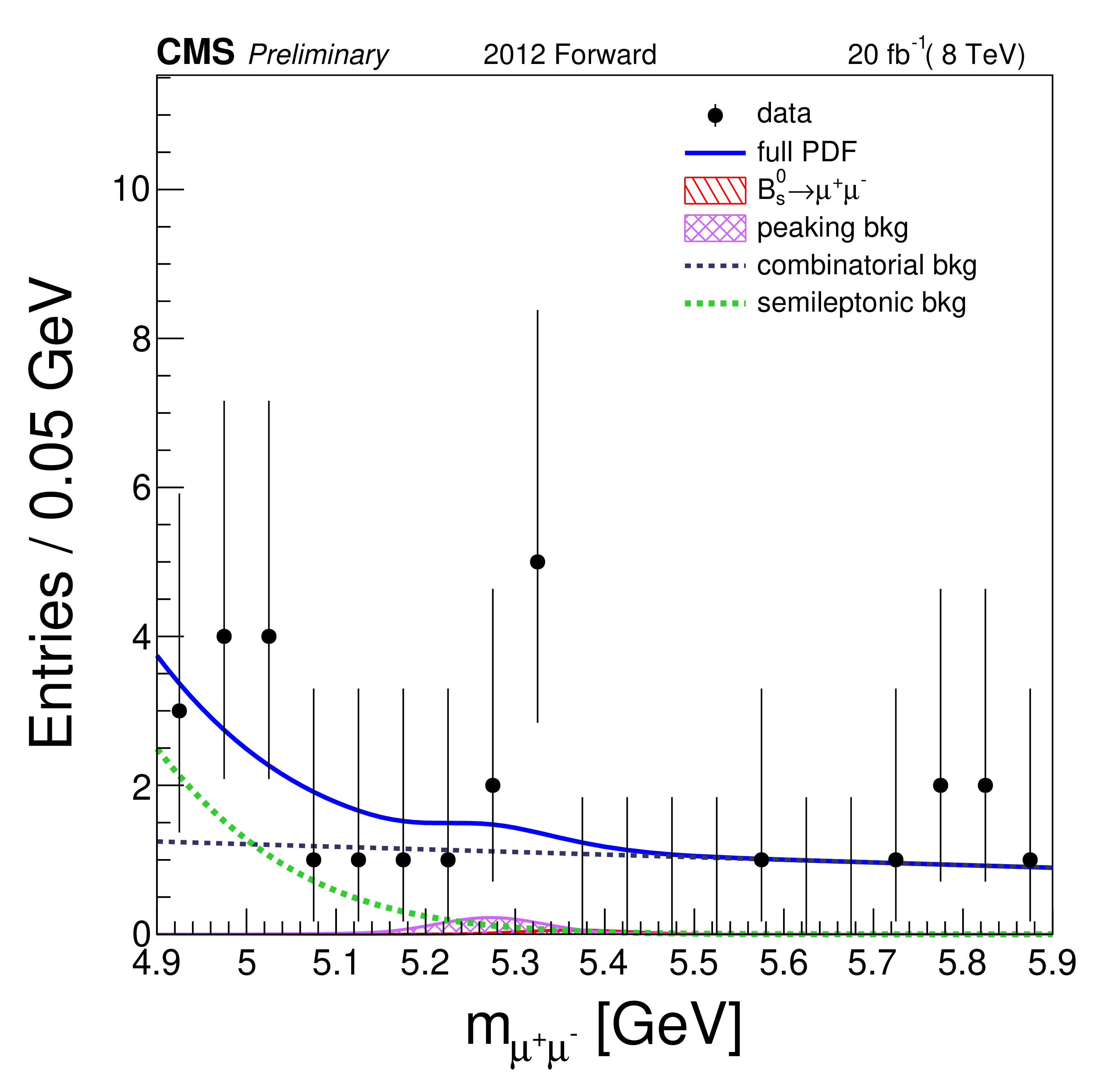
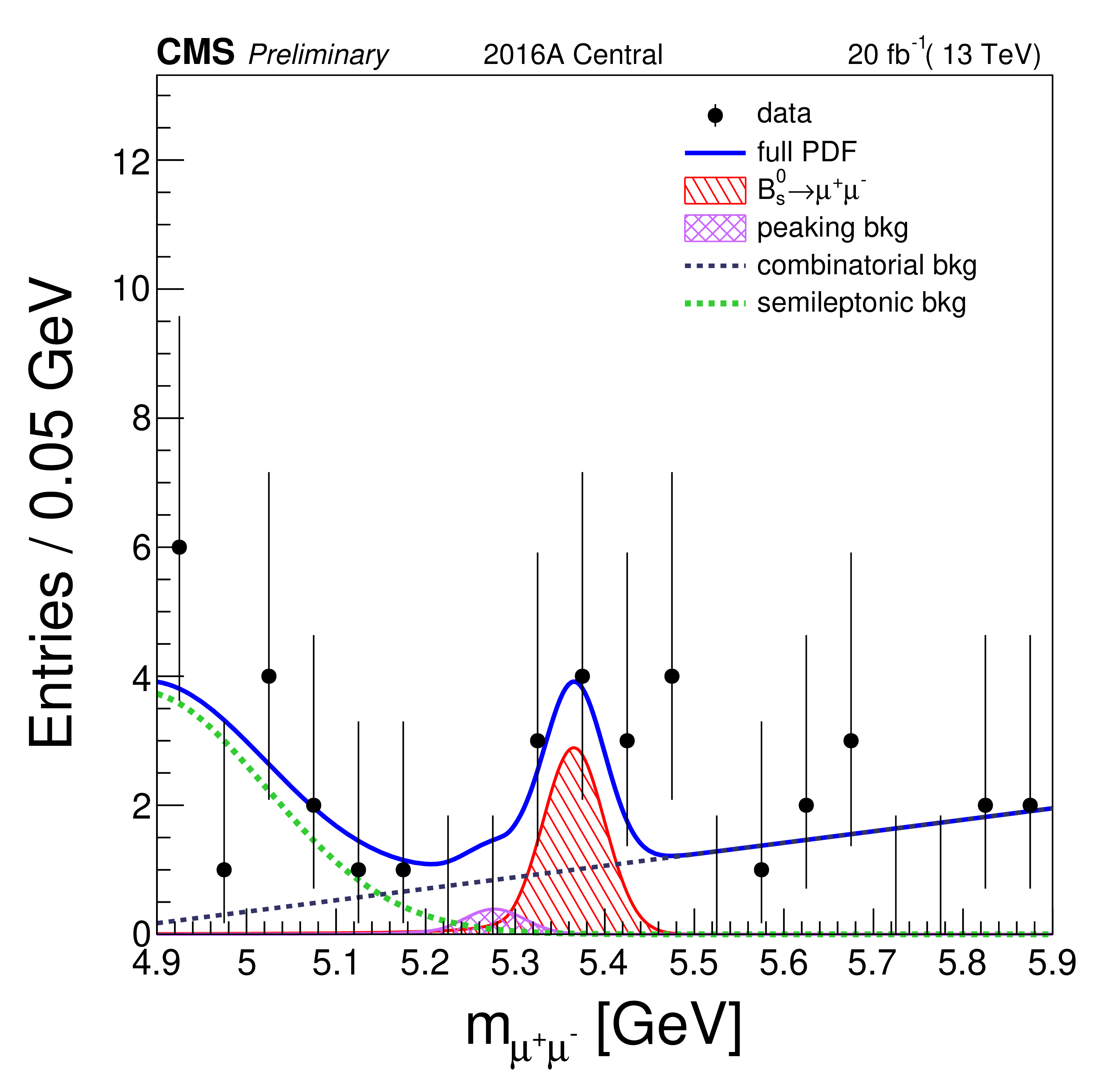
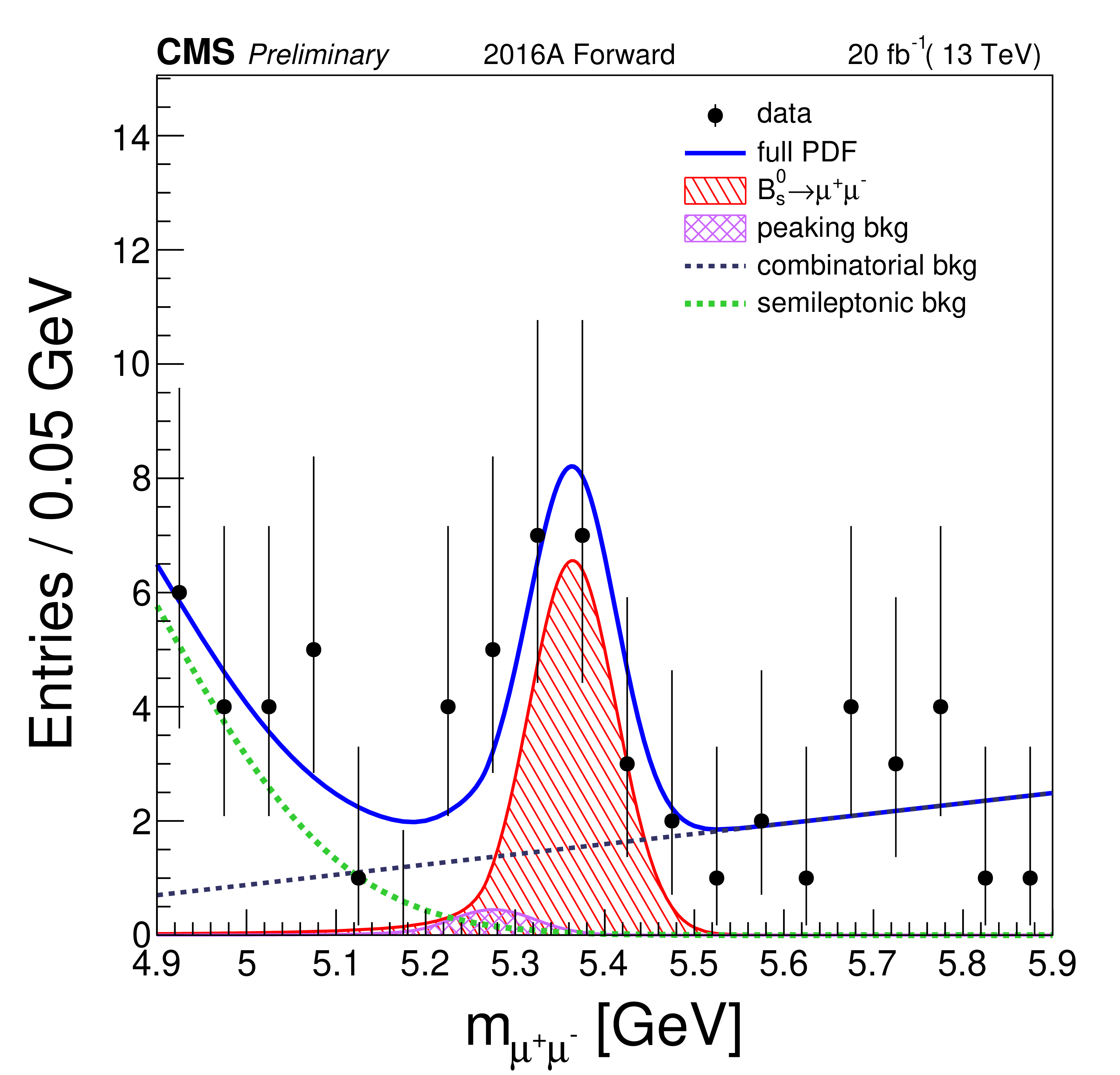
Figure 5:
Invariant mass distributions with the fit projection overlays for the branching fraction results. The left (right) plot shows the combined results from the high- (low-)range analysis BDT categories defined in Table 1. The total fit is shown by the solid line and the different background components by the broken lines. The signal components are shown by the hatched histograms. |
png pdf |
Figure 5-a:
Invariant mass distributions with the fit projection overlays for the branching fraction results. The left (right) plot shows the combined results from the high- (low-)range analysis BDT categories defined in Table 1. The total fit is shown by the solid line and the different background components by the broken lines. The signal components are shown by the hatched histograms. |
png pdf |
Figure 5-b:
Invariant mass distributions with the fit projection overlays for the branching fraction results. The left (right) plot shows the combined results from the high- (low-)range analysis BDT categories defined in Table 1. The total fit is shown by the solid line and the different background components by the broken lines. The signal components are shown by the hatched histograms. |
png pdf |
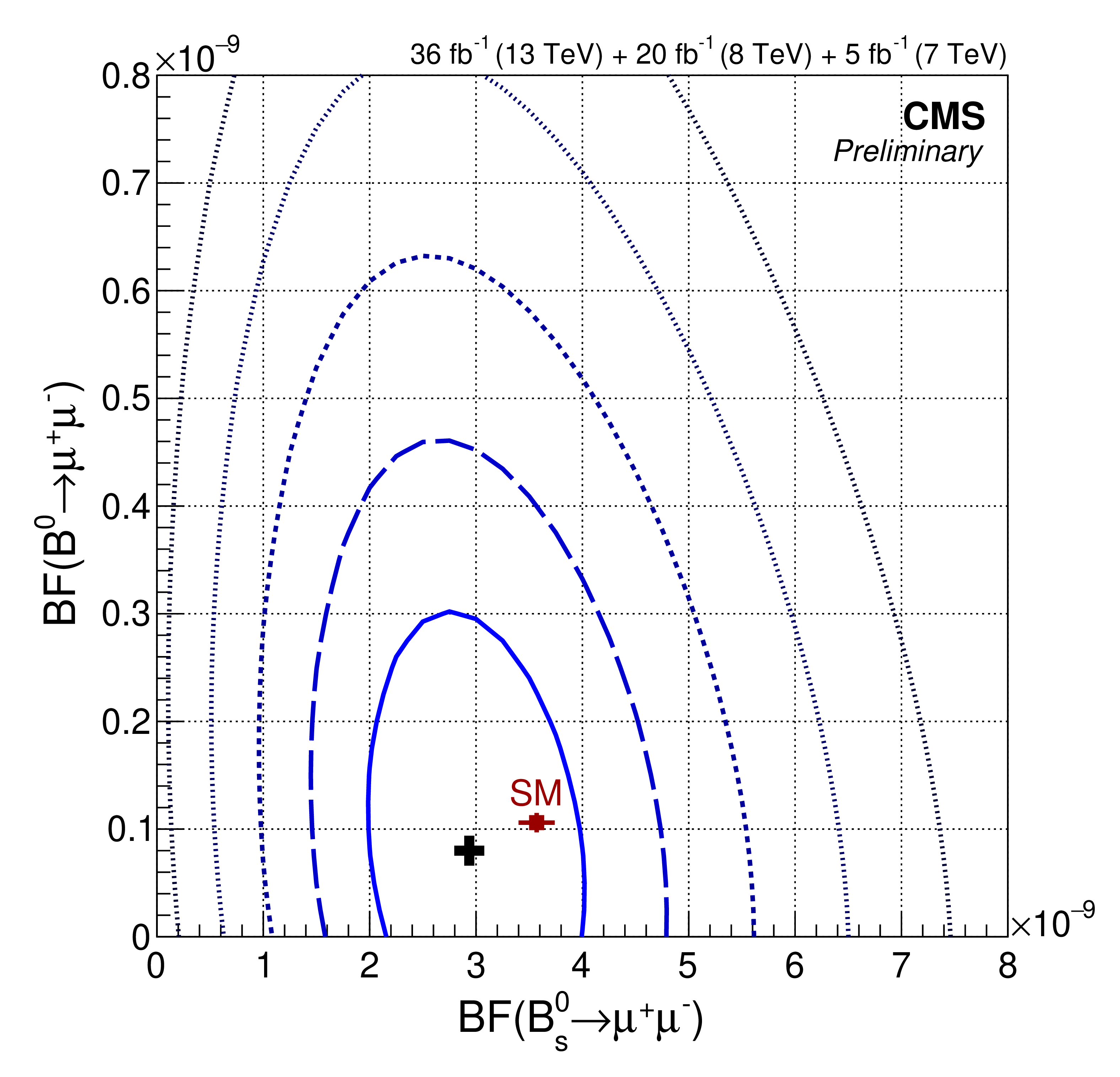
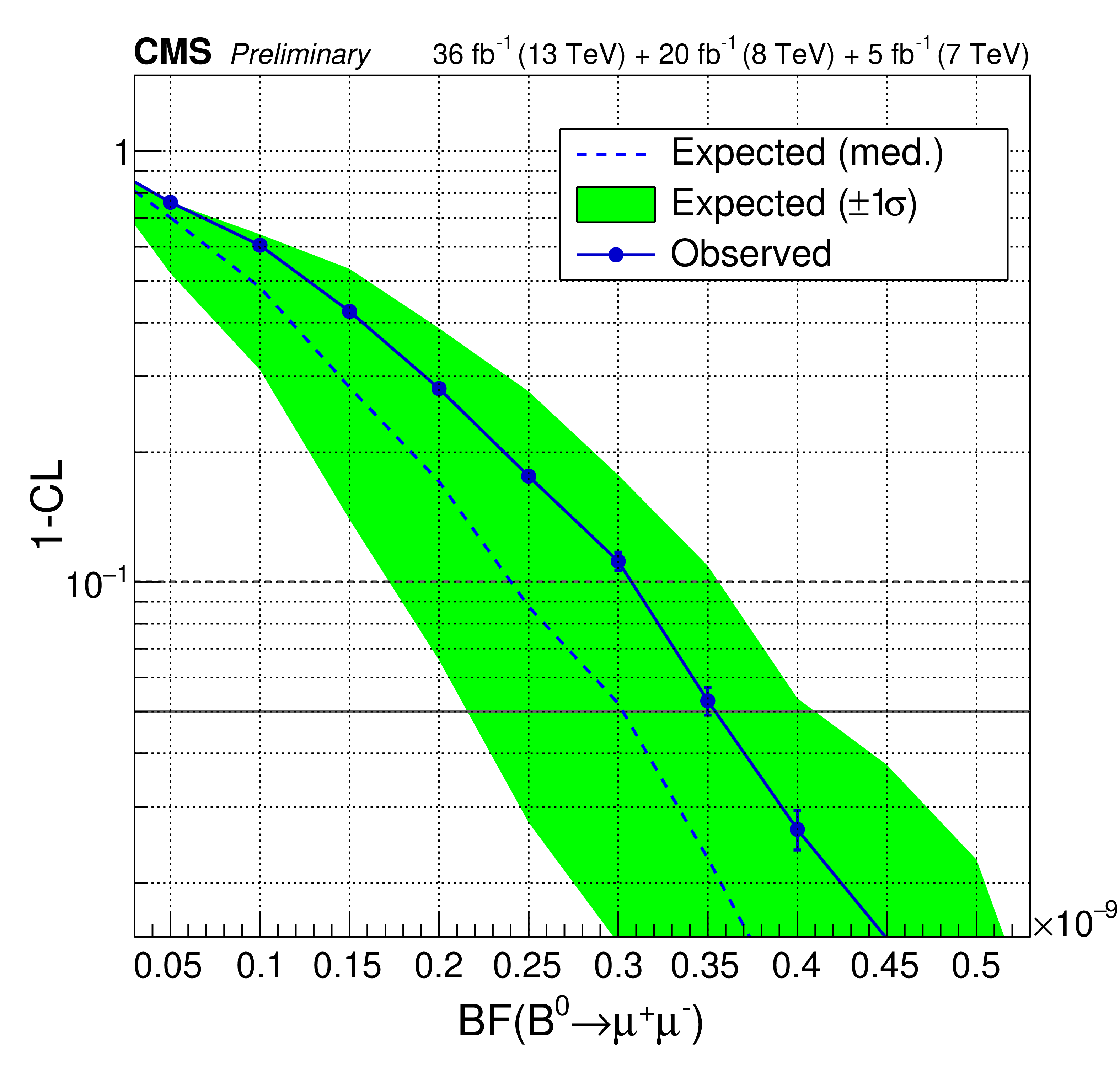
Figure 6:
(Left) Likelihood contours for the fit to the branching fractions $ {{\cal B}}({\mathrm{B}^{0}s \to \mu^{+} \mu^{-}})$ and $ {{\cal B}}({\mathrm{B}^{0} \to \mu^{+} \mu^{-}})$, together with the SM expectation. The contours correspond to regions with 1-5 standard deviation coverage. (Right) The quantity $1- CL $ as a function of the assumed ${\mathrm{B}^{0} \to \mu^{+} \mu^{-}}$ branching fraction. The dashed curve shows the median expected value for the background-only hypothesis while the solid line is the observed value. The green region indicates the 1 standard deviation uncertainty band. |
png pdf |
Figure 6-a:
(Left) Likelihood contours for the fit to the branching fractions $ {{\cal B}}({\mathrm{B}^{0}s \to \mu^{+} \mu^{-}})$ and $ {{\cal B}}({\mathrm{B}^{0} \to \mu^{+} \mu^{-}})$, together with the SM expectation. The contours correspond to regions with 1-5 standard deviation coverage. (Right) The quantity $1- CL $ as a function of the assumed ${\mathrm{B}^{0} \to \mu^{+} \mu^{-}}$ branching fraction. The dashed curve shows the median expected value for the background-only hypothesis while the solid line is the observed value. The green region indicates the 1 standard deviation uncertainty band. |
png pdf |
Figure 6-b:
(Left) Likelihood contours for the fit to the branching fractions $ {{\cal B}}({\mathrm{B}^{0}s \to \mu^{+} \mu^{-}})$ and $ {{\cal B}}({\mathrm{B}^{0} \to \mu^{+} \mu^{-}})$, together with the SM expectation. The contours correspond to regions with 1-5 standard deviation coverage. (Right) The quantity $1- CL $ as a function of the assumed ${\mathrm{B}^{0} \to \mu^{+} \mu^{-}}$ branching fraction. The dashed curve shows the median expected value for the background-only hypothesis while the solid line is the observed value. The green region indicates the 1 standard deviation uncertainty band. |
png pdf |
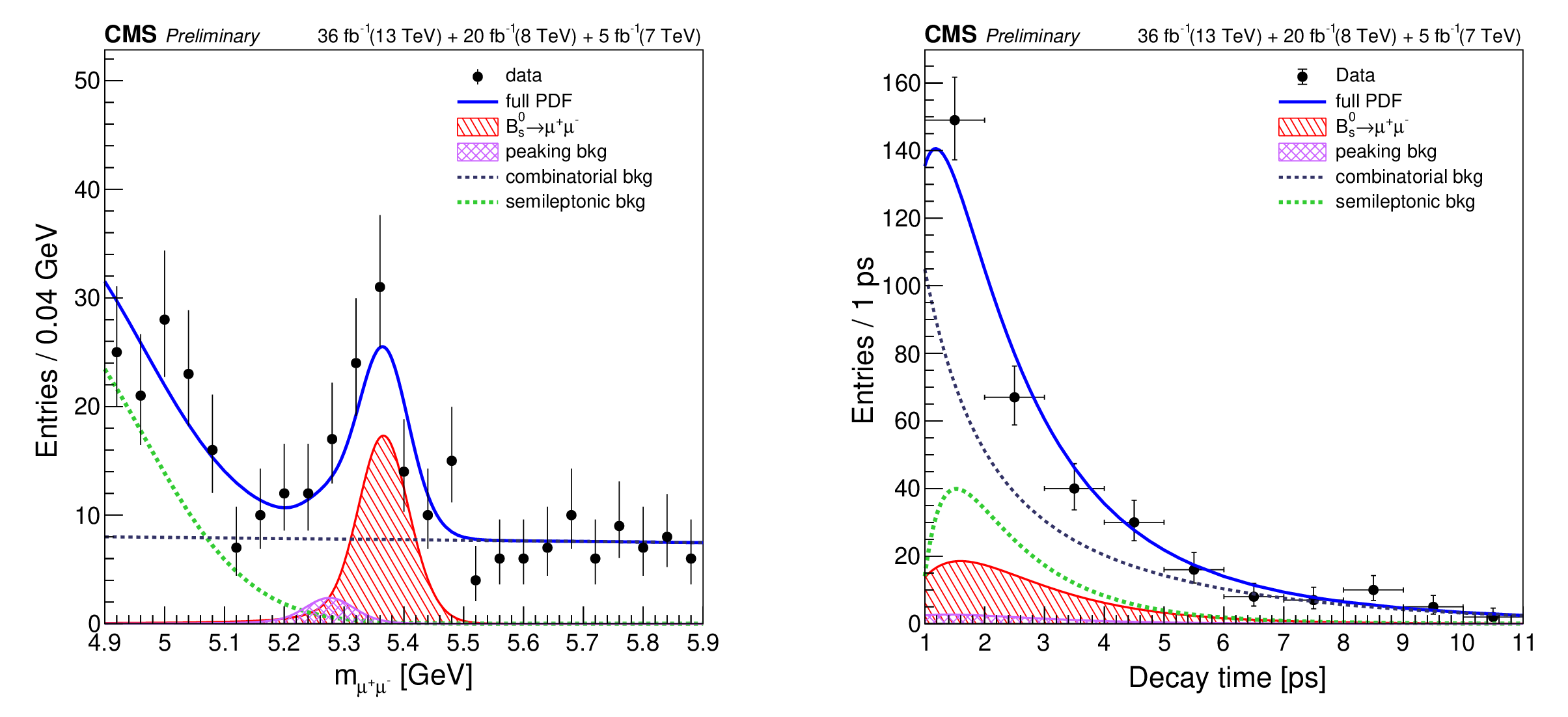
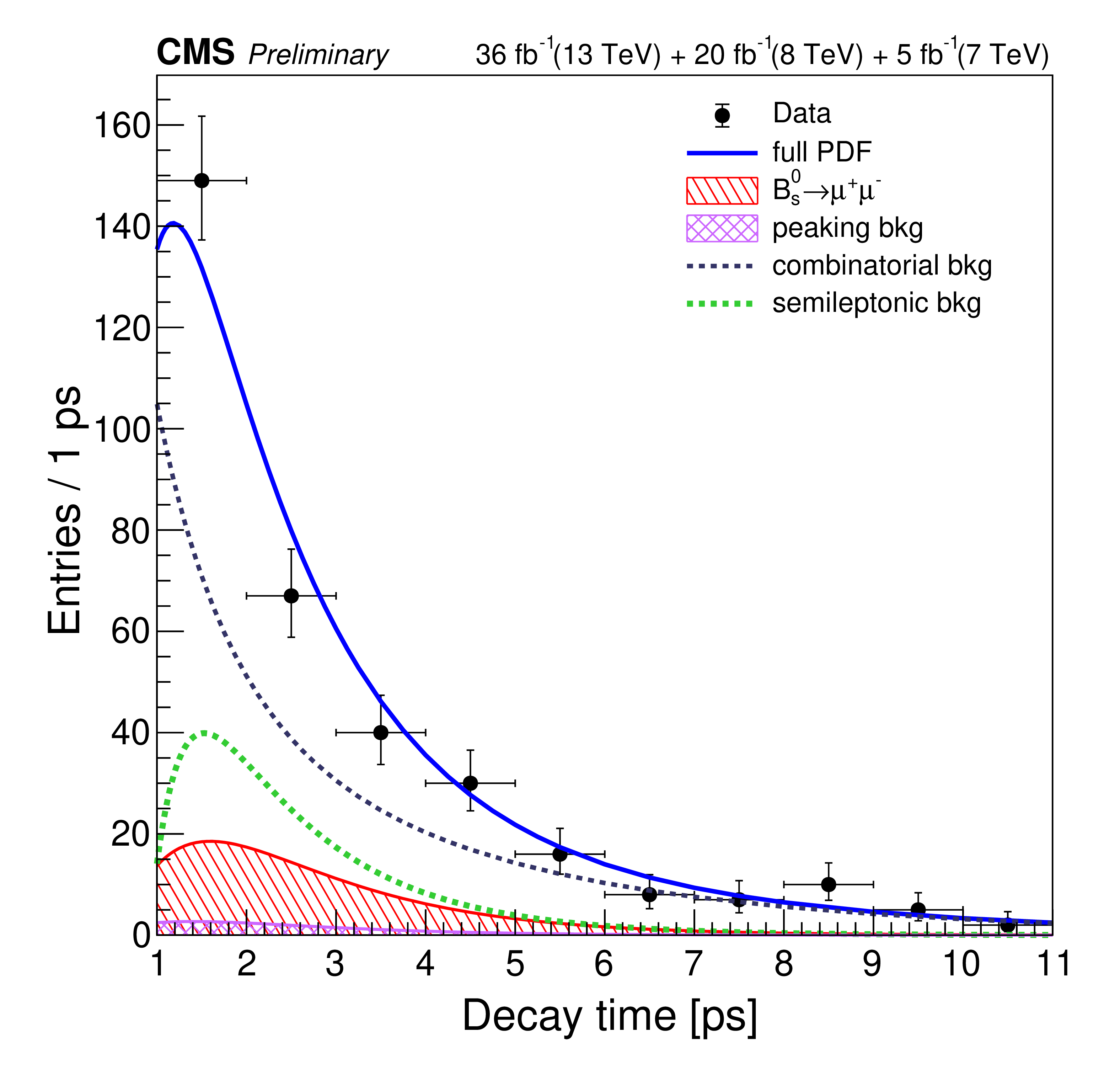
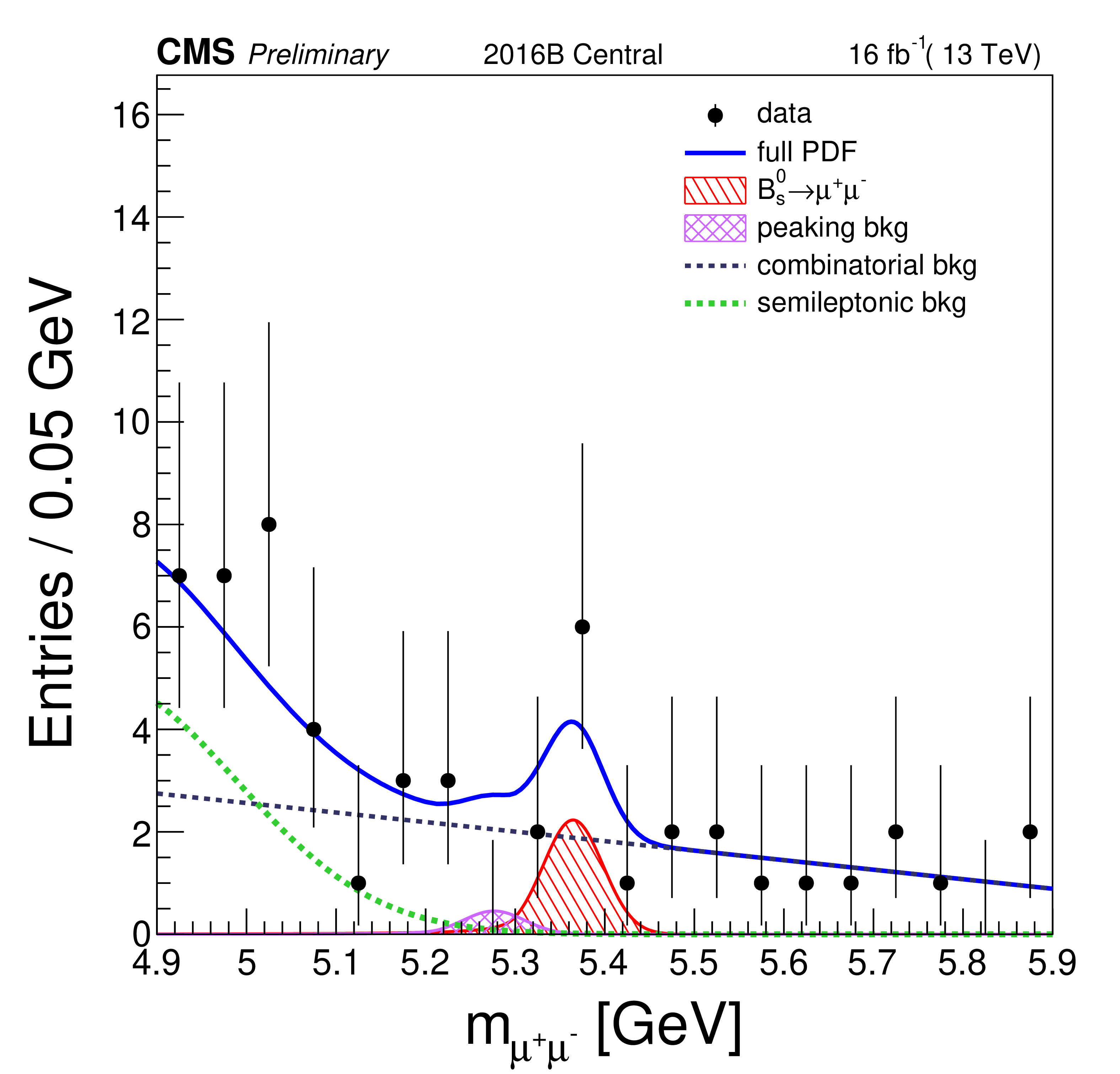
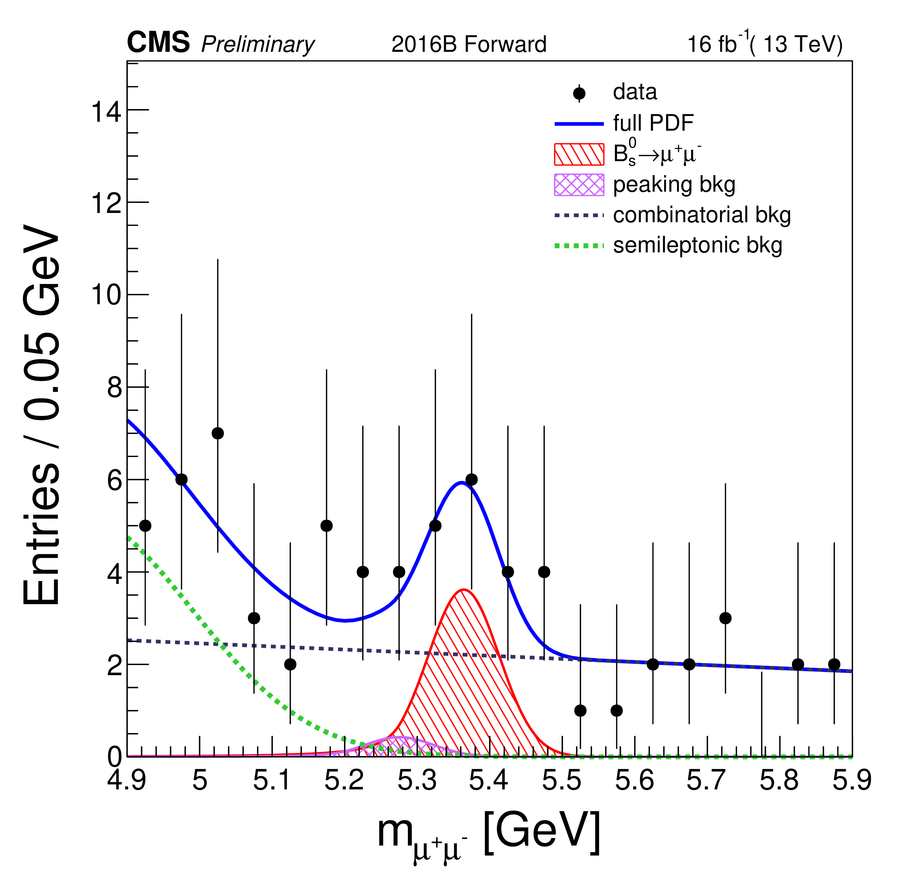
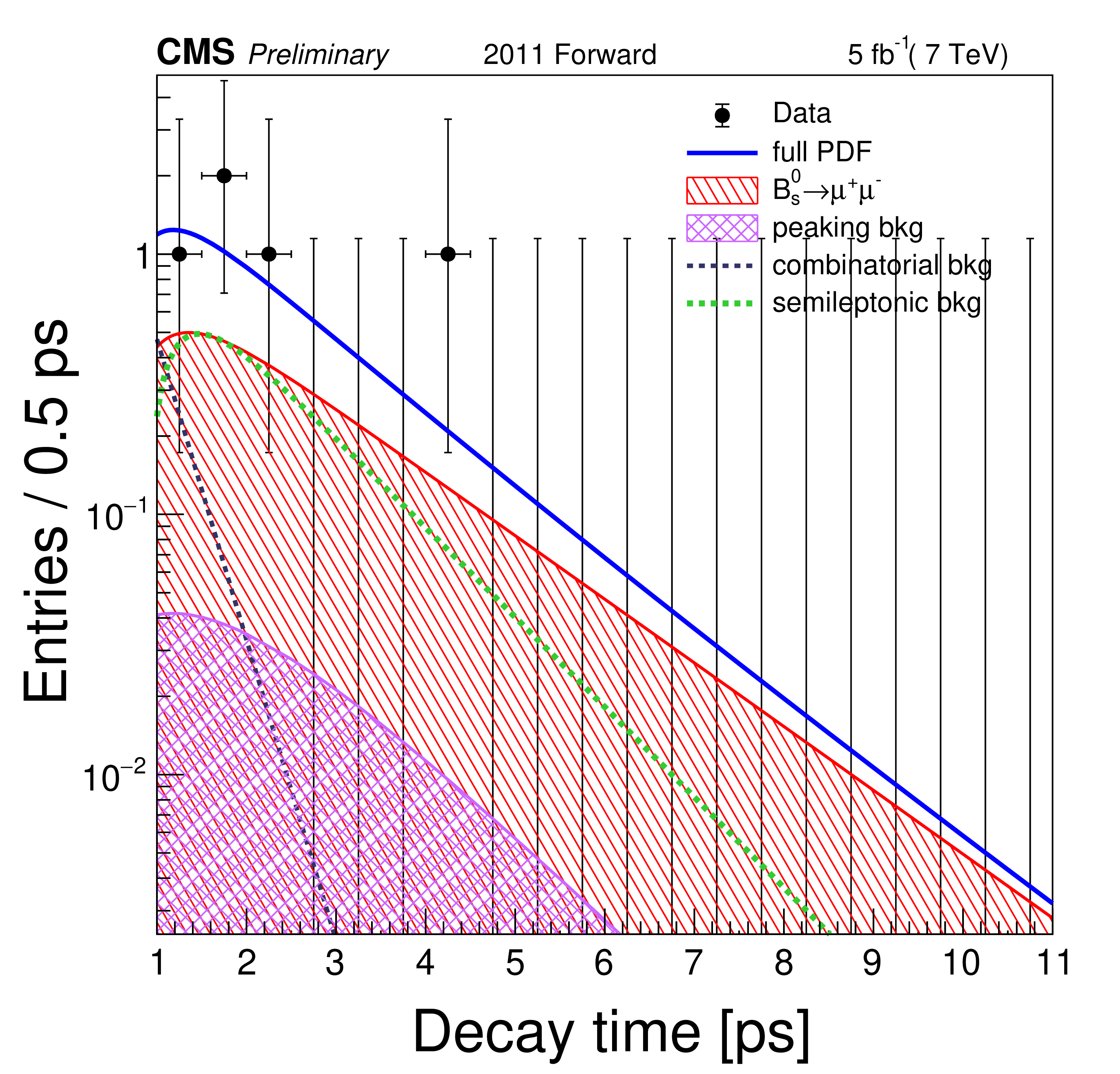
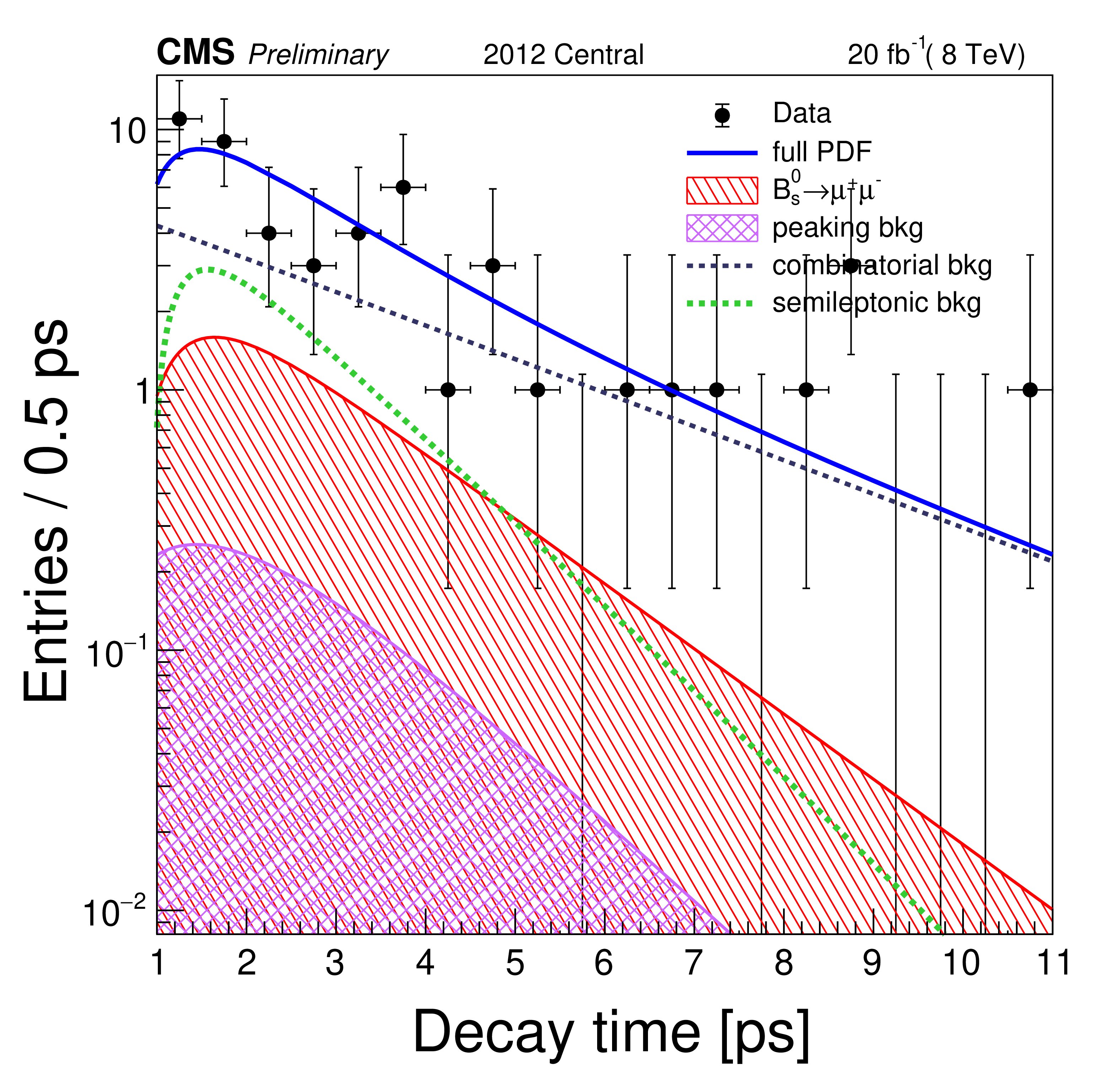
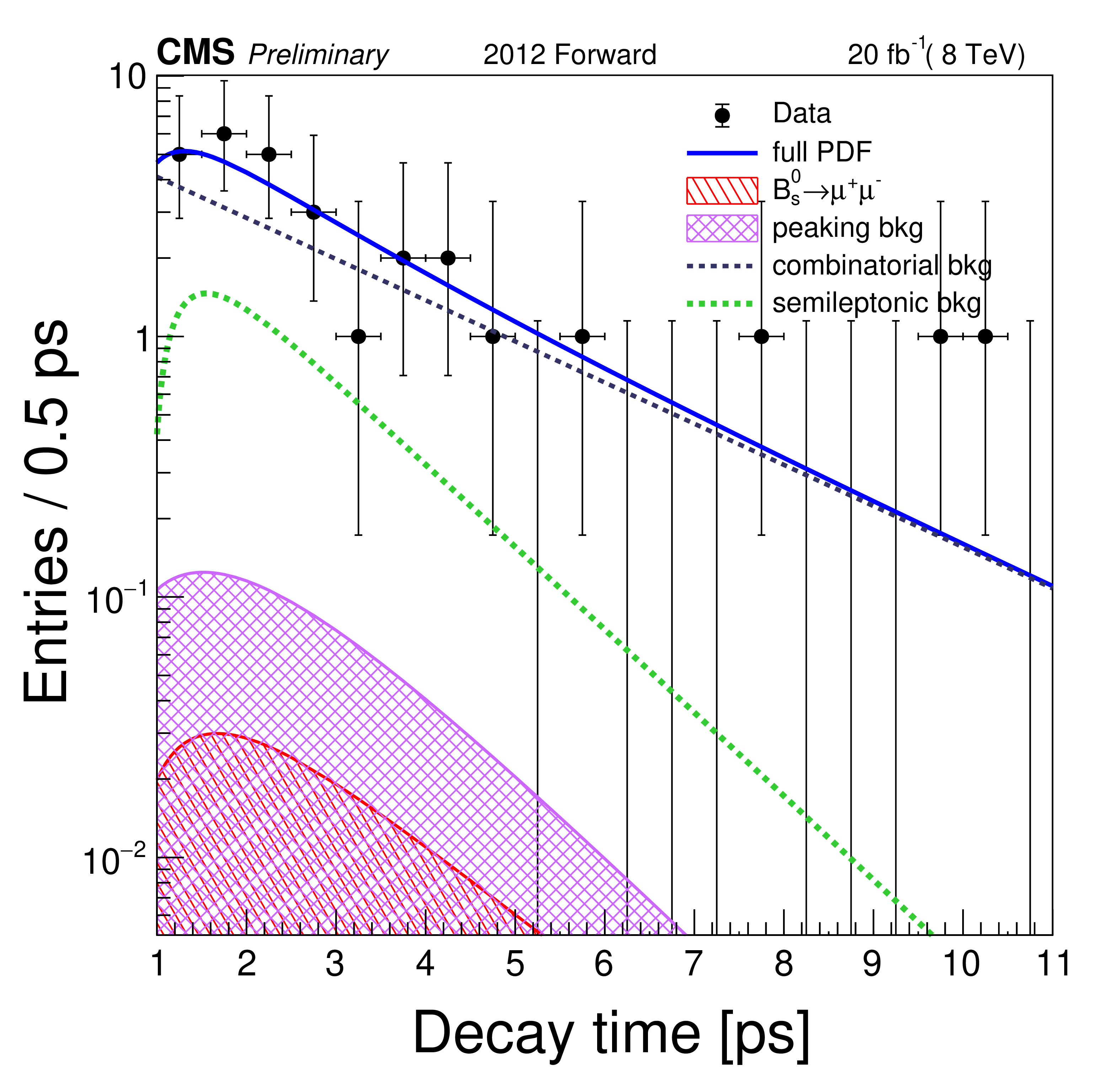
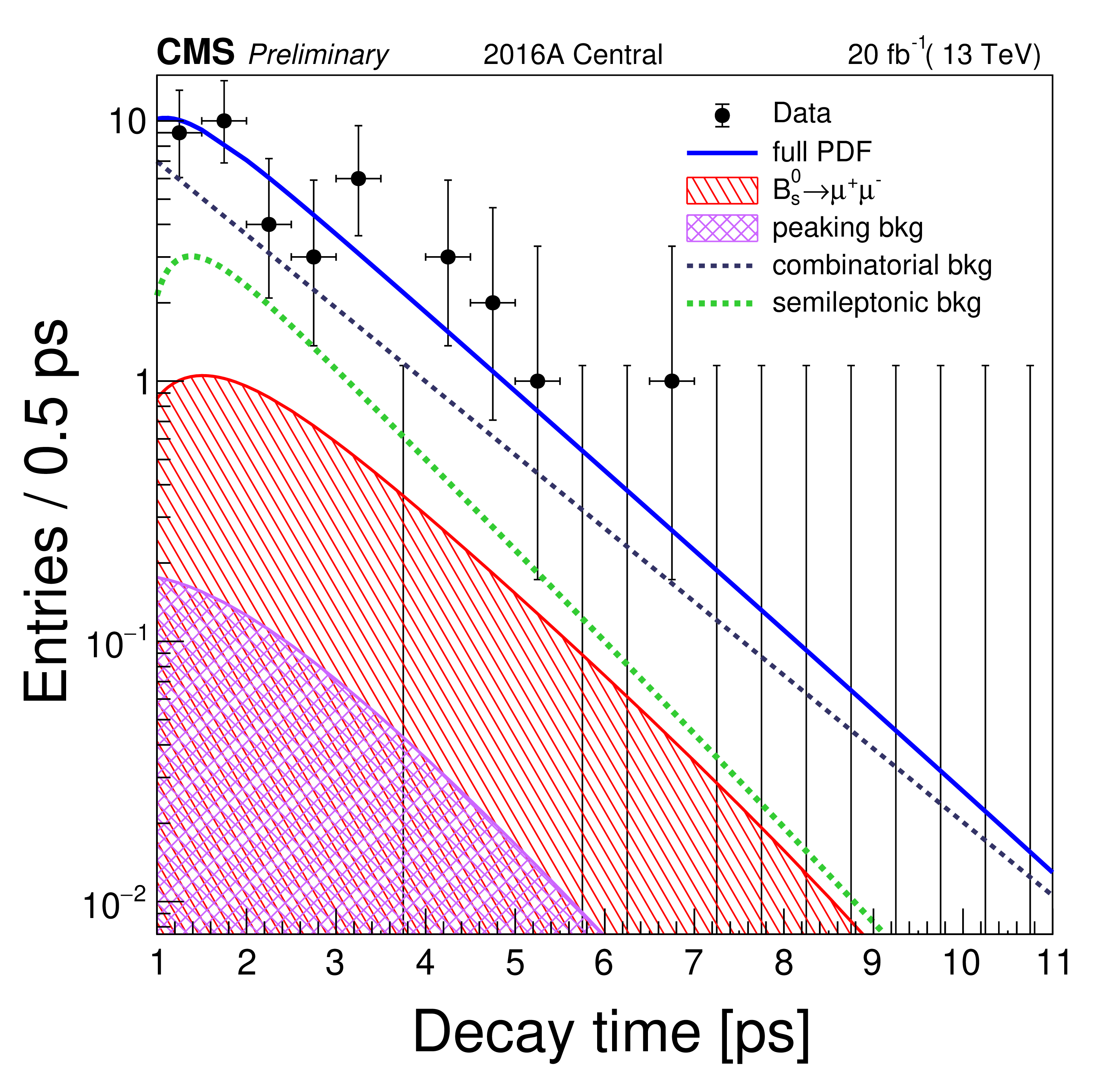
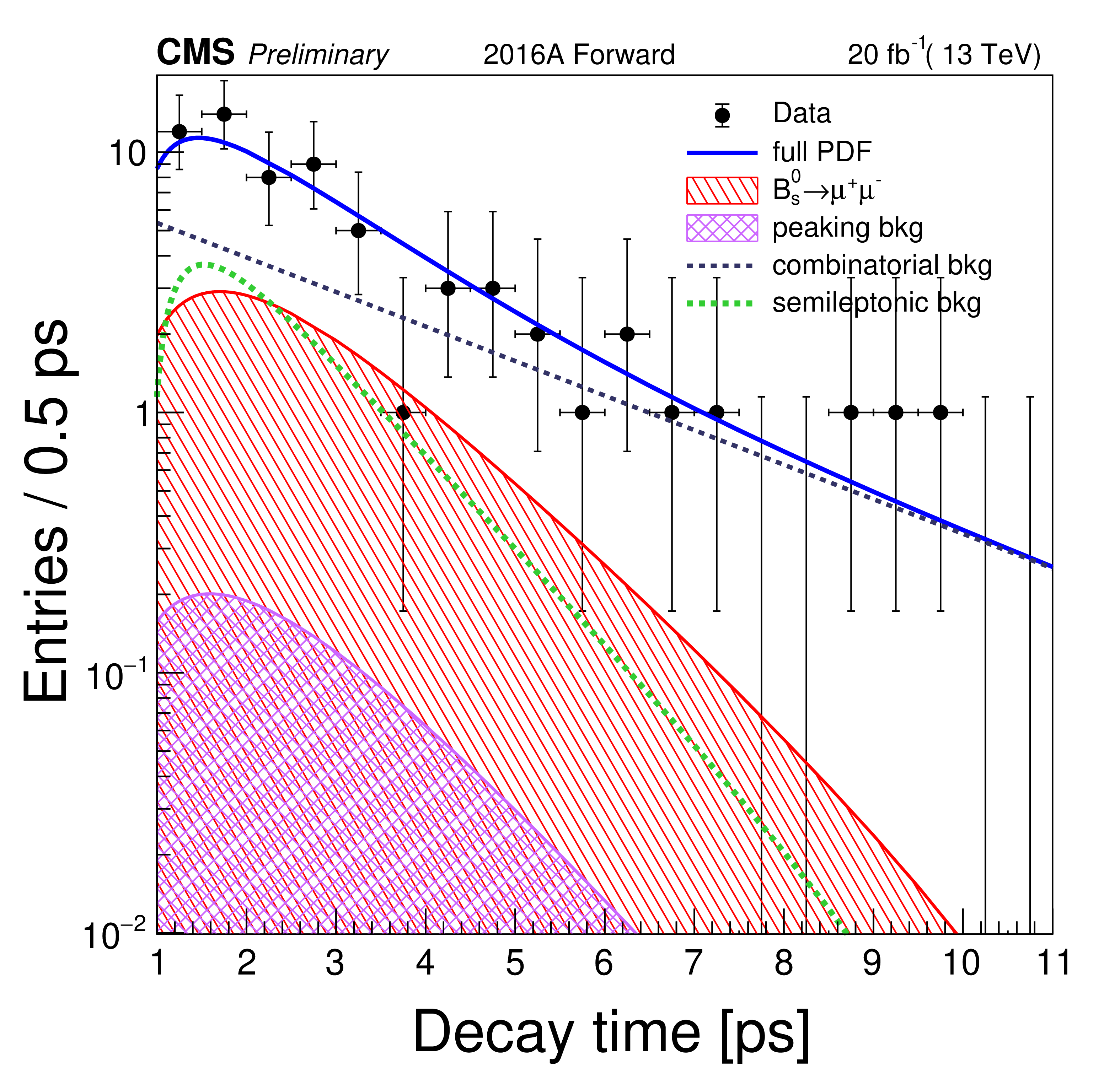
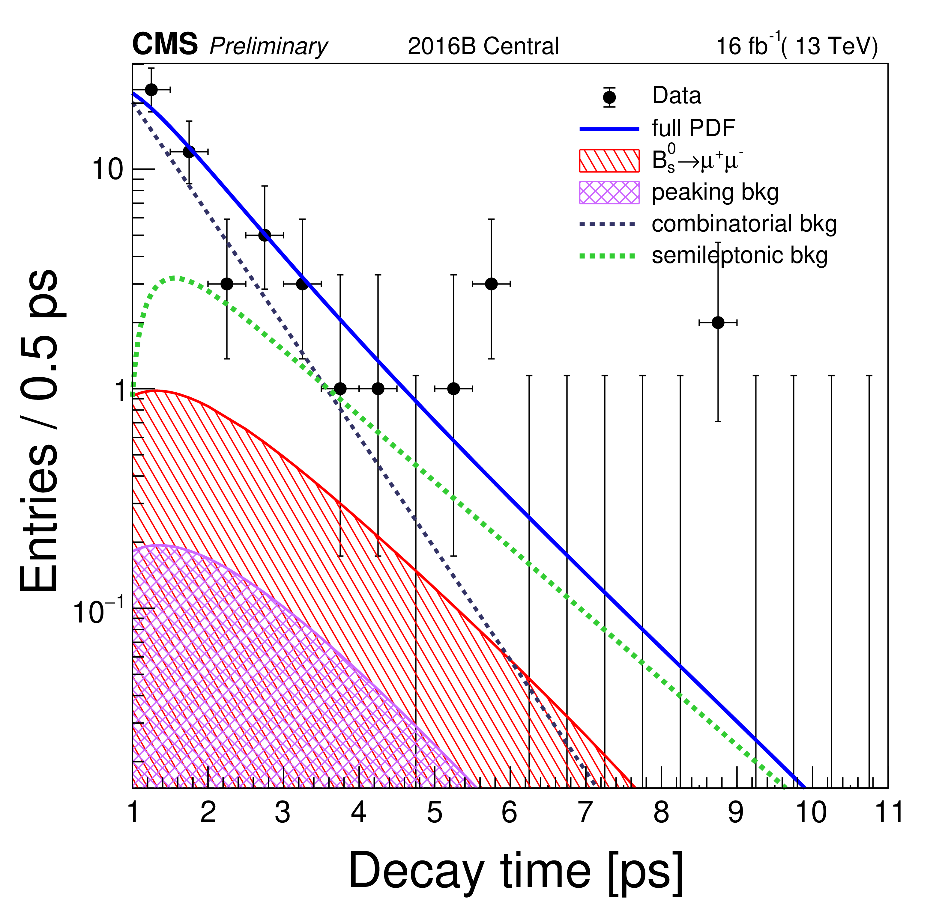
Figure 7:
Invariant mass (left) and proper decay time (right) distributions, with the 2D UML fit projections overlayed. The data combine all channels passing the analysis BDT discriminator requirements as given in Table 4. The total fit is shown by the solid line and the different background components by the broken lines and cross-hatched histogram. The signal component is shown by the red single-hatched histogram. |
png pdf |
Figure 7-a:
Invariant mass (left) and proper decay time (right) distributions, with the 2D UML fit projections overlayed. The data combine all channels passing the analysis BDT discriminator requirements as given in Table 4. The total fit is shown by the solid line and the different background components by the broken lines and cross-hatched histogram. The signal component is shown by the red single-hatched histogram. |
png pdf |
Figure 7-b:
Invariant mass (left) and proper decay time (right) distributions, with the 2D UML fit projections overlayed. The data combine all channels passing the analysis BDT discriminator requirements as given in Table 4. The total fit is shown by the solid line and the different background components by the broken lines and cross-hatched histogram. The signal component is shown by the red single-hatched histogram. |
png pdf |
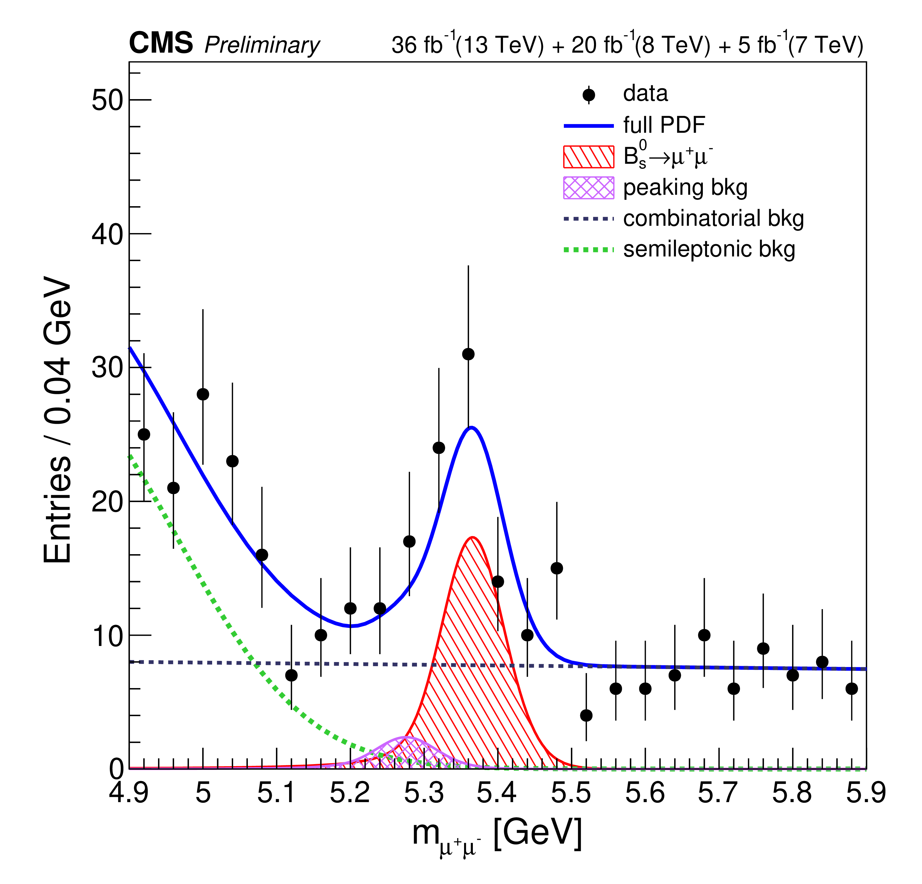
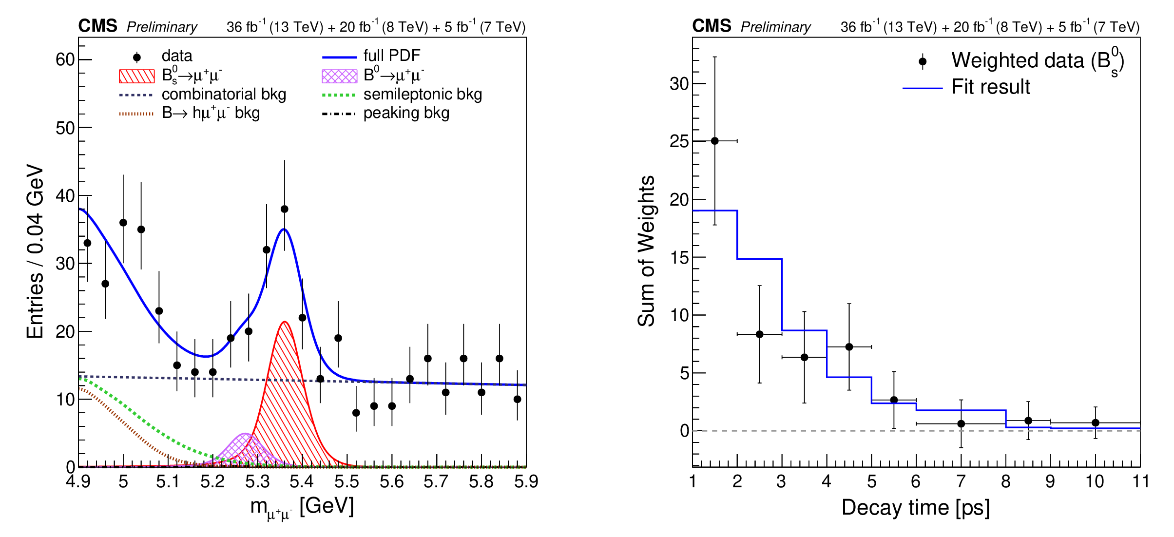
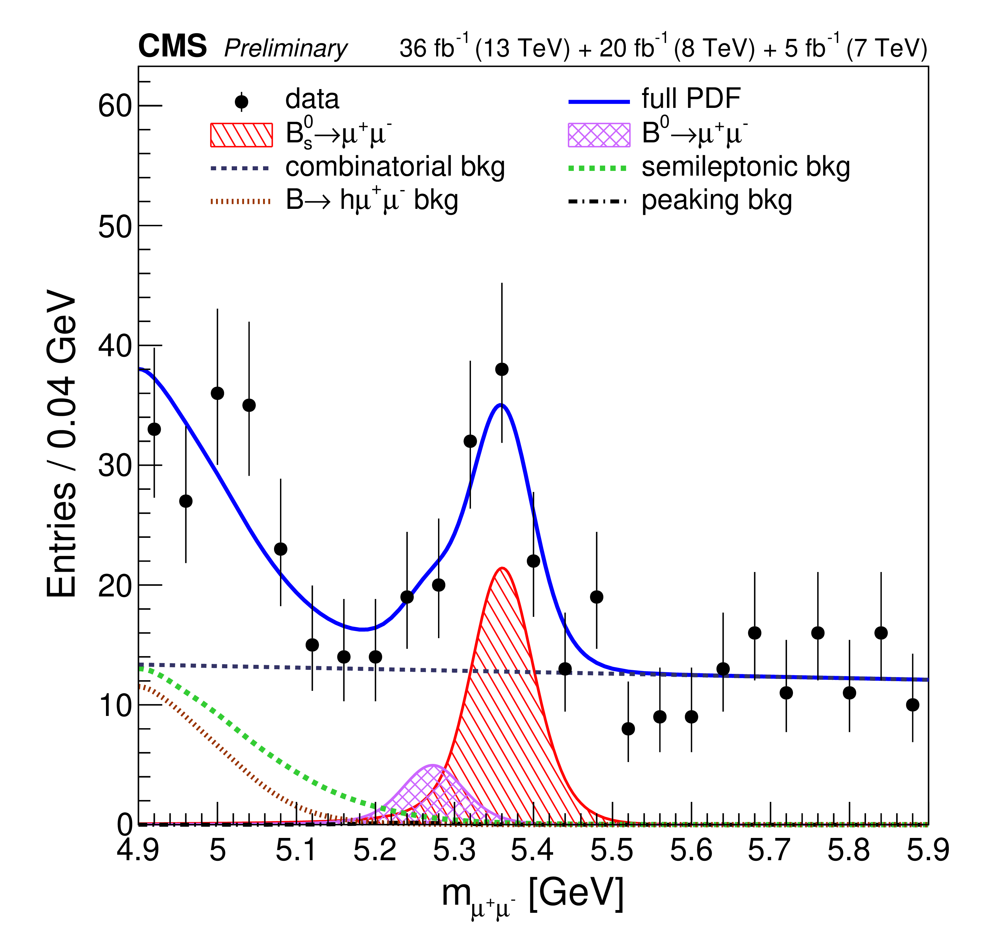
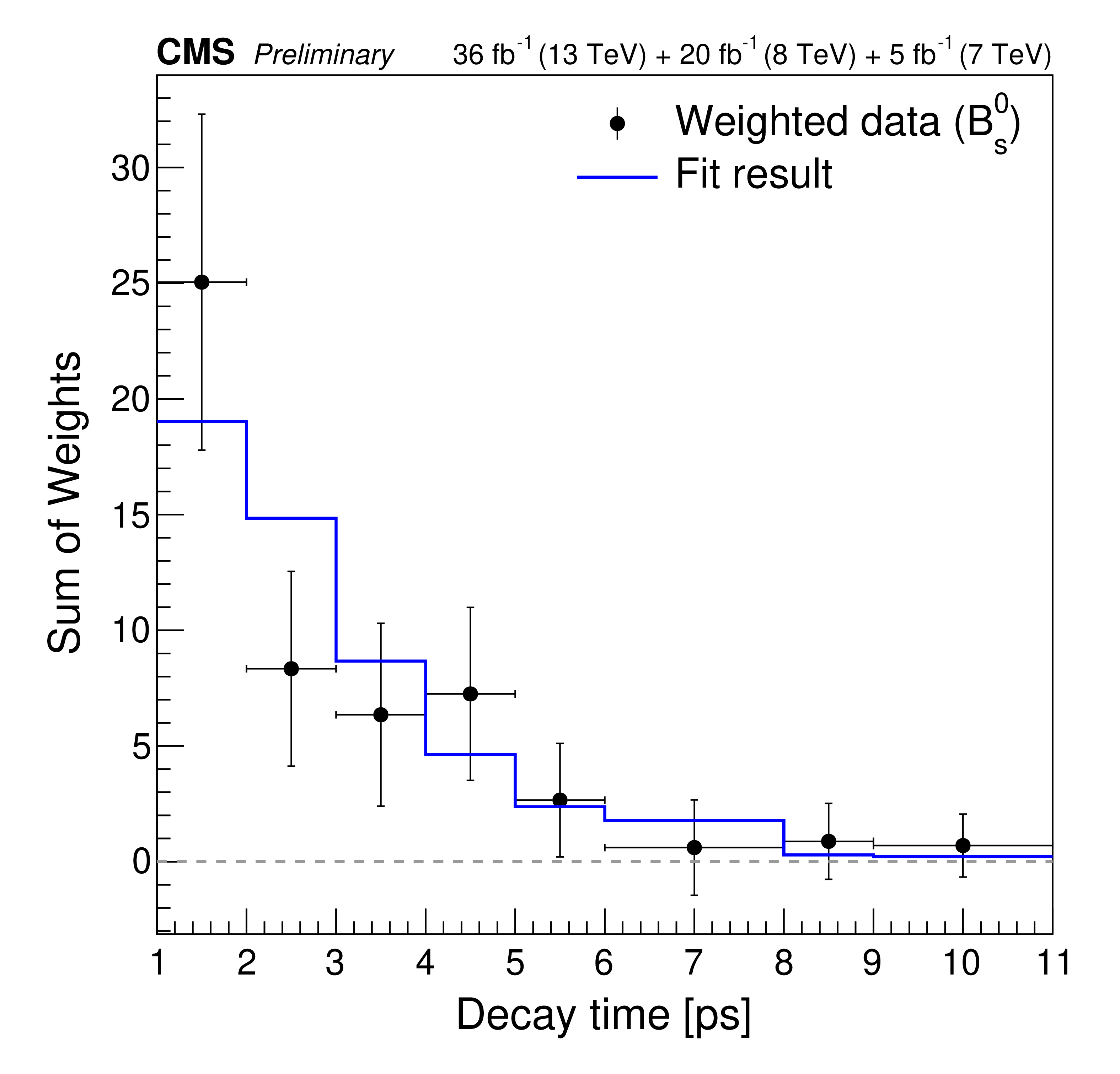
Figure 8:
Invariant mass (left) and proper decay time (right) distributions, with the sPlot fit projections overlayed. The data combine all channels passing the analysis BDT discriminator requirements as given in Table 4. The total fit is shown by the solid line, the different background components by the broken lines and cross-hatched histogram. The signal component is shown by the red single-hatched histogram. |
png pdf |
Figure 8-a:
Invariant mass (left) and proper decay time (right) distributions, with the sPlot fit projections overlayed. The data combine all channels passing the analysis BDT discriminator requirements as given in Table 4. The total fit is shown by the solid line, the different background components by the broken lines and cross-hatched histogram. The signal component is shown by the red single-hatched histogram. |
png pdf |
Figure 8-b:
Invariant mass (left) and proper decay time (right) distributions, with the sPlot fit projections overlayed. The data combine all channels passing the analysis BDT discriminator requirements as given in Table 4. The total fit is shown by the solid line, the different background components by the broken lines and cross-hatched histogram. The signal component is shown by the red single-hatched histogram. |
| Tables | |
png pdf |
Table 1:
Analysis BDT discriminator boundaries per category, channel, and era for the branching fraction determination (2011 has only one category because of the small sample size). These requirements are illustrated in Fig. 4 (bottom row). |
png pdf |
Table 2:
Summary of systematic uncertainty sources described in the text. The uncertainties quoted for the branching fraction $ {{\cal B}}({\mathrm{B}^{0}s \to \mu^{+} \mu^{-}})$ are relative uncertainties, while the uncertainties for the effective lifetime $ {\tau _{\mu^{+} \mu^{-}}}$ are absolute. The relative uncertainties for the upper limit on $ {{\cal B}}({\mathrm{B}^{0} \to \mu^{+} \mu^{-}})$ differ for the background yields, but have negligible impact on that result. The bottom rows provide the total systematic uncertainty and the total uncertainty in the branching fraction and the effective lifetime measurements. (*) indicates that the contribution is included in other items. |
png pdf |
Table 3:
Summary of the fitted yields (for ${\mathrm{B}^{0}s \to \mu^{+} \mu^{-}}$, ${\mathrm{B}^{0} \to \mu^{+} \mu^{-}}$, the combinatorial background for 4.9 $ < {m_{\mu^{+} \mu^{-}}} < $ 5.9 GeV, and the ${\mathrm{B^{+}} \to {\mathrm{J}/\psi} \mathrm{K^{+}}} $ normalization), the average ${{p_{\text {T}}}}$ of the ${\mathrm{B}^{0}s \to \mu^{+} \mu^{-}} $ signal, and the ratio of efficiencies between the normalization and the signal in all 14 categories of the 3D UML branching fraction fit. The high and low ranges of the analysis BDT discriminator distribution are defined in Table 1. The size of peaking background is approximately 5-10% of the ${\mathrm{B}^{0} \to \mu^{+} \mu^{-}}$ signal. The average ${{p_{\text {T}}}}$ is calculated from the MC simulation and has negligible uncertainties. The uncertainties shown include the statistical and systematic components. It should be noted that the ${\mathrm{B}^{0}s \to \mu^{+} \mu^{-}} $ and ${\mathrm{B}^{0} \to \mu^{+} \mu^{-}}$ yield uncertainties are determined from the branching fraction fit and also include the normalization uncertainties. |

png pdf |
Table 4:
Analysis BDT discriminator minimum requirements per channel and era for the 1D and 2D effective lifetime fits. |
| Summary |
| Measurements of the rare leptonic B meson decays ${\mathrm{B}^{0}_{s}\to\mu^{+}\mu^{-}} $ and ${\mathrm{B}^{0}\to\mu^{+}\mu^{-}} $ have been performed in pp collision data collected by the CMS experiment at the LHC, corresponding to a combined data sample of 5 fb$^{-1}$ at center-of-mass energy 7 TeV, 20 fb$^{-1}$ at 8 TeV, and 36 fb$^{-1}$ at 13 TeV. The ${\mathrm{B}^{0}_{s}\to\mu^{+}\mu^{-}} $ decay is observed with a significance of 5.6 standard deviations and the time-integrated branching fraction is measured to be ${\cal B}({\rm B_s^0}\to\mu^+\mu^-) =$ [2.9$^{+0.7}_{-0.6}$ (exp) $\pm$ 0.2 (frag)] $\times10^{-9}$, where the first uncertainty combines the statistical and systematic terms. No significant ${\rm B^0}\to\mu^+\mu^-$ signal is observed and an upper limit ${\cal B}({\rm B^0}\to\mu^+\mu^-) < 3.6\times10^{-10}$ is determined at 95% confidence level. The ${\mathrm{B}^{0}_{s}\to\mu^{+}\mu^{-}} $ effective lifetime, measured for the first time by the CMS experiment, is found to be $\tau_{\mu^+\mu^-} = $ 1.70$^{+0.61}_{-0.44}$ ps, where the uncertainty combines both statistical and systematic components. The results for the branching fractions supersede the previous results from CMS [5], which were based on the 7 and 8 TeV data only. All results are in agreement with the standard model predictions. |
| Additional Figures | |
png pdf |
Additional Figure 1:
(Left) The two-dimensional probability contours representing the simultaneous measurement of the relative probabilities of the $\mathrm{B_s}^{0}\to \mu ^+\mu ^-$ vs. $\mathrm{B}^{0}\to \mu ^+\mu ^-$ decays; the various contours correspond to (innermost to outermost) 1, 2, 3, 4, and 5 standard deviations. The black cross represents the CMS measurement, while the red point corresponds to the SM prediction. (Right) Confidence level (CL) as a function of the assumed $\mathrm{B}^{0}\to \mu ^+\mu ^-$ branching fraction. The blue solid curve shows the values calculated with a likelihood scan which is based on Wilks' theorem, while the red dashed curve show the results from the Feldman-Cousins approach. |
png pdf |
Additional Figure 1b:
Confidence level (CL) as a function of the assumed $\mathrm{B}^{0}\to \mu ^+\mu ^-$ branching fraction. The blue solid curve shows the values calculated with a likelihood scan which is based on Wilks' theorem, while the red dashed curve show the results from the Feldman-Cousins approach. |
png pdf |
Additional Figure 1-b:
(Left) The two-dimensional probability contours representing the simultaneous measurement of the relative probabilities of the $\mathrm{B_s}^{0}\to \mu ^+\mu ^-$ vs. $\mathrm{B}^{0}\to \mu ^+\mu ^-$ decays; the various contours correspond to (innermost to outermost) 1, 2, 3, 4, and 5 standard deviations. The black cross represents the CMS measurement, while the red point corresponds to the SM prediction. (Right) Confidence level (CL) as a function of the assumed $\mathrm{B}^{0}\to \mu ^+\mu ^-$ branching fraction. The blue solid curve shows the values calculated with a likelihood scan which is based on Wilks' theorem, while the red dashed curve show the results from the Feldman-Cousins approach. |
png pdf |
Additional Figure 2:
The one-dimensional likelihood ratio ($-2\ln(L/L_{\rm max})$) as functions of the assumed $\mathrm{B_s}^{0}\to \mu ^+\mu ^-$ (left) or $\mathrm{B}^{0}\to \mu ^+\mu ^-$ (right) branching fractions, when the other branching fraction is profiled together with other nuisance parameters. |
png pdf |
Additional Figure 2-a:
The one-dimensional likelihood ratio ($-2\ln(L/L_{\rm max})$) as functions of the assumed $\mathrm{B_s}^{0}\to \mu ^+\mu ^-$ branching fraction, when the $\mathrm{B}^{0}\to \mu ^+\mu ^-$ branching fraction is profiled together with other nuisance parameters. |
png pdf |
Additional Figure 2-b:
The one-dimensional likelihood ratio ($-2\ln(L/L_{\rm max})$) as functions of the assumed $\mathrm{B}^{0}\to \mu ^+\mu ^-$ branching fraction, when the $\mathrm{B_s}^{0}\to \mu ^+\mu ^-$ branching fraction is profiled together with other nuisance parameters. |

png pdf |
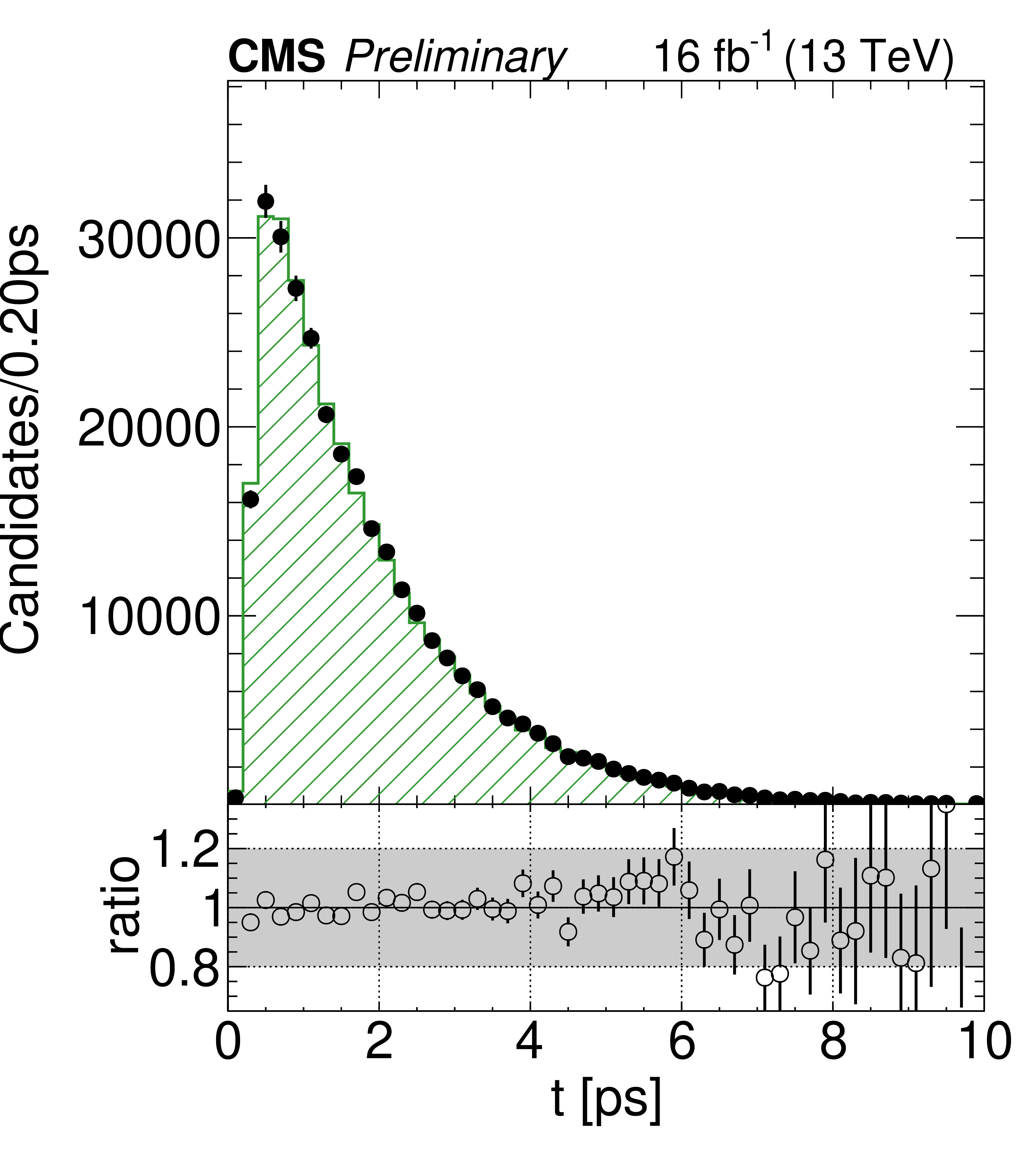
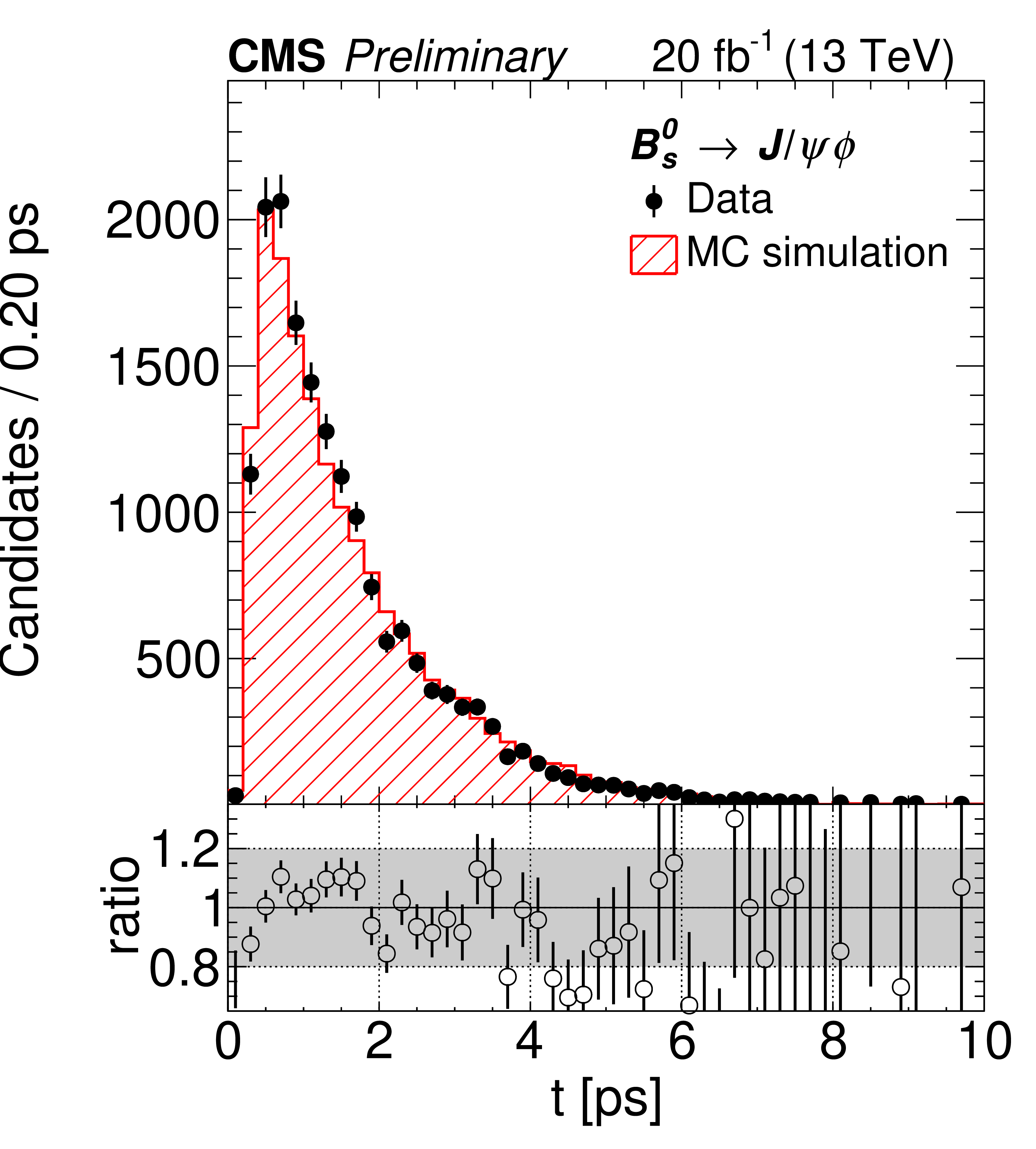
Additional Figure 3:
The lifetime distributions of the observed $\mathrm{B_s}^{0}\to \mu ^+\mu ^-$ candidates, fitted with a function that has the exponential shape expected for the lifetime of a particle. The plot on the left shows all of the candidates; the plot in the middle shows the candidates in the signal region of $m_{\mu ^+\mu ^-}$; the plot on the right shows the distribution after a subtraction of the background contributions. The data in the left-hand histogram are plotted on a logarithmic scale, while the middle and right-hand histograms are plotted using a linear scale. The turnover of the function at very low lifetimes is an artifact of a selection requirement on the minimum decay length of the $\mathrm{B_s}^{0}$ meson. |
png pdf |
Additional Figure 3-a:
The lifetime distribution of the observed $\mathrm{B_s}^{0}\to \mu ^+\mu ^-$ candidates, fitted with a function that has the exponential shape expected for the lifetime of a particle. The plot shows all of the candidates. The data are plotted using a logarithmic scale. The turnover of the function at very low lifetimes is an artifact of a selection requirement on the minimum decay length of the $\mathrm{B_s}^{0}$ meson. |
png pdf |
Additional Figure 3-b:
The lifetime distribution of the observed $\mathrm{B_s}^{0}\to \mu ^+\mu ^-$ candidates, fitted with a function that has the exponential shape expected for the lifetime of a particle. The plot shows the candidates in the signal region of $m_{\mu ^+\mu ^-}$. The data are plotted using a linear scale. The turnover of the function at very low lifetimes is an artifact of a selection requirement on the minimum decay length of the $\mathrm{B_s}^{0}$ meson. |
png pdf |
Additional Figure 3-c:
The lifetime distribution of the observed $\mathrm{B_s}^{0}\to \mu ^+\mu ^-$ candidates, fitted with a function that has the exponential shape expected for the lifetime of a particle. The plot shows the distribution after a subtraction of the background contributions. The data are plotted using a linear scale. The turnover of the function at very low lifetimes is an artifact of a selection requirement on the minimum decay length of the $\mathrm{B_s}^{0}$ meson. |
png pdf |
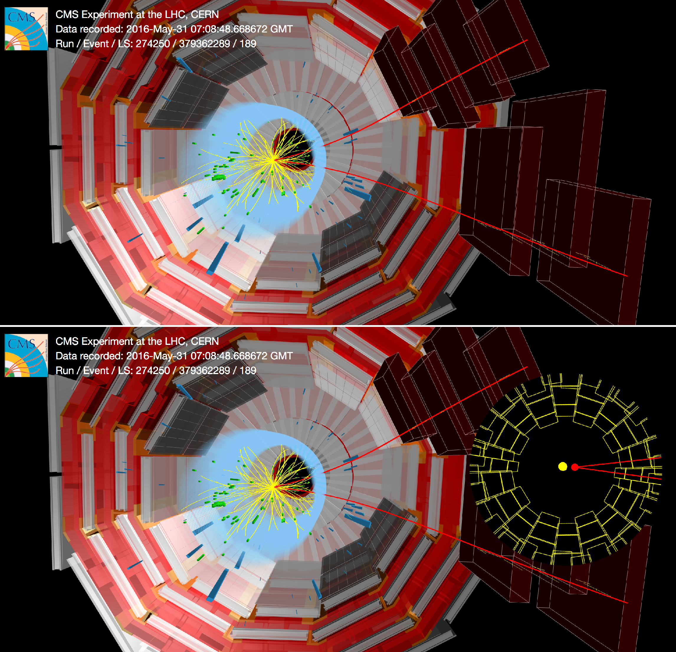
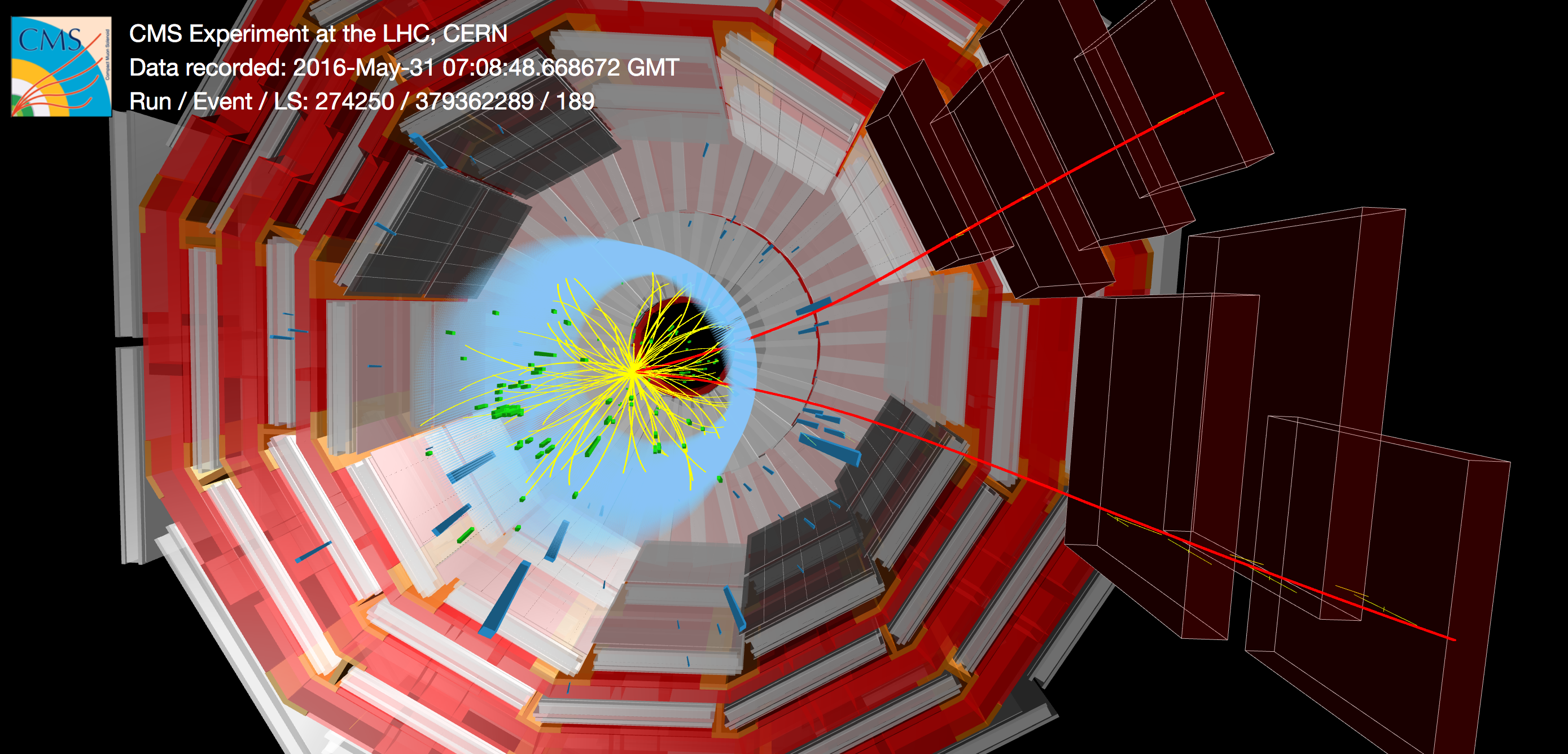
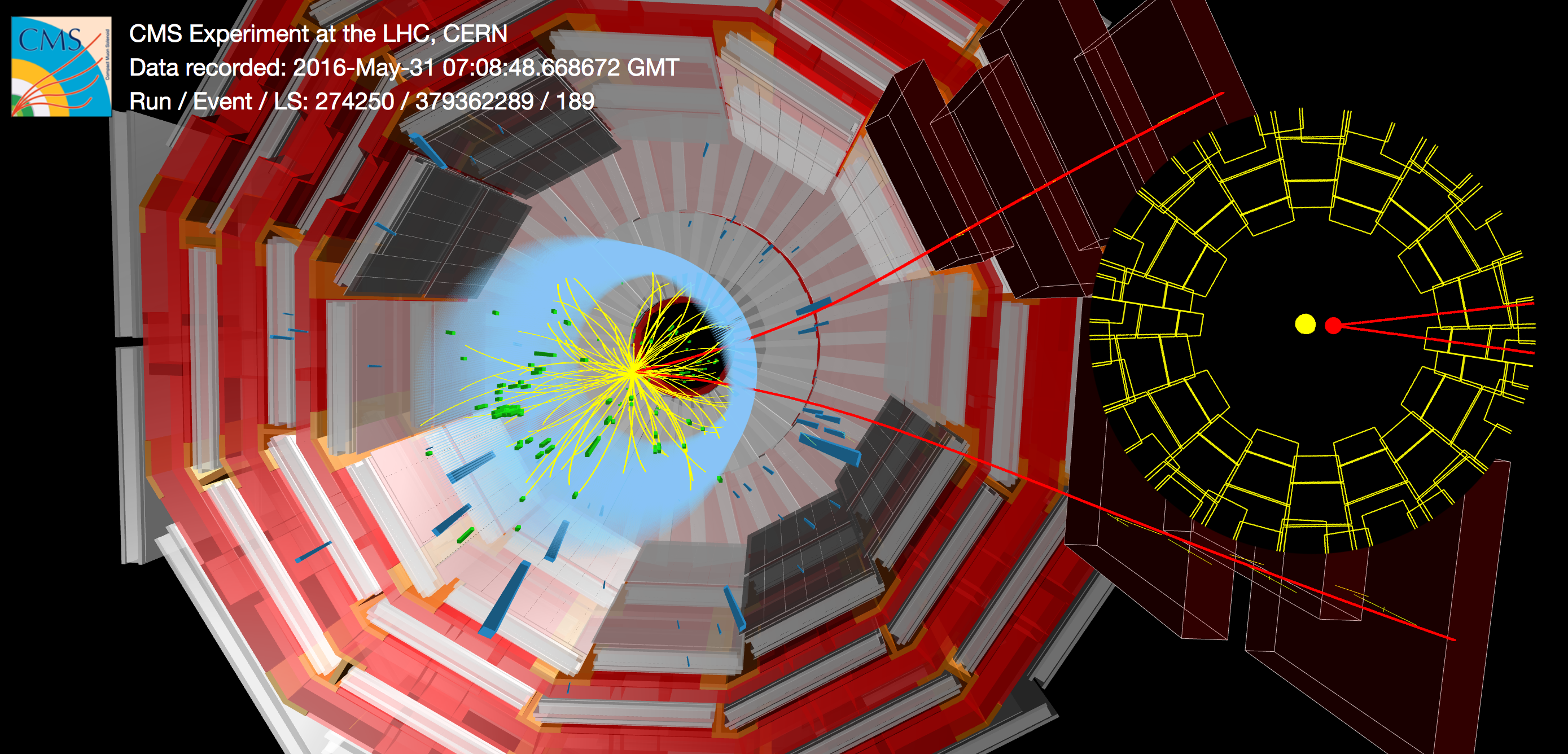
Additional Figure 4:
Event displays of a $\mathrm{B_s}^{0}\to \mu ^+\mu ^-$ candidate in Run 2 data. The two curved red lines correspond to the two muons from the decay. The inset zooms in on the innermost CMS detector region. The tracks other than the muon ones have been removed for clarity. The two muons do not come from the proton-proton collision point, shown as a yellow dot, but from the decay vertex of the $\mathrm{B_s}^{0}$ meson, shown as a red dot. |
png |
Additional Figure 4-a:
Event displays of a $\mathrm{B_s}^{0}\to \mu ^+\mu ^-$ candidate in Run 2 data. The two curved red lines correspond to the two muons from the decay. The inset zooms in on the innermost CMS detector region. The tracks other than the muon ones have been removed for clarity. The two muons do not come from the proton-proton collision point, shown as a yellow dot, but from the decay vertex of the $\mathrm{B_s}^{0}$ meson, shown as a red dot. |
png |
Additional Figure 4-b:
Event displays of a $\mathrm{B_s}^{0}\to \mu ^+\mu ^-$ candidate in Run 2 data. The two curved red lines correspond to the two muons from the decay. The inset zooms in on the innermost CMS detector region. The tracks other than the muon ones have been removed for clarity. The two muons do not come from the proton-proton collision point, shown as a yellow dot, but from the decay vertex of the $\mathrm{B_s}^{0}$ meson, shown as a red dot. |
png pdf |
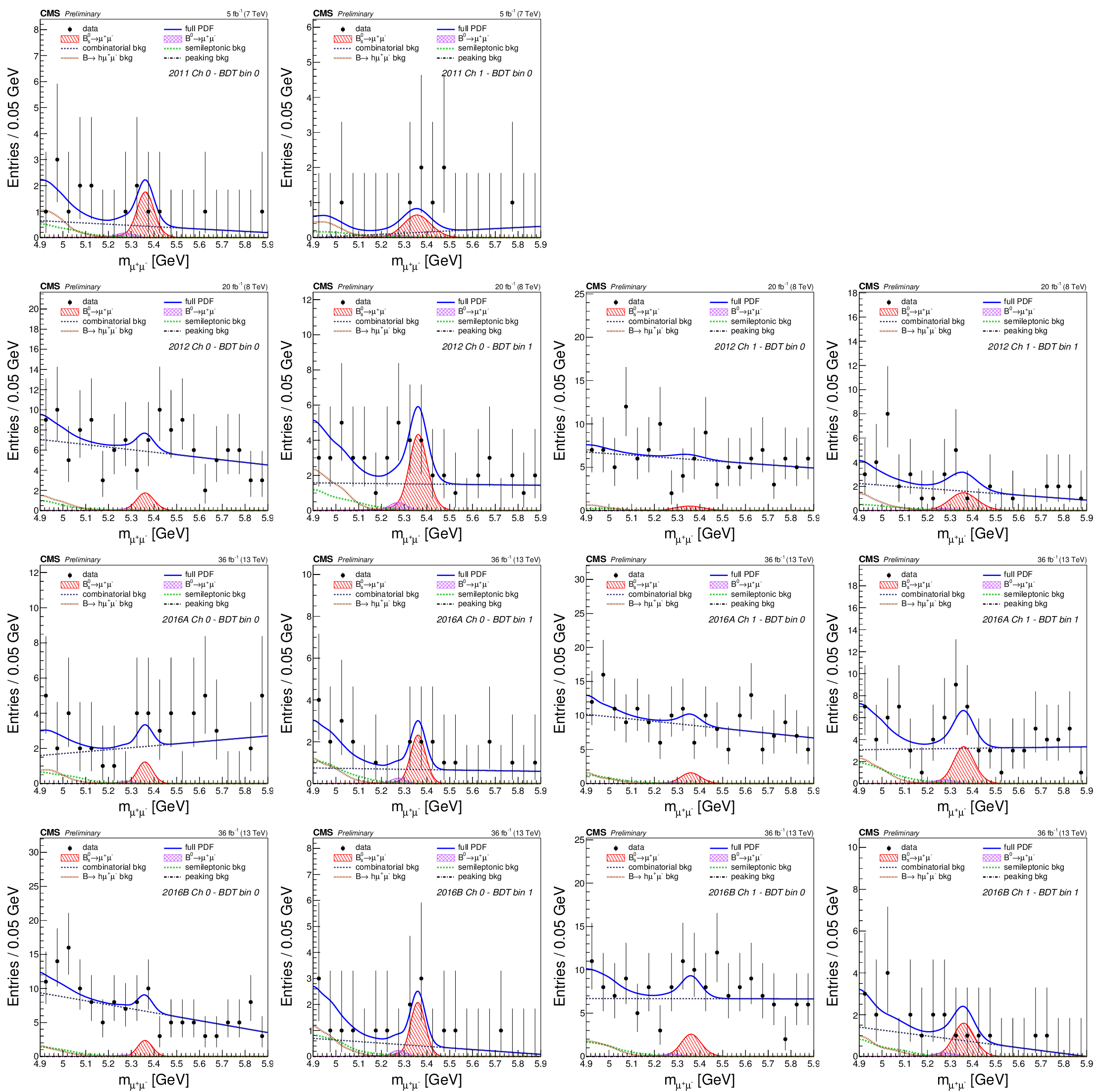
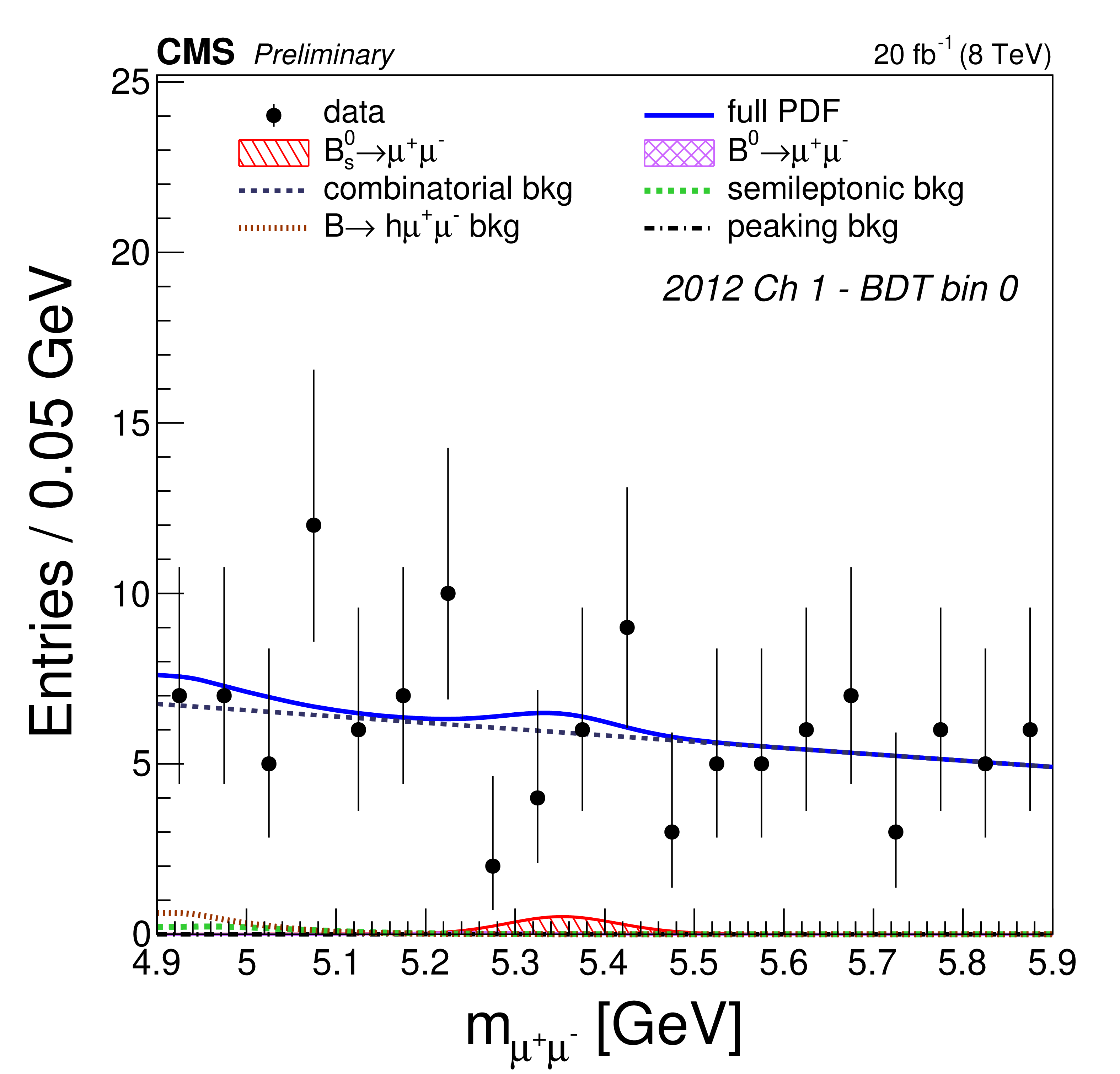
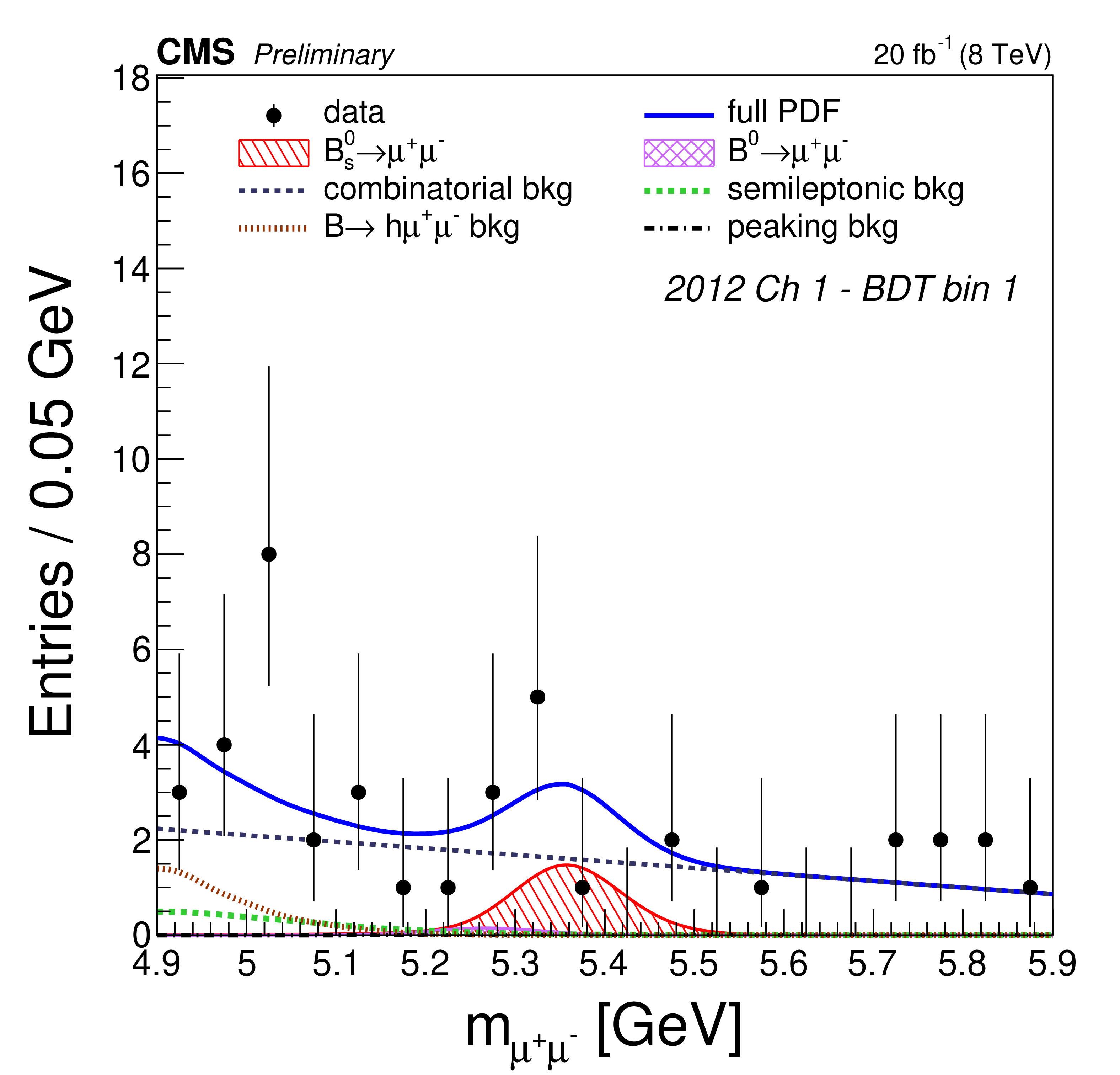
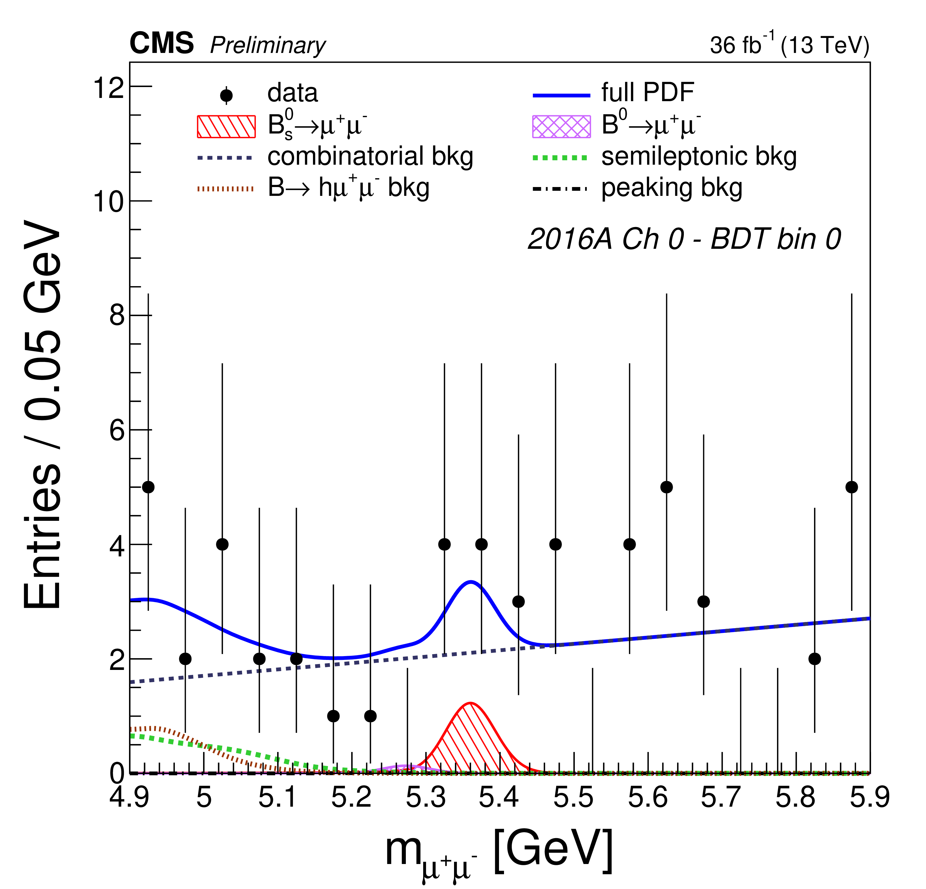
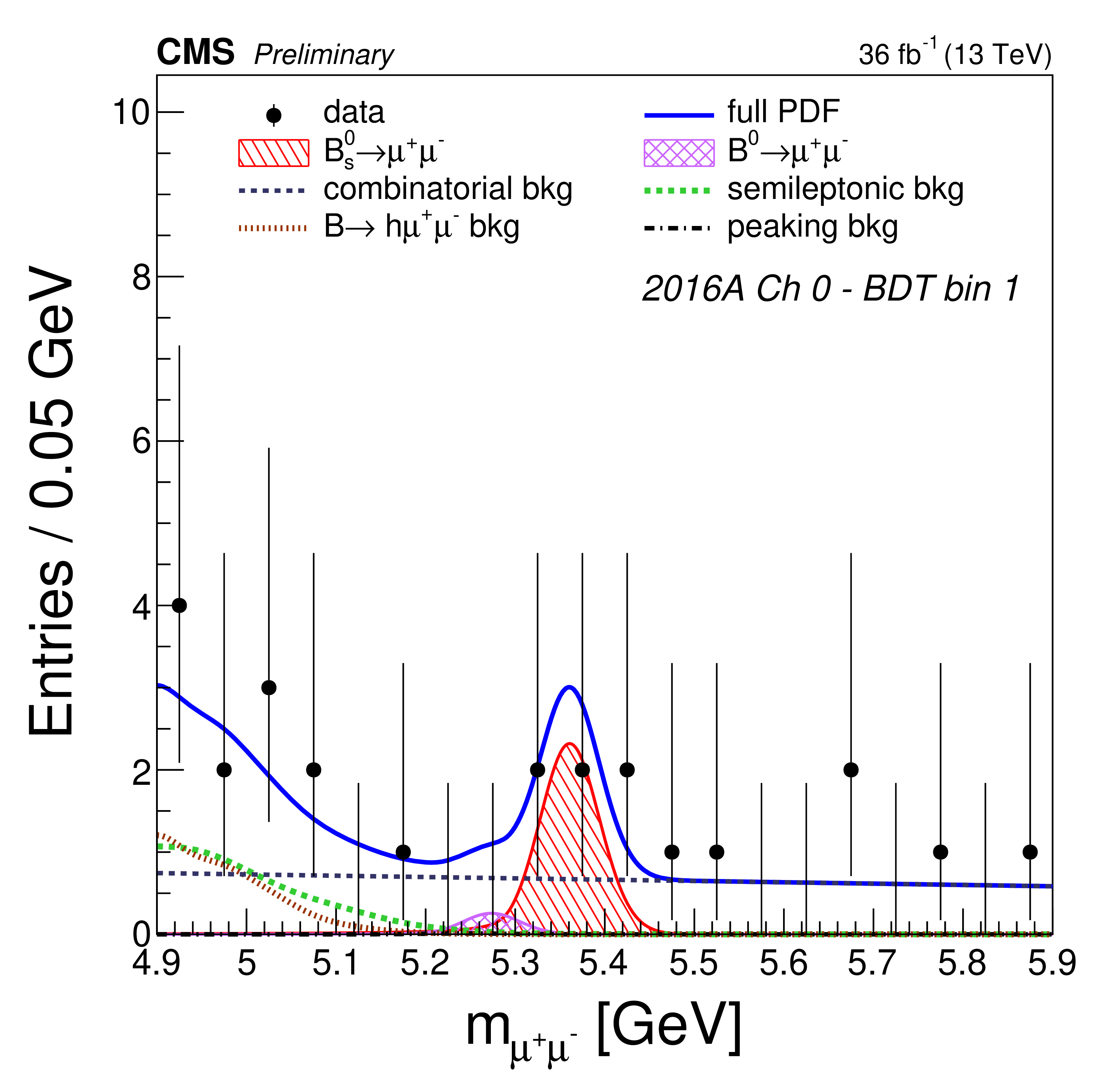
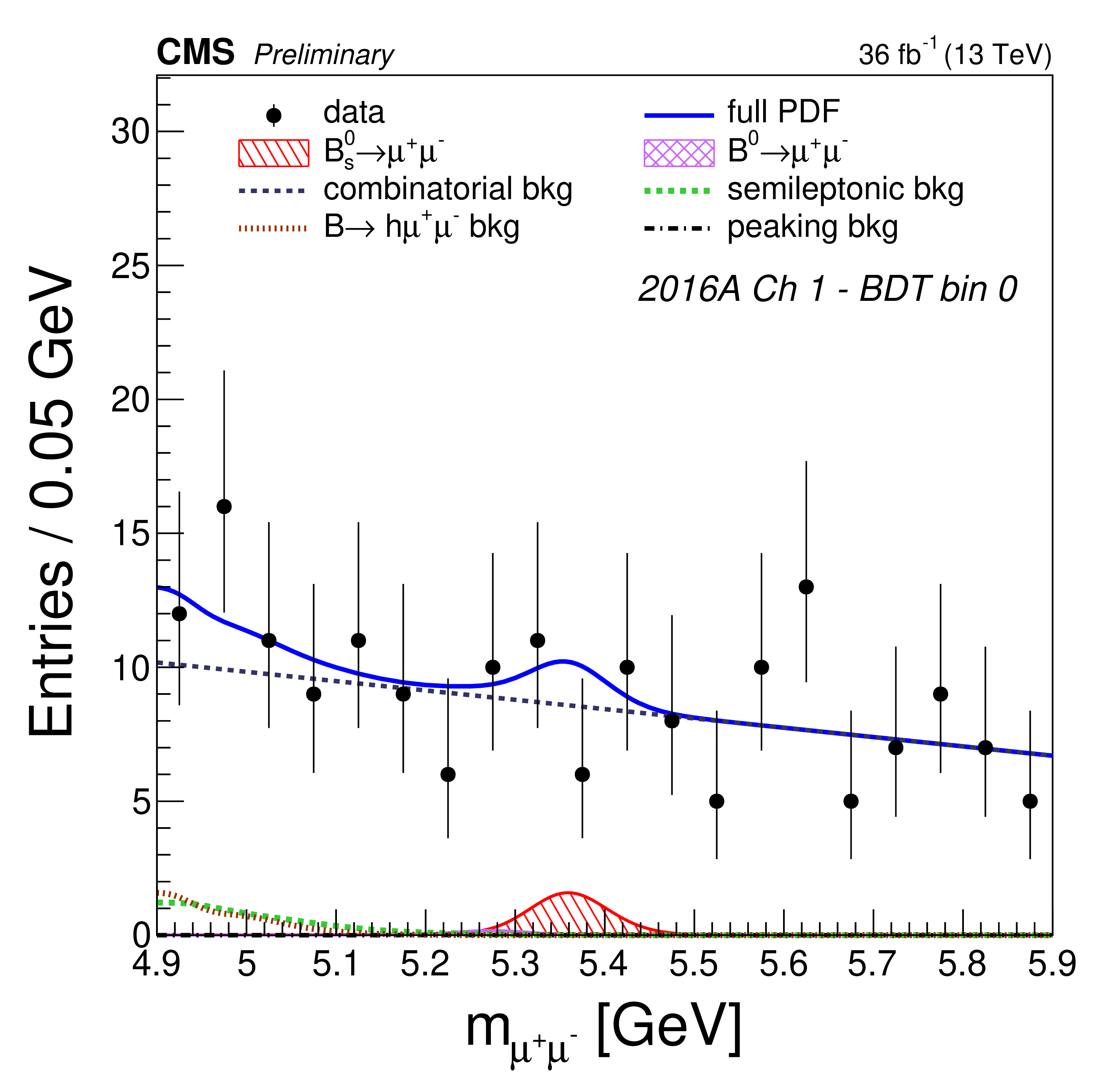
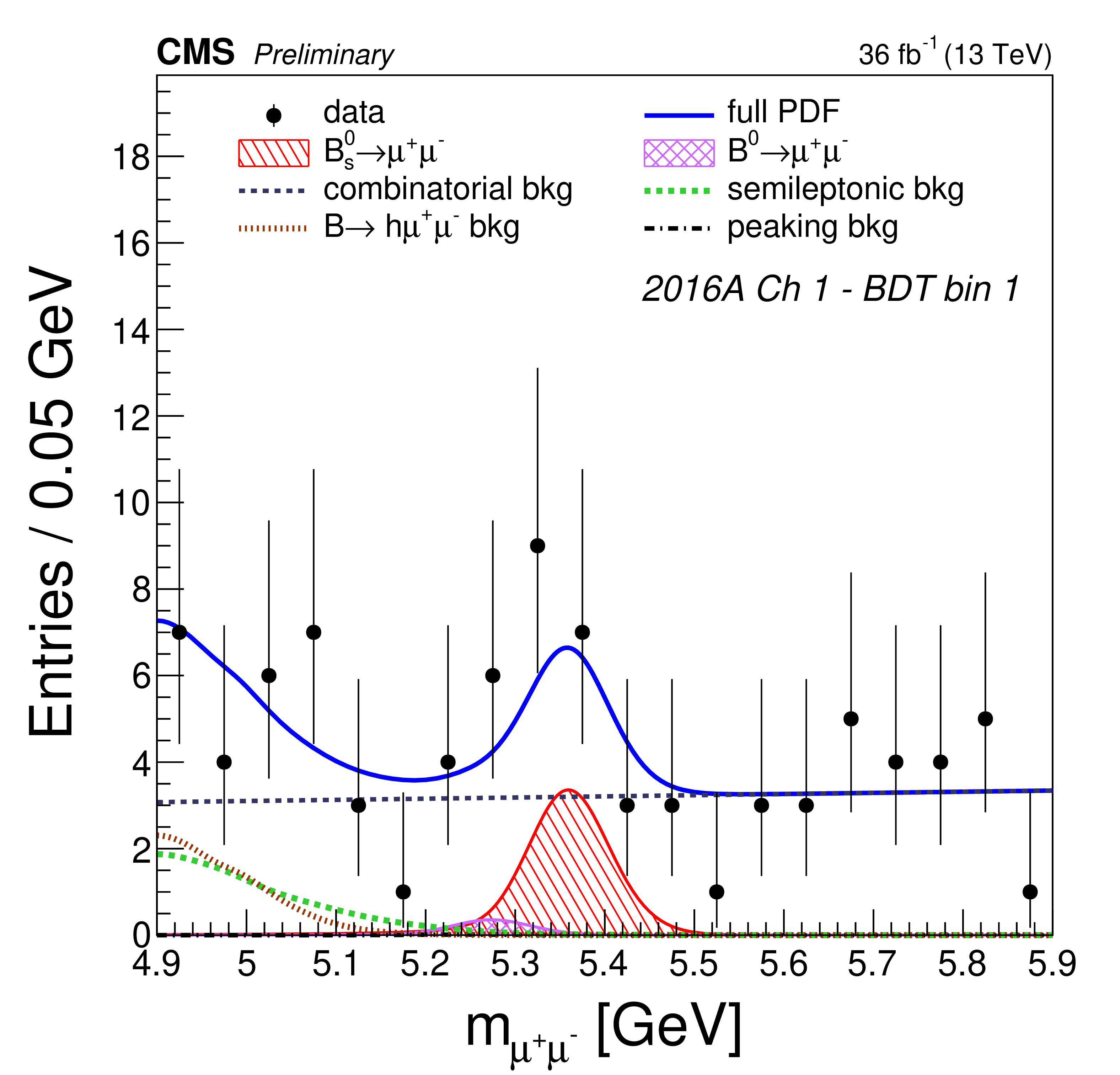
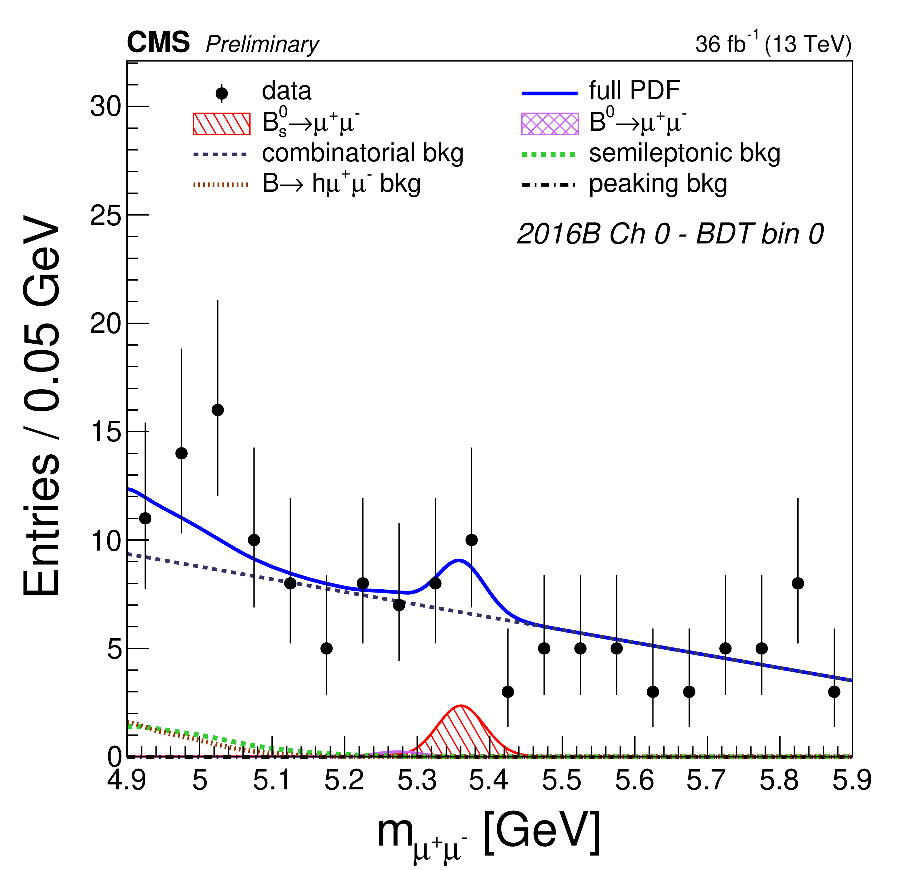
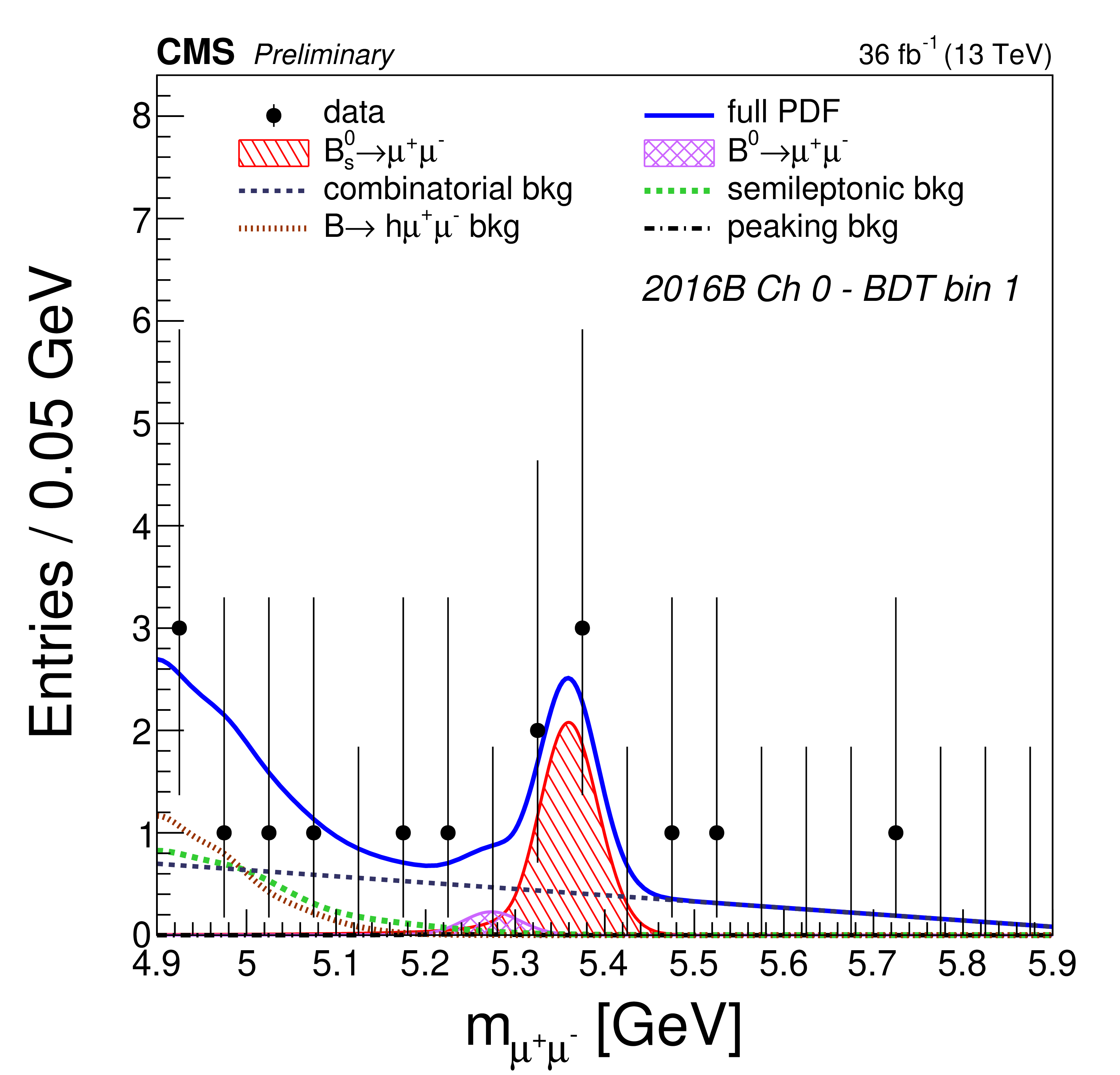
Additional Figure 5:
Invariant mass distribution for each analysis BDT category with the fit projection overlays for the branching fraction results. The total fit is shown by the solid line and the different background components by the broken lines. The signal components are shown by the hatched histograms. |
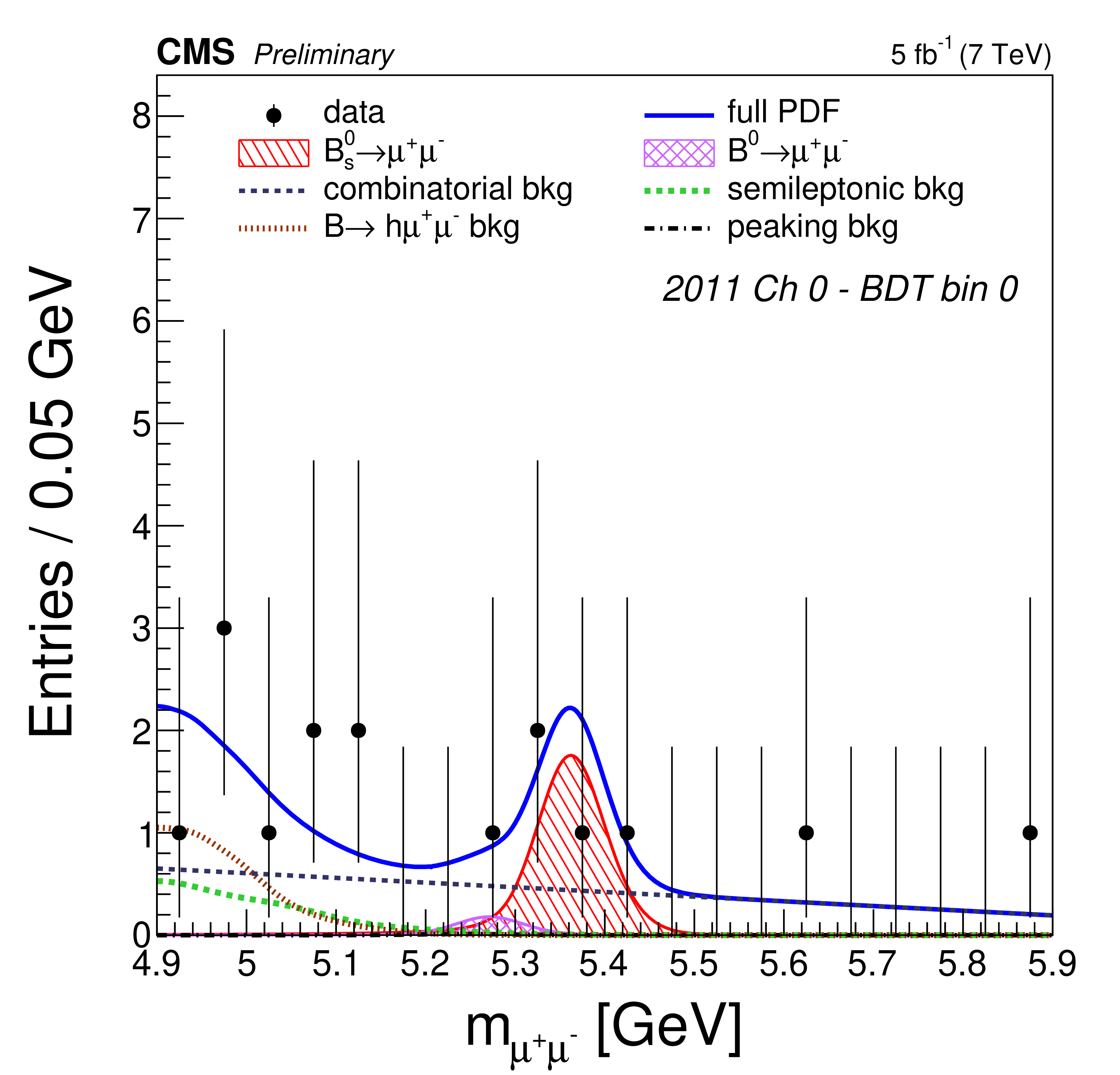
png pdf |
Additional Figure 5-a:
Invariant mass distribution for one of the analysis BDT categories with the fit projection overlays for the branching fraction results. The total fit is shown by the solid line and the different background components by the broken lines. The signal components are shown by the hatched histograms. |
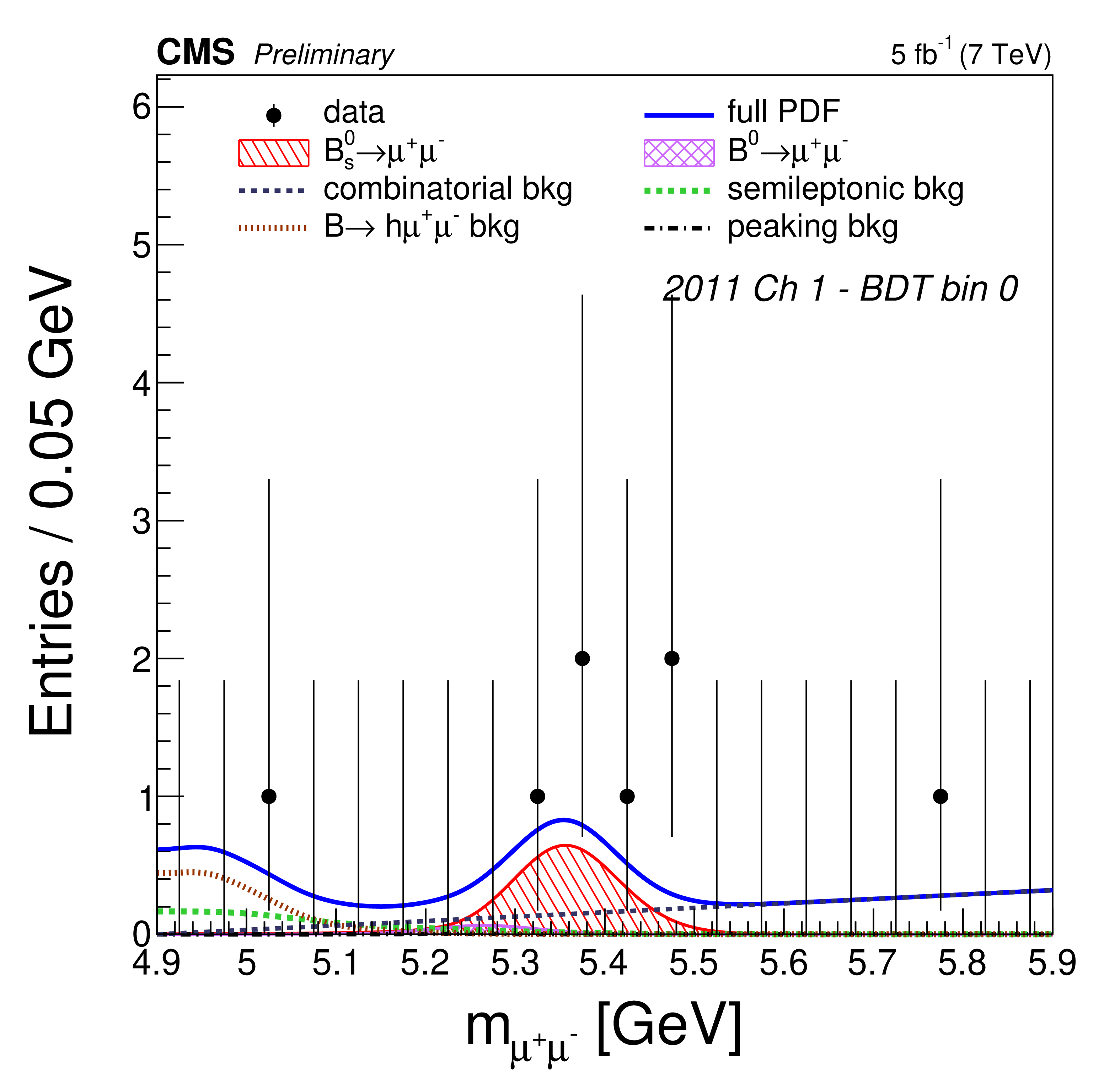
png pdf |
Additional Figure 5-b:
Invariant mass distribution for one of the analysis BDT categories with the fit projection overlays for the branching fraction results. The total fit is shown by the solid line and the different background components by the broken lines. The signal components are shown by the hatched histograms. |
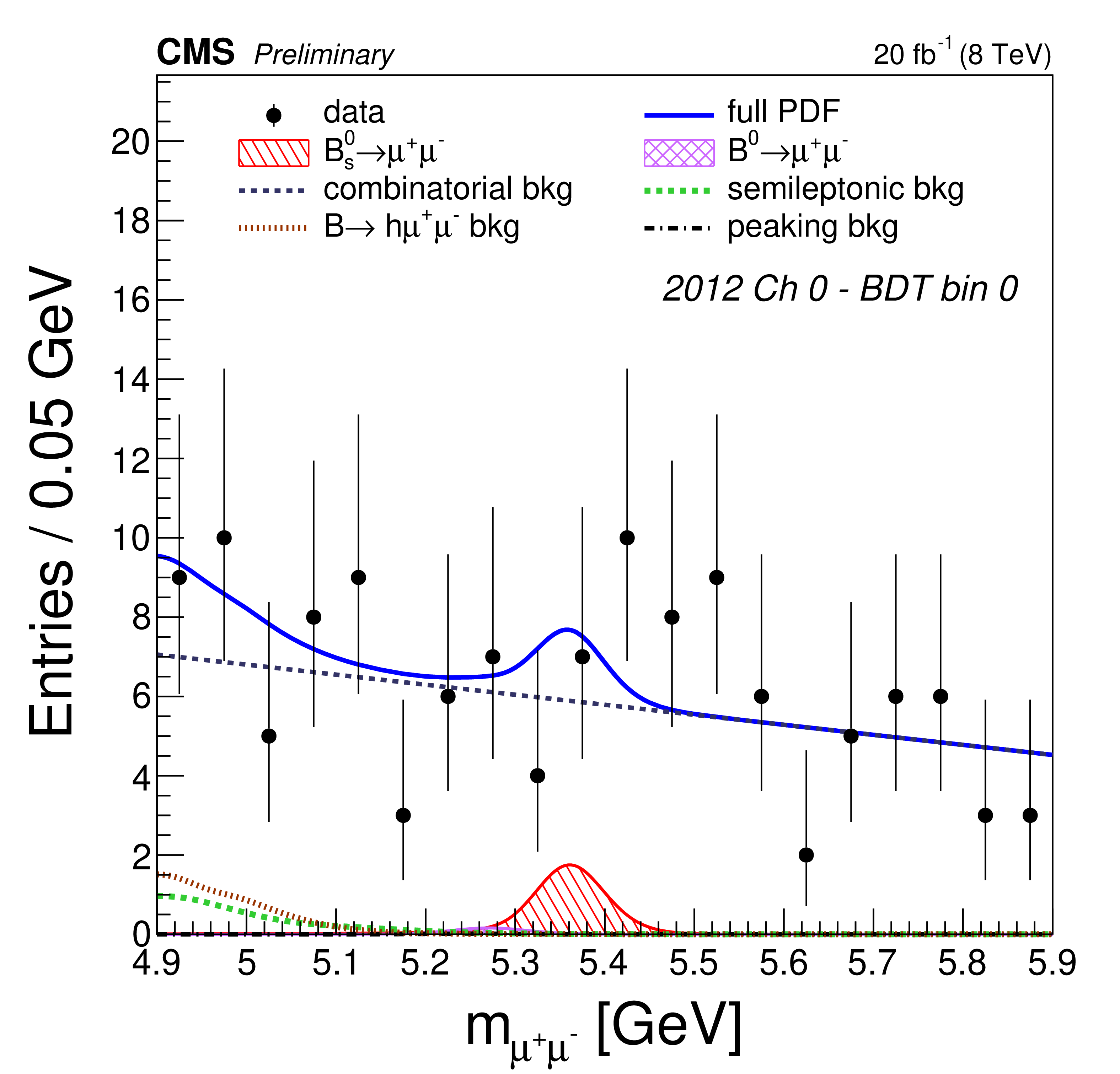
png pdf |
Additional Figure 5-c:
Invariant mass distribution for one of the analysis BDT categories with the fit projection overlays for the branching fraction results. The total fit is shown by the solid line and the different background components by the broken lines. The signal components are shown by the hatched histograms. |
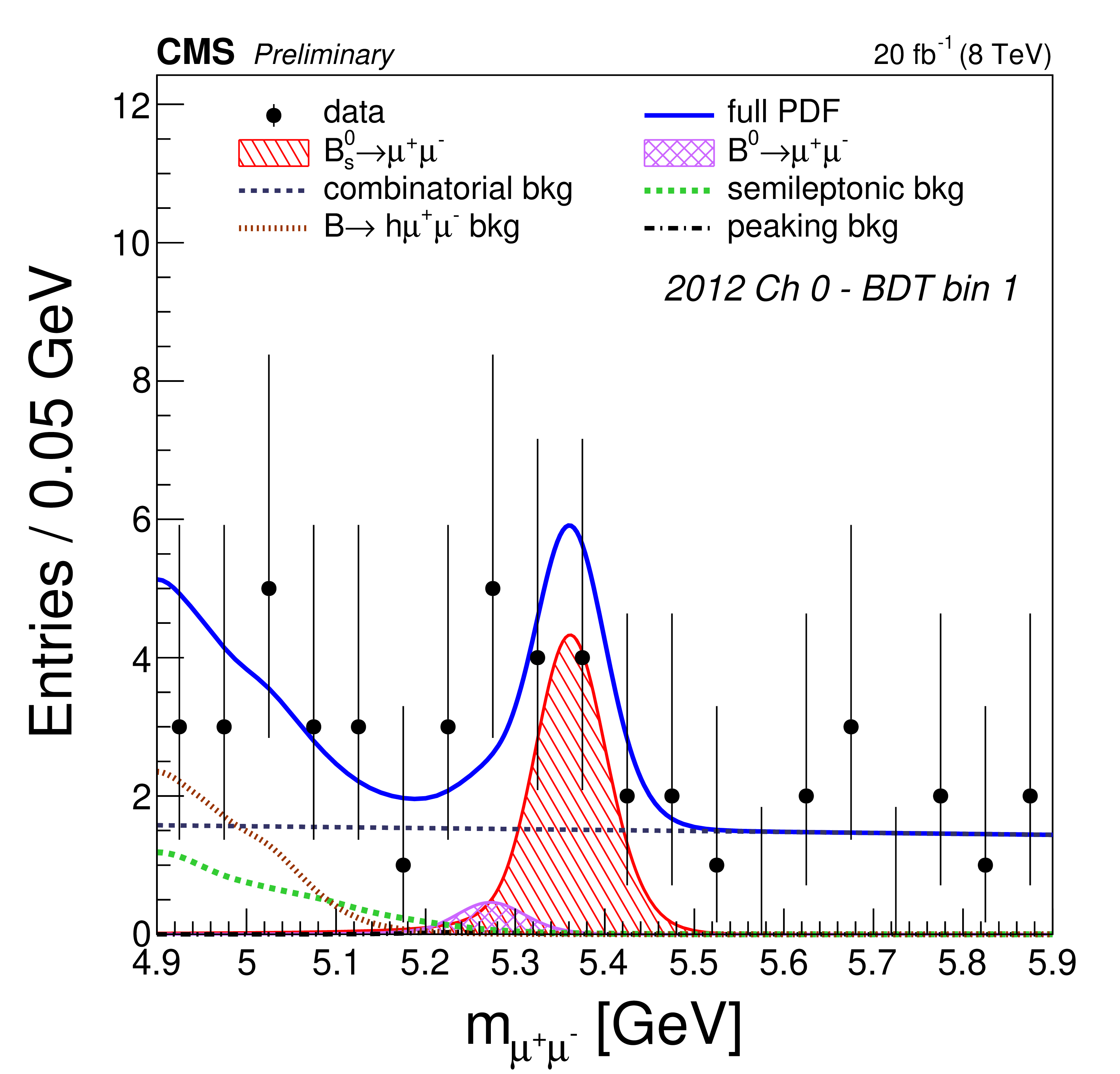
png pdf |
Additional Figure 5-d:
Invariant mass distribution for one of the analysis BDT categories with the fit projection overlays for the branching fraction results. The total fit is shown by the solid line and the different background components by the broken lines. The signal components are shown by the hatched histograms. |
png pdf |
Additional Figure 5-e:
Invariant mass distribution for one of the analysis BDT categories with the fit projection overlays for the branching fraction results. The total fit is shown by the solid line and the different background components by the broken lines. The signal components are shown by the hatched histograms. |
png pdf |
Additional Figure 5-f:
Invariant mass distribution for one of the analysis BDT categories with the fit projection overlays for the branching fraction results. The total fit is shown by the solid line and the different background components by the broken lines. The signal components are shown by the hatched histograms. |
png pdf |
Additional Figure 5-g:
Invariant mass distribution for one of the analysis BDT categories with the fit projection overlays for the branching fraction results. The total fit is shown by the solid line and the different background components by the broken lines. The signal components are shown by the hatched histograms. |
png pdf |
Additional Figure 5-h:
Invariant mass distribution for one of the analysis BDT categories with the fit projection overlays for the branching fraction results. The total fit is shown by the solid line and the different background components by the broken lines. The signal components are shown by the hatched histograms. |
png pdf |
Additional Figure 5-i:
Invariant mass distribution for one of the analysis BDT categories with the fit projection overlays for the branching fraction results. The total fit is shown by the solid line and the different background components by the broken lines. The signal components are shown by the hatched histograms. |
png pdf |
Additional Figure 5-j:
Invariant mass distribution for one of the analysis BDT categories with the fit projection overlays for the branching fraction results. The total fit is shown by the solid line and the different background components by the broken lines. The signal components are shown by the hatched histograms. |
png pdf |
Additional Figure 5-k:
Invariant mass distribution for one of the analysis BDT categories with the fit projection overlays for the branching fraction results. The total fit is shown by the solid line and the different background components by the broken lines. The signal components are shown by the hatched histograms. |
png pdf |
Additional Figure 5-l:
Invariant mass distribution for one of the analysis BDT categories with the fit projection overlays for the branching fraction results. The total fit is shown by the solid line and the different background components by the broken lines. The signal components are shown by the hatched histograms. |
png pdf |
Additional Figure 5-m:
Invariant mass distribution for one of the analysis BDT categories with the fit projection overlays for the branching fraction results. The total fit is shown by the solid line and the different background components by the broken lines. The signal components are shown by the hatched histograms. |
png pdf |
Additional Figure 5-n:
Invariant mass distribution for one of the analysis BDT categories with the fit projection overlays for the branching fraction results. The total fit is shown by the solid line and the different background components by the broken lines. The signal components are shown by the hatched histograms. |
png pdf |
Additional Figure 6:
Invariant mass and proper decay time distributions for each analysis BDT category, with the 2D UML fit projections overlayed. The total fit is shown by the solid line and the different background components by the broken lines and cross-hatched histogram. The signal component is shown by the red single-hatched histogram. |

png pdf |
Additional Figure 6-a:
Invariant mass and proper decay time distributions for one of the analysis BDT categories, with the 2D UML fit projections overlayed. The total fit is shown by the solid line and the different background components by the broken lines and cross-hatched histogram. The signal component is shown by the red single-hatched histogram. |
png pdf |
Additional Figure 6-b:
Invariant mass and proper decay time distributions for one of the analysis BDT categories, with the 2D UML fit projections overlayed. The total fit is shown by the solid line and the different background components by the broken lines and cross-hatched histogram. The signal component is shown by the red single-hatched histogram. |
png pdf |
Additional Figure 6-c:
Invariant mass and proper decay time distributions for one of the analysis BDT categories, with the 2D UML fit projections overlayed. The total fit is shown by the solid line and the different background components by the broken lines and cross-hatched histogram. The signal component is shown by the red single-hatched histogram. |
png pdf |
Additional Figure 6-d:
Invariant mass and proper decay time distributions for one of the analysis BDT categories, with the 2D UML fit projections overlayed. The total fit is shown by the solid line and the different background components by the broken lines and cross-hatched histogram. The signal component is shown by the red single-hatched histogram. |
png pdf |
Additional Figure 6-e:
Invariant mass and proper decay time distributions for one of the analysis BDT categories, with the 2D UML fit projections overlayed. The total fit is shown by the solid line and the different background components by the broken lines and cross-hatched histogram. The signal component is shown by the red single-hatched histogram. |
png pdf |
Additional Figure 6-f:
Invariant mass and proper decay time distributions for one of the analysis BDT categories, with the 2D UML fit projections overlayed. The total fit is shown by the solid line and the different background components by the broken lines and cross-hatched histogram. The signal component is shown by the red single-hatched histogram. |
png pdf |
Additional Figure 6-g:
Invariant mass and proper decay time distributions for one of the analysis BDT categories, with the 2D UML fit projections overlayed. The total fit is shown by the solid line and the different background components by the broken lines and cross-hatched histogram. The signal component is shown by the red single-hatched histogram. |
png pdf |
Additional Figure 6-h:
Invariant mass and proper decay time distributions for one of the analysis BDT categories, with the 2D UML fit projections overlayed. The total fit is shown by the solid line and the different background components by the broken lines and cross-hatched histogram. The signal component is shown by the red single-hatched histogram. |

png pdf |
Additional Figure 6-i:
Invariant mass and proper decay time distributions for one of the analysis BDT categories, with the 2D UML fit projections overlayed. The total fit is shown by the solid line and the different background components by the broken lines and cross-hatched histogram. The signal component is shown by the red single-hatched histogram. |
png pdf |
Additional Figure 6-j:
Invariant mass and proper decay time distributions for one of the analysis BDT categories, with the 2D UML fit projections overlayed. The total fit is shown by the solid line and the different background components by the broken lines and cross-hatched histogram. The signal component is shown by the red single-hatched histogram. |
png pdf |
Additional Figure 6-k:
Invariant mass and proper decay time distributions for one of the analysis BDT categories, with the 2D UML fit projections overlayed. The total fit is shown by the solid line and the different background components by the broken lines and cross-hatched histogram. The signal component is shown by the red single-hatched histogram. |
png pdf |
Additional Figure 6-l:
Invariant mass and proper decay time distributions for one of the analysis BDT categories, with the 2D UML fit projections overlayed. The total fit is shown by the solid line and the different background components by the broken lines and cross-hatched histogram. The signal component is shown by the red single-hatched histogram. |
png pdf |
Additional Figure 6-m:
Invariant mass and proper decay time distributions for one of the analysis BDT categories, with the 2D UML fit projections overlayed. The total fit is shown by the solid line and the different background components by the broken lines and cross-hatched histogram. The signal component is shown by the red single-hatched histogram. |
png pdf |
Additional Figure 6-n:
Invariant mass and proper decay time distributions for one of the analysis BDT categories, with the 2D UML fit projections overlayed. The total fit is shown by the solid line and the different background components by the broken lines and cross-hatched histogram. The signal component is shown by the red single-hatched histogram. |
png pdf |
Additional Figure 6-o:
Invariant mass and proper decay time distributions for one of the analysis BDT categories, with the 2D UML fit projections overlayed. The total fit is shown by the solid line and the different background components by the broken lines and cross-hatched histogram. The signal component is shown by the red single-hatched histogram. |
png pdf |
Additional Figure 6-p:
Invariant mass and proper decay time distributions for one of the analysis BDT categories, with the 2D UML fit projections overlayed. The total fit is shown by the solid line and the different background components by the broken lines and cross-hatched histogram. The signal component is shown by the red single-hatched histogram. |
png pdf |
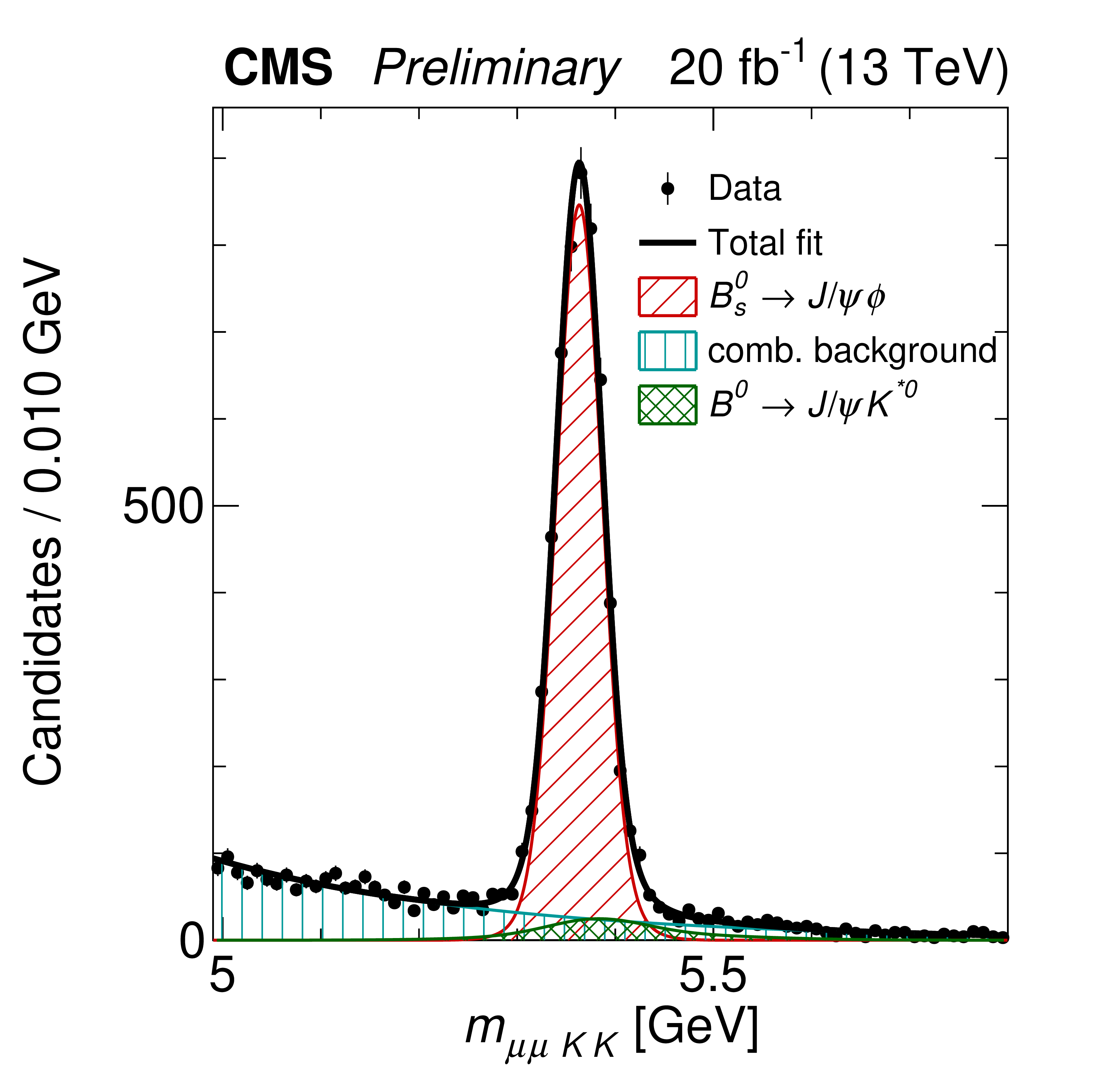
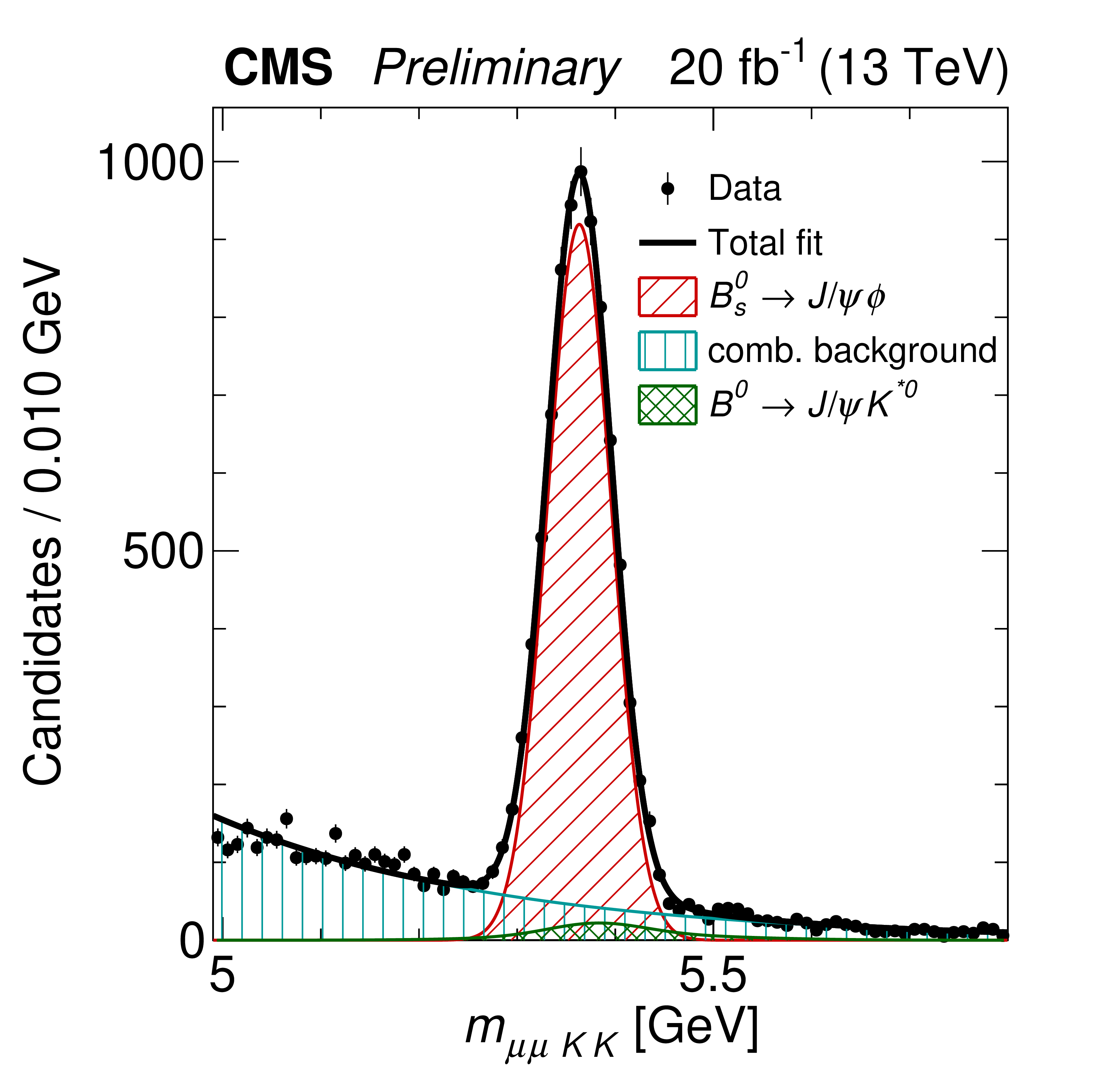
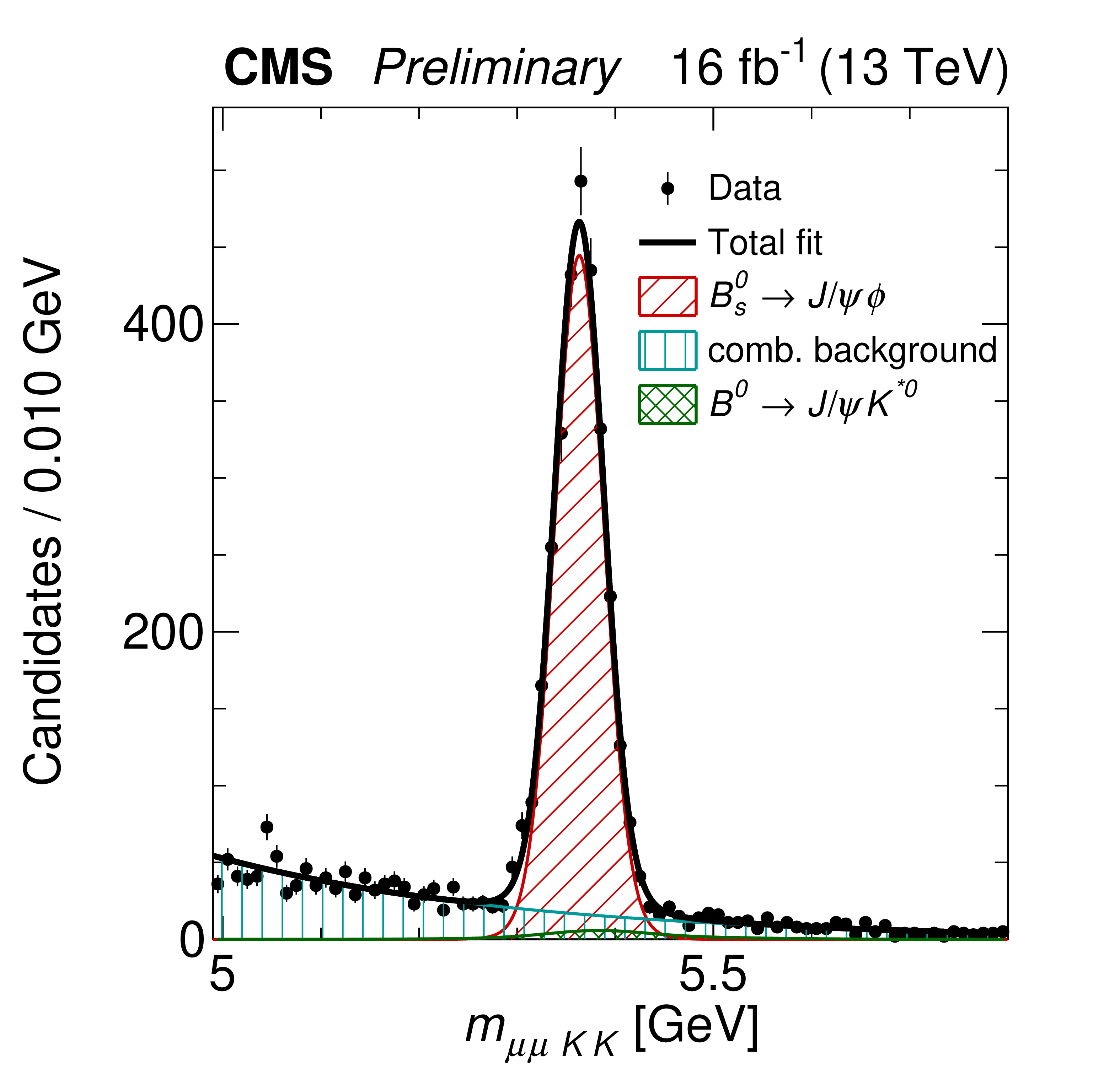
Additional Figure 7:
Invariant-mass distributions for the $\mu \mu \mathrm{K}$ (top) and $\mu \mu \mathrm{KK}$ (bottom) systems used to reconstruct the $\mathrm{B}^{+}\to \mathrm{J}/\psi \mathrm{K}^+$ normalization samples. From left to right, the plot shows the 2016A central-region, 2016A forward-region, 2016B central-region, and 2016B forward-region channels. The data are shown by solid black circles, the result of the fit is overlayed with the black line, and the different components are indicated by the hatched regions. |
png pdf |
Additional Figure 7-a:
Invariant-mass distribution for the $\mu \mu \mathrm{K}$ system used to reconstruct the $\mathrm{B}^{+}\to \mathrm{J}/\psi \mathrm{K}^+$ normalization sample. The plot shows the 2016A central-region channel. The data are shown by solid black circles, the result of the fit is overlayed with the black line, and the different components are indicated by the hatched regions. |
png pdf |
Additional Figure 7-b:
Invariant-mass distribution for the $\mu \mu \mathrm{K}$ system used to reconstruct the $\mathrm{B}^{+}\to \mathrm{J}/\psi \mathrm{K}^+$ normalization sample. The plot shows the 2016A forward-region channel. The data are shown by solid black circles, the result of the fit is overlayed with the black line, and the different components are indicated by the hatched regions. |

png pdf |
Additional Figure 7-c:
Invariant-mass distribution for the $\mu \mu \mathrm{K}$ system used to reconstruct the $\mathrm{B}^{+}\to \mathrm{J}/\psi \mathrm{K}^+$ normalization sample. The plot shows the 2016B central-region channel. The data are shown by solid black circles, the result of the fit is overlayed with the black line, and the different components are indicated by the hatched regions. |
png pdf |
Additional Figure 7-d:
Invariant-mass distribution for the $\mu \mu \mathrm{K}$ system used to reconstruct the $\mathrm{B}^{+}\to \mathrm{J}/\psi \mathrm{K}^+$ normalization sample. The plot shows the 2016B forward-region channel. The data are shown by solid black circles, the result of the fit is overlayed with the black line, and the different components are indicated by the hatched regions. |
png pdf |
Additional Figure 7-e:
Invariant-mass distributions for the $\mu \mu \mathrm{K}$ (top) and $\mu \mu \mathrm{KK}$ (bottom) systems used to reconstruct the $\mathrm{B}^{+}\to \mathrm{J}/\psi \mathrm{K}^+$ normalization samples. From left to right, the plot shows the 2016A central-region, 2016A forward-region, 2016B central-region, and 2016B forward-region channels. The data are shown by solid black circles, the result of the fit is overlayed with the black line, and the different components are indicated by the hatched regions. |
png pdf |
Additional Figure 7-f:
Invariant-mass distribution for the $\mu \mu \mathrm{KK}$ system used to reconstruct the $\mathrm{B_s}^{0}\to \mathrm{J}/\psi \phi $ control sample. The plot shows the 2016A forward-region channel. The data are shown by solid black circles, the result of the fit is overlayed with the black line, and the different components are indicated by the hatched regions. |
png pdf |
Additional Figure 7-g:
Invariant-mass distribution for the $\mu \mu \mathrm{KK}$ system used to reconstruct the $\mathrm{B_s}^{0}\to \mathrm{J}/\psi \phi $ control sample. The plot shows the2016B central-region channel. The data are shown by solid black circles, the result of the fit is overlayed with the black line, and the different components are indicated by the hatched regions. |
png pdf |
Additional Figure 7-h:
Invariant-mass distribution for the $\mu \mu \mathrm{KK}$ system used to reconstruct the $\mathrm{B_s}^{0}\to \mathrm{J}/\psi \phi $ control sample. The plot shows the 2016B forward-region channel. The data are shown by solid black circles, the result of the fit is overlayed with the black line, and the different components are indicated by the hatched regions. |
png pdf |
Additional Figure 8:
Expected mass distributions from MC simulations for a combination of all rare processes (left), of all rare semileptonic decays (middle), and of rare two-body hadronic background components (right), corresponding to the sum of all categories of the high-BDT mass plot. |

png pdf |
Additional Figure 8-a:
Expected mass distribution from MC simulations for a combination of all rare processes, corresponding to the sum of all categories of the high-BDT mass plot. |
png pdf |
Additional Figure 8-b:
Expected mass distribution from MC simulations for a combination of all rare semileptonic decays, corresponding to the sum of all categories of the high-BDT mass plot. |
png pdf |
Additional Figure 8-c:
Expected mass distribution from MC simulations for a combination of rare two-body hadronic background components, corresponding to the sum of all categories of the high-BDT mass plot. |
png pdf |
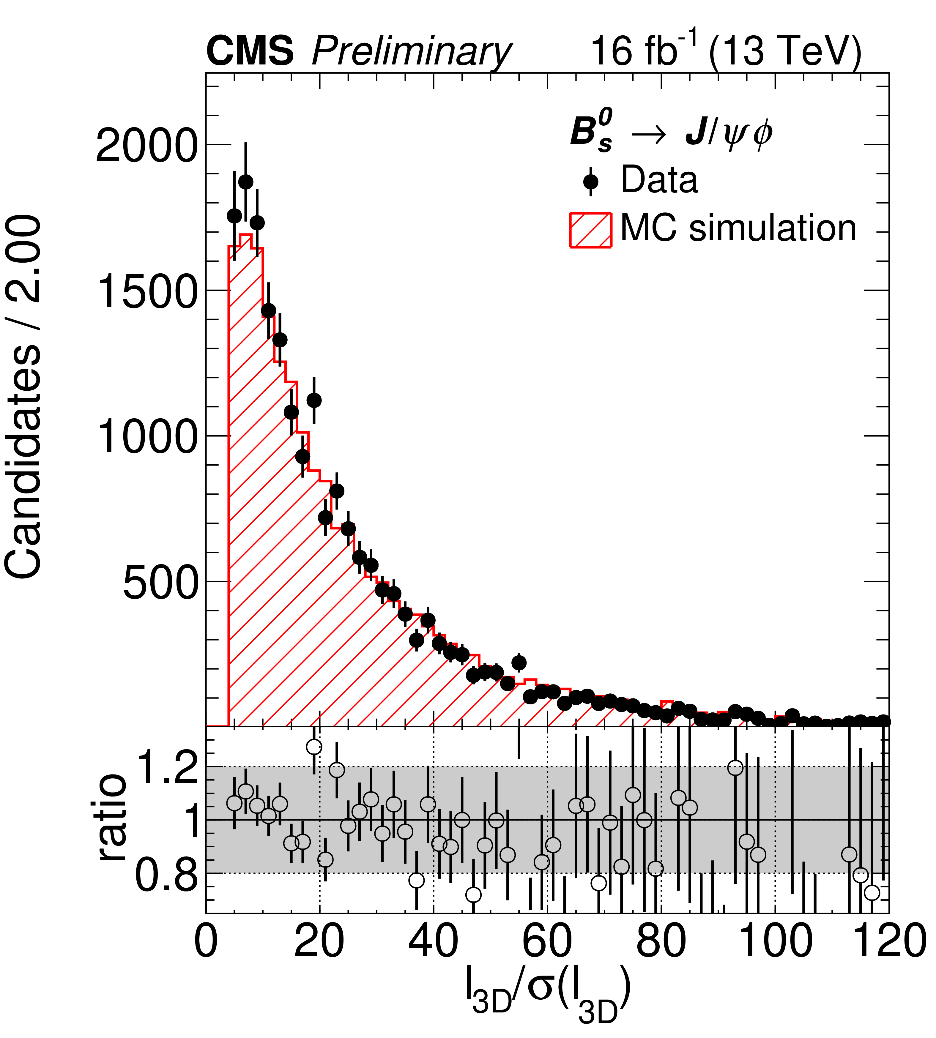
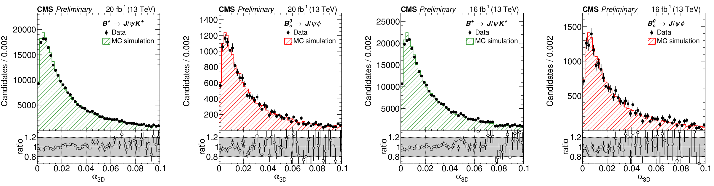
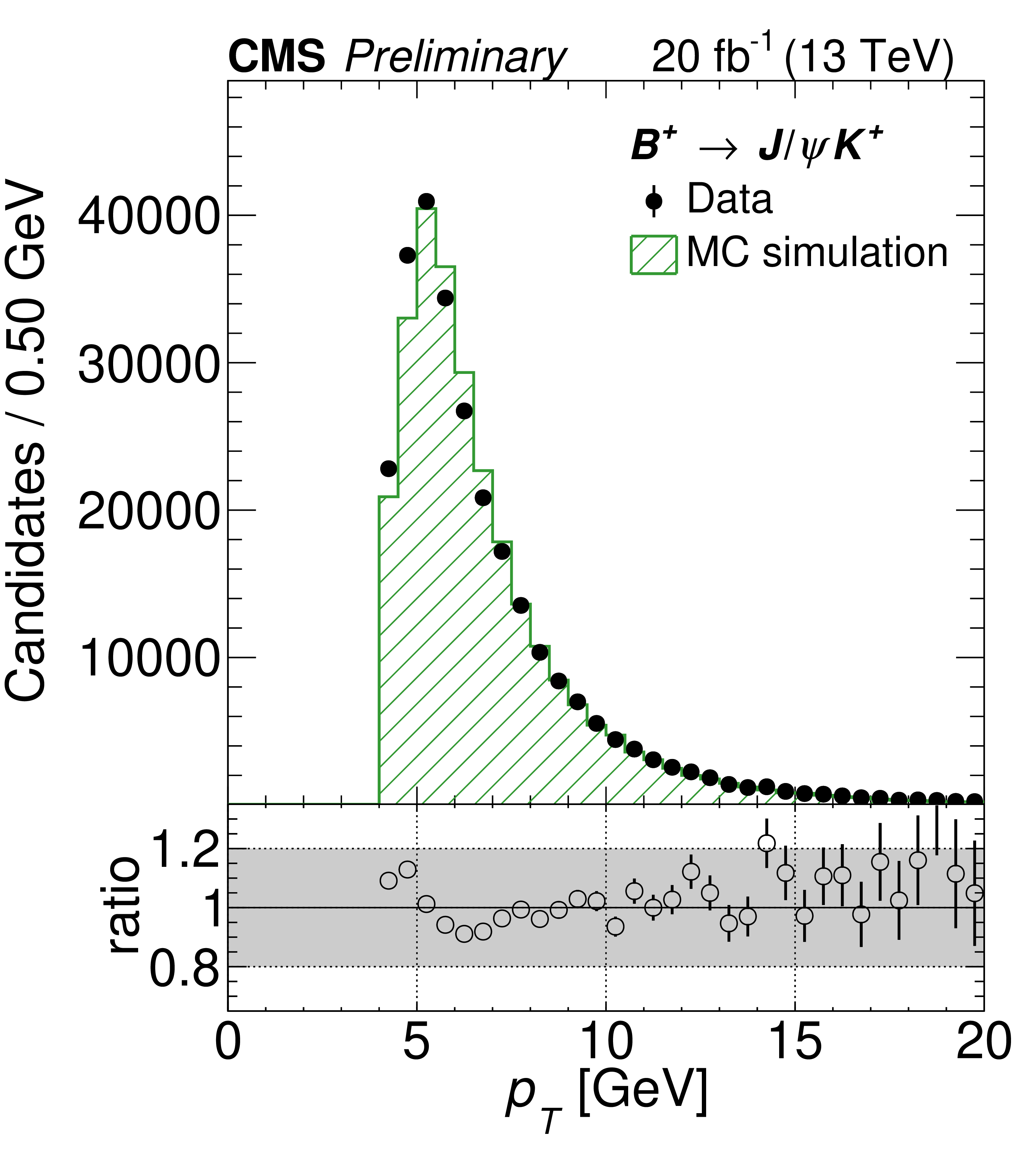
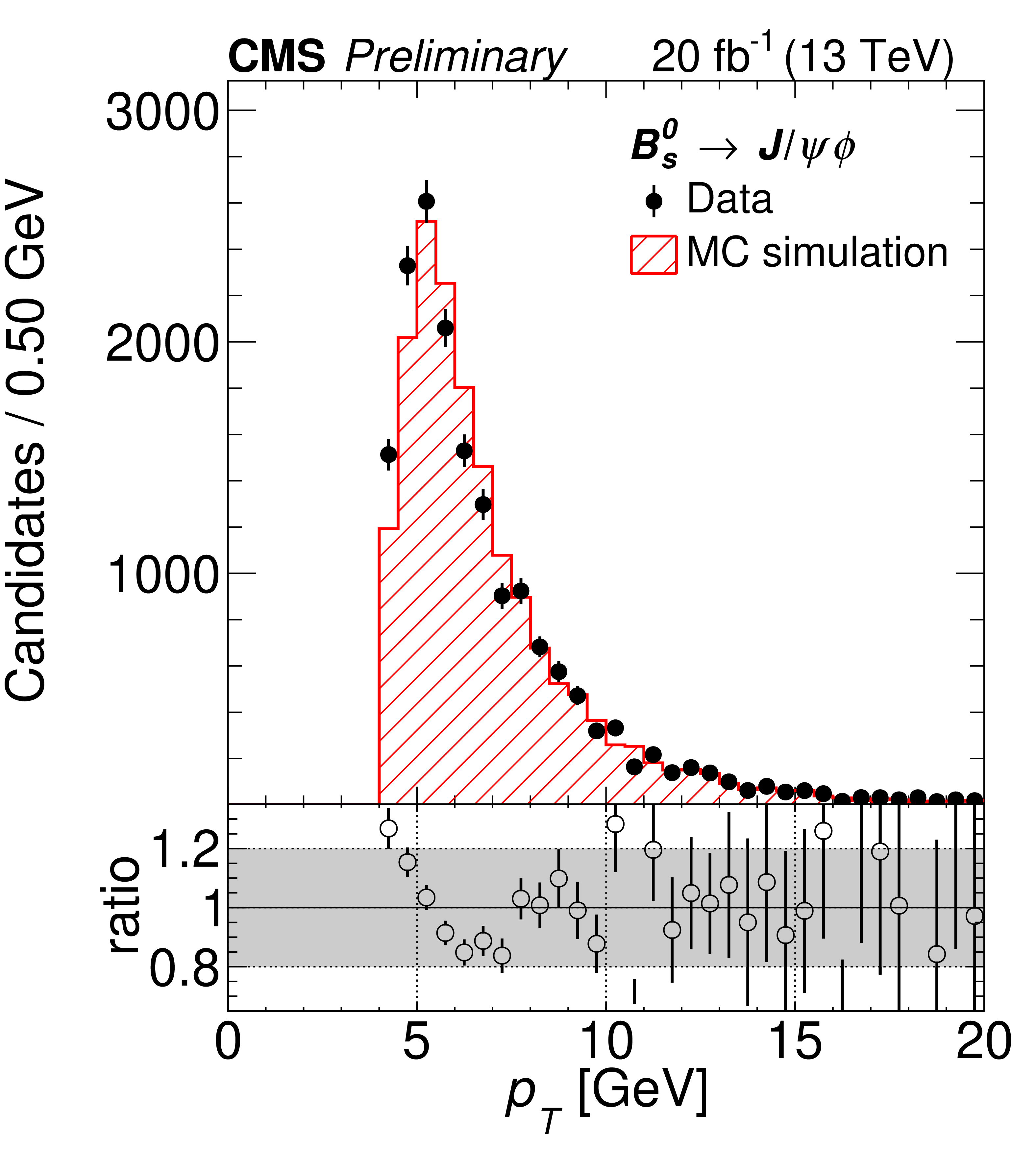
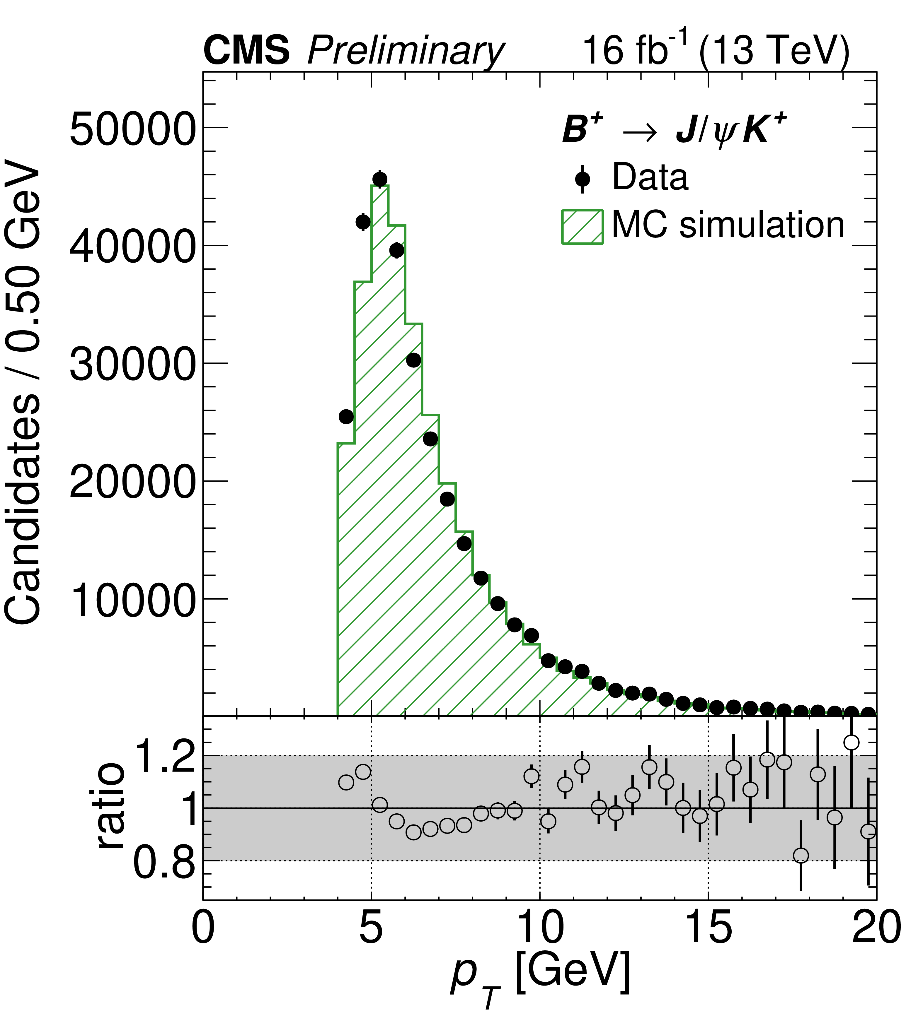
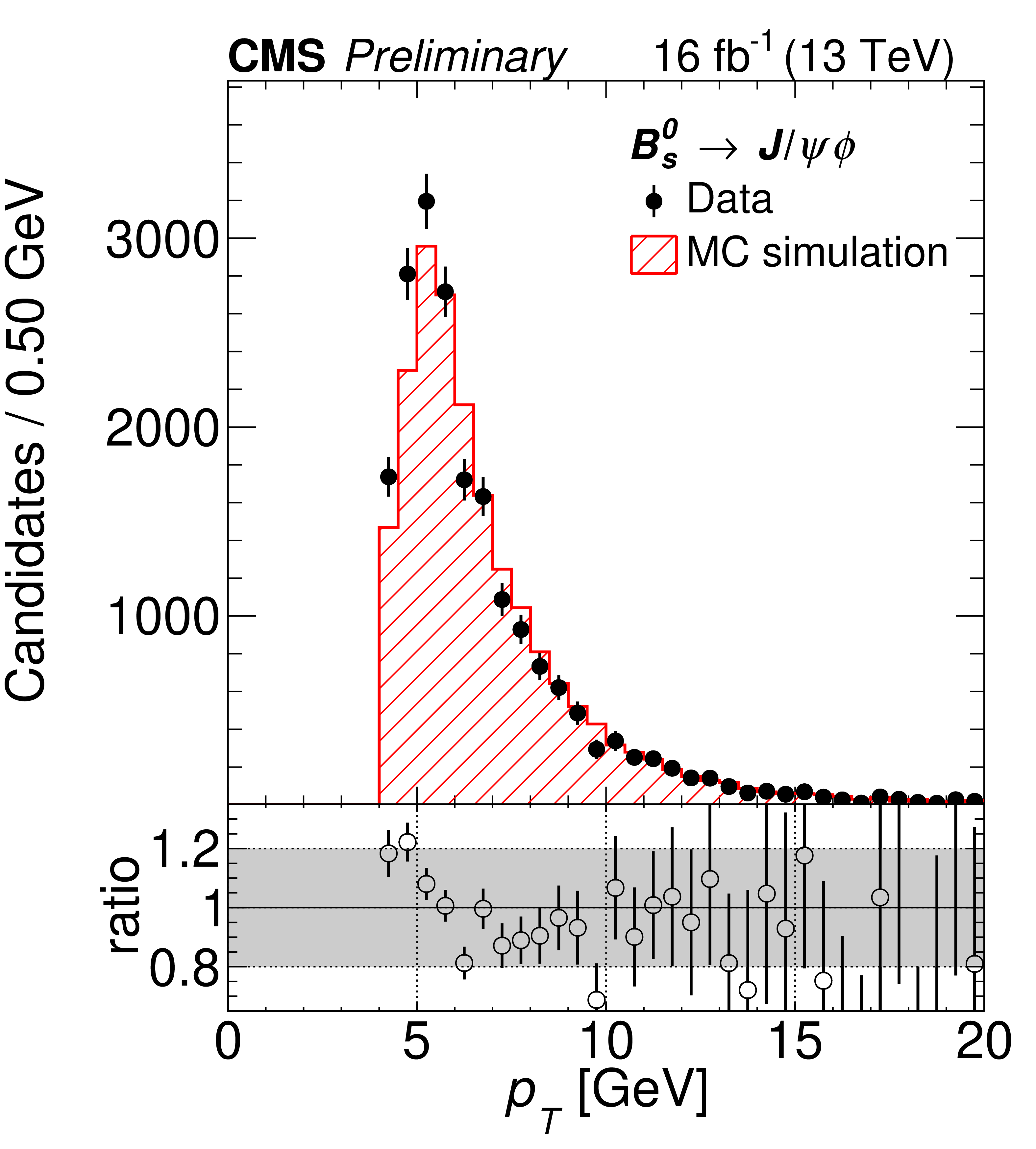
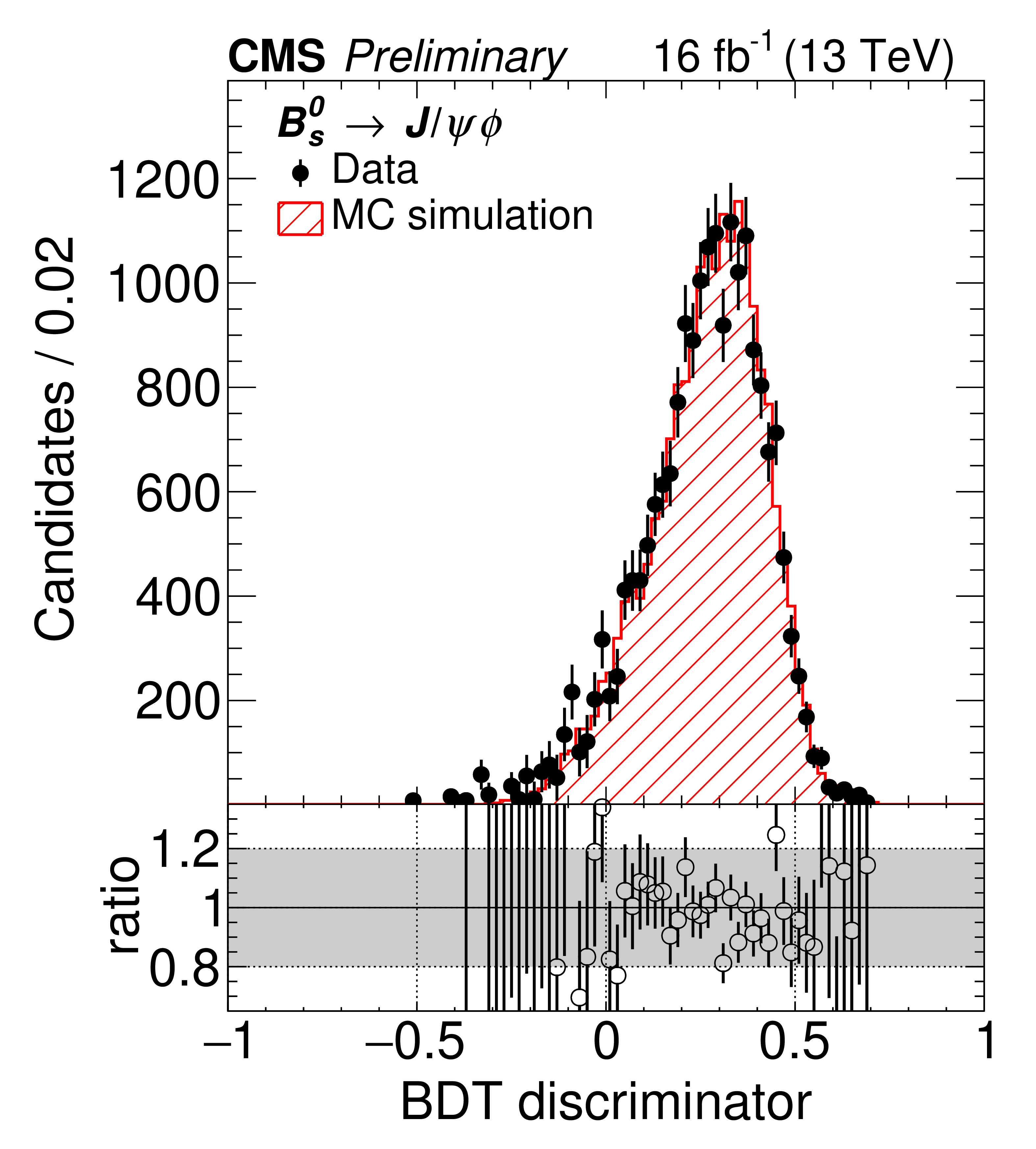
Additional Figure 9:
Comparison of measured and simulated distributions for the flight length significance in central-region channel. From left to right, the plot shows the distribution for 2016A $\mathrm{B}^{+}\to \mathrm{J}/\psi \mathrm{K}^+$, 2016A $\mathrm{B_s}^{0}\to \mathrm{J}/\psi \phi $, 2016B $\mathrm{B}^{+}\to \mathrm{J}/\psi \mathrm{K}^+$, and 2016B $\mathrm{B_s}^{0}\to \mathrm{J}/\psi \phi $ candidates. |
png pdf |
Additional Figure 9-a:
Comparison of measured and simulated distributions for the flight length significance in central-region channel. From left to right, the plot shows the distribution for 2016A $\mathrm{B}^{+}\to \mathrm{J}/\psi \mathrm{K}^+$ candidates. |
png pdf |
Additional Figure 9-b:
Comparison of measured and simulated distributions for the flight length significance in central-region channel. From left to right, the plot shows the distribution for 2016A $\mathrm{B_s}^{0}\to \mathrm{J}/\psi \phi $ candidates. |
png pdf |
Additional Figure 9-c:
Comparison of measured and simulated distributions for the flight length significance in central-region channel. From left to right, the plot shows the distribution for 2016B $\mathrm{B}^{+}\to \mathrm{J}/\psi \mathrm{K}^+$ candidates. |
png pdf |
Additional Figure 9-d:
Comparison of measured and simulated distributions for the flight length significance in central-region channel. From left to right, the plot shows the distribution for 2016B $\mathrm{B_s}^{0}\to \mathrm{J}/\psi \phi $ candidates. |
png pdf |
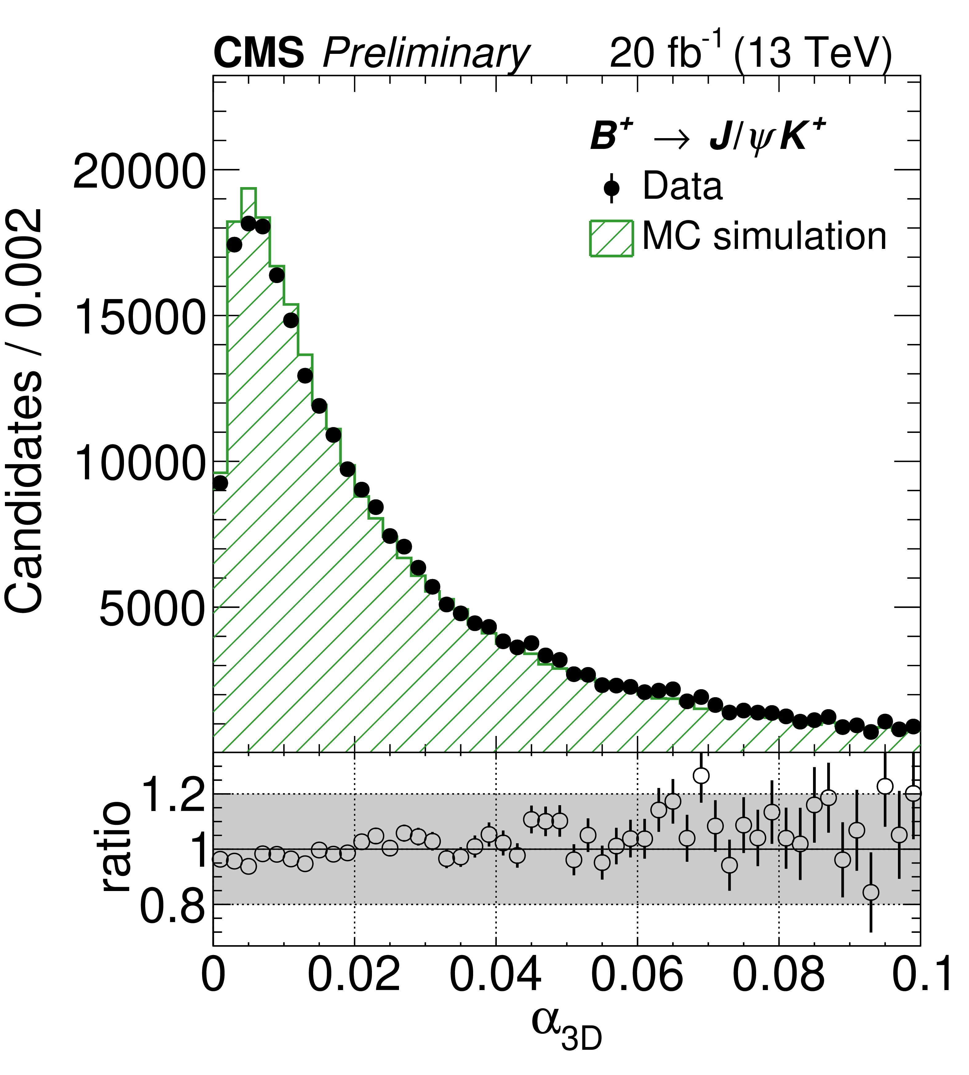
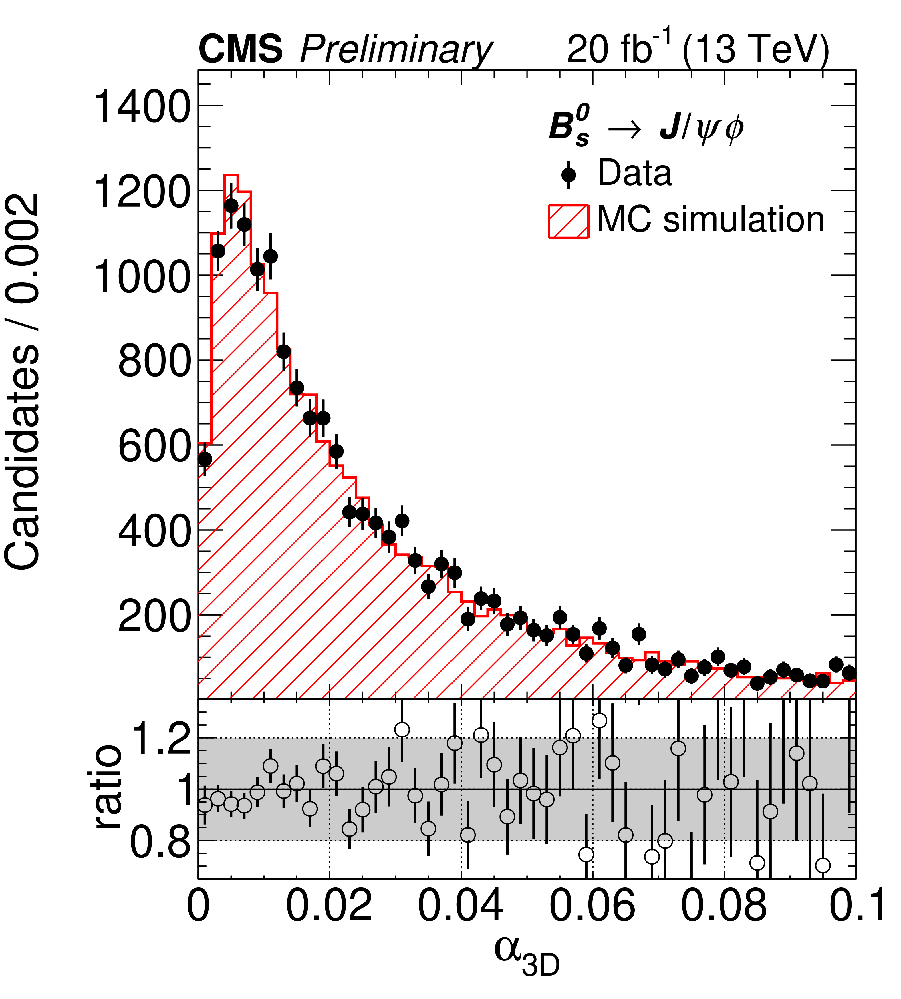
Additional Figure 10:
Comparison of measured and simulated distributions for the pointing angle (defined in the main text) in central-region channel. From left to right, the plot shows the distribution for 2016A $\mathrm{B}^{+}\to \mathrm{J}/\psi \mathrm{K}^+$, 2016A $\mathrm{B_s}^{0}\to \mathrm{J}/\psi \phi $, 2016B $\mathrm{B}^{+}\to \mathrm{J}/\psi \mathrm{K}^+$, and 2016B $\mathrm{B_s}^{0}\to \mathrm{J}/\psi \phi $ candidates. |
png pdf |
Additional Figure 10-a:
Comparison of measured and simulated distributions for the pointing angle (defined in the main text) in central-region channel. The plot shows the distribution for 2016A $\mathrm{B}^{+}\to \mathrm{J}/\psi \mathrm{K}^+$ candidates. |
png pdf |
Additional Figure 10-b:
Comparison of measured and simulated distributions for the pointing angle (defined in the main text) in central-region channel. The plot shows the distribution for 2016A $\mathrm{B_s}^{0}\to \mathrm{J}/\psi \phi $ candidates. |
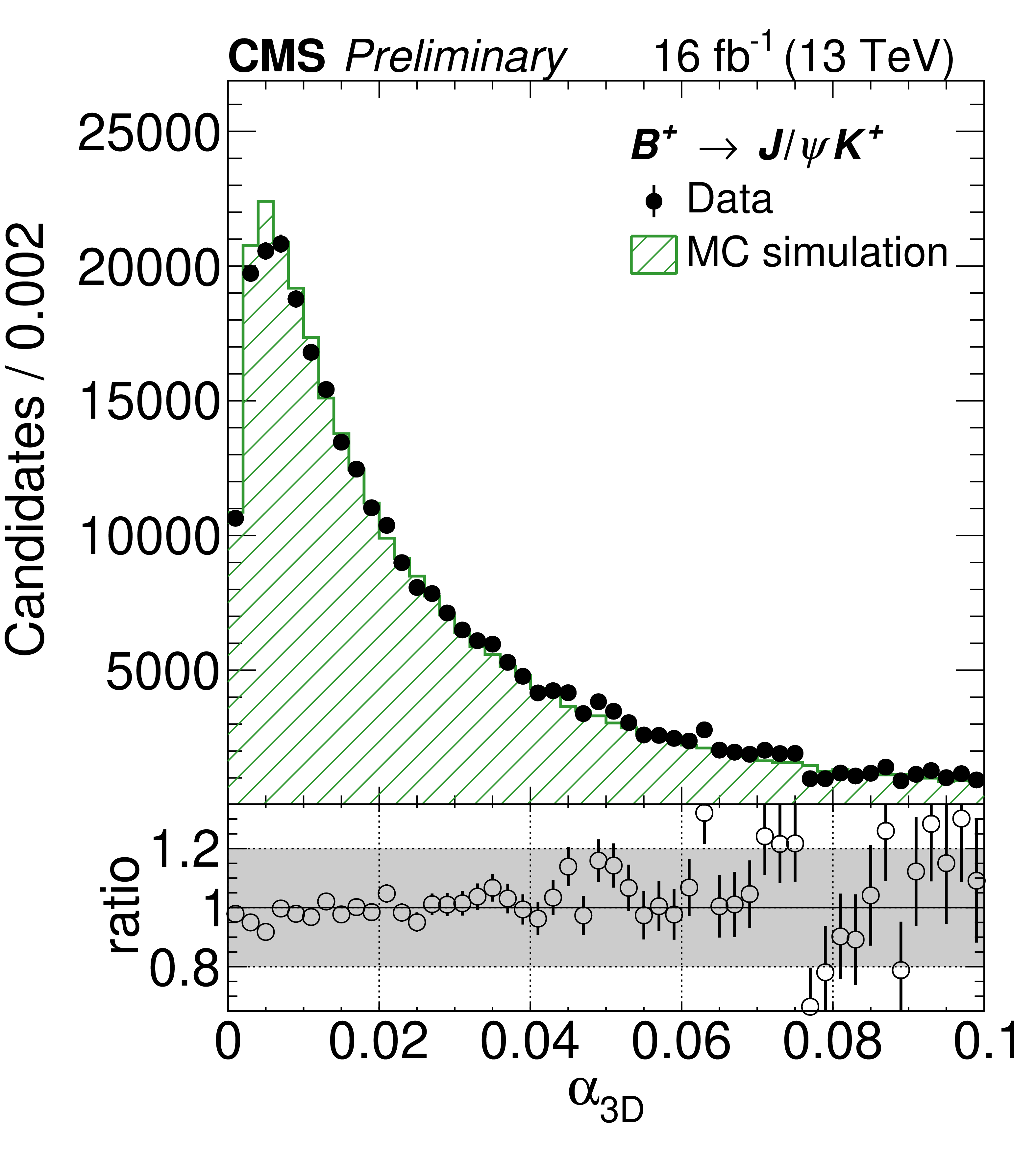
png pdf |
Additional Figure 10-c:
Comparison of measured and simulated distributions for the pointing angle (defined in the main text) in central-region channel. The plot shows the distribution for 2016B $\mathrm{B}^{+}\to \mathrm{J}/\psi \mathrm{K}^+$ candidates. |
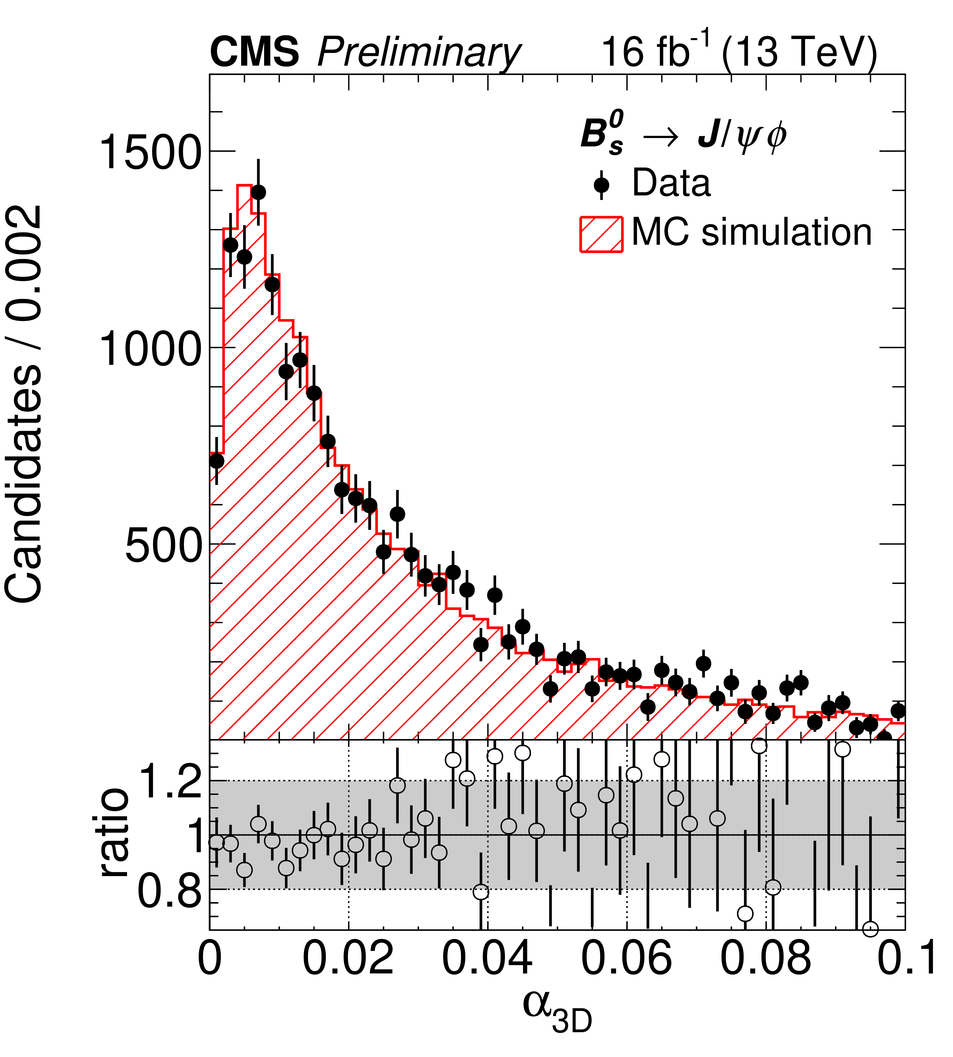
png pdf |
Additional Figure 10-d:
Comparison of measured and simulated distributions for the pointing angle (defined in the main text) in central-region channel. The plot shows the distribution for 2016B $\mathrm{B_s}^{0}\to \mathrm{J}/\psi \phi $ candidates. |
png pdf |
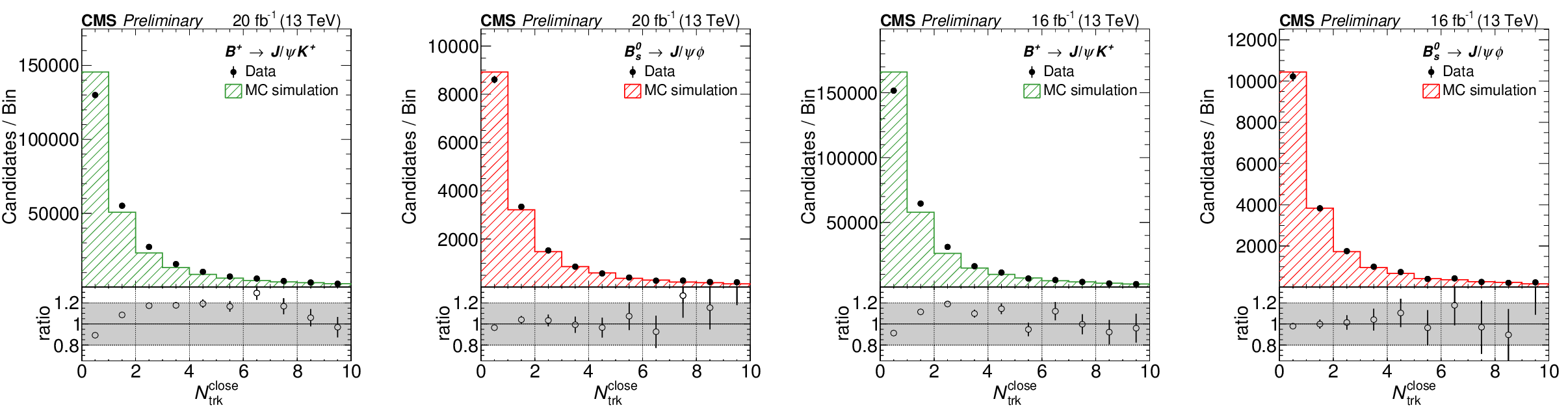
Additional Figure 11:
Comparison of measured and simulated distributions for the number of tracks close to the secondary vertex in central-region channel. From left to right, the plot shows the distribution for 2016A $\mathrm{B}^{+}\to \mathrm{J}/\psi \mathrm{K}^+$, 2016A $\mathrm{B_s}^{0}\to \mathrm{J}/\psi \phi $, 2016B $\mathrm{B}^{+}\to \mathrm{J}/\psi \mathrm{K}^+$, and 2016B $\mathrm{B_s}^{0}\to \mathrm{J}/\psi \phi $ candidates. |
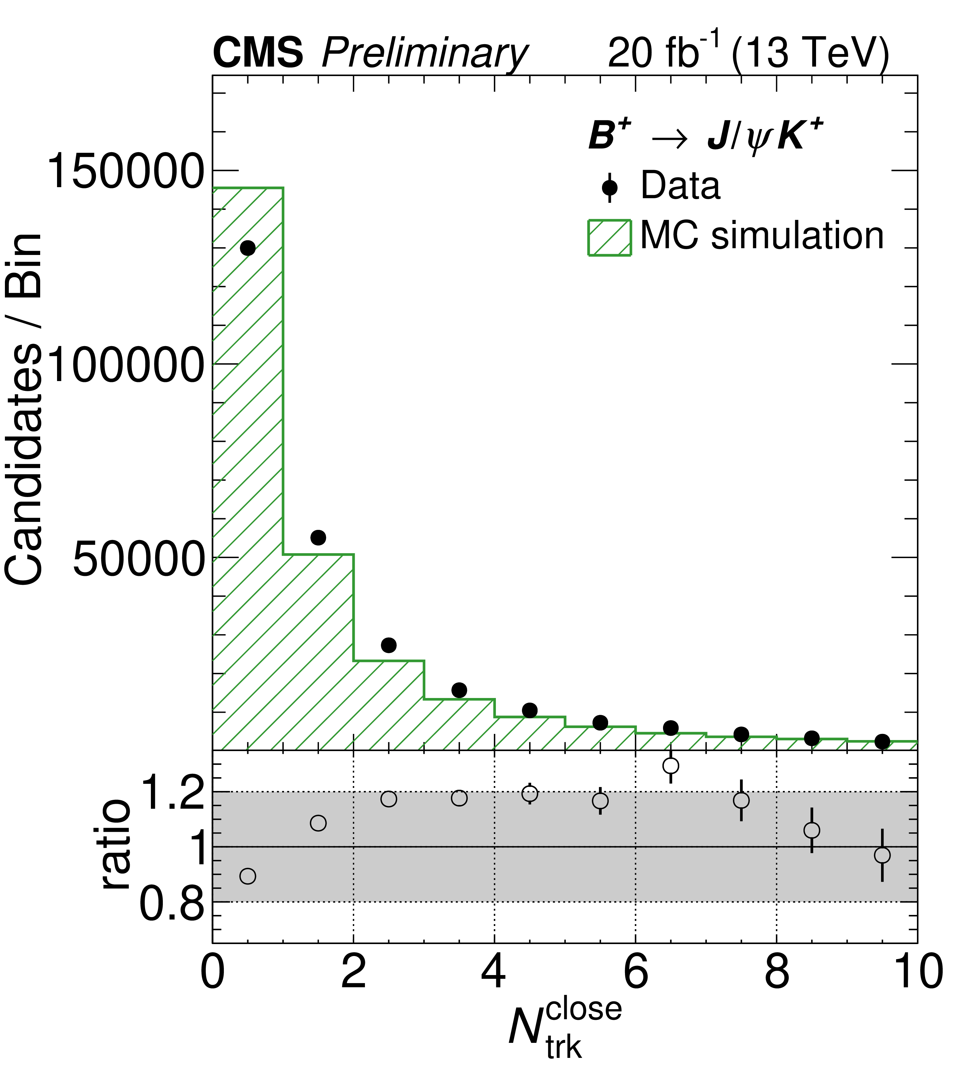
png pdf |
Additional Figure 11-a:
Comparison of measured and simulated distributions for the number of tracks close to the secondary vertex in central-region channel. The plot shows the distribution for 2016A $\mathrm{B}^{+}\to \mathrm{J}/\psi \mathrm{K}^+$ candidates. |
png pdf |
Additional Figure 11-b:
Comparison of measured and simulated distributions for the number of tracks close to the secondary vertex in central-region channel. The plot shows the distribution for 2016A $\mathrm{B_s}^{0}\to \mathrm{J}/\psi \phi $ candidates. |
png pdf |
Additional Figure 11-c:
Comparison of measured and simulated distributions for the number of tracks close to the secondary vertex in central-region channel. The plot shows the distribution for 2016B $\mathrm{B}^{+}\to \mathrm{J}/\psi \mathrm{K}^+$ candidates. |
png pdf |
Additional Figure 11-d:
Comparison of measured and simulated distributions for the number of tracks close to the secondary vertex in central-region channel. The plot shows the distribution for 2016B $\mathrm{B_s}^{0}\to \mathrm{J}/\psi \phi $ candidates. |
png pdf |
Additional Figure 12:
Comparison of measured and simulated distributions for the subleading muon $p_{\rm T}$ in central-region channel. From left to right, the plot shows the distribution for 2016A $\mathrm{B}^{+}\to \mathrm{J}/\psi \mathrm{K}^+$, 2016A $\mathrm{B_s}^{0}\to \mathrm{J}/\psi \phi $, 2016B $\mathrm{B}^{+}\to \mathrm{J}/\psi \mathrm{K}^+$, and 2016B $\mathrm{B_s}^{0}\to \mathrm{J}/\psi \phi $ candidates. |
png pdf |
Additional Figure 12-a:
Comparison of measured and simulated distributions for the subleading muon $p_{\rm T}$ in central-region channel. The plot shows the distribution for 2016A $\mathrm{B}^{+}\to \mathrm{J}/\psi \mathrm{K}^+$ candidates. |
png pdf |
Additional Figure 12-b:
Comparison of measured and simulated distributions for the subleading muon $p_{\rm T}$ in central-region channel. The plot shows the distribution for 2016A $\mathrm{B_s}^{0}\to \mathrm{J}/\psi \phi $ candidates. |
png pdf |
Additional Figure 12-c:
Comparison of measured and simulated distributions for the subleading muon $p_{\rm T}$ in central-region channel. The plot shows the distribution for 2016B $\mathrm{B}^{+}\to \mathrm{J}/\psi \mathrm{K}^+$ candidates. |
png pdf |
Additional Figure 12-d:
Comparison of measured and simulated distributions for the subleading muon $p_{\rm T}$ in central-region channel. The plot shows the distribution for 2016B $\mathrm{B_s}^{0}\to \mathrm{J}/\psi \phi $ candidates. |
png pdf |
Additional Figure 13:
Comparison of measured and simulated distributions for the muon helicity angle for 2016A (left) and 2016B (right) $\mathrm{B}^{+}\to \mathrm{J}/\psi \mathrm{K}^+$ candidates in central-region channel. |
png pdf |
Additional Figure 13-a:
Comparison of measured and simulated distributions for the muon helicity angle for 2016A $\mathrm{B}^{+}\to \mathrm{J}/\psi \mathrm{K}^+$ candidates in central-region channel. |
png pdf |
Additional Figure 13-b:
Comparison of measured and simulated distributions for the muon helicity angle for 2016B $\mathrm{B}^{+}\to \mathrm{J}/\psi \mathrm{K}^+$ candidates in central-region channel. |

png pdf |
Additional Figure 14:
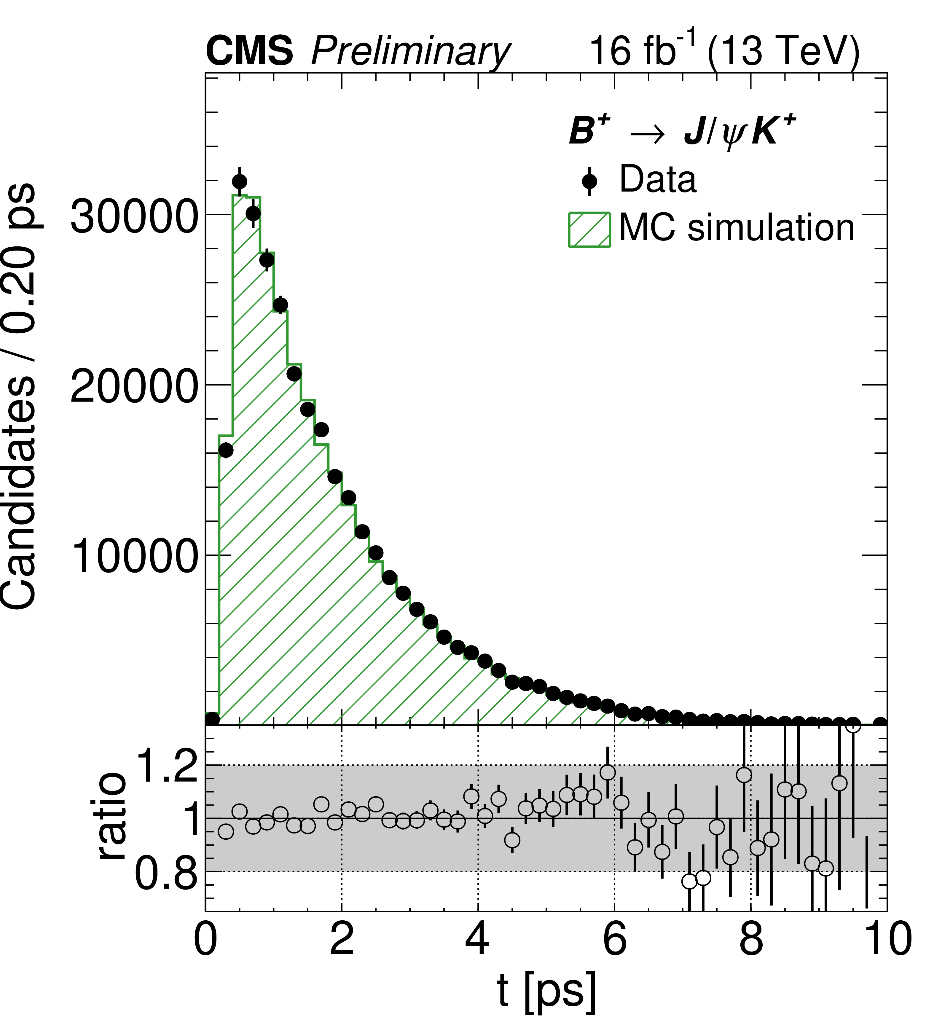
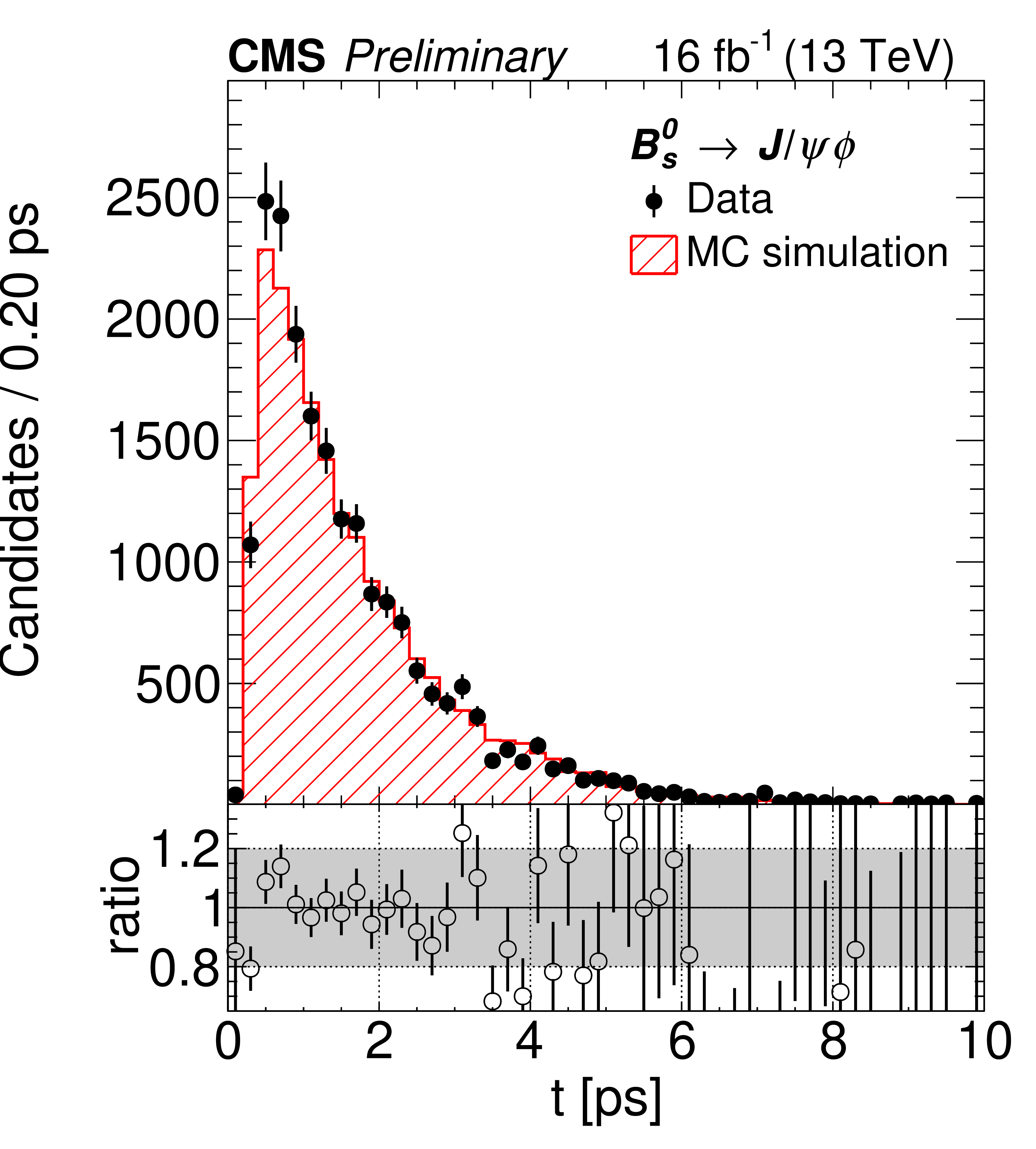
Comparison of measured and simulated distributions for the $B$ meson proper decay time in central-region channel. From left to right, the plot shows the distribution for 2016A $\mathrm{B}^{+}\to \mathrm{J}/\psi \mathrm{K}^+$, 2016A $\mathrm{B_s}^{0}\to \mathrm{J}/\psi \phi $, 2016B $\mathrm{B}^{+}\to \mathrm{J}/\psi \mathrm{K}^+$, and 2016B $\mathrm{B_s}^{0}\to \mathrm{J}/\psi \phi $ candidates. |
png pdf |
Additional Figure 14-a:
Comparison of measured and simulated distributions for the $B$ meson proper decay time in central-region channel. The plot shows the distribution for 2016B $\mathrm{B_s}^{0}\to \mathrm{J}/\psi \phi $ candidates. |
png pdf |
Additional Figure 14-b:
Comparison of measured and simulated distributions for the $B$ meson proper decay time in central-region channel. The plot shows the distribution for 2016A $\mathrm{B_s}^{0}\to \mathrm{J}/\psi \phi $ candidates. |
png pdf |
Additional Figure 14-c:
Comparison of measured and simulated distributions for the $B$ meson proper decay time in central-region channel. The plot shows the distribution for 2016B $\mathrm{B}^{+}\to \mathrm{J}/\psi \mathrm{K}^+$ candidates. |
png pdf |
Additional Figure 14-d:
Comparison of measured and simulated distributions for the $B$ meson proper decay time in central-region channel. From left to right, the plot shows the distribution for 2016A $\mathrm{B}^{+}\to \mathrm{J}/\psi \mathrm{K}^+$, 2016A $\mathrm{B_s}^{0}\to \mathrm{J}/\psi \phi $, 2016B $\mathrm{B}^{+}\to \mathrm{J}/\psi \mathrm{K}^+$, and 2016B $\mathrm{B_s}^{0}\to \mathrm{J}/\psi \phi $ candidates. |
png pdf |
Additional Figure 15:
Illustration of the analysis BDT discriminator distributions in background-subtracted data and MC simulation in the central channel. In top row, from left to right, the plot shows the distribution for 2011 $\mathrm{B}^{+}\to \mathrm{J}/\psi \mathrm{K}^+$, 2011 $\mathrm{B_s}^{0}\to \mathrm{J}/\psi \phi $, 2012 $\mathrm{B}^{+}\to \mathrm{J}/\psi \mathrm{K}^+$, and 2012 $\mathrm{B_s}^{0}\to \mathrm{J}/\psi \phi $ candidates. In the bottom row, the plots (from left to right) show the distribution for 2016A $\mathrm{B}^{+}\to \mathrm{J}/\psi \mathrm{K}^+$, 2016A $\mathrm{B_s}^{0}\to \mathrm{J}/\psi \phi $, 2016B $\mathrm{B}^{+}\to \mathrm{J}/\psi \mathrm{K}^+$, and 2016B $\mathrm{B_s}^{0}\to \mathrm{J}/\psi \phi $ candidates. |
png pdf |
Additional Figure 15-a:
Illustration of the analysis BDT discriminator distributions in background-subtracted data and MC simulation in the central channel. The plot shows the distribution for 2011 $\mathrm{B}^{+}\to \mathrm{J}/\psi \mathrm{K}^+$ candidates. |

png pdf |
Additional Figure 15-b:
Illustration of the analysis BDT discriminator distributions in background-subtracted data and MC simulation in the central channel. The plot shows the distribution for 2011 $\mathrm{B_s}^{0}\to \mathrm{J}/\psi \phi $ candidates. |
png pdf |
Additional Figure 15-c:
Illustration of the analysis BDT discriminator distributions in background-subtracted data and MC simulation in the central channel. The plot shows the distribution for 2012 $\mathrm{B}^{+}\to \mathrm{J}/\psi \mathrm{K}^+$ candidates. |
png pdf |
Additional Figure 15-d:
Illustration of the analysis BDT discriminator distributions in background-subtracted data and MC simulation in the central channel. The plot shows the distribution for 2012 $\mathrm{B_s}^{0}\to \mathrm{J}/\psi \phi $ candidates. |
png pdf |
Additional Figure 15-e:
Illustration of the analysis BDT discriminator distributions in background-subtracted data and MC simulation in the central channel. The plot shows the distribution for 2016A $\mathrm{B}^{+}\to \mathrm{J}/\psi \mathrm{K}^+$ candidates. |

png pdf |
Additional Figure 15-f:
Illustration of the analysis BDT discriminator distributions in background-subtracted data and MC simulation in the central channel. The plot shows the distribution for 2016A $\mathrm{B_s}^{0}\to \mathrm{J}/\psi \phi $ candidates. |
png pdf |
Additional Figure 15-g:
Illustration of the analysis BDT discriminator distributions in background-subtracted data and MC simulation in the central channel. The plot shows the distribution for 2016B $\mathrm{B}^{+}\to \mathrm{J}/\psi \mathrm{K}^+$ candidates. |
png pdf |
Additional Figure 15-h:
Illustration of the analysis BDT discriminator distributions in background-subtracted data and MC simulation in the central channel. The plot shows the distribution for 2016B $\mathrm{B_s}^{0}\to \mathrm{J}/\psi \phi $ candidates. |
png pdf |
Additional Figure 16:
Illustration of the analysis BDT discriminator distribution in dimuon background data from the 5.45 $ < m_{\mu ^+\mu ^-} < $ 5.9 GeV sideband and $\mathrm{B_s}^{0}\to \mu ^+\mu ^-$ signal MC simulation. In top row, from left to right the plot shows the distribution for 2011 central, 2011 forward, 2012 central, and 2012 forward events. In the bottom row, the plots (from left to right) show the distribution for 2016A central, 2016A forward, 2016B central, and 2016B forward events. The arrows show the BDT discriminator boundaries. |
png pdf |
Additional Figure 16-a:
Illustration of the analysis BDT discriminator distribution in dimuon background data from the 5.45 $ < m_{\mu ^+\mu ^-} < $ 5.9 GeV sideband and $\mathrm{B_s}^{0}\to \mu ^+\mu ^-$ signal MC simulation. The plot shows the distribution for 2011 central events. The arrows show the BDT discriminator boundaries. |
png pdf |
Additional Figure 16-b:
Illustration of the analysis BDT discriminator distribution in dimuon background data from the 5.45 $ < m_{\mu ^+\mu ^-} < $ 5.9 GeV sideband and $\mathrm{B_s}^{0}\to \mu ^+\mu ^-$ signal MC simulation. The plot shows the distribution for 2011 forward events. The arrows show the BDT discriminator boundaries. |

png pdf |
Additional Figure 16-c:
Illustration of the analysis BDT discriminator distribution in dimuon background data from the 5.45 $ < m_{\mu ^+\mu ^-} < $ 5.9 GeV sideband and $\mathrm{B_s}^{0}\to \mu ^+\mu ^-$ signal MC simulation. The plot shows the distribution for 2012 central events. The arrows show the BDT discriminator boundaries. |
png pdf |
Additional Figure 16-d:
Illustration of the analysis BDT discriminator distribution in dimuon background data from the 5.45 $ < m_{\mu ^+\mu ^-} < $ 5.9 GeV sideband and $\mathrm{B_s}^{0}\to \mu ^+\mu ^-$ signal MC simulation. The plot shows the distribution for 2012 forward events. The arrows show the BDT discriminator boundaries. |
png pdf |
Additional Figure 16-e:
Illustration of the analysis BDT discriminator distribution in dimuon background data from the 5.45 $ < m_{\mu ^+\mu ^-} < $ 5.9 GeV sideband and $\mathrm{B_s}^{0}\to \mu ^+\mu ^-$ signal MC simulation. The plot shows the distribution for 2016A central events. The arrows show the BDT discriminator boundaries. |
png pdf |
Additional Figure 16-f:
Illustration of the analysis BDT discriminator distribution in dimuon background data from the 5.45 $ < m_{\mu ^+\mu ^-} < $ 5.9 GeV sideband and $\mathrm{B_s}^{0}\to \mu ^+\mu ^-$ signal MC simulation. The plot shows the distribution for 2016A forward events. The arrows show the BDT discriminator boundaries. |
png pdf |
Additional Figure 16-g:
Illustration of the analysis BDT discriminator distribution in dimuon background data from the 5.45 $ < m_{\mu ^+\mu ^-} < $ 5.9 GeV sideband and $\mathrm{B_s}^{0}\to \mu ^+\mu ^-$ signal MC simulation. The plot shows the distribution for 2016B central events. The arrows show the BDT discriminator boundaries. |
png pdf |
Additional Figure 16-h:
Illustration of the analysis BDT discriminator distribution in dimuon background data from the 5.45 $ < m_{\mu ^+\mu ^-} < $ 5.9 GeV sideband and $\mathrm{B_s}^{0}\to \mu ^+\mu ^-$ signal MC simulation. The plot shows the distribution for 2016B forward events. The arrows show the BDT discriminator boundaries. |
png pdf |
Additional Figure 17:
Illustration of the analysis BDT discriminator distribution in logarithmic scale in dimuon background data from the 5.45 $ < m_{\mu ^+\mu ^-} < $ 5.9 GeV sideband and $\mathrm{B_s}^{0}\to \mu ^+\mu ^-$ signal MC simulation. In top row, from left to right the plot shows the distribution for 2011 central, 2011 forward, 2012 central, and 2012 forward events. In the bottom row, the plots (from left to right) show the distribution for 2016A central, 2016A forward, 2016B central, and 2016B forward events. The arrows show the BDT discriminator boundaries. |
png pdf |
Additional Figure 17-a:
Illustration of the analysis BDT discriminator distribution in logarithmic scale in dimuon background data from the 5.45 $ < m_{\mu ^+\mu ^-} < $ 5.9 GeV sideband and $\mathrm{B_s}^{0}\to \mu ^+\mu ^-$ signal MC simulation. The plot shows the distribution for 2011 central events. The arrows show the BDT discriminator boundaries. |
png pdf |
Additional Figure 17-b:
Illustration of the analysis BDT discriminator distribution in logarithmic scale in dimuon background data from the 5.45 $ < m_{\mu ^+\mu ^-} < $ 5.9 GeV sideband and $\mathrm{B_s}^{0}\to \mu ^+\mu ^-$ signal MC simulation. The plot shows the distribution for 2011 forward events. The arrows show the BDT discriminator boundaries. |
png pdf |
Additional Figure 17-c:
Illustration of the analysis BDT discriminator distribution in logarithmic scale in dimuon background data from the 5.45 $ < m_{\mu ^+\mu ^-} < $ 5.9 GeV sideband and $\mathrm{B_s}^{0}\to \mu ^+\mu ^-$ signal MC simulation. The plot shows the distribution for 2012 central events. The arrows show the BDT discriminator boundaries. |
png pdf |
Additional Figure 17-d:
Illustration of the analysis BDT discriminator distribution in logarithmic scale in dimuon background data from the 5.45 $ < m_{\mu ^+\mu ^-} < $ 5.9 GeV sideband and $\mathrm{B_s}^{0}\to \mu ^+\mu ^-$ signal MC simulation. The plot shows the distribution for 2012 forward events. The arrows show the BDT discriminator boundaries. |
png pdf |
Additional Figure 17-e:
Illustration of the analysis BDT discriminator distribution in logarithmic scale in dimuon background data from the 5.45 $ < m_{\mu ^+\mu ^-} < $ 5.9 GeV sideband and $\mathrm{B_s}^{0}\to \mu ^+\mu ^-$ signal MC simulation. The plot shows the distribution for 2016A central events. The arrows show the BDT discriminator boundaries. |
png pdf |
Additional Figure 17-f:
Illustration of the analysis BDT discriminator distribution in logarithmic scale in dimuon background data from the 5.45 $ < m_{\mu ^+\mu ^-} < $ 5.9 GeV sideband and $\mathrm{B_s}^{0}\to \mu ^+\mu ^-$ signal MC simulation. The plot shows the distribution for 2016A forward events. The arrows show the BDT discriminator boundaries. |
png pdf |
Additional Figure 17-g:
Illustration of the analysis BDT discriminator distribution in logarithmic scale in dimuon background data from the 5.45 $ < m_{\mu ^+\mu ^-} < $ 5.9 GeV sideband and $\mathrm{B_s}^{0}\to \mu ^+\mu ^-$ signal MC simulation. The plot shows the distribution for 2016B central events. The arrows show the BDT discriminator boundaries. |
png pdf |
Additional Figure 17-h:
Illustration of the analysis BDT discriminator distribution in logarithmic scale in dimuon background data from the 5.45 $ < m_{\mu ^+\mu ^-} < $ 5.9 GeV sideband and $\mathrm{B_s}^{0}\to \mu ^+\mu ^-$ signal MC simulation. The plot shows the distribution for 2016B forward events. The arrows show the BDT discriminator boundaries. |
| References | ||||
| 1 | S. Aoki et al. | Review of lattice results concerning low-energy particle physics | EPJC 77 (2017) 112 | 1607.00299 |
| 2 | C. Bobeth, M. Gorbahn, and E. Stamou | Electroweak corrections to $ B_{s,d}^0 \to \ell^+ \ell^- $ | PRD 89 (2014) 034023 | 1311.1348 |
| 3 | T. Hermann, M. Misiak, and M. Steinhauser | Three-loop QCD corrections to $ B_s^0 \to \mu^+ \mu^- $ | JHEP 12 (2013) 097 | 1311.1347 |
| 4 | M. Beneke, C. Bobeth, and R. Szafron | Enhanced electromagnetic correction to the rare $ B $-meson decay $ B_{s,d} \to \mu^+ \mu^- $ | PRL 120 (2018) 011801 | 1708.09152 |
| 5 | CMS Collaboration | Measurement of the $ B_s^0 \to \mu^+ \mu^- $ branching fraction and search for $ B^0 \to \mu^+ \mu^- $ with the CMS Experiment | PRL 111 (2013) 101804 | CMS-BPH-13-004 1307.5025 |
| 6 | CMS and LHCb Collaboration | Observation of the rare $ B^0_s\to\mu^+\mu^- $ decay from the combined analysis of CMS and LHCb data | Nature 522 (2015) 68 | 1411.4413 |
| 7 | LHCb Collaboration | Measurement of the $ B^0_s\to\mu^+\mu^- $ branching fraction and effective lifetime and search for $ B^0\to\mu^+\mu^- $ decays | PRL 118 (2017) 191801 | 1703.05747 |
| 8 | ATLAS Collaboration | Study of the rare decays of $ B^0_s $ and $ B^0 $ mesons into muon pairs using data collected during 2015 and 2016 with the ATLAS detector | JHEP 04 (2019) 098 | 1812.03017 |
| 9 | HFLAV Collaboration | Averages of $ b $-hadron, $ c $-hadron, and $ \tau $-lepton properties as of summer 2016 | EPJC 77 (2017) 895 | 1612.07233 |
| 10 | Particle Data Group Collaboration | Review of particle physics | PRD 98 (2018) 030001 | |
| 11 | K. De Bruyn et al. | Probing new physics via the $ B^0_s\to \mu^+\mu^- $ effective lifetime | PRL 109 (2012) 041801 | 1204.1737 |
| 12 | K. De Bruyn et al. | Branching Ratio Measurements of $ B_s $ Decays | PRD 86 (2012) 014027 | 1204.1735 |
| 13 | LHCb Collaboration | Measurement of the fragmentation fraction ratio $ f_{s}/f_{d} $ and its dependence on $ B $ meson kinematics | JHEP 04 (2013) 001 | 1301.5286 |
| 14 | ATLAS Collaboration | Determination of the ratio of $ b $-quark fragmentation fractions $ f_s/f_d $ in $ pp $ collisions at $ \sqrt{s}= $ 7 TeV with the ATLAS detector | PRL 115 (2015) 262001 | 1507.08925 |
| 15 | LHCb Collaboration | Measurement of $ b $-hadron fractions in 13 $ TeV pp $ collisions | 1902.06794 | |
| 16 | M. Pivk and F. R. Le Diberder | SPlot: A Statistical tool to unfold data distributions | NIMA 555 (2005) 356 | physics/0402083 |
| 17 | A. Khodjamirian, C. Klein, T. Mannel, and Y. M. Wang | Form factors and strong couplings of heavy baryons from QCD light-cone sum rules | JHEP 09 (2011) 106 | 1108.2971 |
| 18 | T. Sjostrand, S. Mrenna, and P. Z. Skands | PYTHIA 6.4 physics and manual | JHEP 05 (2006) 026 | hep-ph/0603175 |
| 19 | T. Sjostrand et al. | An introduction to PYTHIA 8.2 | CPC 191 (2015) 159 | 1410.3012 |
| 20 | D. J. Lange | The EvtGen particle decay simulation package | NIMA 462 (2001) 152 | |
| 21 | P. Golonka and Z. Was | PHOTOS Monte Carlo: a precision tool for QED corrections in $ Z $ and $ W $ decays | EPJC 45 (2006) 97 | hep-ph/0506026 |
| 22 | N. Davidson, T. Przedzinski, and Z. Was | PHOTOS interface in C++: technical and physics documentation | CPC 199 (2016) 86 | 1011.0937 |
| 23 | GEANT4 Collaboration | GEANT4--a simulation toolkit | NIMA 506 (2003) 250 | |
| 24 | CMS Collaboration | The CMS experiment at the CERN LHC | JINST 3 (2008) S08004 | CMS-00-001 |
| 25 | CMS Collaboration | CMS tracking performance results from early LHC operation | EPJC 70 (2010) 1165 | CMS-TRK-10-001 1007.1988 |
| 26 | CMS Collaboration | Tracking POG results for pion efficiency with the $\mathrm{D}^{*+}$ meson using data from 2016 and 2017 | CDS | |
| 27 | CMS Collaboration | Performance of CMS muon reconstruction in $ pp $ collision events at $ \sqrt{s}= $ 7 TeV | JINST 7 (2012) P10002 | CMS-MUO-10-004 1206.4071 |
| 28 | CMS Collaboration | Performance of the CMS muon detector and muon reconstruction with proton-proton collisions at $ \sqrt{s} = $ 13 TeV | JINST 13 (2018) P06015 | CMS-MUO-16-001 1804.04528 |
| 29 | CMS Collaboration | The CMS trigger system | JINST 12 (2017) P01020 | CMS-TRG-12-001 1609.02366 |
| 30 | A. Hoecker et al. | TMVA: Toolkit for MultiVariate data Analysis | PoS ACAT (2007) 040 | physics/0703039 |
| 31 | CMS Collaboration | Measurement of $ b $-hadron lifetimes in $ pp $ collisions at $ \sqrt{s} = $ 8 TeV | EPJC 78 (2018) 457 | CMS-BPH-13-008 1710.08949 |
| 32 | M. J. Oreglia | A study of the reactions $\psi' \to \gamma\gamma \psi$ | PhD thesis, Stanford University, 1980 SLAC Report SLAC-R-236, see A | |
| 33 | S. S. Wilks | The large-sample distribution of the likelihood ratio for testing composite hypotheses | Annals Math. Statist. 9 (1938) 60 | |
| 34 | G. J. Feldman and R. D. Cousins | A unified approach to the classical statistical analysis of small signals | PRD 57 (1998) 3873 | physics/9711021 |
| 35 | A. L. Read | Presentation of search results: the CL$ _{\rm s} $ technique | JPG 28 (2002) 2693 | |
| 36 | T. Junk | Confidence level computation for combining searches with small statistics | NIMA 434 (1999) 435 | hep-ex/9902006 |
| 37 | F. James | Statistical methods in experimental physics | Hackensack, USA: World Scientific, 2006 | |
| 38 | J. Neyman | Outline of a theory of statistical estimation based on the classical theory of probability | Phil. Trans. Roy. Soc. Lond. A 236 (1937), no. 767, 333 | |
|
|
Compact Muon Solenoid LHC, CERN |
|

|

|

|

|

|