

Compact Muon Solenoid
LHC, CERN
| CMS-PAS-B2G-21-003 | ||
| Search for a massive scalar resonance decaying to a light scalar and a Higgs boson in the four b quark final state with boosted topology | ||
| CMS Collaboration | ||
| November 2021 | ||
| Abstract: We search for the resonant production of a new massive scalar X decaying into a new light scalar Y and the standard model Higgs boson H through the process $\mathrm{X}\,\,\to\,\,\mathrm{Y}\mathrm{H}\,\,\to\,\,\mathrm{b}\overline{\mathrm{b}}\mathrm{b}\overline{\mathrm{b}}$. The search uses proton-proton collision data from the CERN LHC, collected at a centre-of-mass energy of 13 TeV in 2016-2018 and corresponding to an integrated luminosity of 138 fb$^{-1}$. The search is dedicated to mass ranges of X (0.9-4 TeV) and Y (60-600 GeV) where both the Y and the H are highly Lorentz-boosted and therefore their b quark-antiquark daughter particles are sufficiently collimated to be reconstructed using single large-area jets each. The mass of the one of the jets is required to be compatible with that of the Higgs boson, which is 125 GeV. A scan is performed in a two dimensional phase space spanned by the mass of the other jet, associated with Y, and the invariant mass of the two jets used to reconstruct X. The results are interpreted in the context of scalar resonances predicted in the next-to-minimal supersymmetric standard model and upper limits are placed on the production cross section as a function of the masses of X and Y. This is the first search for this process using Lorentz-boosted event topologies and it significantly extends the constraints on the model under consideration. | ||
|
Links:
CDS record (PDF) ;
CADI line (restricted) ;
These preliminary results are superseded in this paper, Submitted to PLB. |
||
| Figures & Tables | Summary | Additional Figures | References | CMS Publications |
|---|
| Figures | |

png pdf |
Figure 1:
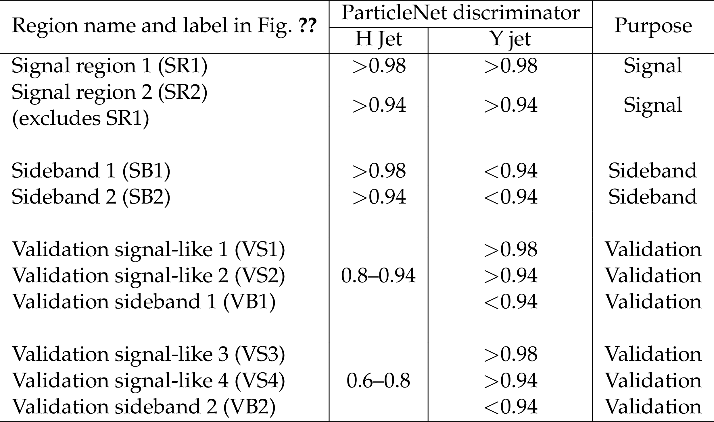
The distributions of the H and the Y candidate jets' ParticleNet scores for the signal with ${M_{\mathrm{X}}} =$ 1600 GeV and ${M_{\mathrm{Y}}} =$ 90 GeV (filled squares) and multijets background (open circles). The grid lines show the different event categories defined using the ParticleNet scores of the two jets. A description of the regions is given in Table 1 and in the text. |
png pdf |
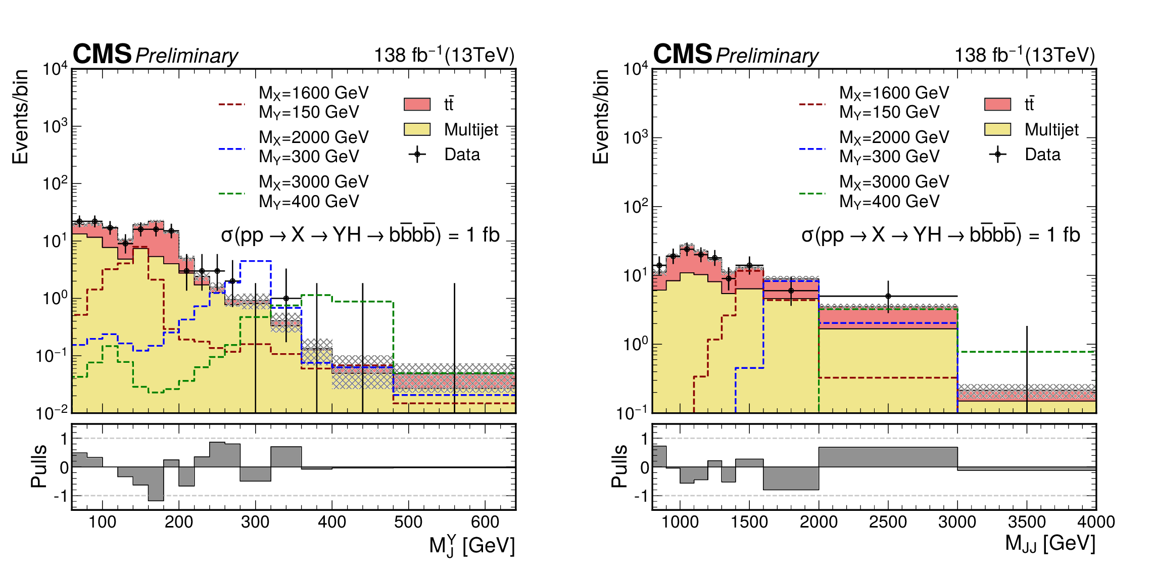
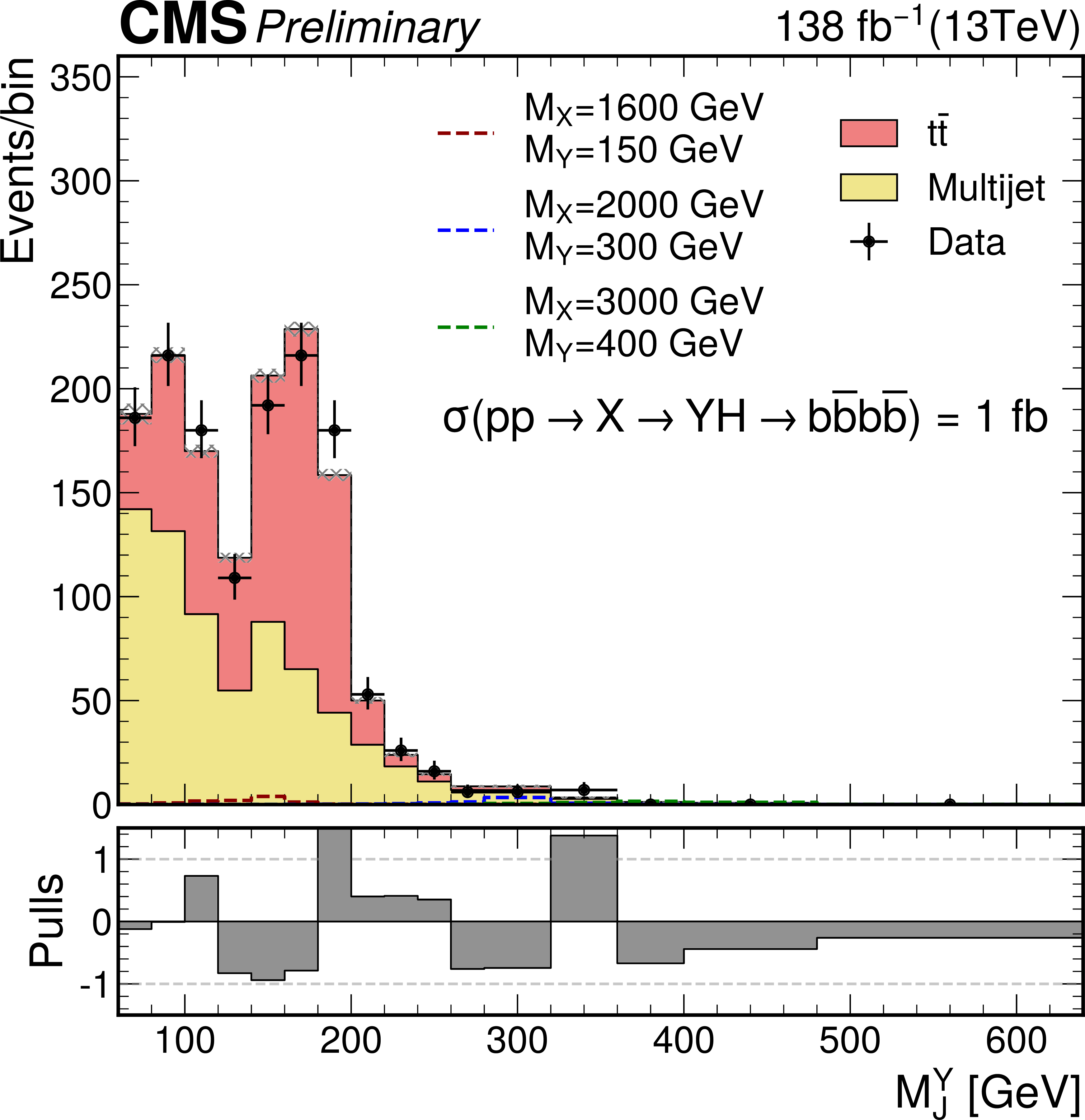
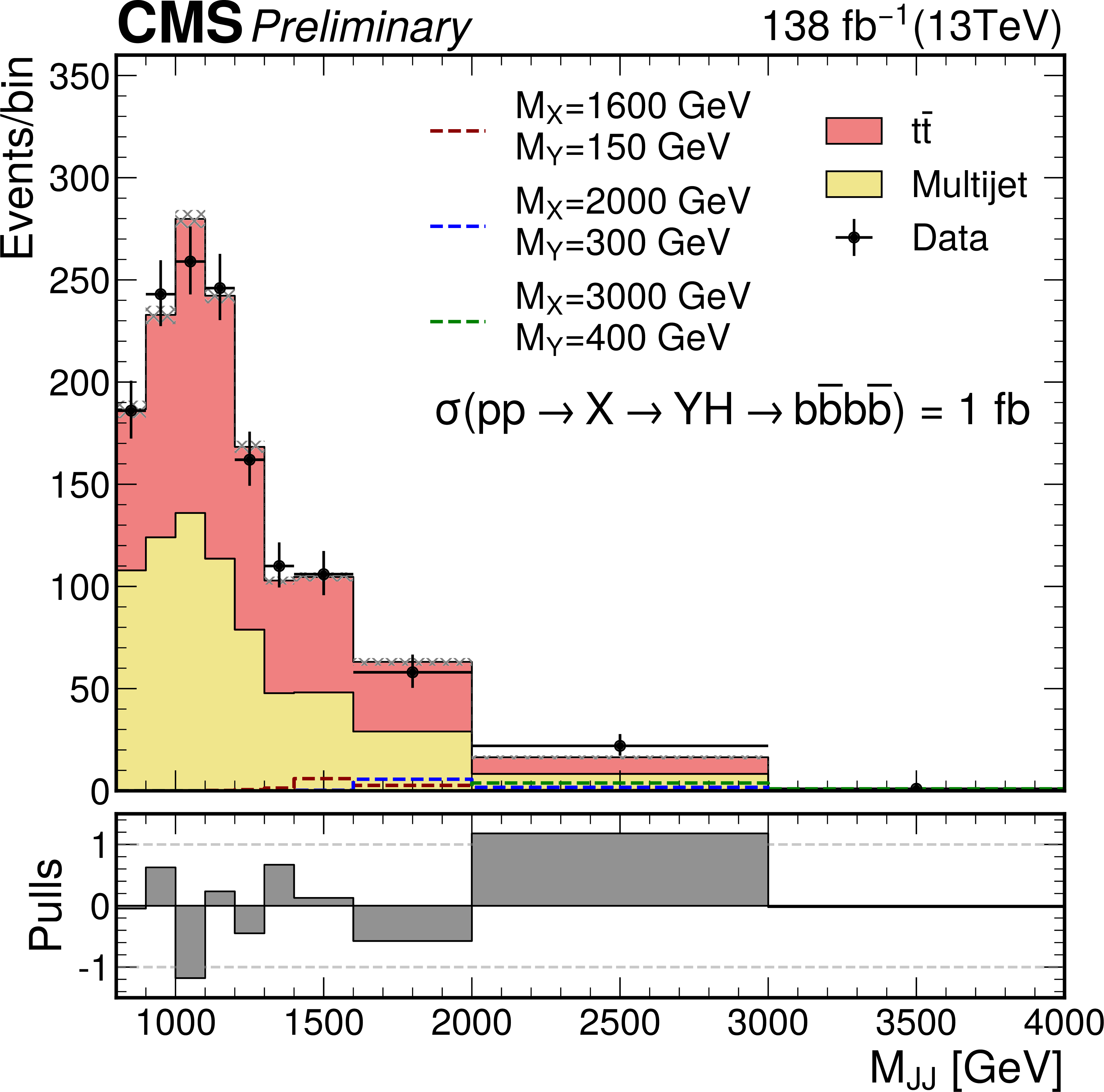
Figure 2:
The $ {M_{\rm J}^{\mathrm{Y}}}$ (left) and ${M_{\rm JJ}}$ (right) distributions for the number of observed events (black markers) compared with the estimated backgrounds (filled histograms) in the signal region 1. The distributions expected from the signal under three ${M_{\mathrm{X}}}$ and ${M_{\mathrm{Y}}}$ hypotheses and assuming a cross section of 1 fb are also shown. The lower panels show the "Pulls'' defined as (observed events$-$expected events)$/\sqrt {\sigma _{obs}^{2} + \sigma _{exp}^{2}}$, where $\sigma _{obs}$ and $\sigma _{exp}$ are the statistical and total uncertainties in the observation and the background estimation, respectively. |
png pdf |
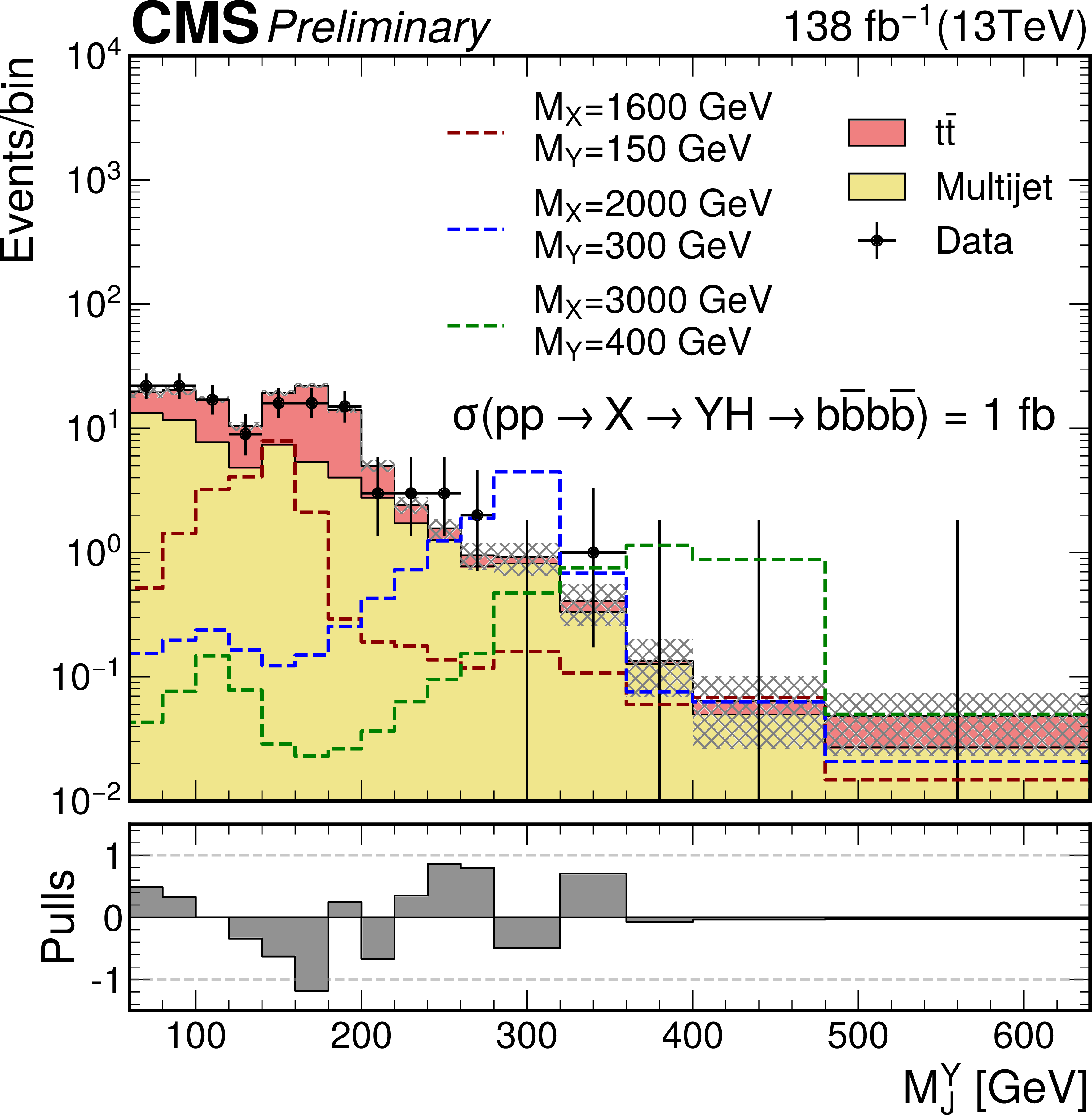
Figure 2-a:
The $ {M_{\rm J}^{\mathrm{Y}}}$ distribution for the number of observed events (black markers) compared with the estimated backgrounds (filled histograms) in the signal region 1. The distributions expected from the signal under three ${M_{\mathrm{X}}}$ and ${M_{\mathrm{Y}}}$ hypotheses and assuming a cross section of 1 fb are also shown. The lower panel shows the "Pulls'' defined as (observed events$-$expected events)$/\sqrt {\sigma _{obs}^{2} + \sigma _{exp}^{2}}$, where $\sigma _{obs}$ and $\sigma _{exp}$ are the statistical and total uncertainties in the observation and the background estimation, respectively. |
png pdf |
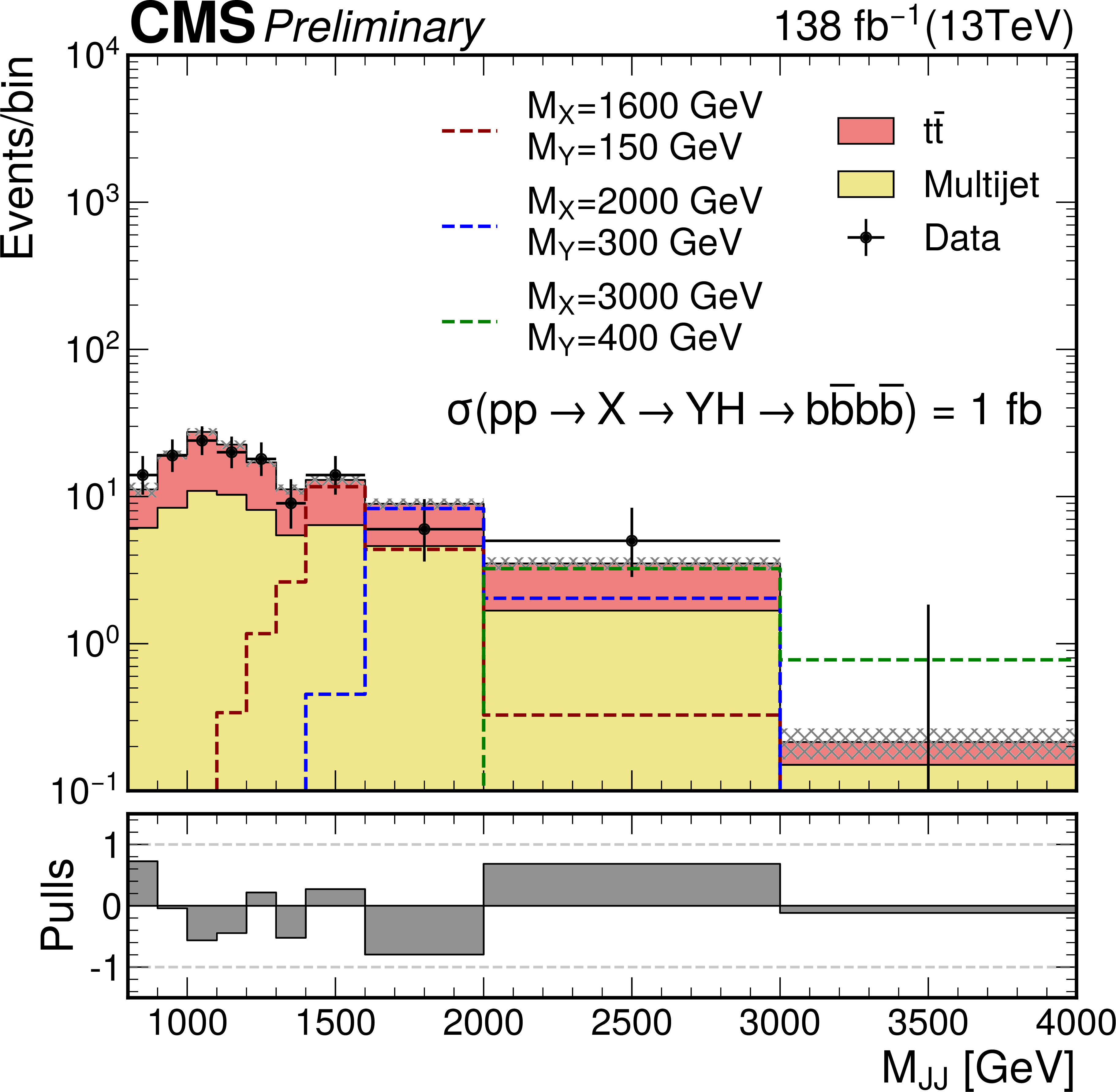
Figure 2-b:
The ${M_{\rm JJ}}$ distribution for the number of observed events (black markers) compared with the estimated backgrounds (filled histograms) in the signal region 1. The distributions expected from the signal under three ${M_{\mathrm{X}}}$ and ${M_{\mathrm{Y}}}$ hypotheses and assuming a cross section of 1 fb are also shown. The lower panel shows the "Pulls'' defined as (observed events$-$expected events)$/\sqrt {\sigma _{obs}^{2} + \sigma _{exp}^{2}}$, where $\sigma _{obs}$ and $\sigma _{exp}$ are the statistical and total uncertainties in the observation and the background estimation, respectively. |

png pdf |
Figure 3:
The 95% confidence level expected (left) and observed (right) upper limits on $\sigma ({\mathrm{p}} {\mathrm{p}} \,\to \, {\mathrm{X} \,\to \,\mathrm{Y} \mathrm{H} \,\to \,\mathrm{b} \mathrm{\bar{b}} \mathrm{b} \mathrm{\bar{b}}})$ for different values of ${M_{\mathrm{X}}}$ and ${M_{\mathrm{Y}}}$. |
png pdf |
Figure 3-a:
The 95% confidence level expected upper limits on $\sigma ({\mathrm{p}} {\mathrm{p}} \,\to \, {\mathrm{X} \,\to \,\mathrm{Y} \mathrm{H} \,\to \,\mathrm{b} \mathrm{\bar{b}} \mathrm{b} \mathrm{\bar{b}}})$ for different values of ${M_{\mathrm{X}}}$ and ${M_{\mathrm{Y}}}$. |
png pdf |
Figure 3-b:
The 95% confidence level observed upper limits on $\sigma ({\mathrm{p}} {\mathrm{p}} \,\to \, {\mathrm{X} \,\to \,\mathrm{Y} \mathrm{H} \,\to \,\mathrm{b} \mathrm{\bar{b}} \mathrm{b} \mathrm{\bar{b}}})$ for different values of ${M_{\mathrm{X}}}$ and ${M_{\mathrm{Y}}}$. |
| Tables | |
png pdf |
Table 1:
Definition of the signal, sideband, and validation regions used for background estimation. The regions are defined in terms of the ParticleNet discriminators of the H and Y candidate jets, as shown in Fig. 1. |
| Summary |
| A search for massive scalar resonances X and Y, where X decays to the lighter Y and the standard model Higgs boson H, is conducted in LHC proton-proton collision data collected by the CMS detector between 2016 and 2018 and corresponding to an integrated luminosity of 138 fb$^{-1}$. The considered decay modes of both Y and H are to a b quark-antiquark pairs each. Events are selected assuming very high Lorentz-boost of both the Y and the H, for which specialized jet substructure and identification techniques are used. The background, composed of multijets and $\mathrm{t\bar{t}}$, is estimated using data control samples and Monte Carlo simulations. A binned likelihood fit to the data is performed using the reconstructed mass distributions of the X and Y candidates. Upper limits are set on the cross section of the process $\mathrm{X} \,\,\to\,\, \mathrm{Y} \mathrm{H} \,\,\to\,\, \mathrm{b\bar{b}}\mathrm{b\bar{b}}$ for assumed masses of X in the range 0.9-4 TeV and Y between 60-600 GeV. The results are interpreted in the context of the next-to-minimal supersymmetric standard model (NMSSM) scalar sector. This search significantly extends limit ranges of NMSSM scalars over previous analyses and places the most stringent cross section limits over much of the explored X and Y mass ranges to date. |
| Additional Figures | |
png pdf |
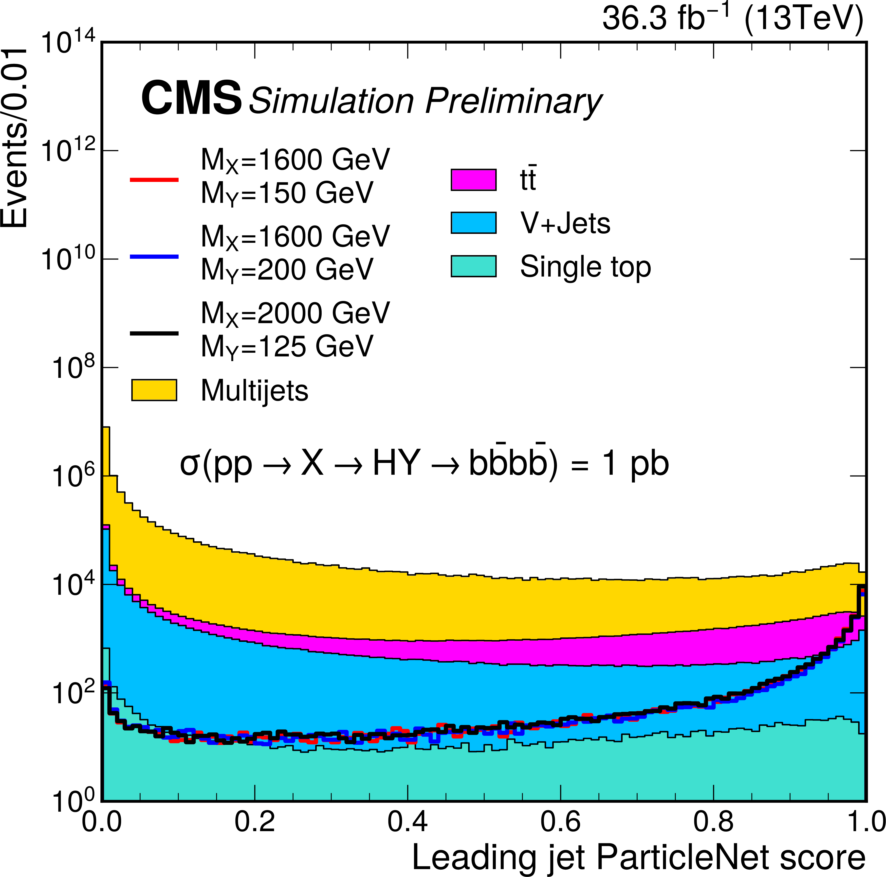
Additional Figure 1:
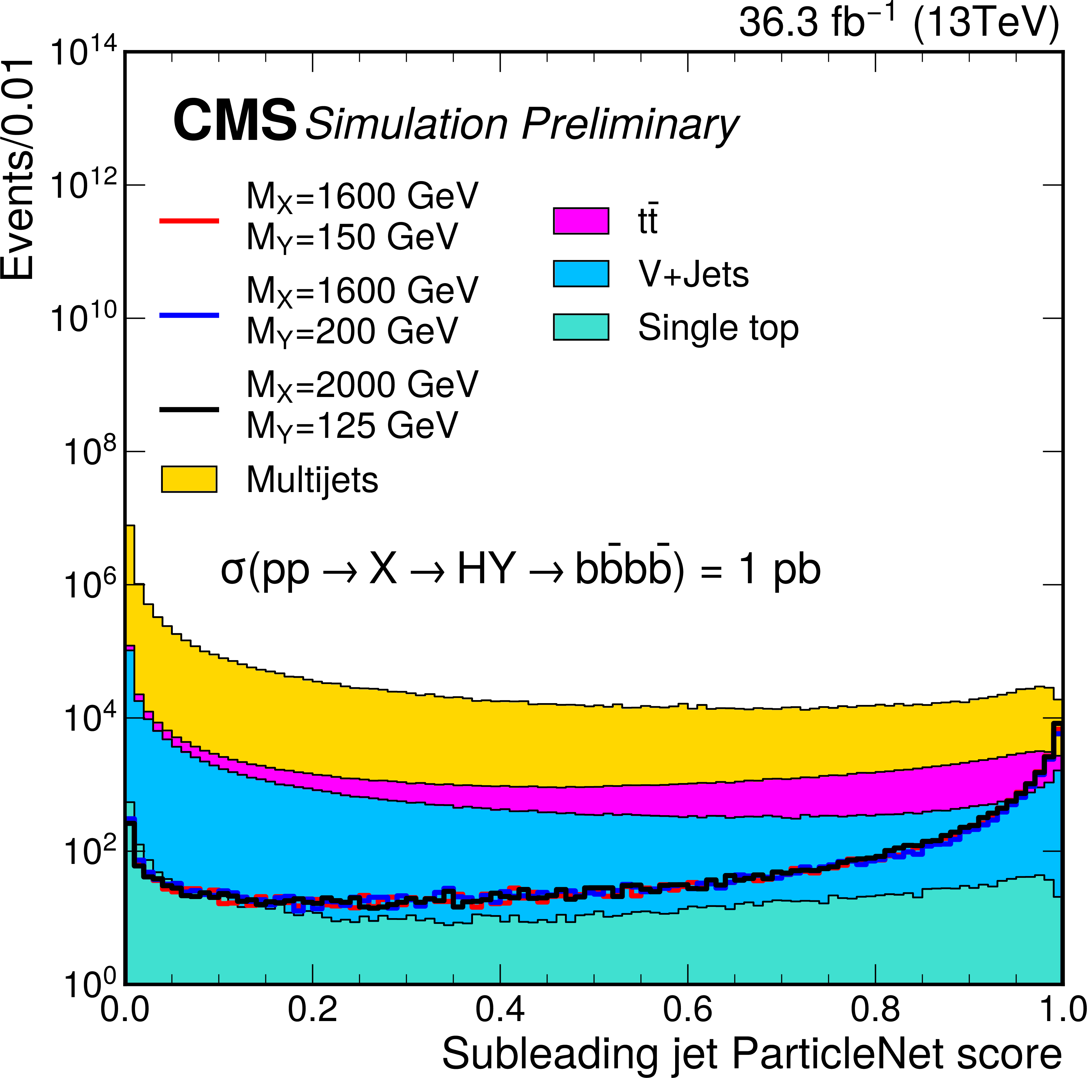
The ParticleNet score of the leading $p_{\mathrm{T}}$ AK8 jet in 2016 simulations. The filled histograms show the various standard model background processes and the lines show the signal for three different mass hypotheses of the X and Y resonances. The main backgrounds are the standard model multijet and ${{\mathrm {t}\overline {\mathrm {t}}}} $+jets processes. The minor backgrounds are the V+jets (V= W and Z) and single top production, which are not estimated separately from the multijets background. |

png pdf |
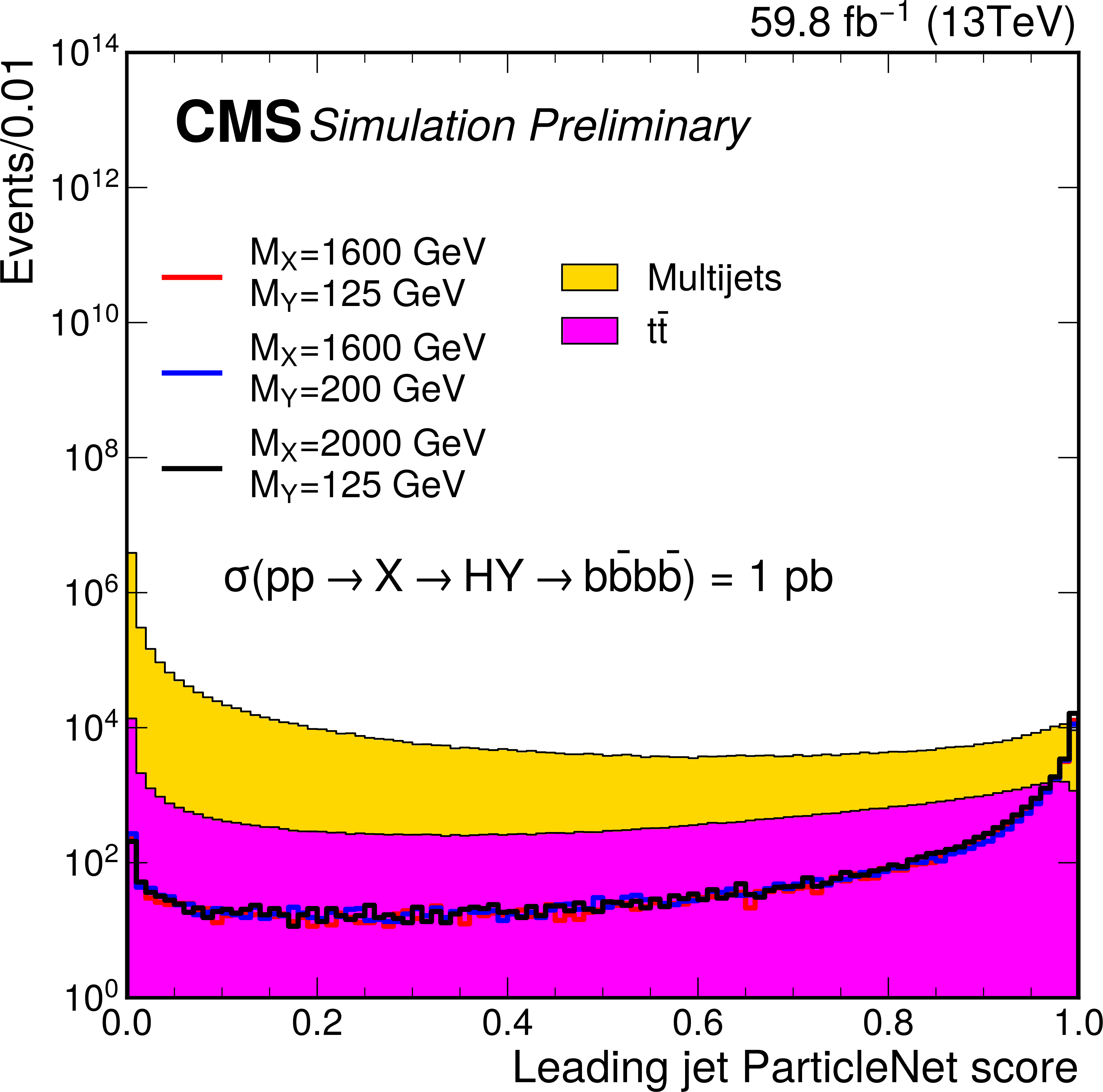
Additional Figure 2:
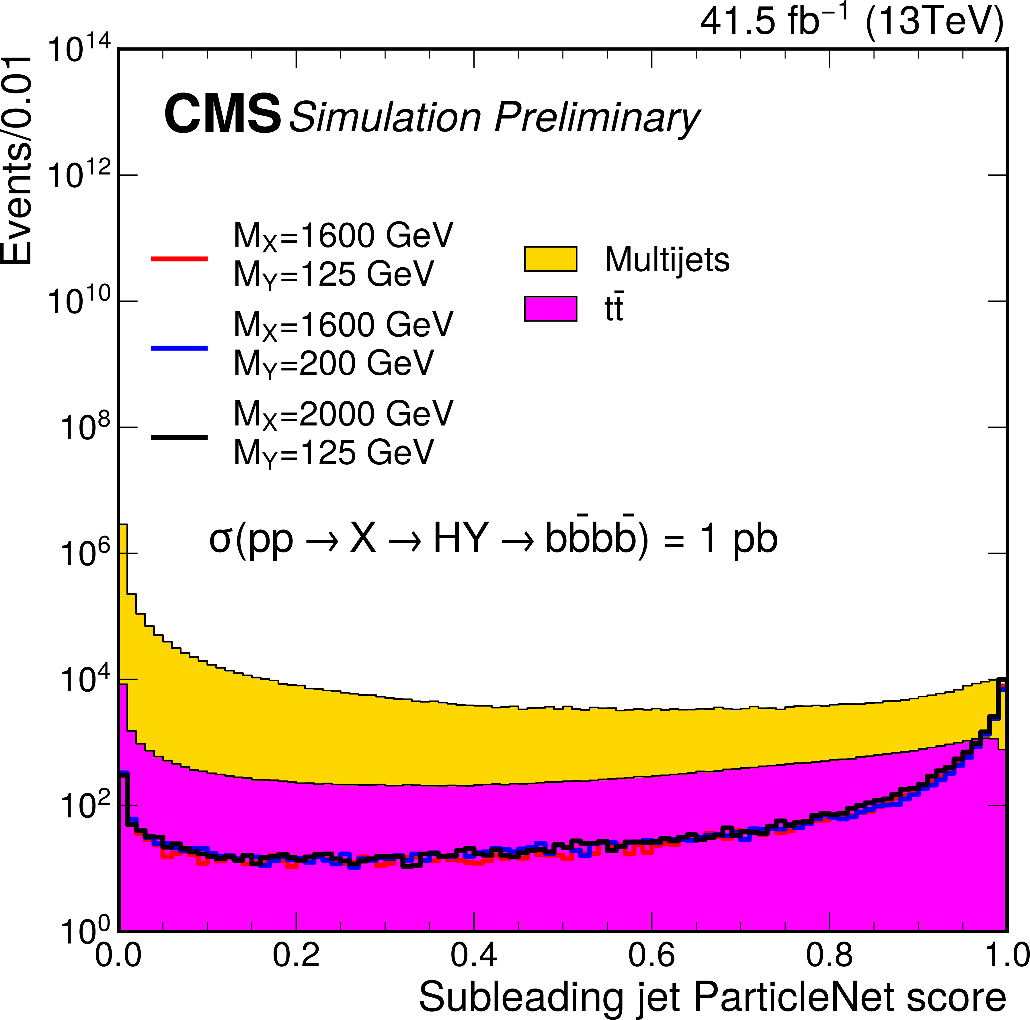
The ParticleNet score of the leading $p_{\mathrm{T}}$ AK8 jet in 2017 simulations. The filled histograms show the main backgrounds, the standard model multijet and ${{\mathrm {t}\overline {\mathrm {t}}}} $+jets processes. The lines show the signal for three different mass hypotheses of the X and Y resonances. |
png pdf |
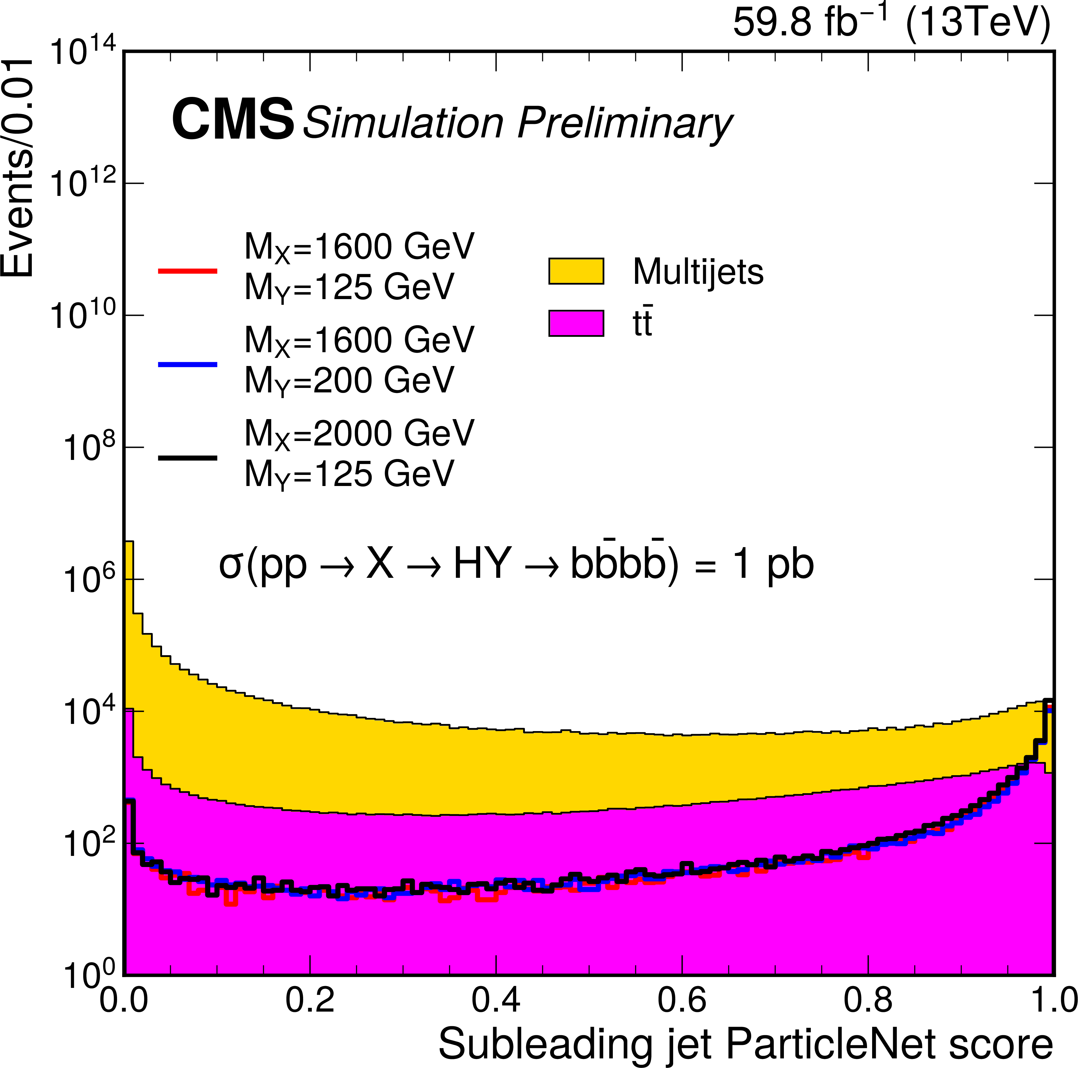
Additional Figure 3:
The ParticleNet score of the leading $p_{\mathrm{T}}$ AK8 jet in 2018 simulations. The filled histograms show the main backgrounds, the standard model multijet and ${{\mathrm {t}\overline {\mathrm {t}}}} $+jets processes. The lines show the signal for three different mass hypotheses of the X and Y resonances. |
png pdf |
Additional Figure 4:
The ParticleNet score of the second-leading $p_{\mathrm{T}}$ AK8 jet in 2016 simulations. The filled histograms show the various standard model background processes and the lines show the signal for three different mass hypotheses of the X and Y resonances. The main backgrounds are the standard model multijet and ${{\mathrm {t}\overline {\mathrm {t}}}} $+jets processes. The minor backgrounds are the V+jets (V= W and Z) and single top production, which are not estimated separately from the multijets background. |
png pdf |
Additional Figure 5:
The ParticleNet score of the second-leading $p_{\mathrm{T}}$ AK8 jet in 2017 simulations. The filled histograms show the main backgrounds, the standard model multijet and ${{\mathrm {t}\overline {\mathrm {t}}}} $+jets processes. The lines show the signal for three different mass hypotheses of the X and Y resonances. |
png pdf |
Additional Figure 6:
The ParticleNet score of the second-leading $p_{\mathrm{T}}$ AK8 jet in 2018 simulations. The filled histograms show the main backgrounds, the standard model multijet and ${{\mathrm {t}\overline {\mathrm {t}}}} $+jets processes. The lines show the signal for three different mass hypotheses of the X and Y resonances. |
png pdf |
Additional Figure 7:
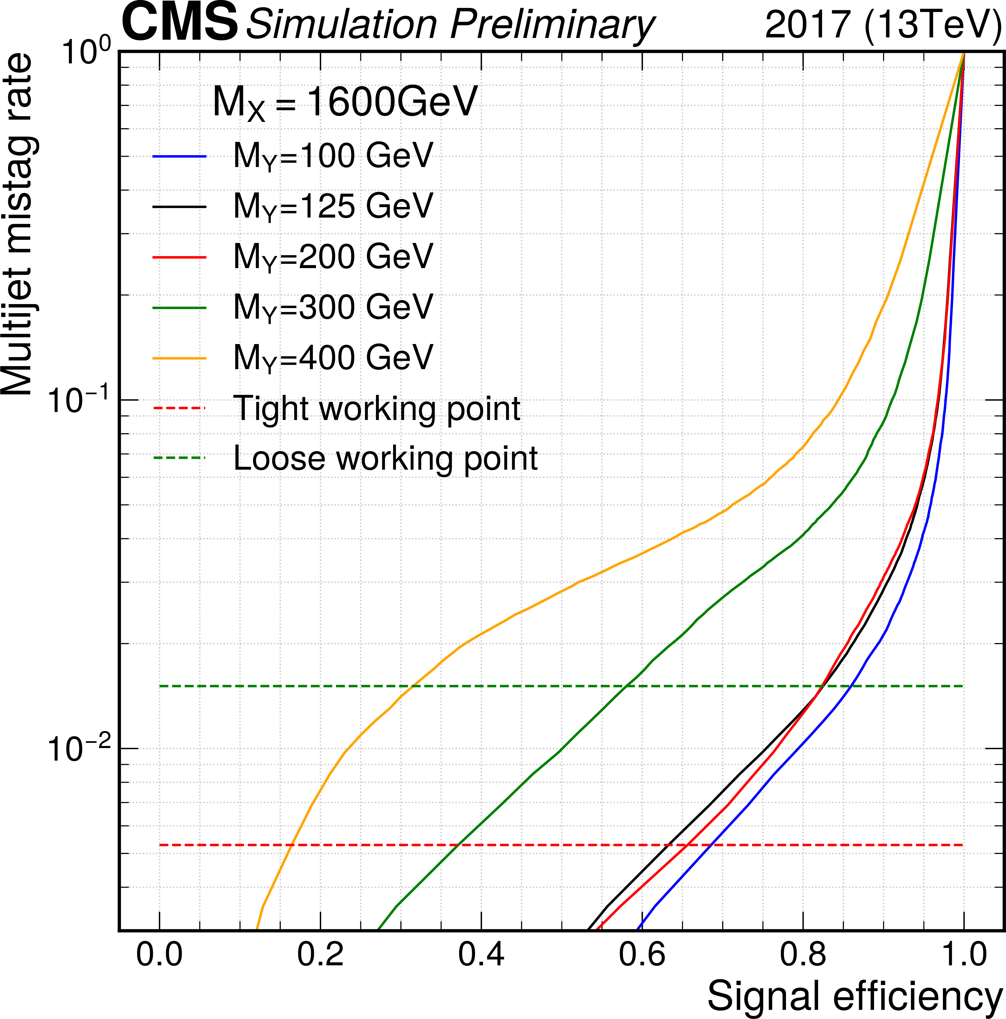
The ParticleNet ROC curves in 2017 simulations for $M_{\mathrm{X}}$=1600 GeV and different mass hypotheses of the Y resonance. The horizontal dashed lines show the mistag rates for tight and loose working points. |
png pdf |
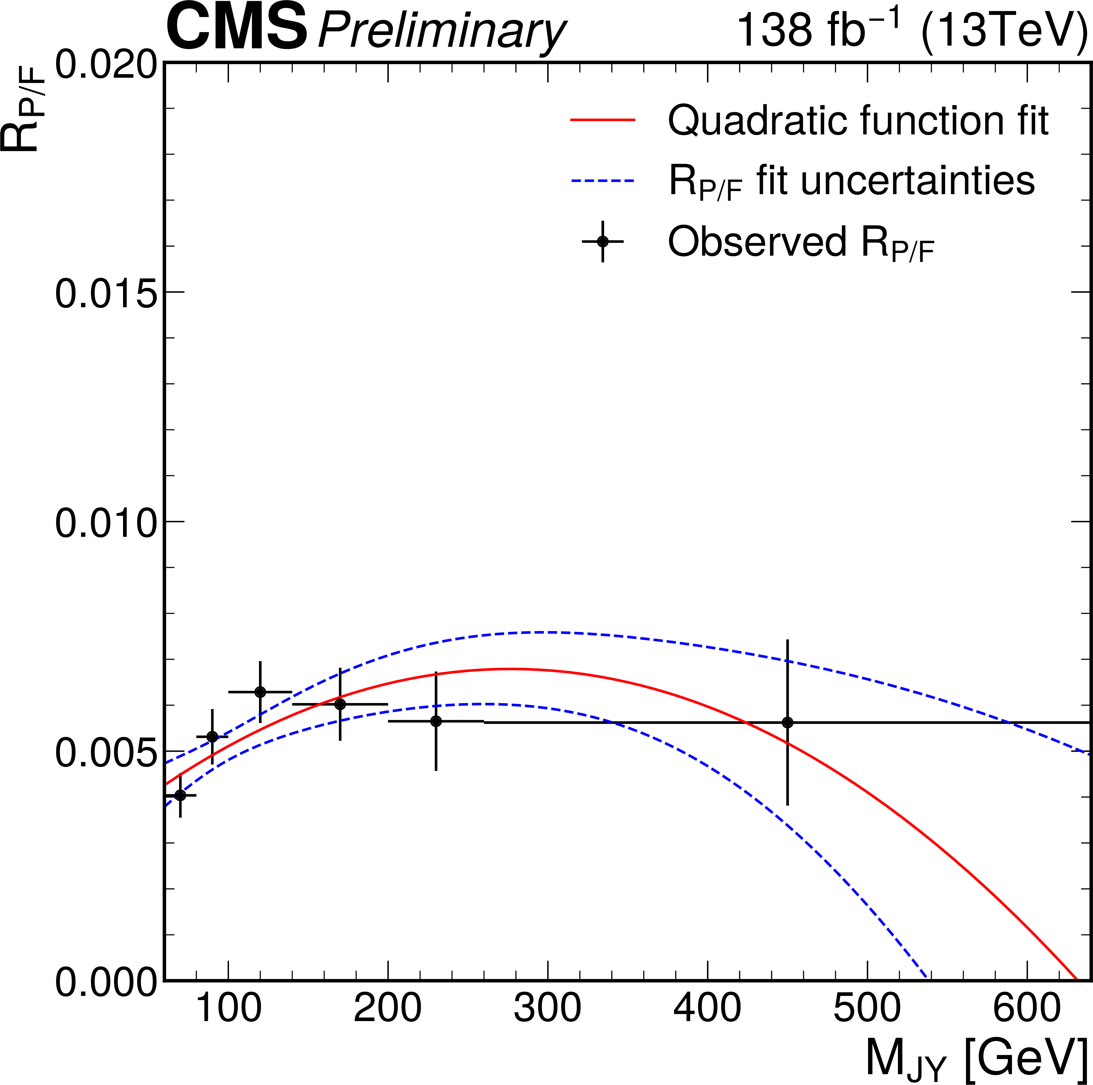
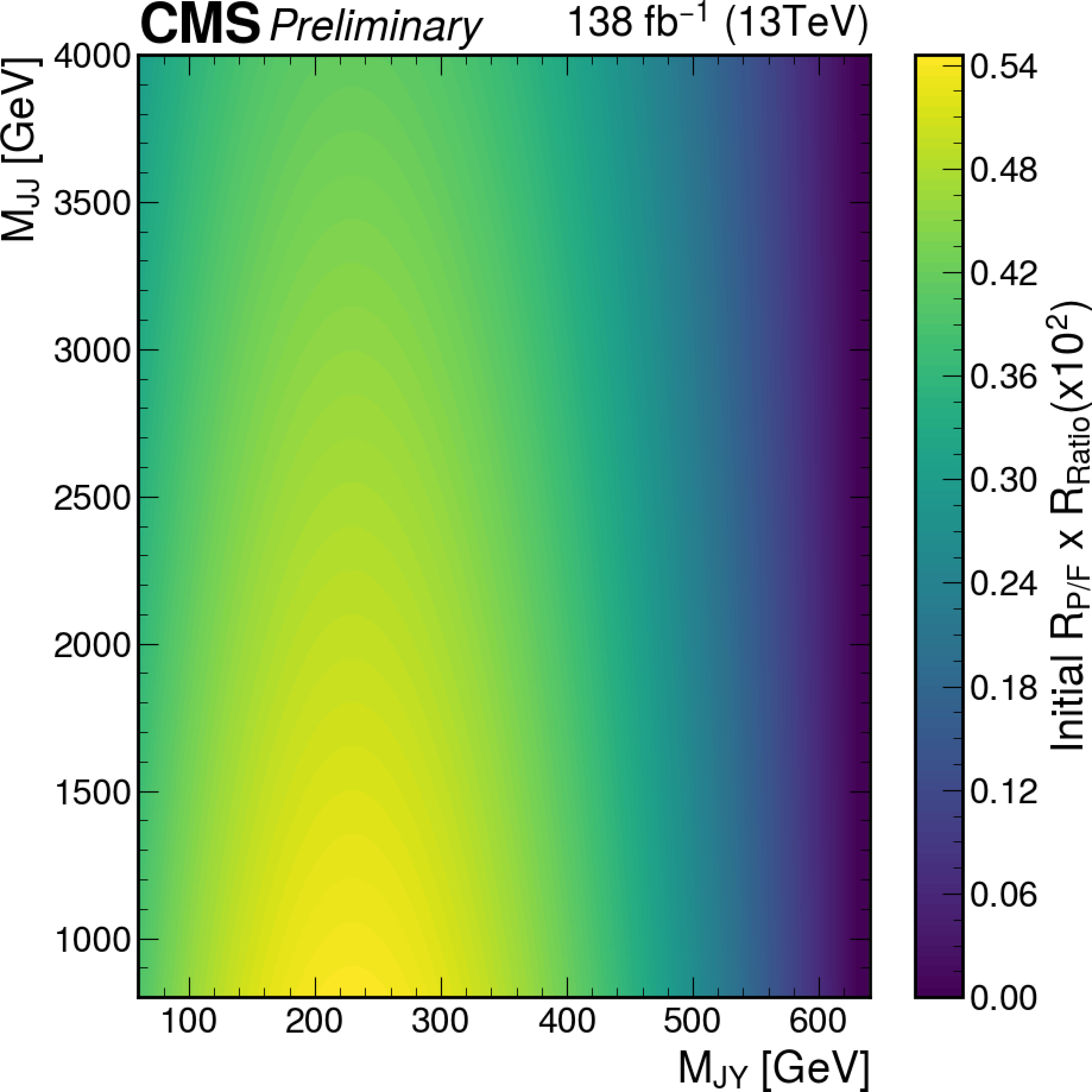
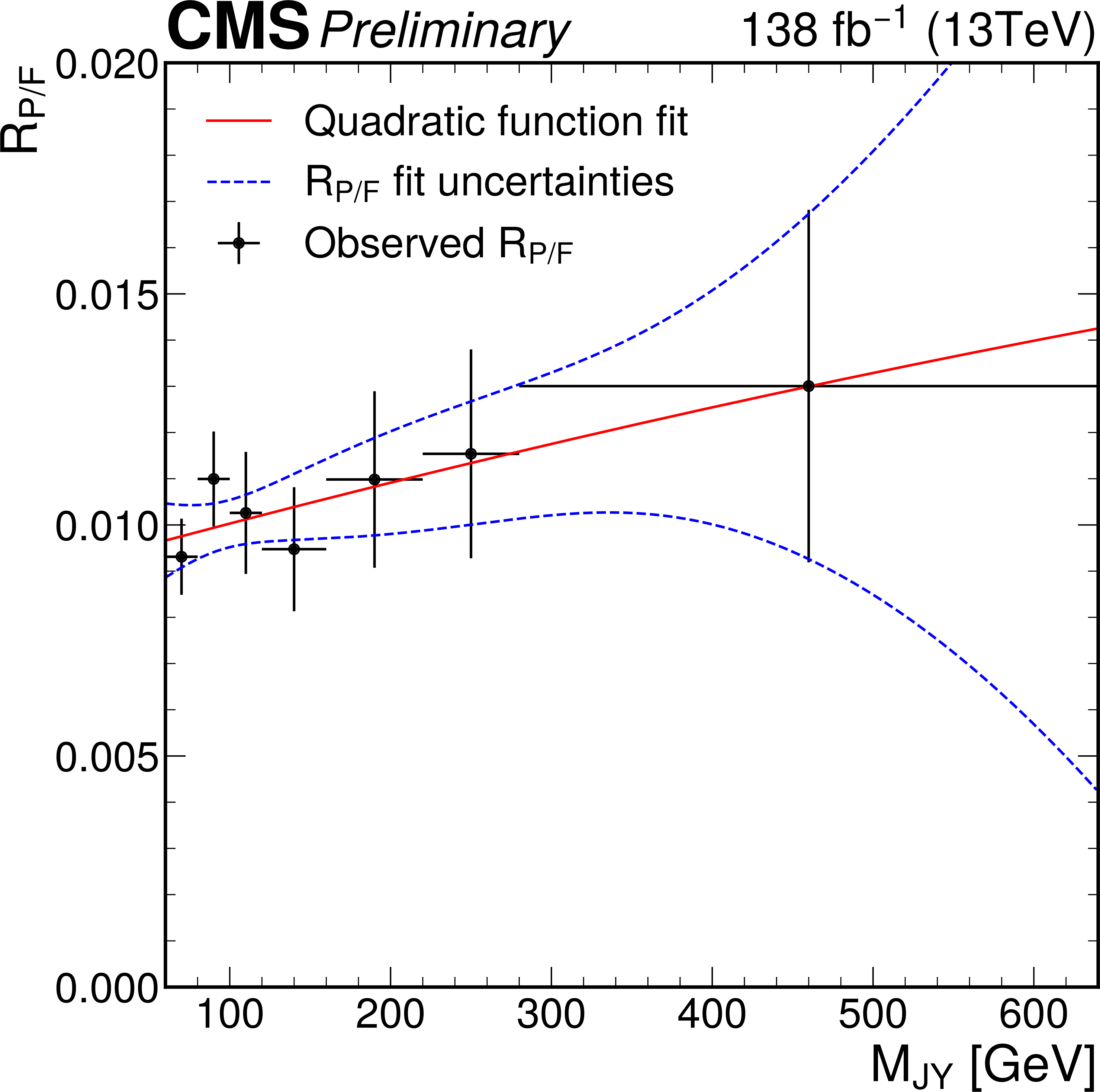
Additional Figure 8:
Initial $R_{P/F}$ measured for the VS3 and VB2 region in the full RunII data and used in the validation fit. Simulation prediction of the $\mathrm{t\bar{t}}$ distribution is subtracted from the combined observe data and a second order polynomial is fitted to the result. |
png pdf |
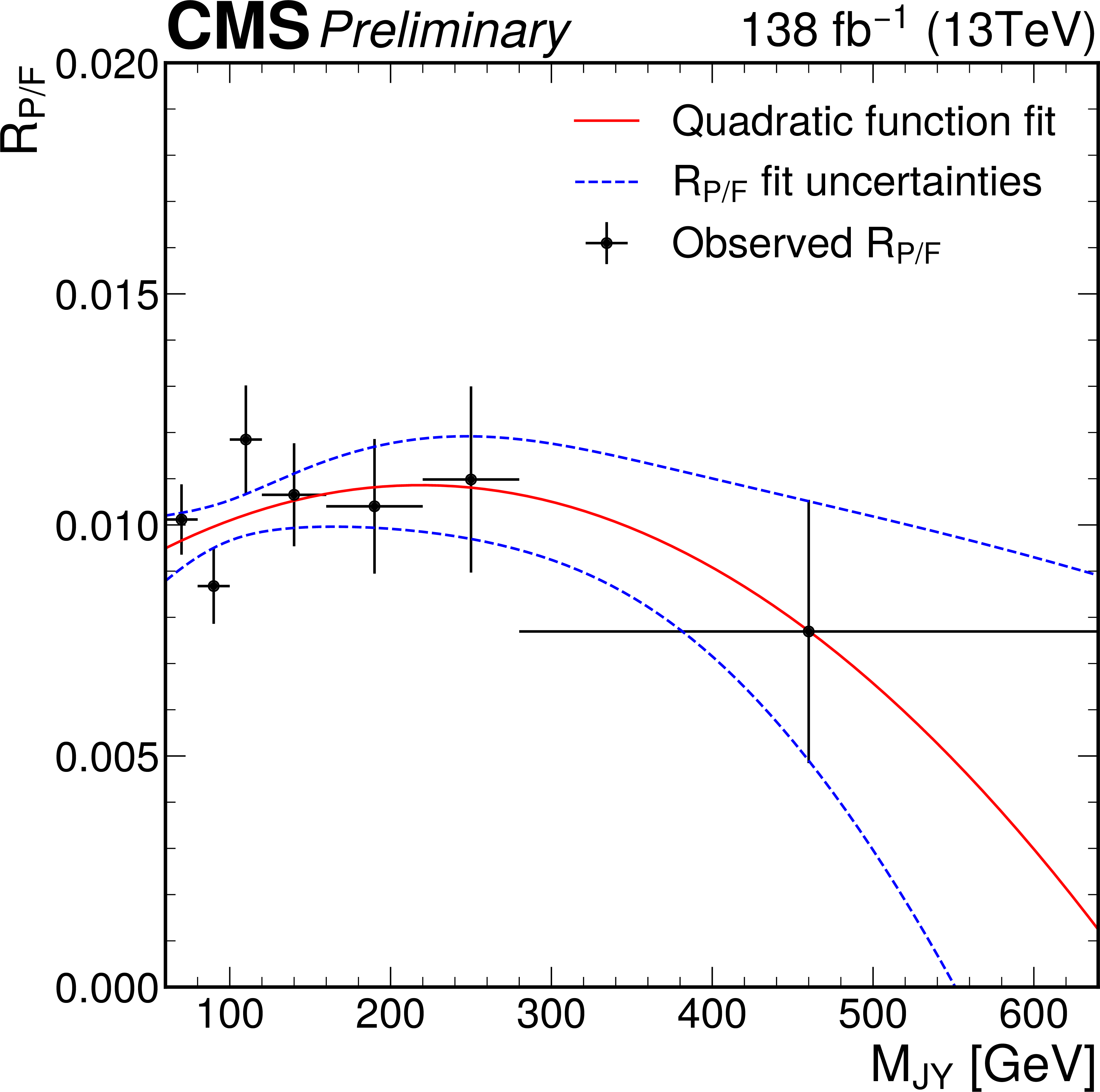
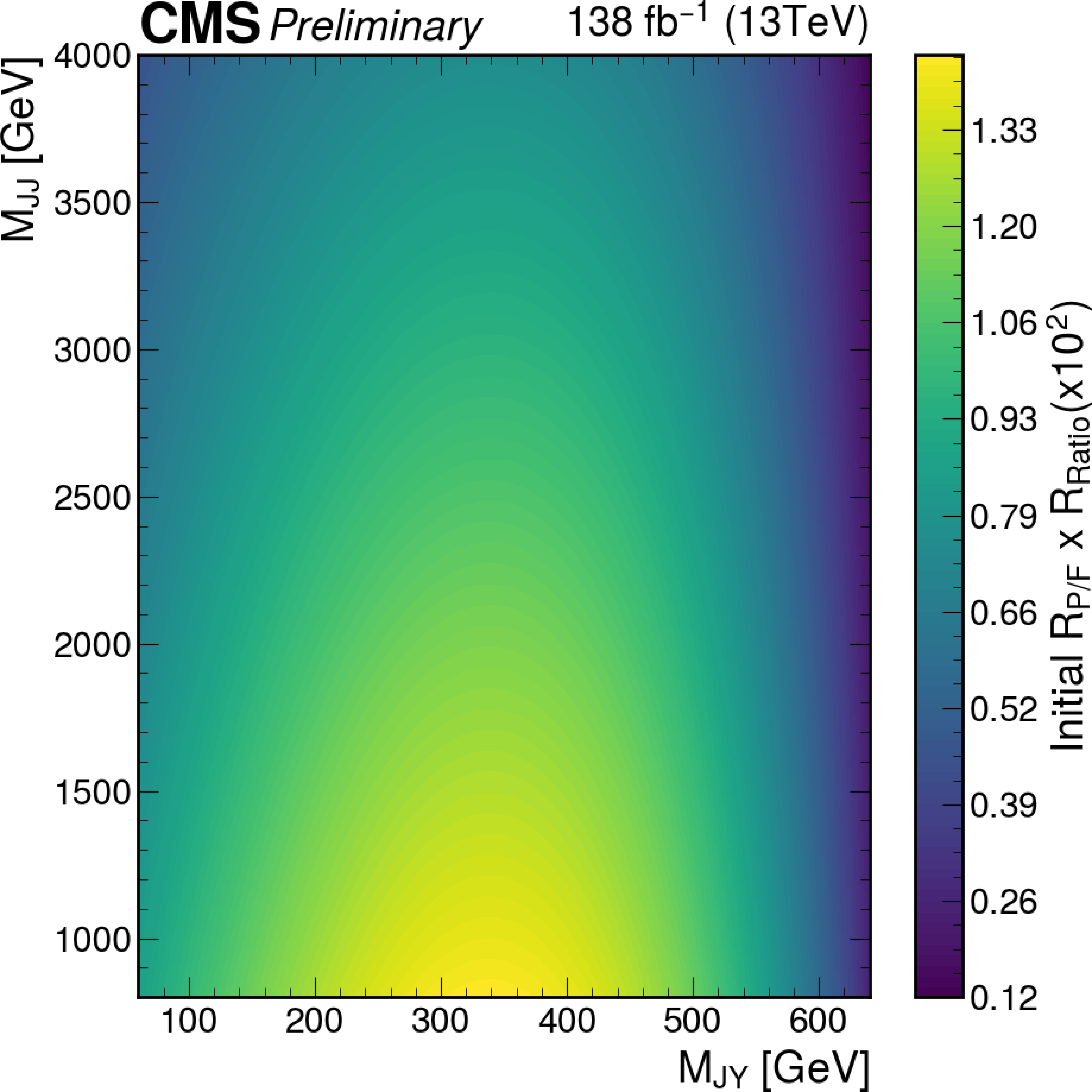
Additional Figure 9:
Initial $R_{P/F}$ measured for the VS4 and VB2 region in the full RunII data and used in the validation fit. Simulation prediction of the $\mathrm{t\bar{t}}$ distribution is subtracted from the combined observe data and a second order polynomial is fitted to the result. |
png pdf |
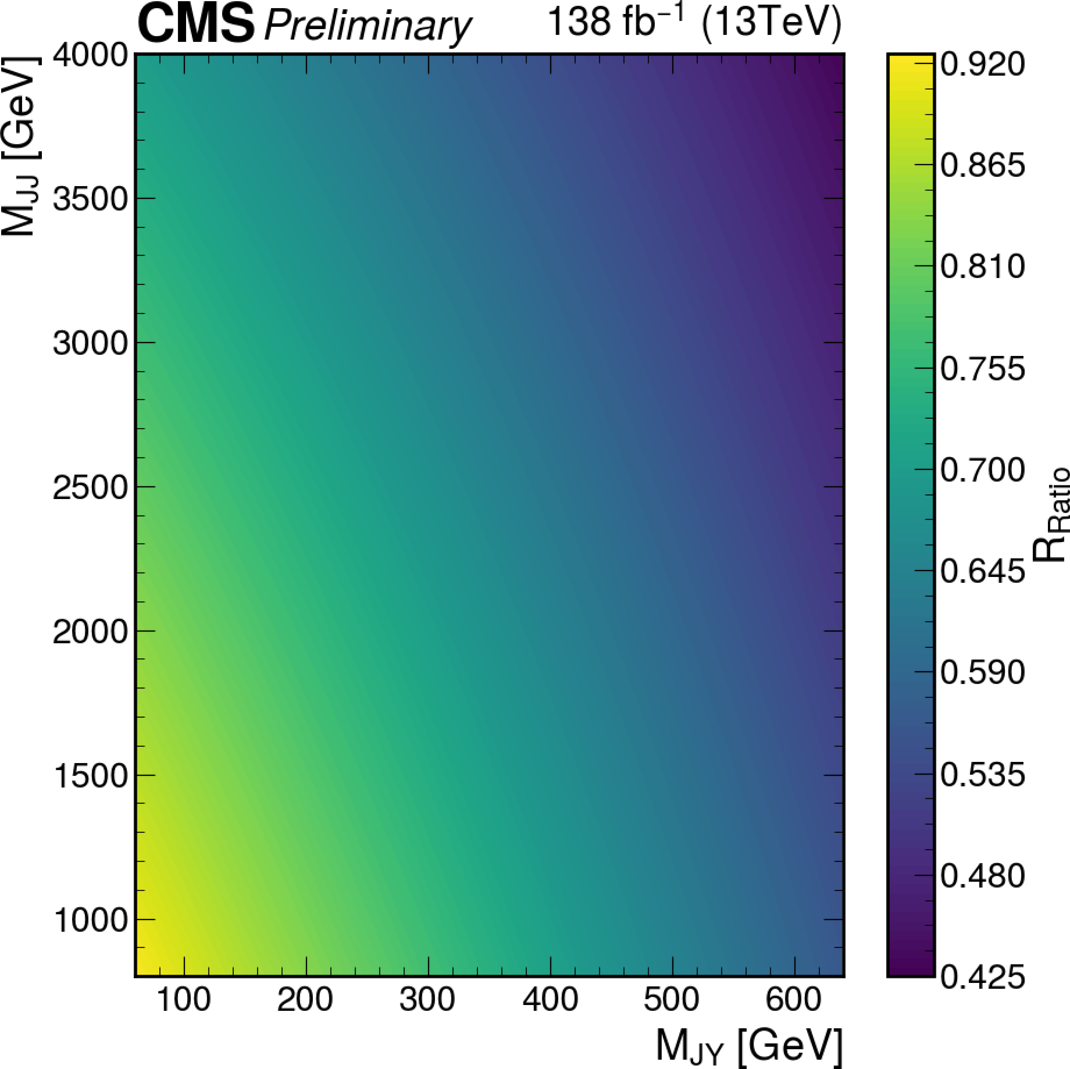
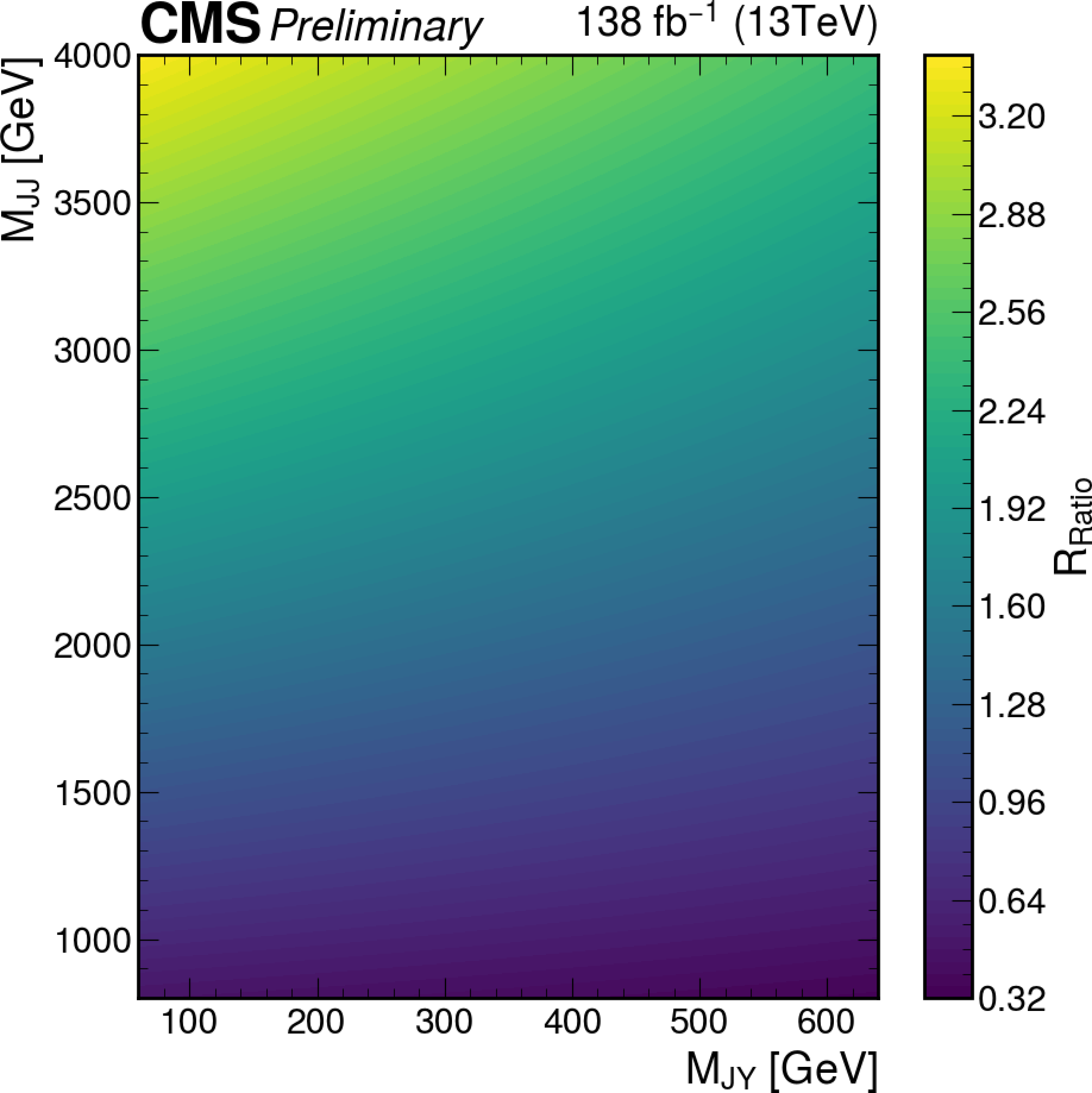
Additional Figure 10:
The $R_{\text{Ratio}}$ for the VS1 after the validation fit. |
png pdf |
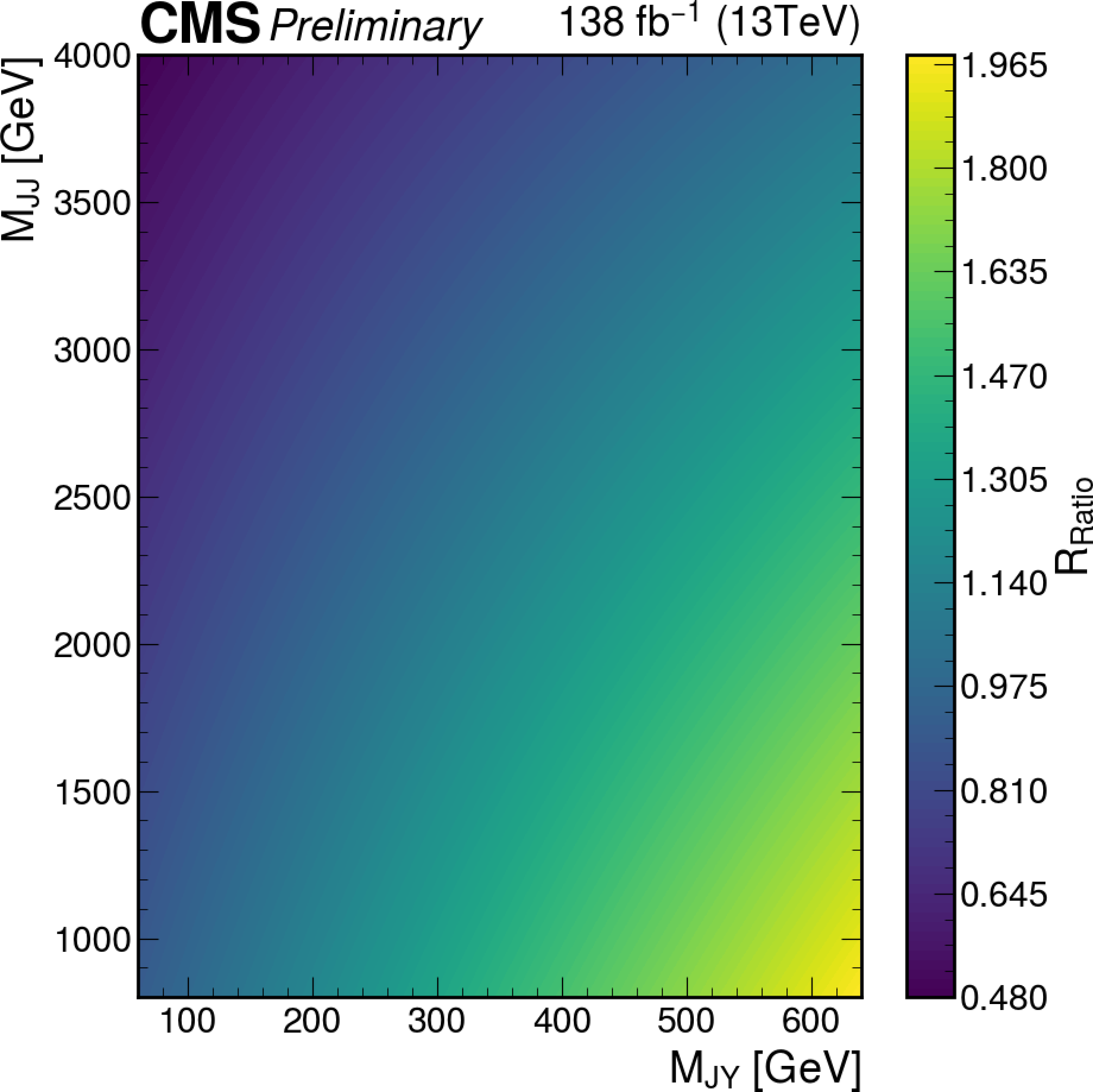
Additional Figure 11:
The $R_{\text{Ratio}}$ for the VS2 after the validation fit. |
png pdf |
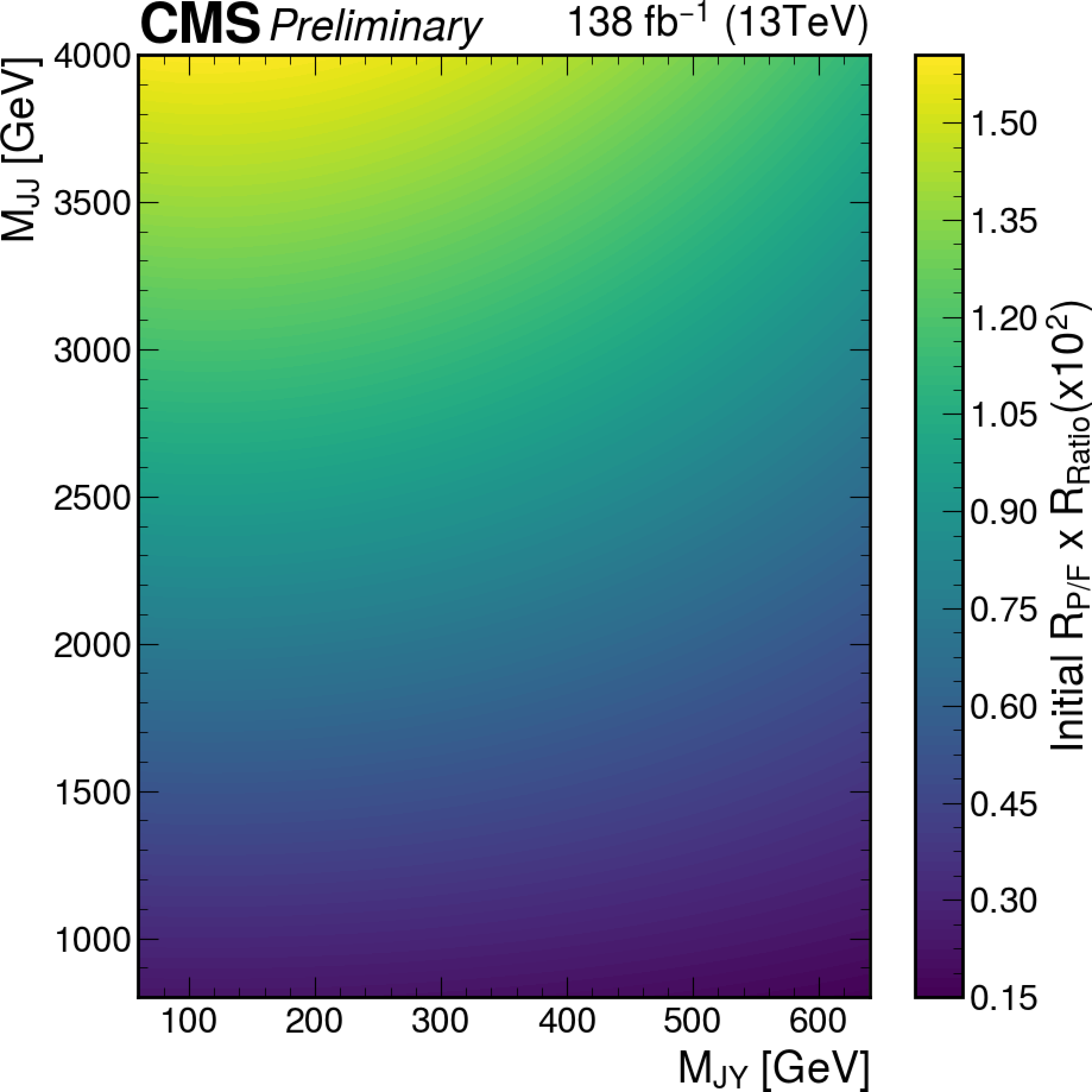
Additional Figure 12:
The final transfer function, $R_{P/F}^{\text{init}}\times R_{\text{Ratio}}$, in the VS1 after the validation fit. |
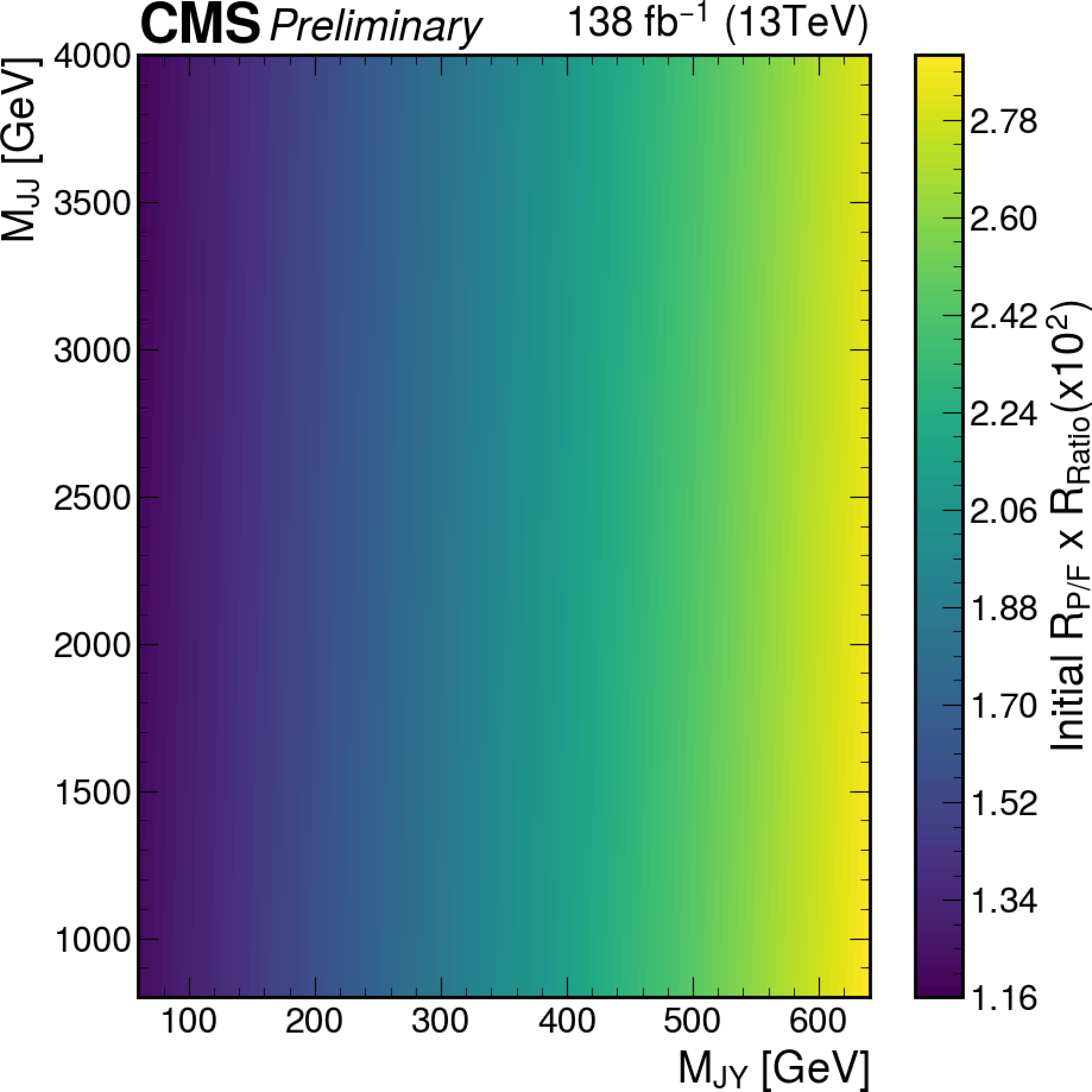
png pdf |
Additional Figure 13:
The final transfer function, $R_{P/F}^{\text{init}}\times R_{\text{Ratio}}$, in the VS2 after the validation fit. |
png pdf |
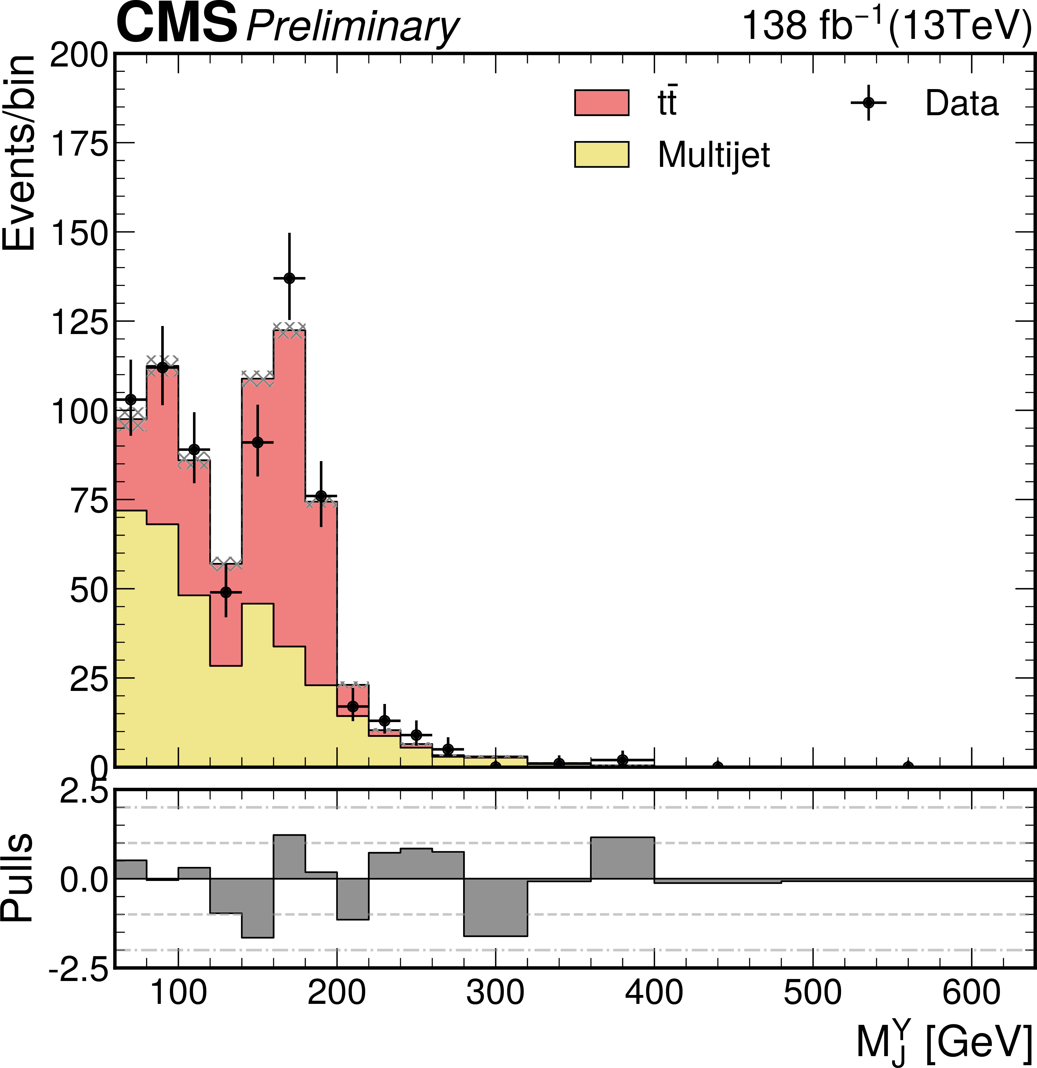
Additional Figure 14:
The $M_{\mathrm{JY}}$ distribution for the number of observed events (black markers) compared with the estimated backgrounds (filled histograms) in the validation signal-like region 1. |

png pdf |
Additional Figure 15:
The $M_{\mathrm{JJ}}$ distribution for the number of observed events (black markers) compared with the estimated backgrounds (filled histograms) in the validation signal-like region 1. |
png pdf |
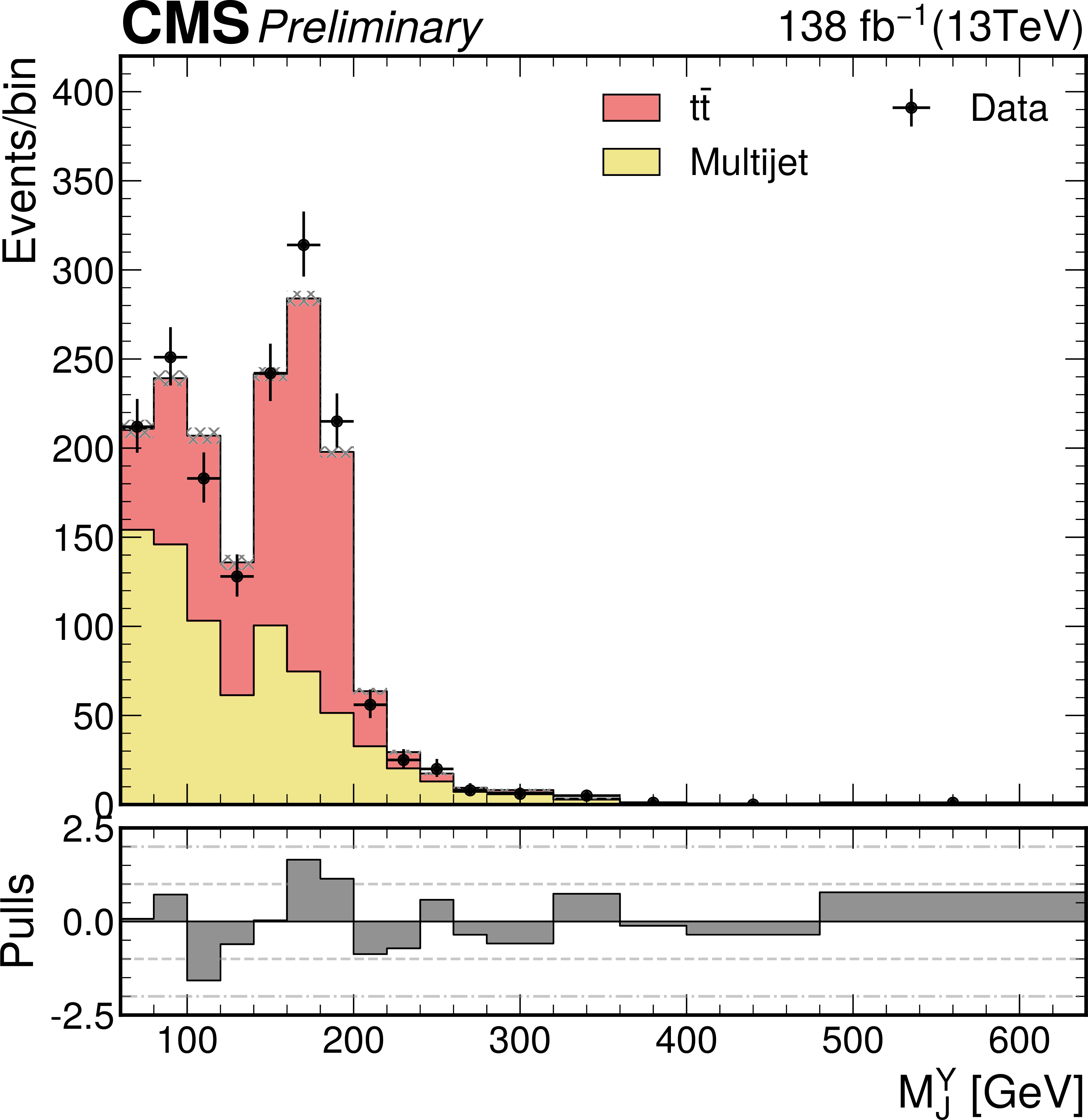
Additional Figure 16:
The $M_{\mathrm{JY}}$ distribution for the number of observed events (black markers) compared with the estimated backgrounds (filled histograms) in the validation signal-like region 2. |

png pdf |
Additional Figure 17:
The $M_{\mathrm{JJ}}$ distribution for the number of observed events (black markers) compared with the estimated backgrounds (filled histograms) in the validation signal-like region 2. |

png pdf |
Additional Figure 18:
Initial $R_{P/F}$ measured for the VS1 and VB1 region in the full RunII data and used in the signal region fit. Simulation prediction of the $\mathrm{t\bar{t}}$ distribution is subtracted from the combined observe data and a second order polynomial is fitted to the result. |
png pdf |
Additional Figure 19:
Initial $R_{P/F}$ measured for the VS2 and VB1 region in the full RunII data and used in the signal region fit. Simulation prediction of the $\mathrm{t\bar{t}}$ distribution is subtracted from the combined observe data and a second order polynomial is fitted to the result. |
png pdf |
Additional Figure 20:
The $R_{\text{Ratio}}$ for the SR1 after the validation fit. |

png pdf |
Additional Figure 21:
The $R_{\text{Ratio}}$ for the SR2 after the validation fit. |
png pdf |
Additional Figure 22:
The final transfer function, $R_{P/F}^{\text{init}}\times R_{\text{Ratio}}$, in the SR1 after the validation fit. |
png pdf |
Additional Figure 23:
The final transfer function, $R_{P/F}^{\text{init}}\times R_{\text{Ratio}}$, in the SR1 after the validation fit. |
png pdf |
Additional Figure 24:
The $M_{\mathrm{JY}}$ distribution for the number of observed events (black markers) compared with the estimated backgrounds (filled histograms) in the validation signal region 2. The distributions expected from the signal under three $M_{\mathrm{X}}$ and $M_{\mathrm{Y}}$ hypotheses and assuming a cross section of 1 fb are also shown. |
png pdf |
Additional Figure 25:
The $M_{\mathrm{JJ}}$ distribution for the number of observed events (black markers) compared with the estimated backgrounds (filled histograms) in the validation signal region 2. The distributions expected from the signal under three $M_{\mathrm{X}}$ and $M_{\mathrm{Y}}$ hypotheses and assuming a cross section of 1 fb are also shown. |
png pdf |
Additional Figure 26:
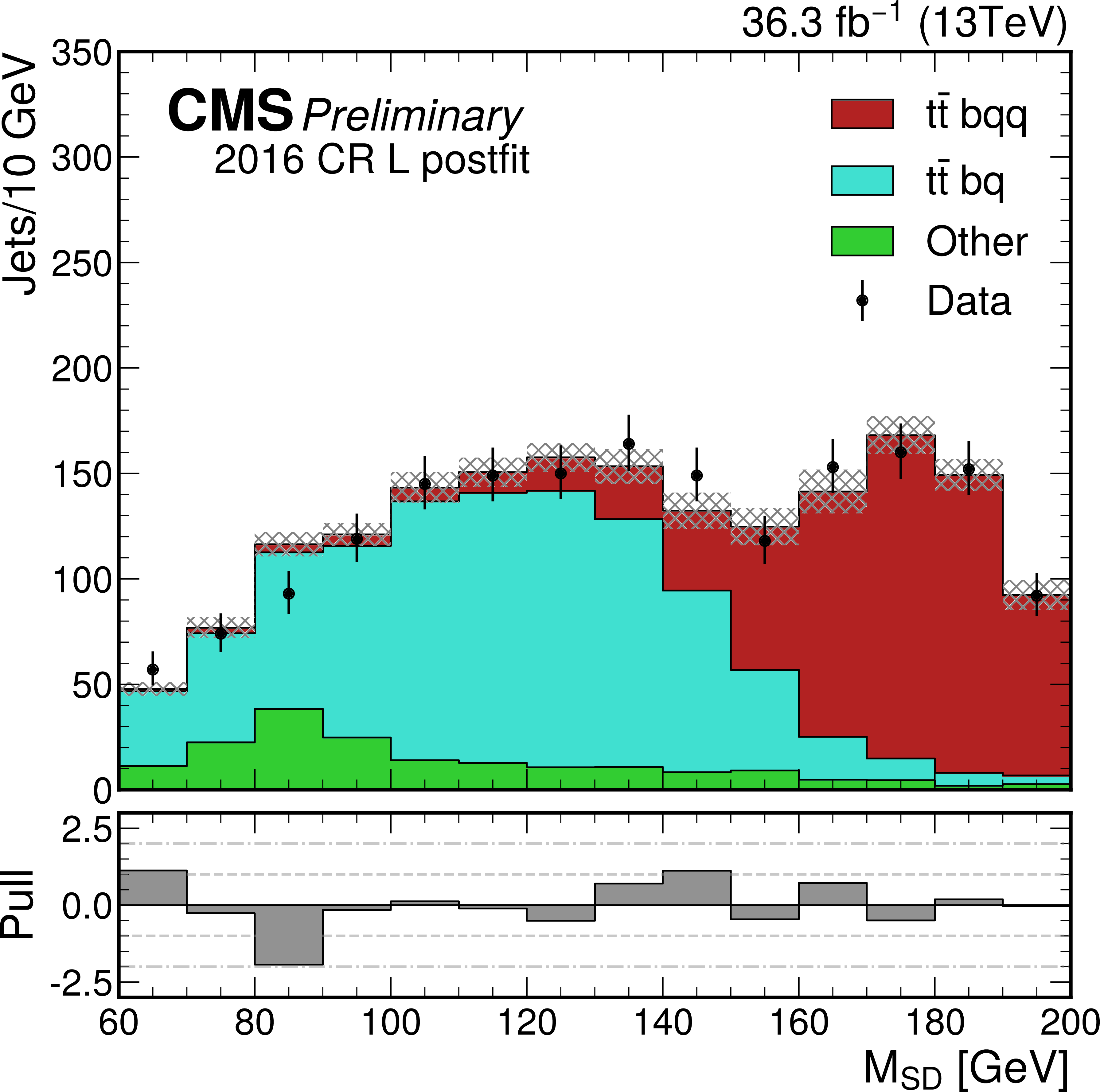
The softdrop mass distribution of the top-quark candidate jets in the 2016 semileptonic control region, loose ParticleNet category (CR L), after the joint semileptonic and hadronic signal region fit. Observed data (black markers) and the postfit estimate (filled histograms) are shown for the three jet categories. |
png pdf |
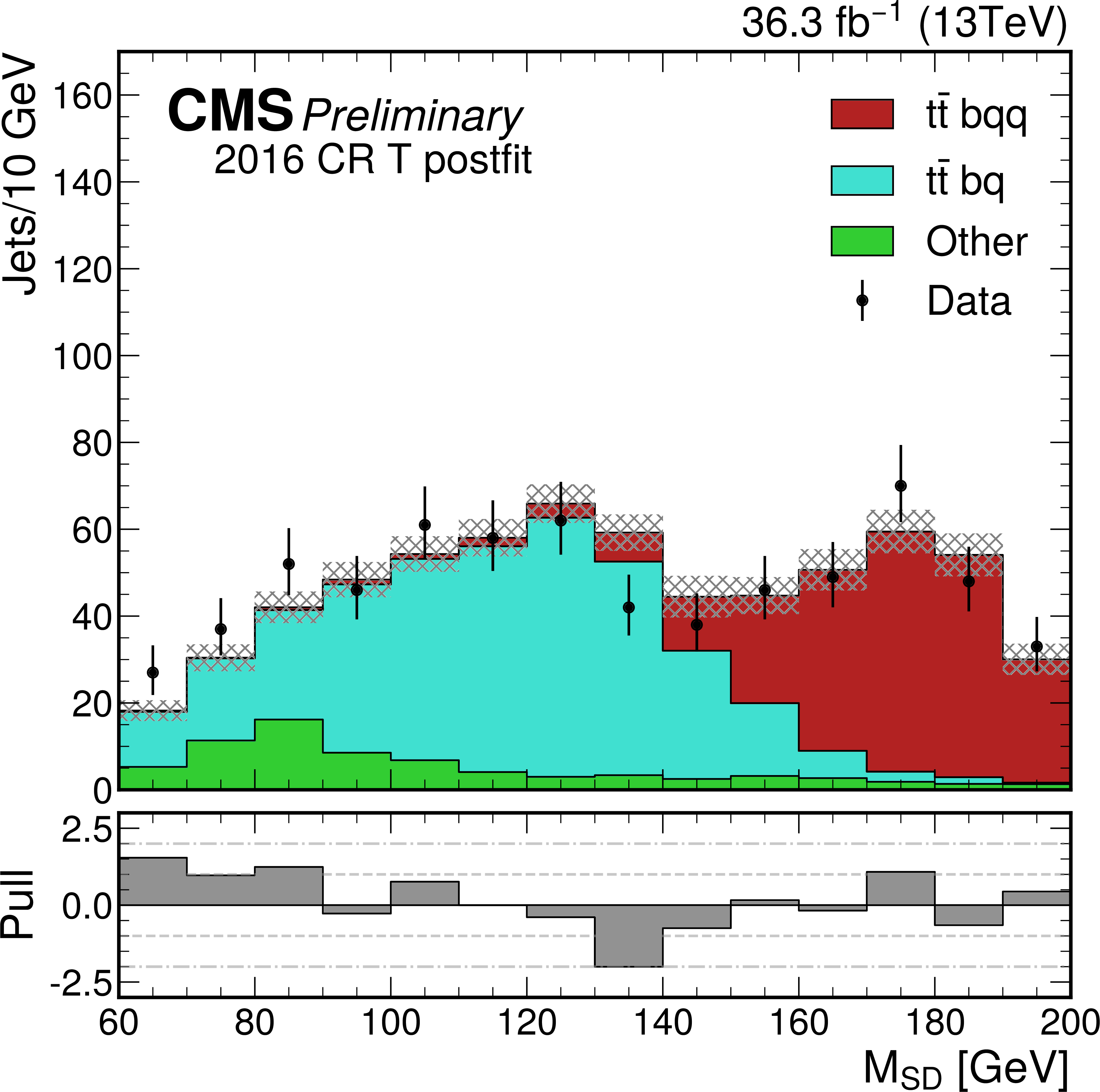
Additional Figure 27:
The softdrop mass distribution of the top-quark candidate jets in the 2016 semileptonic control region, tight ParticleNet category (CR T), after the joint semileptonic and hadronic signal region fit. Observed data (black markers) and the postfit estimate (filled histograms) are shown for the three jet categories. |
png pdf |
Additional Figure 28:
The softdrop mass distribution of the top-quark candidate jets in the 2017 semileptonic control region, loose ParticleNet category (CR L), after the joint semileptonic and hadronic signal region fit. Observed data (black markers) and the postfit estimate (filled histograms) are shown for the three jet categories. |
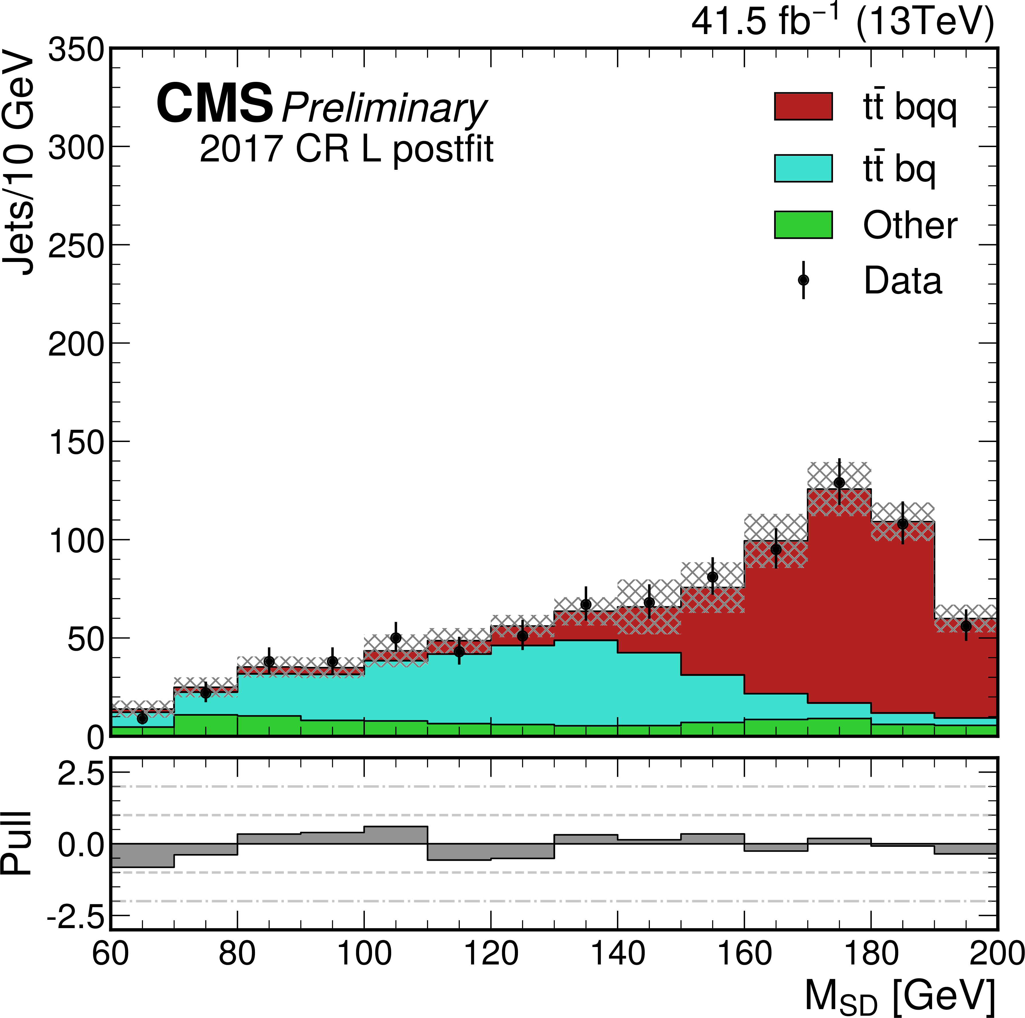
png pdf |
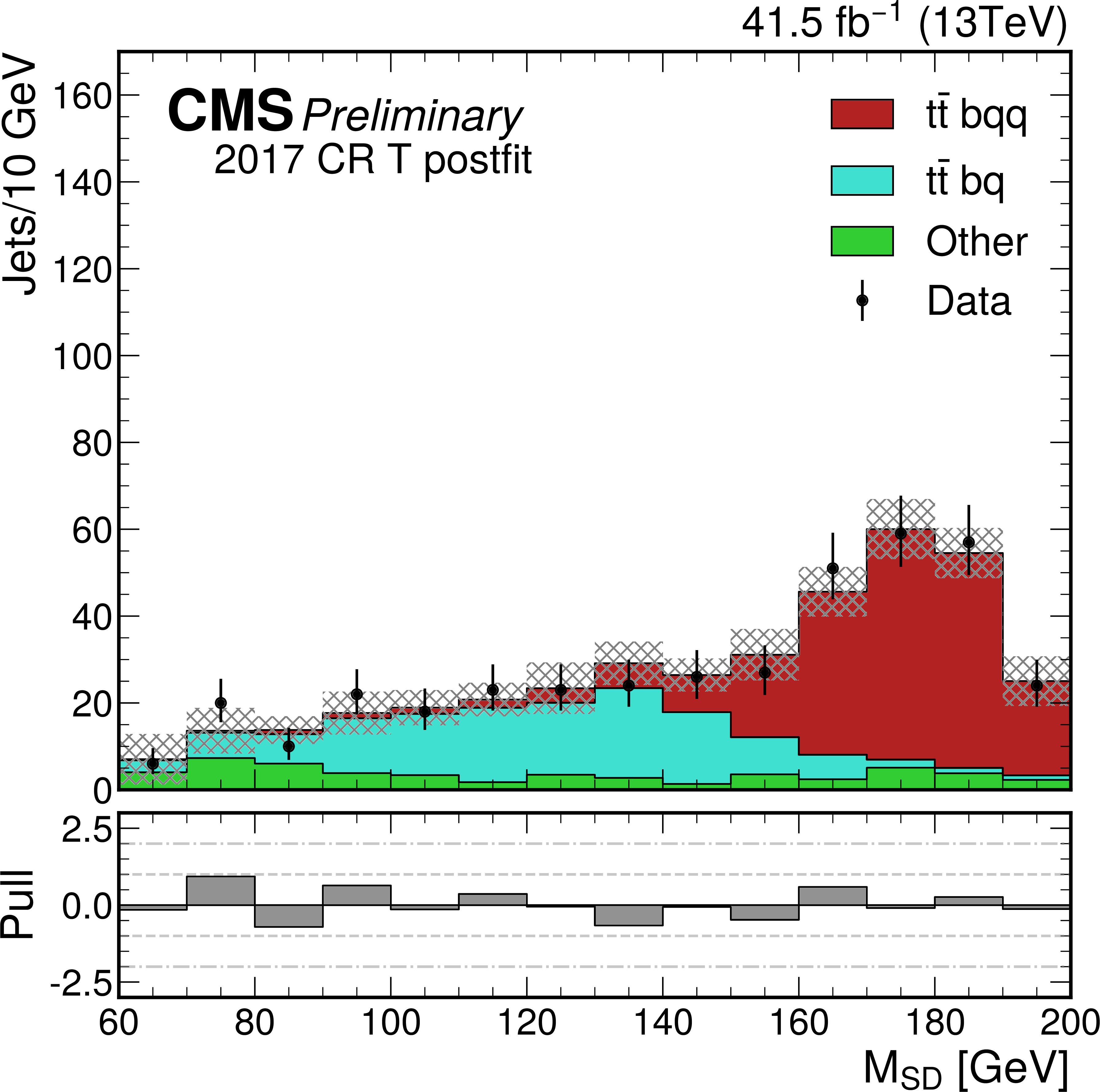
Additional Figure 29:
The softdrop mass distribution of the top-quark candidate jets in the 2017 semileptonic control region, tight ParticleNet category (CR T), after the joint semileptonic and hadronic signal region fit. Observed data (black markers) and the postfit estimate (filled histograms) are shown for the three jet categories. |
png pdf |
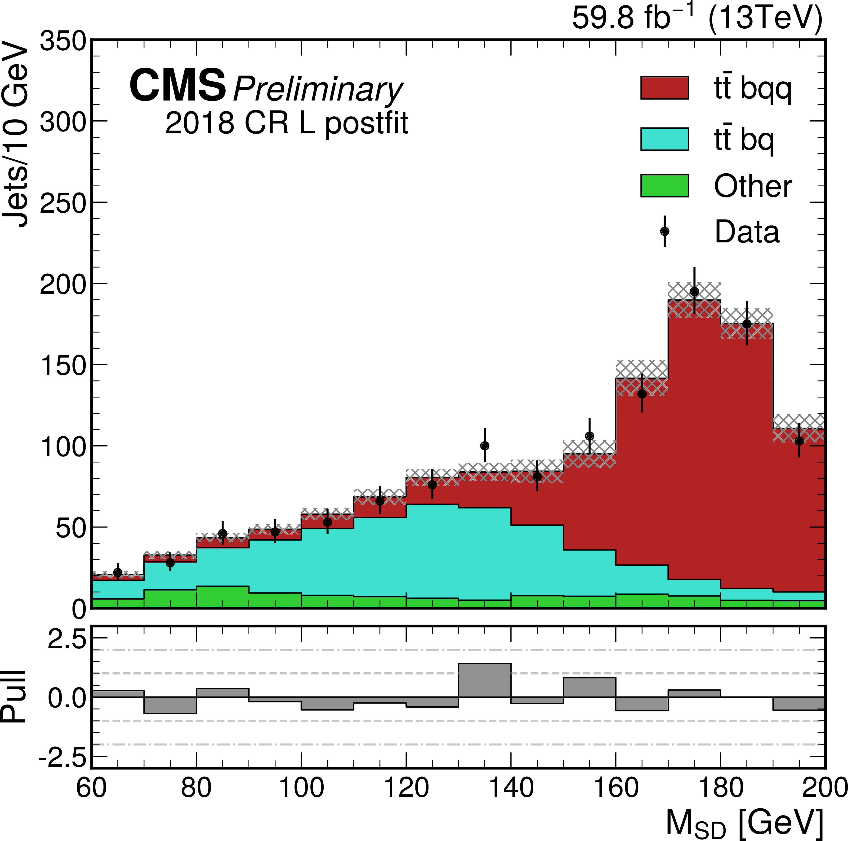
Additional Figure 30:
The softdrop mass distribution of the top-quark candidate jets in the 2018 semileptonic control region, loose ParticleNet category (CR L), after the joint semileptonic and hadronic signal region fit. Observed data (black markers) and the postfit estimate (filled histograms) are shown for the three jet categories. |
png pdf |
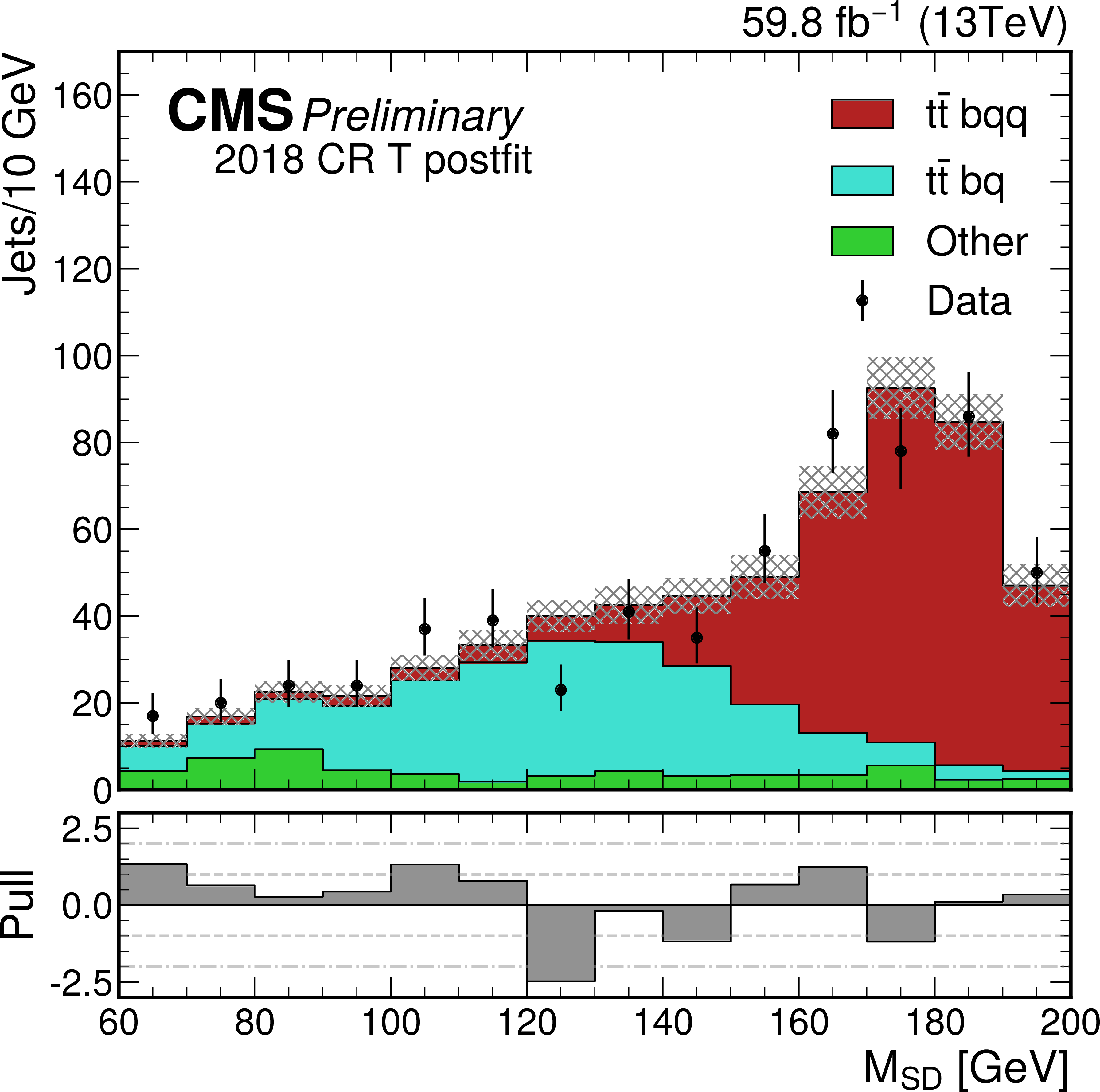
Additional Figure 31:
The softdrop mass distribution of the top-quark candidate jets in the 2018 semileptonic control region, tight ParticleNet category (CR T), after the joint semileptonic and hadronic signal region fit. Observed data (black markers) and the postfit estimate (filled histograms) are shown for the three jet categories. |
png pdf |
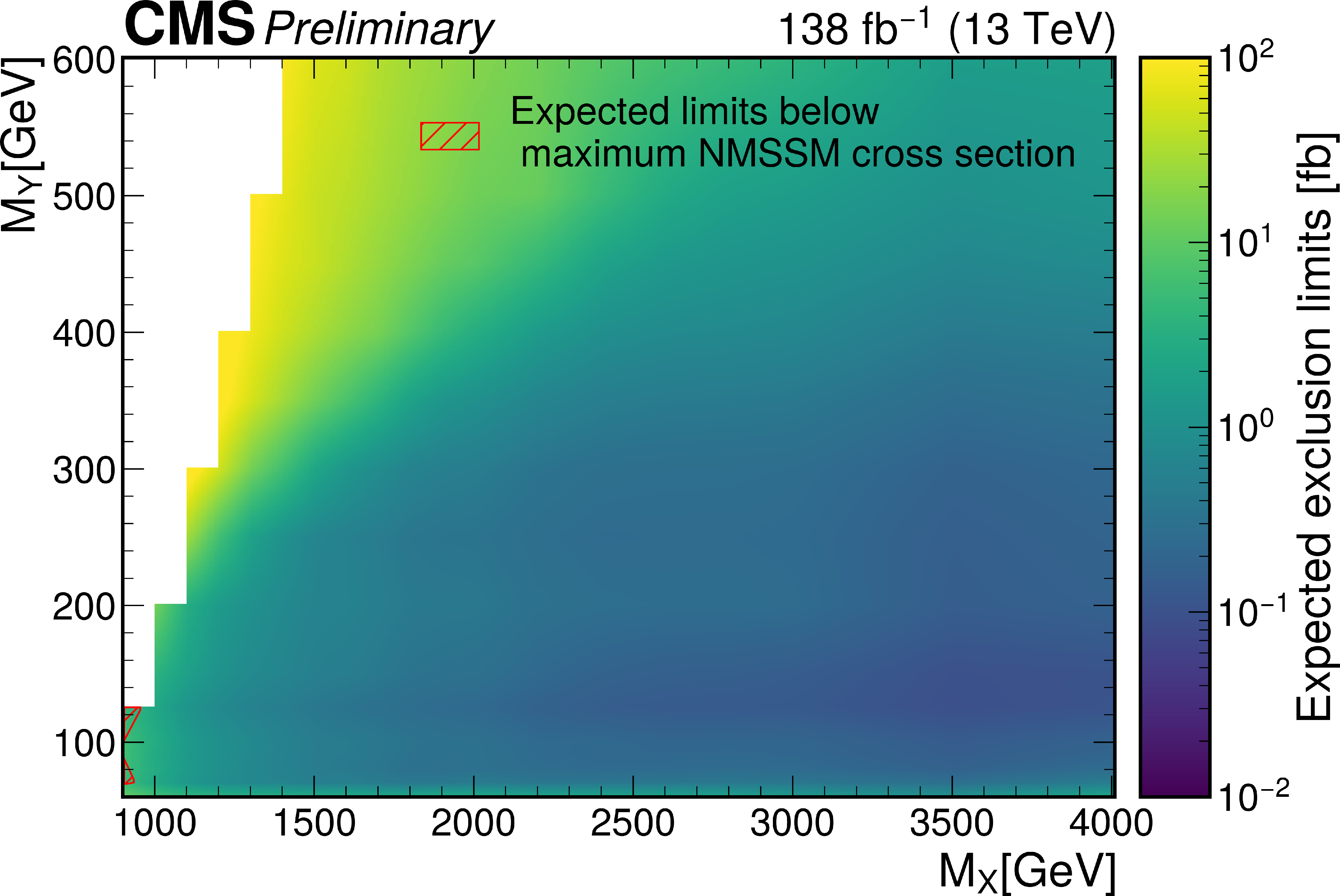
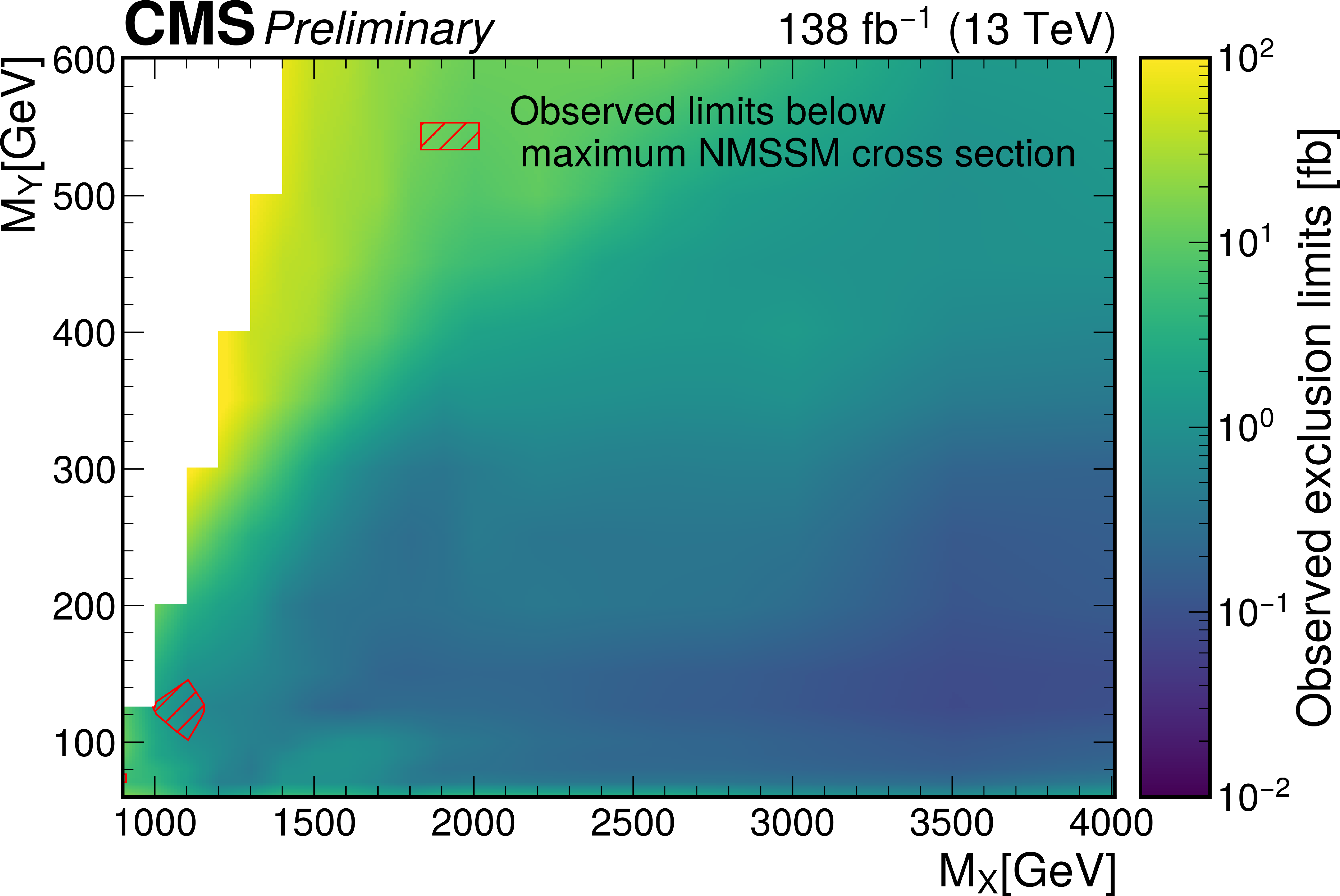
Additional Figure 32:
The 95% confidence level expected and observed limits on the signal cross-section as a function of $M_{\mathrm{X}}$ for different values of $M_{\mathrm{Y}}$. The red curves show the maximal possible cross sections of this process in NMSSM, taking into account all other theoretical and experimental constraints |
| References | ||||
| 1 | ATLAS Collaboration | Observation of a new particle in the search for the standard model Higgs boson with the ATLAS detector at the LHC | PLB 716 (2012) 01 | 1207.7214 |
| 2 | CMS Collaboration | Observation of a new boson at a mass of 125 GeV with the CMS experiment at the LHC | PLB 716 (2012) 30 | CMS-HIG-12-028 1207.7235 |
| 3 | CMS Collaboration | Observation of a new boson with mass near 125 GeV in pp collisions at $ \sqrt{s} = $ 7 and 8 TeV | JHEP 06 (2013) 081 | CMS-HIG-12-036 1303.4571 |
| 4 | P. W. Higgs | Broken symmetries, massless particles and gauge fields | PL12 (1964) 132 | |
| 5 | P. W. Higgs | Broken Symmetries and the Masses of Gauge Bosons | PRL 13 (1964) 508 | |
| 6 | G. S. Guralnik, C. R. Hagen, and T. W. B. Kibble | Global Conservation Laws and Massless Particles | PRL 13 (1964) 585 | |
| 7 | F. Englert and R. Brout | Broken Symmetry and the Mass of Gauge Vector Mesons | PRL 13 (1964) 321 | |
| 8 | P. W. Higgs | Spontaneous Symmetry Breakdown without Massless Bosons | PR145 (1966) 1156 | |
| 9 | T. W. B. Kibble | Symmetry breaking in nonAbelian gauge theories | PR155 (1967) 1554 | |
| 10 | D. Buttazzo et al. | Investigating the near-criticality of the Higgs boson | JHEP 12 (2013) 089 | 1307.3536 |
| 11 | Y. Hamada, H. Kawai, and K.-y. Oda | Bare Higgs mass at Planck scale | PRD 87 (2013), no. 5, 053009 | 1210.2538 |
| 12 | D. R. T. Jones | Comment on "Bare Higgs mass at Planck scale" | PRD 88 (2013), no. 9, 098301 | 1309.7335 |
| 13 | A. V. Bednyakov, B. A. Kniehl, A. F. Pikelner, and O. L. Veretin | Stability of the Electroweak Vacuum: Gauge Independence and Advanced Precision | PRL 115 (2015), no. 20, 201802 | 1507.08833 |
| 14 | J. Wess and B. Zumino | Supergauge Transformations in Four-Dimensions | NPB 70 (1974) 390 | |
| 15 | L. Randall and R. Sundrum | A large mass hierarchy from a small extra dimension | PRL 83 (1999) 3370 | hep-ph/9905221 |
| 16 | P. Fayet | Supergauge Invariant Extension of the Higgs Mechanism and a Model for the electron and Its Neutrino | NPB 90 (1975) 104 | |
| 17 | P. Fayet | Spontaneously Broken Supersymmetric Theories of Weak, Electromagnetic and Strong Interactions | PLB 69 (1977) 489 | |
| 18 | U. Ellwanger, C. Hugonie, and A. M. Teixeira | The Next-to-Minimal Supersymmetric Standard Model | PR 496 (2010) 1 | 0910.1785 |
| 19 | M. Maniatis | The Next-to-Minimal Supersymmetric extension of the Standard Model reviewed | Int. J. Mod. Phys. A 25 (2010) 3505 | 0906.0777 |
| 20 | J. E. Kim and H. P. Nilles | The mu Problem and the Strong CP Problem | PLB 138 (1984) 150 | |
| 21 | ATLAS Collaboration | Search for heavy Higgs bosons decaying into two tau leptons with the ATLAS detector using $ pp $ collisions at $ \sqrt{s}= $ 13 TeV | PRL 125 (2020), no. 5, 051801 | 2002.12223 |
| 22 | CMS Collaboration | Search for additional neutral MSSM Higgs bosons in the $ \tau\tau $ final state in proton-proton collisions at $ \sqrt{s}= $ 13 TeV | JHEP 09 (2018) 007 | CMS-HIG-17-020 1803.06553 |
| 23 | ATLAS Collaboration | Search for charged Higgs bosons decaying via $ H^{\pm} \to \tau^{\pm}\nu_{\tau} $ in the $ \tau $+jets and $ \tau $+lepton final states with 36 fb$ ^{-1} $ of $ pp $ collision data recorded at $ \sqrt{s} = $ 13 TeV with the ATLAS experiment | JHEP 09 (2018) 139 | 1807.07915 |
| 24 | CMS Collaboration | Search for charged Higgs bosons in the H$ ^{\pm} \to \tau^{\pm}\nu_\tau $ decay channel in proton-proton collisions at $ \sqrt{s} = $ 13 TeV | JHEP 07 (2019) 142 | CMS-HIG-18-014 1903.04560 |
| 25 | U. Ellwanger and M. Rodriguez-Vazquez | Simultaneous search for extra light and heavy Higgs bosons via cascade decays | JHEP 11 (2017) 008 | 1707.08522 |
| 26 | CMS Collaboration | Search for a heavy Higgs boson decaying into two lighter Higgs bosons in the $ \tau\tau $bb final state at 13 TeV | 2021. Submitted to JHEP | CMS-HIG-20-014 2106.10361 |
| 27 | T. Robens, T. Stefaniak, and J. Wittbrodt | Two-real-scalar-singlet extension of the SM: LHC phenomenology and benchmark scenarios | EPJC 80 (2020) 151 | 1908.08554 |
| 28 | CMS Collaboration | Precision luminosity measurement in proton-proton collisions at $ \sqrt{s} = $ 13 TeV in 2015 and 2016 at CMS | EPJC 81 (Apr, 2021) 800 | CMS-LUM-17-003 2104.01927 |
| 29 | CMS Collaboration | The CMS experiment at the CERN LHC | JINST 3 (2008) S08004 | CMS-00-001 |
| 30 | CMS Collaboration | Performance of the CMS Level-1 trigger in proton-proton collisions at $ \sqrt{s} = $ 13 TeV | JINST 15 (2020) P10017 | CMS-TRG-17-001 2006.10165 |
| 31 | CMS Collaboration | The CMS trigger system | JINST 12 (2017) P01020 | CMS-TRG-12-001 1609.02366 |
| 32 | M. Cacciari, G. P. Salam, and G. Soyez | The anti-$ k_t $ jet clustering algorithm | JHEP 04 (2008) 063 | 0802.1189 |
| 33 | M. Cacciari, G. P. Salam, and G. Soyez | FastJet user manual | EPJC 72 (2012) 1896 | 1111.6097 |
| 34 | CMS Collaboration | Particle-flow reconstruction and global event description with the CMS detector | JINST 12 (2017) P10003 | CMS-PRF-14-001 1706.04965 |
| 35 | CMS Collaboration | Pileup mitigation at CMS in 13 TeV data | JINST 15 (2020) P09018 | CMS-JME-18-001 2003.00503 |
| 36 | CMS Collaboration | Performance of missing transverse momentum reconstruction in proton-proton collisions at $ \sqrt{s} = $ 13 TeV using the CMS detector | JINST 14 (2019) P07004 | CMS-JME-17-001 1903.06078 |
| 37 | J. Alwall et al. | The automated computation of tree-level and next-to-leading order differential cross sections, and their matching to parton shower simulations | JHEP 07 (2014) 079 | 1405.0301 |
| 38 | NNPDF Collaboration | Parton distributions for the lhc run ii | JHEP 04 (2015) 040 | 1410.8849 |
| 39 | A. Buckley et al. | LHAPDF6: parton density access in the LHC precision era | EPJC 75 (2015) 132 | 1412.7420 |
| 40 | T. Sjostrand et al. | An Introduction to PYTHIA 8.2 | CPC 191 (2015) 159 | 1410.3012 |
| 41 | S. Frixione, G. Ridolfi, and P. Nason | A positive-weight next-to-leading-order Monte Carlo for heavy flavour hadroproduction | JHEP 09 (2007) 126 | 0707.3088 |
| 42 | S. Frixione, P. Nason, and C. Oleari | Matching NLO QCD computations with parton shower simulations: the POWHEG method | JHEP 11 (2007) 070 | 0709.2092 |
| 43 | S. Alioli, P. Nason, C. Oleari, and E. Re | A general framework for implementing NLO calculations in shower Monte Carlo programs: the POWHEG BOX | JHEP 06 (2010) 043 | 1002.2581 |
| 44 | M. Czakon and A. Mitov | Top++: A program for the calculation of the top-pair cross-section at hadron colliders | CPC 185 (2014) 2930 | 1112.5675 |
| 45 | J. Allison et al. | Geant4 developments and applications | IEEE Trans. Nucl. Sci. 53 (2006) 270 | |
| 46 | CMS Collaboration | Measurement of the inelastic proton-proton cross section at $ \sqrt{s} = $ 13 TeV | JHEP 07 (2018) 161 | CMS-FSQ-15-005 1802.02613 |
| 47 | D. Krohn, J. Thaler, and L.-T. Wang | Jet trimming | JHEP 02 (2010) 084 | 0912.1342 |
| 48 | CMS Collaboration | Identification of heavy-flavour jets with the CMS detector in pp collisions at 13 TeV | JINST 13 (2018) P05011 | CMS-BTV-16-002 1712.07158 |
| 49 | M. Dasgupta, A. Fregoso, S. Marzani, and G. P. Salam | Towards an understanding of jet substructure | JHEP 09 (2013) 029 | 1307.0007 |
| 50 | A. J. Larkoski, S. Marzani, G. Soyez, and J. Thaler | Soft drop | JHEP 05 (2014) 146 | 1402.2657 |
| 51 | D. Bertolini, P. Harris, M. Low, and N. Tran | Pileup per particle identification | JHEP 10 (2014) 059 | 1407.6013 |
| 52 | H. Qu and L. Gouskos | ParticleNet: Jet Tagging via Particle Clouds | PRD 101 (2020), no. 5, 056019 | 1902.08570 |
| 53 | CMS Collaboration | Identification of highly Lorentz-boosted heavy particles using graph neural networks and new mass decorrelation techniques | CDS | |
| 54 | CMS Collaboration | Search for resonant Higgs boson pair production in four b quark final state using large-area jets in proton-proton collisions at $ \sqrt{s}= $ 13 TeV | CMS-PAS-B2G-20-004 | CMS-PAS-B2G-20-004 |
| 55 | CMS Collaboration | Identification of heavy, energetic, hadronically decaying particles using machine-learning techniques | JINST 15 (2020), no. 06, P06005 | CMS-JME-18-002 2004.08262 |
| 56 | E. Bols et al. | Jet Flavour Classification Using DeepJet | JINST 15 (2020) P12012 | 2008.10519 |
| 57 | R. G. Lomax and D. L. Hahs-Vaughn | Statistical concepts: a second course | Taylor and Francis, Hoboken, NJ | |
| 58 | CMS Collaboration | Measurement of the top quark mass with lepton+jets final states using $ {\mathrm{p}}{\mathrm{p}} $ collisions at $ \sqrt{s} = $ 13 TeV | EPJC 78 (2018) 891 | CMS-TOP-17-007 1805.01428 |
| 59 | J. Butterworth et al. | PDF4LHC recommendations for LHC Run II | JPG 43 (2016) 023001 | 1510.03865 |
| 60 | R. Barlow and C. Beeston | Fitting using finite Monte Carlo samples | CPC 77 (1993) 219 | |
| 61 | J. S. Conway | Incorporating nuisance parameters in likelihoods for multisource spectra | in Proceedings, PHYSTAT 2011 Workshop on Statistical Issues Related to Discovery Claims in Search Experiments and Unfolding, CERN, 2011 | 1103.0354 |
| 62 | A. L. Read | Presentation of search results: the CL$ _s $ technique | JPG 28 (2002) 2693 | |
| 63 | T. Junk | Confidence level computation for combining searches with small statistics | NIMA 434 (1999) 435 | hep-ex/9902006 |
|
|
Compact Muon Solenoid LHC, CERN |
|

|

|

|

|

|