

Compact Muon Solenoid
LHC, CERN
| CMS-PAS-B2G-20-013 | ||
| Search for heavy resonances and nonresonant axion-like particles in semileptonic ZZ, ZW, or ZH final states at $\sqrt{s}= $ 13 TeV | ||
| CMS Collaboration | ||
| July 2021 | ||
| Abstract: A search has been performed for heavy resonances and nonresonant axion-like particles (ALPs) in semileptonic ZZ, ZW, or ZH final states, with two charged leptons (electrons or muons) produced by the decay of a Z boson, and two quarks produced by the decay of a Z, W, or H boson. The analysis is sensitive to resonances with masses in the range from 450 to 1800 GeV decaying into ZZ or ZW. A search for the effects of nonresonant ALP-mediated ZZ or ZH production is included. Two categories are defined based on the merged or resolved reconstruction of the hadronically decaying boson. The search is based on data collected during 2016 to 2018 by the CMS experiment at the LHC in proton-proton collisions with a center-of-mass energy of 13 TeV, corresponding to an integrated luminosity of 137 fb$^{-1}$. No excess is observed in the data above the standard model background expectation. Upper limits on the production cross section of heavy, narrow spin-1 and spin-2 resonances are derived as a function of the resonance mass, and exclusion limits on the production of W' bosons and bulk graviton particles are calculated in the framework of the heavy vector triplet model and warped extra dimensions, respectively. In addition, upper limits on the ALP-mediated diboson production cross section and ALP couplings to standard model particles are obtained in the framework of linear and chiral effective field theories. | ||
|
Links:
CDS record (PDF) ;
CADI line (restricted) ;
These preliminary results are superseded in this paper, Submitted to JHEP. The superseded preliminary plots can be found here. |
||
| Figures | |
png pdf |
Figure 1:
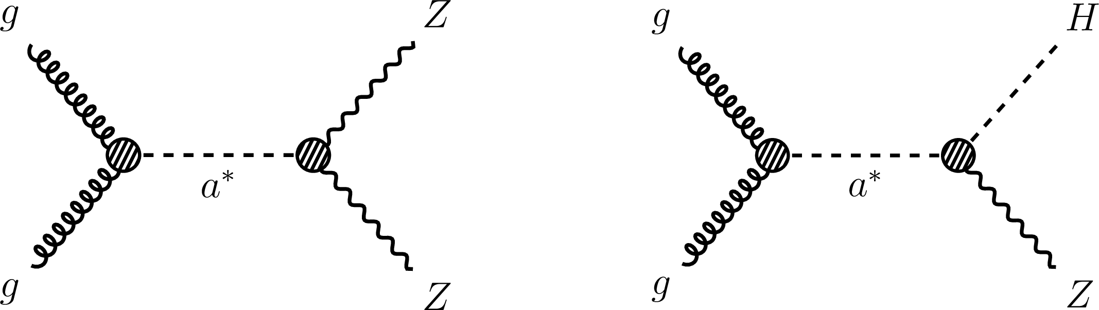
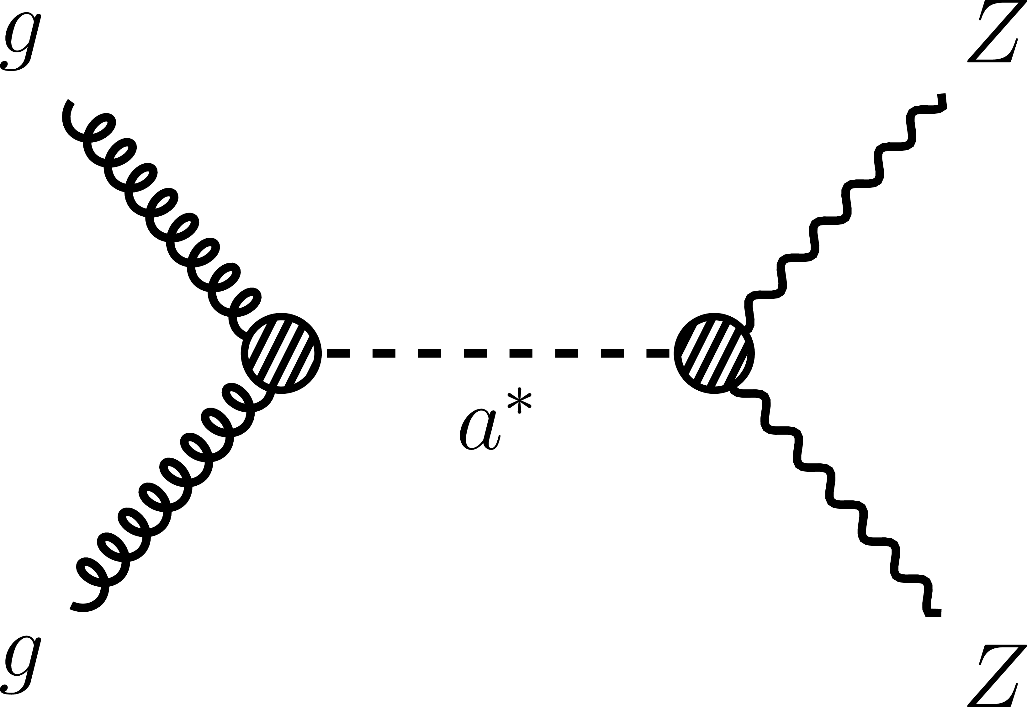
Feynman diagrams for the processes $\mathrm{g} \mathrm{g} \to \mathrm{Z} \mathrm{Z} $ (left) and $\mathrm{g} \mathrm{g} \to \mathrm{Z} \mathrm{H} $ (right) via an off-shell ALP a* in the $s$ channel. |
png pdf |
Figure 1-a:
Feynman diagrams for the processes $\mathrm{g} \mathrm{g} \to \mathrm{Z} \mathrm{Z} $ (left) and $\mathrm{g} \mathrm{g} \to \mathrm{Z} \mathrm{H} $ (right) via an off-shell ALP a* in the $s$ channel. |

png pdf |
Figure 1-b:
Feynman diagrams for the processes $\mathrm{g} \mathrm{g} \to \mathrm{Z} \mathrm{Z} $ (left) and $\mathrm{g} \mathrm{g} \to \mathrm{Z} \mathrm{H} $ (right) via an off-shell ALP a* in the $s$ channel. |
png pdf |
Figure 2:
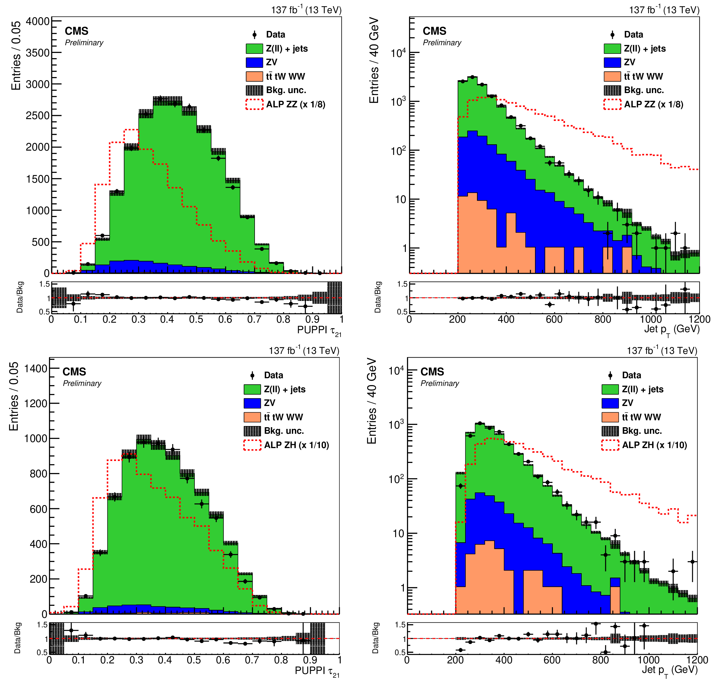
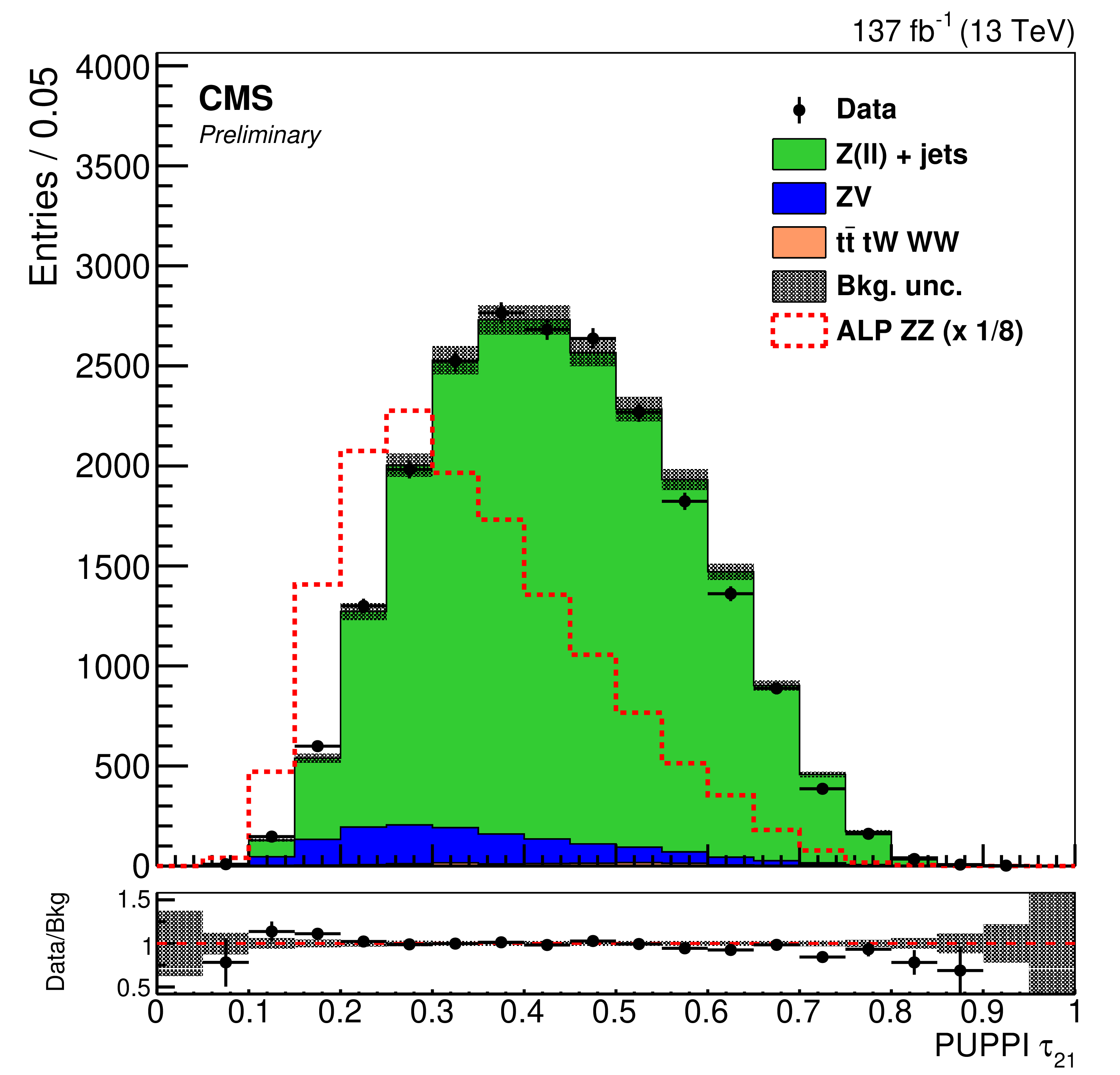
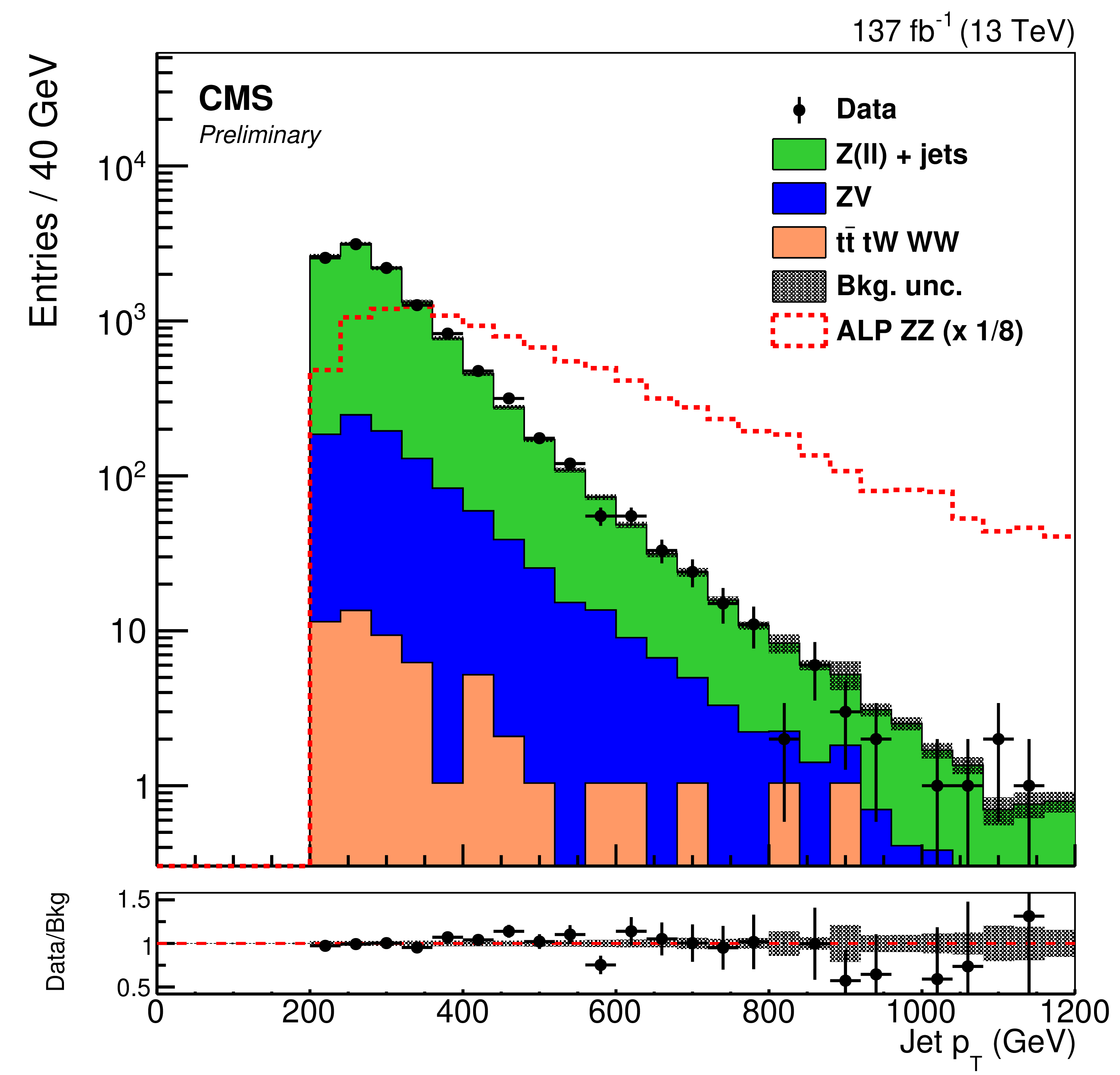
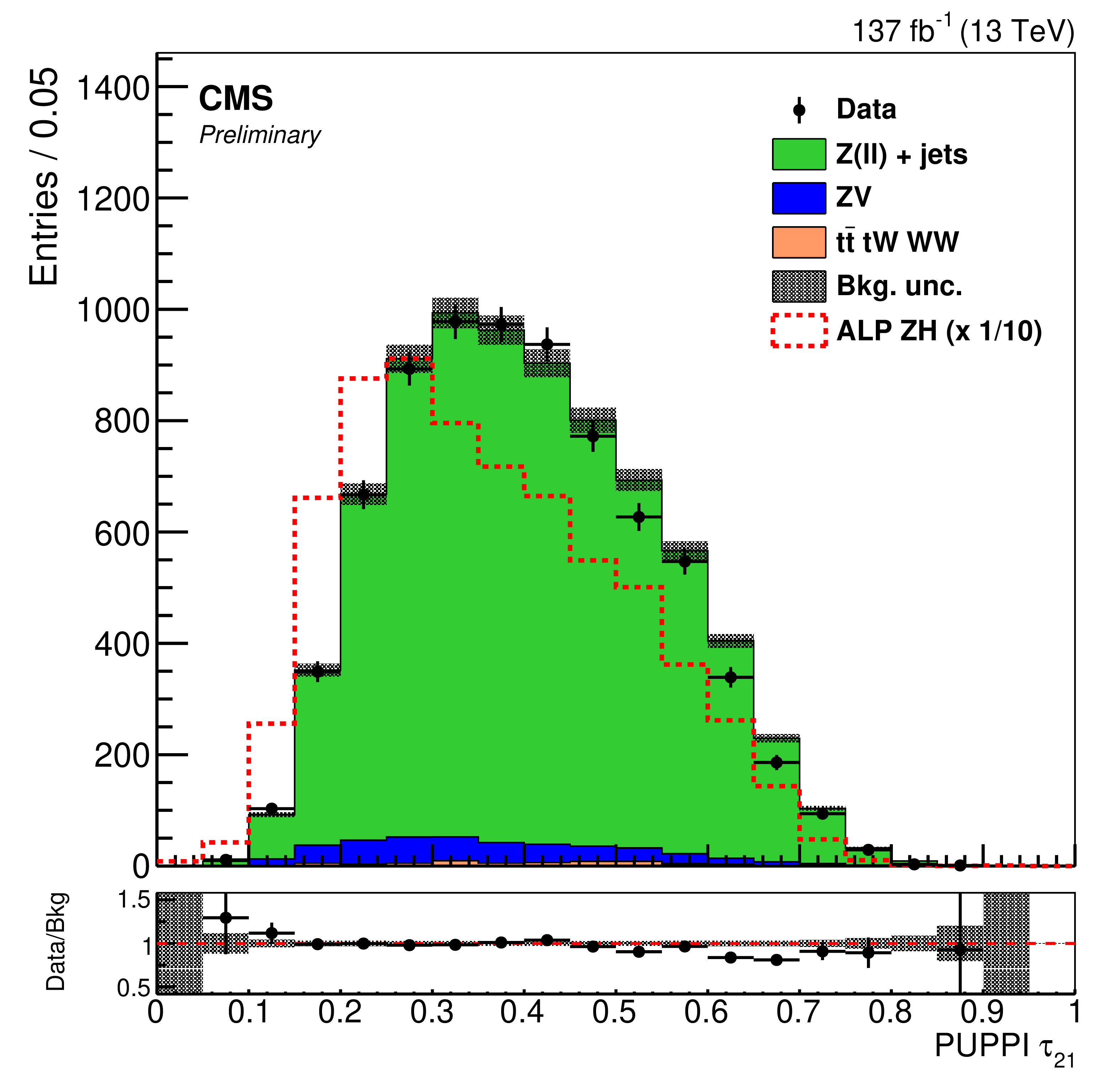
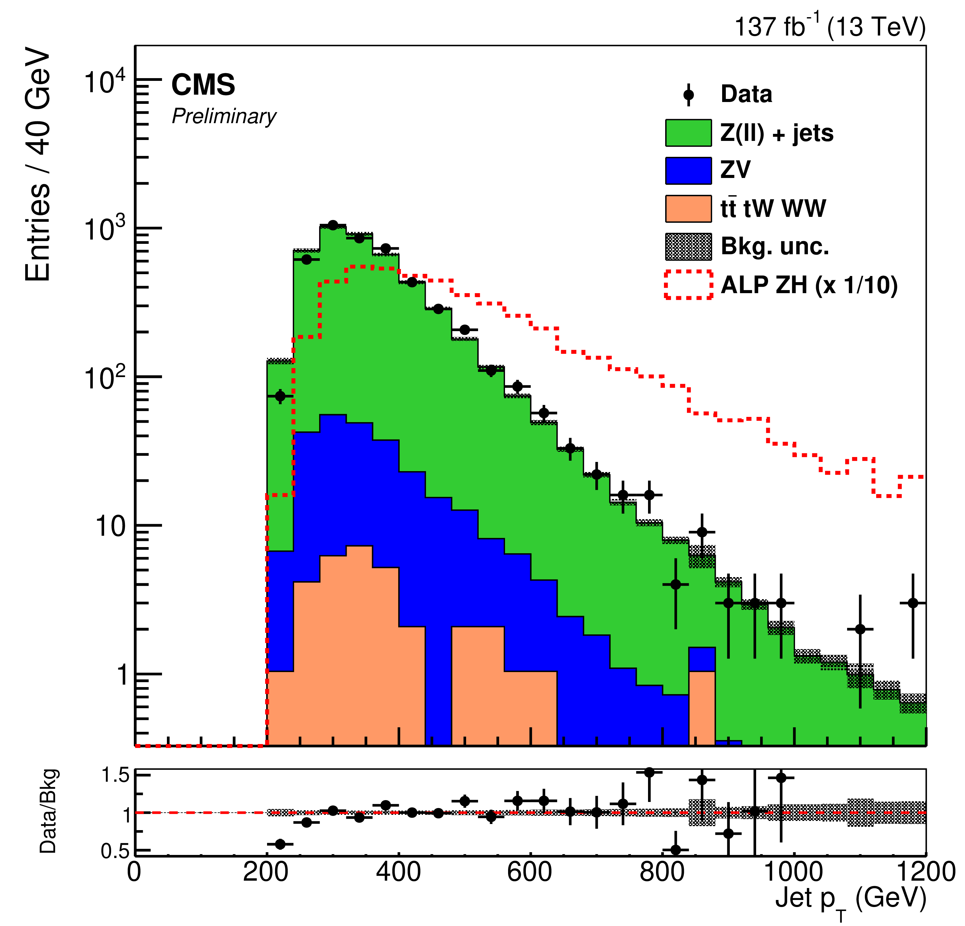
Distributions of ${\tau _{21}}$ and ${p_{\mathrm {T}}}$ (${{\mathrm {J}}}$) (after applying the ${\tau _{21}}$ selection) for boosted hadronic V (top) and H candidates (bottom). The gray band shows the statistical and systematic uncertainties on the background. The background for the ${\tau _{21}}$ distributions is normalized to the number of events in the data; the background normalization for the ${p_{\mathrm {T}}}$ (${{\mathrm {J}}}$) distributions is derived from the final fit to the data. The red dashed histograms correspond to a hypothetical linear (chiral) ALP with 1 TeV$ ^{-1}$ couplings to gluons and $\mathrm{Z} \mathrm{Z} $ (ZH), and $f_{\mathrm{a}} = $ 3 TeV; the cross sections have been scaled, as shown in the legend, for better visibility. The lower panel shows the ratio of data to background. |
png pdf |
Figure 2-a:
Distributions of ${\tau _{21}}$ and ${p_{\mathrm {T}}}$ (${{\mathrm {J}}}$) (after applying the ${\tau _{21}}$ selection) for boosted hadronic V (top) and H candidates (bottom). The gray band shows the statistical and systematic uncertainties on the background. The background for the ${\tau _{21}}$ distributions is normalized to the number of events in the data; the background normalization for the ${p_{\mathrm {T}}}$ (${{\mathrm {J}}}$) distributions is derived from the final fit to the data. The red dashed histograms correspond to a hypothetical linear (chiral) ALP with 1 TeV$ ^{-1}$ couplings to gluons and $\mathrm{Z} \mathrm{Z} $ (ZH), and $f_{\mathrm{a}} = $ 3 TeV; the cross sections have been scaled, as shown in the legend, for better visibility. The lower panel shows the ratio of data to background. |
png pdf |
Figure 2-b:
Distributions of ${\tau _{21}}$ and ${p_{\mathrm {T}}}$ (${{\mathrm {J}}}$) (after applying the ${\tau _{21}}$ selection) for boosted hadronic V (top) and H candidates (bottom). The gray band shows the statistical and systematic uncertainties on the background. The background for the ${\tau _{21}}$ distributions is normalized to the number of events in the data; the background normalization for the ${p_{\mathrm {T}}}$ (${{\mathrm {J}}}$) distributions is derived from the final fit to the data. The red dashed histograms correspond to a hypothetical linear (chiral) ALP with 1 TeV$ ^{-1}$ couplings to gluons and $\mathrm{Z} \mathrm{Z} $ (ZH), and $f_{\mathrm{a}} = $ 3 TeV; the cross sections have been scaled, as shown in the legend, for better visibility. The lower panel shows the ratio of data to background. |
png pdf |
Figure 2-c:
Distributions of ${\tau _{21}}$ and ${p_{\mathrm {T}}}$ (${{\mathrm {J}}}$) (after applying the ${\tau _{21}}$ selection) for boosted hadronic V (top) and H candidates (bottom). The gray band shows the statistical and systematic uncertainties on the background. The background for the ${\tau _{21}}$ distributions is normalized to the number of events in the data; the background normalization for the ${p_{\mathrm {T}}}$ (${{\mathrm {J}}}$) distributions is derived from the final fit to the data. The red dashed histograms correspond to a hypothetical linear (chiral) ALP with 1 TeV$ ^{-1}$ couplings to gluons and $\mathrm{Z} \mathrm{Z} $ (ZH), and $f_{\mathrm{a}} = $ 3 TeV; the cross sections have been scaled, as shown in the legend, for better visibility. The lower panel shows the ratio of data to background. |
png pdf |
Figure 2-d:
Distributions of ${\tau _{21}}$ and ${p_{\mathrm {T}}}$ (${{\mathrm {J}}}$) (after applying the ${\tau _{21}}$ selection) for boosted hadronic V (top) and H candidates (bottom). The gray band shows the statistical and systematic uncertainties on the background. The background for the ${\tau _{21}}$ distributions is normalized to the number of events in the data; the background normalization for the ${p_{\mathrm {T}}}$ (${{\mathrm {J}}}$) distributions is derived from the final fit to the data. The red dashed histograms correspond to a hypothetical linear (chiral) ALP with 1 TeV$ ^{-1}$ couplings to gluons and $\mathrm{Z} \mathrm{Z} $ (ZH), and $f_{\mathrm{a}} = $ 3 TeV; the cross sections have been scaled, as shown in the legend, for better visibility. The lower panel shows the ratio of data to background. |
png pdf |
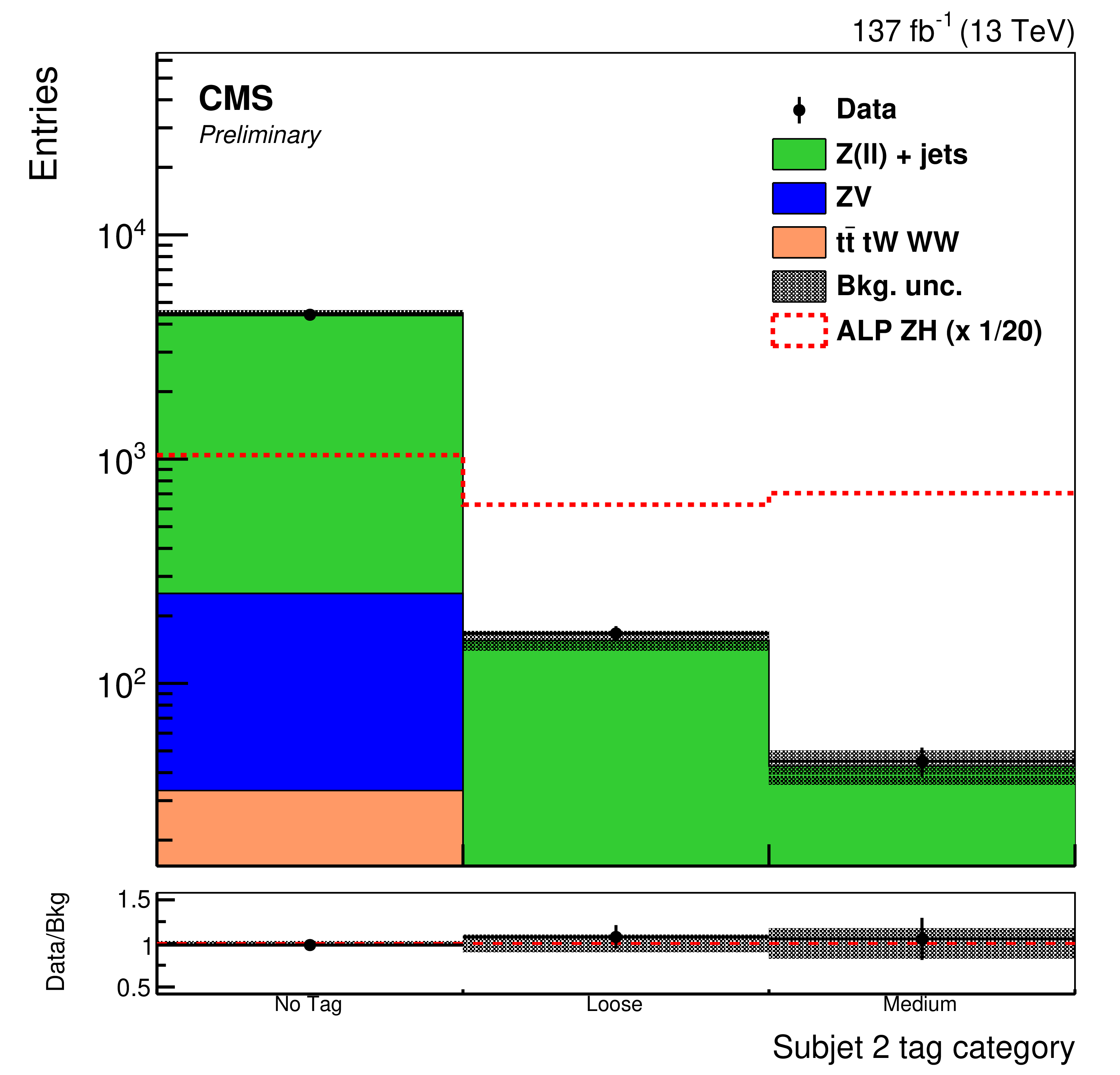
Figure 3:
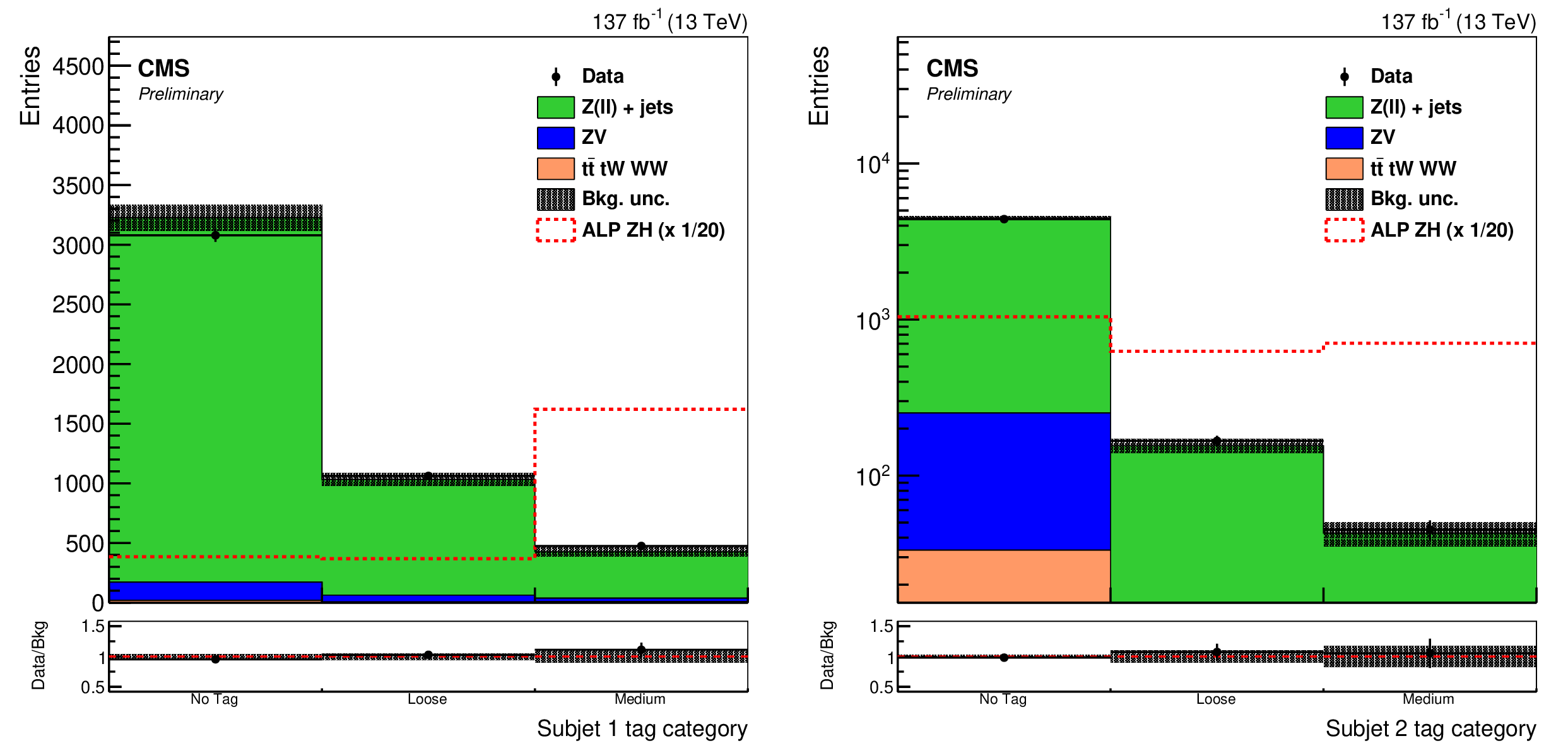
Distributions of the zero, loose, and medium DeepCSV tags for the most b-like subjet (left) and the less b-like subjet (right) of the boosted hadronic H candidates in SR2. The gray band shows the statistical and systematic uncertainties on the background. Background normalizations are derived from the final fit to the data. The red dashed histograms correspond to a hypothetical chiral ALP with $1 TeV ^{-1}$ couplings to gluons and ZH, and $f_a = $ 3 TeV; the cross section has been scaled, as shown in the legend, for better visibility. The lower panel shows the ratio of data to background. |

png pdf |
Figure 3-a:
Distributions of the zero, loose, and medium DeepCSV tags for the most b-like subjet (left) and the less b-like subjet (right) of the boosted hadronic H candidates in SR2. The gray band shows the statistical and systematic uncertainties on the background. Background normalizations are derived from the final fit to the data. The red dashed histograms correspond to a hypothetical chiral ALP with $1 TeV ^{-1}$ couplings to gluons and ZH, and $f_a = $ 3 TeV; the cross section has been scaled, as shown in the legend, for better visibility. The lower panel shows the ratio of data to background. |
png pdf |
Figure 3-b:
Distributions of the zero, loose, and medium DeepCSV tags for the most b-like subjet (left) and the less b-like subjet (right) of the boosted hadronic H candidates in SR2. The gray band shows the statistical and systematic uncertainties on the background. Background normalizations are derived from the final fit to the data. The red dashed histograms correspond to a hypothetical chiral ALP with $1 TeV ^{-1}$ couplings to gluons and ZH, and $f_a = $ 3 TeV; the cross section has been scaled, as shown in the legend, for better visibility. The lower panel shows the ratio of data to background. |

png pdf |
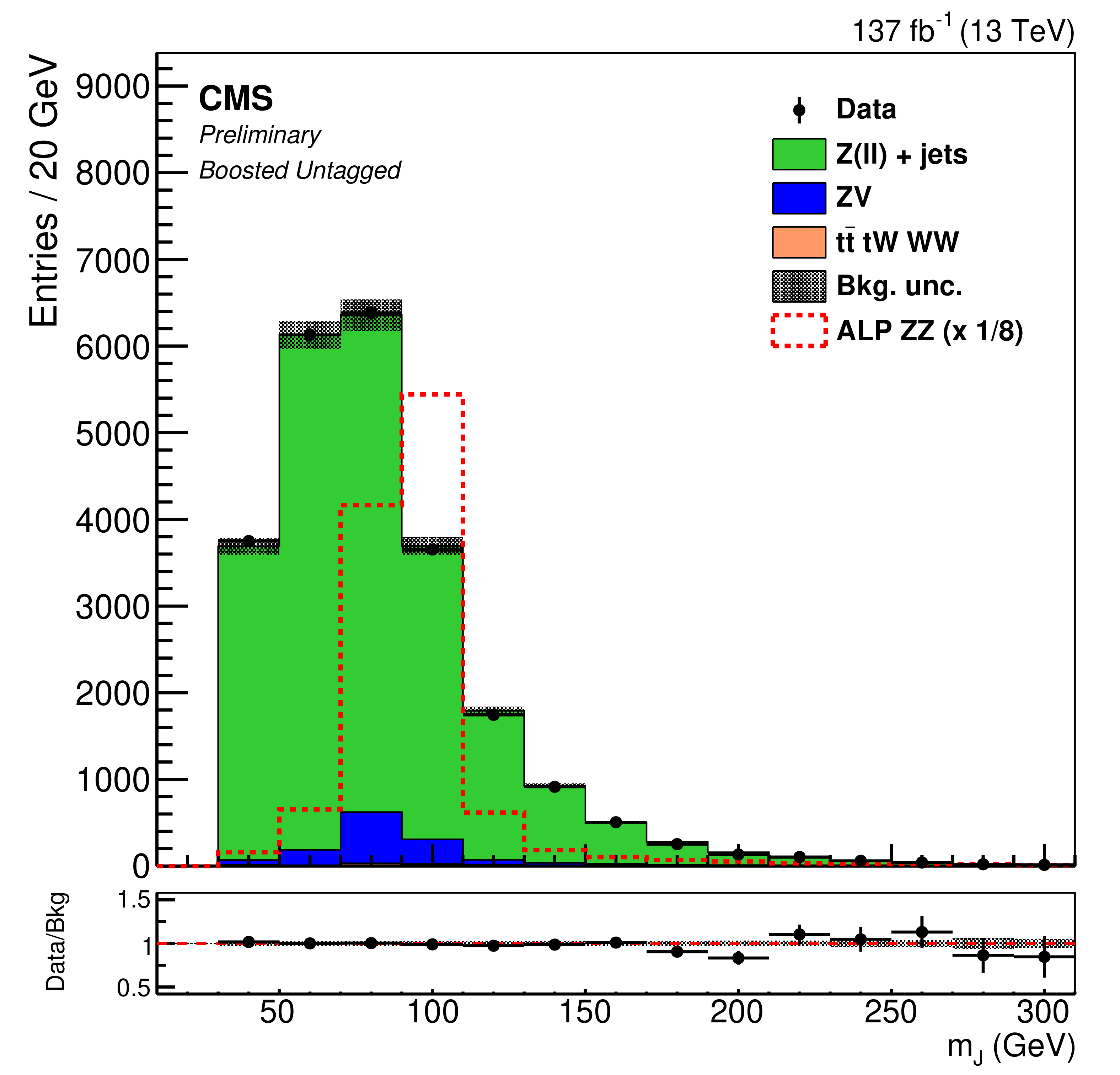
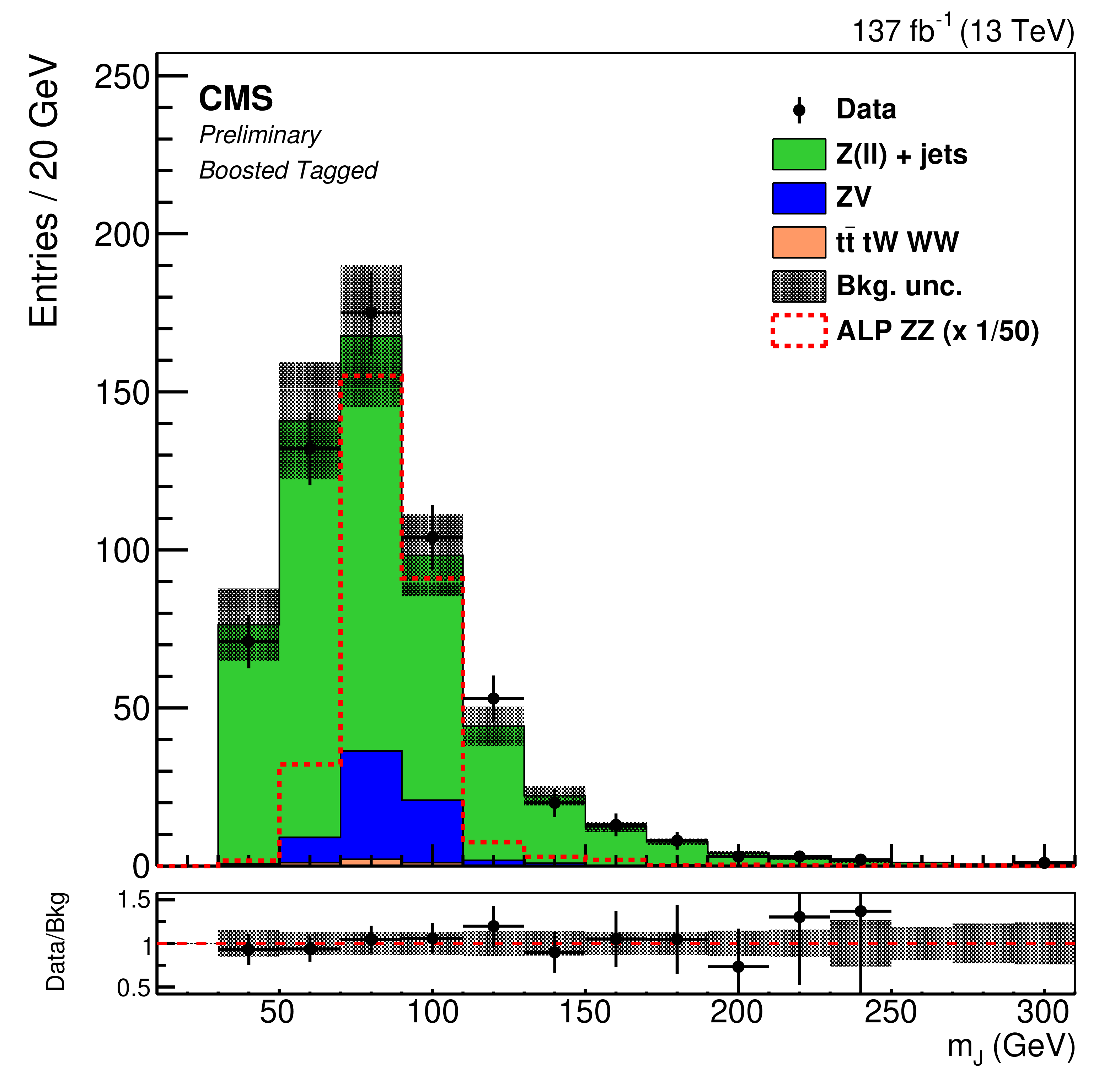
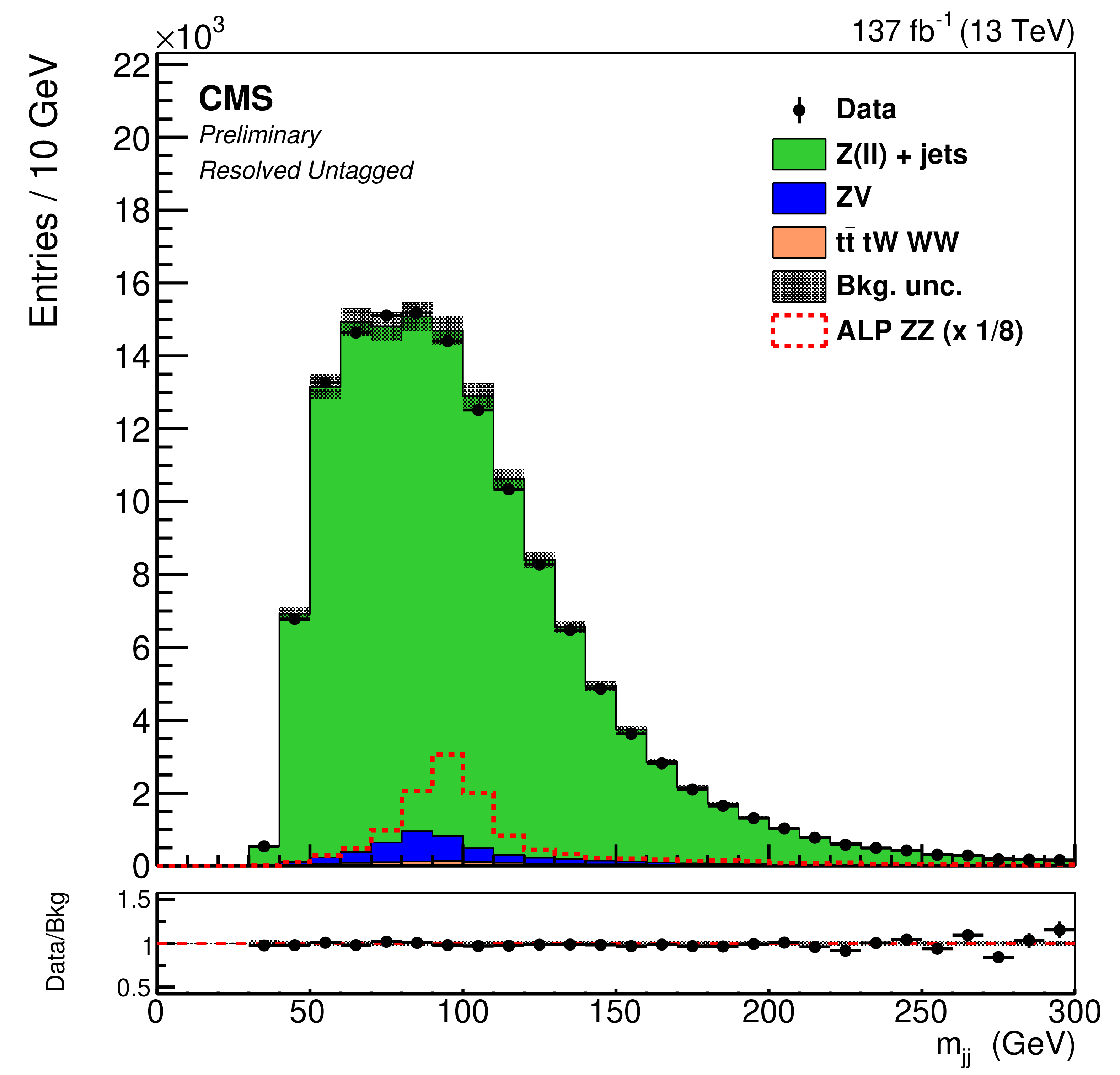
Figure 4:
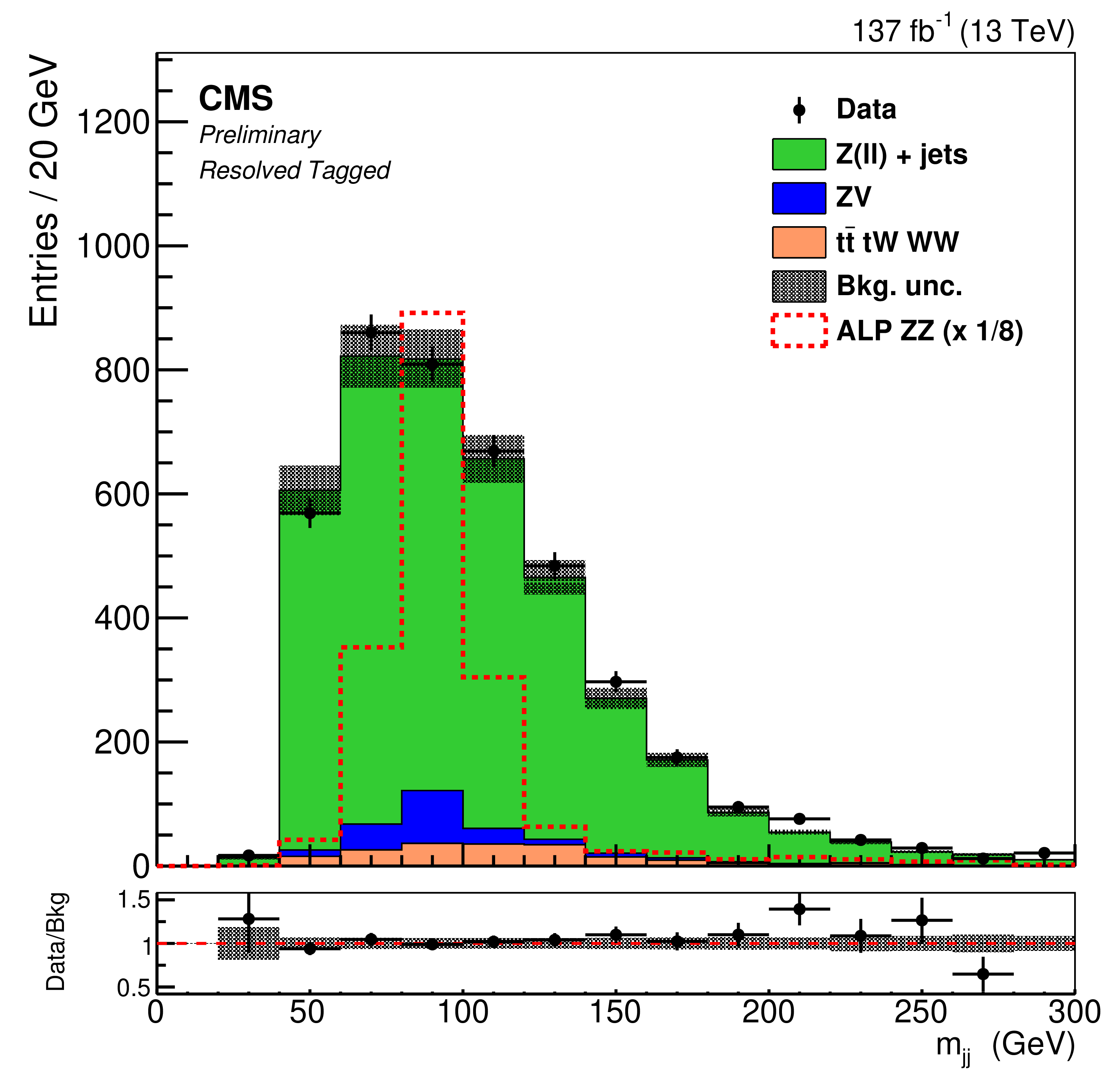
Distributions of the merged jet ${m_\mathrm {J}}$ (top) and the dijet ${m_\mathrm {jj}}$ (bottom) for the untagged (left) and tagged (right) categories. Signal regions SR1 and SR2 and sideband SB have been defined in the text. The gray band shows the statistical and systematic uncertainties on the background. Background normalizations are derived from the final fit to the data. The red dashed histograms correspond to a hypothetical linear ALP with $1 TeV ^{-1}$ couplings to gluons and ZZ, and $f_a = $ 3 TeV; the cross section has been scaled, as shown in the legend, for better visibility. The lower panel shows the ratio of data to background. |
png pdf |
Figure 4-a:
Distributions of the merged jet ${m_\mathrm {J}}$ (top) and the dijet ${m_\mathrm {jj}}$ (bottom) for the untagged (left) and tagged (right) categories. Signal regions SR1 and SR2 and sideband SB have been defined in the text. The gray band shows the statistical and systematic uncertainties on the background. Background normalizations are derived from the final fit to the data. The red dashed histograms correspond to a hypothetical linear ALP with $1 TeV ^{-1}$ couplings to gluons and ZZ, and $f_a = $ 3 TeV; the cross section has been scaled, as shown in the legend, for better visibility. The lower panel shows the ratio of data to background. |
png pdf |
Figure 4-b:
Distributions of the merged jet ${m_\mathrm {J}}$ (top) and the dijet ${m_\mathrm {jj}}$ (bottom) for the untagged (left) and tagged (right) categories. Signal regions SR1 and SR2 and sideband SB have been defined in the text. The gray band shows the statistical and systematic uncertainties on the background. Background normalizations are derived from the final fit to the data. The red dashed histograms correspond to a hypothetical linear ALP with $1 TeV ^{-1}$ couplings to gluons and ZZ, and $f_a = $ 3 TeV; the cross section has been scaled, as shown in the legend, for better visibility. The lower panel shows the ratio of data to background. |
png pdf |
Figure 4-c:
Distributions of the merged jet ${m_\mathrm {J}}$ (top) and the dijet ${m_\mathrm {jj}}$ (bottom) for the untagged (left) and tagged (right) categories. Signal regions SR1 and SR2 and sideband SB have been defined in the text. The gray band shows the statistical and systematic uncertainties on the background. Background normalizations are derived from the final fit to the data. The red dashed histograms correspond to a hypothetical linear ALP with $1 TeV ^{-1}$ couplings to gluons and ZZ, and $f_a = $ 3 TeV; the cross section has been scaled, as shown in the legend, for better visibility. The lower panel shows the ratio of data to background. |
png pdf |
Figure 4-d:
Distributions of the merged jet ${m_\mathrm {J}}$ (top) and the dijet ${m_\mathrm {jj}}$ (bottom) for the untagged (left) and tagged (right) categories. Signal regions SR1 and SR2 and sideband SB have been defined in the text. The gray band shows the statistical and systematic uncertainties on the background. Background normalizations are derived from the final fit to the data. The red dashed histograms correspond to a hypothetical linear ALP with $1 TeV ^{-1}$ couplings to gluons and ZZ, and $f_a = $ 3 TeV; the cross section has been scaled, as shown in the legend, for better visibility. The lower panel shows the ratio of data to background. |
png pdf |
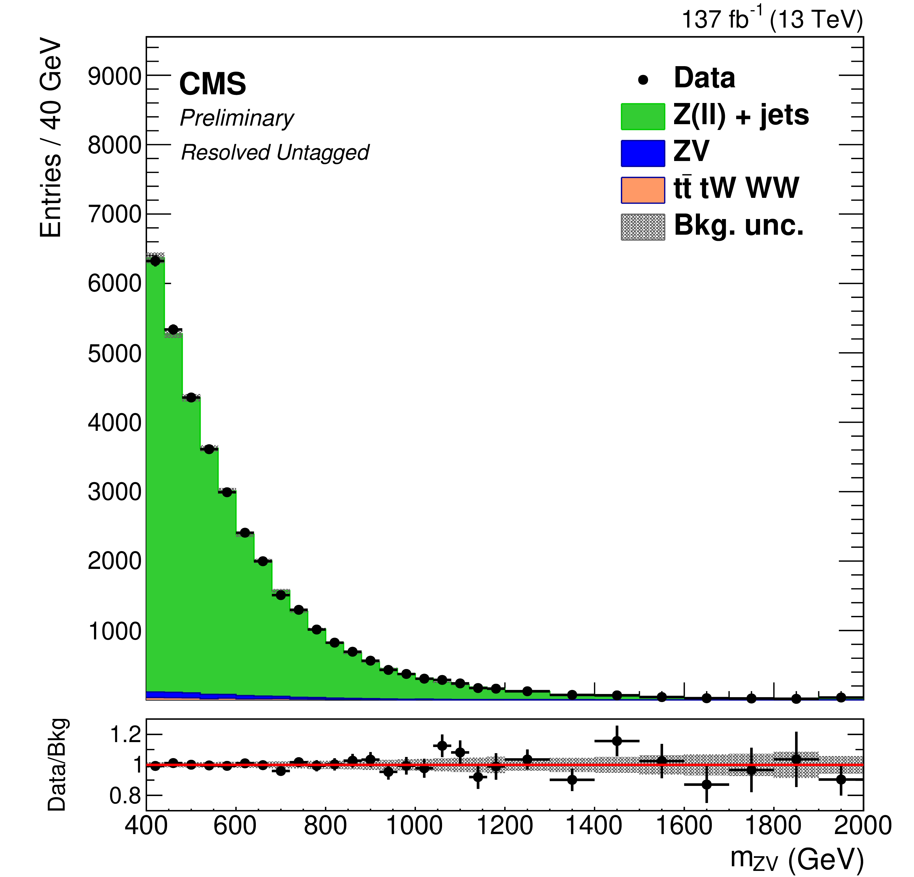
Figure 5:
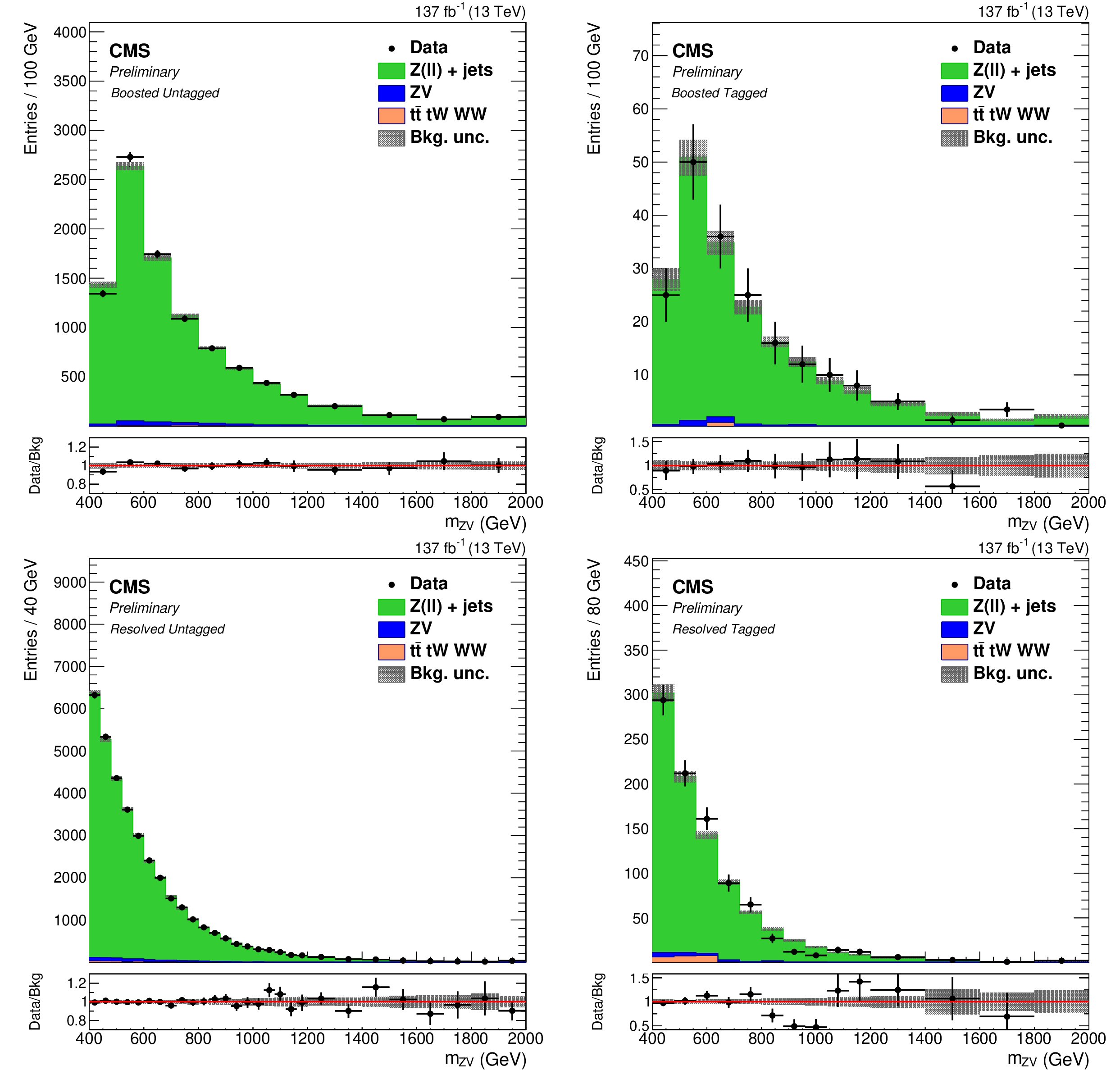
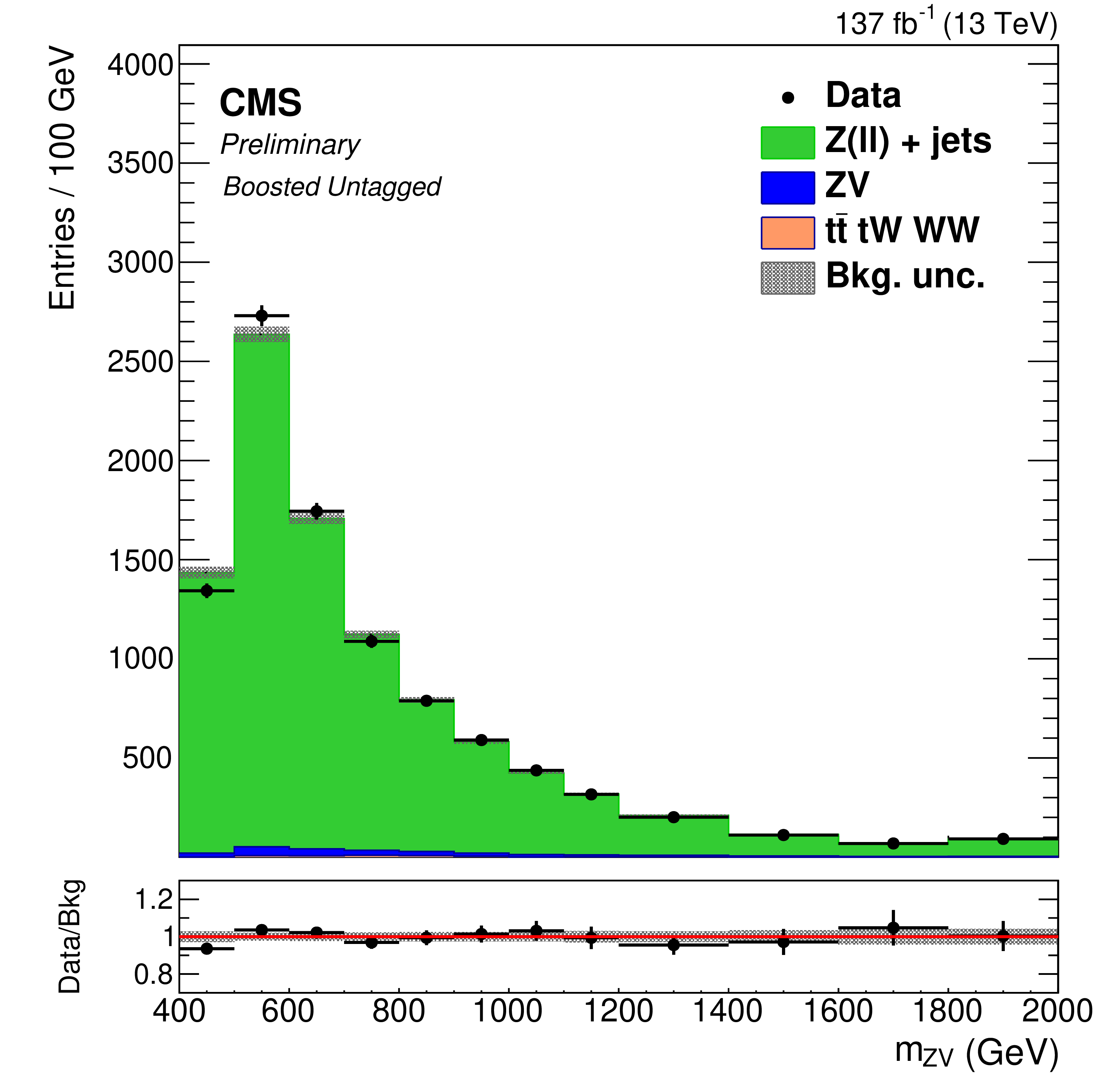
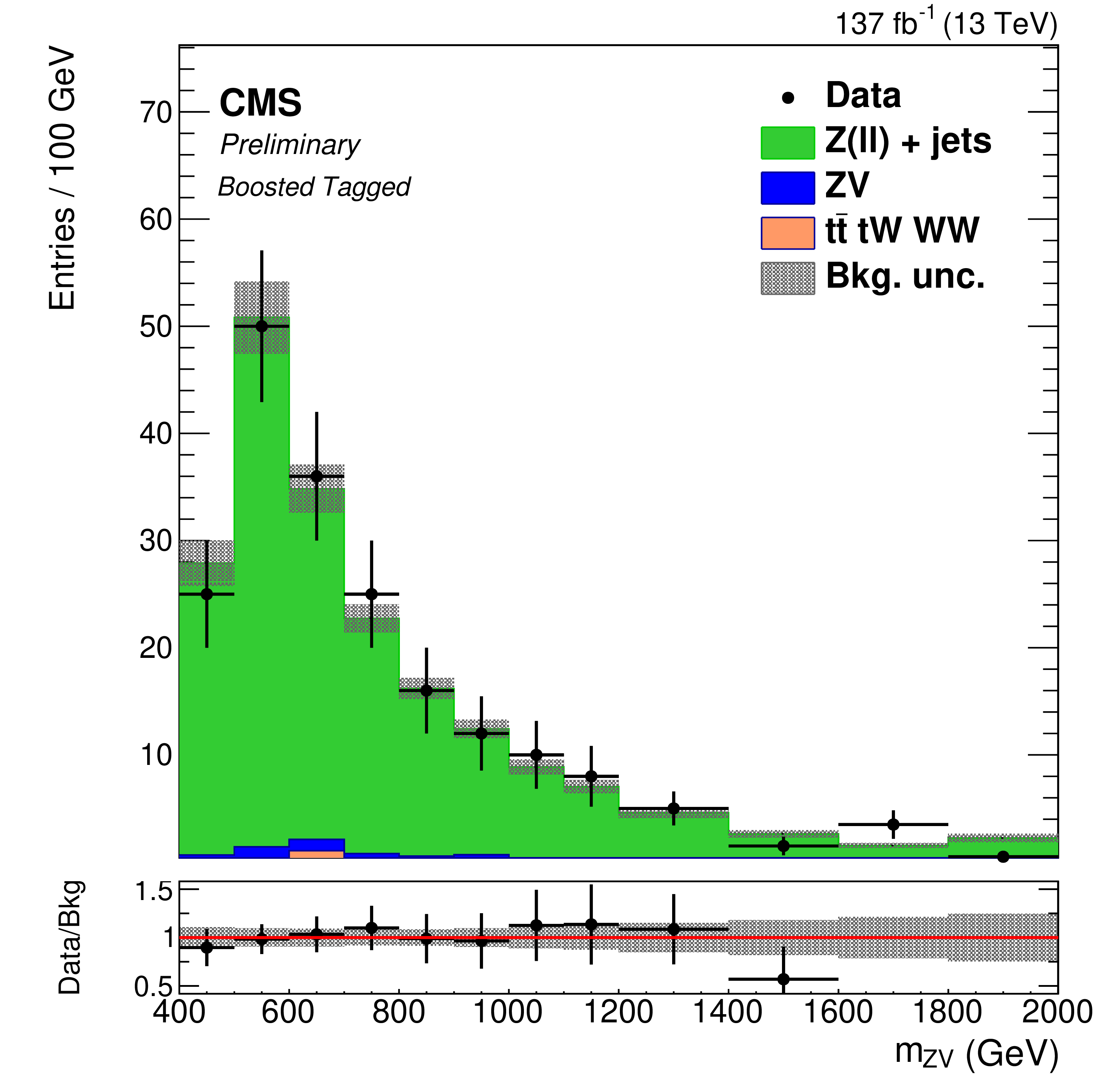
The sideband diboson mass distributions for the boosted V (top), resolved V (bottom), untagged (left), and tagged (right) categories after fitting the sideband data alone. The points show the data, while the filled histograms show the background contributions. The gray band indicates the statistical and postfit systematic uncertainties on the normalization and shape of the background. The lower panel shows the ratio of data to background. |
png pdf |
Figure 5-a:
The sideband diboson mass distributions for the boosted V (top), resolved V (bottom), untagged (left), and tagged (right) categories after fitting the sideband data alone. The points show the data, while the filled histograms show the background contributions. The gray band indicates the statistical and postfit systematic uncertainties on the normalization and shape of the background. The lower panel shows the ratio of data to background. |
png pdf |
Figure 5-b:
The sideband diboson mass distributions for the boosted V (top), resolved V (bottom), untagged (left), and tagged (right) categories after fitting the sideband data alone. The points show the data, while the filled histograms show the background contributions. The gray band indicates the statistical and postfit systematic uncertainties on the normalization and shape of the background. The lower panel shows the ratio of data to background. |
png pdf |
Figure 5-c:
The sideband diboson mass distributions for the boosted V (top), resolved V (bottom), untagged (left), and tagged (right) categories after fitting the sideband data alone. The points show the data, while the filled histograms show the background contributions. The gray band indicates the statistical and postfit systematic uncertainties on the normalization and shape of the background. The lower panel shows the ratio of data to background. |

png pdf |
Figure 5-d:
The sideband diboson mass distributions for the boosted V (top), resolved V (bottom), untagged (left), and tagged (right) categories after fitting the sideband data alone. The points show the data, while the filled histograms show the background contributions. The gray band indicates the statistical and postfit systematic uncertainties on the normalization and shape of the background. The lower panel shows the ratio of data to background. |
png pdf |
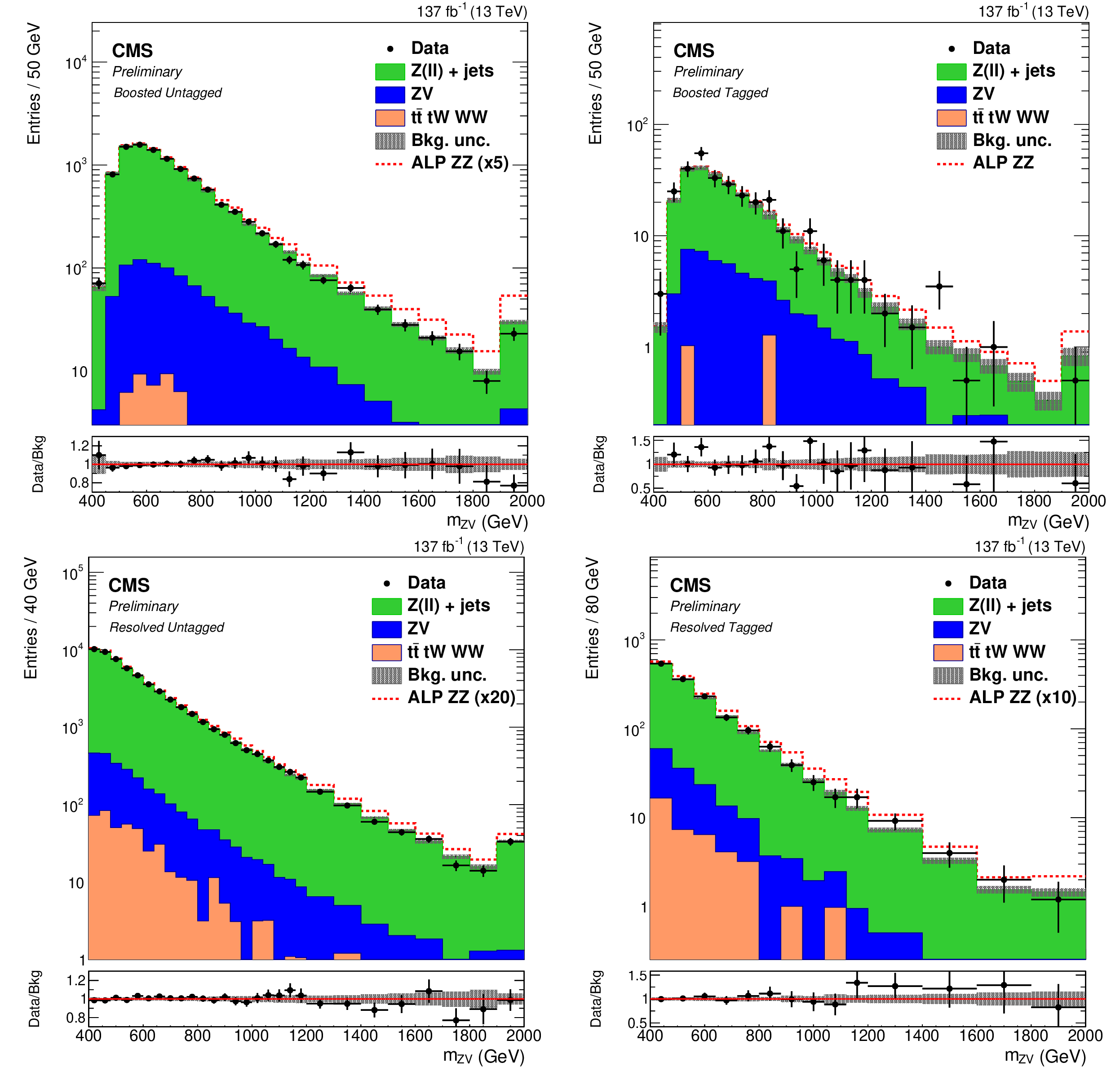
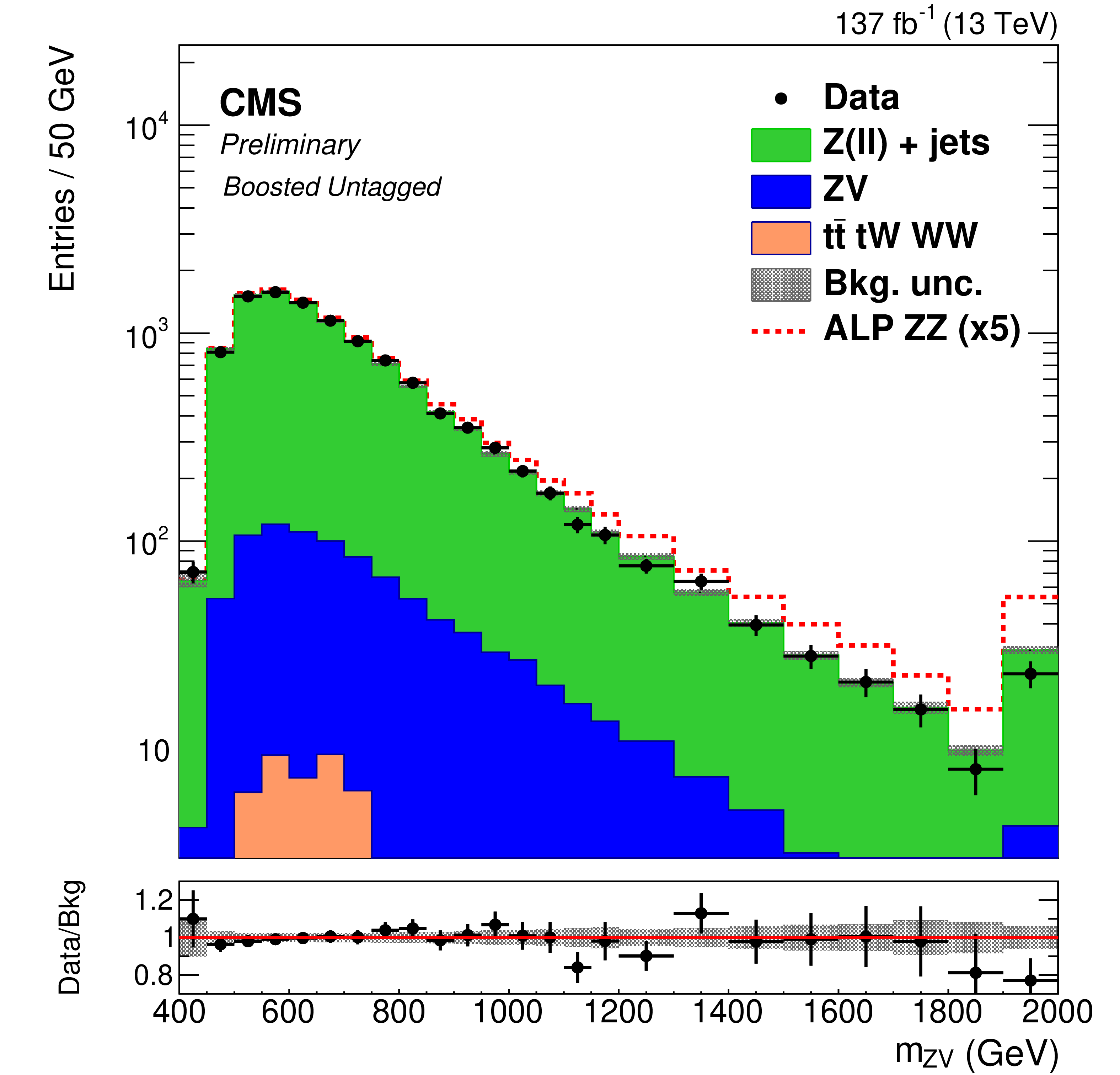
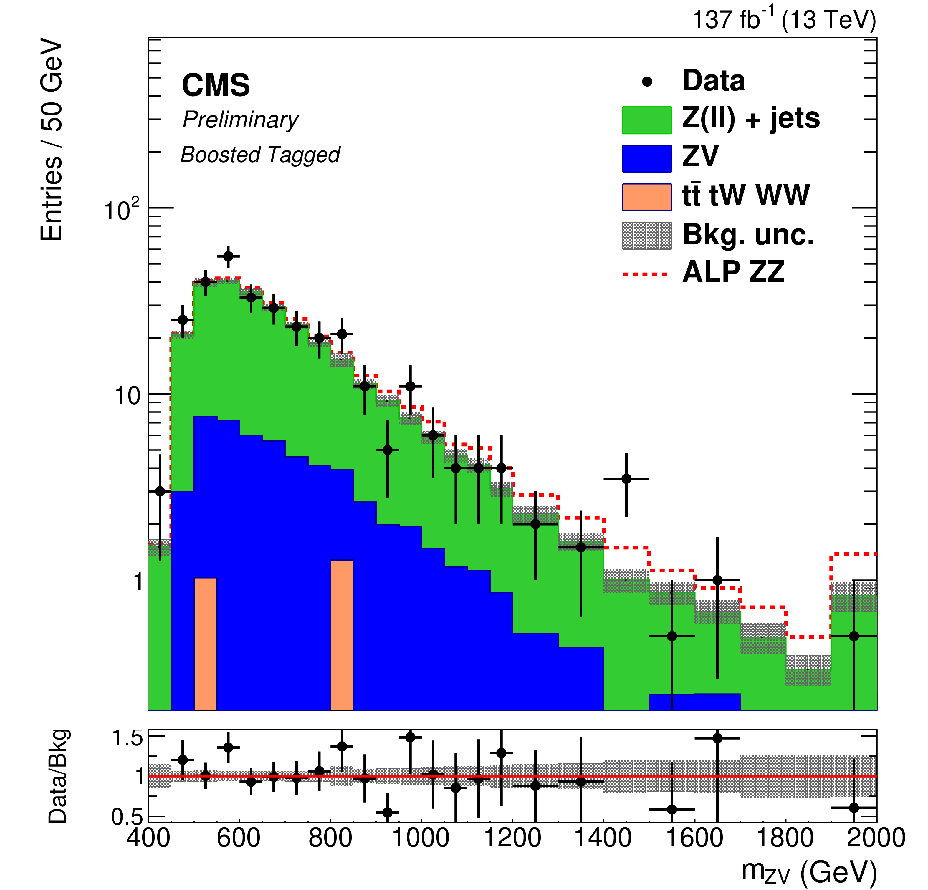
Figure 6:
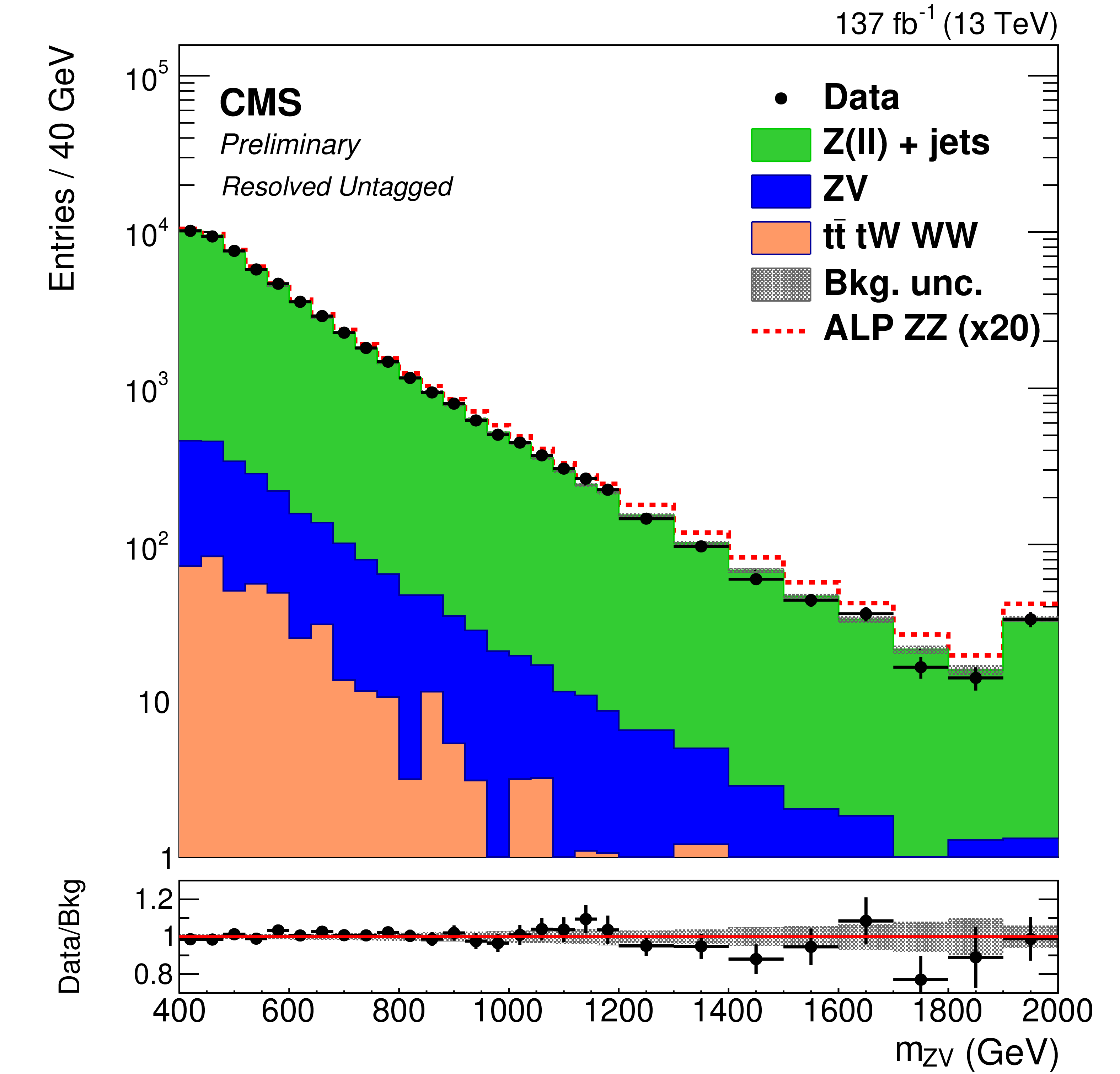
The SR1 ${m_{{\mathrm{Z} \mathrm{V}}}}$ distributions for the boosted V (top), resolved V (bottom), untagged (left), and tagged (right) categories after fitting the signal and sideband regions using a signal (ALP linear ZZ plus background model. The last bin includes events with ${m_{{\mathrm{Z} \mathrm{V}}}}$ values up to 3000 GeV. The points show the data, while the filled histograms show the background contributions. The signal is represented by the red dashed histogram, normalized to the observed 95% CL cross section limit at $f_{\mathrm{a}} = $ 3 TeV. The gray band indicates the statistical and postfit systematic uncertainties on the normalization and shape of the background. The lower panel shows the ratio of data to background. |
png pdf |
Figure 6-a:
The SR1 ${m_{{\mathrm{Z} \mathrm{V}}}}$ distributions for the boosted V (top), resolved V (bottom), untagged (left), and tagged (right) categories after fitting the signal and sideband regions using a signal (ALP linear ZZ plus background model. The last bin includes events with ${m_{{\mathrm{Z} \mathrm{V}}}}$ values up to 3000 GeV. The points show the data, while the filled histograms show the background contributions. The signal is represented by the red dashed histogram, normalized to the observed 95% CL cross section limit at $f_{\mathrm{a}} = $ 3 TeV. The gray band indicates the statistical and postfit systematic uncertainties on the normalization and shape of the background. The lower panel shows the ratio of data to background. |
png pdf |
Figure 6-b:
The SR1 ${m_{{\mathrm{Z} \mathrm{V}}}}$ distributions for the boosted V (top), resolved V (bottom), untagged (left), and tagged (right) categories after fitting the signal and sideband regions using a signal (ALP linear ZZ plus background model. The last bin includes events with ${m_{{\mathrm{Z} \mathrm{V}}}}$ values up to 3000 GeV. The points show the data, while the filled histograms show the background contributions. The signal is represented by the red dashed histogram, normalized to the observed 95% CL cross section limit at $f_{\mathrm{a}} = $ 3 TeV. The gray band indicates the statistical and postfit systematic uncertainties on the normalization and shape of the background. The lower panel shows the ratio of data to background. |
png pdf |
Figure 6-c:
The SR1 ${m_{{\mathrm{Z} \mathrm{V}}}}$ distributions for the boosted V (top), resolved V (bottom), untagged (left), and tagged (right) categories after fitting the signal and sideband regions using a signal (ALP linear ZZ plus background model. The last bin includes events with ${m_{{\mathrm{Z} \mathrm{V}}}}$ values up to 3000 GeV. The points show the data, while the filled histograms show the background contributions. The signal is represented by the red dashed histogram, normalized to the observed 95% CL cross section limit at $f_{\mathrm{a}} = $ 3 TeV. The gray band indicates the statistical and postfit systematic uncertainties on the normalization and shape of the background. The lower panel shows the ratio of data to background. |
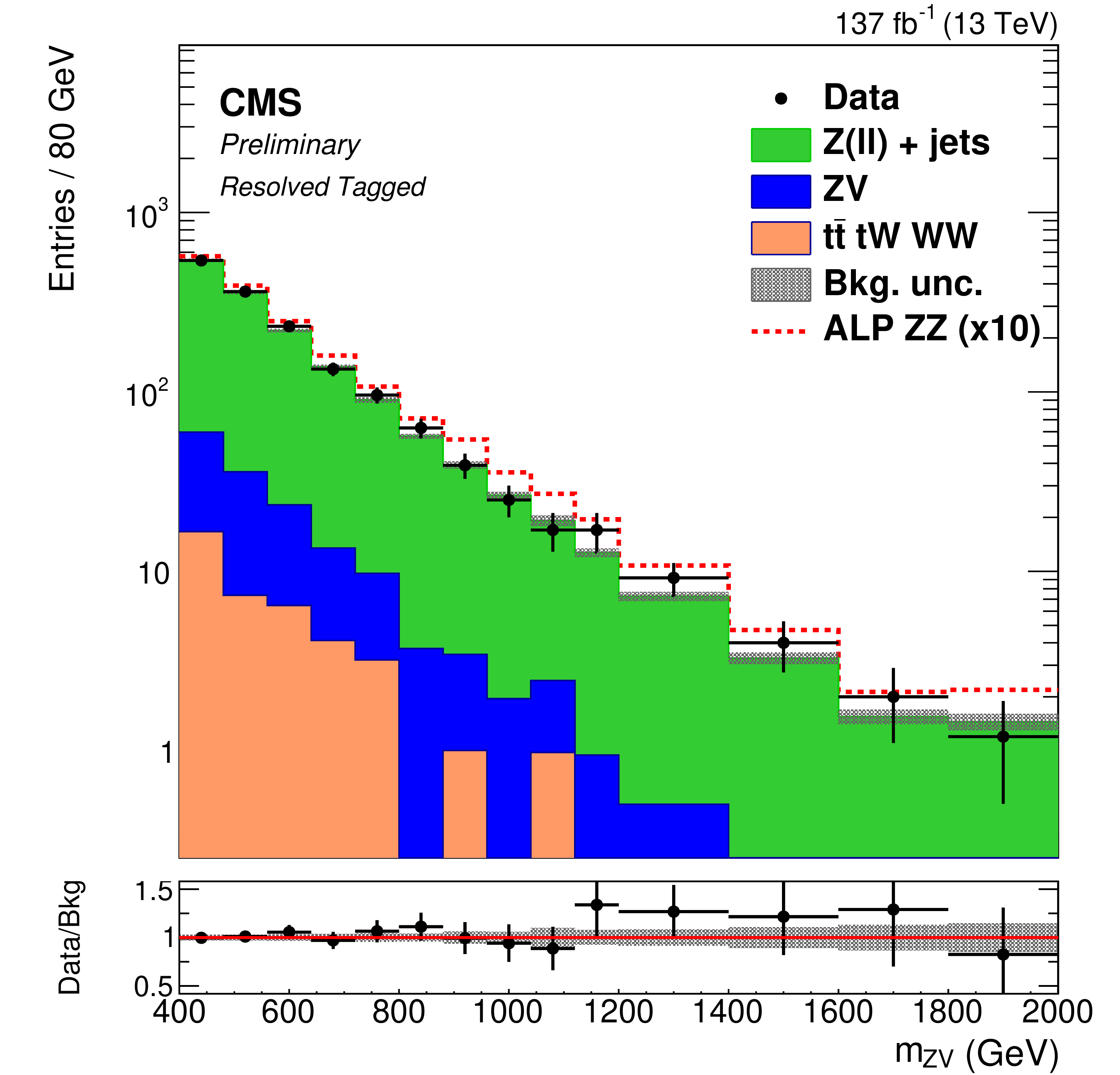
png pdf |
Figure 6-d:
The SR1 ${m_{{\mathrm{Z} \mathrm{V}}}}$ distributions for the boosted V (top), resolved V (bottom), untagged (left), and tagged (right) categories after fitting the signal and sideband regions using a signal (ALP linear ZZ plus background model. The last bin includes events with ${m_{{\mathrm{Z} \mathrm{V}}}}$ values up to 3000 GeV. The points show the data, while the filled histograms show the background contributions. The signal is represented by the red dashed histogram, normalized to the observed 95% CL cross section limit at $f_{\mathrm{a}} = $ 3 TeV. The gray band indicates the statistical and postfit systematic uncertainties on the normalization and shape of the background. The lower panel shows the ratio of data to background. |
png pdf |
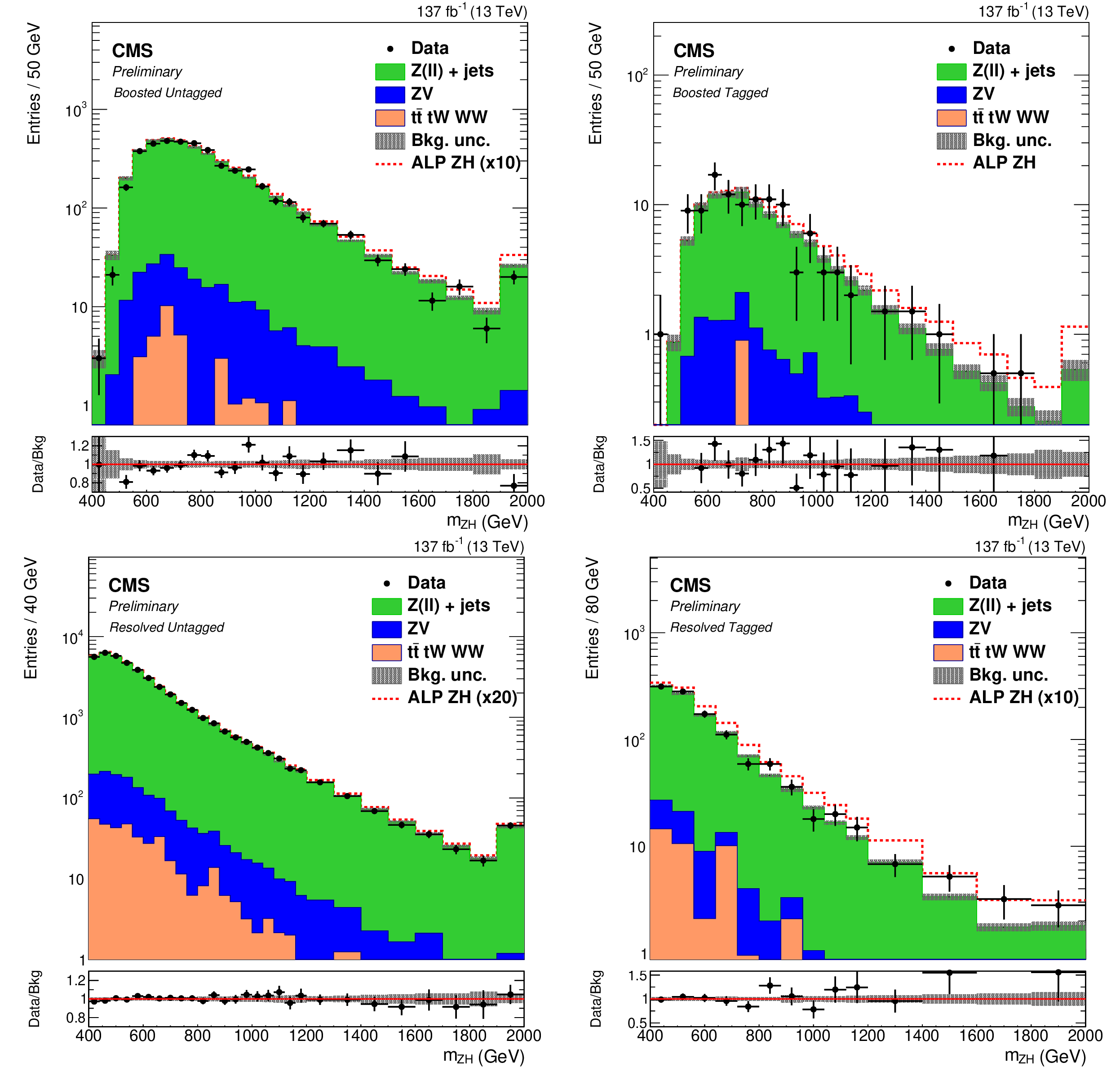
Figure 7:
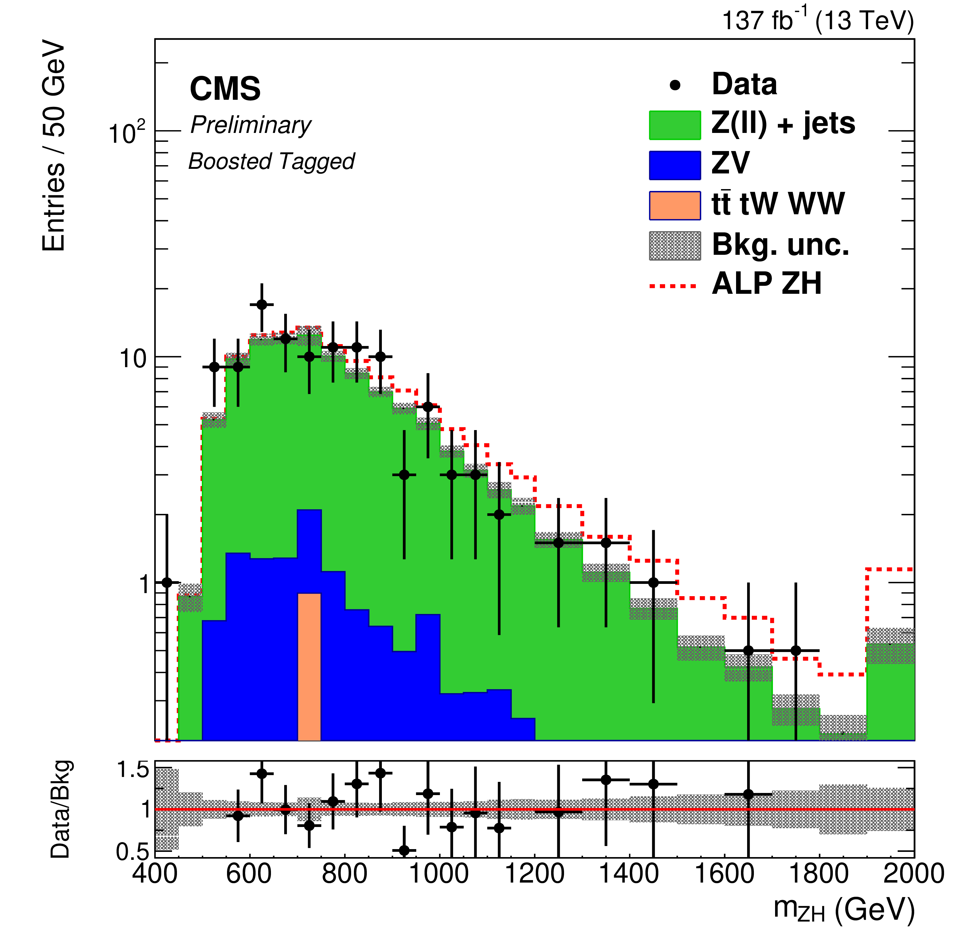
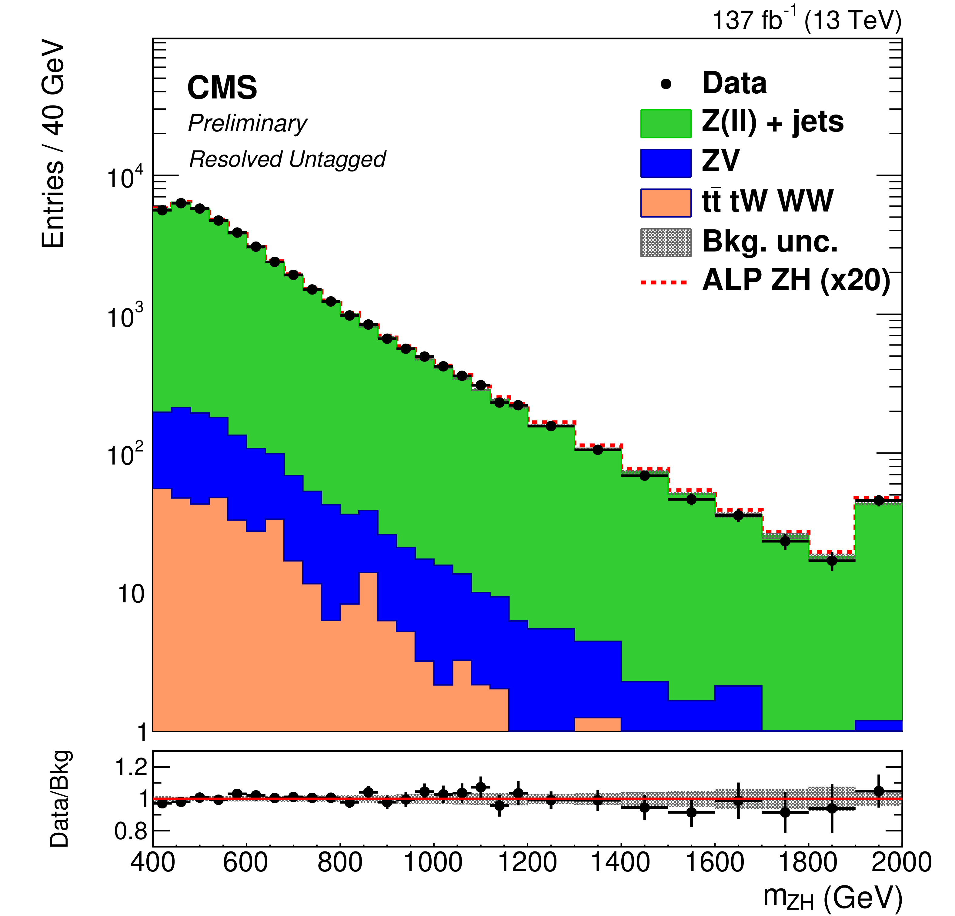
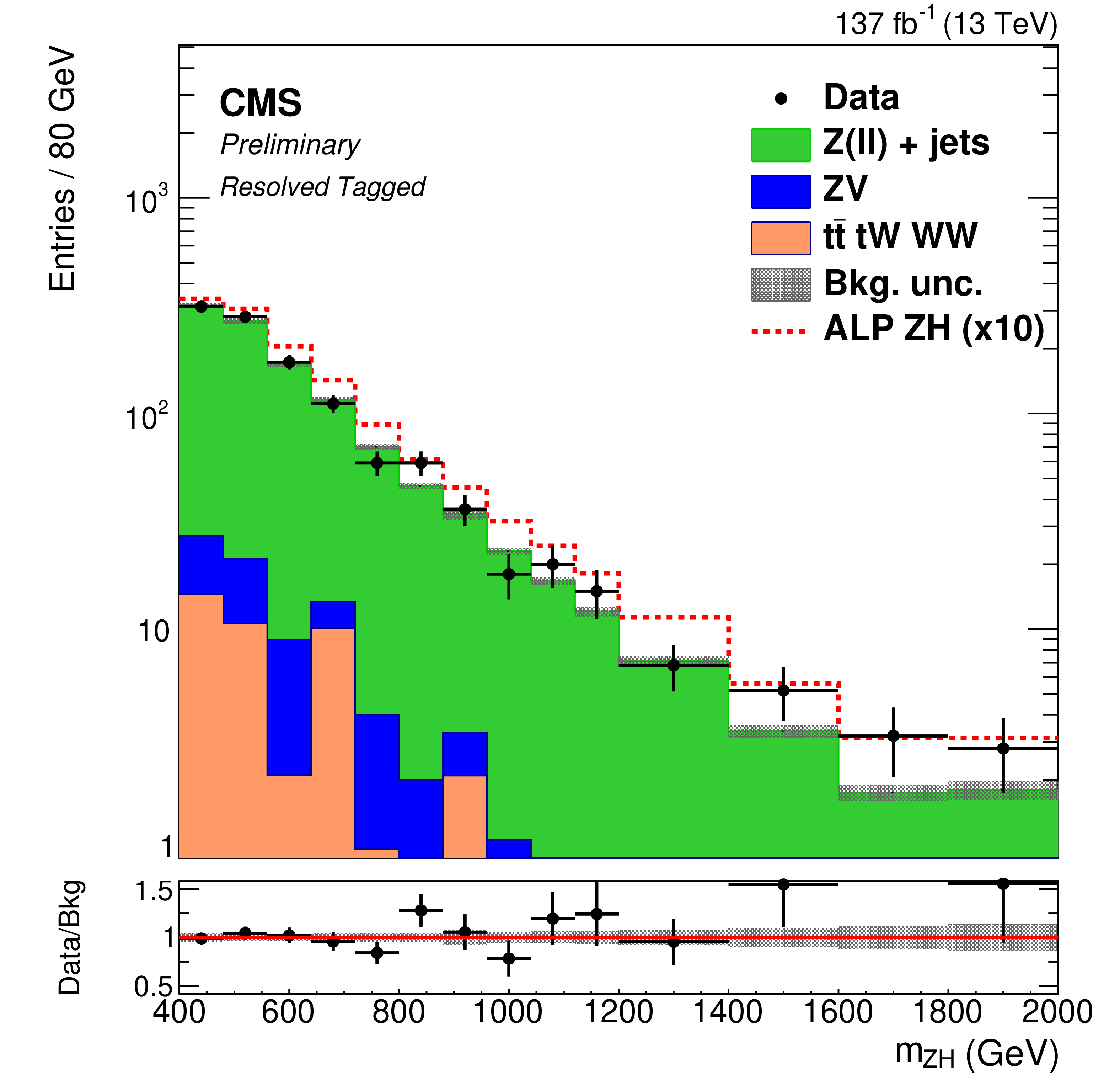
The SR2 ${m_{{\mathrm{Z} \mathrm{H}}}}$ distributions for the boosted H (top), resolved H (bottom), untagged, (left) and tagged (right) categories after fitting the signal and sideband regions using a signal (ALP chiral ZH) plus background model. The last bin includes events with ${m_{{\mathrm{Z} \mathrm{H}}}}$ values up to 3000 GeV. The points show the data while the filled histograms show the background contributions. The signal is represented by the red dashed histogram, normalized to the observed 95% CL cross section limit at $f_{\mathrm{a}} = $ 3 TeV. The gray band indicates the statistical and postfit systematic uncertainties on the normalization and shape of the background. The lower panel shows the ratio of data to background. |
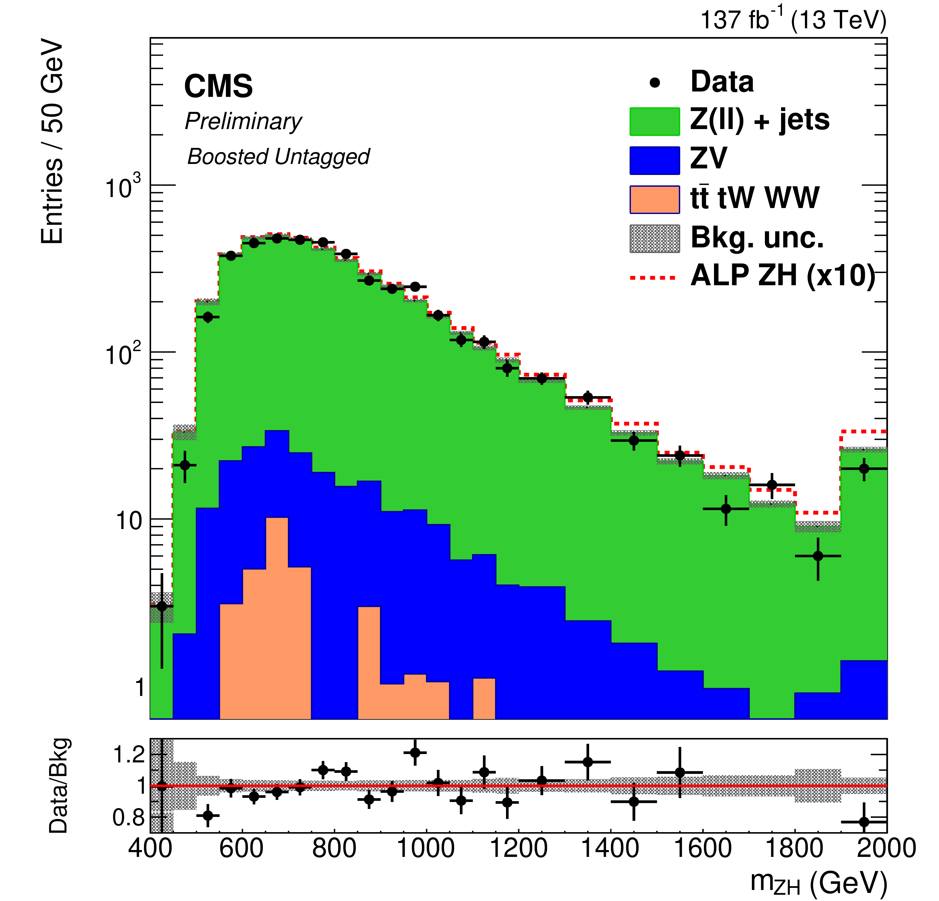
png pdf |
Figure 7-a:
The SR2 ${m_{{\mathrm{Z} \mathrm{H}}}}$ distributions for the boosted H (top), resolved H (bottom), untagged, (left) and tagged (right) categories after fitting the signal and sideband regions using a signal (ALP chiral ZH) plus background model. The last bin includes events with ${m_{{\mathrm{Z} \mathrm{H}}}}$ values up to 3000 GeV. The points show the data while the filled histograms show the background contributions. The signal is represented by the red dashed histogram, normalized to the observed 95% CL cross section limit at $f_{\mathrm{a}} = $ 3 TeV. The gray band indicates the statistical and postfit systematic uncertainties on the normalization and shape of the background. The lower panel shows the ratio of data to background. |
png pdf |
Figure 7-b:
The SR2 ${m_{{\mathrm{Z} \mathrm{H}}}}$ distributions for the boosted H (top), resolved H (bottom), untagged, (left) and tagged (right) categories after fitting the signal and sideband regions using a signal (ALP chiral ZH) plus background model. The last bin includes events with ${m_{{\mathrm{Z} \mathrm{H}}}}$ values up to 3000 GeV. The points show the data while the filled histograms show the background contributions. The signal is represented by the red dashed histogram, normalized to the observed 95% CL cross section limit at $f_{\mathrm{a}} = $ 3 TeV. The gray band indicates the statistical and postfit systematic uncertainties on the normalization and shape of the background. The lower panel shows the ratio of data to background. |
png pdf |
Figure 7-c:
The SR2 ${m_{{\mathrm{Z} \mathrm{H}}}}$ distributions for the boosted H (top), resolved H (bottom), untagged, (left) and tagged (right) categories after fitting the signal and sideband regions using a signal (ALP chiral ZH) plus background model. The last bin includes events with ${m_{{\mathrm{Z} \mathrm{H}}}}$ values up to 3000 GeV. The points show the data while the filled histograms show the background contributions. The signal is represented by the red dashed histogram, normalized to the observed 95% CL cross section limit at $f_{\mathrm{a}} = $ 3 TeV. The gray band indicates the statistical and postfit systematic uncertainties on the normalization and shape of the background. The lower panel shows the ratio of data to background. |
png pdf |
Figure 7-d:
The SR2 ${m_{{\mathrm{Z} \mathrm{H}}}}$ distributions for the boosted H (top), resolved H (bottom), untagged, (left) and tagged (right) categories after fitting the signal and sideband regions using a signal (ALP chiral ZH) plus background model. The last bin includes events with ${m_{{\mathrm{Z} \mathrm{H}}}}$ values up to 3000 GeV. The points show the data while the filled histograms show the background contributions. The signal is represented by the red dashed histogram, normalized to the observed 95% CL cross section limit at $f_{\mathrm{a}} = $ 3 TeV. The gray band indicates the statistical and postfit systematic uncertainties on the normalization and shape of the background. The lower panel shows the ratio of data to background. |

png pdf |
Figure 8:
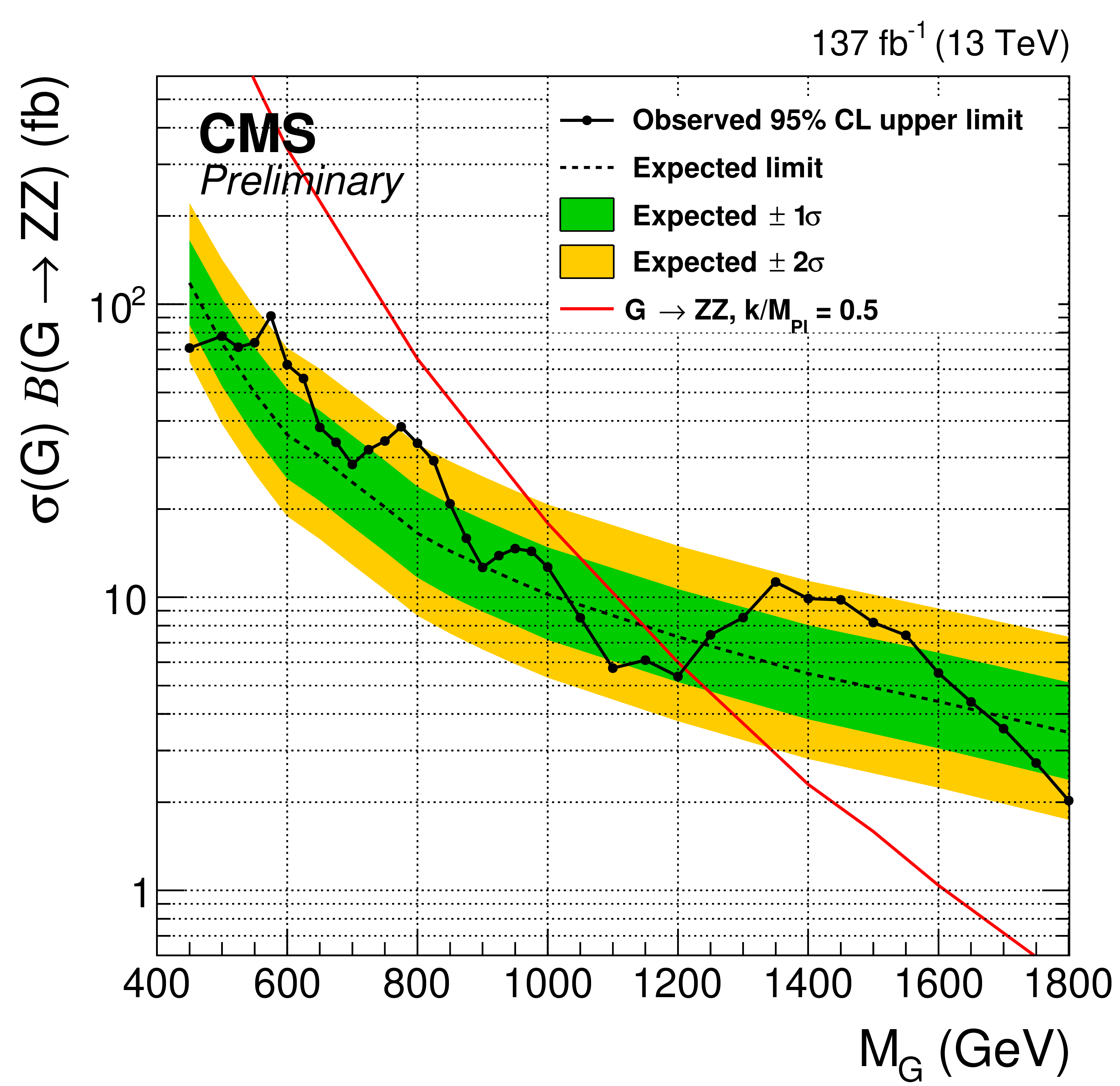
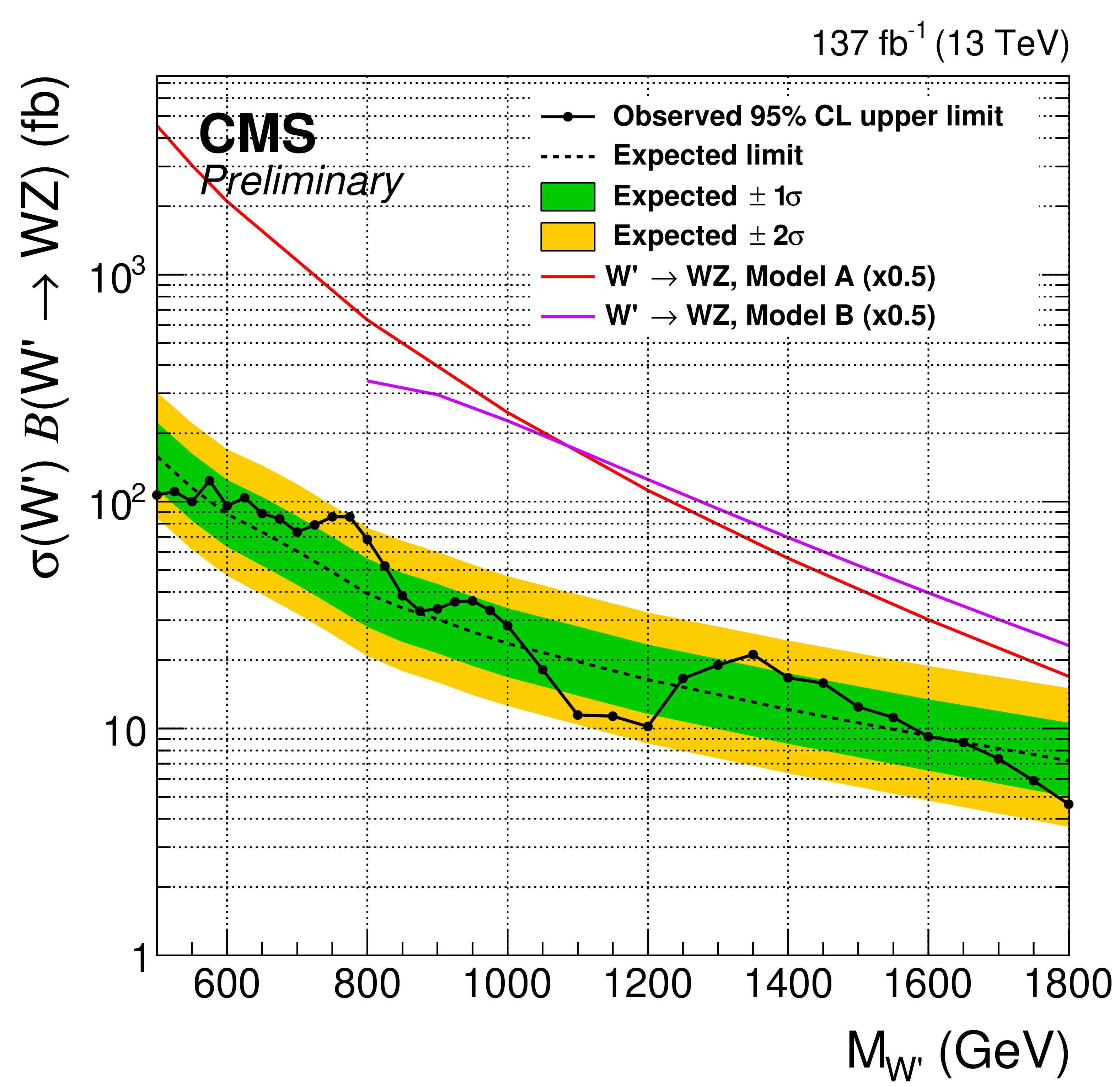
Observed and expected 95% CL upper limits on $\sigma _{\mathrm{G}} \tmspace +\thinmuskip {.1667em} {\mathcal {B}} (\mathrm{G} \to {\mathrm{Z} \mathrm{Z}})$ (left) and $\sigma _{\mathrm{W'}} \tmspace +\thinmuskip {.1667em} {\mathcal {B}} (\mathrm{W'} \to {\mathrm{Z} \mathrm{W}})$ (right) as a function of the resonance mass, taking into account all statistical and systematic uncertainties. The electron and muon channels and the various categories used in the analysis are combined together. The green (inner) and yellow (outer) bands represent the 68% and 95% coverage of the expected limit in the background-only hypothesis. Theoretical predictions for the signal production cross section are also shown: (left) G produced in the WED bulk graviton model with $ \tilde{\kappa} =$ 0.5; (right) W' produced in the framework of HVT model A with $g_\mathrm {v}=$ 1 and model B with $g_\mathrm {v}=$ 3. |
png pdf |
Figure 8-a:
Observed and expected 95% CL upper limits on $\sigma _{\mathrm{G}} \tmspace +\thinmuskip {.1667em} {\mathcal {B}} (\mathrm{G} \to {\mathrm{Z} \mathrm{Z}})$ (left) and $\sigma _{\mathrm{W'}} \tmspace +\thinmuskip {.1667em} {\mathcal {B}} (\mathrm{W'} \to {\mathrm{Z} \mathrm{W}})$ (right) as a function of the resonance mass, taking into account all statistical and systematic uncertainties. The electron and muon channels and the various categories used in the analysis are combined together. The green (inner) and yellow (outer) bands represent the 68% and 95% coverage of the expected limit in the background-only hypothesis. Theoretical predictions for the signal production cross section are also shown: (left) G produced in the WED bulk graviton model with $ \tilde{\kappa} =$ 0.5; (right) W' produced in the framework of HVT model A with $g_\mathrm {v}=$ 1 and model B with $g_\mathrm {v}=$ 3. |
png pdf |
Figure 8-b:
Observed and expected 95% CL upper limits on $\sigma _{\mathrm{G}} \tmspace +\thinmuskip {.1667em} {\mathcal {B}} (\mathrm{G} \to {\mathrm{Z} \mathrm{Z}})$ (left) and $\sigma _{\mathrm{W'}} \tmspace +\thinmuskip {.1667em} {\mathcal {B}} (\mathrm{W'} \to {\mathrm{Z} \mathrm{W}})$ (right) as a function of the resonance mass, taking into account all statistical and systematic uncertainties. The electron and muon channels and the various categories used in the analysis are combined together. The green (inner) and yellow (outer) bands represent the 68% and 95% coverage of the expected limit in the background-only hypothesis. Theoretical predictions for the signal production cross section are also shown: (left) G produced in the WED bulk graviton model with $ \tilde{\kappa} =$ 0.5; (right) W' produced in the framework of HVT model A with $g_\mathrm {v}=$ 1 and model B with $g_\mathrm {v}=$ 3. |
png pdf |
Figure 9:
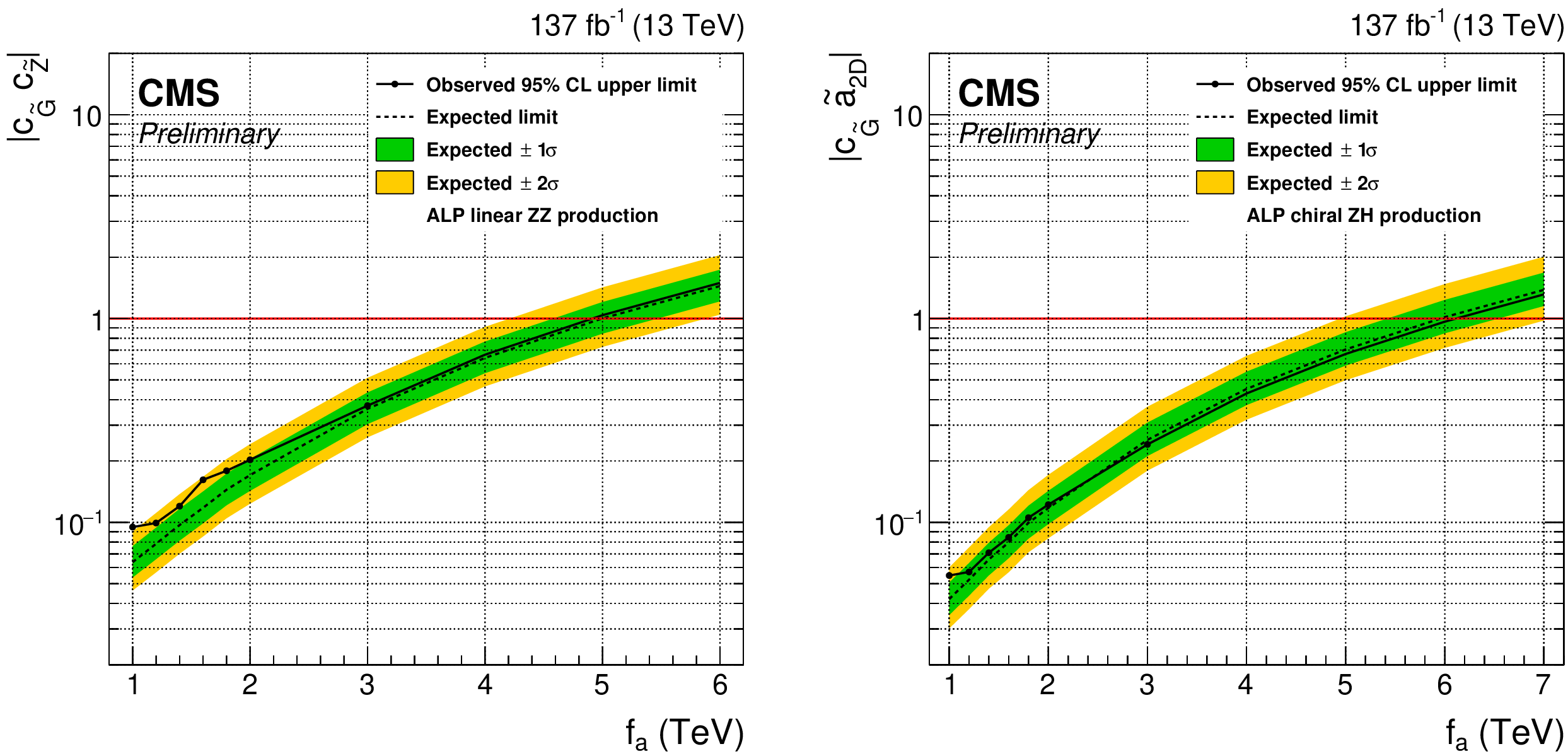
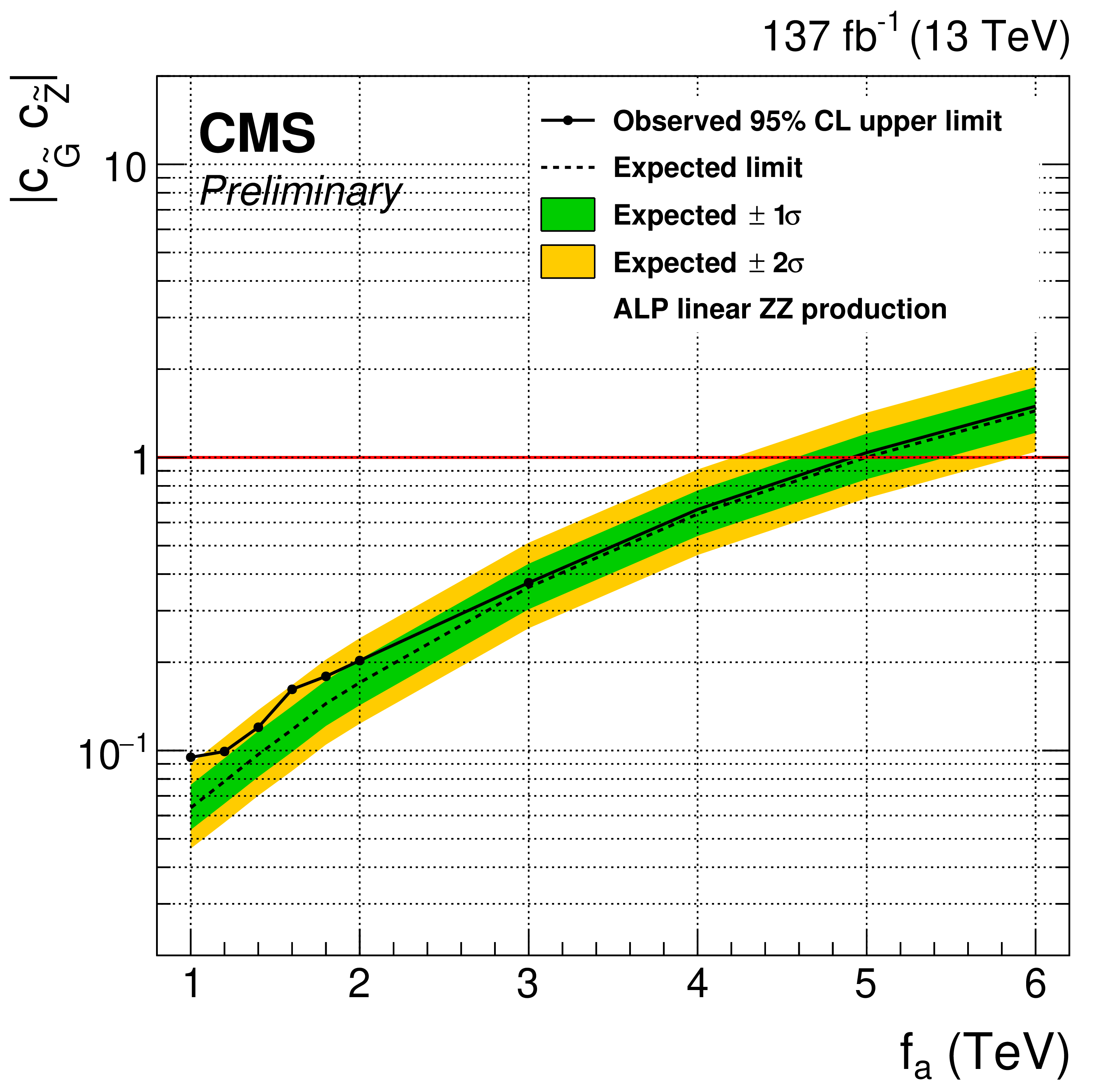
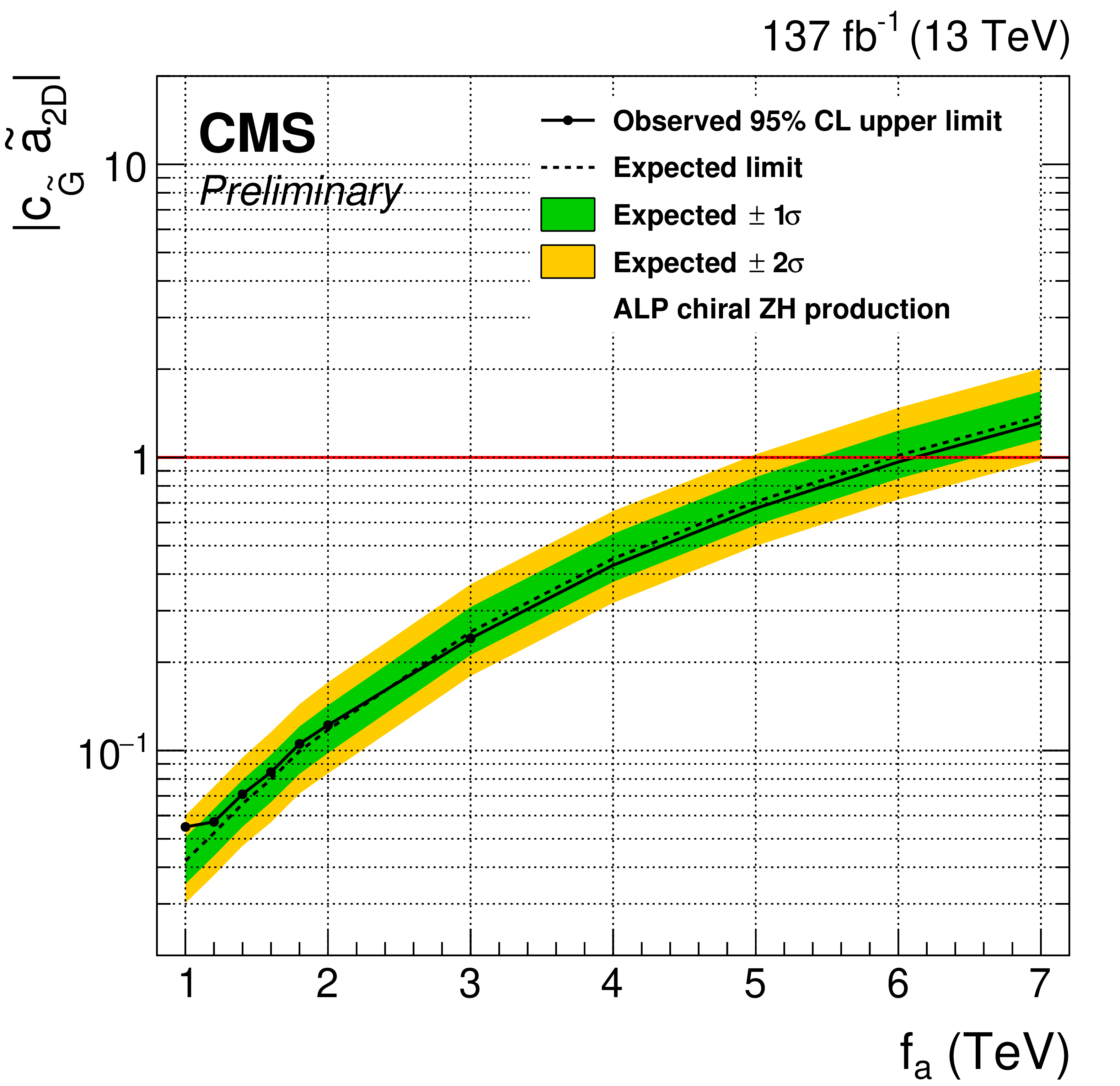
Observed and expected 95% CL upper limits on the ALP linear $ | {c_{\tilde{\mathrm{G}}}} {c_{\tilde{\mathrm{Z}}}} | $ (left) and the ALP chiral $ | {c_{\tilde{\mathrm{G}}}} {\tilde{a}_{\text {2D}}} | $ (right) couplings as a function of the mass scale $f_{\mathrm{a}} $ for ALP masses $m_{\mathrm{a}} < $ 100 GeV. |
png pdf |
Figure 9-a:
Observed and expected 95% CL upper limits on the ALP linear $ | {c_{\tilde{\mathrm{G}}}} {c_{\tilde{\mathrm{Z}}}} | $ (left) and the ALP chiral $ | {c_{\tilde{\mathrm{G}}}} {\tilde{a}_{\text {2D}}} | $ (right) couplings as a function of the mass scale $f_{\mathrm{a}} $ for ALP masses $m_{\mathrm{a}} < $ 100 GeV. |
png pdf |
Figure 9-b:
Observed and expected 95% CL upper limits on the ALP linear $ | {c_{\tilde{\mathrm{G}}}} {c_{\tilde{\mathrm{Z}}}} | $ (left) and the ALP chiral $ | {c_{\tilde{\mathrm{G}}}} {\tilde{a}_{\text {2D}}} | $ (right) couplings as a function of the mass scale $f_{\mathrm{a}} $ for ALP masses $m_{\mathrm{a}} < $ 100 GeV. |
| Tables | |
png pdf |
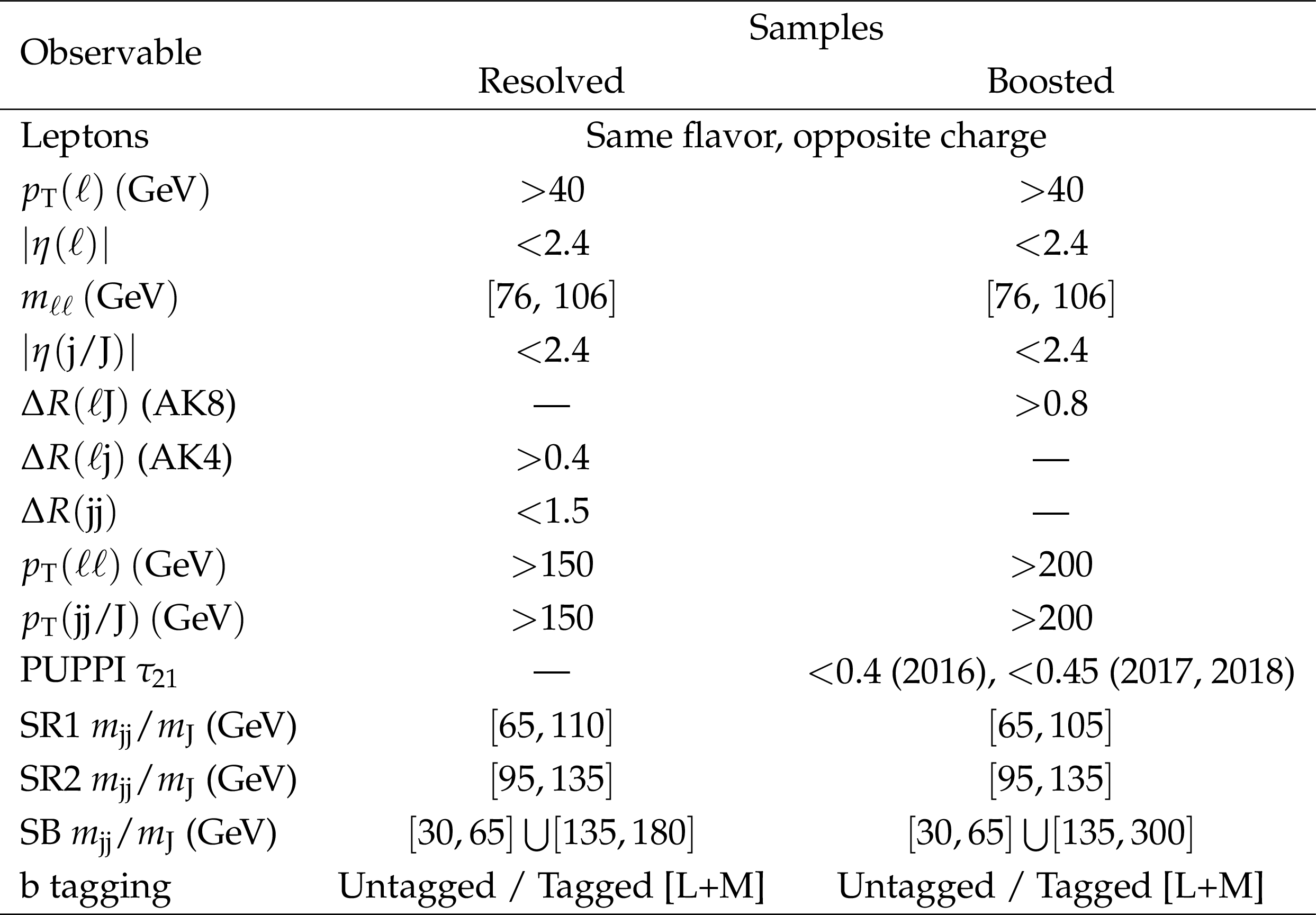
Table 1:
Summary of selection requirements and categorization. |

png pdf |
Table 2:
Summary of systematic uncertainties, quoted in percent, affecting the normalization of background and signal samples. Where a systematic uncertainty depends on the signal ZV or ZH final state or mass, the smallest and largest values are reported in the table. In the case of a systematic uncertainty applying only to a specific background source, the source is indicated in parentheses. Systematic uncertainties too small to be considered are written as "$ < $0.1", while a dash (--) represents uncertainties not applicable in the specific analysis category. |
png pdf |
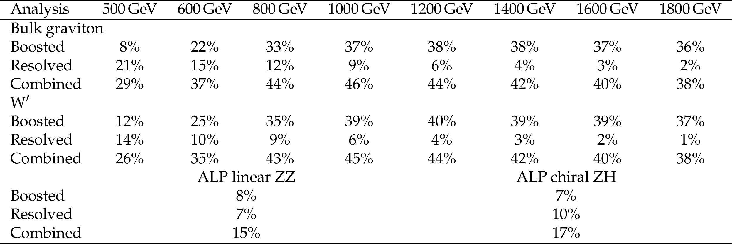
Table 3:
Selection efficiencies for the bulk graviton, W', and ALP linear and chiral models. |
png pdf |
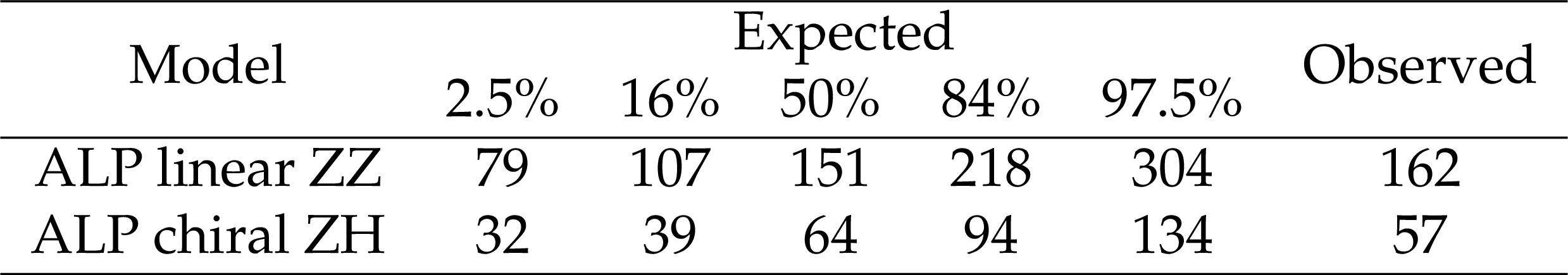
Table 4:
Expected and observed 95% CL$_{\text{s}}$ upper limits on $\sigma (\mathrm{g} \mathrm{g} \to \mathrm{a}^{*} \to \mathrm{Z} \mathrm{Z} / \mathrm{Z} \mathrm{H})$ in fb for $f_{\mathrm{a}} = $ 3 TeV. |
| Summary |
|
A search for heavy resonances and nonresonant ALPs in semileptonic ZZ, ZW, or ZH final states has been presented. The analysis is sensitive to resonances with masses in the range from 450 to 1800 GeV decaying into ZZ or ZW. A search for the effects of nonresonant ALP-mediated ZZ or ZH production has been included. Two categories are defined based on the merged or resolved reconstruction of the hadronically decaying boson. The search is based on data collected from 2016 to 2018 by the CMS experiment at the LHC in proton-proton collisions with a center-of-mass energy of 13 TeV, corresponding to an integrated luminosity of 137 fb$^{-1}$. No excess is observed in the data above the standard model expectations. Depending on the resonance mass, upper limits of 2-90 fb and 5-120 fb have been set on the product of the cross section of a spin-2 bulk graviton and the ZZ branching fraction, and on a spin-1 W' signal and the ZW branching fraction, respectively. These limits improve on those previously obtained by the CMS collaboration in the analogous final states [11]. Upper limits on the nonresonant ALP-mediated ZZ and ZH production cross sections for a scale $f_{\mathrm{a}} = $ 3 TeV and ALP masses $m_{\mathrm{a}} < $ 100 GeV have been established at 162 fb and 57 fb, respectively. Depending on the value of the scale $f_{\mathrm{a}}$, upper limits on the product of the ALP coupling to gluons with the relevant coupling to ZZ or ZH of 0.02-0.09 TeV$^{-2}$ have been set, valid for ALP masses $m_{\mathrm{a}} < $ 100 GeV. These are the first limits based on nonresonant ALP-mediated ZZ and ZH production obtained by the LHC experiments. |
| References | ||||
| 1 | K. Agashe, H. Davoudiasl, G. Perez, and A. Soni | Warped gravitons at the LHC and beyond | PRD 76 (2007) 036006 | hep-ph/0701186 |
| 2 | L. Randall and R. Sundrum | A large mass hierarchy from a small extra dimension | PRL 83 (1999) 3370 | hep-ph/9905221 |
| 3 | L. Randall and R. Sundrum | An alternative to compactification | PRL 83 (1999) 4690 | hep-th/9906064 |
| 4 | D. Pappadopulo, A. Thamm, R. Torre, and A. Wulzer | Heavy vector triplets: Bridging theory and data | JHEP 09 (2014) 060 | 1402.4431 |
| 5 | H. Georgi, D. B. Kaplan, and L. Randall | Manifesting the invisible axion at low energies | PLB 169 (1986) 73 | |
| 6 | K. Choi, K. Kang, and J. E. Kim | Effects of $ \eta^\prime $ in low-energy axion physics | PLB 181 (1986) 145 | |
| 7 | I. Brivio et al. | ALPs effective field theory and collider signatures | EPJC 77 (2017) 572 | |
| 8 | M. Bauer, M. Neubert, and A. Thamm | Collider probes of axion-like particles | JHEP 12 (2017) 044 | |
| 9 | M. B. Gavela, J. M. No, V. Sanz, and J. F. de Troc\'oniz | Non-resonant searches for axion-like particles at the LHC | PRL 124 (2020) 051802 | |
| 10 | CMS Collaboration | Search for a heavy resonance decaying into a Z boson and a vector boson in the $ \nu \overline{\nu}\mathrm{q}\overline{\mathrm{q}} $ final state | JHEP 07 (2018) 075 | CMS-B2G-17-005 1803.03838 |
| 11 | CMS Collaboration | Search for a heavy resonance decaying into a Z boson and a Z or W boson in 2$ \ell2q $ final states at $ \sqrt{s}= $ 13 TeV | JHEP 09 (2018) 101 | CMS-B2G-17-013 1803.10093 |
| 12 | CMS Collaboration | Combination of CMS searches for heavy resonances decaying to pairs of bosons or leptons | PLB 798 (2019) 134952 | CMS-B2G-18-006 1906.00057 |
| 13 | ATLAS Collaboration | Search for heavy diboson resonances in semileptonic final states in $ pp $ collisions at $ \sqrt{s}= $ 13 TeV with the ATLAS detector | EPJC 80 (2020) 1165 | 2004.14636 |
| 14 | CMS Collaboration | Search for a heavy vector resonance decaying to a Z boson and a Higgs boson in proton-proton collisions at $ \sqrt{s} = $ 13 TeV | Submitted to EPJC | CMS-B2G-19-006 2102.08198 |
| 15 | S. Carra et al. | Constraining off-shell production of axion-like particles with $ Z\gamma $ and $ WW $ differential cross-section measurements | 2106.10085 | |
| 16 | A. L. Fitzpatrick, J. Kaplan, L. Randall, and L.-T. Wang | Searching for the Kaluza-Klein graviton in bulk RS models | JHEP 09 (2007) 013 | hep-ph/0701150 |
| 17 | W. D. Goldberger and M. B. Wise | Modulus stabilization with bulk fields | PRL 83 (1999) 4922 | hep-ph/9907447 |
| 18 | A. Carvalho | Gravity particles from warped extra dimensions, predictions for LHC | 1404.0102 | |
| 19 | J. Alwall et al. | The automated computation of tree-level and next-to-leading order differential cross sections, and their matching to parton shower simulations | JHEP 07 (2014) 079 | 1405.0301 |
| 20 | W. Buchmuller and D. Wyler | Effective Lagrangian analysis of new interactions and flavor conservation | NPB 268 (1986) 621 | |
| 21 | B. Grzadkowski, et al. | Dimension-six terms in the standard model Lagrangian | JHEP 1010 (2010) 085 | |
| 22 | F. Feruglio | The chiral approach to the electroweak interactions | Int. J. Mod. Phys. A 8 (1993) 4937 | |
| 23 | A. Azatov, R. Contino, and J. Galloway | Model-independent bounds on a light Higgs | JHEP 1204 (2012) 127 | |
| 24 | R. Alonso et al. | The effective chiral Lagrangian for a light dynamical Higgs particle | PLB 722 (2013) 330 | |
| 25 | G. Buchalla, O. Cat\`a, and C. Krause | Complete electroweak chiral Lagrangian with a light Higgs at NLO | NPB 880 (2014) 552 | |
| 26 | J. M. Lindert et al. | Precise predictions for $ {V}+ $ jets dark matter backgrounds | EPJC 77 (2017) 829 | 1705.04664 |
| 27 | T. Sjostrand et al. | An introduction to PYTHIA 8.2 | CPC 191 (2015) 159--177 | 1410.3012 |
| 28 | CMS Collaboration | Event generator tunes obtained from underlying event and multiparton scattering measurements | EPJC 76 (2016) 155 | CMS-GEN-14-001 1512.00815 |
| 29 | CMS Collaboration | Extraction and validation of a new set of CMS PYTHIA8 tunes from underlying-event measurements | EPJC 80 (2020), no. 1, 4 | CMS-GEN-17-001 1903.12179 |
| 30 | NNPDF Collaboration | Parton distributions for the LHC Run II | JHEP 04 (2015) 040 | 1410.8849 |
| 31 | NNPDF Collaboration | Parton distributions from high-precision collider data | EPJC 77 (2017) 663 | 1706.00428 |
| 32 | GEANT4 Collaboration | GEANT4--a simulation toolkit | NIMA 506 (2003) 250 | |
| 33 | CMS Collaboration | Performance of the CMS level-1 trigger in proton-proton collisions at $ \sqrt{s} = $ 13 TeV | JINST 15 (2020) P10017 | CMS-TRG-17-001 2006.10165 |
| 34 | CMS Collaboration | The CMS trigger system | JINST 12 (2017) P01020 | CMS-TRG-12-001 1609.02366 |
| 35 | CMS Collaboration | The CMS experiment at the CERN LHC | JINST 3 (2008) S08004 | CMS-00-001 |
| 36 | CMS Collaboration | Particle-flow reconstruction and global event description with the CMS detector | JINST 12 (2017) P10003 | CMS-PRF-14-001 1706.04965 |
| 37 | M. Cacciari, G. P. Salam, and G. Soyez | The anti-$ {k_{\mathrm{T}}} $ jet clustering algorithm | JHEP 04 (2008) 063 | 0802.1189 |
| 38 | M. Cacciari, G. P. Salam, and G. Soyez | FastJet user manual | EPJC 72 (2012) 1896 | 1111.6097 |
| 39 | CMS Collaboration | Description and performance of track and primary-vertex reconstruction with the CMS tracker | JINST 9 (2014) P10009 | CMS-TRK-11-001 1405.6569 |
| 40 | CMS Tracker Group Collaboration | The CMS phase-1 pixel detector upgrade | JINST 16 (2021) P02027 | 2012.14304 |
| 41 | CMS Collaboration | Track impact parameter resolution for the full pseudo rapidity coverage in the 2017 dataset with the CMS phase-1 pixel detector | CDS | |
| 42 | CMS Collaboration | Performance of electron reconstruction and selection with the CMS detector in proton-proton collisions at $ \sqrt{s} = $ 8 TeV | JINST 10 (2015) P06005 | CMS-EGM-13-001 1502.02701 |
| 43 | CMS Collaboration | Performance of the CMS muon detector and muon reconstruction with proton-proton collisions at $ \sqrt{s} = $ 13 TeV | JINST 13 (2018) P06015 | CMS-MUO-16-001 1804.04528 |
| 44 | CMS Collaboration | Pileup mitigation at CMS in 13 TeV data | JINST 15 (2020) P09018 | CMS-JME-18-001 2003.00503 |
| 45 | D. Bertolini, P. Harris, M. Low, and N. Tran | Pileup per particle identification | JHEP 10 (2014) 059 | 1407.6013 |
| 46 | CMS Collaboration | Jet energy scale and resolution in the CMS experiment in pp collisions at 8 TeV | JINST 12 (2017) P02014 | CMS-JME-13-004 1607.03663 |
| 47 | M. Dasgupta, A. Fregoso, S. Marzani, and G. P. Salam | Towards an understanding of jet substructure | JHEP 09 (2013) 029 | 1307.0007 |
| 48 | A. J. Larkoski, S. Marzani, G. Soyez, and J. Thaler | Soft drop | JHEP 05 (2014) 146 | 1402.2657 |
| 49 | J. Thaler and K. Van Tilburg | Identifying boosted objects with N-subjettiness | JHEP 03 (2011) 015 | 1011.2268 |
| 50 | CMS Collaboration | Identification of heavy-flavour jets with the CMS detector in pp collisions at 13 TeV | JINST 13 (2018) P05011 | CMS-BTV-16-002 1712.07158 |
| 51 | CMS Collaboration | Jet algorithms performance in 13 TeV data | CMS-PAS-JME-16-003 | CMS-PAS-JME-16-003 |
| 52 | CMS Collaboration | Identification techniques for highly boosted W bosons that decay into hadrons | JHEP 12 (2014) 017 | CMS-JME-13-006 1410.4227 |
| 53 | J. Butterworth et al. | PDF4LHC recommendations for LHC Run II | JPG 43 (2016) 023001 | 1510.03865 |
| 54 | CMS Collaboration | CMS luminosity measurement for the 2016 data taking period | CMS-PAS-LUM-17-001 | CMS-PAS-LUM-17-001 |
| 55 | CMS Collaboration | CMS luminosity measurement for the 2017 data-taking period at $ \sqrt{s} = $ 13 TeV | CMS-PAS-LUM-17-004 | CMS-PAS-LUM-17-004 |
| 56 | CMS Collaboration | CMS luminosity measurement for the 2018 data-taking period at $ \sqrt{s} = $ 13 TeV | CMS-PAS-LUM-18-002 | CMS-PAS-LUM-18-002 |
| 57 | A. L. Read | Presentation of search results: The CL$ _{\text{s}} $ technique | JPG 28 (2002) 2693 | |
| 58 | T. Junk | Confidence level computation for combining searches with small statistics | NIMA 434 (1999) 435 | hep-ex/9902006 |
| 59 | G. Cowan, K. Cranmer, E. Gross, and O. Vitells | Asymptotic formulae for likelihood-based tests of new physics | EPJC 71 (2011) 1554 | 1007.1727 |
| 60 | The ATLAS Collaboration, The CMS Collaboration, The LHC Higgs Combination Group | Procedure for the LHC Higgs boson search combination in Summer 2011 | CMS-NOTE-2011-005 | |
|
|
Compact Muon Solenoid LHC, CERN |
|

|

|

|

|

|