

Compact Muon Solenoid
LHC, CERN
| CMS-PAS-B2G-18-002 | ||
| Search for heavy resonances in the all-hadronic vector-boson pair final state with a multi-dimensional fit | ||
| CMS Collaboration | ||
| March 2019 | ||
| Abstract: We present a novel fit method in the search for new resonances decaying to WW, WZ, or ZZ boson pairs in the all-hadronic final state using data corresponding to an integrated luminosity of 77.3 fb$^{-1}$ taken with the CMS experiment at the LHC at a centre-of-mass energy of $\sqrt{s}= $ 13 TeV. The search is focussed on resonances with masses above 1.2 TeV, where the decay products of each W or Z boson are expected to be collimated into one single large-radius jet. The signal extraction method is based on a three-dimensional maximum likelihood fit of the dijet invariant mass and the two jet masses, which allows systematic uncertainties that affect all three dimensions to be incorporated simultaneously. The new method yields an improvement in sensitivity of up to 30% with respect to previous search methods used in CMS. No excess is observed above the estimated standard model background. In a heavy vector triplet model, spin-1 W' and Z' resonances with masses below 3.8 and 3.5 TeV, respectively, are excluded at 95% confidence level. In a narrow-width bulk graviton model, upper limits on cross sections are set between 27 and 0.2 fb for resonance masses between 1.2 and 5.2 TeV, respectively. | ||
|
Links:
CDS record (PDF) ;
CADI line (restricted) ;
These preliminary results are superseded in this paper, EPJC 80 (2020) 237. The superseded preliminary plots can be found here. |
||
| Figures | |
png pdf |
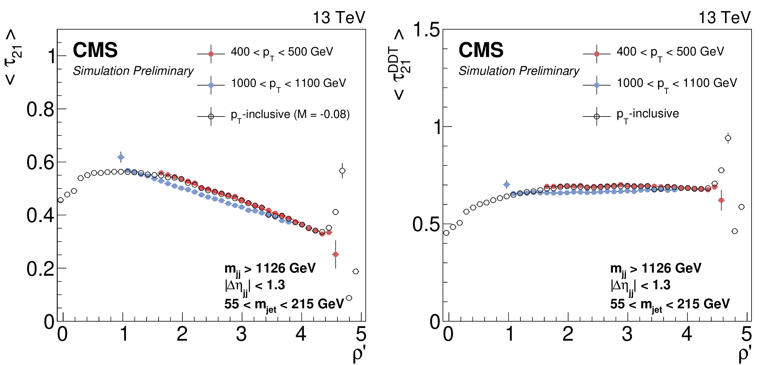
Figure 1:
The ${\tau _{21}}$ profile dependence on $\rho ' = \log({m_\mathrm {jet}} ^2/ {p_{\mathrm {T}}} /\mu)$ (left). A fit to the linear part of the spectrum yields the slope $M =-0.080$, which is used to define the mass- and ${p_{\mathrm {T}}}$ -decorrelated variable $ {\tau _{21}^\textbf {DDT}} = {\tau _{21}} -M\times \rho '$. The ${\tau _{21}^\textbf {DDT}}$ profile versus $\rho '$ is shown on the right. |
png pdf |
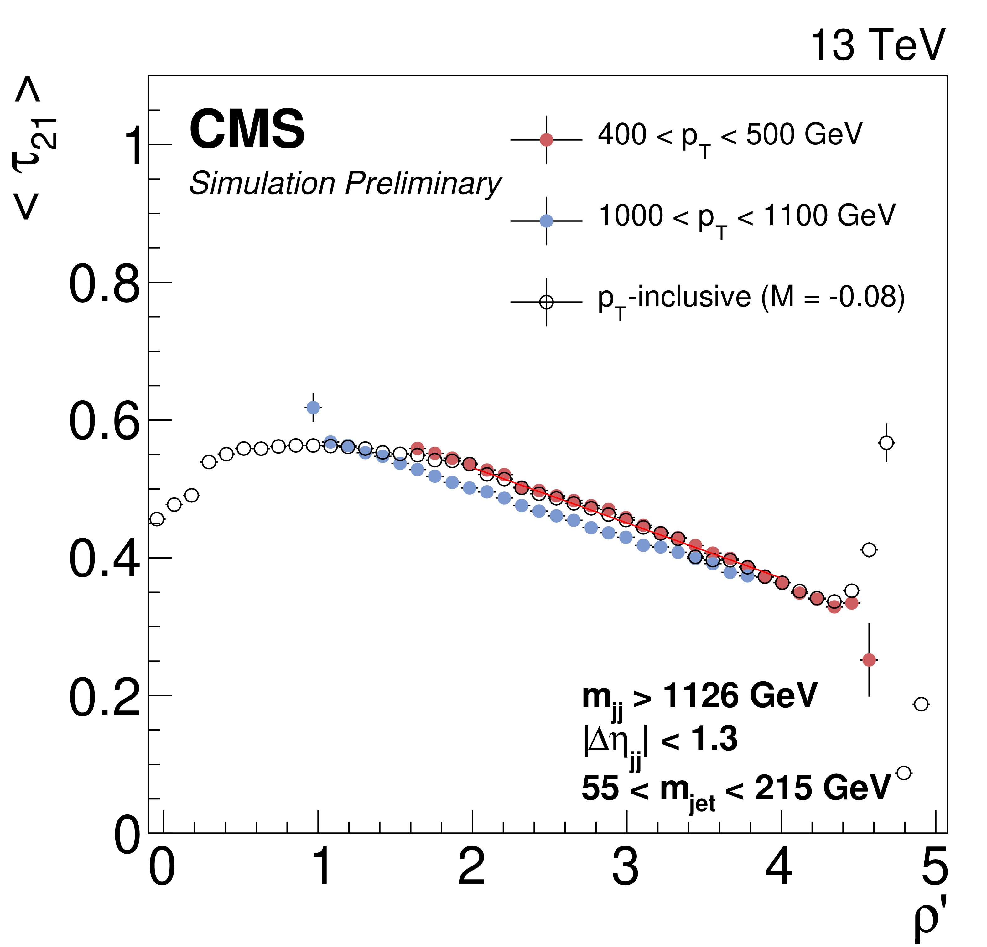
Figure 1-a:
The ${\tau _{21}}$ profile dependence on $\rho ' = \log({m_\mathrm {jet}} ^2/ {p_{\mathrm {T}}} /\mu)$. A fit to the linear part of the spectrum yields the slope $M =-0.080$, which is used to define the mass- and ${p_{\mathrm {T}}}$ -decorrelated variable $ {\tau _{21}^\textbf {DDT}} = {\tau _{21}} -M\times \rho '$. |
png pdf |
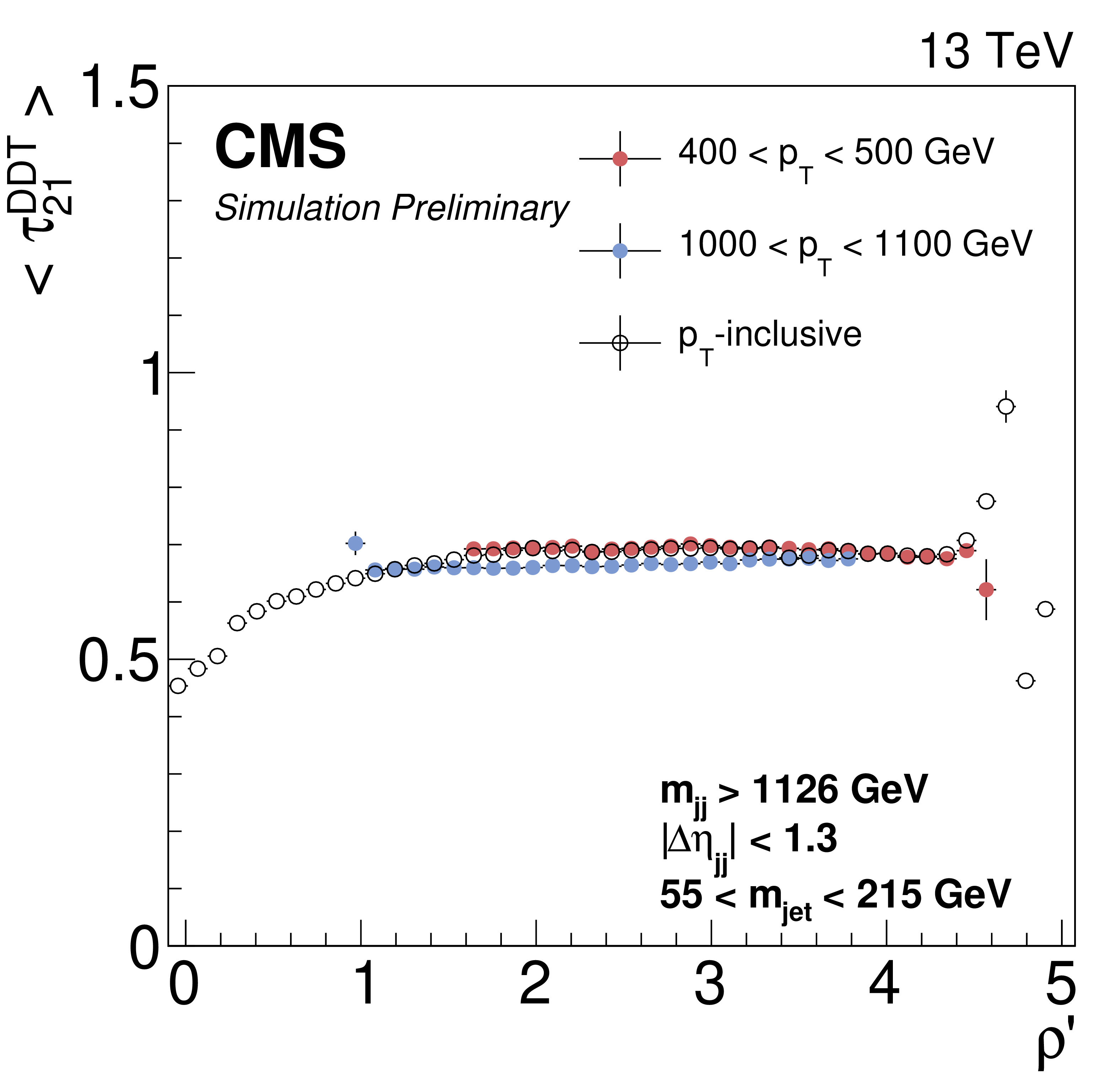
Figure 1-b:
The ${\tau _{21}^\textbf {DDT}}$ profile versus $\rho '$ is shown. |
png pdf |
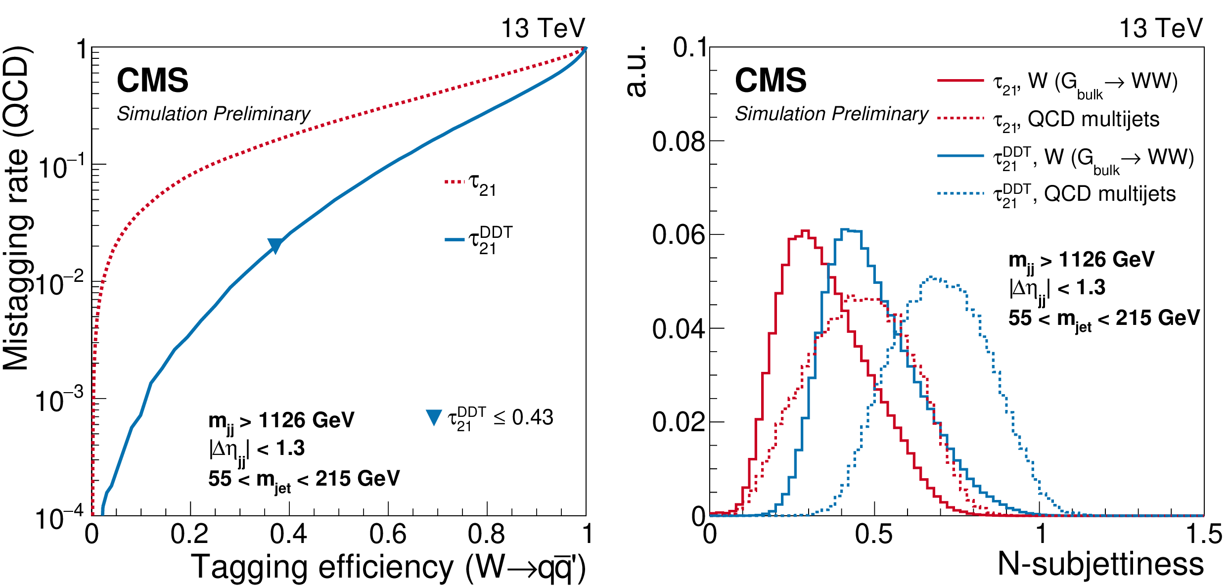
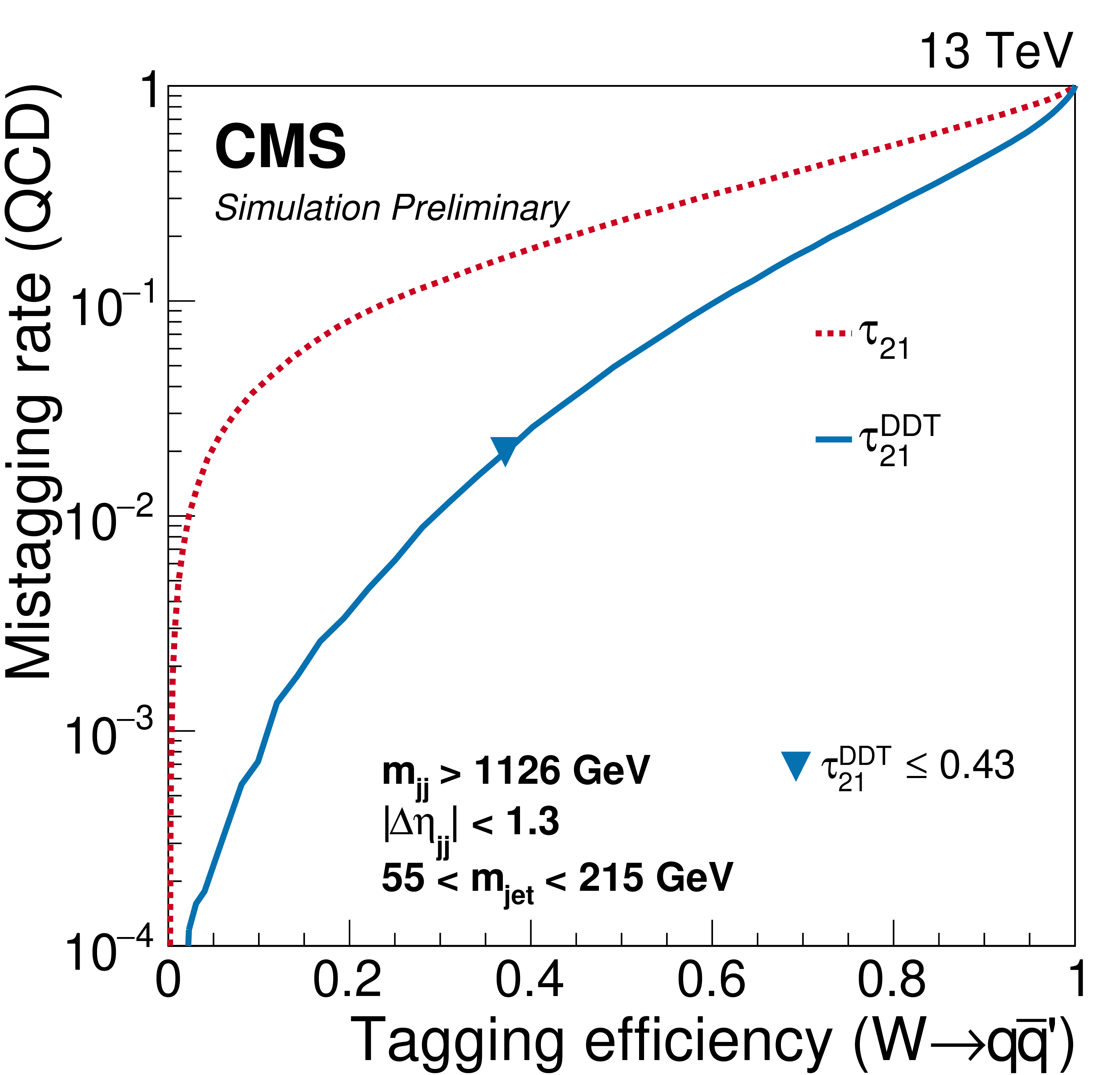
Figure 2:
Left: Performance of ${\tau _{21}}$ and ${\tau _{21}^\textbf {DDT}}$ in the background-signal efficiency plane. Right: Distribution of ${\tau _{21}}$ and ${\tau _{21}^\textbf {DDT}}$ for W-jets and quark or gluon jets from QCD multijet events. |
png pdf |
Figure 2-a:
Performance of ${\tau _{21}}$ and ${\tau _{21}^\textbf {DDT}}$ in the background-signal efficiency plane. |

png pdf |
Figure 2-b:
Distribution of ${\tau _{21}}$ and ${\tau _{21}^\textbf {DDT}}$ for W-jets and quark or gluon jets from QCD multijet events. |
png pdf |
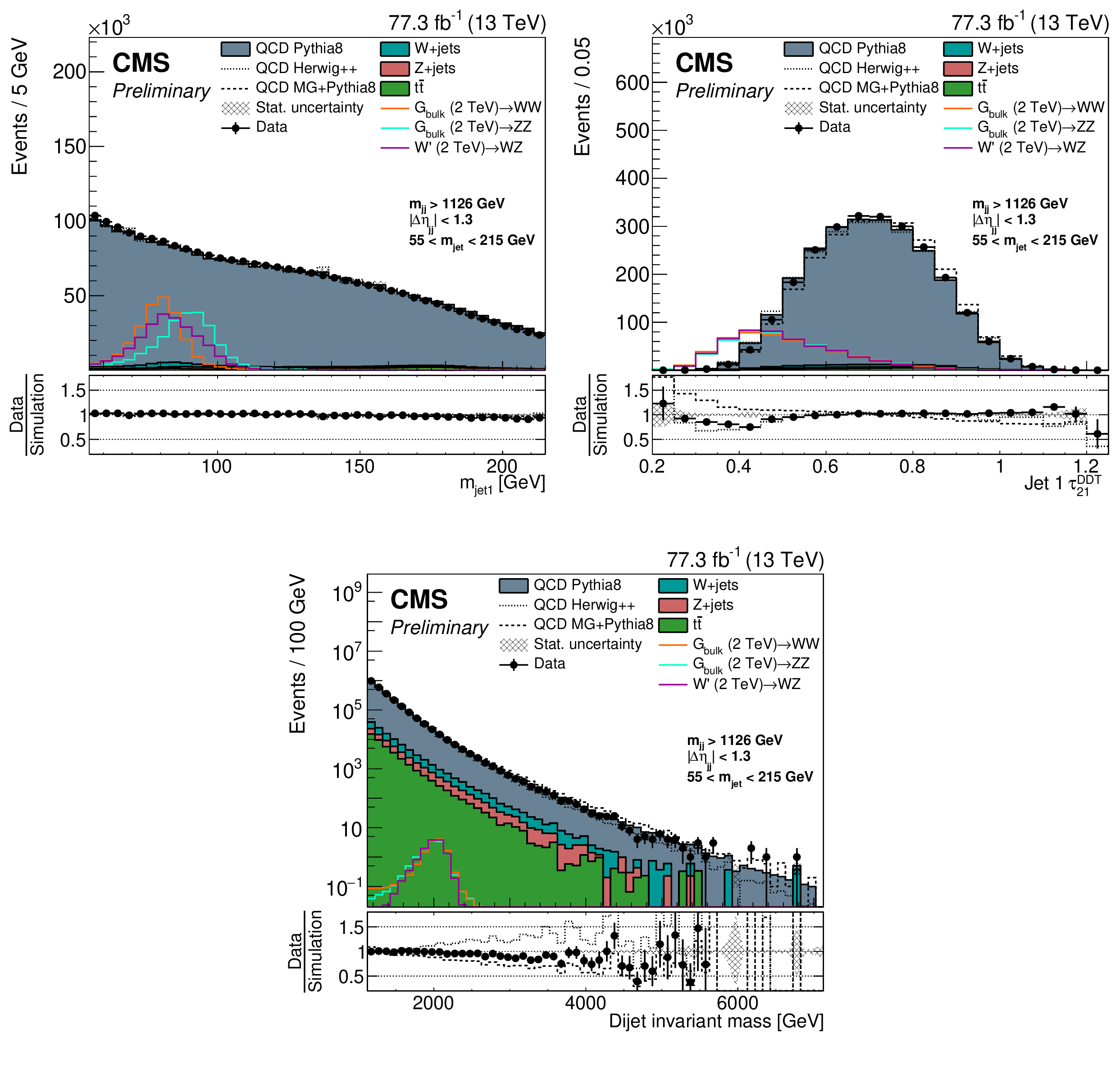
Figure 3:
Jet mass (upper left) and ${\tau _{21}^\textbf {DDT}}$ (upper right) distributions for randomly sorted selected jets, and dijet invariant mass distribution (lower) for events with a jet mass between 55 and 215 GeV in data and simulation. For the QCD multijet simulation, several alternative predictions are shown, scaled to the data minus the other background processes, which are scaled to their SM expectation as described in the text. The different signal distributions are arbitrarily scaled for visibility. No selection on ${\tau _{21}^\textbf {DDT}}$ is applied. |

png pdf |
Figure 3-a:
Jet mass distribution for randomly sorted selected jets for events with a jet mass between 55 and 215 GeV in data and simulation. For the QCD multijet simulation, several alternative predictions are shown, scaled to the data minus the other background processes, which are scaled to their SM expectation as described in the text. The different signal distributions are arbitrarily scaled for visibility. No selection on ${\tau _{21}^\textbf {DDT}}$ is applied. |
png pdf |
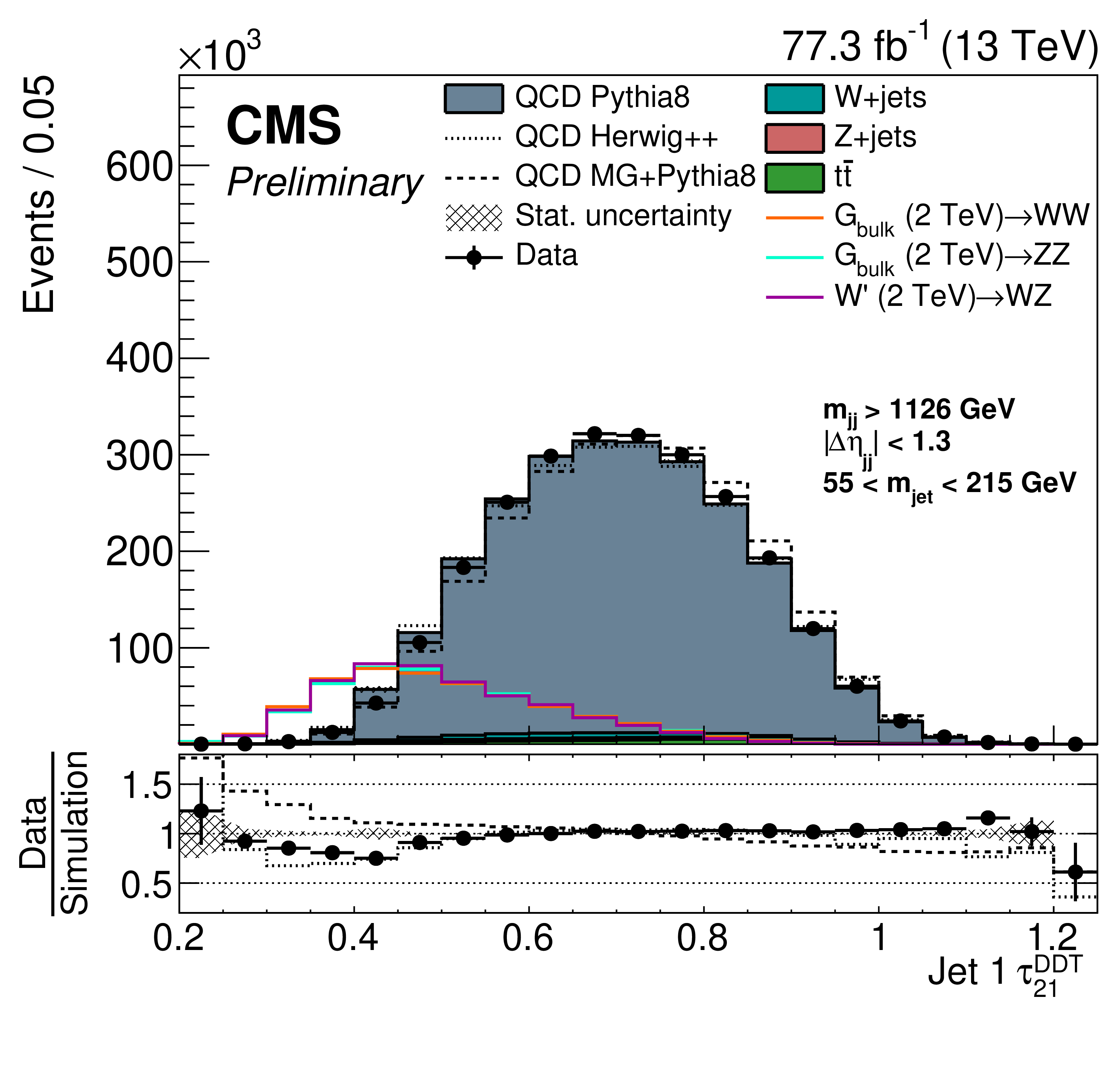
Figure 3-b:
${\tau _{21}^\textbf {DDT}}$ distribution for randomly sorted selected jets for events with a jet mass between 55 and 215 GeV in data and simulation. For the QCD multijet simulation, several alternative predictions are shown, scaled to the data minus the other background processes, which are scaled to their SM expectation as described in the text. The different signal distributions are arbitrarily scaled for visibility. No selection on ${\tau _{21}^\textbf {DDT}}$ is applied. |
png pdf |
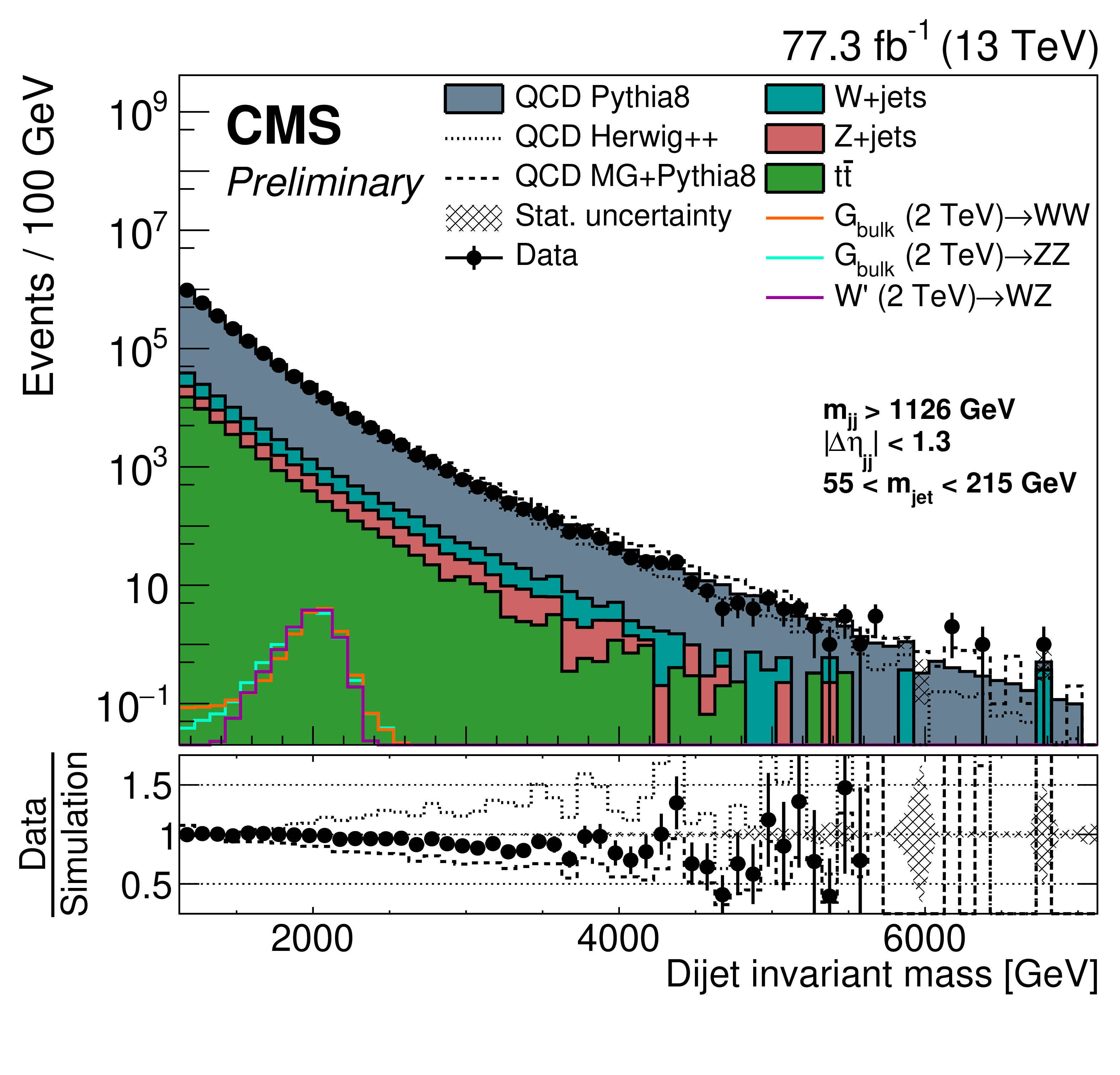
Figure 3-c:
Dijet invariant mass distribution for events with a jet mass between 55 and 215 GeV in data and simulation. For the QCD multijet simulation, several alternative predictions are shown, scaled to the data minus the other background processes, which are scaled to their SM expectation as described in the text. The different signal distributions are arbitrarily scaled for visibility. No selection on ${\tau _{21}^\textbf {DDT}}$ is applied. |
png pdf |
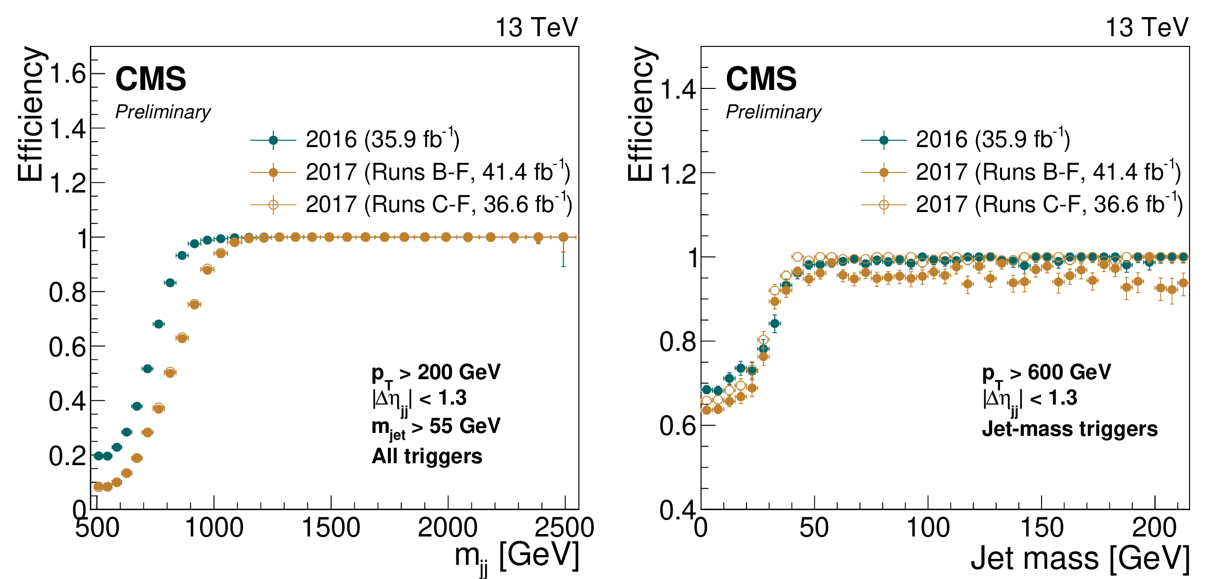
Figure 4:
Left: trigger efficiency as a function of the dijet invariant mass using a combination of all analysis triggers. Right: trigger efficiency as a function of the jet mass for triggers requiring an online trimmed mass of at least 30 GeV. The solid yellow markers correspond to the trigger efficiencies for the full 2017 data set and do not reach 100% efficiency due to the jet-mass based triggers being unavailable during a period of data taking (Run B, corresponding to 4.8 fb$^{-1}$). The hollow yellow markers are the corresponding efficiencies excluding this period. Uncertainties shown are statistical only. |
png pdf |
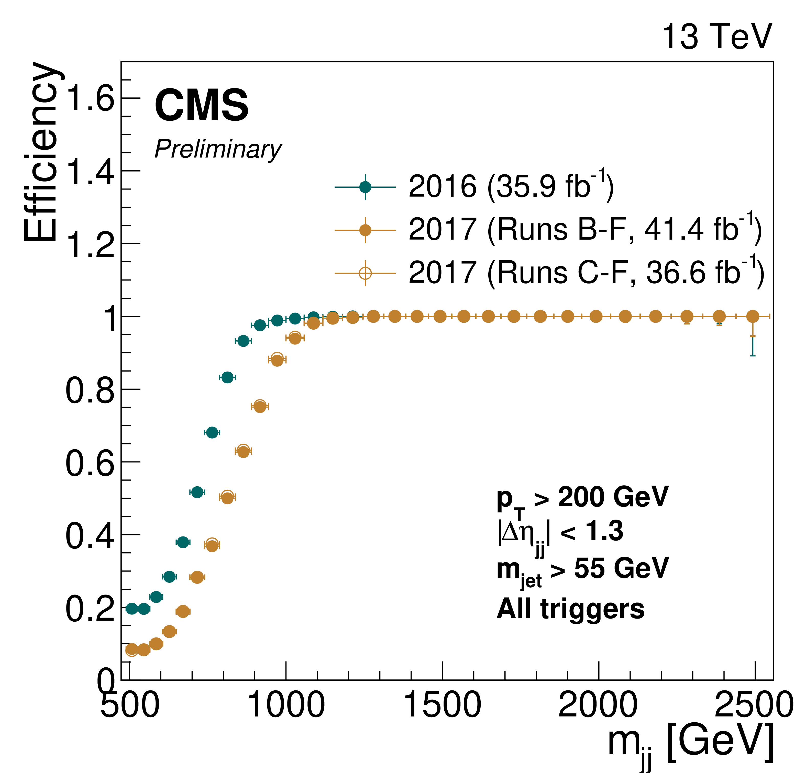
Figure 4-a:
Trigger efficiency as a function of the dijet invariant mass using a combination of all analysis triggers. The solid yellow markers correspond to the trigger efficiencies for the full 2017 data set and do not reach 100% efficiency due to the jet-mass based triggers being unavailable during a period of data taking (Run B, corresponding to 4.8 fb$^{-1}$). The hollow yellow markers are the corresponding efficiencies excluding this period. Uncertainties shown are statistical only. |
png pdf |
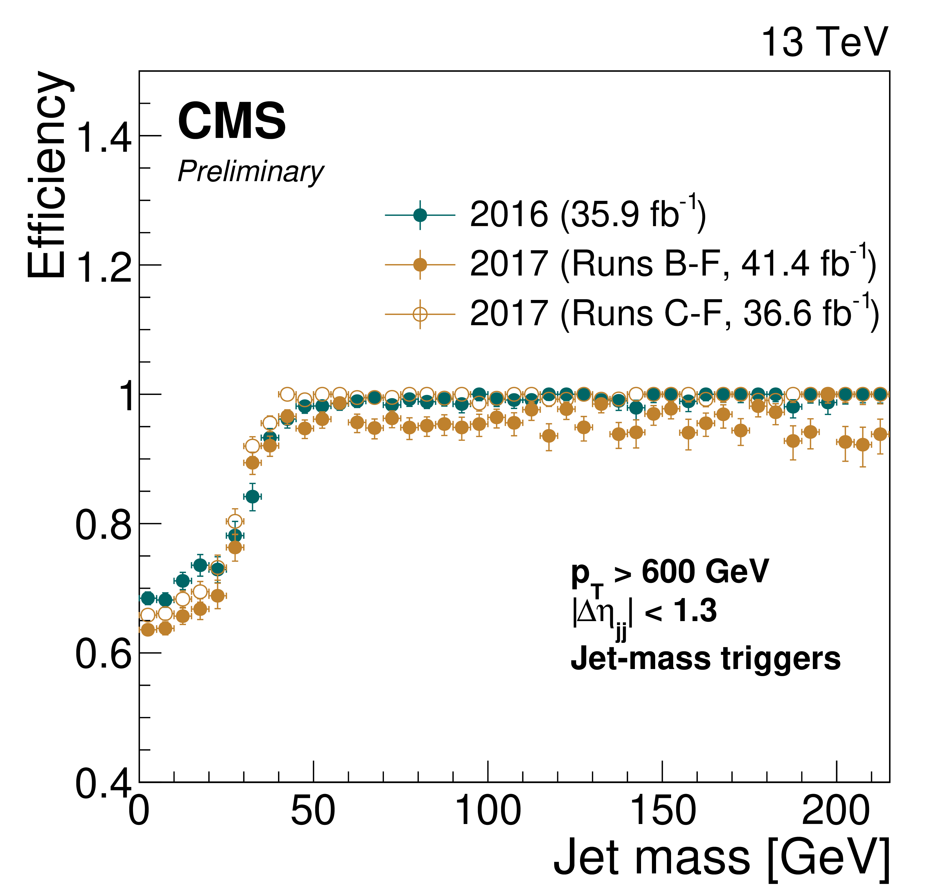
Figure 4-b:
Trigger efficiency as a function of the jet mass for triggers requiring an online trimmed mass of at least 30 GeV. The solid yellow markers correspond to the trigger efficiencies for the full 2017 data set and do not reach 100% efficiency due to the jet-mass based triggers being unavailable during a period of data taking (Run B, corresponding to 4.8 fb$^{-1}$). The hollow yellow markers are the corresponding efficiencies excluding this period. Uncertainties shown are statistical only. |
png pdf |
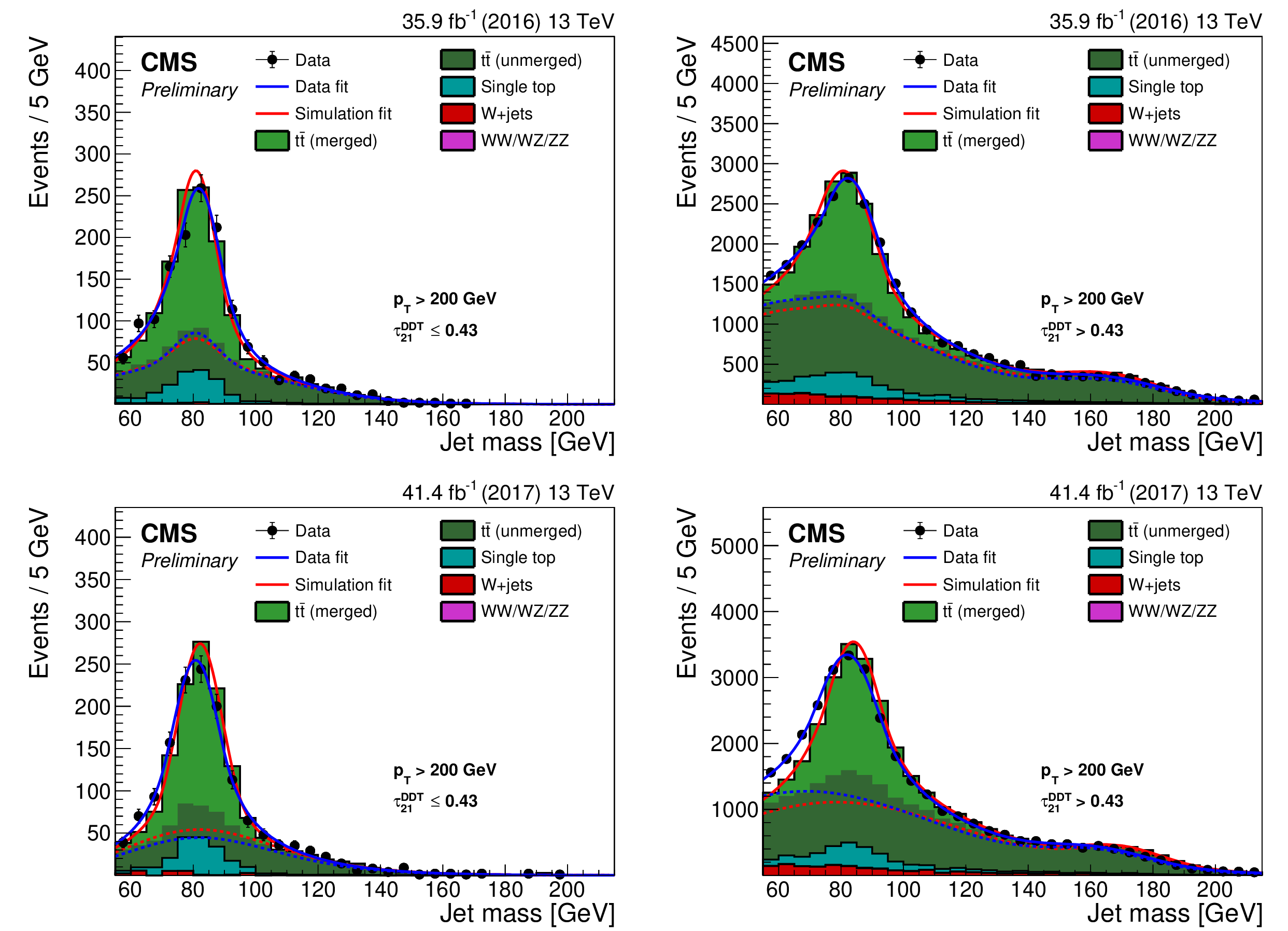
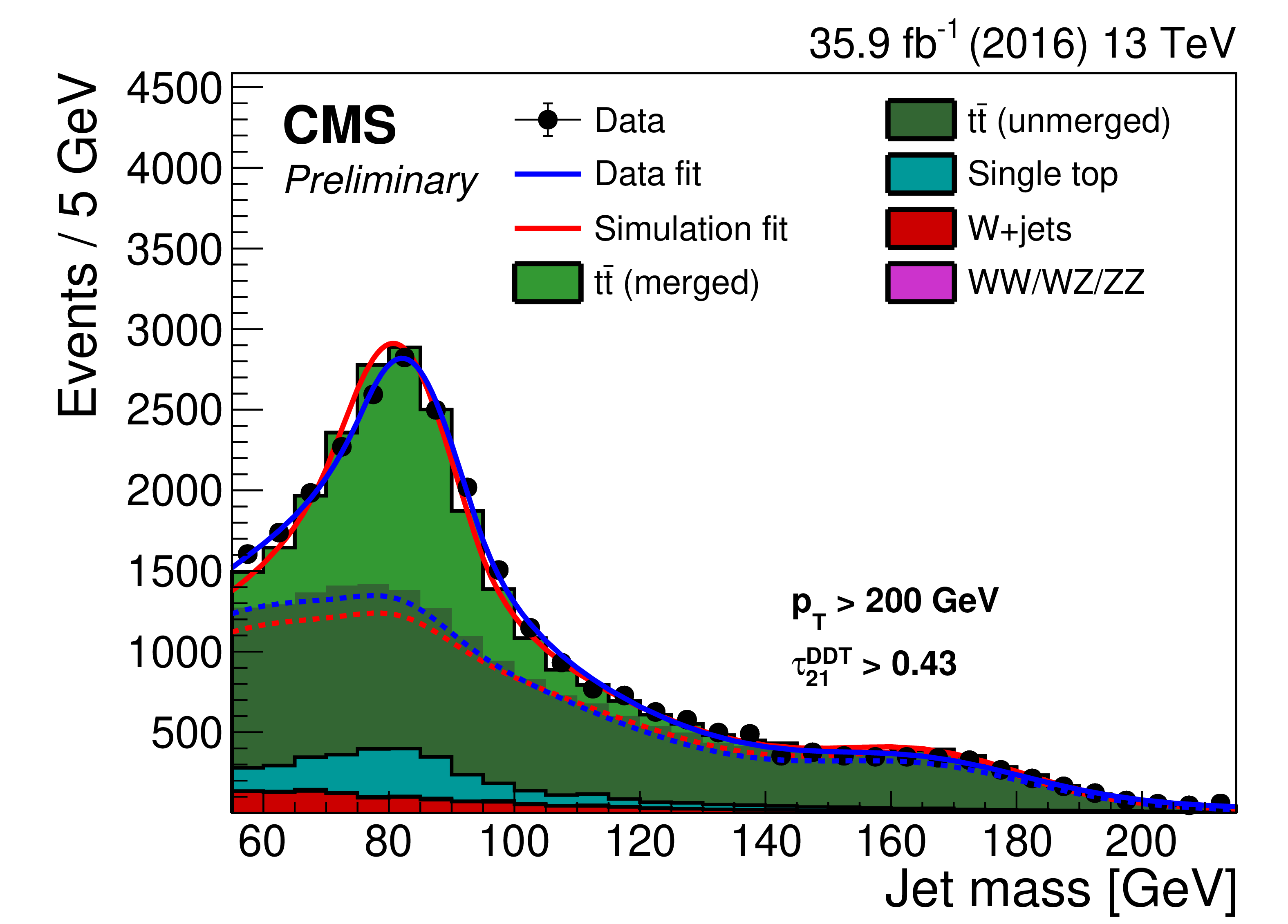
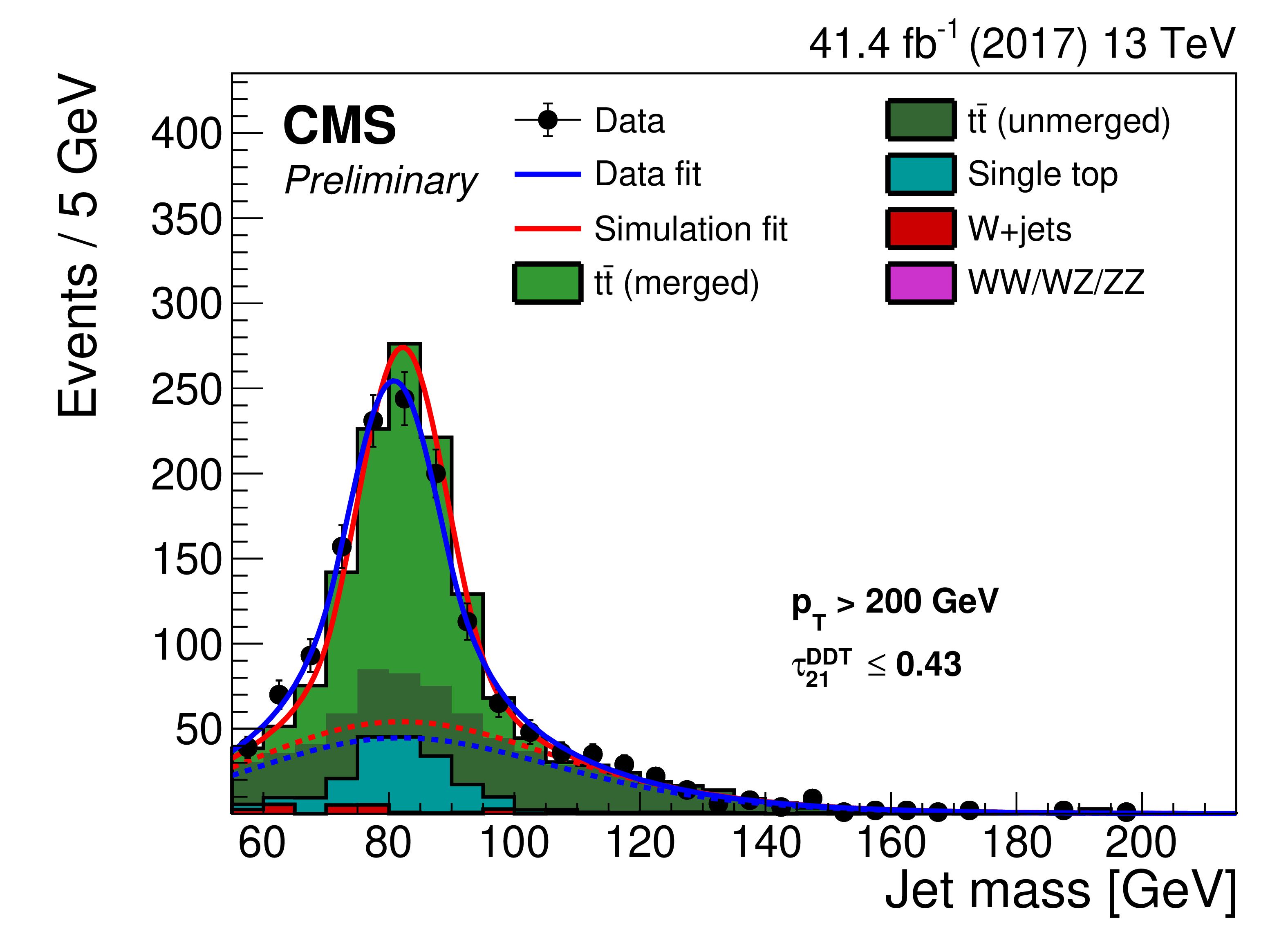
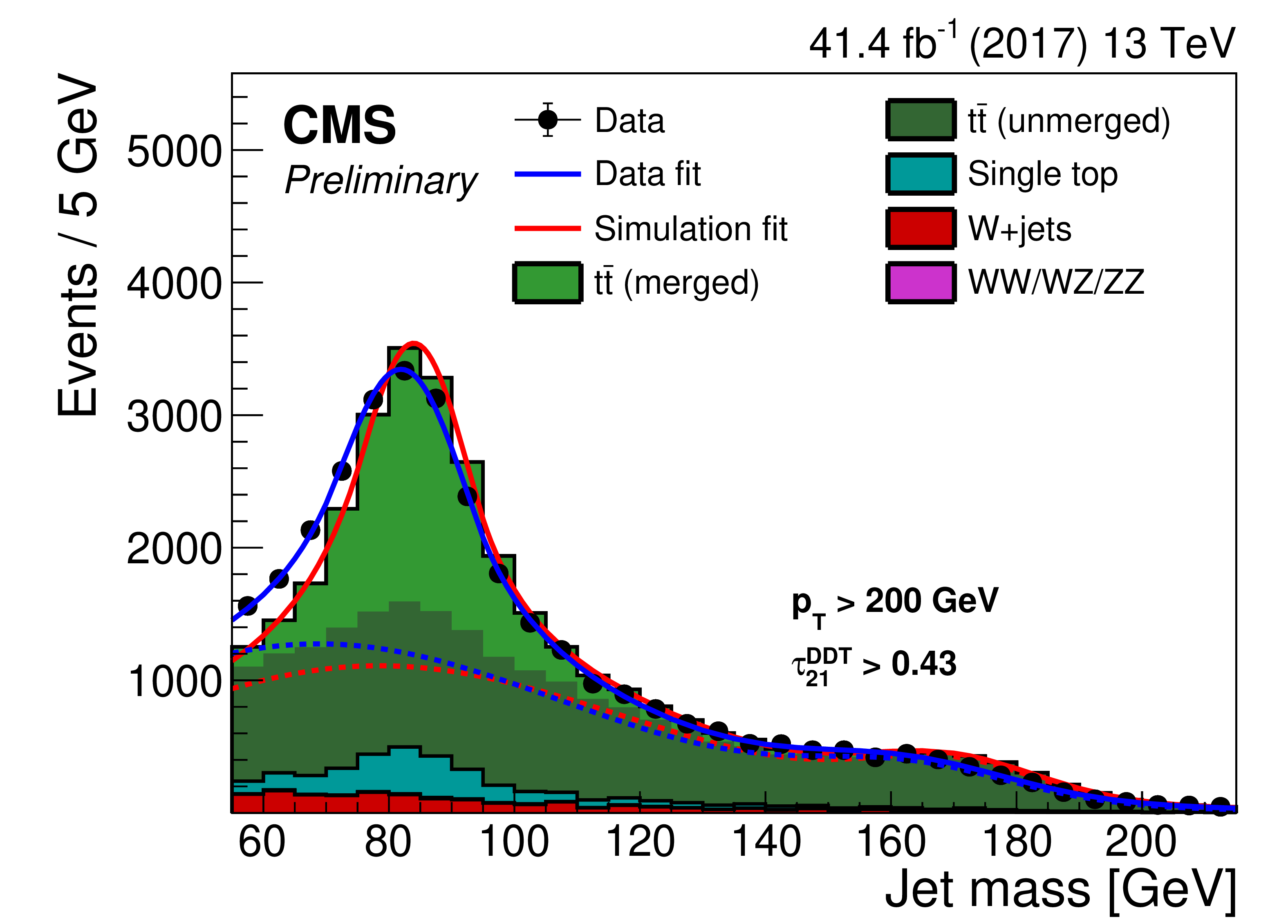
Figure 5:
Jet mass distribution for events that pass (left) and fail (right) the $ {\tau _{21}^\textbf {DDT}} < $ 0.43 selection in the ${{\mathrm {t}\overline {\mathrm {t}}}}$ control sample. The result of the fit to data and simulation is shown by the solid blue and solid red lines, respectively. The background components of the fit are shown as dashed-dotted lines. The fit to 2016 data is shown in the upper panels and the fit to 2017 data in the lower panels. |

png pdf |
Figure 5-a:
Jet mass distribution for events that pass the $ {\tau _{21}^\textbf {DDT}} < $ 0.43 selection in the ${{\mathrm {t}\overline {\mathrm {t}}}}$ control sample. The result of the fit to data and simulation is shown by the solid blue and solid red lines, respectively. The background components of the fit are shown as dashed-dotted lines. The fit to 2016 data is shown. |
png pdf |
Figure 5-b:
Jet mass distribution for events that fail the $ {\tau _{21}^\textbf {DDT}} < $ 0.43 selection in the ${{\mathrm {t}\overline {\mathrm {t}}}}$ control sample. The result of the fit to data and simulation is shown by the solid blue and solid red lines, respectively. The background components of the fit are shown as dashed-dotted lines. The fit to 2016 data is shown. |
png pdf |
Figure 5-c:
Jet mass distribution for events that pass the $ {\tau _{21}^\textbf {DDT}} < $ 0.43 selection in the ${{\mathrm {t}\overline {\mathrm {t}}}}$ control sample. The result of the fit to data and simulation is shown by the solid blue and solid red lines, respectively. The background components of the fit are shown as dashed-dotted lines. The fit to 2017 data is shown. |
png pdf |
Figure 5-d:
Jet mass distribution for events that fail the $ {\tau _{21}^\textbf {DDT}} < $ 0.43 selection in the ${{\mathrm {t}\overline {\mathrm {t}}}}$ control sample. The result of the fit to data and simulation is shown by the solid blue and solid red lines, respectively. The background components of the fit are shown as dashed-dotted lines. The fit to 2017 data is shown. |
png pdf |
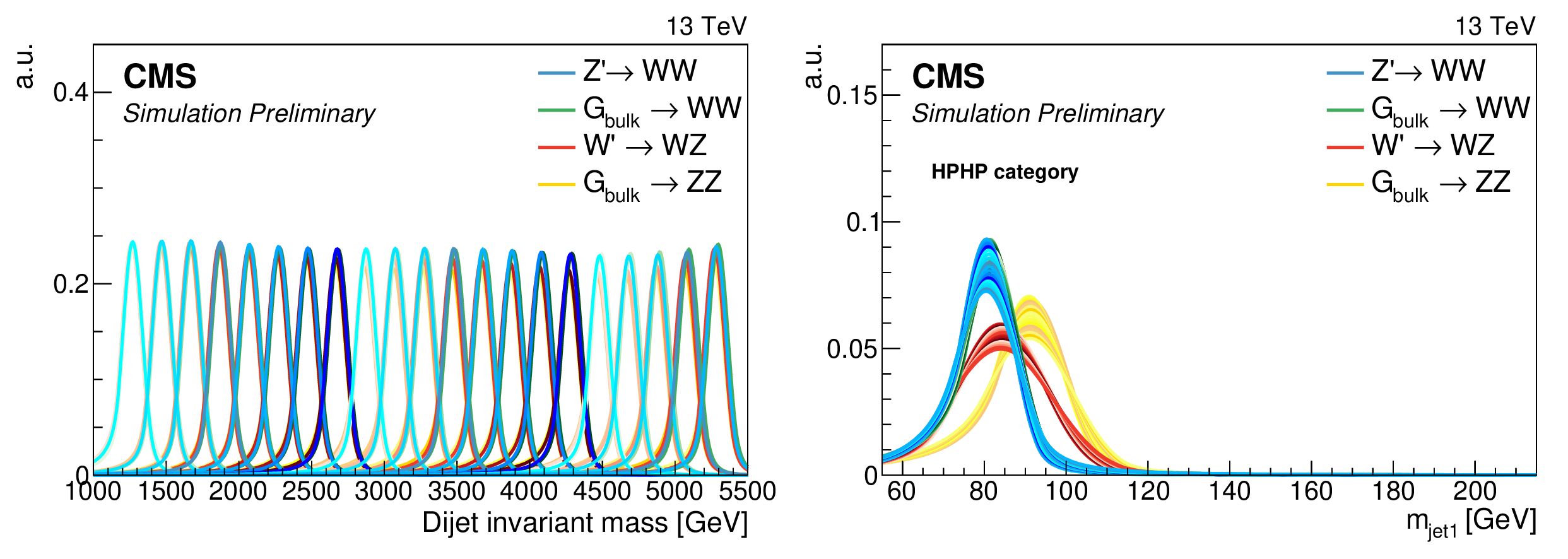
Figure 6:
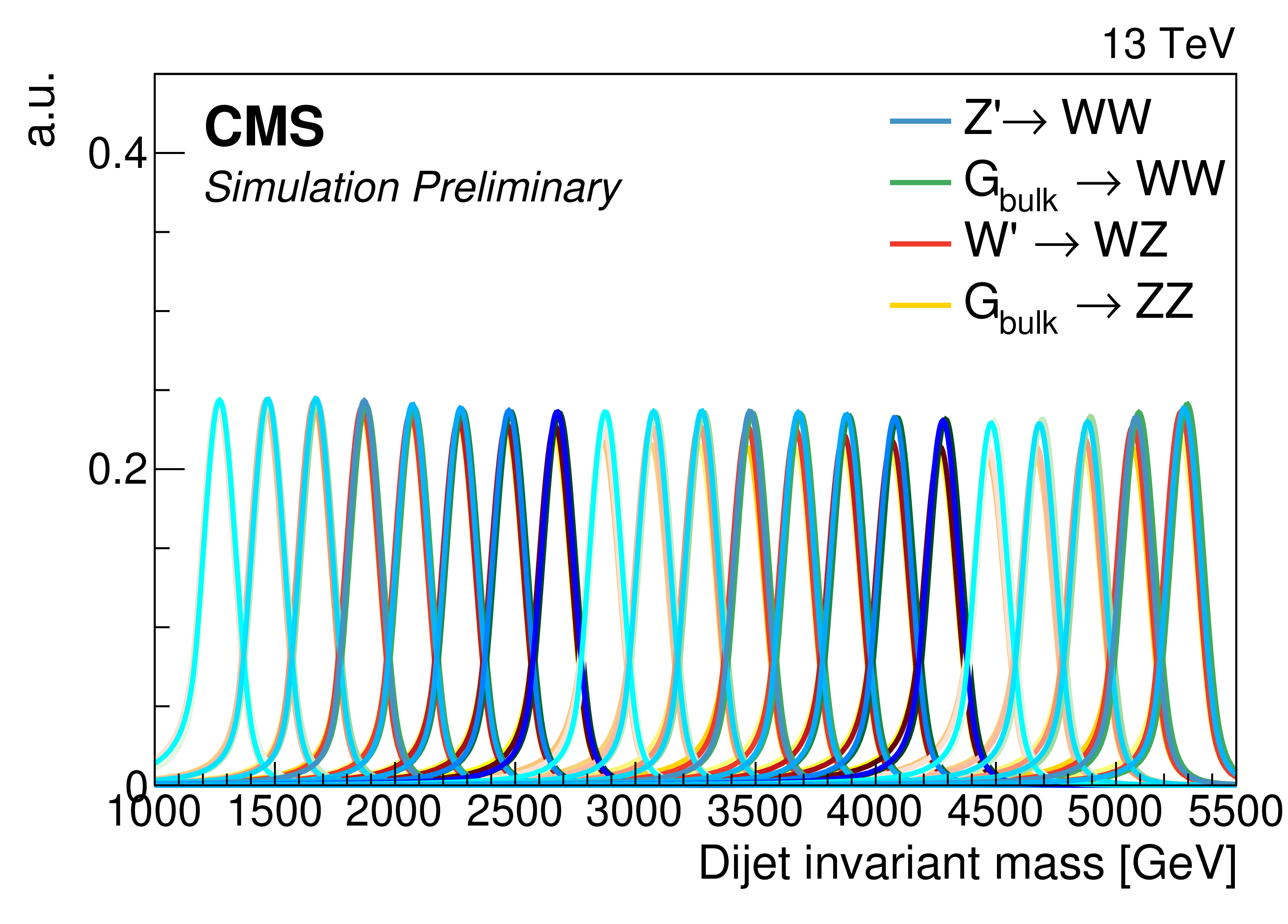
Final $ {m_\mathrm {VV}} $ (left) and ${m_\text {jet2}}$ (right) signal shapes extracted from the parametrisation. Shown here is a $ {{\mathrm {G}} _{\text {bulk}}} $ decaying to WW. The ${m_\text {jet2}}$ distribution is for a jet in the HPHP category. |
png pdf |
Figure 6-a:
Final $ {m_\mathrm {VV}} $ signal shape extracted from the parametrisation. Shown here is a $ {{\mathrm {G}} _{\text {bulk}}} $ decaying to WW. The ${m_\text {jet2}}$ distribution is for a jet in the HPHP category. |

png pdf |
Figure 6-b:
Final ${m_\text {jet2}}$ signal shape extracted from the parametrisation. Shown here is a $ {{\mathrm {G}} _{\text {bulk}}} $ decaying to WW. The ${m_\text {jet2}}$ distribution is for a jet in the HPHP category. |
png pdf |
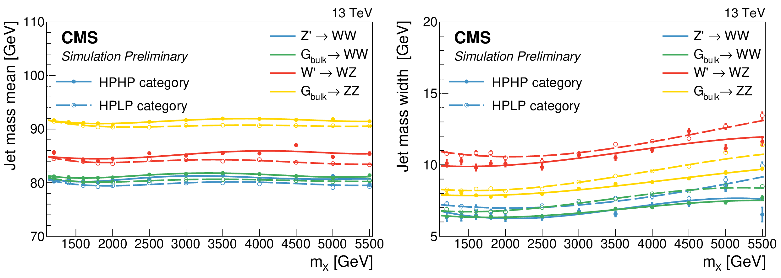
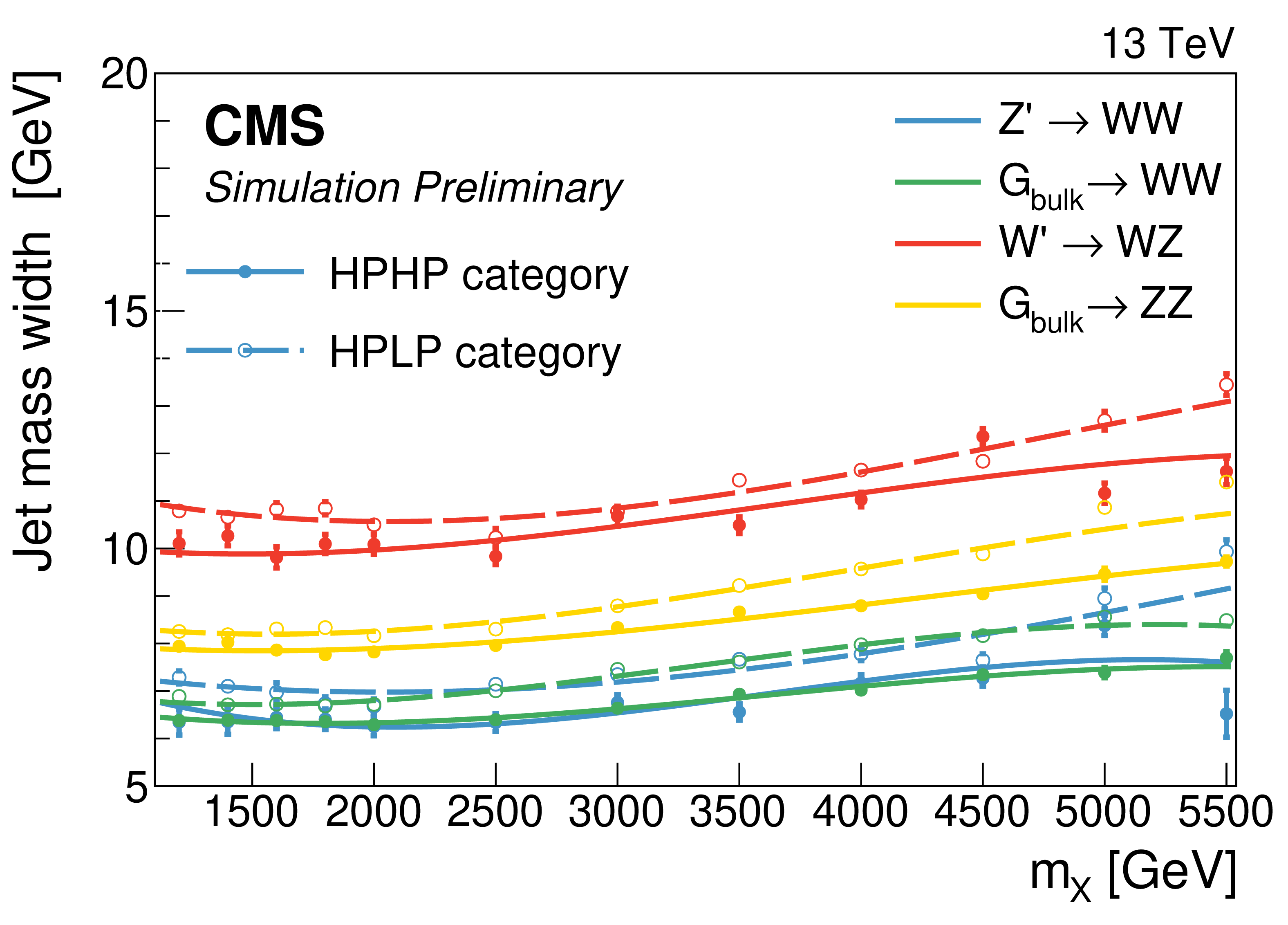
Figure 7:
The mass scale (left) and resolution (right) of the jet as a function of $m_\mathrm {X}$, obtained from the mean and $\sigma $ of the Crystal ball function used to fit the jet mass spectrum. |

png pdf |
Figure 7-a:
The mass scale of the jet as a function of $m_\mathrm {X}$, obtained from the mean and $\sigma $ of the Crystal ball function used to fit the jet mass spectrum. |
png pdf |
Figure 7-b:
The resolution of the jet as a function of $m_\mathrm {X}$, obtained from the mean and $\sigma $ of the Crystal ball function used to fit the jet mass spectrum. |
png pdf |
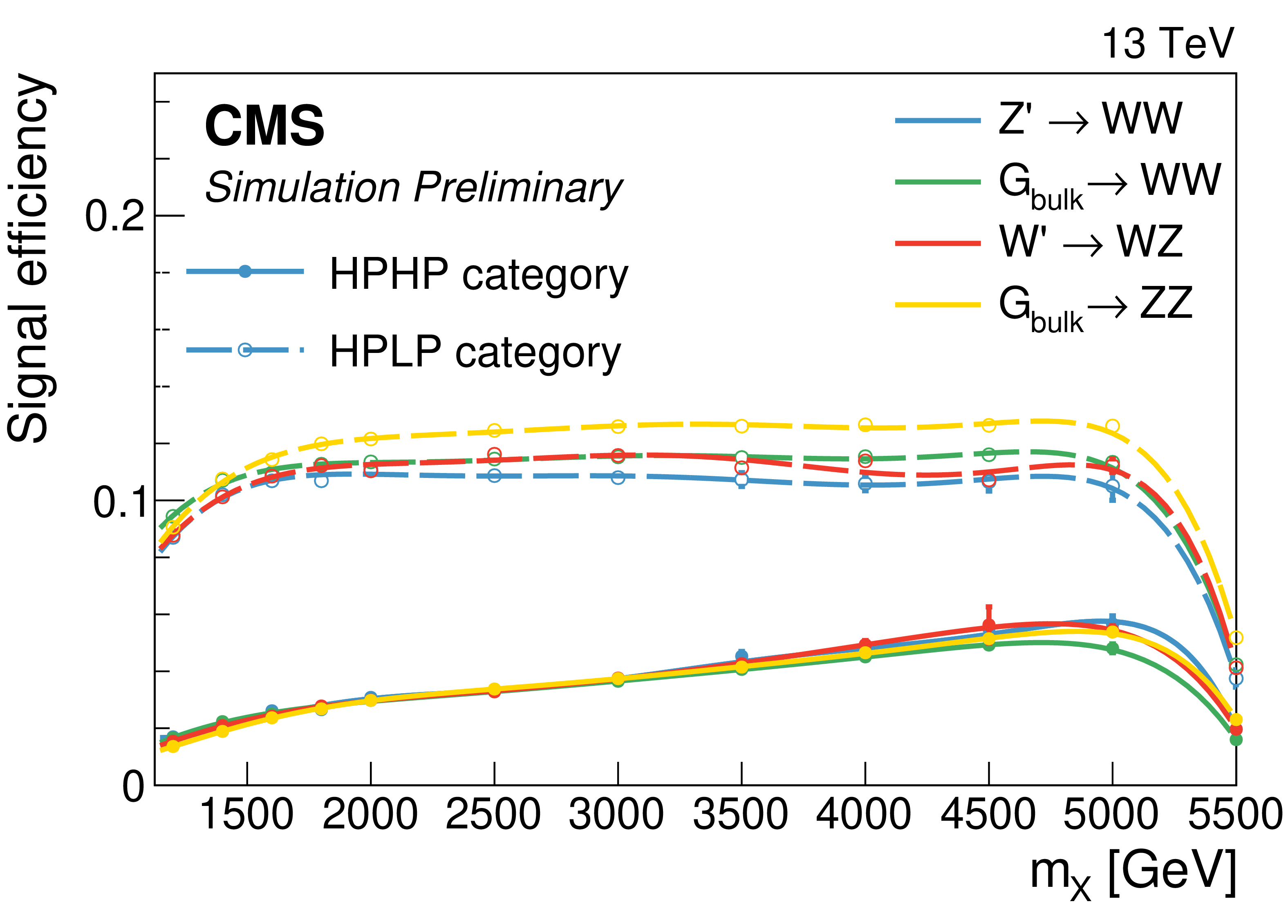
Figure 8:
Total signal efficiency after all selections are applied as a function of $m_\mathrm {X}$ for signal models with a $ {{\mathrm {G}} _{\text {bulk}}} $ decaying to WW, $ {{\mathrm {G}} _{\text {bulk}}} $ decaying to ZZ, and W' decaying to WZ. The denominator is the number of generated events. The solid and dashed lines show the signal efficiencies for the HPHP and HPLP categories, respectively. |
png pdf |
Figure 9:
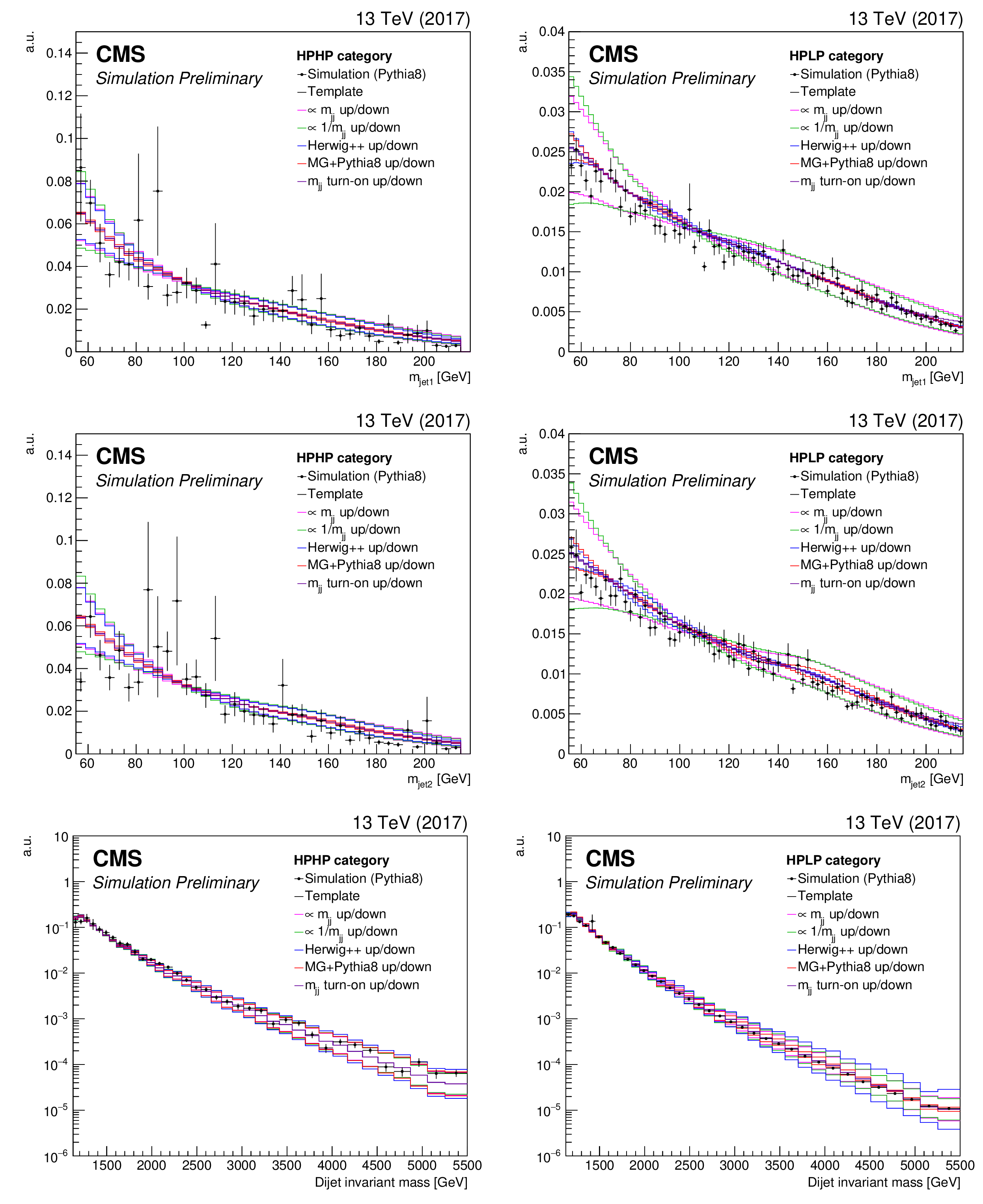
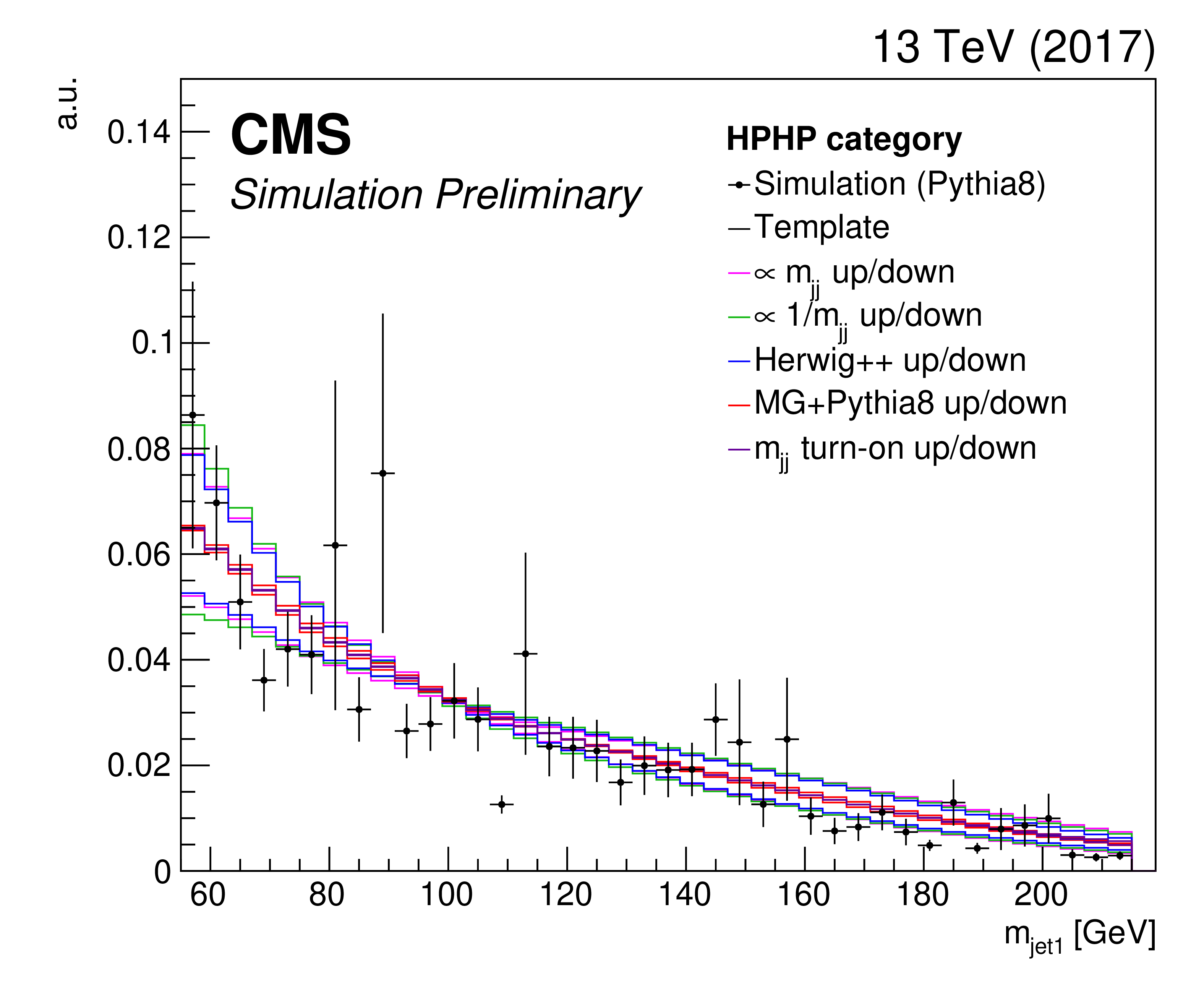
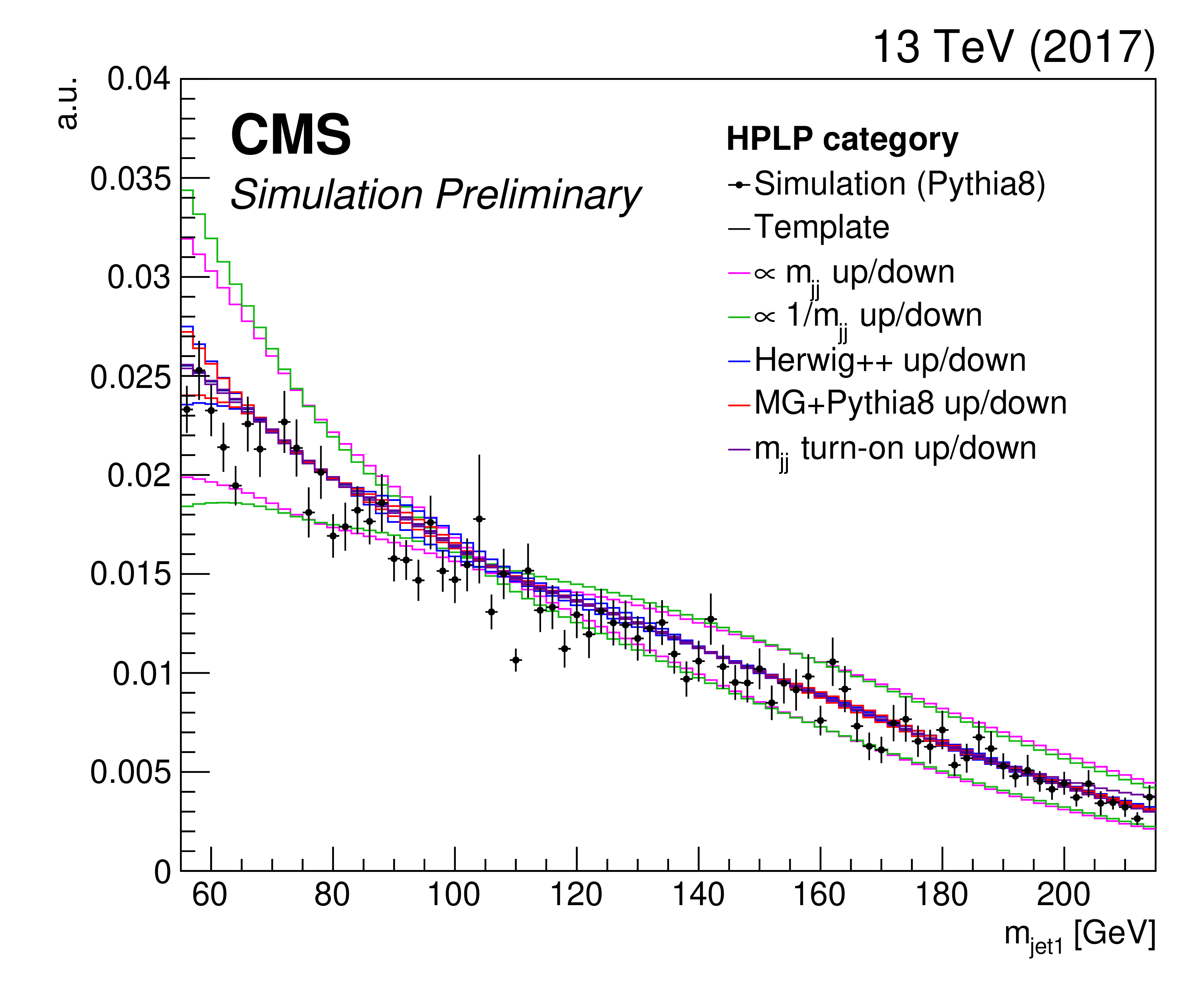
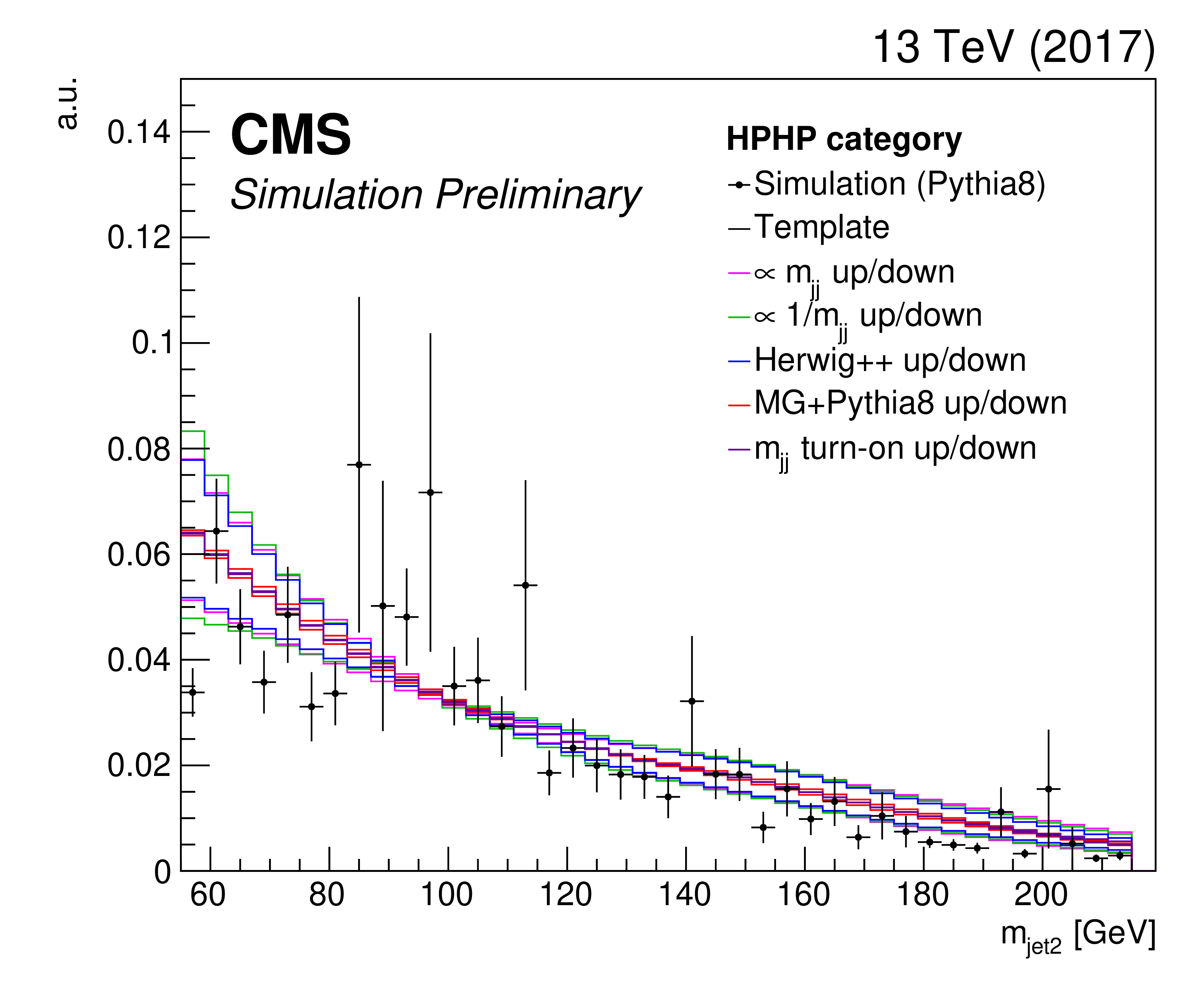
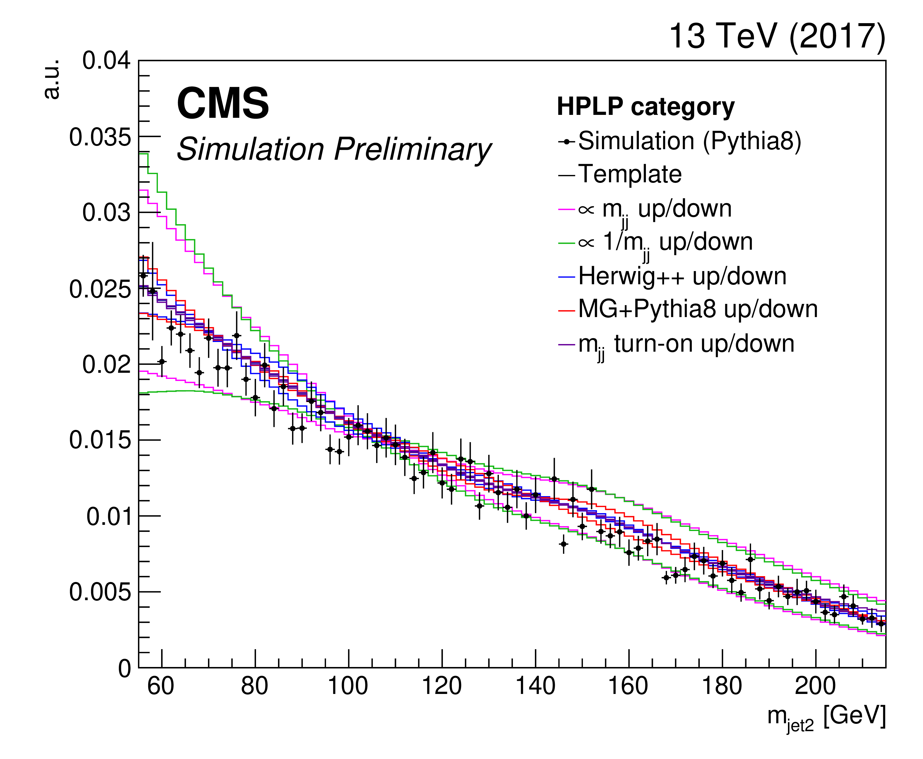
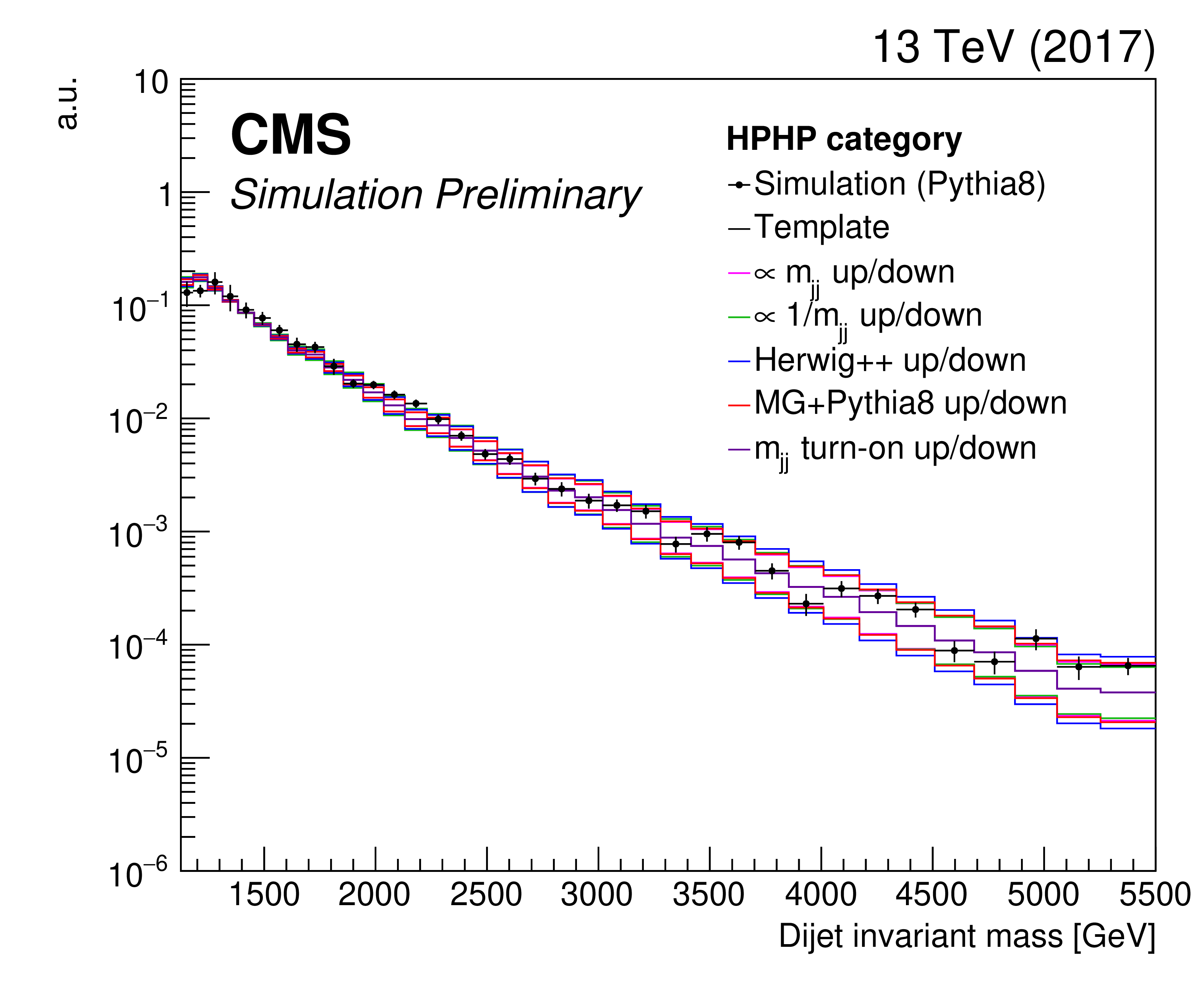
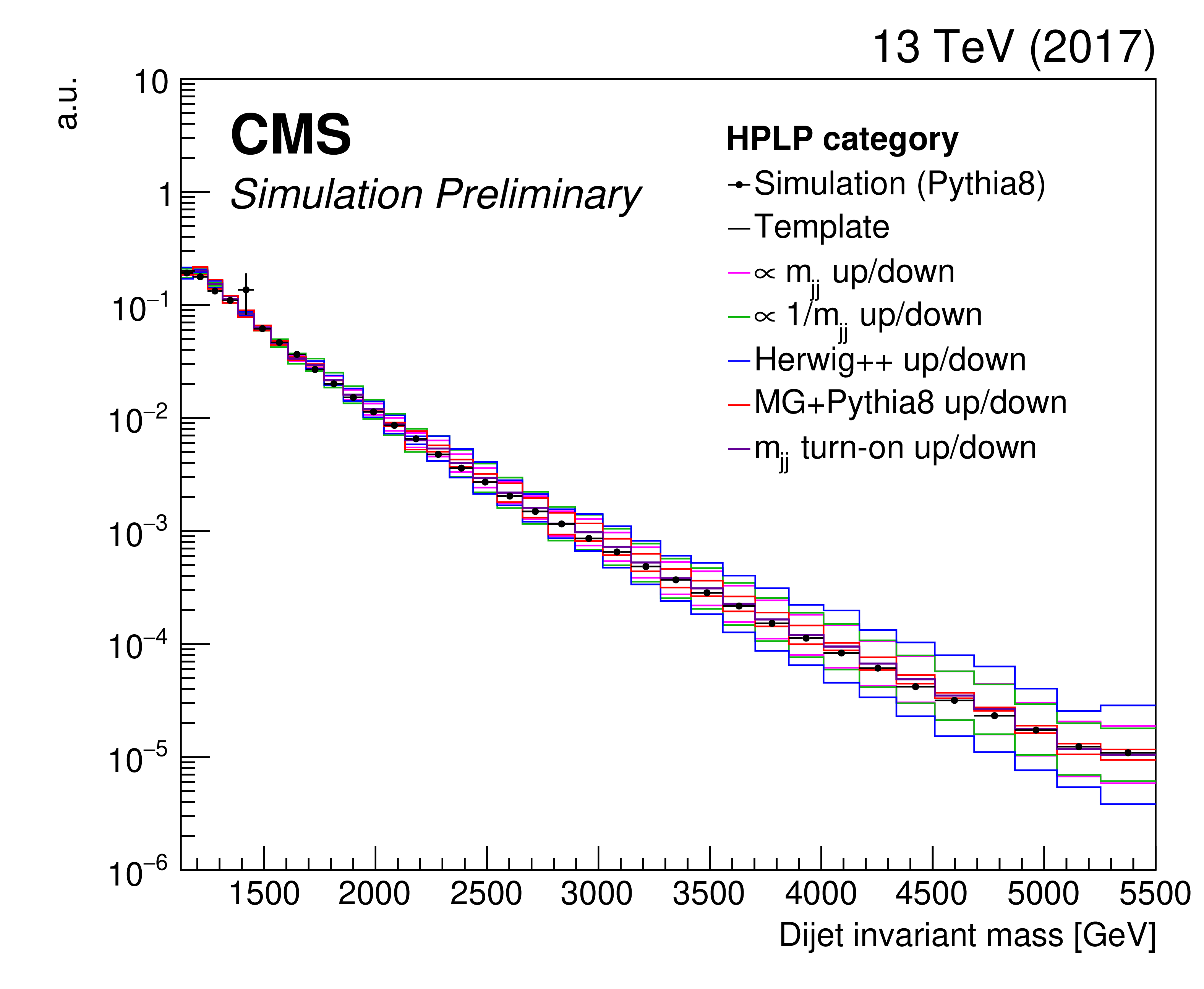
Nominal QCD multijet simulation using PYTHIA 8 (markers) and derived kernel using a forward-folding kernel approach (black solid line), shown together with the five alternate shapes that are added to the fit as shape nuisance parameters. The shapes for the high purity category (left) and low purity category (right) obtained with the 2017 simulation are shown. |
png pdf |
Figure 9-a:
Nominal QCD multijet simulation using PYTHIA 8 (markers) and derived kernel using a forward-folding kernel approach (black solid line), shown together with the five alternate shapes that are added to the fit as shape nuisance parameters. The shape for the high purity category obtained with the 2017 simulation is shown. |
png pdf |
Figure 9-b:
Nominal QCD multijet simulation using PYTHIA 8 (markers) and derived kernel using a forward-folding kernel approach (black solid line), shown together with the five alternate shapes that are added to the fit as shape nuisance parameters. The shape for the low purity category obtained with the 2017 simulation is shown. |
png pdf |
Figure 9-c:
Nominal QCD multijet simulation using PYTHIA 8 (markers) and derived kernel using a forward-folding kernel approach (black solid line), shown together with the five alternate shapes that are added to the fit as shape nuisance parameters. The shape for the high purity category obtained with the 2017 simulation is shown. |
png pdf |
Figure 9-d:
Nominal QCD multijet simulation using PYTHIA 8 (markers) and derived kernel using a forward-folding kernel approach (black solid line), shown together with the five alternate shapes that are added to the fit as shape nuisance parameters. The shape for the low purity category obtained with the 2017 simulation is shown. |
png pdf |
Figure 9-e:
Nominal QCD multijet simulation using PYTHIA 8 (markers) and derived kernel using a forward-folding kernel approach (black solid line), shown together with the five alternate shapes that are added to the fit as shape nuisance parameters. The shape for the high purity category obtained with the 2017 simulation is shown. |
png pdf |
Figure 9-f:
Nominal QCD multijet simulation using PYTHIA 8 (markers) and derived kernel using a forward-folding kernel approach (black solid line), shown together with the five alternate shapes that are added to the fit as shape nuisance parameters. The shape for the low purity category obtained with the 2017 simulation is shown. |
png pdf |
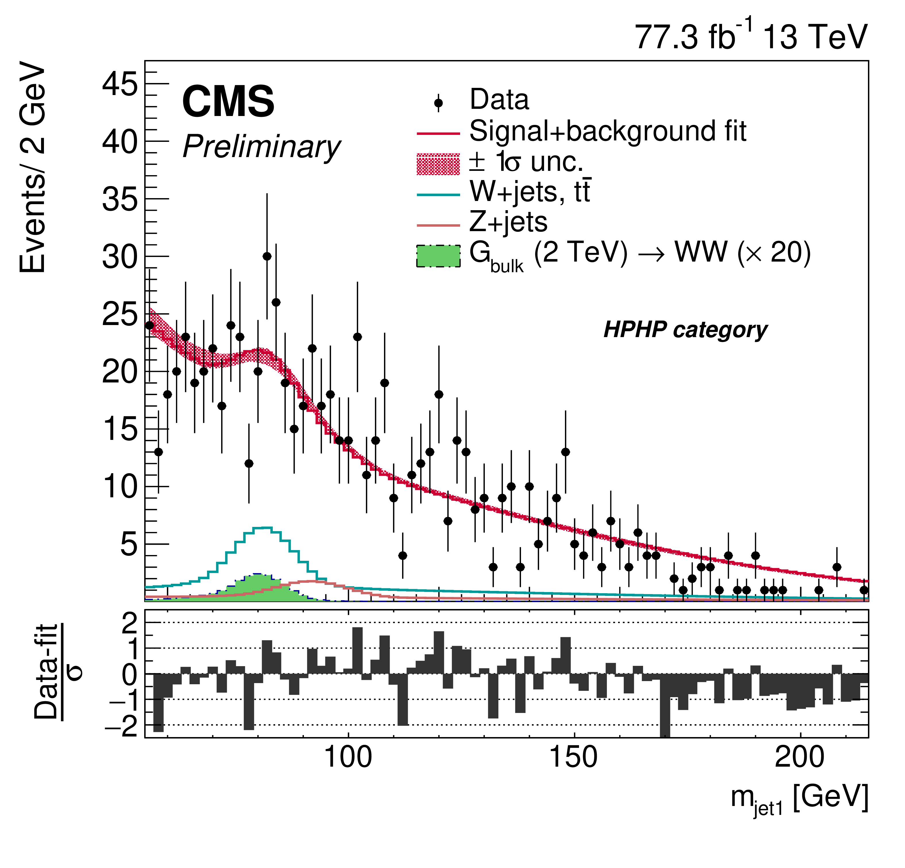
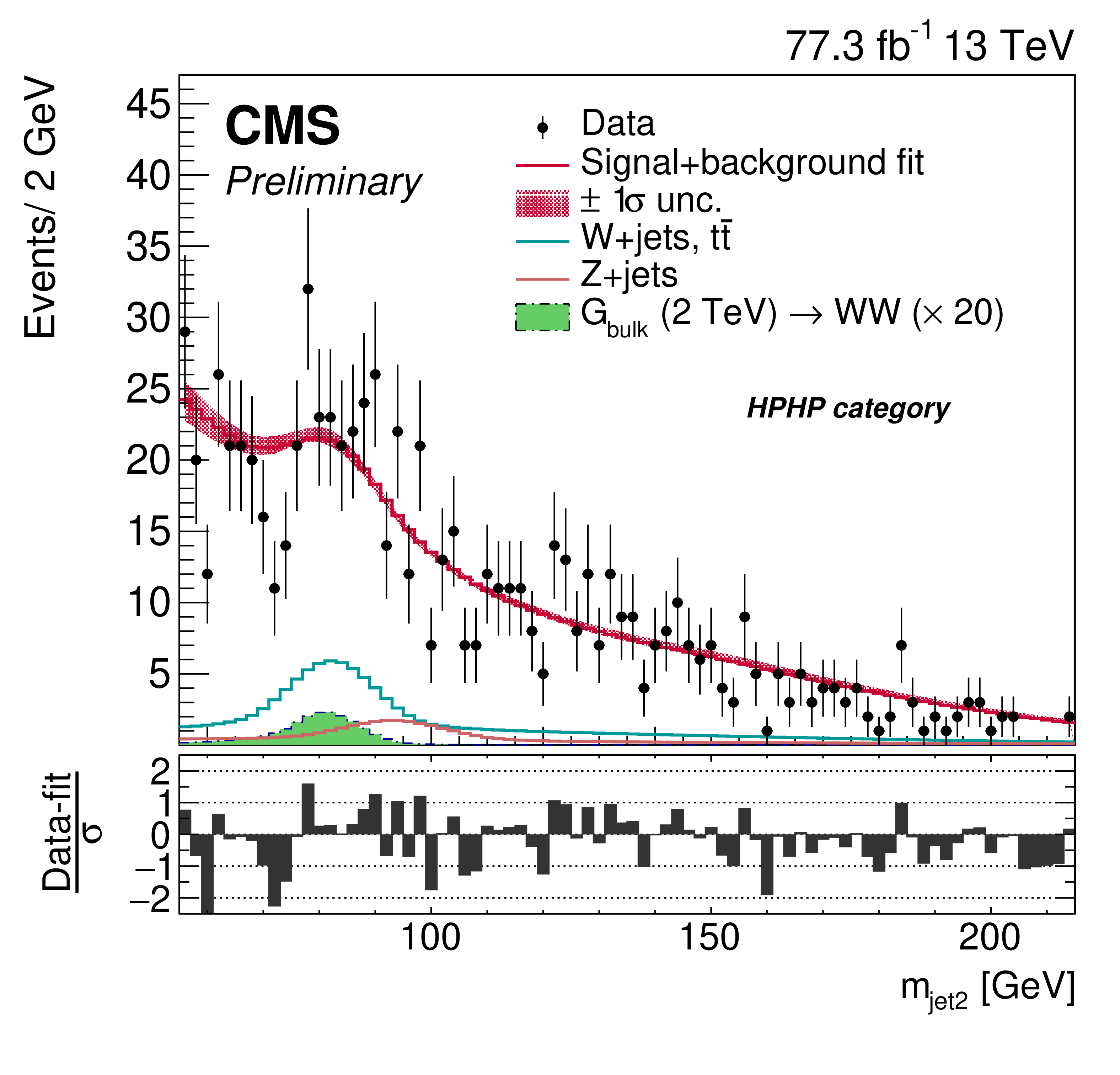
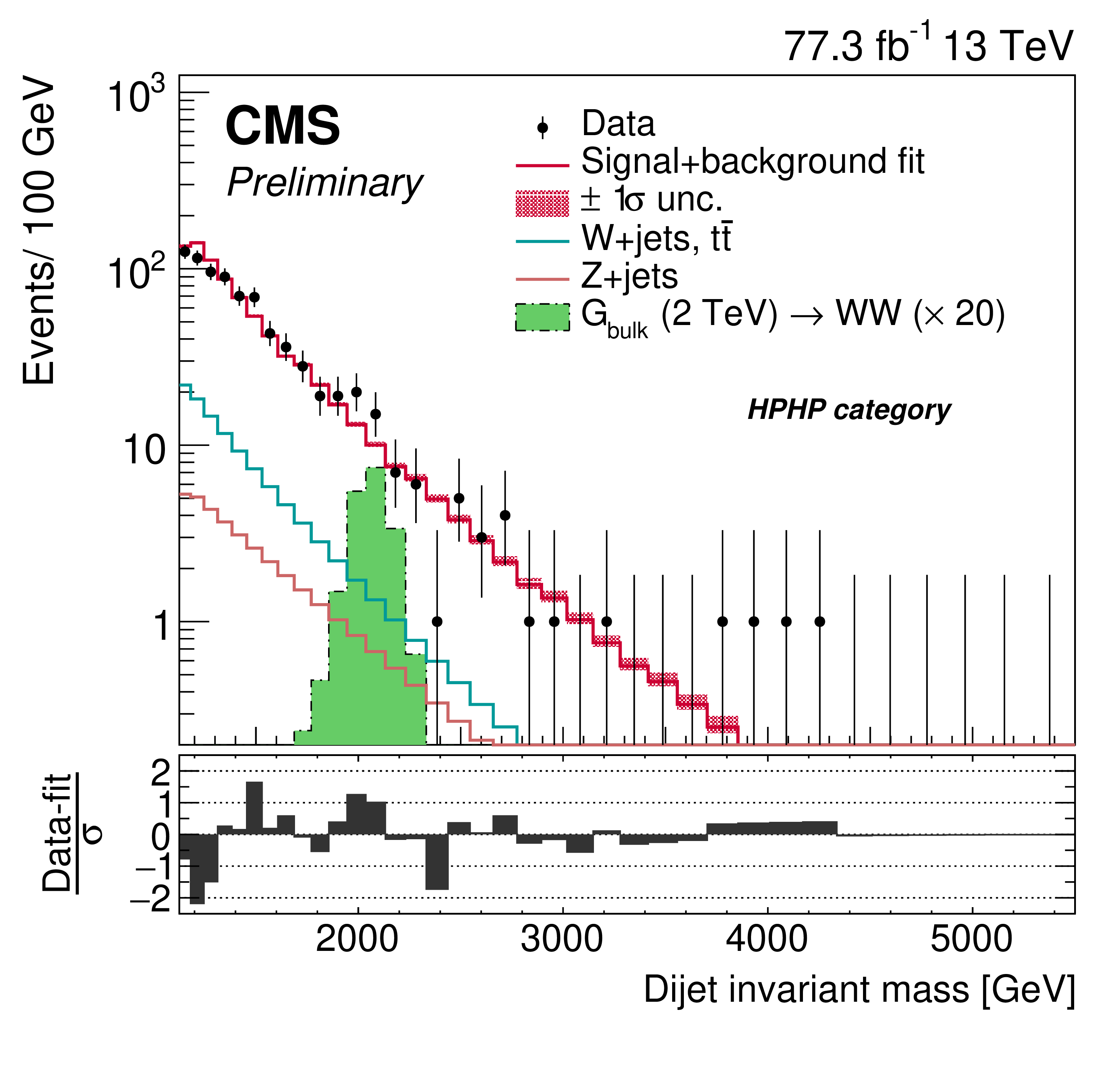
Figure 10:
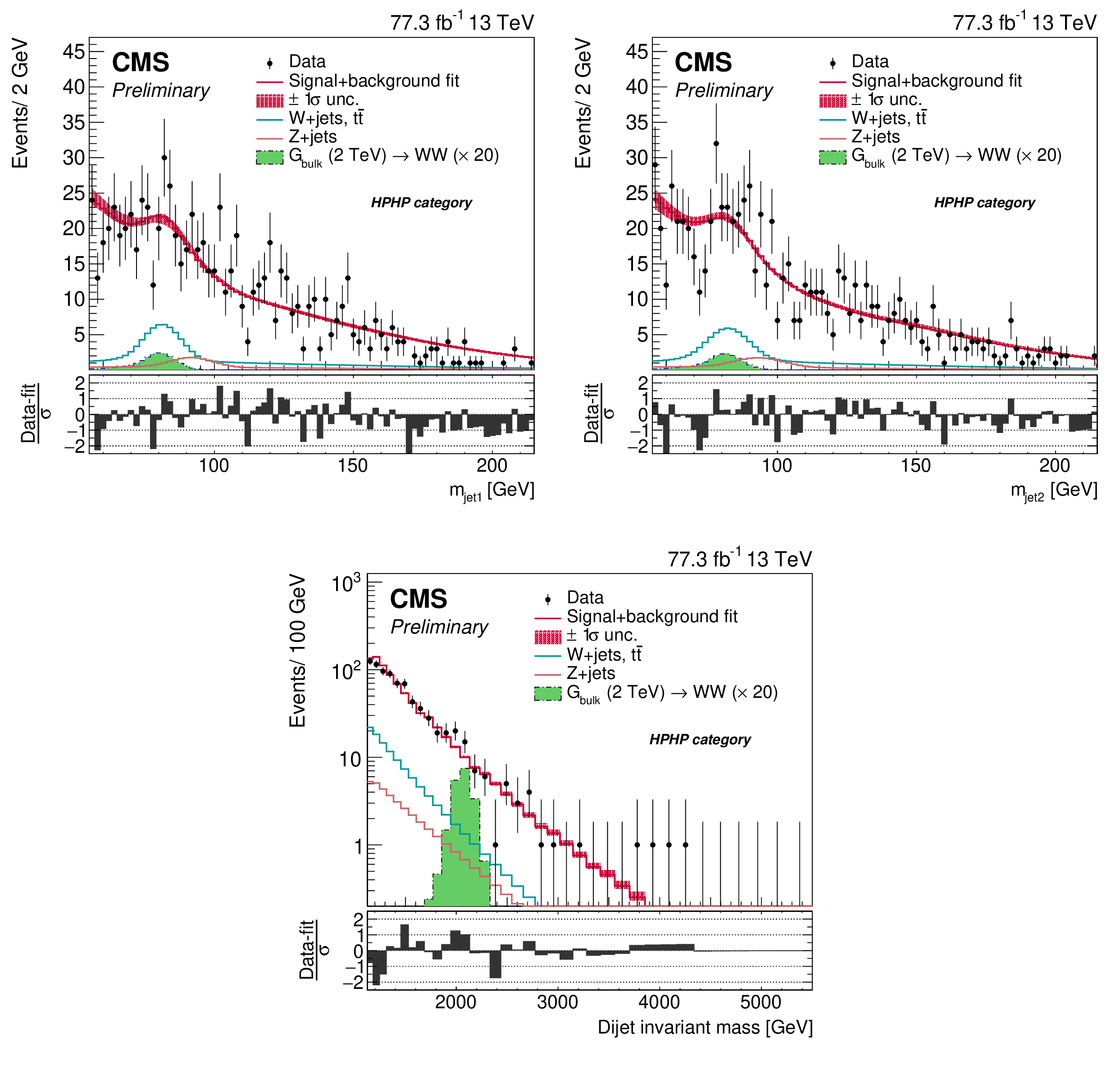
Comparison between the fitted result and data distributions of ${m_\text {jet1}}$ (left), ${m_\text {jet2}}$ (middle), and ${m_\mathrm {VV}}$ (right) in the HPHP category. The background shape uncertainty is shown as a red shaded band, and the statistical uncertainties of the data are shown as vertical bars. An example of a signal distribution is overlaid, using an arbitrary normalisation. The corresponding pull distributions (Data-fit)/$\sigma $, where $\sigma = \sqrt {\sigma _\mathrm {data}^2 - \sigma _\mathrm {fit}^2}$ for a bin in ${m_\mathrm {VV}}$ to ensure a Gaussian pull-distribution as defined in [78], are shown below each ${m_\mathrm {VV}}$ plot. |
png pdf |
Figure 10-a:
Comparison between the fitted result and data distributions of ${m_\text {jet1}}$ in the HPHP category. The background shape uncertainty is shown as a red shaded band, and the statistical uncertainties of the data are shown as vertical bars. An example of a signal distribution is overlaid, using an arbitrary normalisation. The corresponding pull distributions (Data-fit)/$\sigma $, where $\sigma = \sqrt {\sigma _\mathrm {data}^2 - \sigma _\mathrm {fit}^2}$ for a bin in ${m_\mathrm {VV}}$ to ensure a Gaussian pull-distribution as defined in [78], are shown below the ${m_\mathrm {VV}}$ plot. |
png pdf |
Figure 10-b:
Comparison between the fitted result and data distributions of ${m_\text {jet2}}$ in the HPHP category. The background shape uncertainty is shown as a red shaded band, and the statistical uncertainties of the data are shown as vertical bars. An example of a signal distribution is overlaid, using an arbitrary normalisation. The corresponding pull distributions (Data-fit)/$\sigma $, where $\sigma = \sqrt {\sigma _\mathrm {data}^2 - \sigma _\mathrm {fit}^2}$ for a bin in ${m_\mathrm {VV}}$ to ensure a Gaussian pull-distribution as defined in [78], are shown below the ${m_\mathrm {VV}}$ plot. |
png pdf |
Figure 10-c:
Comparison between the fitted result and data distributions of ${m_\mathrm {VV}}$ in the HPHP category. The background shape uncertainty is shown as a red shaded band, and the statistical uncertainties of the data are shown as vertical bars. An example of a signal distribution is overlaid, using an arbitrary normalisation. The corresponding pull distributions (Data-fit)/$\sigma $, where $\sigma = \sqrt {\sigma _\mathrm {data}^2 - \sigma _\mathrm {fit}^2}$ for a bin in ${m_\mathrm {VV}}$ to ensure a Gaussian pull-distribution as defined in [78], are shown below the ${m_\mathrm {VV}}$ plot. |
png pdf |
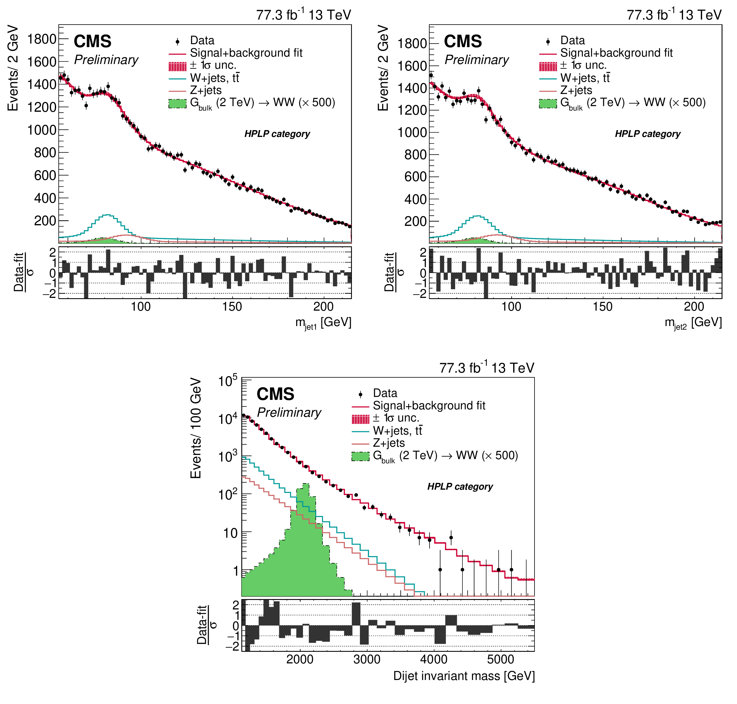
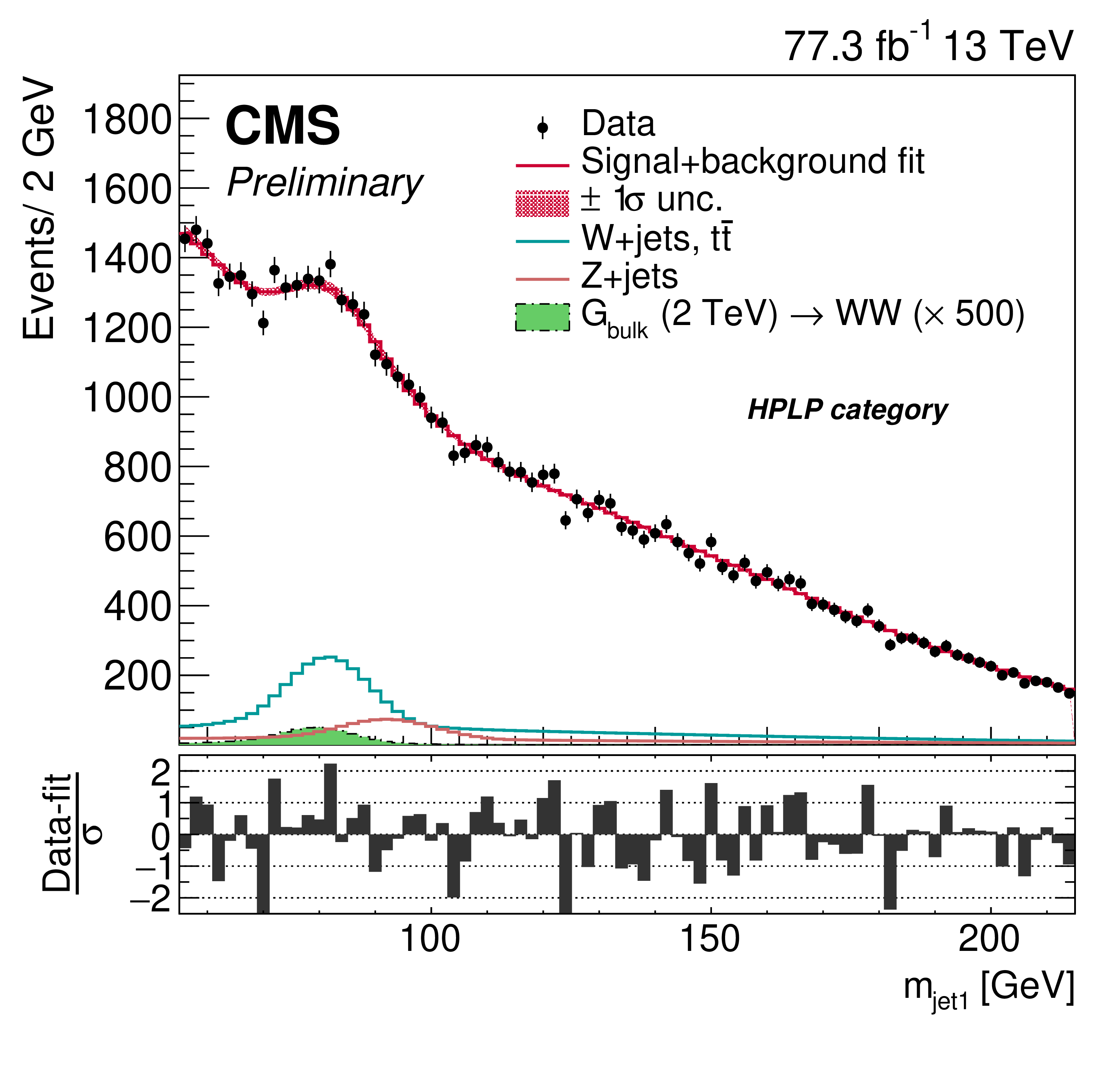
Figure 11:
Comparison between the fitted result and data distributions of ${m_\text {jet1}}$ (left), ${m_\text {jet2}}$ (middle), and ${m_\mathrm {VV}}$ (right) in the HPLP category. The background shape uncertainty is shown as a red shaded band, and the statistical uncertainties of the data are shown as vertical bars. An example of a signal distribution is overlaid, using an arbitrary normalisation. The corresponding pull distributions (Data-fit)/$\sigma $, where $\sigma = \sqrt {\sigma _\mathrm {data}^2 - \sigma _\mathrm {fit}^2}$ for a bin in ${m_\mathrm {VV}}$ to ensure a Gaussian pull-distribution as defined in [78], are shown below each ${m_\mathrm {VV}}$ plot. |
png pdf |
Figure 11-a:
Comparison between the fitted result and data distributions of ${m_\text {jet1}}$ in the HPLP category. The background shape uncertainty is shown as a red shaded band, and the statistical uncertainties of the data are shown as vertical bars. An example of a signal distribution is overlaid, using an arbitrary normalisation. The corresponding pull distributions (Data-fit)/$\sigma $, where $\sigma = \sqrt {\sigma _\mathrm {data}^2 - \sigma _\mathrm {fit}^2}$ for a bin in ${m_\mathrm {VV}}$ to ensure a Gaussian pull-distribution as defined in [78], are shown below the ${m_\mathrm {VV}}$ plot. |
png pdf |
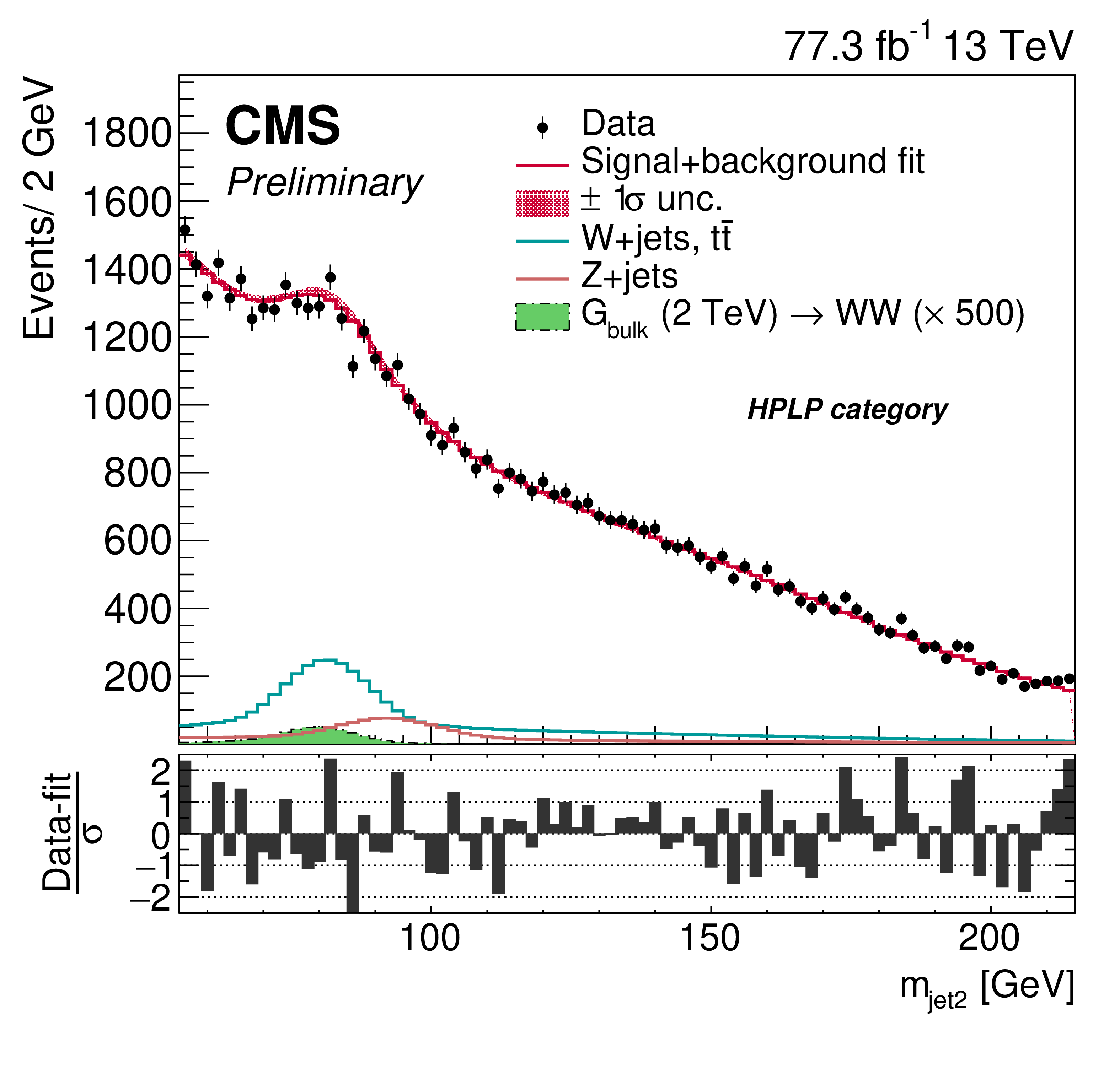
Figure 11-b:
Comparison between the fitted result and data distributions of ${m_\text {jet2}}$ in the HPLP category. The background shape uncertainty is shown as a red shaded band, and the statistical uncertainties of the data are shown as vertical bars. An example of a signal distribution is overlaid, using an arbitrary normalisation. The corresponding pull distributions (Data-fit)/$\sigma $, where $\sigma = \sqrt {\sigma _\mathrm {data}^2 - \sigma _\mathrm {fit}^2}$ for a bin in ${m_\mathrm {VV}}$ to ensure a Gaussian pull-distribution as defined in [78], are shown below the ${m_\mathrm {VV}}$ plot. |
png pdf |
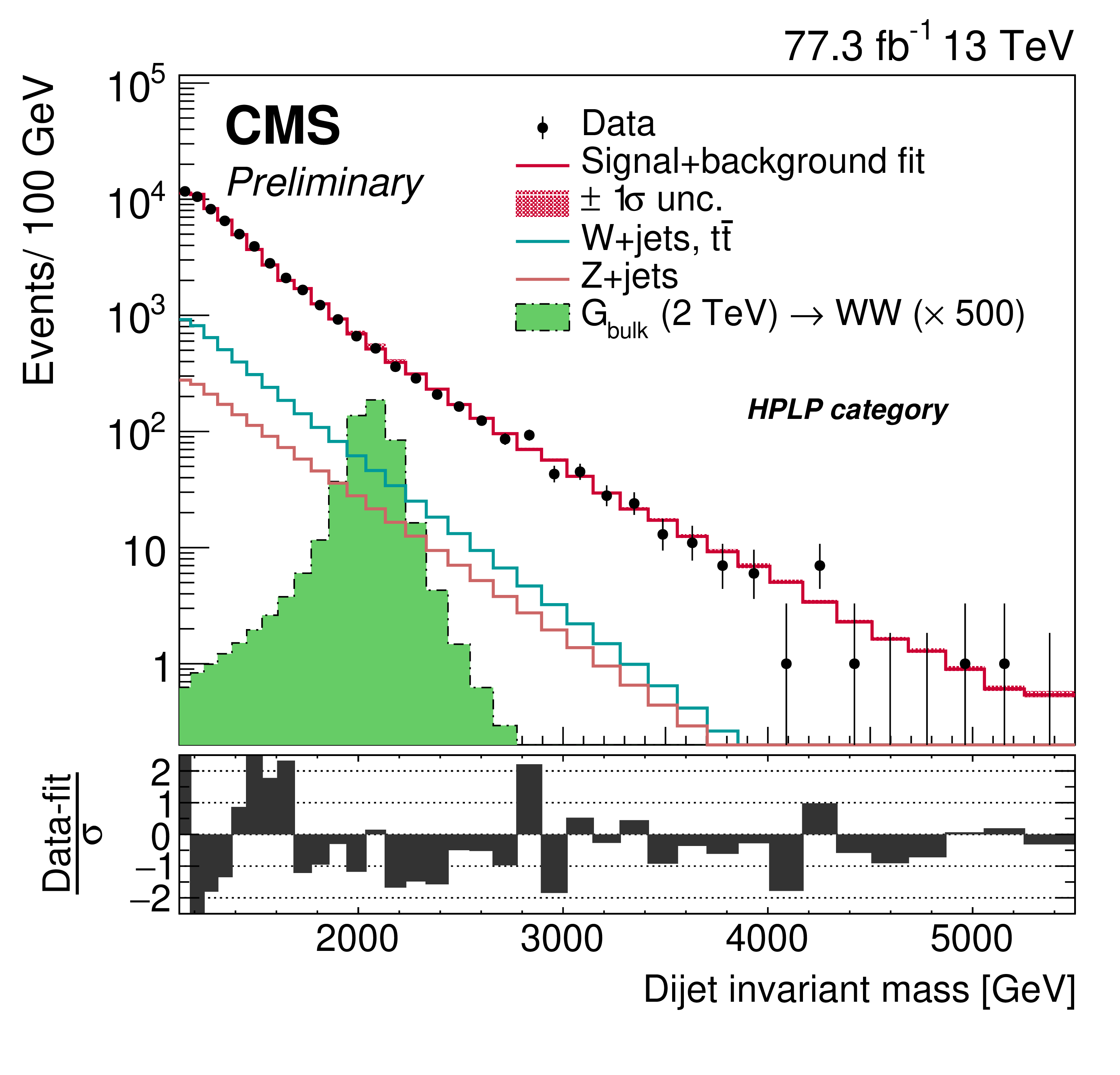
Figure 11-c:
Comparison between the fitted result and data distributions of ${m_\mathrm {VV}}$ in the HPLP category. The background shape uncertainty is shown as a red shaded band, and the statistical uncertainties of the data are shown as vertical bars. An example of a signal distribution is overlaid, using an arbitrary normalisation. The corresponding pull distributions (Data-fit)/$\sigma $, where $\sigma = \sqrt {\sigma _\mathrm {data}^2 - \sigma _\mathrm {fit}^2}$ for a bin in ${m_\mathrm {VV}}$ to ensure a Gaussian pull-distribution as defined in [78], are shown below the ${m_\mathrm {VV}}$ plot. |
png pdf |
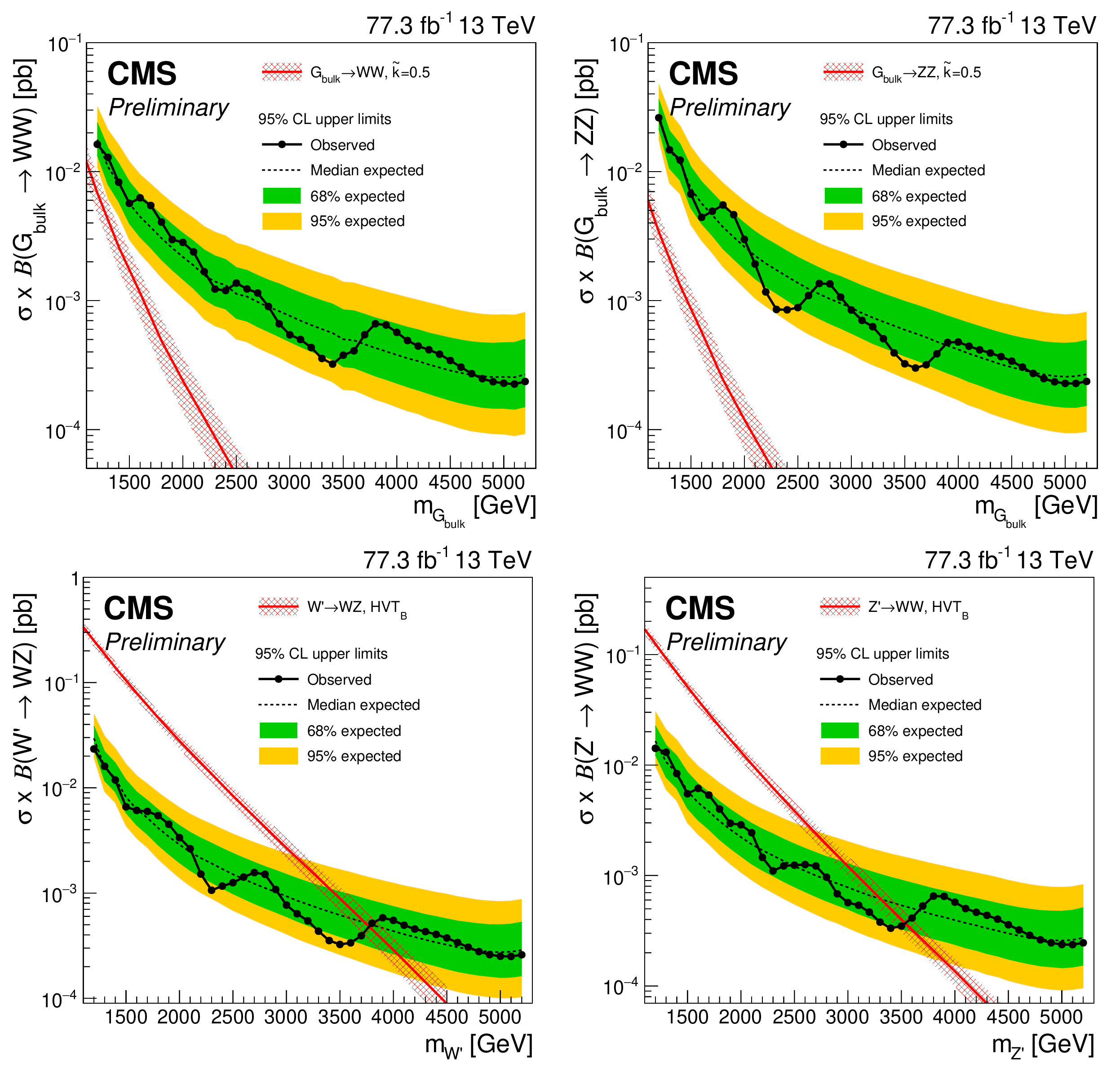
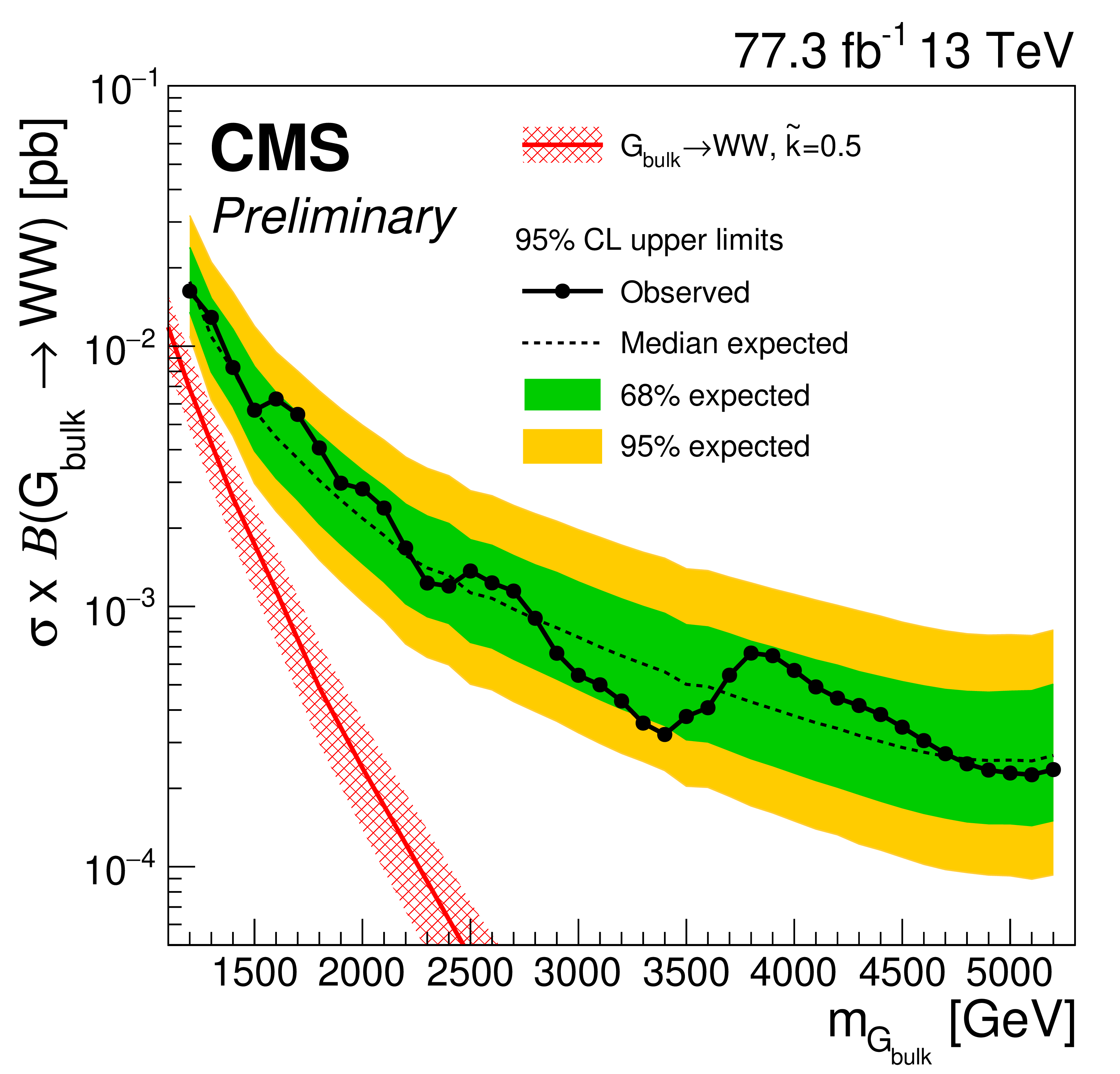
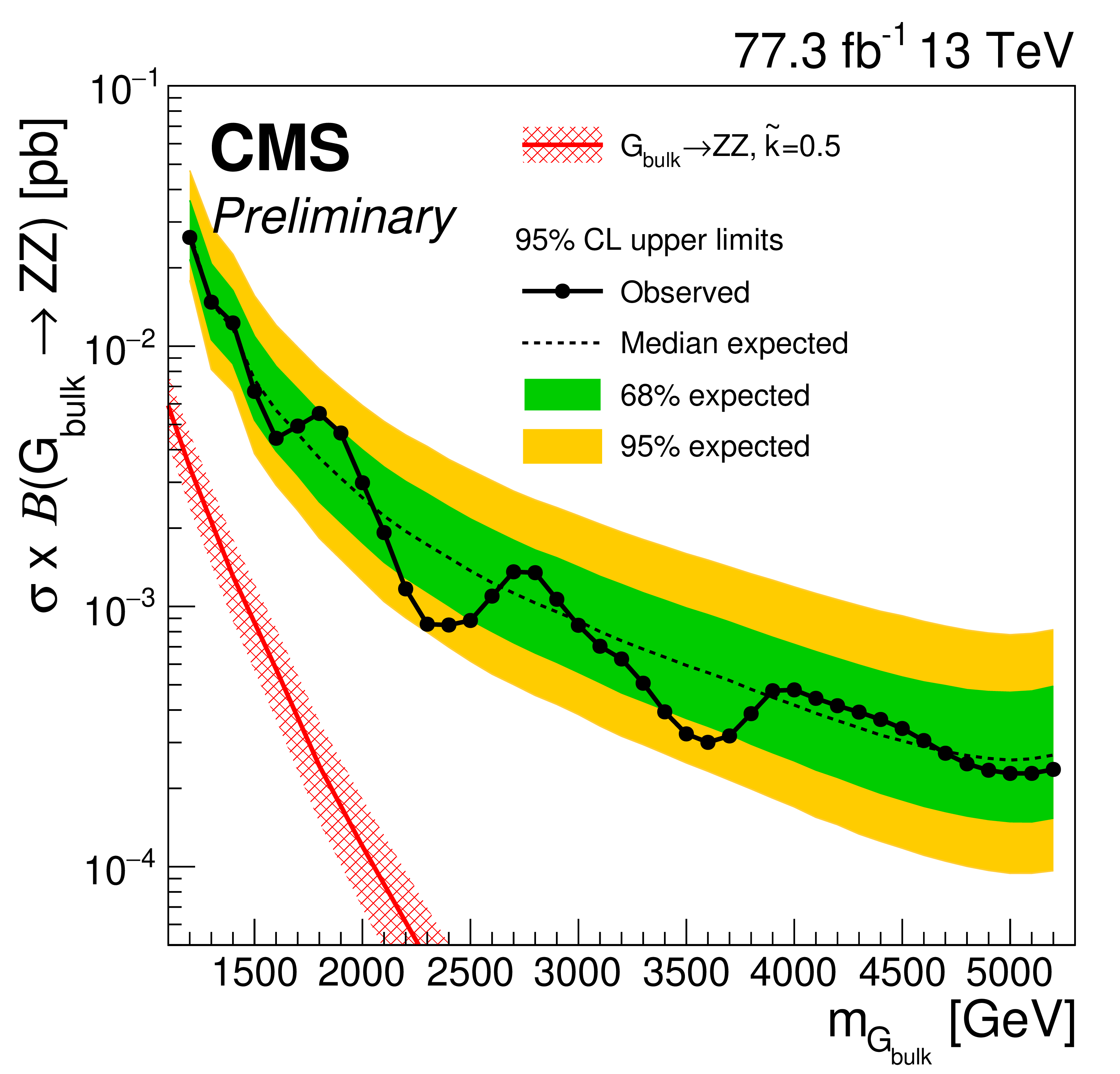
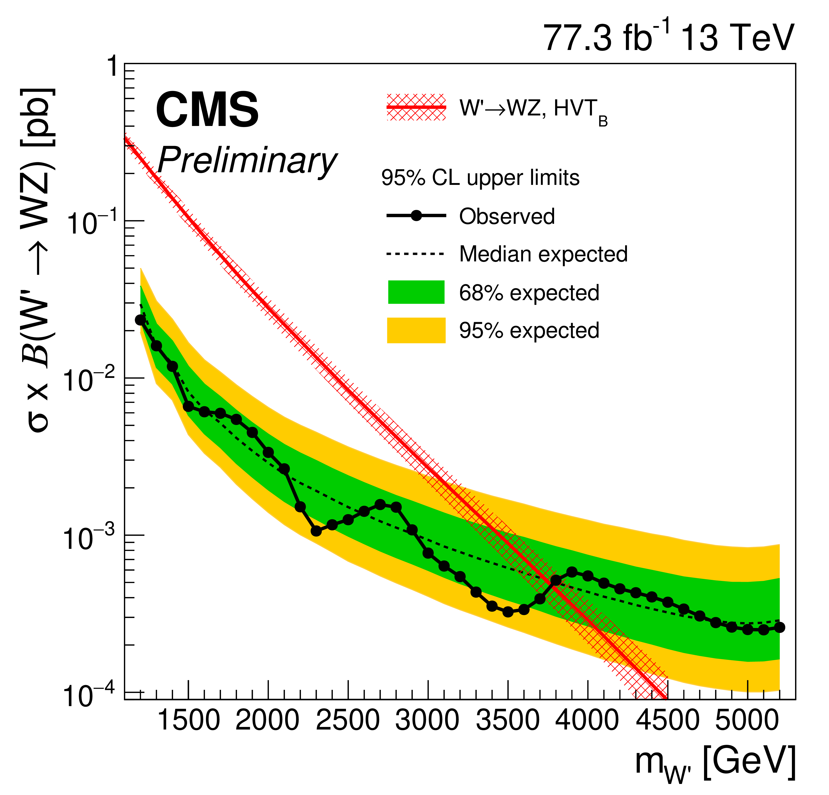
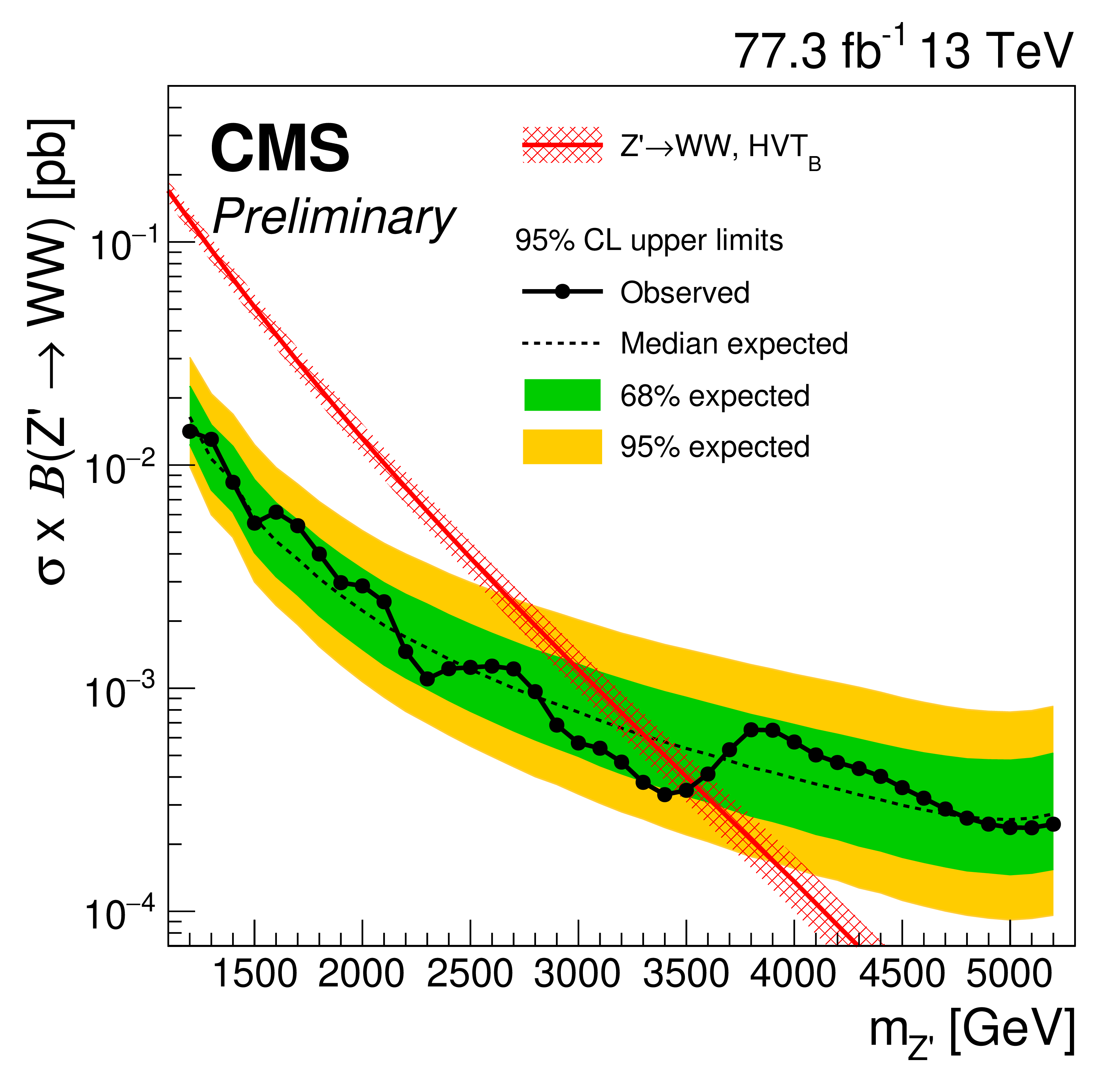
Figure 12:
Observed and expected limits obtained with 77.3 fb$^{-1}$ of 13 TeV data after combining categories of all purities for $ {{\mathrm {G}} _{\text {bulk}}} \rightarrow \mathrm{WW}$ (upper left), $ {{\mathrm {G}} _{\text {bulk}}} \rightarrow {\mathrm {Z}} {\mathrm {Z}} $ (upper right), $ {\mathrm {W}'} \rightarrow \mathrm{WZ} $ (lower left), and $ {\mathrm {Z}'} \rightarrow \mathrm{WW}$ (lower right) signals. |
png pdf |
Figure 12-a:
Observed and expected limits obtained with 77.3 fb$^{-1}$ of 13 TeV data after combining categories of all purities for $ {{\mathrm {G}} _{\text {bulk}}} \rightarrow \mathrm{WW}$ signal. |
png pdf |
Figure 12-b:
Observed and expected limits obtained with 77.3 fb$^{-1}$ of 13 TeV data after combining categories of all purities for $ {{\mathrm {G}} _{\text {bulk}}} \rightarrow {\mathrm {Z}} {\mathrm {Z}} $ signal. |
png pdf |
Figure 12-c:
Observed and expected limits obtained with 77.3 fb$^{-1}$ of 13 TeV data after combining categories of all purities for $ {\mathrm {W}'} \rightarrow \mathrm{WZ} $ signal. |
png pdf |
Figure 12-d:
Observed and expected limits obtained with 77.3 fb$^{-1}$ of 13 TeV data after combining categories of all purities for $ {\mathrm {Z}'} \rightarrow \mathrm{WW}$ signal. |
png pdf |
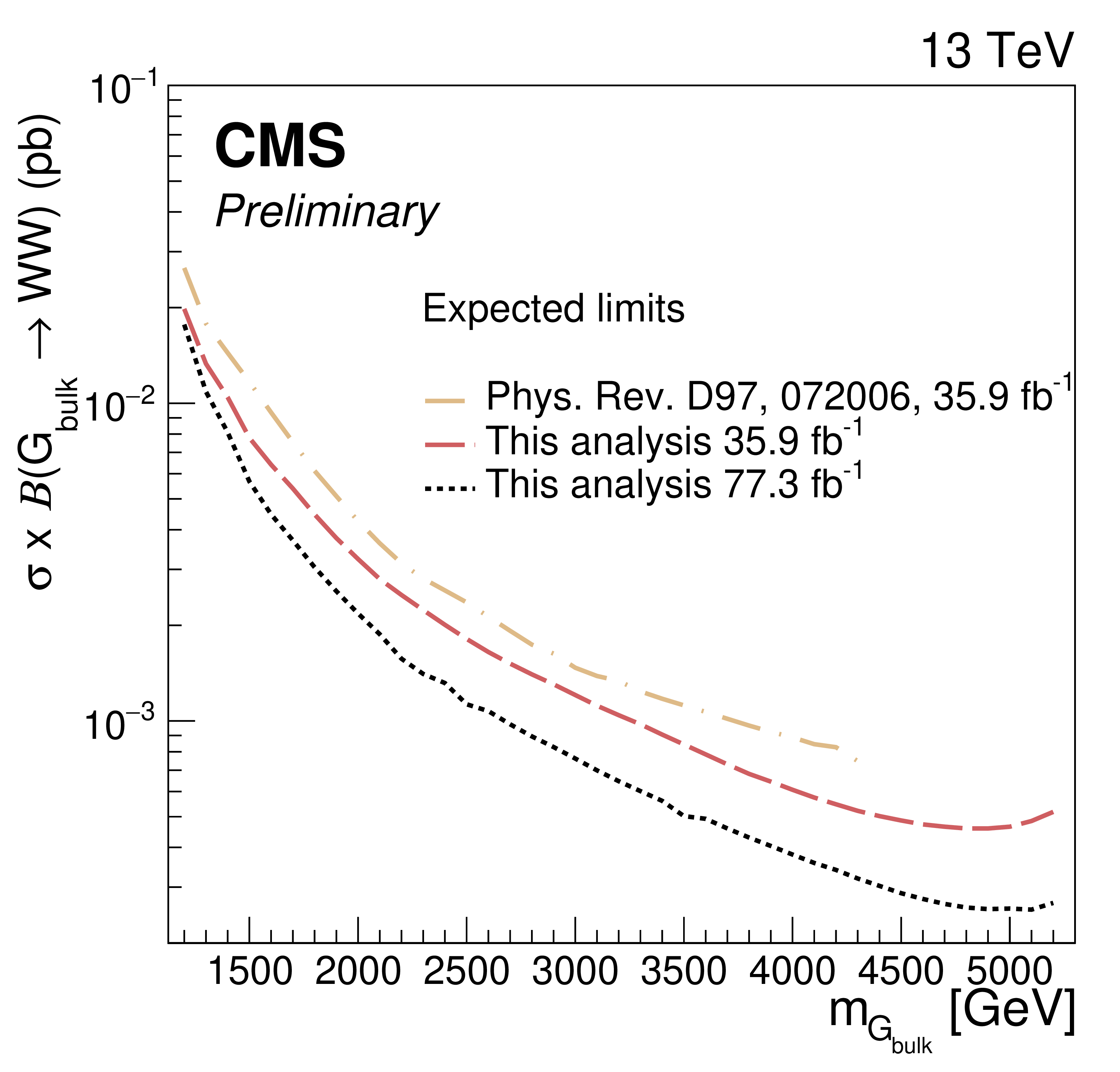
Figure 13:
Expected limits for a Bulk $G\rightarrow \mathrm{WW}$ signal using 35.9 fb$^{-1}$ of data collected in 2016 obtained using the multi-dimensional fit method presented here (pink line), compared to the result obtained using previous methods (beige line) [26]. The final limit obtained when combining data collected in 2016 and 2017 is also shown (black dotted line). |
| Tables | |
png pdf |
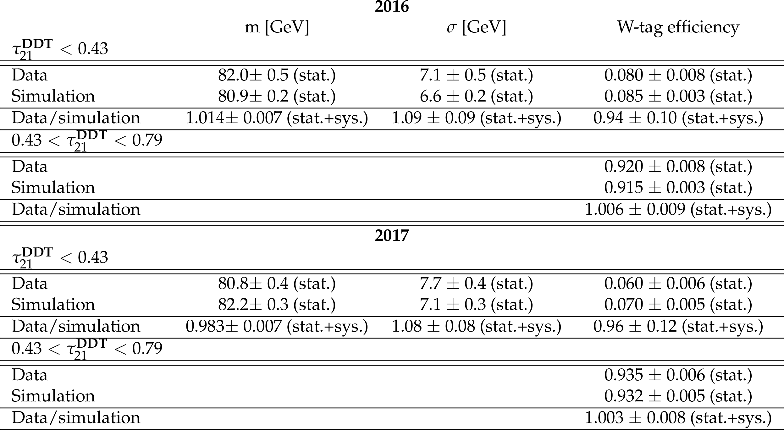
Table 1:
W-tagging efficiencies, and jet-mass scale and resolution scale factors as evaluated in the 2016 and 2017 data sets. |
png pdf |
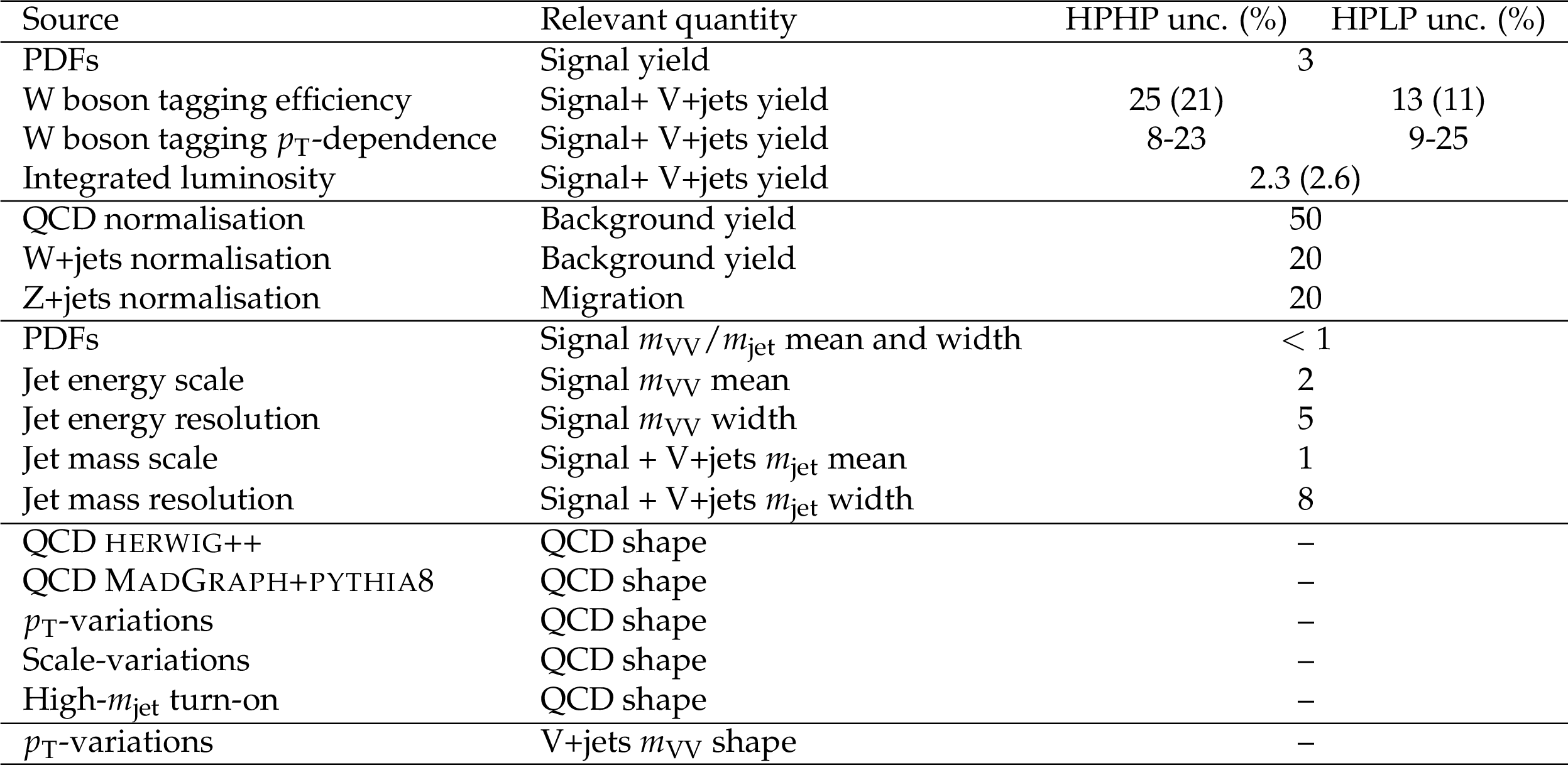
Table 2:
Summary of the systematic uncertainties and the quantities they affect. Numbers in parentheses correspond to uncertainties for the 2016 analysis if these differ from those for 2017. Dashes indicate shape variations that cannot be described by a single parameter, and are described in the text. |
png pdf |
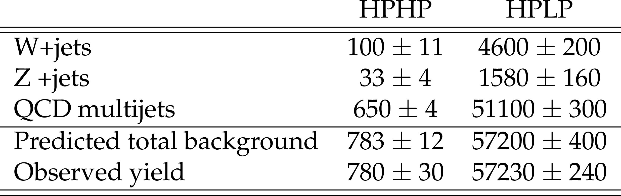
Table 3:
Observed and predicted background yields together with post-fit uncertainties in the two purity categories. |
| Summary |
| A search is presented for resonances with masses above 1.2 TeV that decay to WW, ZZ, or WZ. Each boson decays hadronically into one large-radius jet, resulting in dijet final states. This method yields improvements in sensitivity of up to 30% with respect to previous search methods used in CMS [26]. The new technique allows for placing additional constraints on systematic uncertainties concerning the signal through a measurement of the standard model W/Z+jets background. Hadronic W and Z boson decays are identified by requiring a jet with mass compatible with the W or Z boson mass, respectively. Additional information from jet substructure is used to reduce the background from multijet production. No evidence is found for a signal, and upper limits on the resonance production cross section are set as functions of the resonance mass. The results are interpreted within bulk graviton models and as W' and Z' resonances within the heavy vector triplet framework. For the heavy vector triplet model B, we exclude at 95% confidence level W' and Z' spin-1 resonances with masses below 3.8 and 3.5 TeV, respectively. In the narrow-width bulk graviton model, upper limits on the production cross sections for ${\mathrm{G}_{\text{bulk}}} \rightarrow \mathrm{W}\mathrm{W}$ are set in the range from 20 fb for a resonance mass of 1.2 TeV, to the most stringent limit of 0.2 fb for high resonance masses of 5.2 TeV TeV. In the case of ${\mathrm{G}_{\text{bulk}}} \rightarrow \mathrm{Z}\mathrm{Z}$, upper limits in the cross section are between 27 and 0.2 fb for bulk graviton masses between 1.2 and 5.2 TeV, respectively. In the narrow-width bulk graviton model, upper limits on the production cross sections are set in the range from 20 fb for a resonance mass of 1.2 TeV, to the most stringent limit of 0.2 fb for a resonance mass of 5.2 TeV TeV for ${\mathrm{G}_{\text{bulk}}} \rightarrow \mathrm{W}\mathrm{W}$. |
| References | ||||
| 1 | K. Agashe, H. Davoudiasl, G. Perez, and A. Soni | Warped Gravitons at the LHC and Beyond | PRD. 76 (2007) 036006 | hep-ph/0701186 |
| 2 | A. L. Fitzpatrick, J. Kaplan, L. Randall, and L.-T. Wang | Searching for the Kaluza-Klein Graviton in Bulk RS Models | JHEP 0709 (2007) 013 | hep-ph/0701150 |
| 3 | O. Antipin, D. Atwood, and A. Soni | Search for RS gravitons via W(L)W(L) decays | PLB. 666 (2008) 155--161 | 0711.3175 |
| 4 | L. Randall and R. Sundrum | A large mass hierarchy from a small extra dimension | PRL 83 (1999) 3370 | hep-ph/9905221 |
| 5 | L. Randall and R. Sundrum | An alternative to compactification | PRL 83 (1999) 4690--4693 | hep-th/9906064 |
| 6 | D. Pappadopulo, A. Thamm, R. Torre, and A. Wulzer | Heavy Vector Triplets: Bridging Theory and Data | JHEP 09 (2014) 060 | 1402.4431 |
| 7 | CMS Collaboration | Search for massive resonances in dijet systems containing jets tagged as W or Z boson decays in pp collisions at $ \sqrt{s} = $ 8 TeV | JHEP 08 (2014) 173 | CMS-EXO-12-024 1405.1994 |
| 8 | CMS Collaboration | Search for massive resonances decaying into pairs of boosted bosons in semi-leptonic final states at $ \sqrt{s}= $ 8 TeV | JHEP 1408 (2014) 174 | CMS-EXO-13-009 1405.3447 |
| 9 | ATLAS Collaboration | Search for $ W\!Z $ resonances in the fully leptonic channel using pp collisions at $ \sqrt{s} = $ 8 TeV collisions at ATLAS detector | PLB 737 (2014) 223 | 1406.4456 |
| 10 | CMS Collaboration | Search for new resonances decaying via WZ to leptons in proton-proton collisions at $ \sqrt{s} = $ 13 TeV | PLB 740 (2015) 83 | CMS-EXO-12-025 1407.3476 |
| 11 | CMS Collaboration | Search for narrow high-mass resonances in proton-proton collisions at $ \sqrt{s} = $ 8 TeV decaying to a Z and a Higgs boson | PLB 748 (2015) 255 | CMS-EXO-13-007 1502.04994 |
| 12 | CMS Collaboration | Search for heavy resonances that decay into a vector boson and a Higgs boson in hadronic final states at $ \sqrt{s} = $ 13 TeV | EPJC. 77 (2017) 636 | CMS-B2G-17-002 1707.01303 |
| 13 | CMS Collaboration | Search for heavy resonances decaying into a vector boson and a Higgs boson in final states with charged leptons, neutrinos, and b quarks | PLB 768 (2017) 137 | CMS-B2G-16-003 1610.08066 |
| 14 | ATLAS Collaboration | Search for resonant diboson production in the $ \mathrm {\ell \ell}q\bar{q} $ final state in $ pp $ collisions at $ \sqrt{s} = $ 8 TeV with the ATLAS detector | EPJC 75 (2015) 69 | 1409.6190 |
| 15 | ATLAS Collaboration | Search for production of $ WW/W\!Z $ resonances decaying to a lepton, neutrino and jets in $ pp $ collisions at $ \sqrt{s} = $ 8 TeV with the ATLAS detector | EPJC 75 (2015) 209 | 1503.04677 |
| 16 | ATLAS Collaboration | Search for a new resonance decaying to a $ W $ or $ Z $ boson and a Higgs boson in the $ \ell \ell / \ell \nu / \nu \nu + b \bar{b} $ final states with the ATLAS detector | EPJC 75 (2015) 263 | 1503.08089 |
| 17 | ATLAS Collaboration | Search for high-mass diboson resonances with boson-tagged jets in proton-proton collisions at $ \sqrt{s} = $ 8 TeV with the ATLAS detector | JHEP 12 (2015) 055 | 1506.00962 |
| 18 | CMS Collaboration | Search for a massive resonance decaying into a Higgs boson and a W or Z boson in hadronic final states in proton-proton collisions at $ \sqrt{s} = $ 8 TeV | JHEP 02 (2016) 145 | CMS-EXO-14-009 1506.01443 |
| 19 | CMS Collaboration | Search for massive WH resonances decaying into the $ \ell \nu \mathrm{b} \overline{\mathrm{b}} $ final state at $ \sqrt{s} = $ 8 TeV | EPJC 76 (2016) 237 | CMS-EXO-14-010 1601.06431 |
| 20 | CMS Collaboration | Search for heavy resonances decaying to two Higgs bosons in final states containing four b quarks | EPJC 76 (2016) 371 | CMS-EXO-12-053 1602.08762 |
| 21 | ATLAS Collaboration | Searches for heavy diboson resonances in $ pp $ collisions at $ \sqrt{s} = $ 13 TeV with the ATLAS detector | JHEP 09 (2016) 173 | 1606.04833 |
| 22 | CMS Collaboration | Search for massive resonances decaying into WW, WZ or ZZ bosons in proton-proton collisions at $ \sqrt{s} = $ 13 TeV | JHEP 03 (2017) 162 | CMS-B2G-16-004 1612.09159 |
| 23 | ATLAS Collaboration | Search for new resonances decaying to a $ W $ or $ Z $ boson and a Higgs boson in the $ \ell^+ \ell^- b\bar b $, $ \ell \nu b\bar b $, and $ \nu\bar{\nu} b\bar b $ channels with $ pp $ collisions at $ \sqrt{s} = $ 13 TeV with the ATLAS detector | PLB 765 (2017) 32 | 1607.05621 |
| 24 | ATLAS Collaboration | Search for heavy resonances decaying to a $ W $ or $ Z $ boson and a Higgs boson in the $ q\bar{q}^{(\prime)}b\bar{b} $ final state in $ pp $ collisions at $ \sqrt{s} = $ 13 TeV with the ATLAS detector | PLB 774 (2017) 494 | 1707.06958 |
| 25 | ATLAS Collaboration | Search for diboson resonances with boson-tagged jets in $ pp $ collisions at $ \sqrt{s}= $ 13 TeV with the ATLAS detector | PLB. 777 (2018) 91--113 | 1708.04445 |
| 26 | CMS Collaboration | Search for massive resonances decaying into $ WW $, $ WZ $, $ ZZ $, $ qW $, and $ qZ $ with dijet final states at $ \sqrt{s}=13\text{}\text{}\mathrm{TeV} $ | PRD. 97 (2018) 072006 | CMS-B2G-17-001 1708.05379 |
| 27 | CMS Collaboration | Search for a heavy resonance decaying to a pair of vector bosons in the lepton plus merged jet final state at $ \sqrt{s}= $ 13 TeV | JHEP 05 (2018) 088 | CMS-B2G-16-029 1802.09407 |
| 28 | ATLAS Collaboration | Search for diboson resonances in hadronic final states in 139$ fb$^{-1} of pp collisions at $ \sqrt{s} = $ 13 TeV with the ATLAS detector | ATLAS Conference Note ATLAS-CONF-2019-003 | |
| 29 | CMS Collaboration | The CMS experiment at the CERN LHC | JINST 3 (2008) S08004 | CMS-00-001 |
| 30 | CMS Collaboration | Description and performance of track and primary-vertex reconstruction with the CMS tracker | JINST 9 (2014) P10009 | CMS-TRK-11-001 1405.6569 |
| 31 | M. Cacciari, G. P. Salam, and G. Soyez | The anti-$ k_t $ jet clustering algorithm | JHEP 04 (2008) 063 | 0802.1189 |
| 32 | M. Cacciari, G. P. Salam, and G. Soyez | FastJet user manual | EPJC 72 (2012) 1896 | 1111.6097 |
| 33 | C. Grojean, E. Salvioni, and R. Torre | A weakly constrained W' at the early LHC | JHEP 07 (2011) 002 | 1103.2761 |
| 34 | E. Salvioni, G. Villadoro, and F. Zwirner | Minimal Z' models: present bounds and early LHC reach | JHEP 11 (2009) 068 | 0909.1320 |
| 35 | B. Bellazzini, C. Cs\'aki, and J. Serra | Composite Higgses | EPJC. 74 (2014) 2766 | 1401.2457 |
| 36 | R. Contino, D. Pappadopulo, D. Marzocca, and R. Rattazzi | On the effect of resonances in composite higgs phenomenology | JHEP 2011 (2011) | |
| 37 | D. Marzocca, M. Serone, and J. Shu | General composite Higgs models | JHEP 08 (2012) 013 | 1205.0770 |
| 38 | D. Greco and D. Liu | Hunting composite vector resonances at the LHC: naturalness facing data | JHEP 1412 (2014) 126 | 1410.2883 |
| 39 | K. Lane and L. Pritchett | The light composite Higgs boson in strong extended technicolor | JHEP 06 (2017) 140 | 1604.07085 |
| 40 | M. Schmaltz and D. Tucker-Smith | Little Higgs review | Ann. Rev. Nucl. Part. Sci. 55 (2005) 229--270 | hep-ph/0502182 |
| 41 | N. Arkani-Hamed, A. Cohen, E. Katz, and A. Nelson | The Littlest Higgs | JHEP 0207 (2002) 034 | hep-ph/0206021 |
| 42 | J. Alwall et al. | The automated computation of tree-level and next-to-leading order differential cross sections, and their matching to parton shower simulations | JHEP 07 (2014) 079 | 1405.0301 |
| 43 | T. Sjostrand et al. | An Introduction to PYTHIA 8.2 | CPC 191 (2015) 159--177 | 1410.3012 |
| 44 | NNPDF Collaboration | Parton distributions for the LHC Run II | JHEP 04 (2015) 040 | 1410.8849 |
| 45 | CMS Collaboration | Event generator tunes obtained from underlying event and multiparton scattering measurements | EPJC. 76 (2016) 155 | CMS-GEN-14-001 1512.00815 |
| 46 | CMS Collaboration | Extraction and validation of a new set of CMS PYTHIA8 tunes from underlying-event measurements | CMS-PAS-GEN-17-001 | CMS-PAS-GEN-17-001 |
| 47 | J. Alwall et al. | Comparative study of various algorithms for the merging of parton showers and matrix elements in hadronic collisions | EPJC. 53 (2008) 473 | 0706.2569 |
| 48 | S. Alioli et al. | Jet pair production in POWHEG | JHEP 04 (2011) 081 | 1012.3380 |
| 49 | P. Nason | A New method for combining NLO QCD with shower Monte Carlo algorithms | JHEP 11 (2004) 040 | hep-ph/0409146 |
| 50 | S. Frixione, P. Nason, and C. Oleari | Matching NLO QCD computations with Parton Shower simulations: the POWHEG method | JHEP 11 (2007) 070 | 0709.2092 |
| 51 | S. Alioli, P. Nason, C. Oleari, and E. Re | A general framework for implementing NLO calculations in shower Monte Carlo programs: the POWHEG BOX | JHEP 06 (2010) 043 | 1002.2581 |
| 52 | M. Bahr et al. | Herwig++ physics and manual | EPJC 58 (2008) 639 | 0803.0883 |
| 53 | S. Alioli, S.-O. Moch, and P. Uwer | Hadronic top-quark pair-production with one jet and parton showering | JHEP 01 (2012) 137 | 1110.5251 |
| 54 | S. Kallweit et al. | NLO electroweak automation and precise predictions for W+multijet production at the LHC | JHEP 04 (2015) 012 | 1412.5157 |
| 55 | S. Kallweit et al. | NLO QCD+EW predictions for V+jets including off-shell vector-boson decays and multijet merging | JHEP 04 (2016) 021 | 1511.08692 |
| 56 | NNPDF Collaboration | Parton distributions from high-precision collider data | EPJC. 77 (2017) 663 | 1706.00428 |
| 57 | GEANT4 Collaboration | GEANT4 - a simulation toolkit | NIMA 506 (2003) 250 | |
| 58 | CMS Collaboration | Particle-flow reconstruction and global event description with the CMS detector | JINST 12 (2017) P10003 | CMS-PRF-14-001 1706.04965 |
| 59 | D. Bertolini, P. Harris, M. Low, and N. Tran | Pileup per particle identification | JHEP 2014 (2014) 1 | |
| 60 | CMS Collaboration | Jet algorithms performance in 13 TeV data | CMS-PAS-JME-16-003 | CMS-PAS-JME-16-003 |
| 61 | CMS Collaboration | Determination of Jet Energy Calibration and Transverse Momentum Resolution in CMS | JINST 6 (2011) P11002 | CMS-JME-10-011 1107.4277 |
| 62 | M. Cacciari, G. P. Salam, and G. Soyez | The Catchment Area of Jets | JHEP 04 (2008) 005 | 0802.1188 |
| 63 | M. Dasgupta, A. Fregoso, S. Marzani, and G. P. Salam | Towards an understanding of jet substructure | JHEP 1309 (2013) 029 | 1307.0007 |
| 64 | J. M. Butterworth, A. R. Davison, M. Rubin, and G. P. Salam | Jet substructure as a new Higgs search channel at the LHC | PRL 100 (2008) 242001 | 0802.2470 |
| 65 | A. J. Larkoski, S. Marzani, G. Soyez, and J. Thaler | Soft Drop | JHEP 1405 (2014) 146 | 1402.2657 |
| 66 | J. Thaler and K. Van Tilburg | Maximizing Boosted Top Identification by Minimizing N-subjettiness | JHEP 1202 (2012) 093 | 1108.2701 |
| 67 | S. Catani, \relax Yu. L. Dokshitzer, M. H. Seymour, and B. R. Webber | Longitudinally invariant $ K_t $ clustering algorithms for hadron hadron collisions | NPB 406 (1993) 187 | |
| 68 | M. Wobisch and T. Wengler | Hadronization corrections to jet cross-sections in deep inelastic scattering | in Monte Carlo generators for HERA physics 1998 | hep-ph/9907280 |
| 69 | J. Dolen et al. | Thinking outside the ROCs: Designing Decorrelated Taggers (DDT) for jet substructure | JHEP 05 (2016) 156 | 1603.00027 |
| 70 | D. Krohn, J. Thaler, and L.-T. Wang | Jet Trimming | JHEP 02 (2010) 084 | 0912.1342 |
| 71 | CMS Collaboration | Performance of CMS muon reconstruction in $ pp $ collision events at $ \sqrt{s}= $ 7 TeV | JINST 7 (2012) P10002 | CMS-MUO-10-004 1206.4071 |
| 72 | CMS Collaboration | Performance of electron reconstruction and selection with the CMS detector in proton-proton collisions at $ \sqrt{s} = 8{TeV} $ | JINST 10 (2015) P06005 | CMS-EGM-13-001 1502.02701 |
| 73 | CMS Collaboration | Measurement of differential cross sections for top quark pair production using the lepton+jets final state in proton-proton collisions at 13 TeV | PRD 95 (2017) 092001 | CMS-TOP-16-008 1610.04191 |
| 74 | K. S. Cranmer | Kernel estimation in high-energy physics | CPC 136 (2001) 198--207 | hep-ex/0011057 |
| 75 | A. L. Read | Presentation of search results: the $ \rm CL_s $ technique | JPG 28 (2002) 2693 | |
| 76 | T. Junk | Confidence level computation for combining searches with small statistics | NIMA 434 (1999) 435 | hep-ex/9902006 |
| 77 | G. Cowan, K. Cranmer, E. Gross, and O. Vitells | Asymptotic formulae for likelihood-based tests of new physics | EPJC 71 (2011) 1554 | 1007.1727 |
| 78 | L. Demortier and L. Lyons | Everything you always wanted to know about pulls | CDF/ANAL/PUBLIC/5776, CDF, February | |
|
|
Compact Muon Solenoid LHC, CERN |
|

|

|

|

|

|