

Compact Muon Solenoid
LHC, CERN
| CMS-BPH-24-002 ; CERN-EP-2025-118 | ||
| Determination of the spin and parity of all-charm tetraquarks | ||
| CMS Collaboration | ||
| 9 June 2025 | ||
| Nature 648 (2025) 58 | ||
| Abstract: The traditional quark model [1, 2] accounts for the existence of baryons, such as protons and neutrons, which consist of three quarks, as well as mesons, composed of a quark-antiquark pair. Only recently has substantial evidence started to accumulate for exotic states composed of four or five quarks and antiquarks [3]. The exact nature of their internal structure remains uncertain [4, 5, 6, 7, 8, 8, 9, 10, 11, 12, 13, 14, 15, 16, 17, 18, 19, 20, 21, 22, 23, 24, 25, 26, 27, 28, 29]. This paper reports the first measurement of quantum numbers of the recently discovered family of three all-charm tetraquarks [30, 31, 32], using data collected by the CMS experiment at the Large Hadron Collider from 2016 to 2018 [33, 34]. The angular analysis techniques developed for the discovery and characterization of the Higgs boson [35, 36, 37] have been applied to the new exotic states. Here we show that the quantum numbers for parity $ P $ and charge conjugation $ C $ symmetries are found to be $ + $1. The spin $ J $ of these exotic states is determined to be consistent with 2$ \hbar $, while 0$ \hbar $ and 1$ \hbar $ are excluded at 95% and 99% confidence level, respectively. The $ J^{PC}= $ 2$^{++} $ assignment implies particular configurations of constituent spins and orbital angular momenta, which constrain the possible internal structure of these tetraquarks. | ||
| Links: e-print arXiv:2506.07944 [hep-ex] (PDF) ; CDS record ; inSPIRE record ; HepData record ; Physics Briefing ; CADI line (restricted) ; | ||
| Figures | |
png pdf |
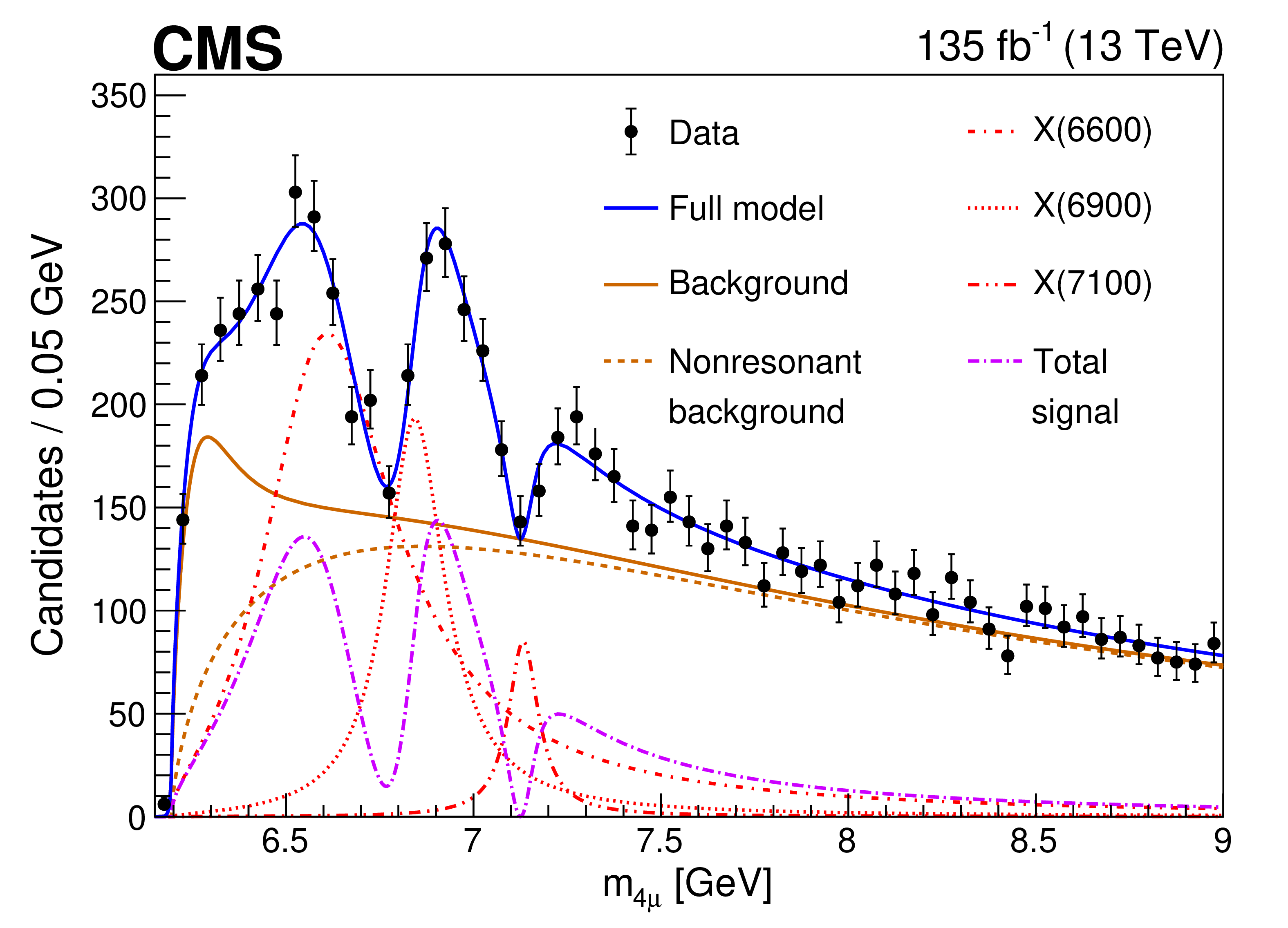
Figure 1:
Candidates for all-charm tetraquarks. The $ \mathrm{J}/\psi \mathrm{J}/\psi\to\mu^{+}\mu^{-}\mu^{+}\mu^{-} $ invariant mass $ m_{4\mu} $ spectrum shows the three exotic states, X(6600), X(6900), and X(7100). Parameterizations of these states are displayed both individually and as a combined signal that includes quantum-mechanical interference (denoted by ``Total signal"). The full model [32] incorporates both signal and background components, with the background originating from di-$ \mathrm{J}/\psi $ production, including contributions from nonresonant production and an enhancement near the kinematic threshold of 6.2 GeV. |
png pdf |
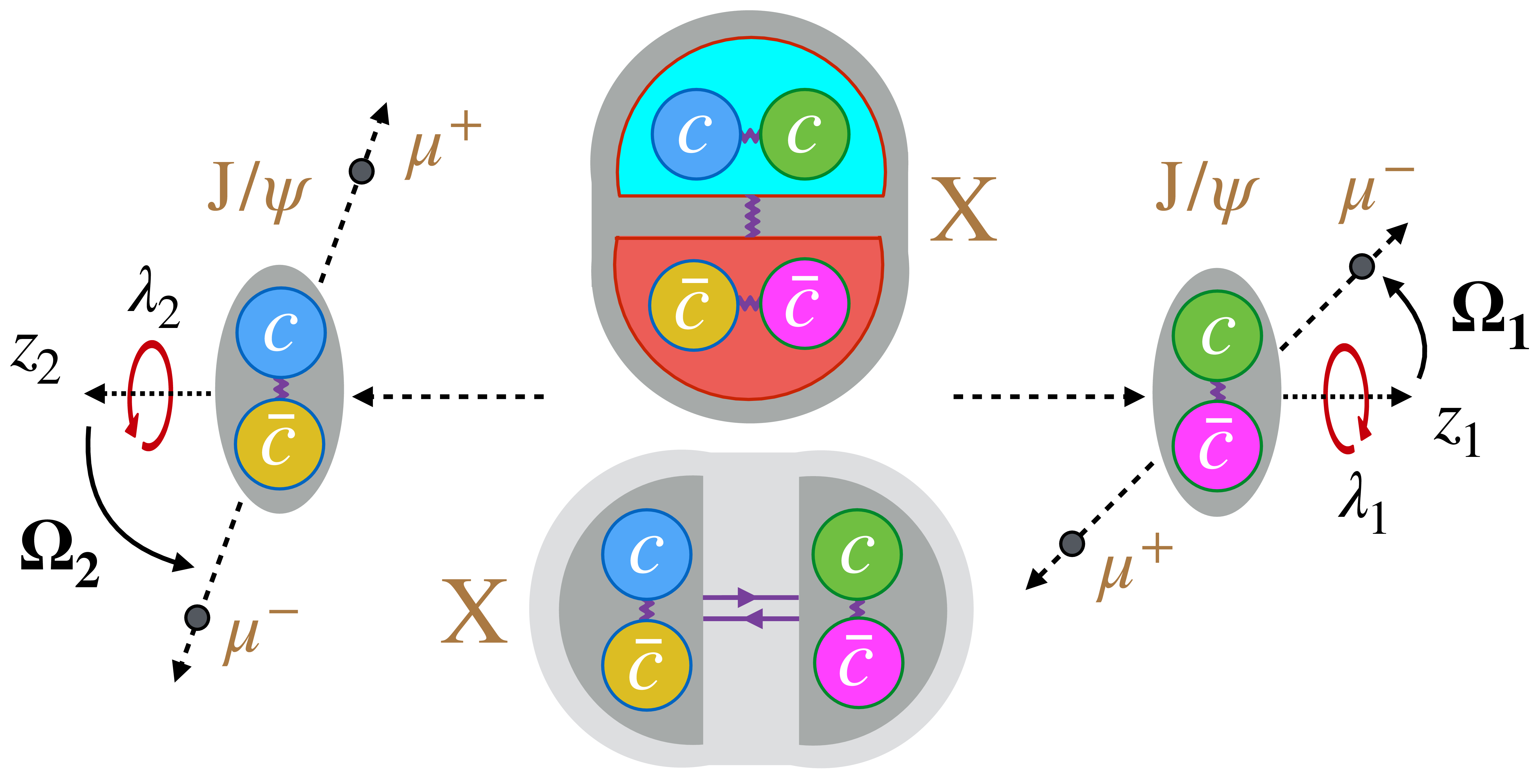
Figure 2:
{Internal structure models for the particle $ \mathrm{X} $.} The particle $ \mathrm{X} $, composed of $ {\mathrm{c}}{\mathrm{c}}{\overline{\mathrm{c}}}{\overline{\mathrm{c}}} $, is shown at rest. Two models of the internal structure of $ \mathrm{X} $ are presented: a tightly-bound tetraquark (upper) and a loosely-bound molecule of two mesons (lower). The colours assigned to individual quarks or quark pairs denote possible colour charge assignments in strong interactions, where attractive forces are mediated by gluon exchange (shown as wavy lines) and meson exchange (shown as a solid pair of arrows). The $ \mathrm{X} $ decays into two $ \mathrm{J}/\psi $ mesons with spin projections $ \lambda_i $ along their respective directions of motion; each meson then decays into a $ \mu^{+}\mu^{-} $ pair. The polar and azimuthal angles $ \mathbf{\Omega}_{i}=(\theta_{i}, \Phi_{i}) $ describe the direction of the $ \mu^{-} $ relative to the $ z_i $ axis, which is defined to point opposite to the $ \mathrm{X} $ direction in the centre-of-mass frame of the corresponding $ \mathrm{J}/\psi $ meson, for $ i = $ 1 and 2. |
png pdf |
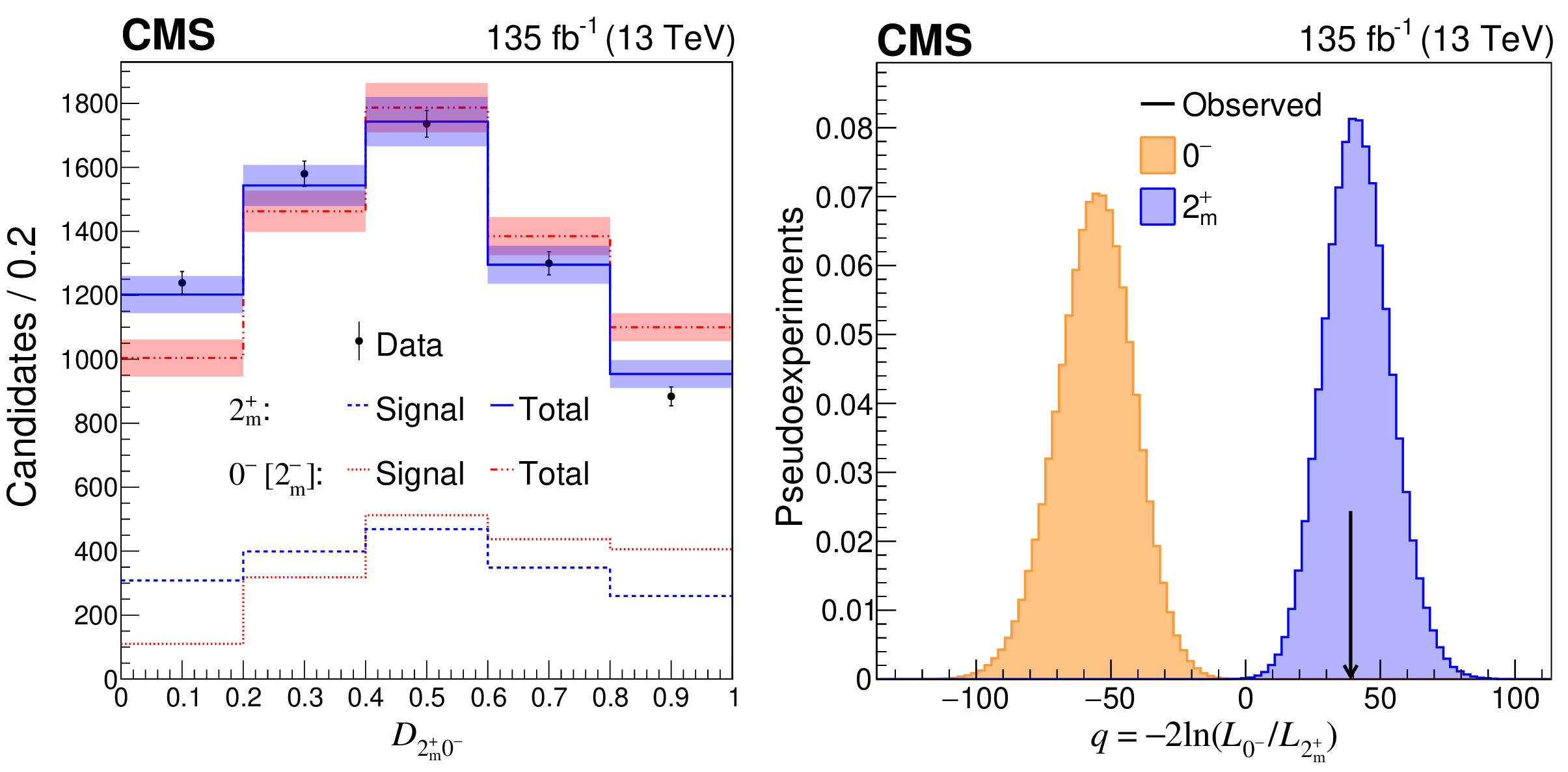
Figure 3:
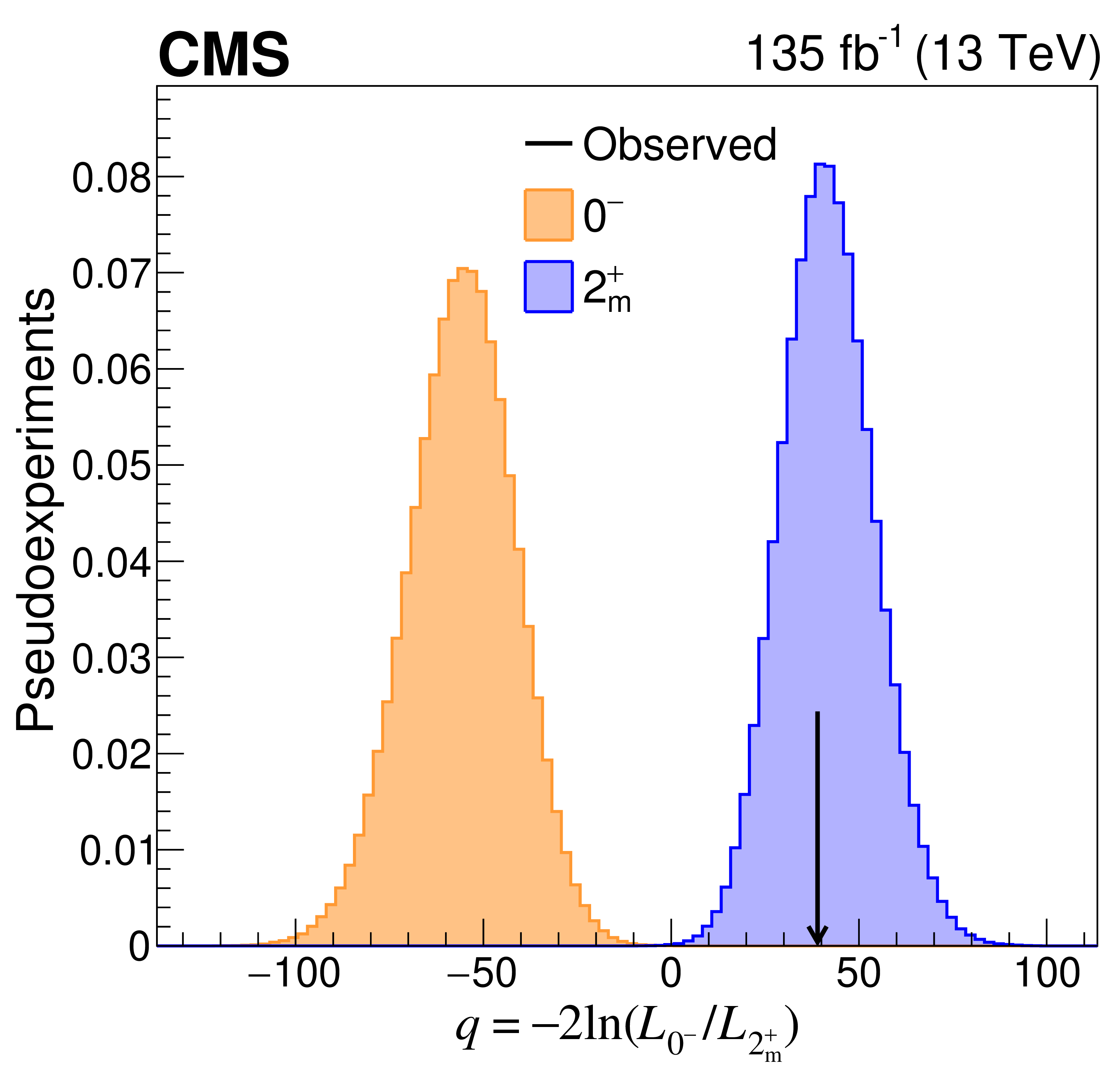
Analysis of angular distributions. Left: Distributions of $ \mathcal{D}_{2_m^{+}0^{-}} $ for the $ 0^{-} $, 2 $ _m^{-} $, and 2 $ _m^{+} $ models in the range 6.2 $ < m_{4\mu} < $ 8.0 GeV. Distributions for signal only (dashed) and for signal plus background (solid and dash-dot-dotted) models are compared to the experimental data points with error bars, with uncertainty bands representing post-fit model uncertainties, which are partially correlated with the data. The $ 0^{-} $ and 2 $ _m^{-} $ distributions are identical apart from systematic uncertainties arising from polarization effects. Right: Normalized distributions of the test statistic $ q=-2{\ln(\mathcal{L}_{ 0 ^{-}}/\mathcal{L}_{2^{+} _m})} $ from pseudoexperiments generated under the 2 $ _m^{+} $ (blue/right) and $ 0^{-} $ (orange/left) hypotheses, with the arrow indicating the observed value $ q_\text{obs} $. |
png pdf |
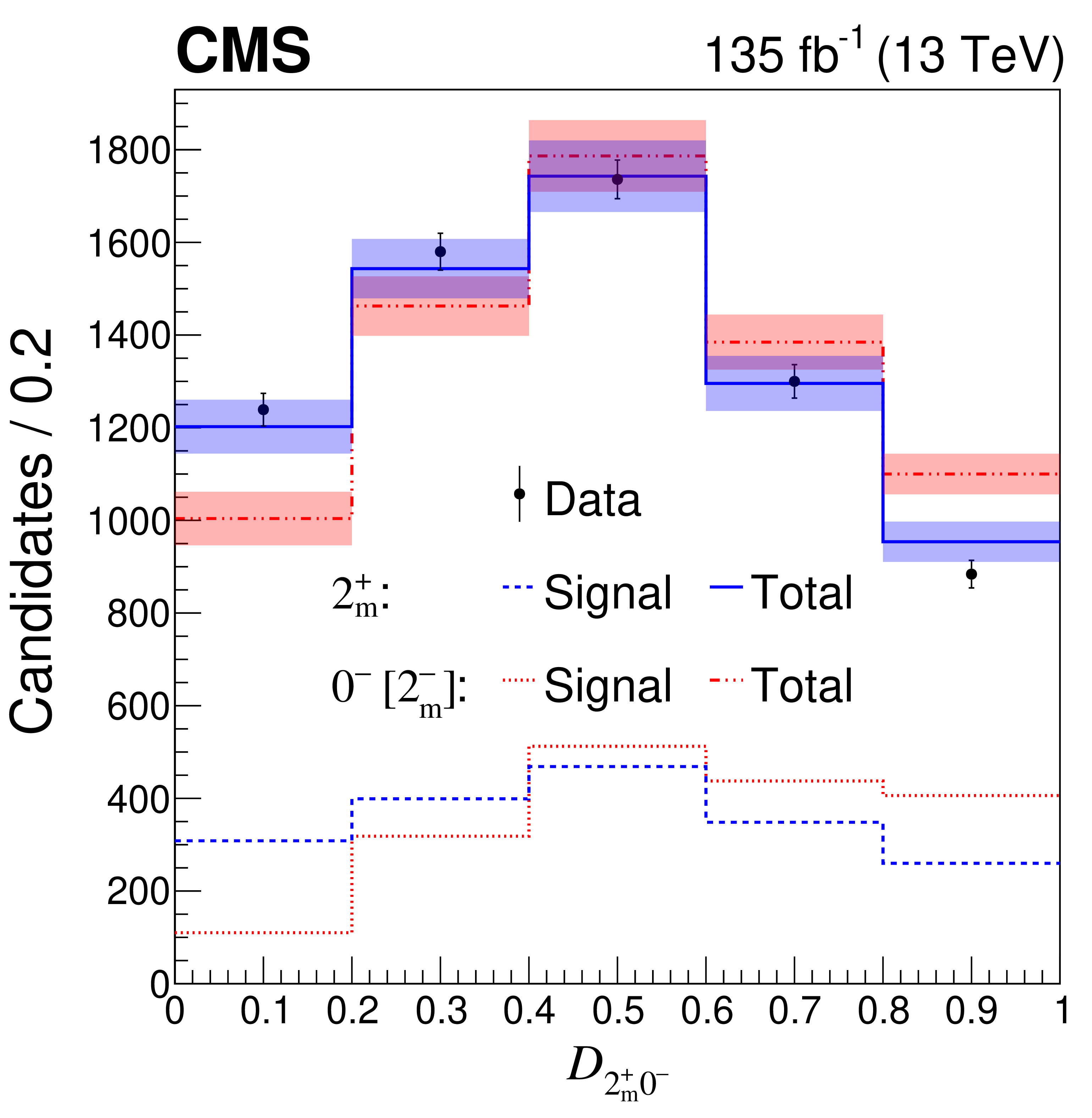
Figure 3-a:
Analysis of angular distributions. Left: Distributions of $ \mathcal{D}_{2_m^{+}0^{-}} $ for the $ 0^{-} $, 2 $ _m^{-} $, and 2 $ _m^{+} $ models in the range 6.2 $ < m_{4\mu} < $ 8.0 GeV. Distributions for signal only (dashed) and for signal plus background (solid and dash-dot-dotted) models are compared to the experimental data points with error bars, with uncertainty bands representing post-fit model uncertainties, which are partially correlated with the data. The $ 0^{-} $ and 2 $ _m^{-} $ distributions are identical apart from systematic uncertainties arising from polarization effects. Right: Normalized distributions of the test statistic $ q=-2{\ln(\mathcal{L}_{ 0 ^{-}}/\mathcal{L}_{2^{+} _m})} $ from pseudoexperiments generated under the 2 $ _m^{+} $ (blue/right) and $ 0^{-} $ (orange/left) hypotheses, with the arrow indicating the observed value $ q_\text{obs} $. |
png pdf |
Figure 3-b:
Analysis of angular distributions. Left: Distributions of $ \mathcal{D}_{2_m^{+}0^{-}} $ for the $ 0^{-} $, 2 $ _m^{-} $, and 2 $ _m^{+} $ models in the range 6.2 $ < m_{4\mu} < $ 8.0 GeV. Distributions for signal only (dashed) and for signal plus background (solid and dash-dot-dotted) models are compared to the experimental data points with error bars, with uncertainty bands representing post-fit model uncertainties, which are partially correlated with the data. The $ 0^{-} $ and 2 $ _m^{-} $ distributions are identical apart from systematic uncertainties arising from polarization effects. Right: Normalized distributions of the test statistic $ q=-2{\ln(\mathcal{L}_{ 0 ^{-}}/\mathcal{L}_{2^{+} _m})} $ from pseudoexperiments generated under the 2 $ _m^{+} $ (blue/right) and $ 0^{-} $ (orange/left) hypotheses, with the arrow indicating the observed value $ q_\text{obs} $. |
png pdf |
Figure 4:
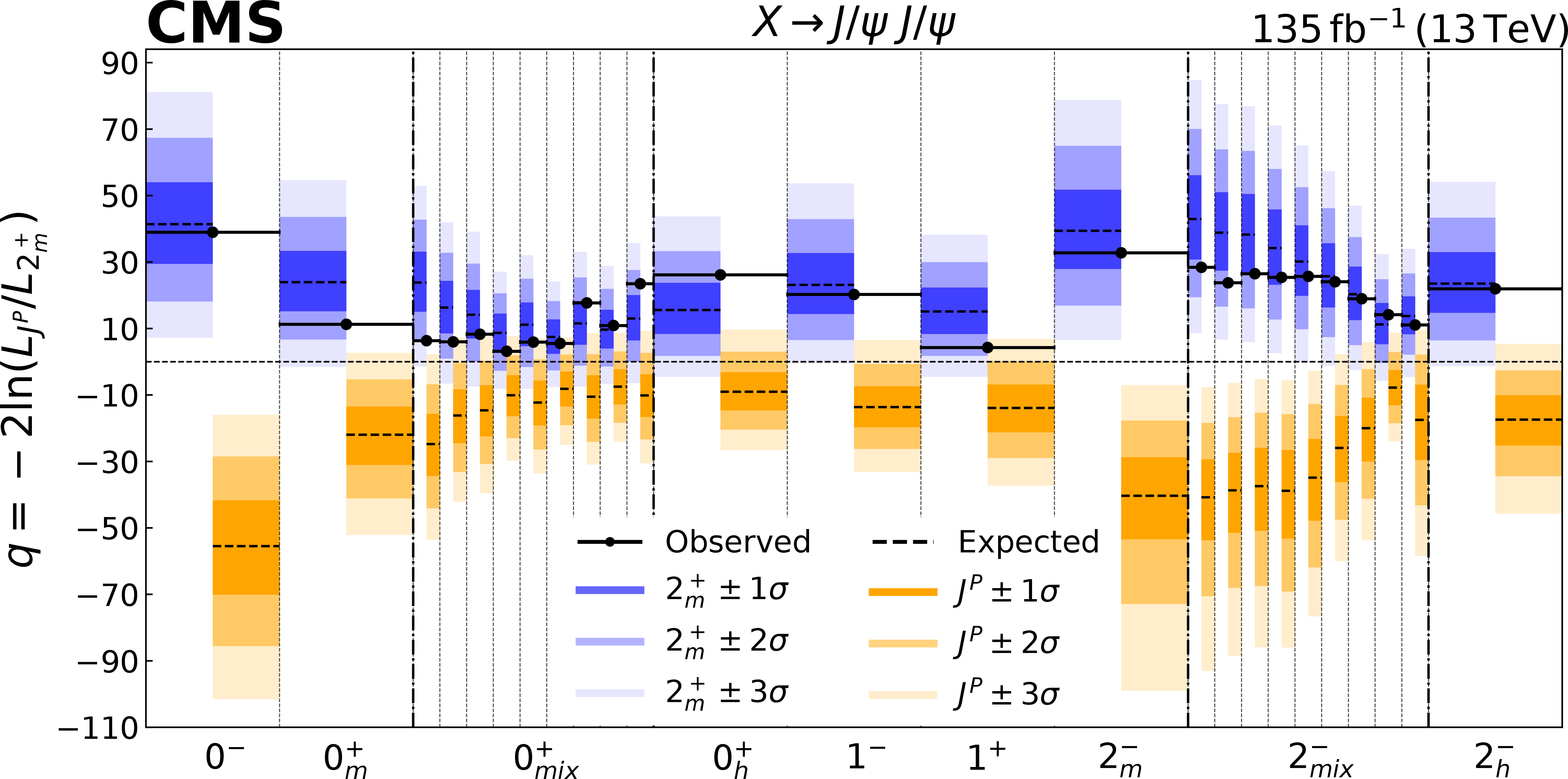
Summary of statistical tests. Distributions of the test statistic $ q $ for various $ J_i^{P} $ hypotheses tested against the 2 $ _m^{+} $ model. The observed $ q_\text{obs} $ values are indicated by the black dots. The expected median and the 68.3%, 95.4%, and 99.7% confidence level regions for the 2 $ _m^{+} $ model (blue/left) and for each of the alternative $ J_i^{P} $ hypotheses (orange/right) are shown. The first entry corresponding to $ 0^- $ reflects the information shown in Fig. 3 (right). For $ 0^+ $ and $ 2^- $ models, eleven points correspond to varying fractions in the mixture of the two structures of interaction. |
png pdf |
Figure 5:
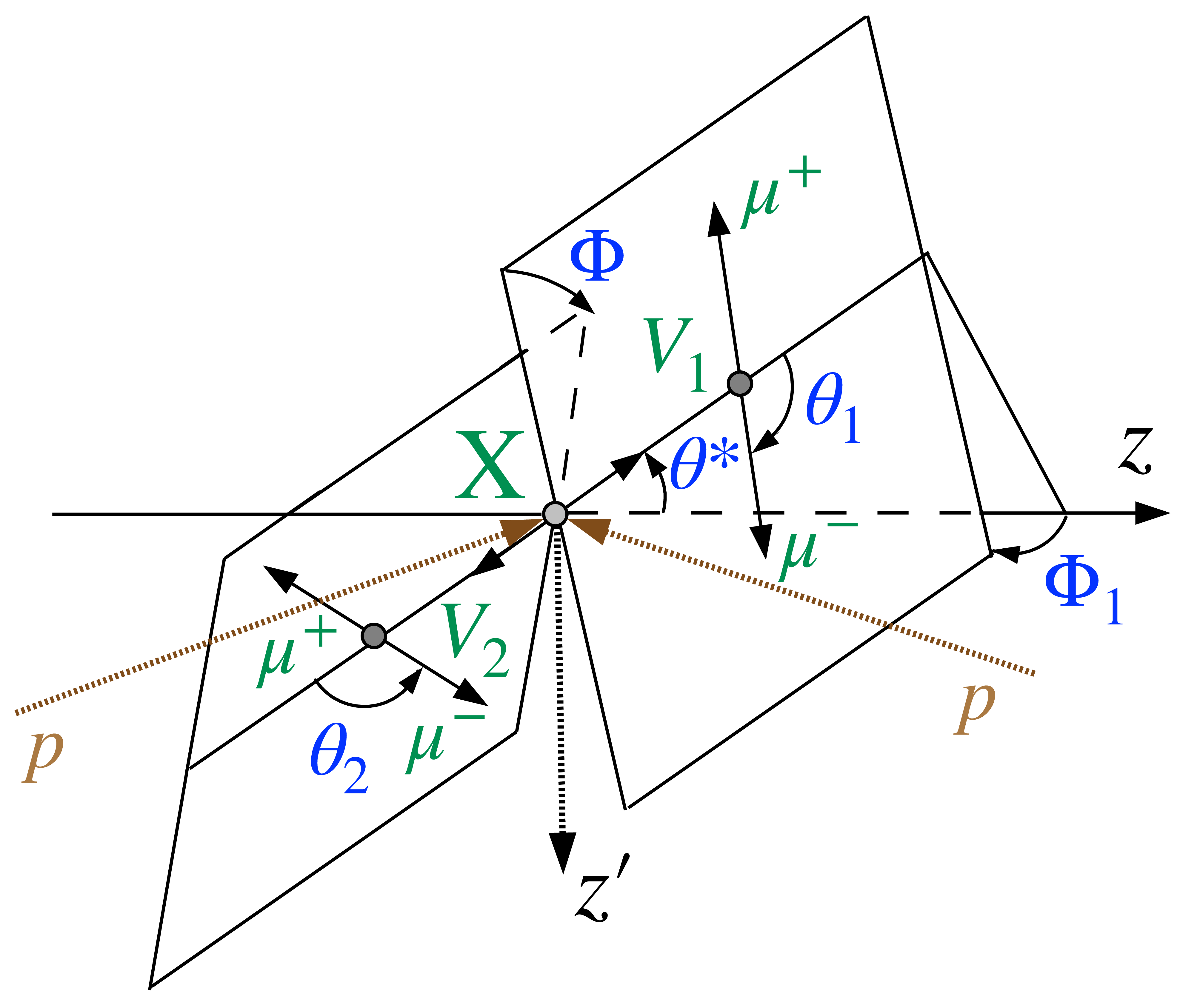
Angular observables. The production and decay of a resonance $ \mathrm{X} $ in proton collisions $ \mathrm{p}\mathrm{p}\to \mathrm{X} \to \mathrm{V}_1\mathrm{V}_2 \to 4\mu $ define the angular observables in the centre-of-mass frames of the corresponding particles [46, 35], where the $ \mathrm{V}_1 $ and $ \mathrm{V}_2 $ refer to the $ \mathrm{J}/\psi $ mesons. The $ z $ axis approximates the proton beam line, while the $ z' $ axis corresponds to the direction of the four-muon system. |
png pdf |
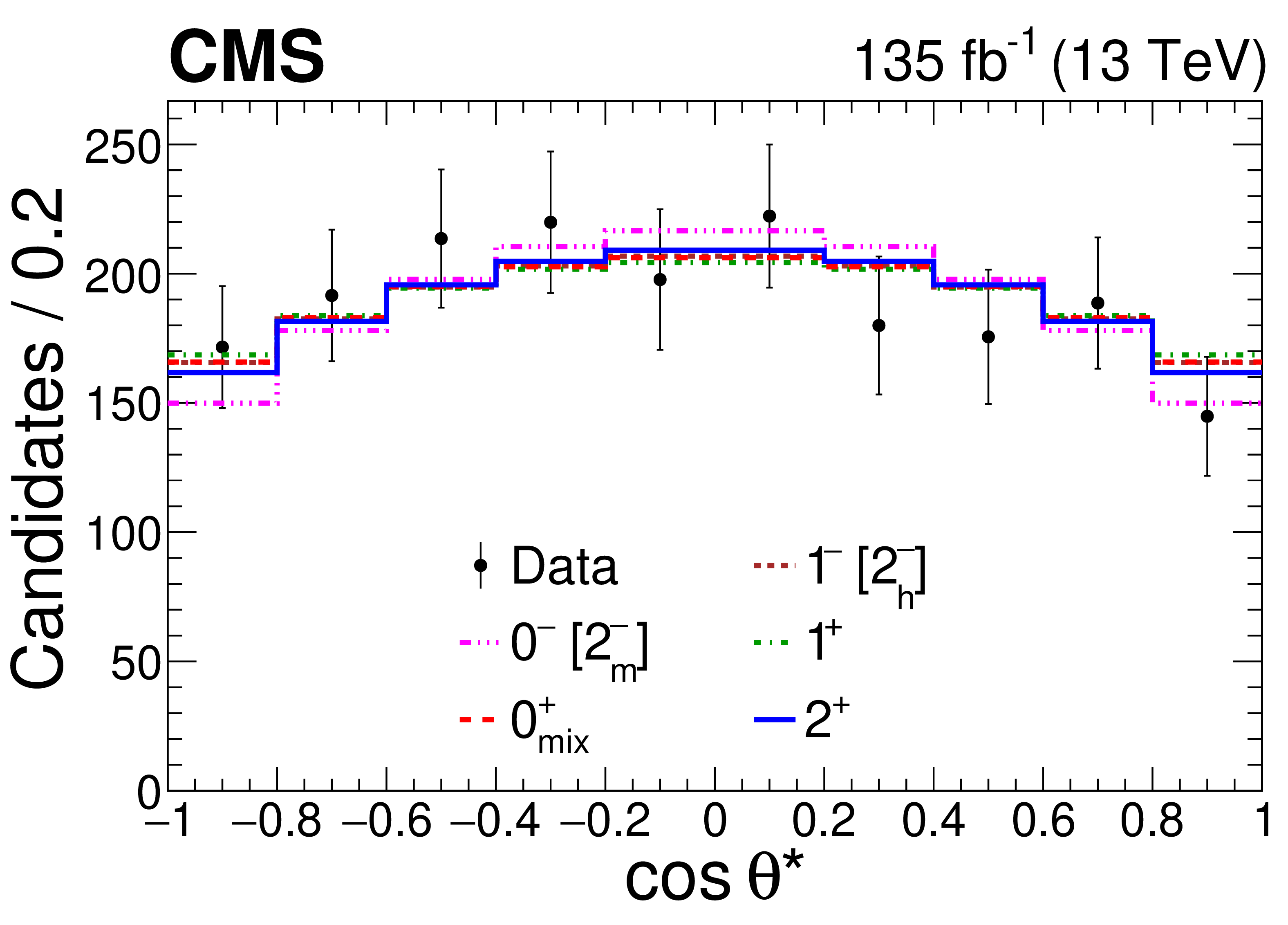
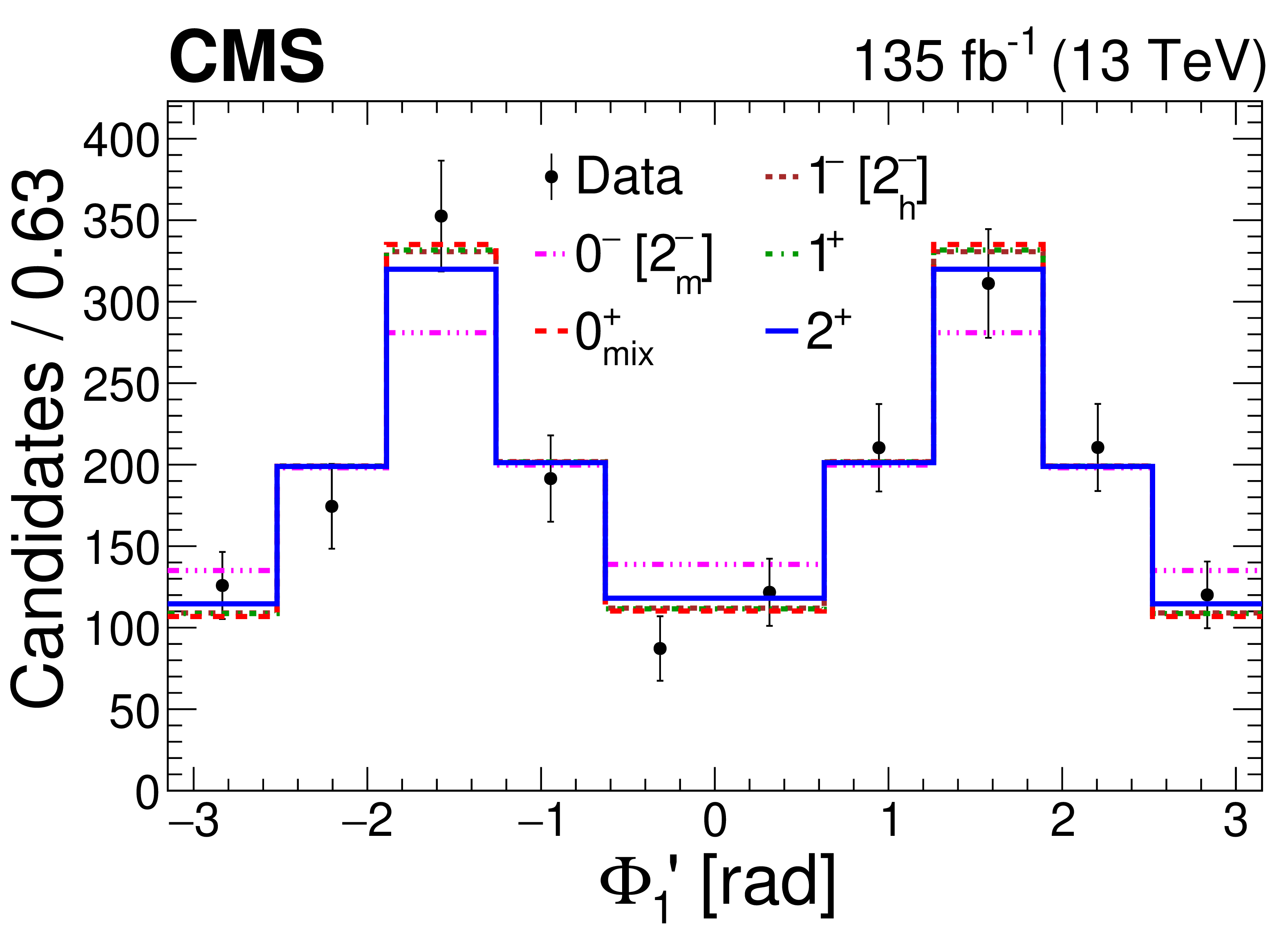
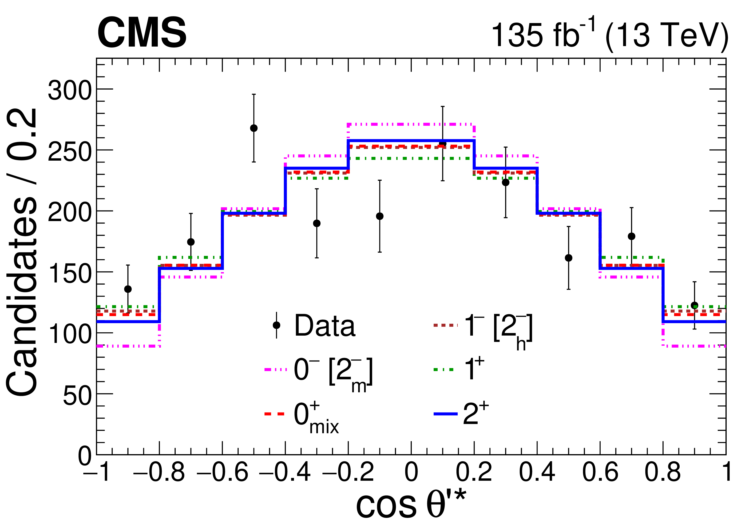
Figure 6:
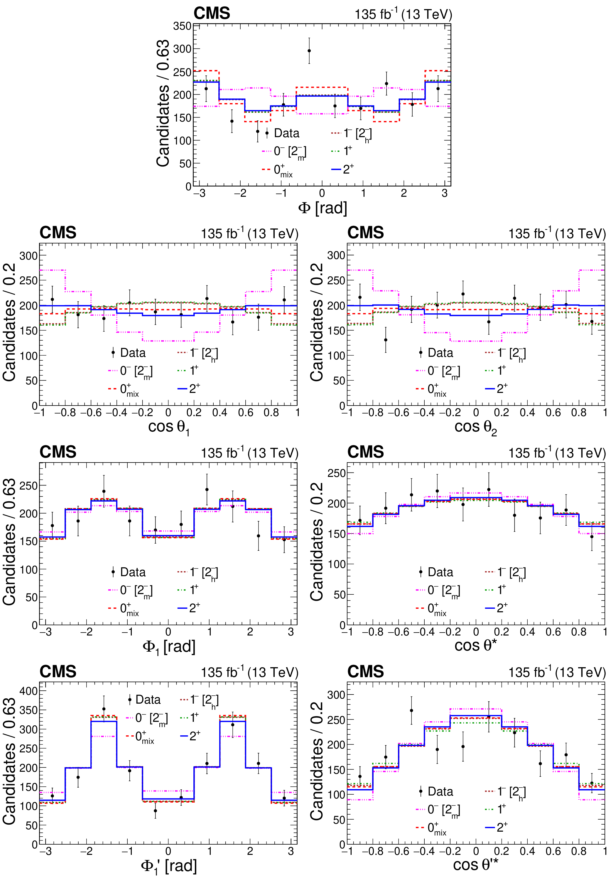
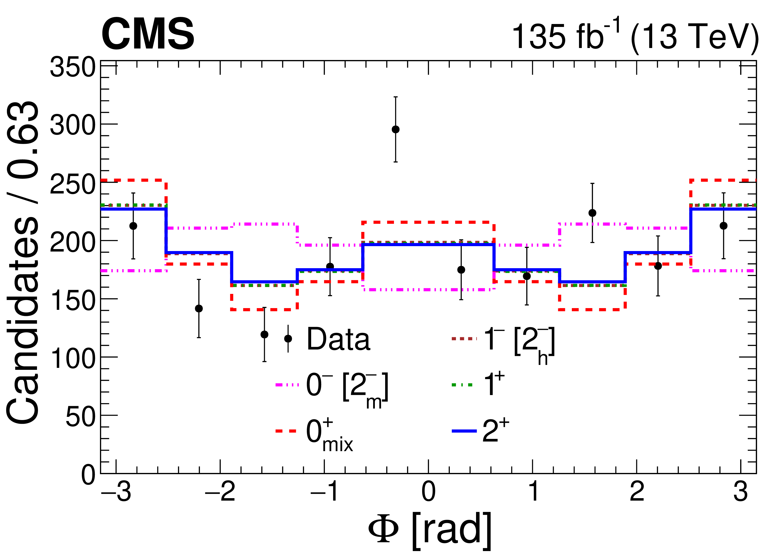
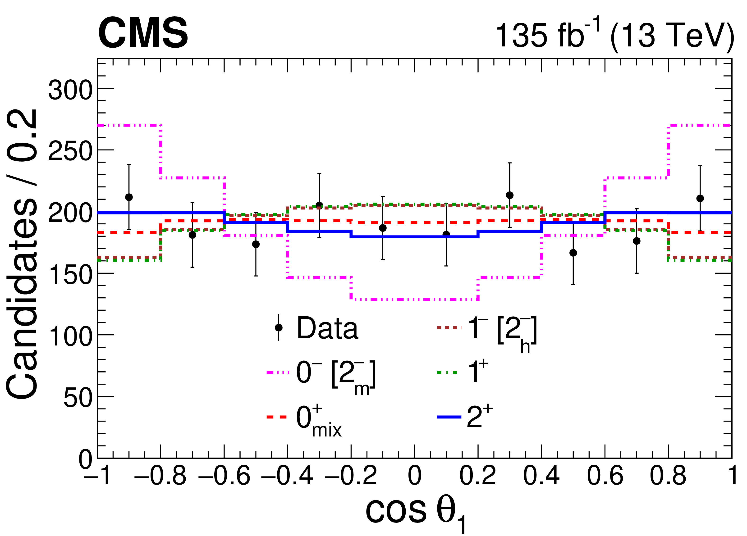
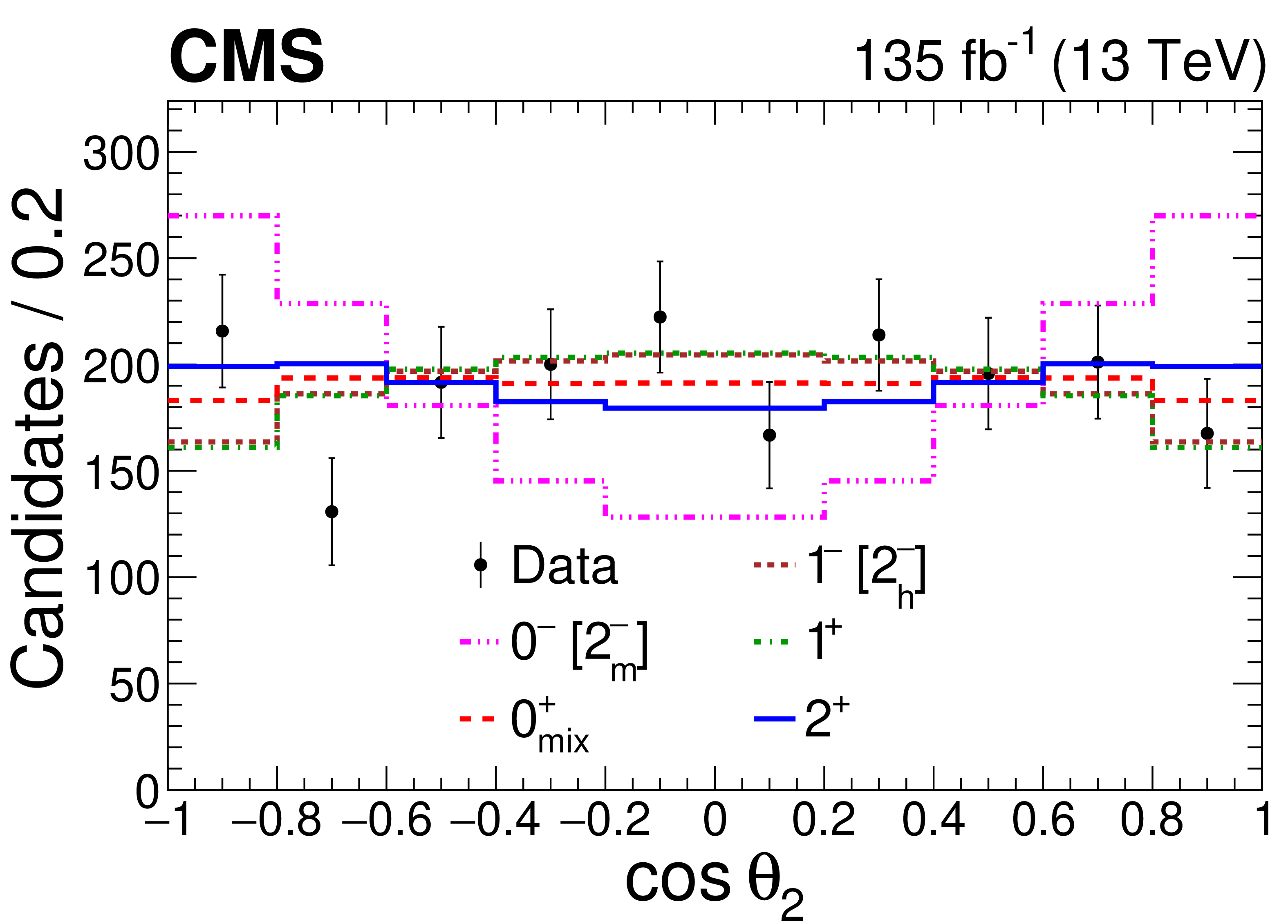
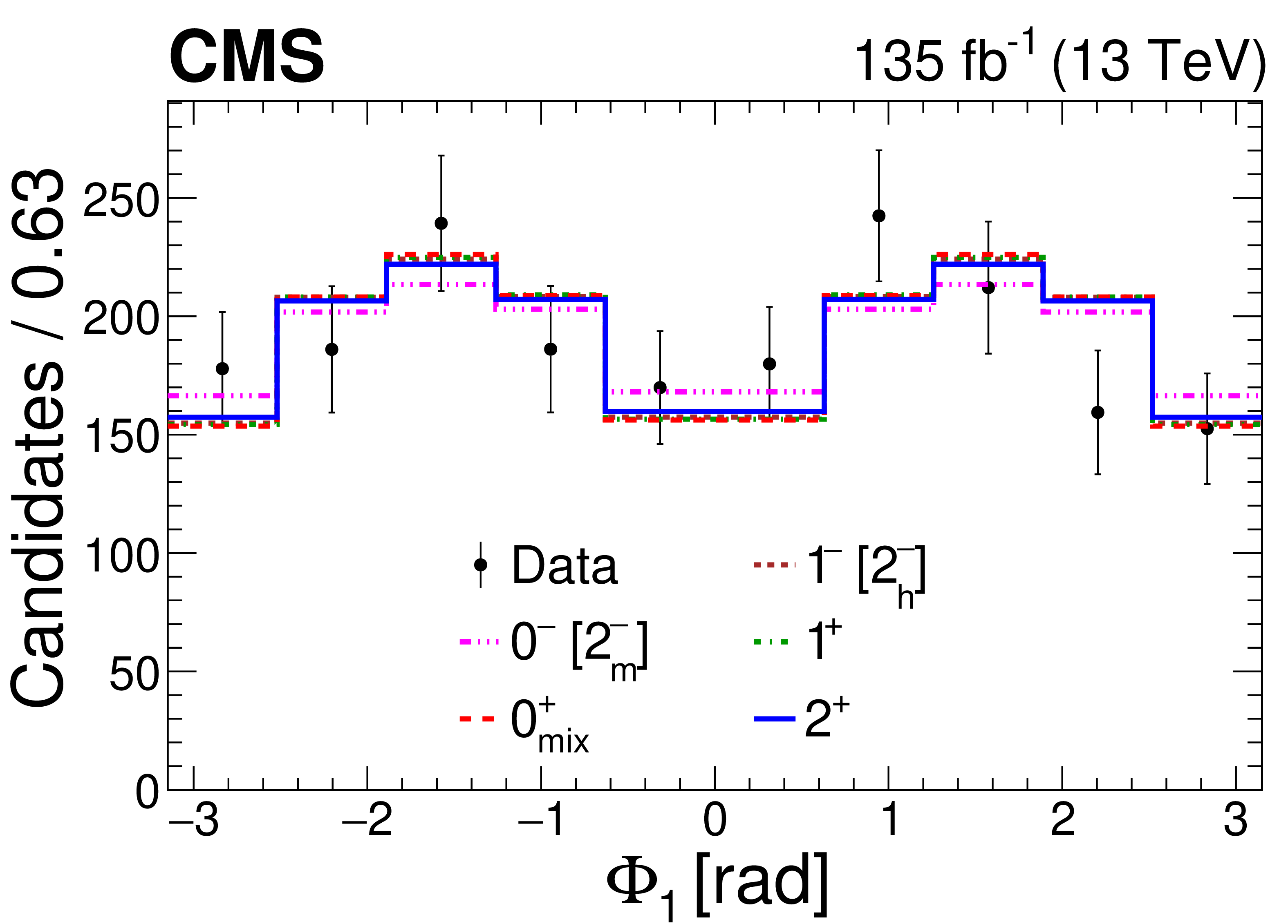
Angular distributions. Distribution of the decay angles: $ \Phi $ (upper row), $ \cos\theta_1, \cos\theta_2 $ (second row), production angles defined with respect to axis $ z $: $ \Phi_1, \cos\theta^* $ (third row), and defined with respect to axis $ z' $: $ \Phi_1', \cos\theta^{\prime *} $ (lower row) in the range 6.2 $ < m_{4\mu} < $ 8.0 GeV presented together with the five $ J^P_i $ signal models. The background is subtracted from the data, based on the expected distributions, and systematic uncertainties are not incorporated in these plots. The $ 0^{-} $ and 2 $ _m^{-} $ distributions are identical, as are those of $ 1^{-} $ and 2 $ _h^{-} $. |
png pdf |
Figure 6-a:
Angular distributions. Distribution of the decay angles: $ \Phi $ (upper row), $ \cos\theta_1, \cos\theta_2 $ (second row), production angles defined with respect to axis $ z $: $ \Phi_1, \cos\theta^* $ (third row), and defined with respect to axis $ z' $: $ \Phi_1', \cos\theta^{\prime *} $ (lower row) in the range 6.2 $ < m_{4\mu} < $ 8.0 GeV presented together with the five $ J^P_i $ signal models. The background is subtracted from the data, based on the expected distributions, and systematic uncertainties are not incorporated in these plots. The $ 0^{-} $ and 2 $ _m^{-} $ distributions are identical, as are those of $ 1^{-} $ and 2 $ _h^{-} $. |
png pdf |
Figure 6-b:
Angular distributions. Distribution of the decay angles: $ \Phi $ (upper row), $ \cos\theta_1, \cos\theta_2 $ (second row), production angles defined with respect to axis $ z $: $ \Phi_1, \cos\theta^* $ (third row), and defined with respect to axis $ z' $: $ \Phi_1', \cos\theta^{\prime *} $ (lower row) in the range 6.2 $ < m_{4\mu} < $ 8.0 GeV presented together with the five $ J^P_i $ signal models. The background is subtracted from the data, based on the expected distributions, and systematic uncertainties are not incorporated in these plots. The $ 0^{-} $ and 2 $ _m^{-} $ distributions are identical, as are those of $ 1^{-} $ and 2 $ _h^{-} $. |
png pdf |
Figure 6-c:
Angular distributions. Distribution of the decay angles: $ \Phi $ (upper row), $ \cos\theta_1, \cos\theta_2 $ (second row), production angles defined with respect to axis $ z $: $ \Phi_1, \cos\theta^* $ (third row), and defined with respect to axis $ z' $: $ \Phi_1', \cos\theta^{\prime *} $ (lower row) in the range 6.2 $ < m_{4\mu} < $ 8.0 GeV presented together with the five $ J^P_i $ signal models. The background is subtracted from the data, based on the expected distributions, and systematic uncertainties are not incorporated in these plots. The $ 0^{-} $ and 2 $ _m^{-} $ distributions are identical, as are those of $ 1^{-} $ and 2 $ _h^{-} $. |
png pdf |
Figure 6-d:
Angular distributions. Distribution of the decay angles: $ \Phi $ (upper row), $ \cos\theta_1, \cos\theta_2 $ (second row), production angles defined with respect to axis $ z $: $ \Phi_1, \cos\theta^* $ (third row), and defined with respect to axis $ z' $: $ \Phi_1', \cos\theta^{\prime *} $ (lower row) in the range 6.2 $ < m_{4\mu} < $ 8.0 GeV presented together with the five $ J^P_i $ signal models. The background is subtracted from the data, based on the expected distributions, and systematic uncertainties are not incorporated in these plots. The $ 0^{-} $ and 2 $ _m^{-} $ distributions are identical, as are those of $ 1^{-} $ and 2 $ _h^{-} $. |
png pdf |
Figure 6-e:
Angular distributions. Distribution of the decay angles: $ \Phi $ (upper row), $ \cos\theta_1, \cos\theta_2 $ (second row), production angles defined with respect to axis $ z $: $ \Phi_1, \cos\theta^* $ (third row), and defined with respect to axis $ z' $: $ \Phi_1', \cos\theta^{\prime *} $ (lower row) in the range 6.2 $ < m_{4\mu} < $ 8.0 GeV presented together with the five $ J^P_i $ signal models. The background is subtracted from the data, based on the expected distributions, and systematic uncertainties are not incorporated in these plots. The $ 0^{-} $ and 2 $ _m^{-} $ distributions are identical, as are those of $ 1^{-} $ and 2 $ _h^{-} $. |
png pdf |
Figure 6-f:
Angular distributions. Distribution of the decay angles: $ \Phi $ (upper row), $ \cos\theta_1, \cos\theta_2 $ (second row), production angles defined with respect to axis $ z $: $ \Phi_1, \cos\theta^* $ (third row), and defined with respect to axis $ z' $: $ \Phi_1', \cos\theta^{\prime *} $ (lower row) in the range 6.2 $ < m_{4\mu} < $ 8.0 GeV presented together with the five $ J^P_i $ signal models. The background is subtracted from the data, based on the expected distributions, and systematic uncertainties are not incorporated in these plots. The $ 0^{-} $ and 2 $ _m^{-} $ distributions are identical, as are those of $ 1^{-} $ and 2 $ _h^{-} $. |
png pdf |
Figure 6-g:
Angular distributions. Distribution of the decay angles: $ \Phi $ (upper row), $ \cos\theta_1, \cos\theta_2 $ (second row), production angles defined with respect to axis $ z $: $ \Phi_1, \cos\theta^* $ (third row), and defined with respect to axis $ z' $: $ \Phi_1', \cos\theta^{\prime *} $ (lower row) in the range 6.2 $ < m_{4\mu} < $ 8.0 GeV presented together with the five $ J^P_i $ signal models. The background is subtracted from the data, based on the expected distributions, and systematic uncertainties are not incorporated in these plots. The $ 0^{-} $ and 2 $ _m^{-} $ distributions are identical, as are those of $ 1^{-} $ and 2 $ _h^{-} $. |
png pdf |
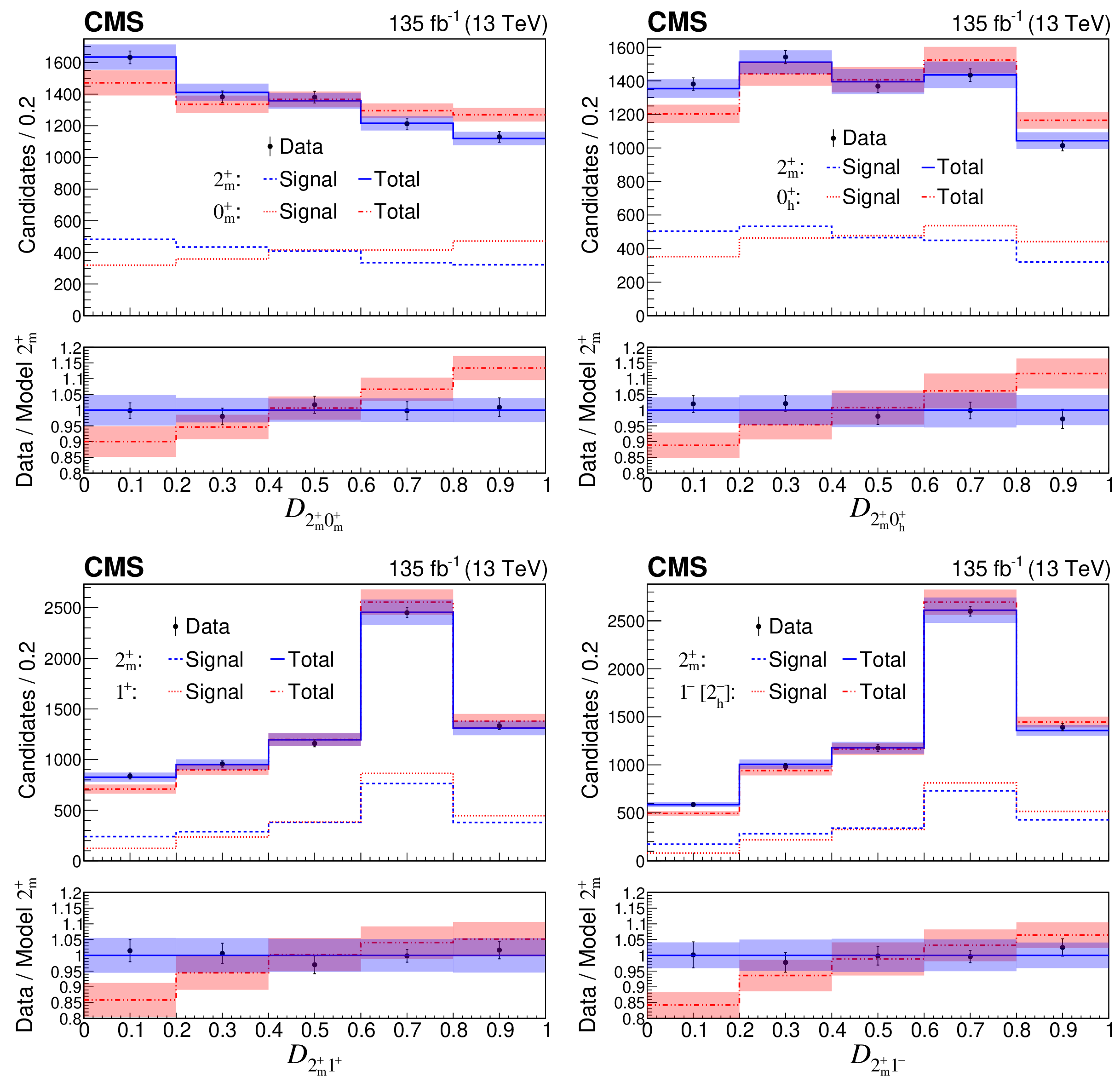
Figure 7:
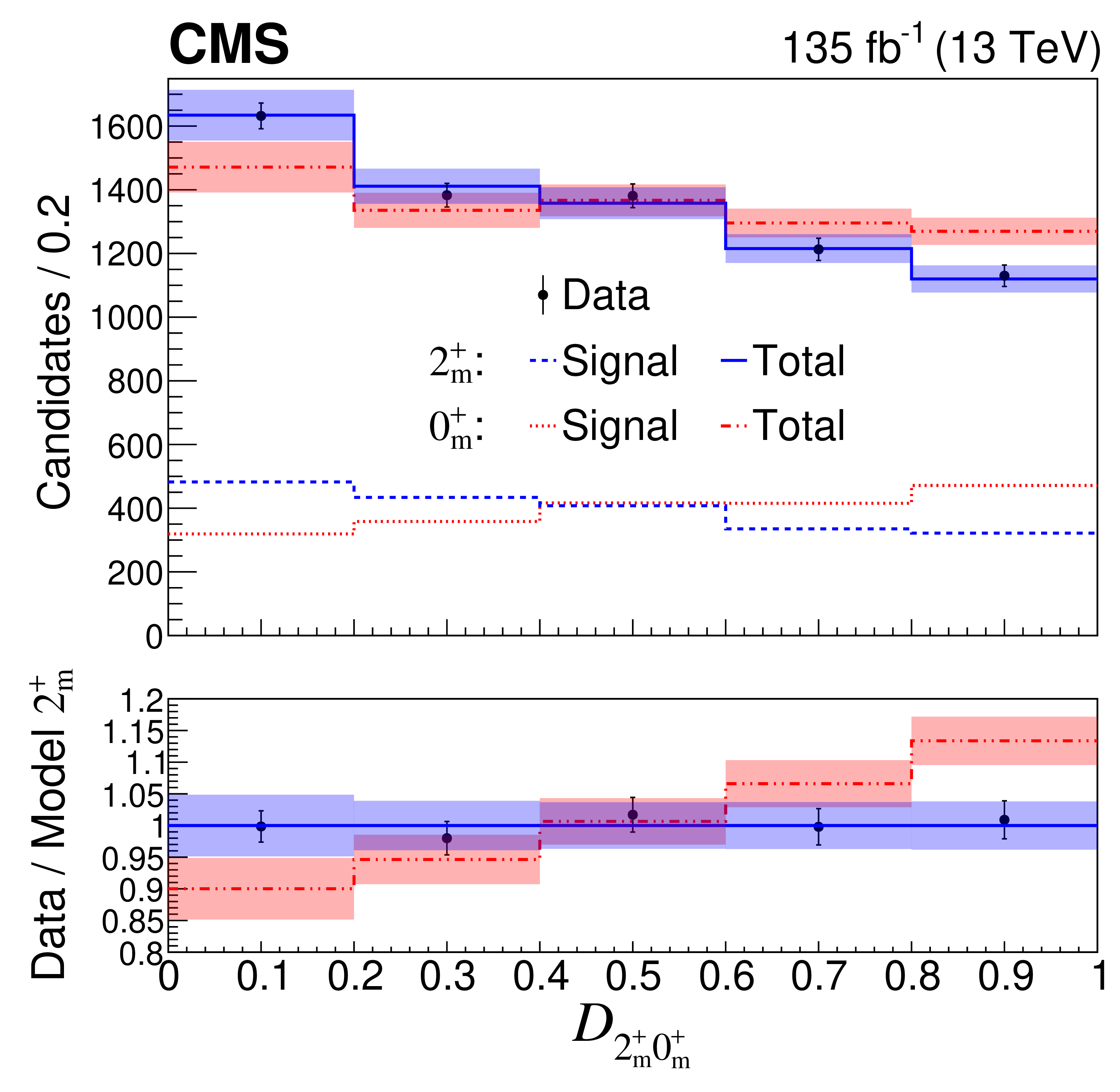
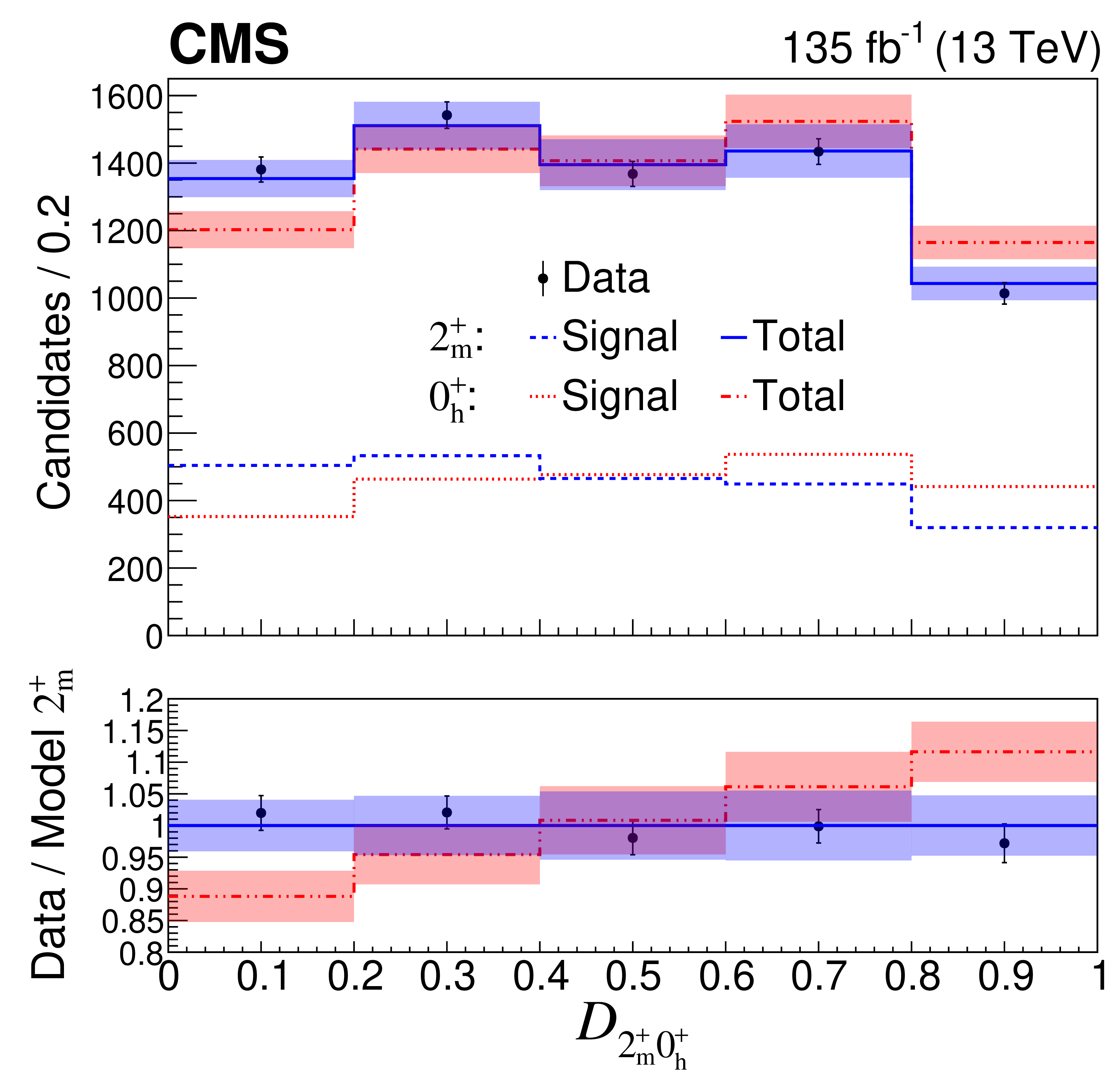
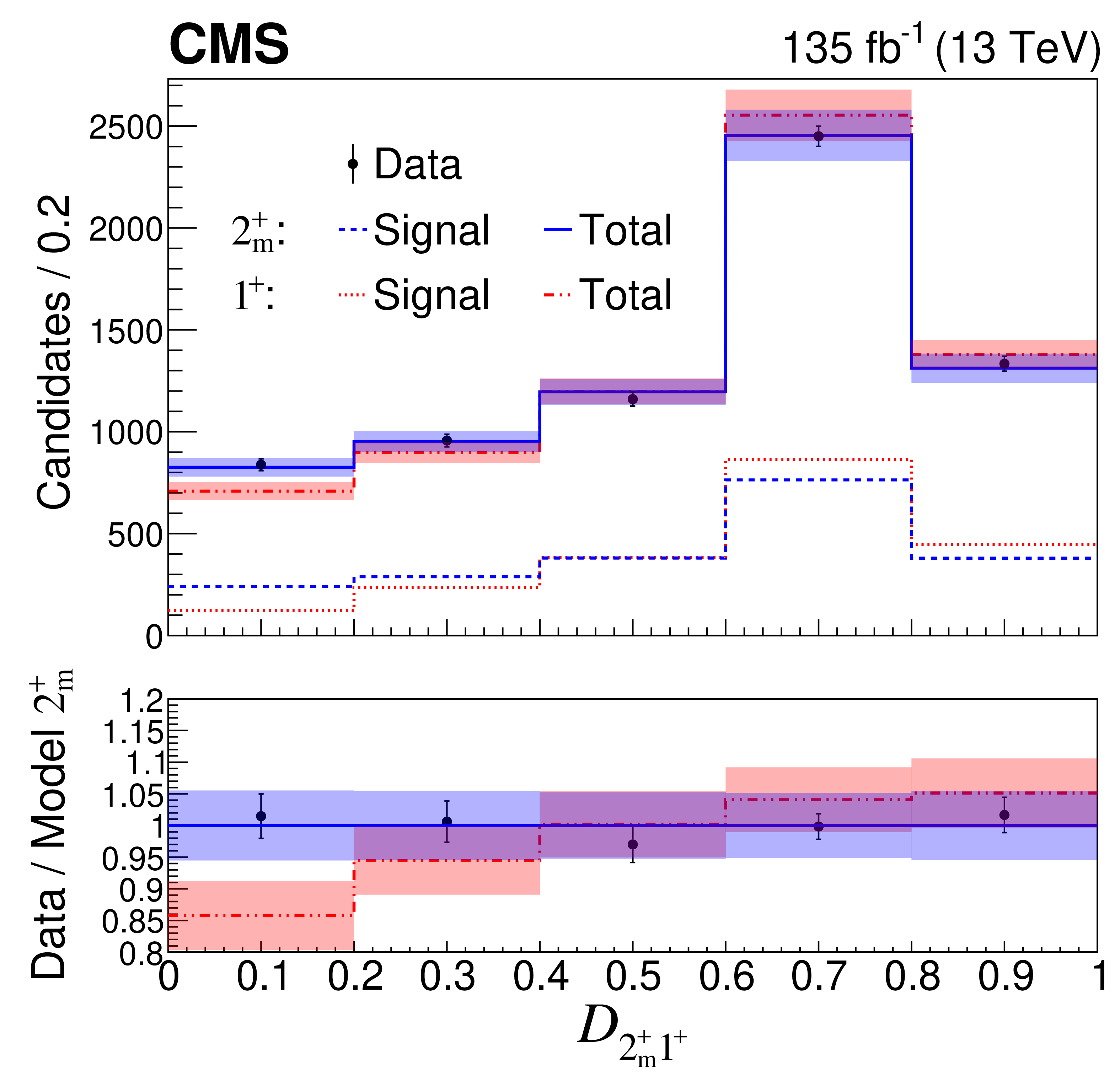
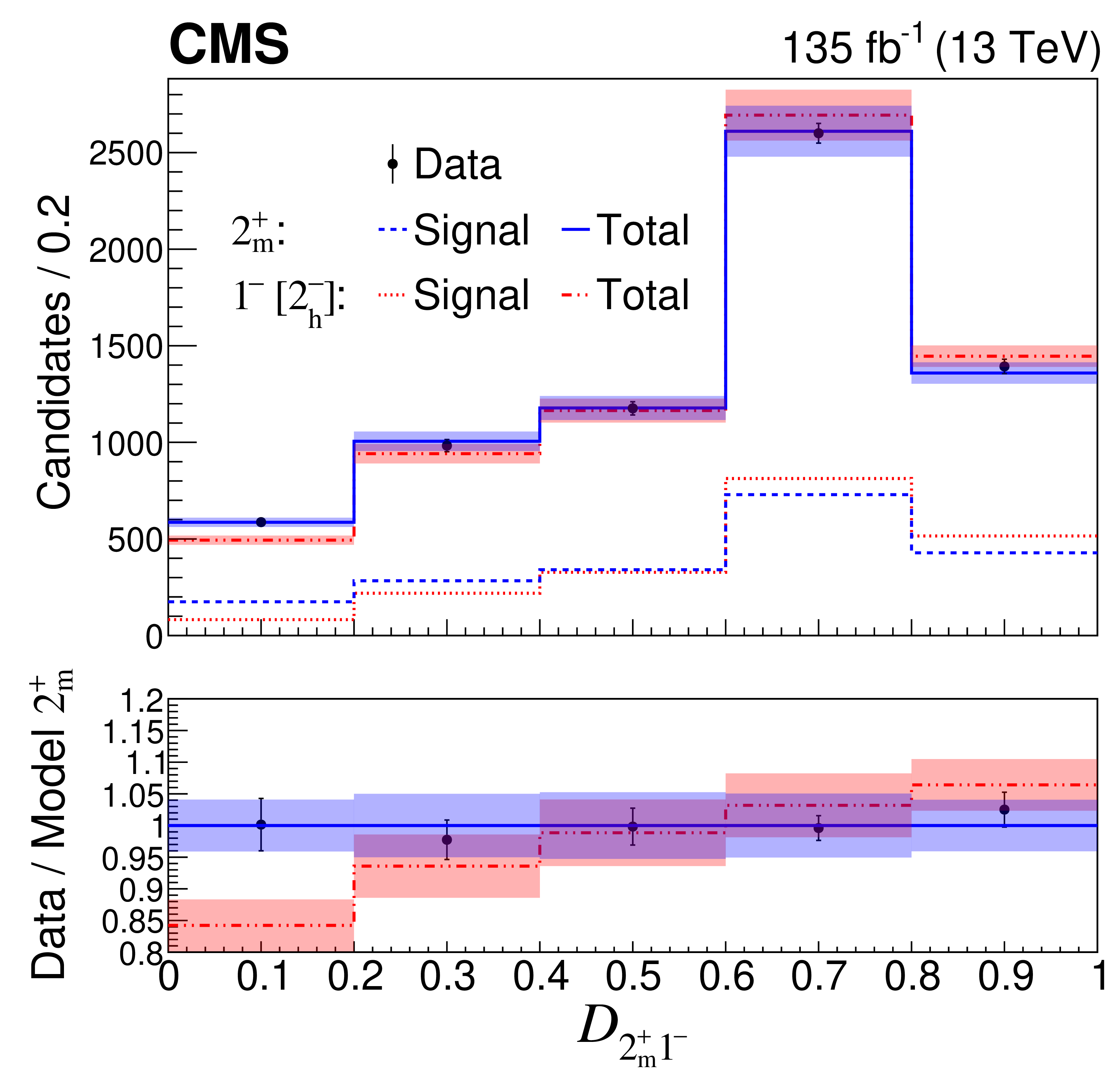
Optimal observables. Distributions of $ \mathcal{D}_{ij} $ that are optimal for separating the 2 $ _{m}^+ $ model against the 0 $ _{m}^+ $ (upper left), 0 $ _{h}^+ $ (upper right), $ 1^- $ (lower left), and $ 1^+ $ (lower right) models in the range 6.2 $ < m_{4\mu} < $ 8.0 GeV. Distributions for signal only (dashed) and for signal plus background (solid and dash-dot-dotted) models are compared to the experimental data points with error bars, with uncertainty bands representing post-fit model uncertainties, which are partially correlated with the data. The $ 1^{-} $ and 2 $ _h^{-} $ distributions are identical, apart from systematic uncertainties arising from polarization effects. The lower panels display the ratios of the data and of the model predictions to the mean expectations from the 2 $ _{m}^+ $ model. |
png pdf |
Figure 7-a:
Optimal observables. Distributions of $ \mathcal{D}_{ij} $ that are optimal for separating the 2 $ _{m}^+ $ model against the 0 $ _{m}^+ $ (upper left), 0 $ _{h}^+ $ (upper right), $ 1^- $ (lower left), and $ 1^+ $ (lower right) models in the range 6.2 $ < m_{4\mu} < $ 8.0 GeV. Distributions for signal only (dashed) and for signal plus background (solid and dash-dot-dotted) models are compared to the experimental data points with error bars, with uncertainty bands representing post-fit model uncertainties, which are partially correlated with the data. The $ 1^{-} $ and 2 $ _h^{-} $ distributions are identical, apart from systematic uncertainties arising from polarization effects. The lower panels display the ratios of the data and of the model predictions to the mean expectations from the 2 $ _{m}^+ $ model. |
png pdf |
Figure 7-b:
Optimal observables. Distributions of $ \mathcal{D}_{ij} $ that are optimal for separating the 2 $ _{m}^+ $ model against the 0 $ _{m}^+ $ (upper left), 0 $ _{h}^+ $ (upper right), $ 1^- $ (lower left), and $ 1^+ $ (lower right) models in the range 6.2 $ < m_{4\mu} < $ 8.0 GeV. Distributions for signal only (dashed) and for signal plus background (solid and dash-dot-dotted) models are compared to the experimental data points with error bars, with uncertainty bands representing post-fit model uncertainties, which are partially correlated with the data. The $ 1^{-} $ and 2 $ _h^{-} $ distributions are identical, apart from systematic uncertainties arising from polarization effects. The lower panels display the ratios of the data and of the model predictions to the mean expectations from the 2 $ _{m}^+ $ model. |
png pdf |
Figure 7-c:
Optimal observables. Distributions of $ \mathcal{D}_{ij} $ that are optimal for separating the 2 $ _{m}^+ $ model against the 0 $ _{m}^+ $ (upper left), 0 $ _{h}^+ $ (upper right), $ 1^- $ (lower left), and $ 1^+ $ (lower right) models in the range 6.2 $ < m_{4\mu} < $ 8.0 GeV. Distributions for signal only (dashed) and for signal plus background (solid and dash-dot-dotted) models are compared to the experimental data points with error bars, with uncertainty bands representing post-fit model uncertainties, which are partially correlated with the data. The $ 1^{-} $ and 2 $ _h^{-} $ distributions are identical, apart from systematic uncertainties arising from polarization effects. The lower panels display the ratios of the data and of the model predictions to the mean expectations from the 2 $ _{m}^+ $ model. |
png pdf |
Figure 7-d:
Optimal observables. Distributions of $ \mathcal{D}_{ij} $ that are optimal for separating the 2 $ _{m}^+ $ model against the 0 $ _{m}^+ $ (upper left), 0 $ _{h}^+ $ (upper right), $ 1^- $ (lower left), and $ 1^+ $ (lower right) models in the range 6.2 $ < m_{4\mu} < $ 8.0 GeV. Distributions for signal only (dashed) and for signal plus background (solid and dash-dot-dotted) models are compared to the experimental data points with error bars, with uncertainty bands representing post-fit model uncertainties, which are partially correlated with the data. The $ 1^{-} $ and 2 $ _h^{-} $ distributions are identical, apart from systematic uncertainties arising from polarization effects. The lower panels display the ratios of the data and of the model predictions to the mean expectations from the 2 $ _{m}^+ $ model. |
| Tables | |
png pdf |
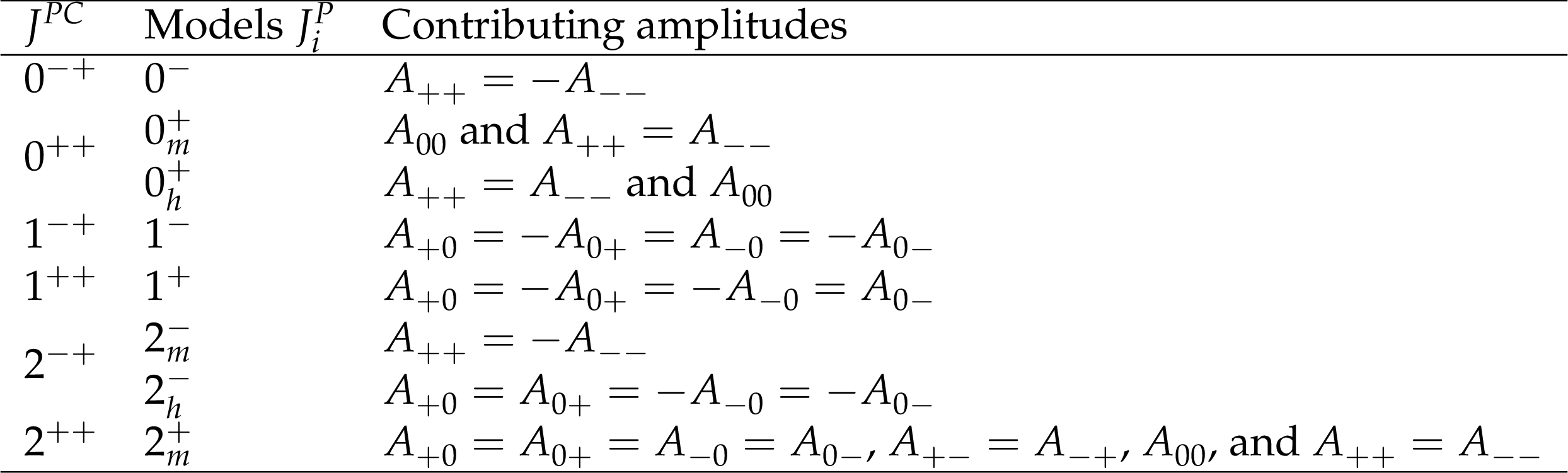
Table 1:
Quantum numbers. The possible assignments of quantum numbers $ J^{PC} $, the $ J_i^{P} $ models considered, and the contributing amplitudes in the decay $ \mathrm{X}\to \mathrm{J}/\psi \mathrm{J}/\psi $ are presented. |
png pdf |
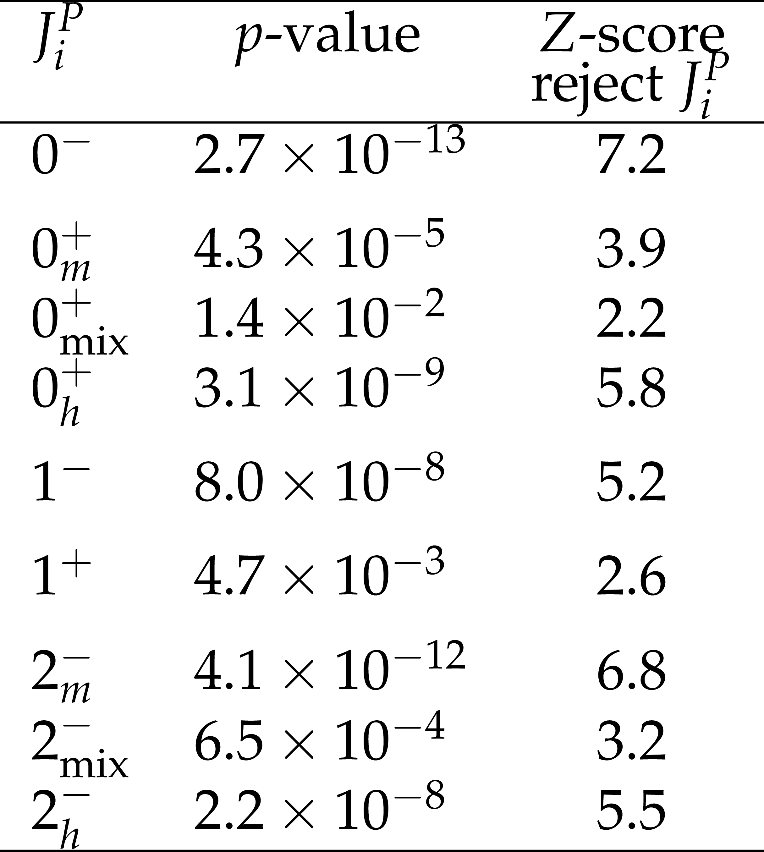
Table 2:
Summary of statistical tests. The $ p $-value and the associated $ Z $-score are shown for alternative models $ J_i^{P} $, tested against the 2 $ _m^{+} $ model. A higher Z-score implies that the model is less compatible with observation. |

png pdf |
Table 3:
Results from hypothesis test for pairs of spin-parity models. This is an extended version of Table 2. The expected $ p $-value is presented based on the assumption of the scenario of 2 $ _m^+ $. Results with $ Z > $ 5 have been derived through Gaussian extrapolation. |
| Summary |
| The study of tetraquark states has attracted considerable interest due to its potential to provide insight into the structure of the hadronic matter that makes up the world around us [4, 5, 6, 7, 8, 8, 9, 10, 11, 12, 13, 14, 15, 16, 17, 18, 19, 20, 21, 22, 23, 24, 25, 26, 27, 28, 29]. In this paper, we have presented the first measurement of the quantum numbers for a recently discovered family of three all-charm tetraquarks, based on data collected by the CMS experiment at the LHC. Our results, summarized in Table 2, favour a $ J^{PC}=$ 2$^{++} $ assignment. For a system of two constituents, as represented by either model in Fig. 2, an orbital angular momentum of $ L = $ 1 is excluded by the requirement $ P = + $1, while higher orbital excitations with $ L \geq $ 2 are energetically disfavoured. This makes the $ S $-wave ($ L = $ 0) configuration the most likely. In a molecular scenario, the quark-antiquark pairs are not required to be spin-1 mesons, making a $ J = $ 2 configuration less likely. This picture agreed with existing data for all other well-established tetraquark candidates with measured spin, such as the X(3872) and $ \mathrm{Z}_{\mathrm{c}}(3900)^{+} $, all of which have $ J < $ 2 [3]. In contrast, a tightly-bound $ \mathrm{c}\mathrm{c}\overline{\mathrm{c}}\overline{\mathrm{c}} $ tetraquark with a diquark--antidiquark configuration requires both diquarks to be in spin-1 states, which restricts the total spin to $ J = $ 0 or $ J = $ 2, making $ J = $ 2 a natural choice. This spin-1 diquark requirement, however, does not apply to tetraquark candidates with mixed-flavour quark content, a consideration relevant to all previously observed candidates, which contained both heavy and light quarks [3]. Other theoretical considerations also favour $ J = $ 2 for the tightly-bound tetraquark states [18, 28]. This advancement in understanding exotic hadrons was enabled by the study of all-heavy tetraquarks and it brings us closer to uncovering their internal structure. Although our findings do not definitively distinguish between tightly-bound tetraquark and meson-meson molecular models, they provide constraints on the possible internal structures and favour the tightly-bound scenario. |
| References | ||||
| 1 | M. Gell-Mann | A schematic model of baryons and mesons | PL 8 (1964) 214 | |
| 2 | G. Zweig | An SU(3) model for strong interaction symmetry and its breaking. Version 2 | CERN 2 (1964) 2 | |
| 3 | Particle Data Group | Review of particle physics | PRD 110 (2024) 030001 | |
| 4 | A. V. Berezhnoy, A. V. Luchinsky, and A. A. Novoselov | Heavy tetraquarks production at the LHC | PRD 86 (2012) 034004 | 1111.1867 |
| 5 | J. Wu et al. | Heavy-flavored tetraquark states with the $ QQ\bar{Q}\bar{Q} $ configuration | PRD 97 (2018) 094015 | 1605.01134 |
| 6 | M. Karliner, S. Nussinov, and J. L. Rosner | $ QQ\bar{Q}\bar{Q} $ states: Masses, production, and decays | PRD 95 (2017) 034011 | 1611.00348 |
| 7 | J.-M. Richard, A. Valcarce, and J. Vijande | String dynamics and metastability of all-heavy tetraquarks | PRD 95 (2017) 054019 | 1703.00783 |
| 8 | M. N. Anwar et al. | Spectroscopy and decays of the fully-heavy tetraquarks | EPJC 78 (2018) 647 | 1710.02540 |
| 9 | M. Nielsen et al. | Supersymmetry in the double-heavy hadronic spectrum | PRD 98 (2018) 034002 | 1805.11567 |
| 10 | M. Nielsen and S. J. Brodsky | Hadronic superpartners from a superconformal and supersymmetric algebra | PRD 97 (2018) 114001 | 1802.09652 |
| 11 | A. Ali, L. Maiani, and A. D. Polosa | Multiquark hadrons | Cambridge University Press, ISBN 978-1-316-76146-5, 2019 link |
|
| 12 | N. Brambilla et al. | The XYZ states: experimental and theoretical status and perspectives | Phys. Rept. 873 (2020) 1 | 1907.07583 |
| 13 | M.-S. Liu, Q.-F. Lu, X.-H. Zhong, and Q. Zhao | All-heavy tetraquarks | PRD 100 (2019) 016006 | 1901.02564 |
| 14 | G.-J. Wang, L. Meng, and S.-L. Zhu | Spectrum of the fully-heavy tetraquark state $ QQ\bar Q' \bar Q' $ | PRD 100 (2019) 096013 | 1907.05177 |
| 15 | M. A. Bedolla, J. Ferretti, C. D. Roberts, and E. Santopinto | Spectrum of fully-heavy tetraquarks from a diquark+antidiquark perspective | EPJC 80 (2020) 1004 | 1911.00960 |
| 16 | M.-S. Liu, F.-X. Liu, X.-H. Zhong, and Q. Zhao | Fully heavy tetraquark states and their evidences in LHC observations | PRD 109 (2024) 076017 | 2006.11952 |
| 17 | X. Jin, Y. Xue, H. Huang, and J. Ping | Full-heavy tetraquarks in constituent quark models | EPJC 80 (2020) 1083 | 2006.13745 |
| 18 | C. Becchi et al. | A study of $ \mathrm{c c\bar{c}\bar{c}} $ tetraquark decays in 4 muons and in $ \mathrm{D}^{(*)} \bar{\mathrm{D}}^{(*)} $ at LHC | PLB 811 (2020) 135952 | 2006.14388 |
| 19 | H.-X. Chen, W. Chen, X. Liu, and S.-L. Zhu | Strong decays of fully-charm tetraquarks into di-charmonia | Sci. Bull. 65 (2020) 1994 | 2006.16027 |
| 20 | J.-Z. Wang, D.-Y. Chen, X. Liu, and T. Matsuki | Producing fully charm structures in the $ \mathrm{J}/\psi $-pair invariant mass spectrum | PRD 103 (2021) 071503 | 2008.07430 |
| 21 | X.-K. Dong at al. | none | ||
| 22 | H.-F. Zhang, Y.-Q. Ma, and W.-L. Sang | Perturbative QCD evidence for spin-2 particles in the di-J/$\psi$ resonances | Sci. Bull. 70 (2025) 1915 | 2009.08376 |
| 23 | R. Zhu | Fully-heavy tetraquark spectra and production at hadron colliders | NPB 966 (2021) 115393 | 2010.09082 |
| 24 | F.-X. Liu, M.-S. Liu, X.-H. Zhong, and Q. Zhao | Higher mass spectra of the fully-charmed and fully-bottom tetraquarks | PRD 104 (2021) 116029 | 2110.09052 |
| 25 | R. N. Faustov, V. O. Galkin, and E. M. Savchenko | Fully heavy tetraquark spectroscopy in the relativistic quark model | Symmetry 14 (2022) 2504 | 2210.16015 |
| 26 | F. Feng et al. | Inclusive production of fully charmed tetraquarks at the LHC | PRD 108 (2023) L051501 | 2304.11142 |
| 27 | F. G. Celiberto, G. Gatto, and A. Papa | Fully charmed tetraquarks from LHC to FCC: natural stability from fragmentation | EPJC 84 (2024) 1071 | 2405.14773 |
| 28 | I. Belov, A. Giachino, and E. Santopinto | Fully charmed tetraquark production at the LHC experiments | JHEP 01 (2025) 093 | 2409.12070 |
| 29 | F. Zhu, G. Bauer, and K. Yi | Experimental road to a charming family of tetraquarks ... and beyond | Chin. Phys. Lett. 41 (2024) 111201 | 2410.11210 |
| 30 | LHCb Collaboration | Observation of structure in the $ \mathrm{J}/\psi $-pair mass spectrum | Sci. Bull. 65 (2020) 1983 | 2006.16957 |
| 31 | ATLAS Collaboration | Observation of an excess of dicharmonium events in the four-muon final state with the ATLAS detector | PRL 131 (2023) 151902 | 2304.08962 |
| 32 | CMS Collaboration | New structures in the $ \mathrm{J}/\psi\mathrm{J}/\psi $ mass spectrum in proton-proton collisions at $ \sqrt{s}= $ 13 TeV | PRL 132 (2024) 111901 | CMS-BPH-21-003 2306.07164 |
| 33 | CMS Collaboration | The CMS experiment at the CERN LHC | JINST 3 (2008) S08004 | |
| 34 | CMS Collaboration | Development of the CMS detector for the CERN LHC Run 3 | JINST 19 (2024) P05064 | CMS-PRF-21-001 2309.05466 |
| 35 | S. Bolognesi et al. | On the spin and parity of a single-produced resonance at the LHC | PRD 86 (2012) 095031 | 1208.4018 |
| 36 | CMS Collaboration | Observation of a new boson at a mass of 125 GeV with the CMS experiment at the LHC | PLB 716 (2012) 30 | CMS-HIG-12-028 1207.7235 |
| 37 | CMS Collaboration | Study of the mass and spin-parity of the Higgs boson candidate via its decays to Z boson pairs | PRL 110 (2013) 081803 | CMS-HIG-12-041 1212.6639 |
| 38 | E598 Collaboration | Experimental observation of a heavy particle $ J $ | PRL 33 (1974) 1404 | |
| 39 | SLAC-SP-017 Collaboration | Discovery of a narrow resonance in $ \mathrm{e}^+ \mathrm{e}^- $ annihilation | PRL 33 (1974) 1406 | |
| 40 | L. G. Landsberg | The search for exotic hadrons | Phys. Usp. 42 (1999) 871 | |
| 41 | Belle Collaboration | Observation of a narrow charmoniumlike state in exclusive $ {\mathrm{B}^{\pm}} \to \mathrm{K^{\pm}} \pi^{+} \pi^{-} \mathrm{J}/\psi $ decays | PRL 91 (2003) 262001 | hep-ex/0309032 |
| 42 | BESIII Collaboration | Observation of a charged charmoniumlike structure in $ \mathrm{e}^+\mathrm{e}^- \to \pi^{+}\pi^{-} \mathrm{J}/\psi $ at $ \sqrt{s}= $ 4.26 GeV | PRL 110 (2013) 252001 | 1303.5949 |
| 43 | Belle Collaboration | Study of $ \mathrm{e}^+\mathrm{e}^- \to \pi^{+} \pi^{-} \mathrm{J}/\psi $ and observation of a charged charmoniumlike state at Belle | PRL 110 (2013) 252002 | 1304.0121 |
| 44 | CMS Collaboration | HEPData record for this analysis | link | |
| 45 | H. Yukawa | On the interaction of elementary particles. I. | Proc. Phys. Math. Soc. Jap. 17 (1935) 48 | |
| 46 | Y. Gao et al. | Spin determination of single-produced resonances at hadron colliders | PRD 81 (2010) 075022 | 1001.3396 |
| 47 | L. Evans and P. Bryant (eds) | LHC machine | JINST 3 (2008) S08001 | |
| 48 | CMS Collaboration | The CMS trigger system | JINST 12 (2017) P01020 | CMS-TRG-12-001 1609.02366 |
| 49 | T. Sjostrand et al. | An introduction to PYTHIA 8.2 | Comput. Phys. Commun. 191 (2015) 159 | 1410.3012 |
| 50 | GEANT4 Collaboration | GEANT 4---a simulation toolkit | NIM A 506 (2003) 250 | |
| 51 | A. V. Gritsan et al. | New features in the JHU generator framework: constraining Higgs boson properties from on-shell and off-shell production | PRD 102 (2020) 056022 | 2002.09888 |
| 52 | CMS Collaboration | The CMS statistical analysis and combination tool: Combine | Comput. Softw. Big Sci. 8 (2024) 19 | CMS-CAT-23-001 2404.06614 |
| 53 | CMS Collaboration | Constraints on the spin-parity and anomalous HVV couplings of the Higgs boson in proton collisions at 7 and 8 TeV | PRD 92 (2015) 012004 | CMS-HIG-14-018 1411.3441 |
| 54 | T. Junk | Confidence level computation for combining searches with small statistics | NIM A 434 (1999) 435 | hep-ex/9902006 |
| 55 | A. L. Read | Presentation of search results: the $ \text{CL}_\text{s} $ technique | JPG 28 (2002) 2693 | |
|
|
Compact Muon Solenoid LHC, CERN |
|

|

|

|

|

|