CMS-PAS-SUS-17-010

CMS-PAS-SUS-17-010
Search for chargino pair production and top squark pair production in final states with two leptons in proton-proton collisions at $\sqrt{s}=$ 13 TeV
CMS Collaboration
March 2018

Abstract: A search for pair production of supersymmetric particles in events with two leptons (electrons or muons) and missing transverse momentum is reported. The data sample corresponds to 35.9 fb $^{-1}$ of proton-proton collisions at $\sqrt{s}=$ 13 TeV collected by the CMS detector during the 2016 data taking period at the CERN LHC. The search targets two signal models for chargino and top squark pair production. No significant deviation is observed from the predicted background. The results are interpreted in terms of several simplified models assuming R-parity conservation and with the neutralino as the lightest supersymmetric particle. When the chargino is assumed to undergo a cascade decay through sleptons, exclusion limits at 95% confidence level are set on the mass of the chargino up to 800 GeV and on the mass of the neutralino up to 320 GeV. For the top squark production, the search focuses on models with a small mass difference between the top squark and the lightest neutralino. When the top squark decays into an off-shell top quark and a neutralino, the limits extend up to 420 and 360 GeV for the top squark and neutralino masses, respectively.
Links: CDS record (PDF) ; inSPIRE record ; CADI line (restricted) ; These preliminary results are superseded in this paper, JHEP 11 (2018) 079. The superseded preliminary plots can be found here.

Figures & Tables	Summary	References	CMS Publications

Figures
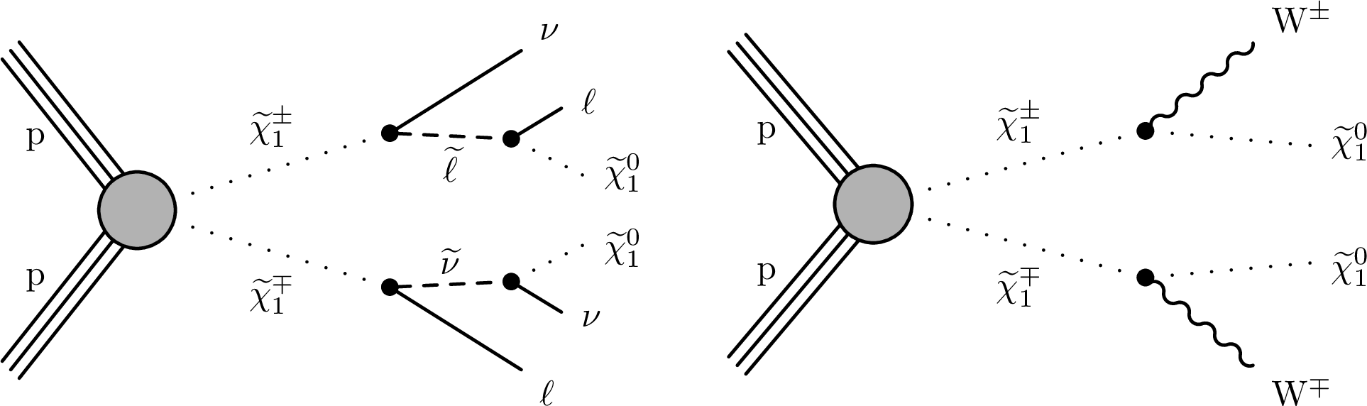
png pdf	Figure 1: Diagrams of the chargino pair production in two possible decay modes: the left plot shows decays through intermediate sleptons or sneutrinos, while the right one displays decays into a W boson and the lightest neutralino.
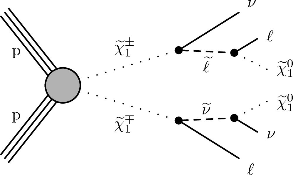
png pdf	Figure 1-a: Diagram of the chargino pair production in decay mode through intermediate sleptons or sneutrinos.
png pdf	Figure 1-b: Diagram of the chargino pair production in decay mode into a W boson and the lightest neutralino.
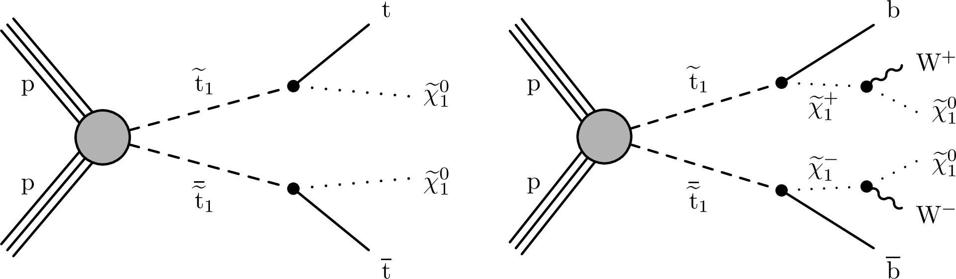
png pdf	Figure 2: Diagrams of the top squark-antisquark pair production with two possible decay modes for the top squark: the left plot shows decays into a top quark and the lightest neutralino, while the right one displays decays into a bottom quark and a chargino further decaying into a neutralino and a W boson.
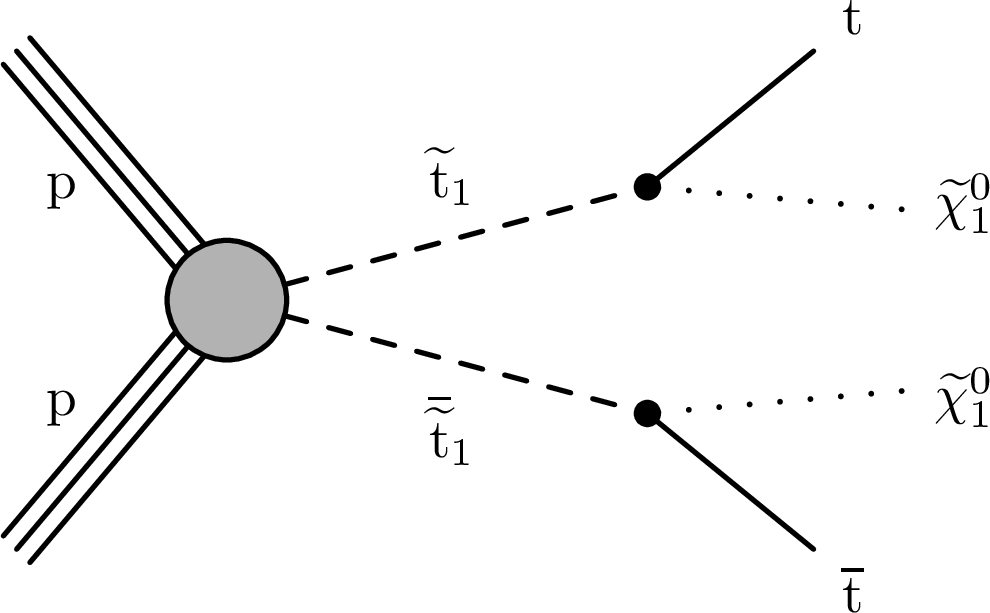
png pdf	Figure 2-a: Diagram of the top squark-antisquark pair production in top squark decay mode into a top quark and the lightest neutralino.
png pdf	Figure 2-b: Diagram of the top squark-antisquark pair production in top squark decay mode into a bottom quark and a chargino further decaying into a neutralino and a W boson.
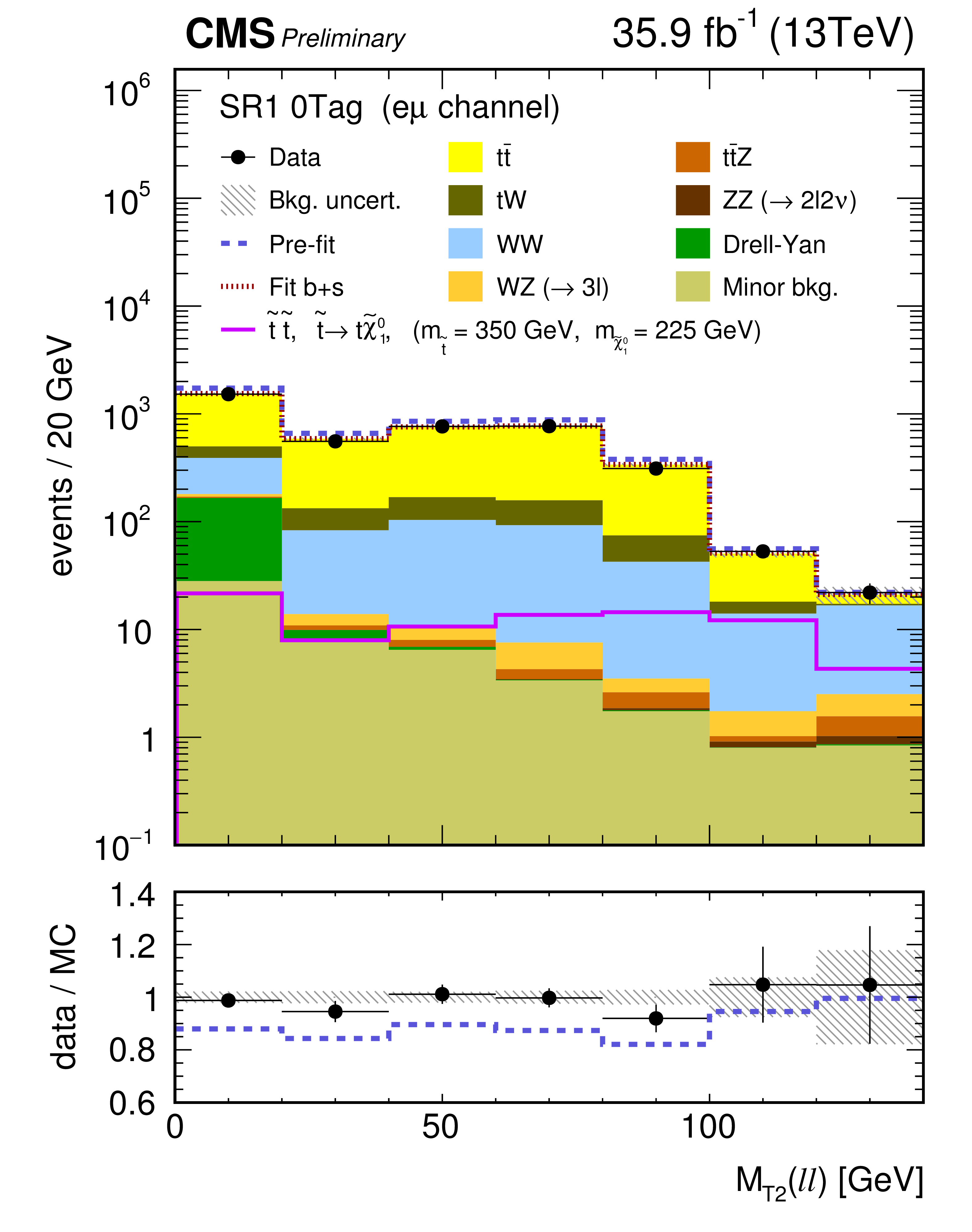
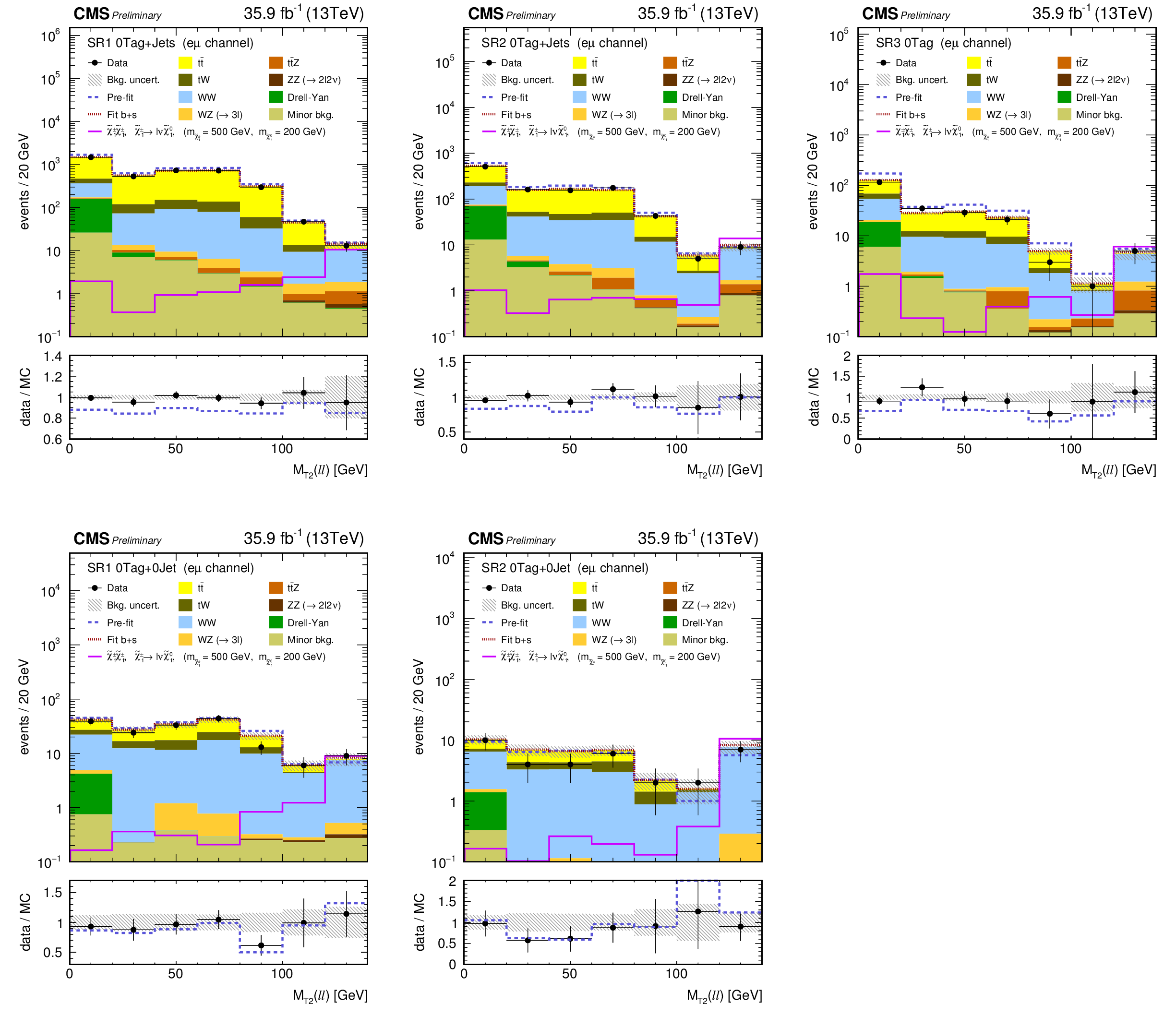
png pdf	Figure 3: Distributions of ${M_{\text {T2}}(\ell \ell)}$ after the fit to data in the chargino signal regions with 140 $< {{p_{\mathrm {T}}} ^\text {miss}} <$ 200 GeV (left plots), 200 $< {{p_{\mathrm {T}}} ^\text {miss}} <$ 300 GeV (middle) and ${{p_{\mathrm {T}}} ^\text {miss}} >$ 300 GeV (right), for DF events without b-tagged jets but at least one jet (upper plots) and no jets (lower plots). The upper plot for the signal region with ${{p_{\mathrm {T}}} ^\text {miss}} >$ 300 GeV shows all the events without b-tagged jets regardless of their jet multiplicity. Expected total SM contributions before the fit (dark blue dashed line) and after a background+signal fit (dark red dotted line) are also shown. The ratio data/MC is shown for the expected total SM contribution after the fit using the only background hypothesis (black dots) and before any fit (dark blue dashed line). The hatched band represents the total uncertainty after the fit.
png pdf	Figure 3-a: Distribution of ${M_{\text {T2}}(\ell \ell)}$ after the fit to data in the chargino signal regions with 140 $< {{p_{\mathrm {T}}} ^\text {miss}} <$ 200 GeV, for DF events without b-tagged jets but at least one jet. Expected total SM contributions before the fit (dark blue dashed line) and after a background+signal fit (dark red dotted line) are also shown. The ratio data/MC is shown for the expected total SM contribution after the fit using the only background hypothesis (black dots) and before any fit (dark blue dashed line). The hatched band represents the total uncertainty after the fit.
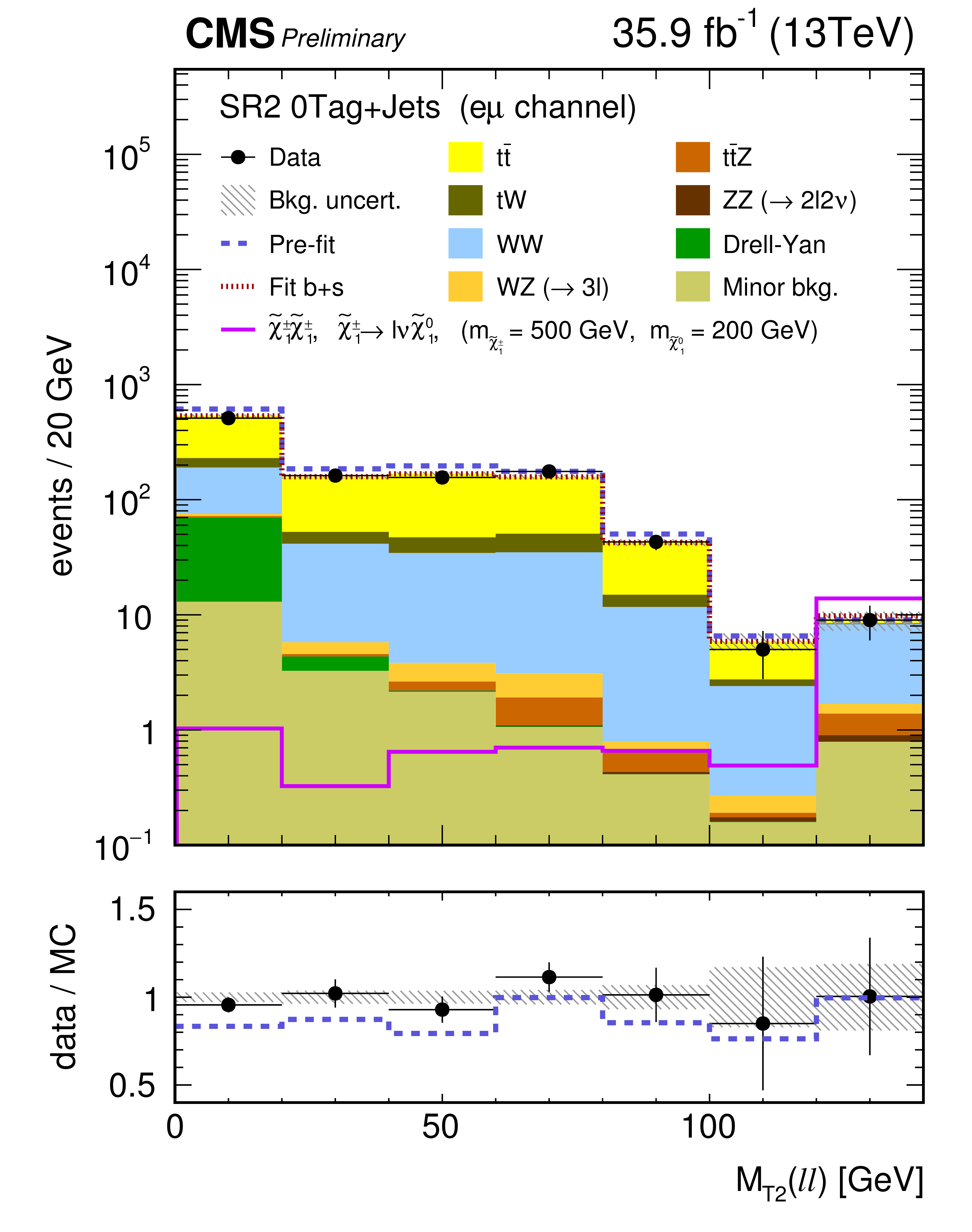
png pdf	Figure 3-b: Distribution of ${M_{\text {T2}}(\ell \ell)}$ after the fit to data in the chargino signal regions with 200 $< {{p_{\mathrm {T}}} ^\text {miss}} <$ 300 GeV, for DF events without b-tagged jets but at least one jet. Expected total SM contributions before the fit (dark blue dashed line) and after a background+signal fit (dark red dotted line) are also shown. The ratio data/MC is shown for the expected total SM contribution after the fit using the only background hypothesis (black dots) and before any fit (dark blue dashed line). The hatched band represents the total uncertainty after the fit.
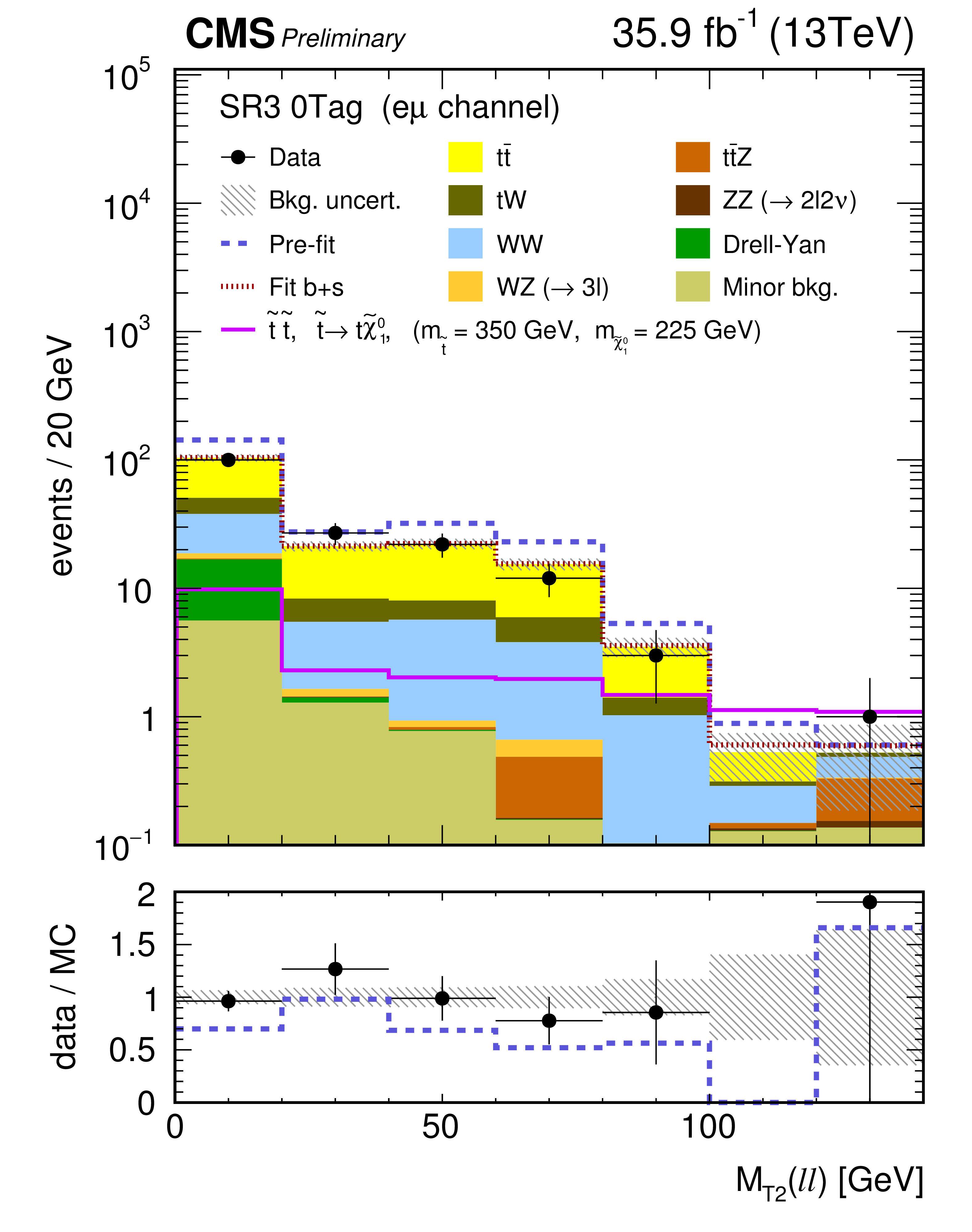
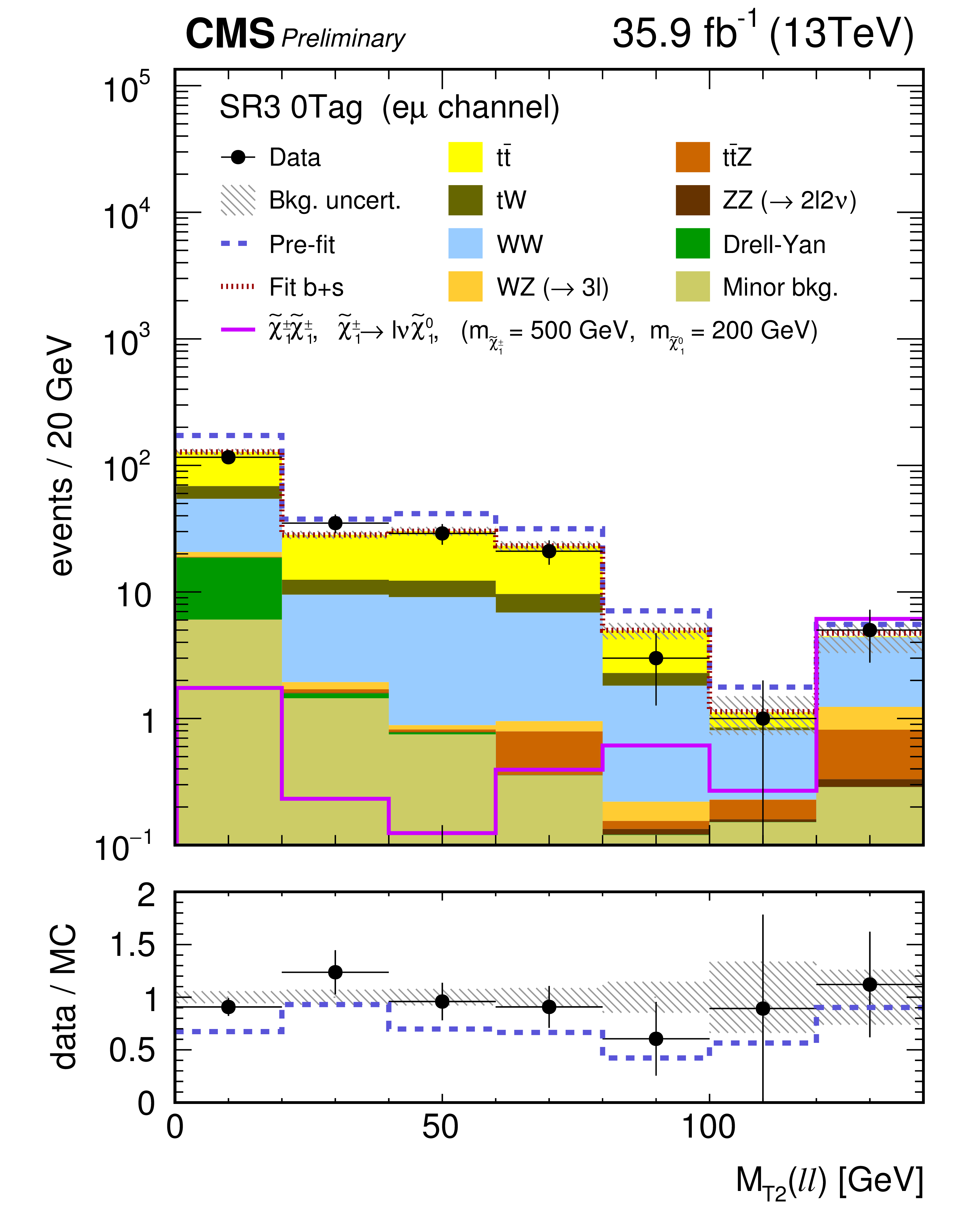
png pdf	Figure 3-c: Distribution of ${M_{\text {T2}}(\ell \ell)}$ after the fit to data in the chargino signal regions with ${{p_{\mathrm {T}}} ^\text {miss}} >$ 300 GeV, for DF events without b-tagged jets regardless of their jet multiplicity. Expected total SM contributions before the fit (dark blue dashed line) and after a background+signal fit (dark red dotted line) are also shown. The ratio data/MC is shown for the expected total SM contribution after the fit using the only background hypothesis (black dots) and before any fit (dark blue dashed line). The hatched band represents the total uncertainty after the fit.
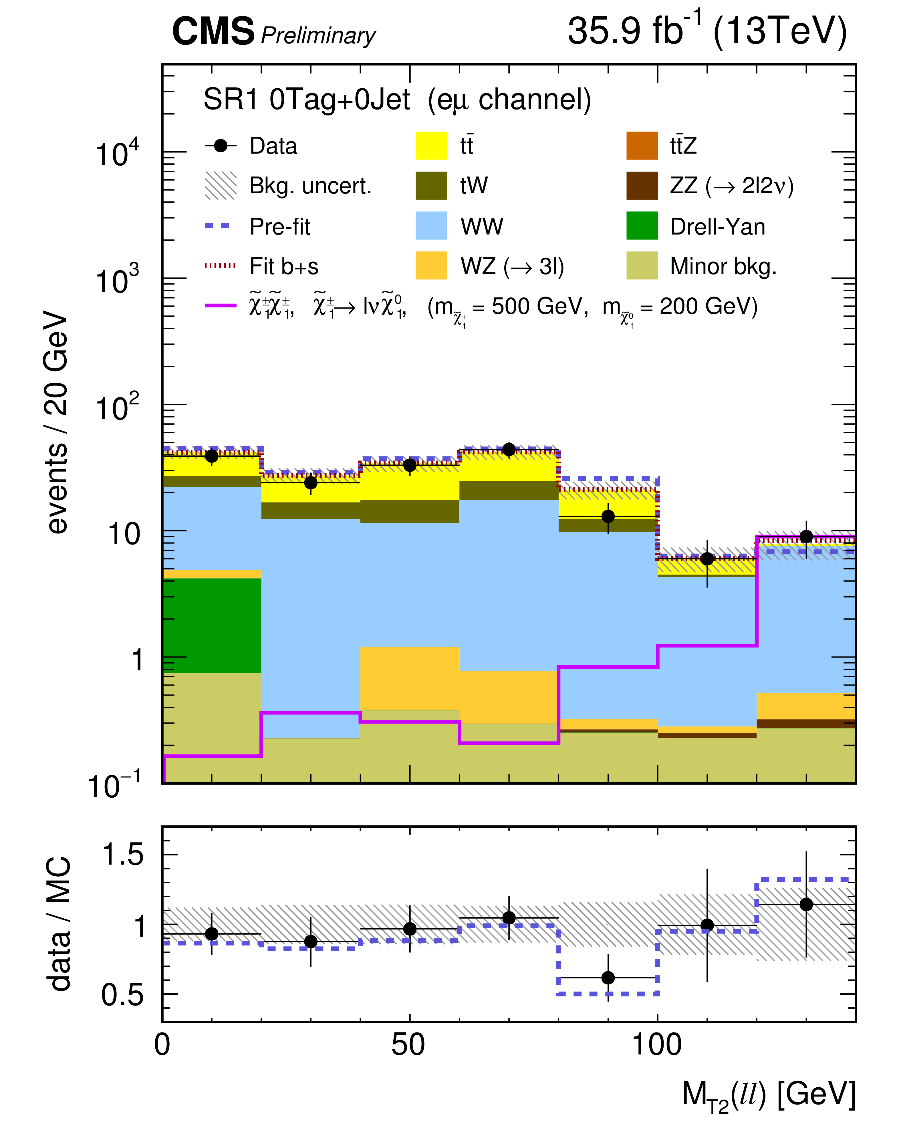
png pdf	Figure 3-d: Distribution of ${M_{\text {T2}}(\ell \ell)}$ after the fit to data in the chargino signal regions with 140 $< {{p_{\mathrm {T}}} ^\text {miss}} <$ 200 GeV, for DF events with no jet. Expected total SM contributions before the fit (dark blue dashed line) and after a background+signal fit (dark red dotted line) are also shown. The ratio data/MC is shown for the expected total SM contribution after the fit using the only background hypothesis (black dots) and before any fit (dark blue dashed line). The hatched band represents the total uncertainty after the fit.
png pdf	Figure 3-e: Distribution of ${M_{\text {T2}}(\ell \ell)}$ after the fit to data in the chargino signal regions with 200 $< {{p_{\mathrm {T}}} ^\text {miss}} <$ 300 GeV, for DF events with no jet. Expected total SM contributions before the fit (dark blue dashed line) and after a background+signal fit (dark red dotted line) are also shown. The ratio data/MC is shown for the expected total SM contribution after the fit using the only background hypothesis (black dots) and before any fit (dark blue dashed line). The hatched band represents the total uncertainty after the fit.
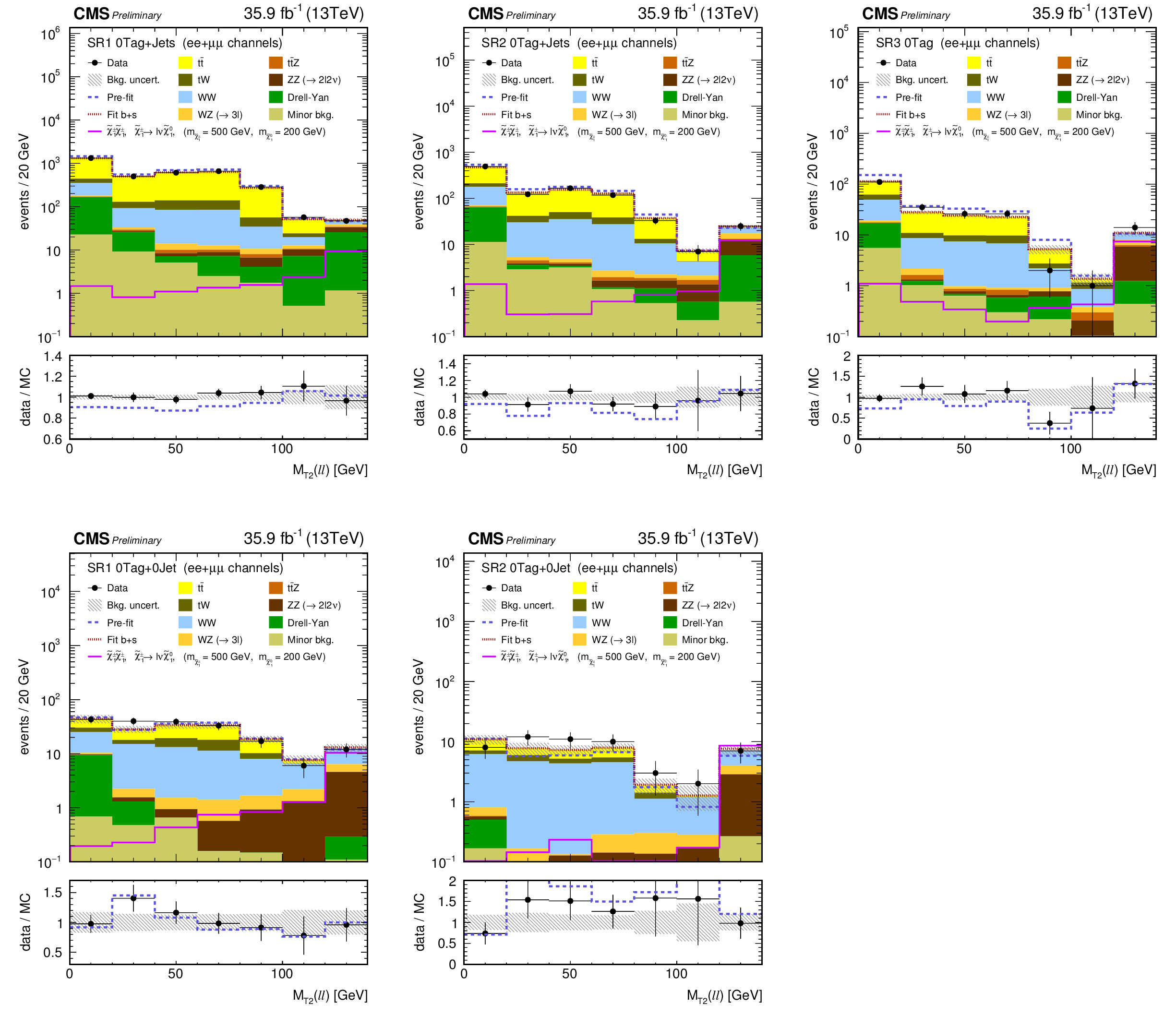
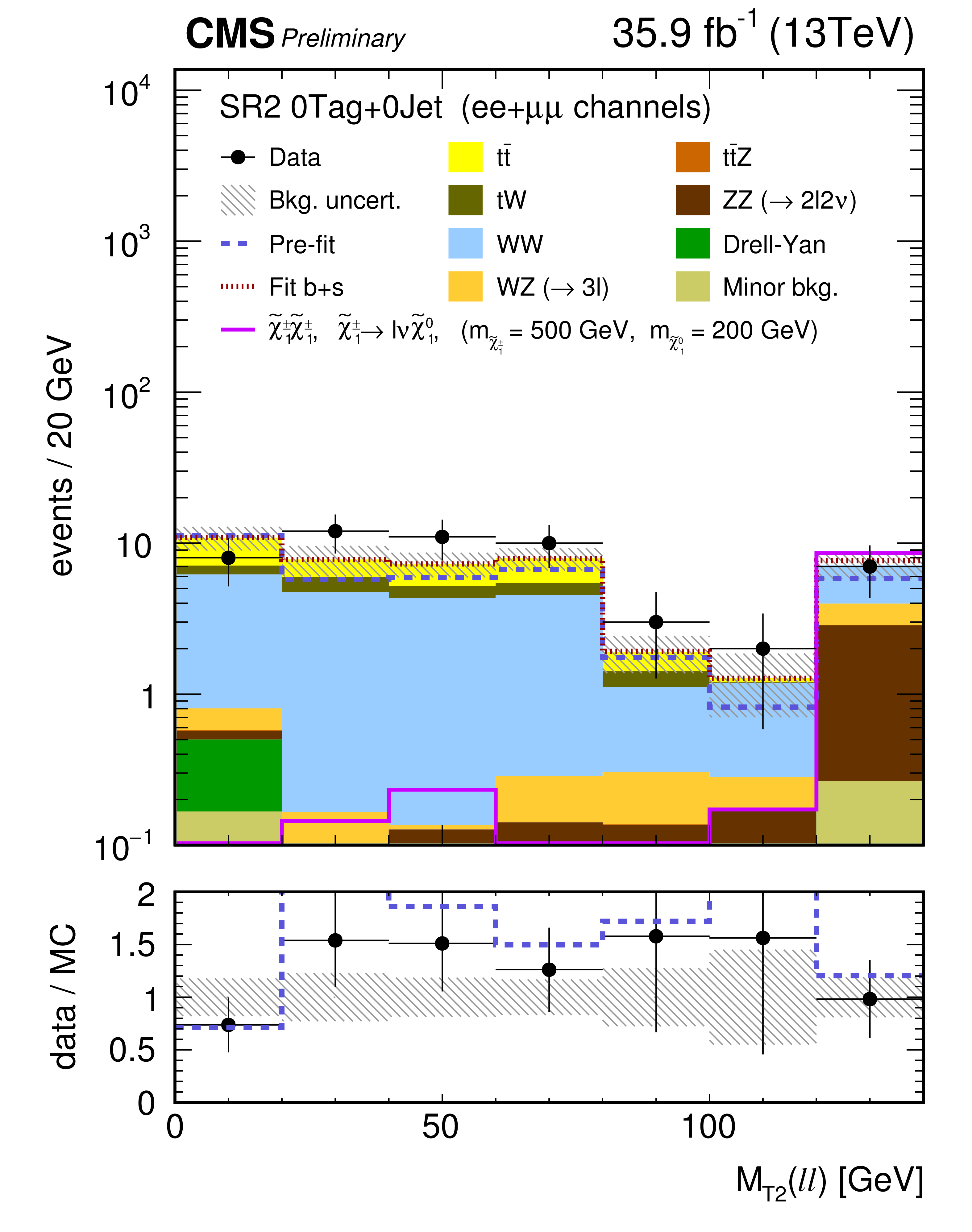
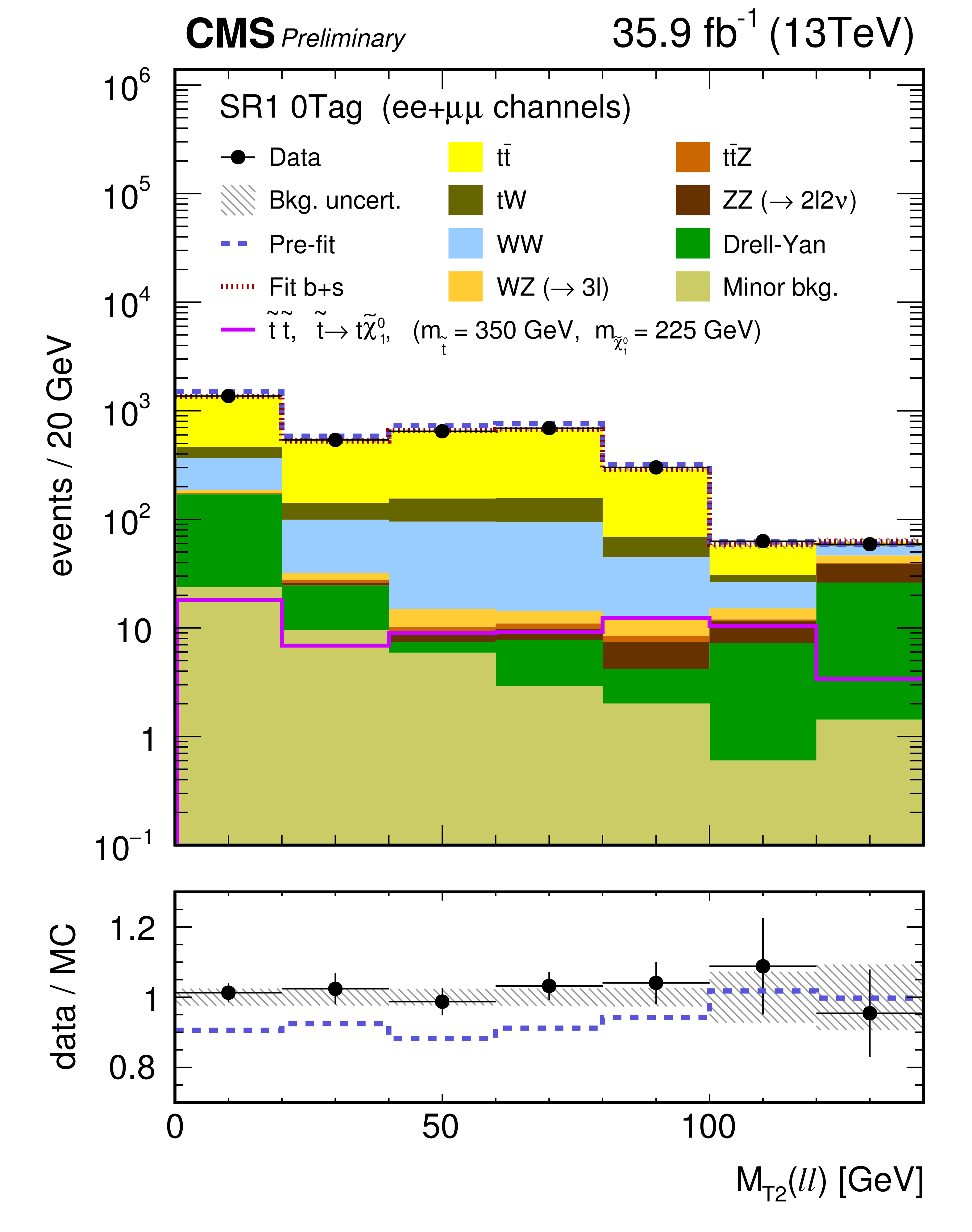
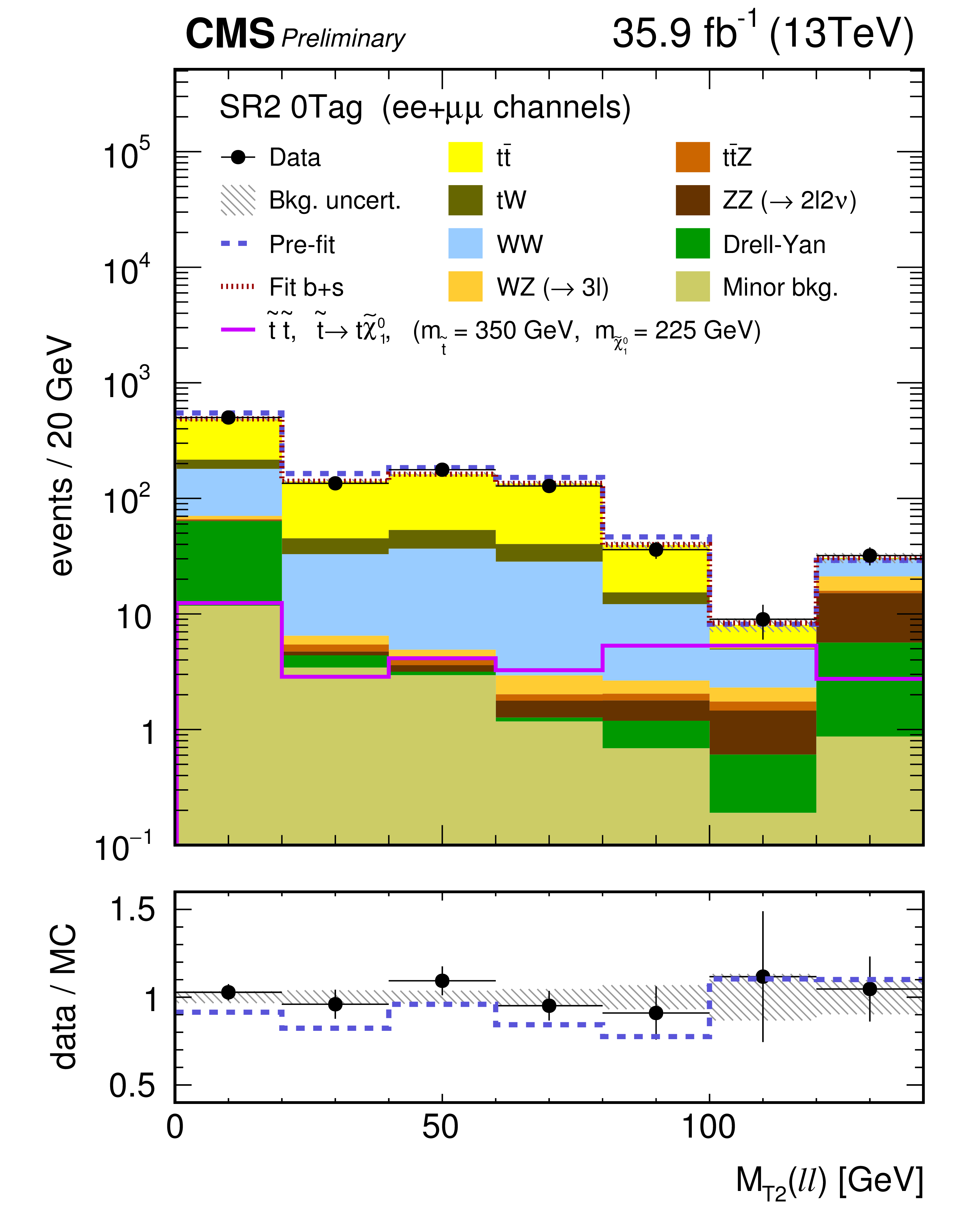
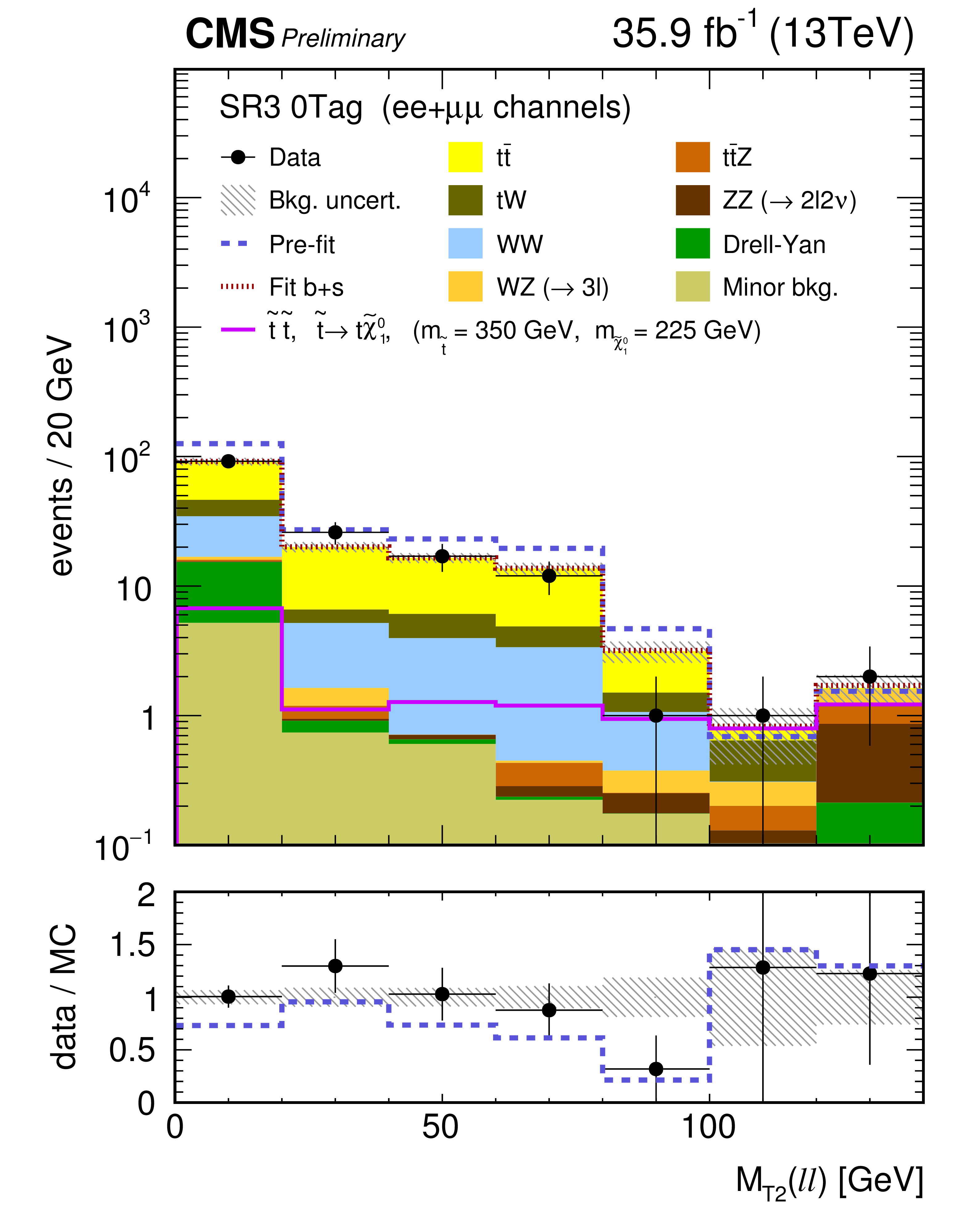
png pdf	Figure 4: Distributions of ${M_{\text {T2}}(\ell \ell)}$ after the fit to data in the chargino signal regions with 140 $< {{p_{\mathrm {T}}} ^\text {miss}} <$ 200 GeV (left plots), 200 $< {{p_{\mathrm {T}}} ^\text {miss}} <$ 300 GeV (middle) and ${{p_{\mathrm {T}}} ^\text {miss}} >$ 300 GeV (right), for SF events without b-tagged jets but at least one jet (upper plots) and no jets (lower plots). The upper plot for the signal region with ${{p_{\mathrm {T}}} ^\text {miss}} >$ 300 GeV shows all the events without b-tagged jets regardless of their jet multiplicity. Expected total SM contributions before the fit (dark blue dashed line) and after a background+signal fit (dark red dotted line) are also shown. The ratio data/MC is shown for the expected total SM contribution after the fit using the only background hypothesis (black dots) and before any fit (dark blue dashed line). The hatched band represents the total uncertainty after the fit.
png pdf	Figure 4-a: Distribution of ${M_{\text {T2}}(\ell \ell)}$ after the fit to data in the chargino signal regions with 140 $< {{p_{\mathrm {T}}} ^\text {miss}} <$ 200 GeV, for SF events without b-tagged jets but at least one jet. Expected total SM contributions before the fit (dark blue dashed line) and after a background+signal fit (dark red dotted line) are also shown. The ratio data/MC is shown for the expected total SM contribution after the fit using the only background hypothesis (black dots) and before any fit (dark blue dashed line). The hatched band represents the total uncertainty after the fit.
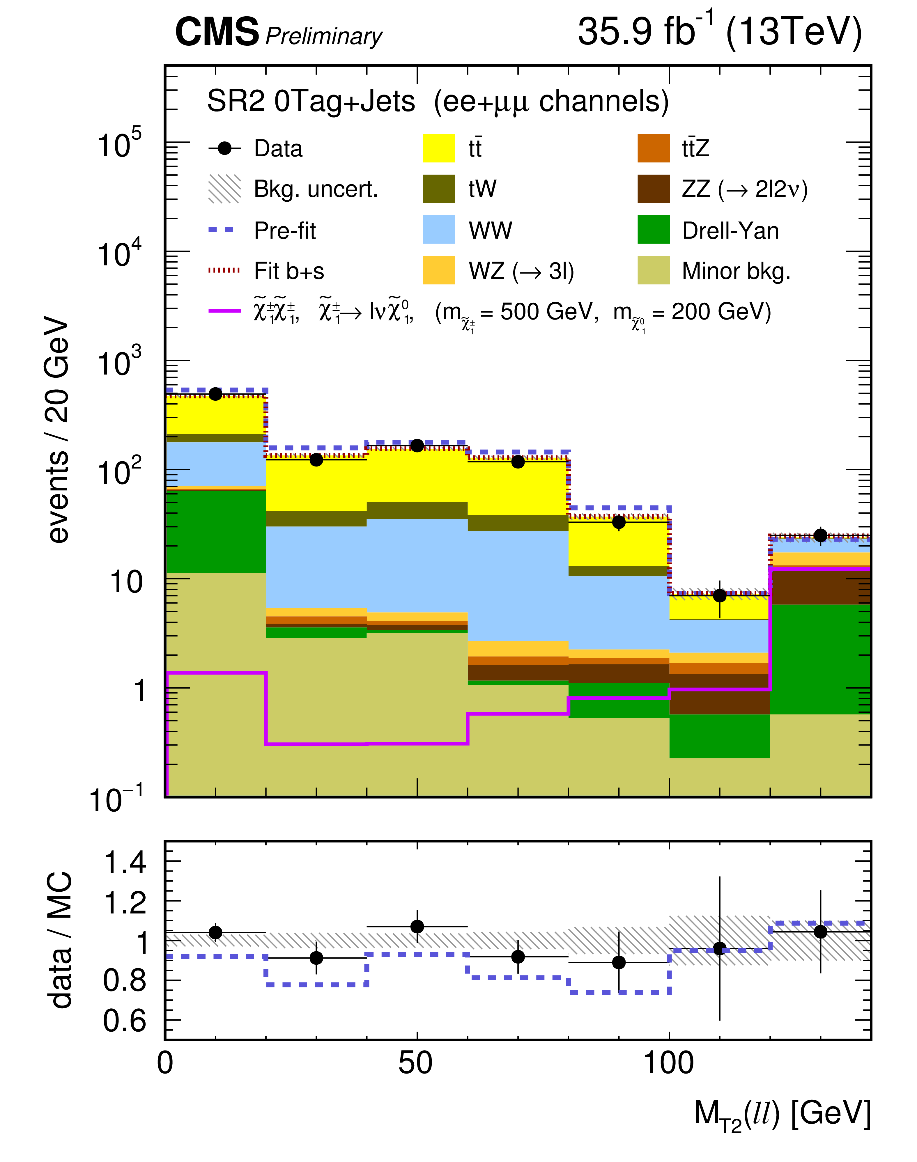
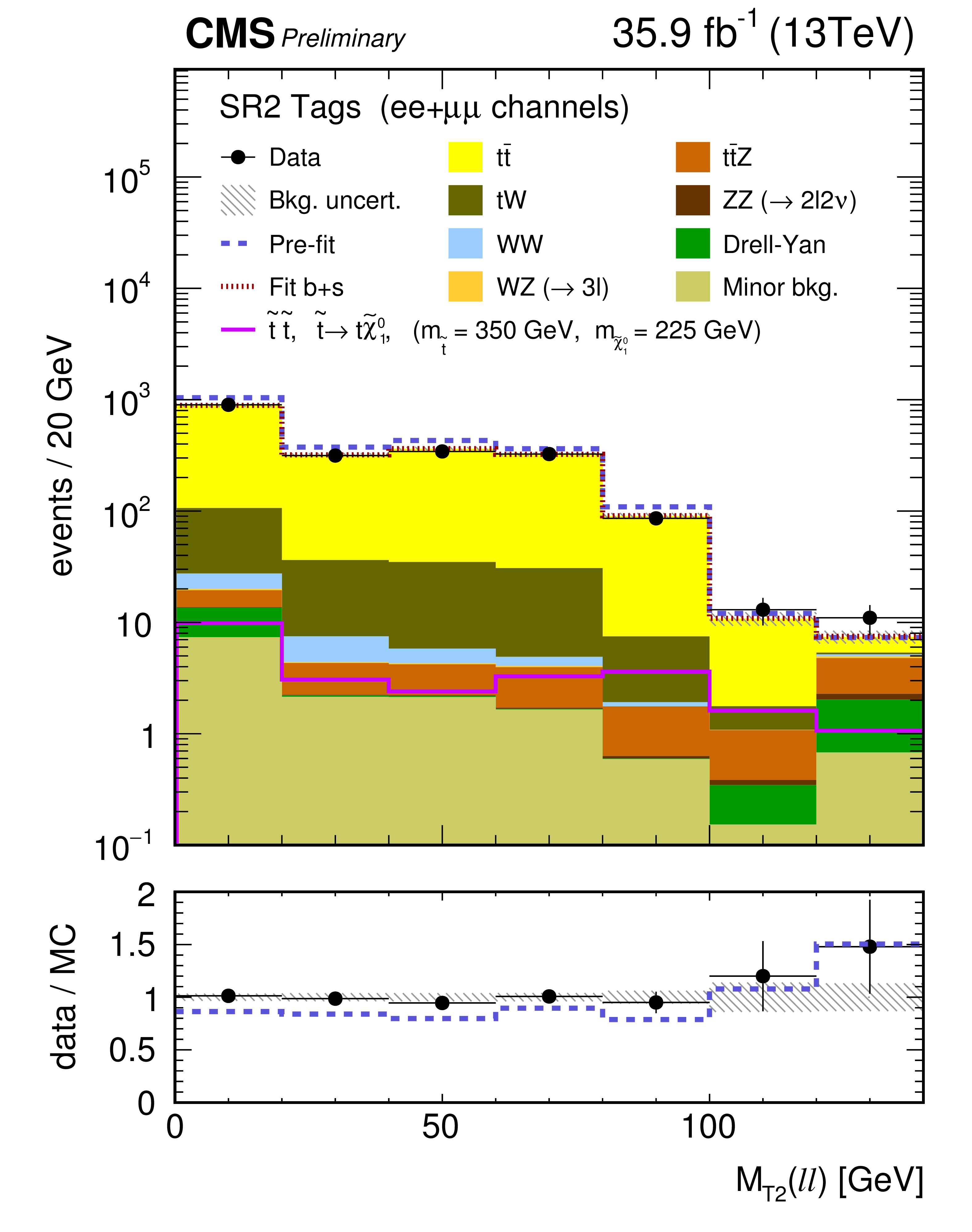
png pdf	Figure 4-b: Distribution of ${M_{\text {T2}}(\ell \ell)}$ after the fit to data in the chargino signal regions with 200 $< {{p_{\mathrm {T}}} ^\text {miss}} <$ 300 GeV, for SF events without b-tagged jets but at least one jet. Expected total SM contributions before the fit (dark blue dashed line) and after a background+signal fit (dark red dotted line) are also shown. The ratio data/MC is shown for the expected total SM contribution after the fit using the only background hypothesis (black dots) and before any fit (dark blue dashed line). The hatched band represents the total uncertainty after the fit.
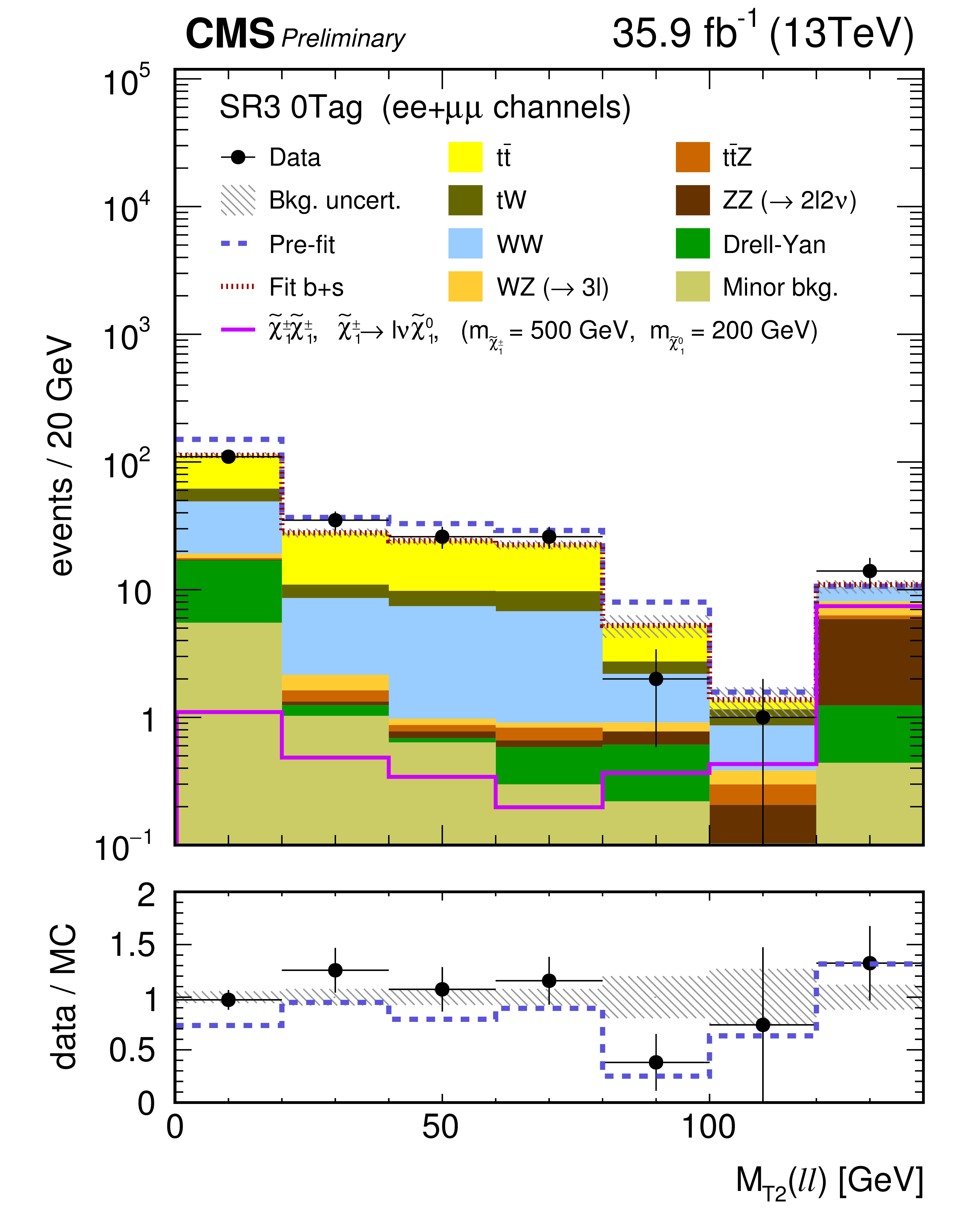
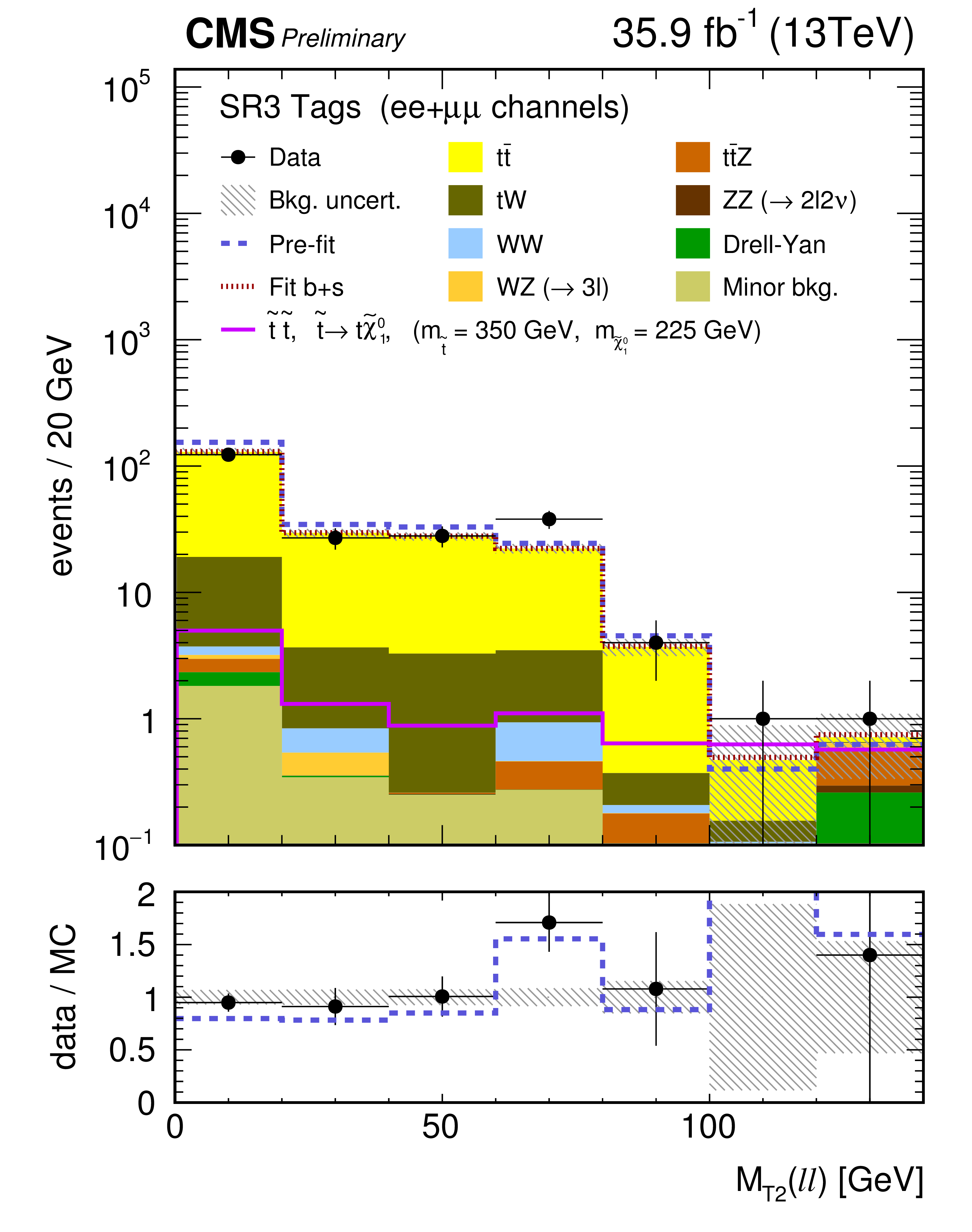
png pdf	Figure 4-c: Distribution of ${M_{\text {T2}}(\ell \ell)}$ after the fit to data in the chargino signal regions with ${{p_{\mathrm {T}}} ^\text {miss}} >$ 300 GeV (right), for SF events without b-tagged jets regardless of their jet multiplicity. Expected total SM contributions before the fit (dark blue dashed line) and after a background+signal fit (dark red dotted line) are also shown. The ratio data/MC is shown for the expected total SM contribution after the fit using the only background hypothesis (black dots) and before any fit (dark blue dashed line). The hatched band represents the total uncertainty after the fit.
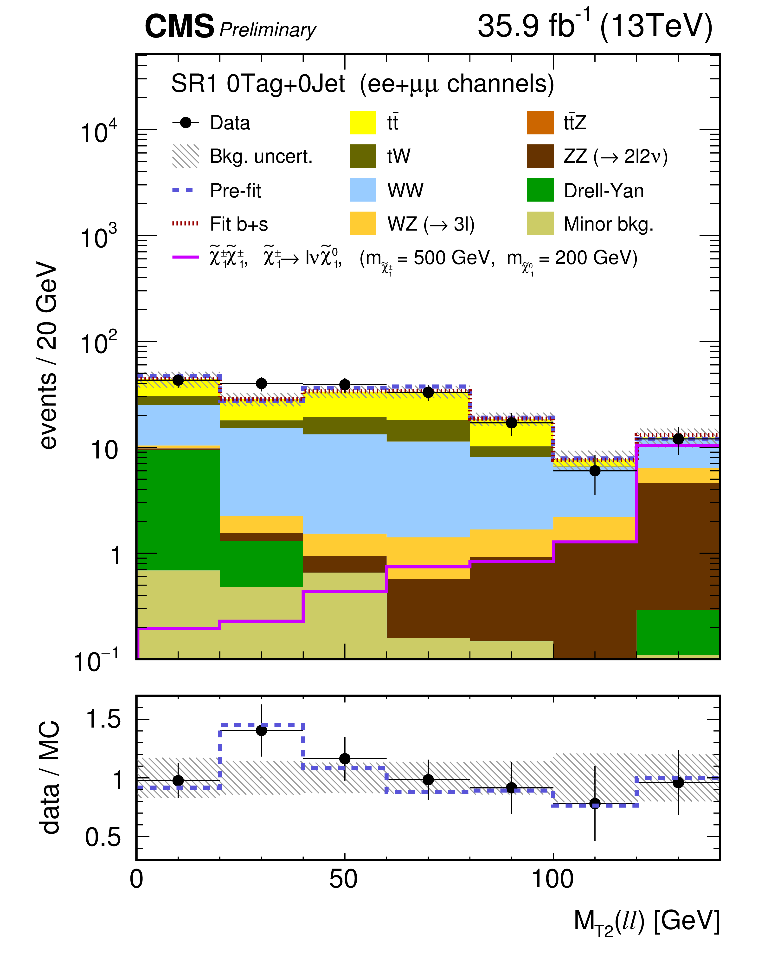
png pdf	Figure 4-d: Distribution of ${M_{\text {T2}}(\ell \ell)}$ after the fit to data in the chargino signal regions with 140 $< {{p_{\mathrm {T}}} ^\text {miss}} <$ 200 GeV, for SF events with no jets. Expected total SM contributions before the fit (dark blue dashed line) and after a background+signal fit (dark red dotted line) are also shown. The ratio data/MC is shown for the expected total SM contribution after the fit using the only background hypothesis (black dots) and before any fit (dark blue dashed line). The hatched band represents the total uncertainty after the fit.
png pdf	Figure 4-e: Distribution of ${M_{\text {T2}}(\ell \ell)}$ after the fit to data in the chargino signal regions with 200 $< {{p_{\mathrm {T}}} ^\text {miss}} <$ 300 GeV, for SF events with no jets. Expected total SM contributions before the fit (dark blue dashed line) and after a background+signal fit (dark red dotted line) are also shown. The ratio data/MC is shown for the expected total SM contribution after the fit using the only background hypothesis (black dots) and before any fit (dark blue dashed line). The hatched band represents the total uncertainty after the fit.
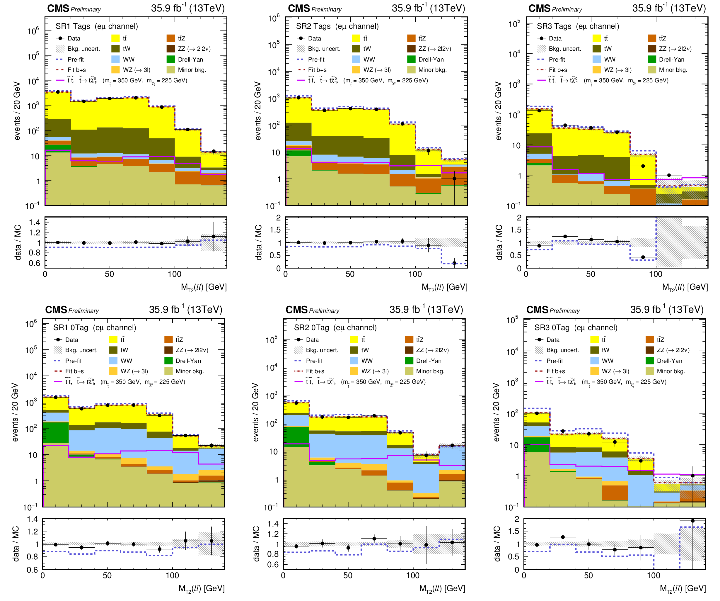
png pdf	Figure 5: Distributions of ${M_{\text {T2}}(\ell \ell)}$ after the fit to data in the top squark signal regions with 140 $< {{p_{\mathrm {T}}} ^\text {miss}} <$ 200 GeV (left plots), 200 $< {{p_{\mathrm {T}}} ^\text {miss}} <$ 300 GeV (middle), or ${{p_{\mathrm {T}}} ^\text {miss}} >$ 300 GeV (right), for DF events with b-tagged jets (upper plots) and without b-tagged jets (lower plots). Expected total SM contributions before the fit (dark blue dashed line) and after a background+signal fit (dark red dotted line) are also shown. The ratio data/MC is shown for the expected total SM contribution after the fit using the only background hypothesis (black dots) and before any fit (dark blue dashed line). The hatched band represents the total uncertainty after the fit.
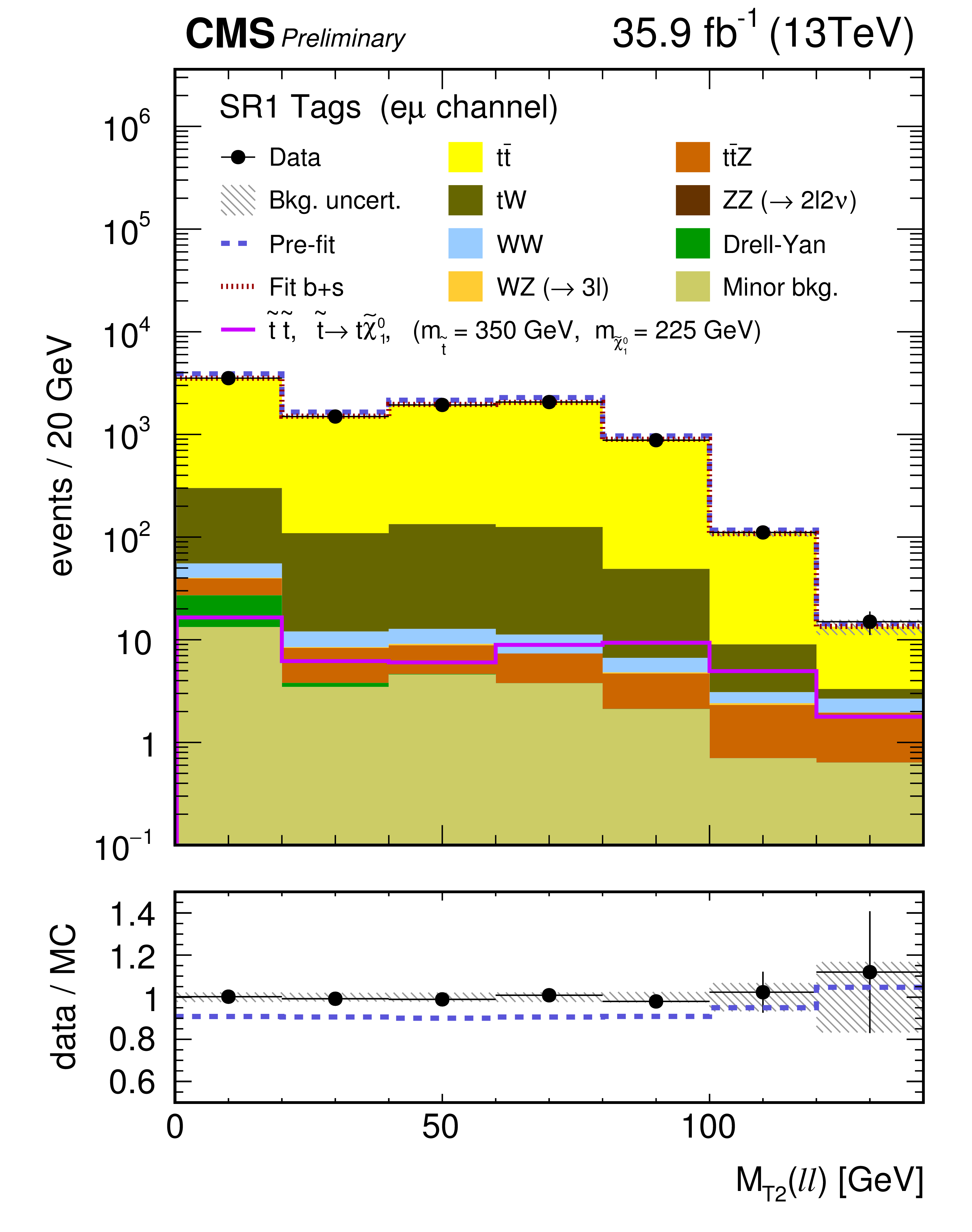
png pdf	Figure 5-a: Distribution of ${M_{\text {T2}}(\ell \ell)}$ after the fit to data in the top squark signal regions with 140 $< {{p_{\mathrm {T}}} ^\text {miss}} <$ 200 GeV, for DF events with b-tagged jets. Expected total SM contributions before the fit (dark blue dashed line) and after a background+signal fit (dark red dotted line) are also shown. The ratio data/MC is shown for the expected total SM contribution after the fit using the only background hypothesis (black dots) and before any fit (dark blue dashed line). The hatched band represents the total uncertainty after the fit.
png pdf	Figure 5-b: Distribution of ${M_{\text {T2}}(\ell \ell)}$ after the fit to data in the top squark signal regions with 200 $< {{p_{\mathrm {T}}} ^\text {miss}} <$ 300 GeV, for DF events with b-tagged jets. Expected total SM contributions before the fit (dark blue dashed line) and after a background+signal fit (dark red dotted line) are also shown. The ratio data/MC is shown for the expected total SM contribution after the fit using the only background hypothesis (black dots) and before any fit (dark blue dashed line). The hatched band represents the total uncertainty after the fit.
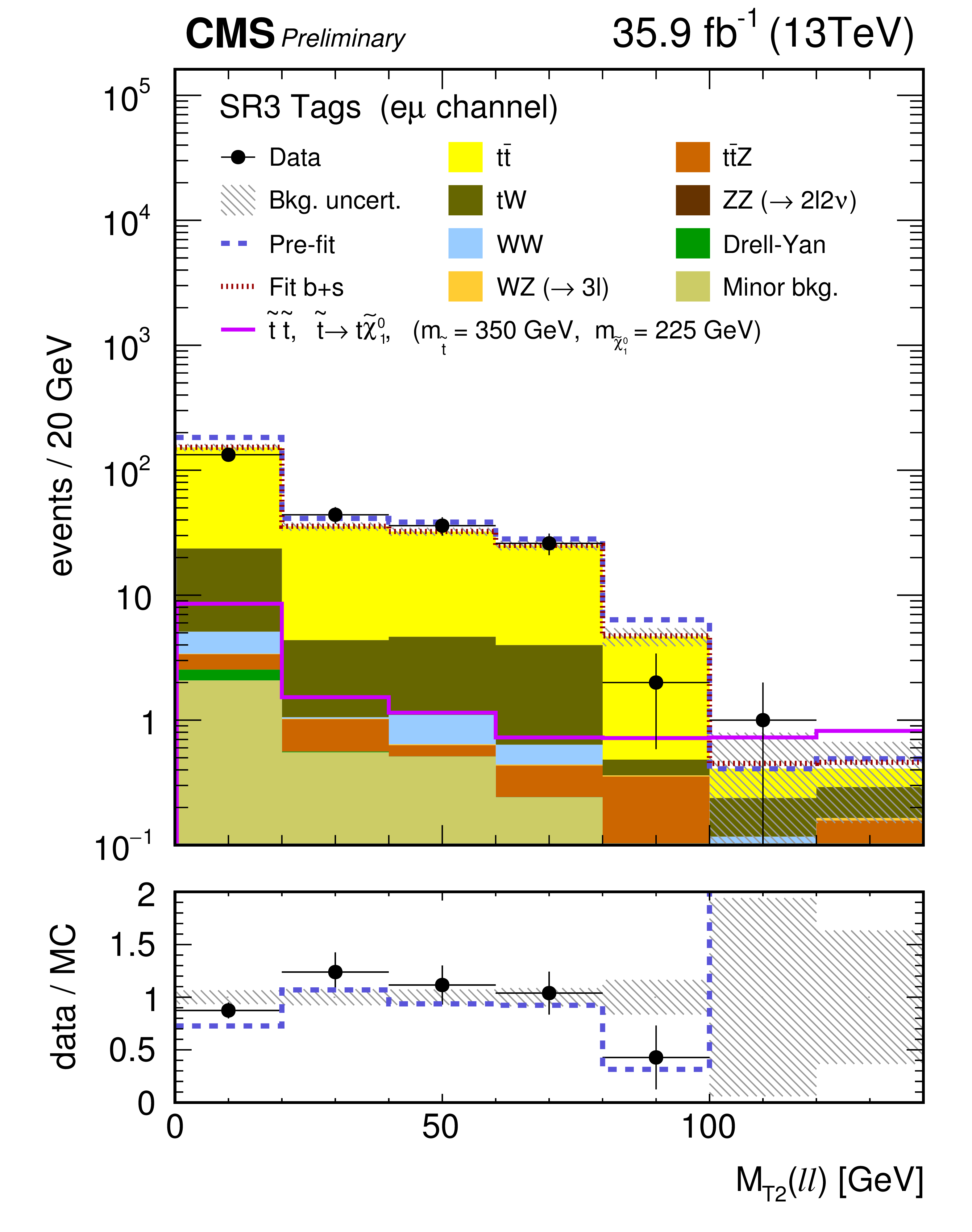
png pdf	Figure 5-c: Distribution of ${M_{\text {T2}}(\ell \ell)}$ after the fit to data in the top squark signal regions with ${{p_{\mathrm {T}}} ^\text {miss}} >$ 300 GeV, for DF events with b-tagged jets. Expected total SM contributions before the fit (dark blue dashed line) and after a background+signal fit (dark red dotted line) are also shown. The ratio data/MC is shown for the expected total SM contribution after the fit using the only background hypothesis (black dots) and before any fit (dark blue dashed line). The hatched band represents the total uncertainty after the fit.
png pdf	Figure 5-d: Distribution of ${M_{\text {T2}}(\ell \ell)}$ after the fit to data in the top squark signal regions with 140 $< {{p_{\mathrm {T}}} ^\text {miss}} <$ 200 GeV, for DF events without b-tagged jets. Expected total SM contributions before the fit (dark blue dashed line) and after a background+signal fit (dark red dotted line) are also shown. The ratio data/MC is shown for the expected total SM contribution after the fit using the only background hypothesis (black dots) and before any fit (dark blue dashed line). The hatched band represents the total uncertainty after the fit.
png pdf	Figure 5-e: Distribution of ${M_{\text {T2}}(\ell \ell)}$ after the fit to data in the top squark signal regions with 200 $< {{p_{\mathrm {T}}} ^\text {miss}} <$ 300 GeV, for DF events without b-tagged jets. Expected total SM contributions before the fit (dark blue dashed line) and after a background+signal fit (dark red dotted line) are also shown. The ratio data/MC is shown for the expected total SM contribution after the fit using the only background hypothesis (black dots) and before any fit (dark blue dashed line). The hatched band represents the total uncertainty after the fit.
png pdf	Figure 5-f: Distribution of ${M_{\text {T2}}(\ell \ell)}$ after the fit to data in the top squark signal regions with ${{p_{\mathrm {T}}} ^\text {miss}} >$ 300 GeV, for DF events without b-tagged jets. Expected total SM contributions before the fit (dark blue dashed line) and after a background+signal fit (dark red dotted line) are also shown. The ratio data/MC is shown for the expected total SM contribution after the fit using the only background hypothesis (black dots) and before any fit (dark blue dashed line). The hatched band represents the total uncertainty after the fit.
png pdf	Figure 6: Distributions of ${M_{\text {T2}}(\ell \ell)}$ after the fit to data in the top squark signal regions with 140 $< {{p_{\mathrm {T}}} ^\text {miss}} <$ 200 GeV (left plots), 200 $< {{p_{\mathrm {T}}} ^\text {miss}} <$ 300 GeV (middle), or ${{p_{\mathrm {T}}} ^\text {miss}} >$ 300 GeV (right), for SF events with b-tagged jets (upper plots) and without b-tagged jets (lower plots). Expected total SM contributions before the fit (dark blue dashed line) and after a background+signal fit (dark red dotted line) are also shown. The ratio data/MC is shown for the expected total SM contribution after the fit using the only background hypothesis (black dots) and before any fit (dark blue dashed line). The hatched band represents the total uncertainty after the fit.
png pdf	Figure 6-a: Distribution of ${M_{\text {T2}}(\ell \ell)}$ after the fit to data in the top squark signal regions with 140 $< {{p_{\mathrm {T}}} ^\text {miss}} <$ 200 GeV, for SF events with b-tagged jets. Expected total SM contributions before the fit (dark blue dashed line) and after a background+signal fit (dark red dotted line) are also shown. The ratio data/MC is shown for the expected total SM contribution after the fit using the only background hypothesis (black dots) and before any fit (dark blue dashed line). The hatched band represents the total uncertainty after the fit.
png pdf	Figure 6-b: Distribution of ${M_{\text {T2}}(\ell \ell)}$ after the fit to data in the top squark signal regions with 200 $< {{p_{\mathrm {T}}} ^\text {miss}} <$ 300 GeV, for SF events with b-tagged jets. Expected total SM contributions before the fit (dark blue dashed line) and after a background+signal fit (dark red dotted line) are also shown. The ratio data/MC is shown for the expected total SM contribution after the fit using the only background hypothesis (black dots) and before any fit (dark blue dashed line). The hatched band represents the total uncertainty after the fit.
png pdf	Figure 6-c: Distribution of ${M_{\text {T2}}(\ell \ell)}$ after the fit to data in the top squark signal regions with ${{p_{\mathrm {T}}} ^\text {miss}} >$ 300 GeV, for SF events with b-tagged jets. Expected total SM contributions before the fit (dark blue dashed line) and after a background+signal fit (dark red dotted line) are also shown. The ratio data/MC is shown for the expected total SM contribution after the fit using the only background hypothesis (black dots) and before any fit (dark blue dashed line). The hatched band represents the total uncertainty after the fit.
png pdf	Figure 6-d: Distribution of ${M_{\text {T2}}(\ell \ell)}$ after the fit to data in the top squark signal regions with 140 $< {{p_{\mathrm {T}}} ^\text {miss}} <$ 200 GeV, for SF events without b-tagged jets. Expected total SM contributions before the fit (dark blue dashed line) and after a background+signal fit (dark red dotted line) are also shown. The ratio data/MC is shown for the expected total SM contribution after the fit using the only background hypothesis (black dots) and before any fit (dark blue dashed line). The hatched band represents the total uncertainty after the fit.
png pdf	Figure 6-e: Distribution of ${M_{\text {T2}}(\ell \ell)}$ after the fit to data in the top squark signal regions with 200 $< {{p_{\mathrm {T}}} ^\text {miss}} <$ 300 GeV, for SF events without b-tagged jets. Expected total SM contributions before the fit (dark blue dashed line) and after a background+signal fit (dark red dotted line) are also shown. The ratio data/MC is shown for the expected total SM contribution after the fit using the only background hypothesis (black dots) and before any fit (dark blue dashed line). The hatched band represents the total uncertainty after the fit.
png pdf	Figure 6-f: Distribution of ${M_{\text {T2}}(\ell \ell)}$ after the fit to data in the top squark signal regions with ${{p_{\mathrm {T}}} ^\text {miss}} >$ 300 GeV, for SF events without b-tagged jets. Expected total SM contributions before the fit (dark blue dashed line) and after a background+signal fit (dark red dotted line) are also shown. The ratio data/MC is shown for the expected total SM contribution after the fit using the only background hypothesis (black dots) and before any fit (dark blue dashed line). The hatched band represents the total uncertainty after the fit.
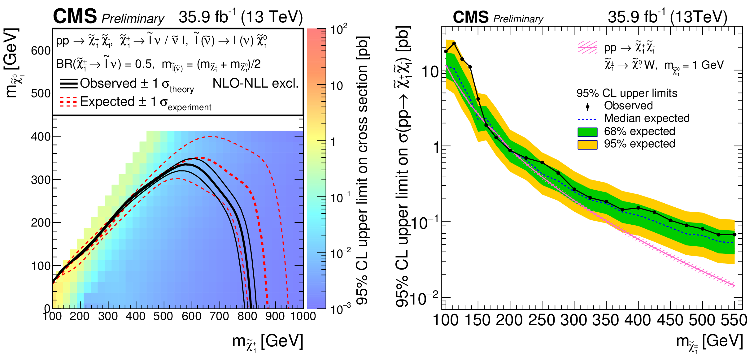
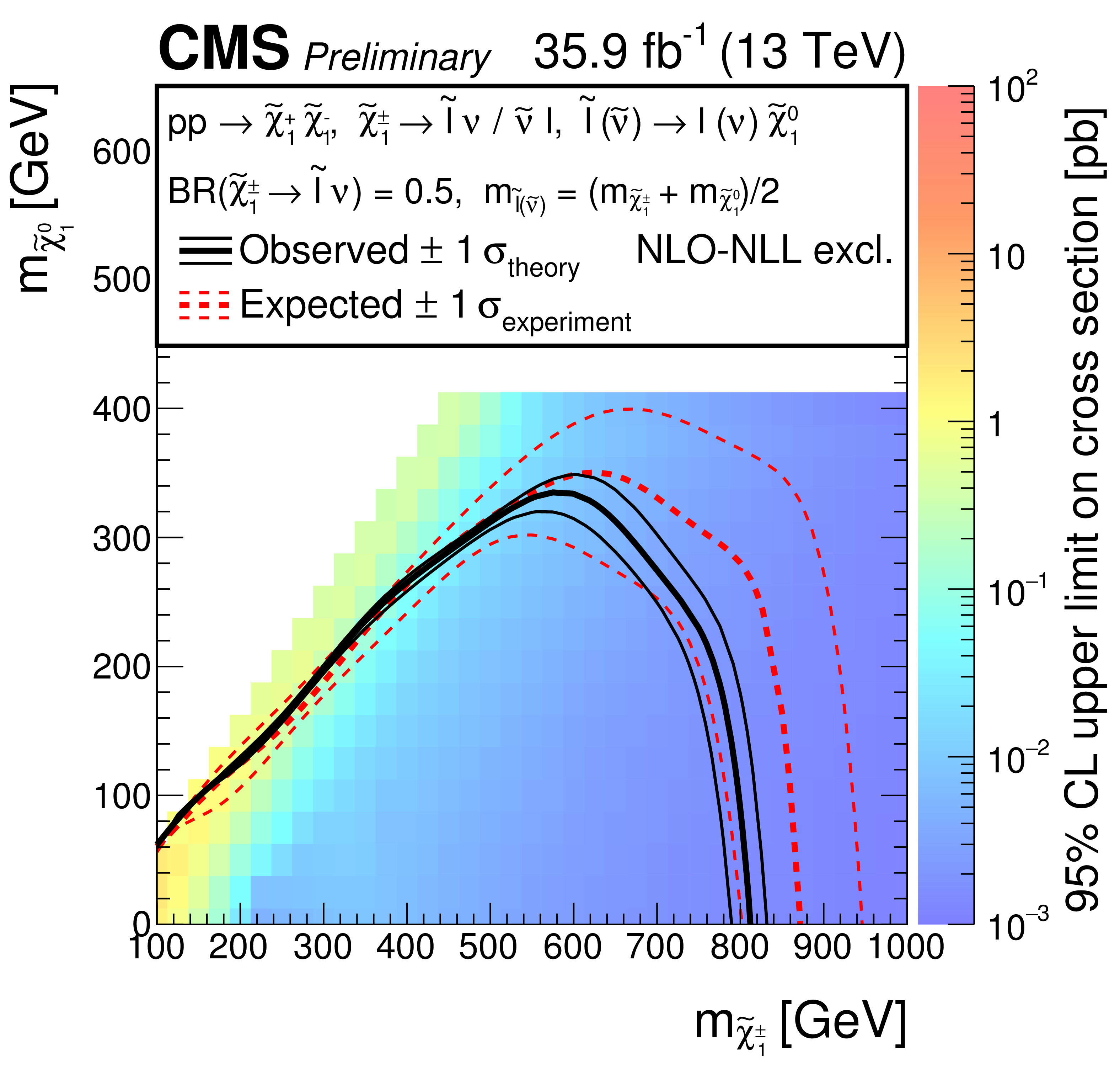
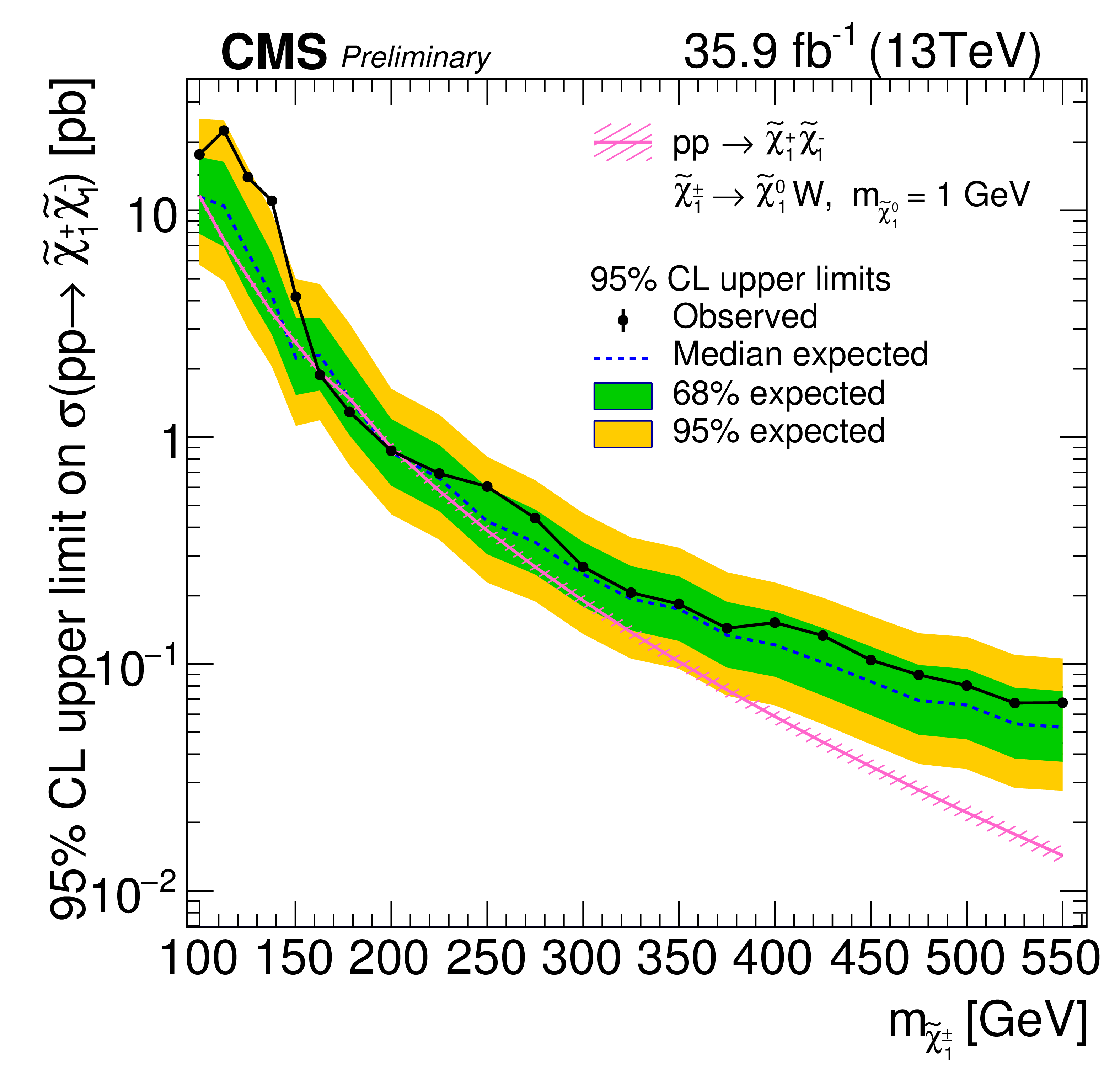
png pdf	Figure 7: Left: upper limits at 95% CL on the chargino pair production cross section as a function of the chargino and neutralino masses, when the chargino undergoes a cascade decay $\tilde{ \chi }^{\pm}_1 \rightarrow \tilde{ \ell }\nu (\ell \tilde{ \nu })\rightarrow \ell \nu \tilde{ \chi }^{0}_1$ . The thick dashed red line shows the expected exclusion region in the plane ( $m_{\tilde{ \chi }^{\pm}_1}, m_{\tilde{ \chi }^{0}_1}$ ). The thin dashed red lines show the variation of the exclusion regions due to the experimental uncertainties. The thick black line shows the observed exclusion region, while the thin black lines show the variation of the exclusion regions due to the theoretical uncertainties on the production cross section. Right: observed and expected upper limits at 95% CL as a function of the chargino mass for a neutralino mass of 1 GeV, assuming chargino decays into a neutralino and a W boson ( $\tilde{ \chi }^{\pm}_1 \rightarrow {\mathrm {W}} \tilde{ \chi }^{0}_1$ ).
png pdf	Figure 7-a: Upper limits at 95% CL on the chargino pair production cross section as a function of the chargino and neutralino masses, when the chargino undergoes a cascade decay $\tilde{ \chi }^{\pm}_1 \rightarrow \tilde{ \ell }\nu (\ell \tilde{ \nu })\rightarrow \ell \nu \tilde{ \chi }^{0}_1$ . The thick dashed red line shows the expected exclusion region in the plane ( $m_{\tilde{ \chi }^{\pm}_1}, m_{\tilde{ \chi }^{0}_1}$ ). The thin dashed red lines show the variation of the exclusion regions due to the experimental uncertainties. The thick black line shows the observed exclusion region, while the thin black lines show the variation of the exclusion regions due to the theoretical uncertainties on the production cross section.
png pdf	Figure 7-b: Observed and expected upper limits at 95% CL as a function of the chargino mass for a neutralino mass of 1 GeV, assuming chargino decays into a neutralino and a W boson ( $\tilde{ \chi }^{\pm}_1 \rightarrow {\mathrm {W}} \tilde{ \chi }^{0}_1$ ).
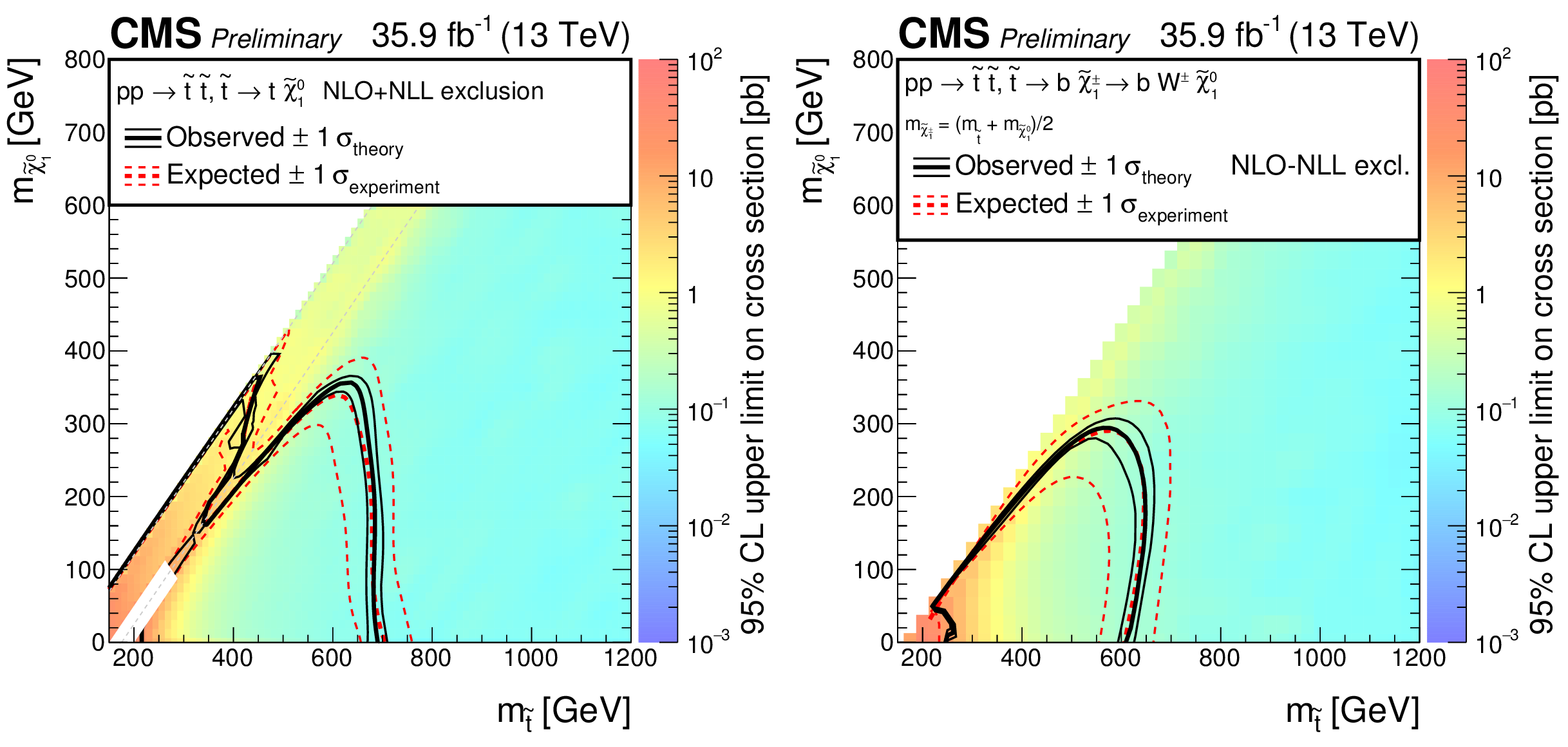
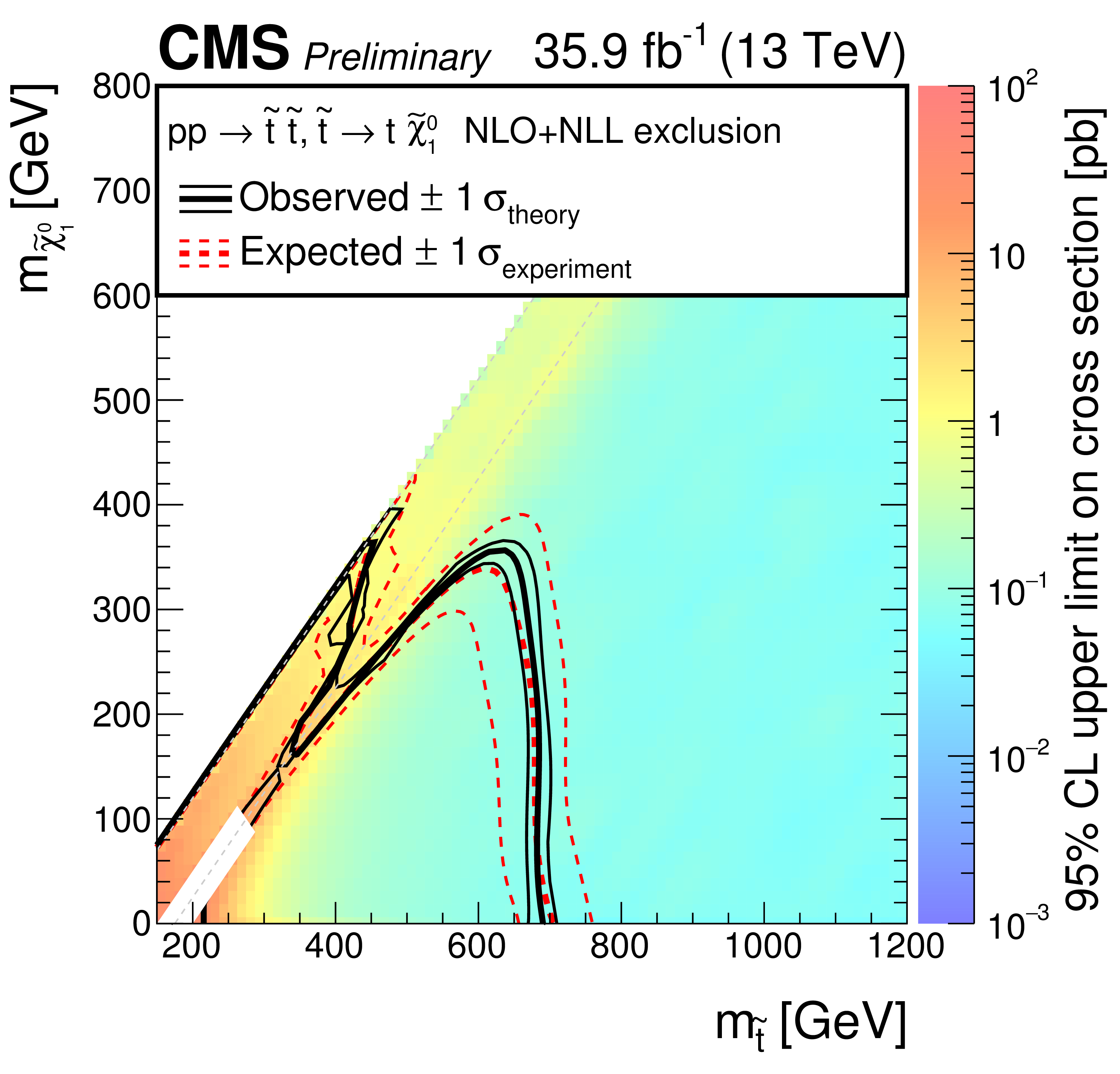
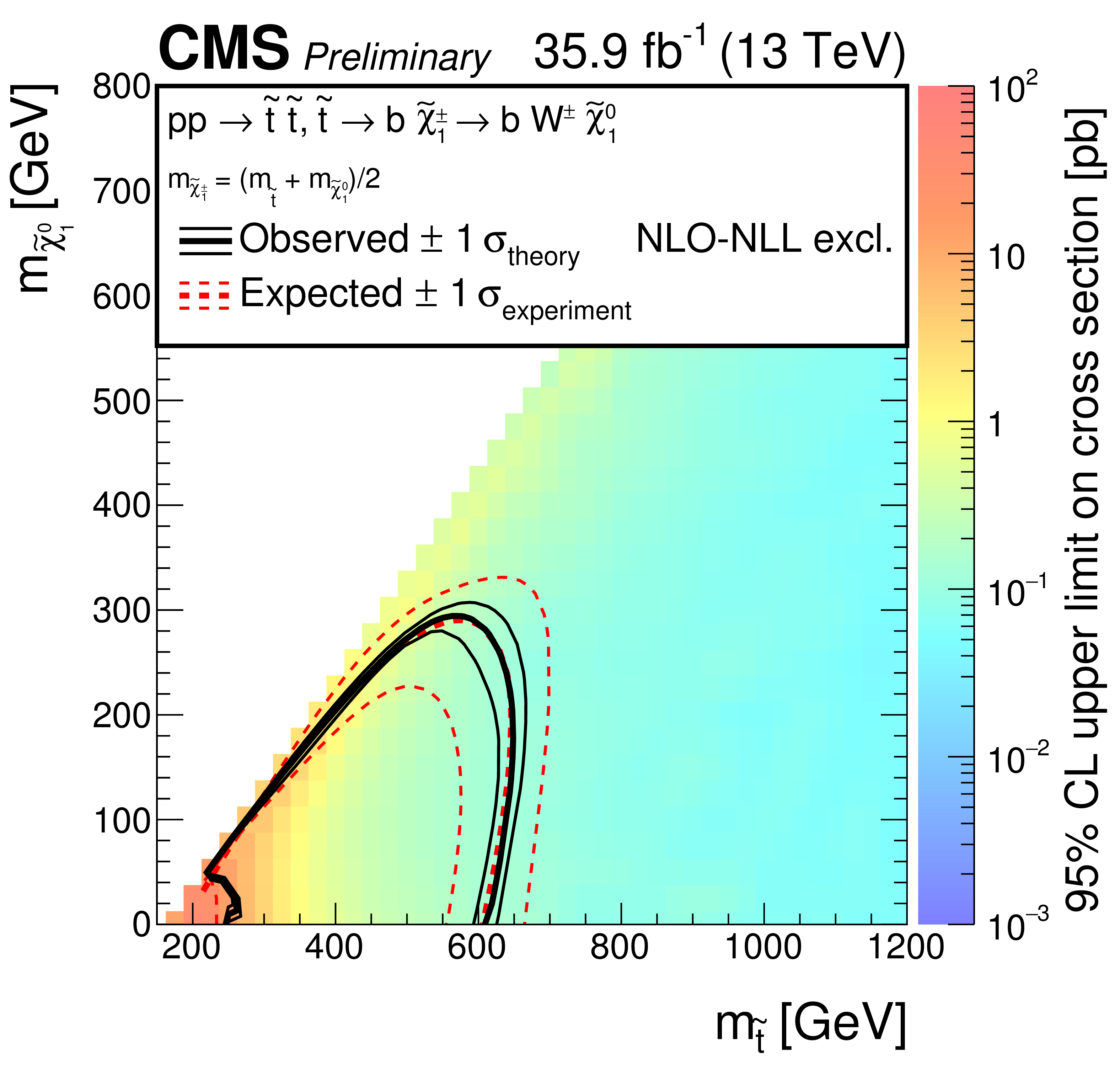
png pdf	Figure 8: Upper limits at 95% CL on the top squark production cross section as a function of the stop and neutralino masses. The plot on the left shows the results when top squark decays into a top quark and a neutralino are assumed. The plot on the right gives the limits for top squarks decaying into a bottom quark and a chargino, with the latter successively decaying into a W boson and a neutralino. The mass of the chargino is assumed to be equal to the average of the top squark and neutralino masses. The thick dashed red line shows the expected exclusion region in the plane ( $m_{\tilde{ \mathrm{t} }}$ , $m_{\tilde{ \chi }^{0}_1}$ ). The thin dashed red lines show the variation of the exclusion regions due to the experimental uncertainties. The thick black line shows the observed exclusion region, while the thin black lines show the variation of the exclusion regions due to the theoretical uncertainties on the production cross section.
png pdf	Figure 8-a: Upper limits at 95% CL on the top squark production cross section as a function of the stop and neutralino masses. The plot shows the results when top squark decays into a top quark and a neutralino are assumed. The thick dashed red line shows the expected exclusion region in the plane ( $m_{\tilde{ \mathrm{t} }}$ , $m_{\tilde{ \chi }^{0}_1}$ ). The thin dashed red lines show the variation of the exclusion regions due to the experimental uncertainties. The thick black line shows the observed exclusion region, while the thin black lines show the variation of the exclusion regions due to the theoretical uncertainties on the production cross section.
png pdf	Figure 8-b: Upper limits at 95% CL on the top squark production cross section as a function of the stop and neutralino masses. The plot gives the limits for top squarks decaying into a bottom quark and a chargino, with the latter successively decaying into a W boson and a neutralino. The mass of the chargino is assumed to be equal to the average of the top squark and neutralino masses. The thick dashed red line shows the expected exclusion region in the plane ( $m_{\tilde{ \mathrm{t} }}$ , $m_{\tilde{ \chi }^{0}_1}$ ). The thin dashed red lines show the variation of the exclusion regions due to the experimental uncertainties. The thick black line shows the observed exclusion region, while the thin black lines show the variation of the exclusion regions due to the theoretical uncertainties on the production cross section.

Tables
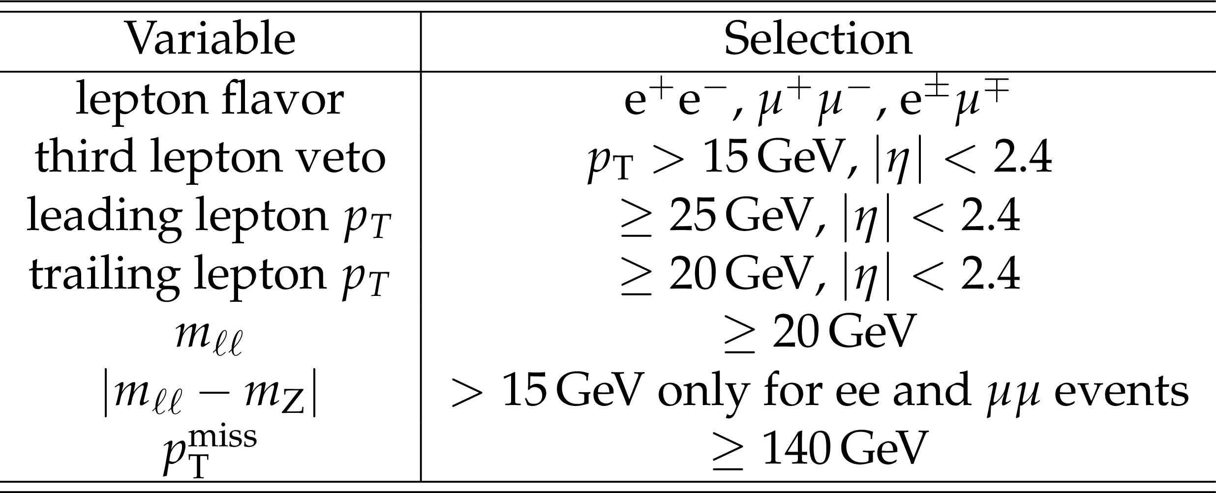
png pdf	Table 1: Definition of the baseline selection used in the searches for chargino pair production and top squark pair production.
png pdf	Table 2: Definition of the signal regions for the chargino search as a function of the b jet multiplicity, ISR jet requirement, and the ${{p_{\mathrm {T}}} ^\text {miss}}$ value. Also shown are the control regions with b-tagged jets used for the normalization of the $\mathrm{ t \bar{t} }$ and tW backgrounds. Each of the regions is further divided in seven ${M_{\text {T2}}(\ell \ell)}$ bins.
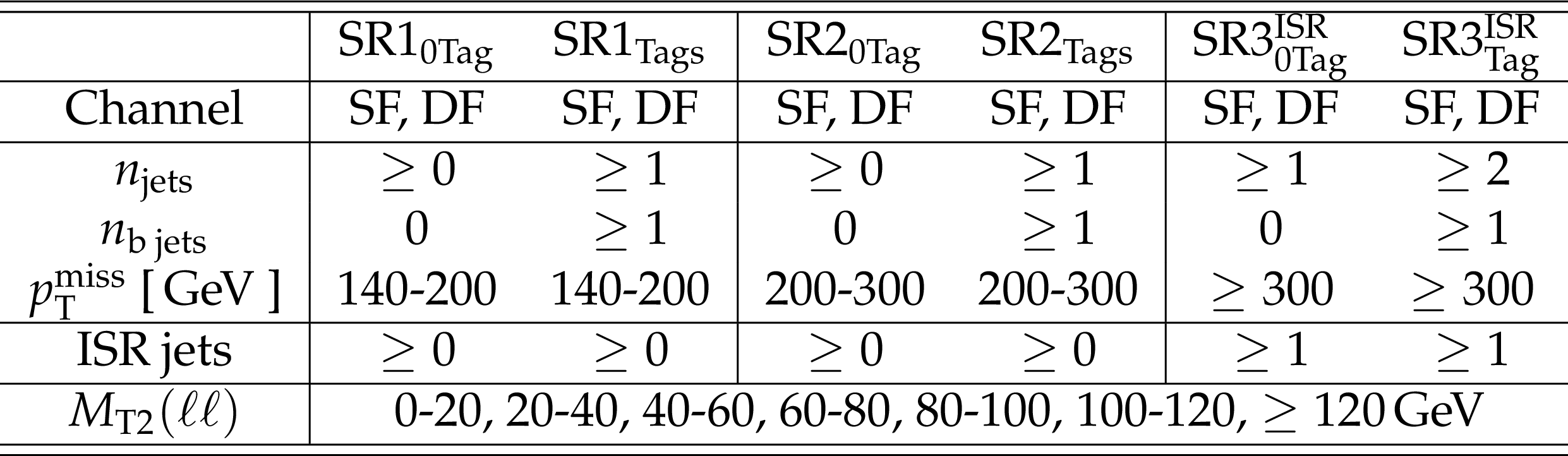
png pdf	Table 3: Definition of the signal regions for the top squark production search as a function of the b jet multiplicity, ISR jet requirement, and ${{p_{\mathrm {T}}} ^\text {miss}}$ value. Each of the regions is further divided in seven ${M_{\text {T2}}(\ell \ell)}$ bins.
png pdf	Table 4: Summary of the normalization scale factors for $\mathrm{ t \bar{t} }$ Z, WZ, and ZZ backgrounds in the signal regions used for the chargino (a) and top squark (b) searches. Uncertainties include the statistical uncertainties on data and simulated events, and the systematic uncertainties on the purity on the control regions.
png pdf	Table 5: Size of systematic uncertainties in the predicted yields for SM processes. The first column shows the range of the uncertainties in the global background normalization across the different signal regions, while the second one gives the effect on the ${M_{\text {T2}}(\ell \ell)}$ shape.
png pdf	Table 6: Observed and expected yields of DF events in the signal regions for the chargino search. The quoted uncertainty on the background predictions includes statistical and systematic contributions.
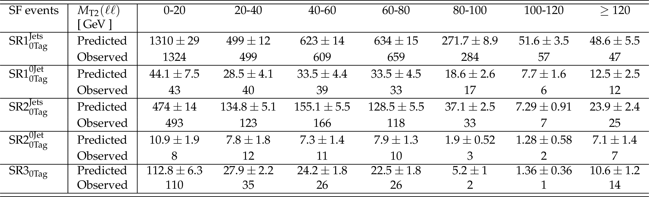
png pdf	Table 7: Observed and expected yields of SF events in the signal regions for the chargino search. The quoted uncertainty on the background predictions includes statistical and systematic contributions.
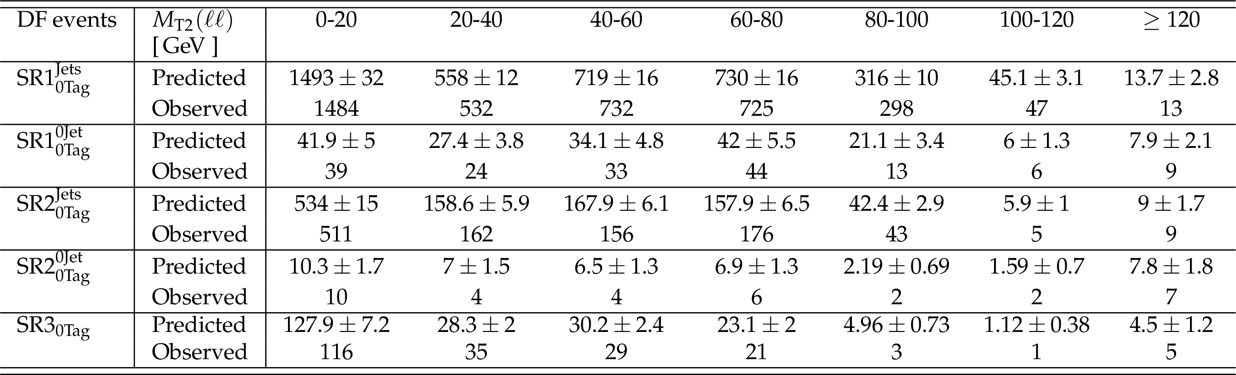
png pdf	Table 8: Observed and expected yields of DF events in the signal regions for the top squark search. The quoted uncertainty on the background predictions includes statistical and systematic contributions.
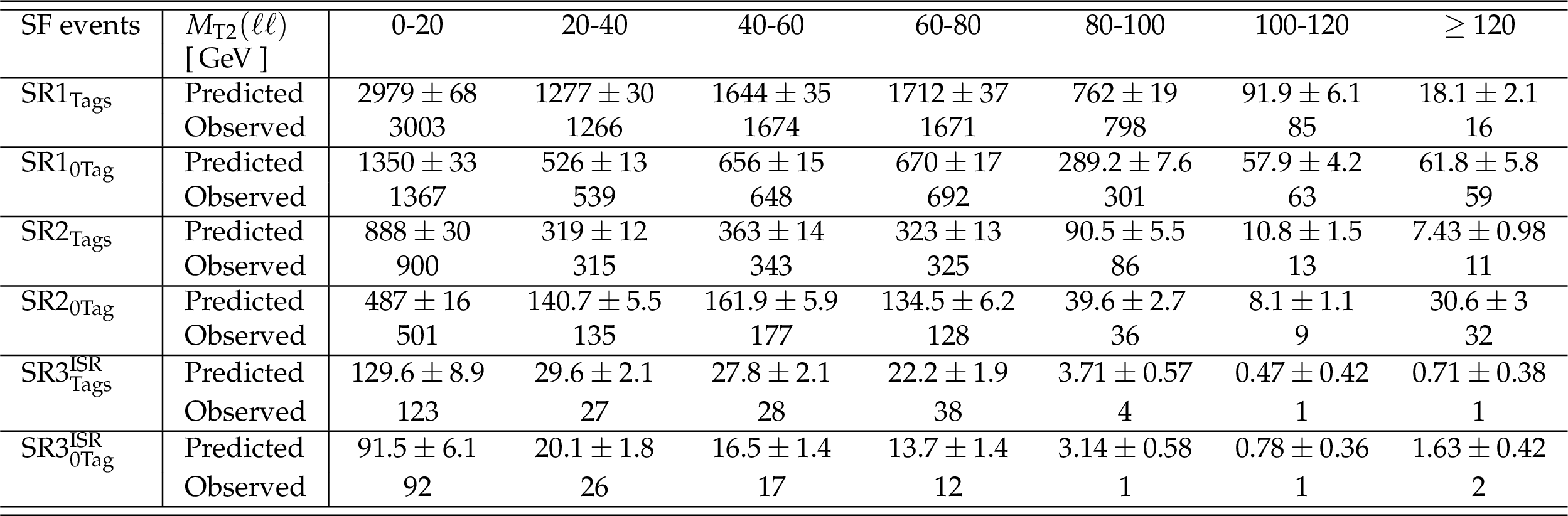
png pdf	Table 9: Observed and expected yields of SF events in the signal regions for the top squark search. The quoted uncertainty on the background predictions includes statistical and systematic contributions.

Summary

A search has been presented for new physics in events with two oppositely charged isolated leptons and missing transverse momentum in 35.9 fb

$^{-1}$ of proton-proton collision data collected by the CMS detector during the 2016 run of the LHC operation at a center-of-mass energy of 13 TeV. No evidence for a deviation with respect to SM predictions was observed in data, and the results have been used to set upper limits on the cross section of supersymmetric particle production for several simplified supersymmetric model spectra.

The chargino pair production has been investigated in two possible decay modes. If the chargino is assumed to undergo a cascade decay through sleptons, an exclusion region in the (

$m_{\tilde{\chi}^{\pm}_1}, m_{\tilde{\chi}^0_1}$ ) plane can be derived, extending till chargino masses of 800 GeV and neutralino masses of 320 GeV. These are the most stringent limits on this model to date. For chargino decays into a neutralino and a W boson, limits on production cross section have been derived assuming a neutralino mass of 1 GeV, and chargino masses in the range 170-200 GeV have been excluded.

Top squark pair production was also tested, with a focus on compressed decay modes. A model with the top squark decaying into a top quark and a neutralino was considered. In the region where

$m_{\mathrm{W}} < m_{\tilde{\mathrm{t}}}-m_{\tilde{\chi}^0_1} \lesssim m_{\mathrm{t}}$ , top squark masses are excluded up to about 420 GeV. An alternative model has also been considered, where the top squark decays into a chargino and a bottom quark, with the chargino subsequently decaying into a W boson and the lightest neutralino. The results extend the previous exclusion region in the dilepton channel [27] in the compressed region where 175

$\lesssim m_{\tilde{\mathrm{t}}}-m_{\tilde{\chi}^0_1} \lesssim$ 225 GeV up to a top squark mass of about 500 GeV.

References
1	G. Bertone, D. Hooper, and J. Silk	Particle dark matter: evidence, candidates and constraints	PR 405 (2005) 279	0404175
2	J. L. Feng	Dark matter candidates from particle physics and methods of detection	Ann. Rev. Astron. Astrophys. 48 (2010) 495	1003.0904
3	T. A. Porter, R. P. Johnson, and P. W. Graham	Dark matter searches with astroparticle data	Ann. Rev. Astron. Astrophys. 49 (2011) 155	1104.2836
4	P. Ramond	Dual theory for free fermions	PRD 3 (1971) 2415
5	Y. A. Golfand and E. P. Likhtman	Extension of the algebra of Poincar $\'e$ group generators and violation of P invariance	JEPTL 13 (1971)323
6	A. Neveu and J. H. Schwarz	Factorizable dual model of pions	NPB 31 (1971) 86
7	D. V. Volkov and V. P. Akulov	Possible universal neutrino interaction	JEPTL 16 (1972)438
8	J. Wess and B. Zumino	A Lagrangian model invariant under supergauge transformations	PLB 49 (1974) 52
9	J. Wess and B. Zumino	Supergauge transformations in four dimensions	NPB 70 (1974) 39
10	P. Fayet	Supergauge invariant extension of the Higgs mechanism and a model for the electron and its neutrino	NPB 90 (1975) 104
11	Nilles, Hans Peter	Supersymmetry, supergravity and particle physics	Phys. Rep. 110 (1984) 1
12	G. ’t Hooft	Naturalness, chiral symmetry, and spontaneous chiral symmetry breaking	NATO Sci. Ser. B 59 (1980) 135
13	E. Witten	Dynamical breaking of supersymmetry	NPB 188 (1981) 513
14	S. Dimopoulos and H. Georgi	Softly broken supersymmetry and SU(5)	NPB 193 (1981) 150
15	R. K. Kaul and P. Majumdar	Cancellation of quadratically divergent mass corrections in globally supersymmetric spontaneously broken gauge theories	NPB 199 (1982) 36
16	G. R. Farrar and P. Fayet	Phenomenology of the Production, Decay, and Detection of New Hadronic States Associated with Supersymmetry	PLB 76 (1978) 575
17	CMS Collaboration	The CMS experiment at the CERN LHC	JINST 3 (2008) S08004	CMS-00-001
18	J. Alwall, P. Schuster, and N. Toro	Simplified models for a first characterization of new physics at the LHC	PRD 79 (2009) 075020	0810.3921
19	J. Alwall, M.-P. Le, M. Lisanti, and J. G. Wacker	Model-independent jets plus missing energy searches	PRD 79 (2009) 015005	0809.3264
20	D. Alves et al.	Simplified models for LHC new physics searches	JPG 39 (2012) 105005	1105.2838
21	CMS Collaboration	Searches for electroweak production of charginos, neutralinos, and sleptons decaying to leptons and W, Z, and Higgs bosons in pp collisions at 8 TeV	EPJC 74 (2014) 3036
22	ATLAS Collaboration	Search for direct production of charginos, neutralinos and sleptons in final states with two leptons and missing transverse momentum in pp collisions at $\sqrt{s} =$ 8 TeV with the ATLAS detector	JHEP 1405 (2014) 071
23	ATLAS Collaboration	Search for the direct production of charginos, neutralinos and staus in final states with at least two hadronically decaying taus and missing transverse momentum in pp collisions at $\sqrt{s} =$ 8 TeV with the ATLAS detector	JHEP 1410 (2014) 096
24	ATLAS Collaboration	Search for the electroweak production of supersymmetric particles in $\sqrt{s} =$ 8 TeV pp collisions with the ATLAS detector	PRD 93 (2016) 052002
25	ATLAS Collaboration	Search for the direct production of charginos and neutralinos in $\sqrt{s} =$ 13 TeV pp collisions with the atlas detector	Submitted to EPJC	1708.07875
26	ATLAS Collaboration	Search for electroweak production of supersymmetric states in scenarios with compressed mass spectra at $\sqrt{s} =$ 13 TeV with the atlas detector	Submitted to PRD	1712.08119
27	CMS Collaboration	Search for top squarks and dark matter particles in opposite-charge dilepton final states at $\sqrt{s} =$ 13 TeV	PRD 97 (2018) 032009	CMS-SUS-17-001 1711.00752
28	CMS Collaboration	Search for top squark pair production in pp collisions at $\sqrt{s} =$ 13 TeV using single lepton events	JHEP 10 (2017) 019	CMS-SUS-16-051 1706.04402
29	CMS Collaboration	Search for direct production of supersymmetric partners of the top quark in the all-jets final state in proton-proton collisions at $\sqrt{s} =$ 13 TeV	JHEP 10 (2017) 005	CMS-SUS-16-049 1707.03316
30	ATLAS Collaboration	Search for a scalar partner of the top quark in the jets plus missing transverse momentum final state at $\sqrt{s} =$ 13 TeV TeV with the ATLAS detector	JHEP 12 (2017) 085	1709.04183
31	ATLAS Collaboration	Search for top-squark pair production in final states with one lepton, jets, and missing transverse momentum using $36 fb$ ^{-1} of $\sqrt{s} =$ 13 TeV pp collision data with the ATLAS detector	Submitted to JHEP	1711.11520
32	ATLAS Collaboration	Search for direct top squark pair production in final states with two leptons in $\sqrt{s} =$ 13 TeV pp collisions with the ATLAS detector	EPJC 77 (2017) 898	1708.03247
33	CMS Collaboration	The CMS trigger system	JINST 12 (2017) P01020	CMS-TRG-12-001 1609.02366
34	P. Nason	A new method for combining NLO QCD with shower Monte Carlo algorithms	JHEP 11 (2004) 040	0409146
35	S. Frixione, P. Nason, and C. Oleari	Matching NLO QCD computations with parton shower simulations: the POWHEG method	JHEP 11 (2007) 070	0709.2092
36	S. Alioli, P. Nason, C. Oleari, and E. Re	A general framework for implementing NLO calculations in shower Monte Carlo programs: the POWHEG BOX	JHEP 06 (2010) 043	1002.2581
37	M. Czakon and A. Mitov	Top++: A Program for the Calculation of the Top-Pair Cross-Section at Hadron Colliders	Comput.Phys.Commun. 185 (2014) 2930	1112.5675
38	E. Re	Single-top Wt-channel production matched with parton showers using the POWHEG method	EPJC 71 (2011) 1547	1009.2450
39	T. Melia, P. Nason, R. Rontsch, and G. Zanderighi	WW, WZ and ZZ production in the POWHEG BOX	JHEP 11 (2011) 078	1107.5051
40	P. Nason and G. Zanderighi	WW, WZ and ZZ production in the POWHEG-BOX-V2	EPJC 74 (2014) 2702	1311.1365
41	J. M. Campbell and R. K. Ellis	MCFM for the Tevatron and the LHC	NPPS 205 (2010) 10	1007.3492
42	J. Alwall et al.	The automated computation of tree-level and next-to-leading order differential cross sections, and their matching to parton shower simulations	JHEP 07 (2014) 079	1405.0301
43	R. Gavin, Y. Li, F. Petriello, and S. Quackenbush	FEWZ 2.0: A code for hadronic Z production at next-to-next-to-leading order	CPC 182 (2011) 2388	1011.3540
44	M. V. Garzelli, A. Kardos, C. G. Papadopoulos, and Z. Trocsanyi	$\mathrm{t\bar{t}}$ W $^{\pm}$ and $\mathrm{t\bar{t}}$ Z hadroproduction at NLO accuracy in QCD with parton shower and hadronization effects	JHEP 11 (2012) 056	1208.2665
45	LHC Higgs Cross Section Working Group Collaboration	Handbook of LHC Higgs Cross Sections: 3. Higgs Properties		1307.1347
46	W. Beenakker et al.	Production of Charginos, Neutralinos, and Sleptons at Hadron Colliders	PRL 83 (1999) 3780	hep-ph/9906298
47	B. Fuks, M. Klasen, D. R. Lamprea, and M. Rothering	Gaugino production in proton-proton collisions at a center-of-mass energy of 8 TeV	JHEP 10 (2012) 081	1207.2159
48	B. Fuks, M. Klasen, D. R. Lamprea, and M. Rothering	Precision predictions for electroweak superpartner production at hadron colliders with $\sc$ Resummino	EPJC 73 (2013) 2480	1304.0790
49	W. Beenakker, R. Hopker, M. Spira, and P. M. Zerwas	Squark and gluino production at hadron colliders	NPB 492 (1997) 51	hep-ph/9610490
50	A. Kulesza and L. Motyka	Threshold resummation for squark-antisquark and gluino-pair production at the LHC	PRL 102 (2009) 111802	0807.2405
51	A. Kulesza and L. Motyka	Soft gluon resummation for the production of gluino-gluino and squark-antisquark pairs at the LHC	PRD 80 (2009) 095004	0905.4749
52	W. Beenakker et al.	Soft-gluon resummation for squark and gluino hadroproduction	JHEP 12 (2009) 041	0909.4418
53	W. Beenakker et al.	Squark and Gluino Hadroproduction	Int. J. Mod. Phys. A 26 (2011) 2637	1105.1110
54	C. Borschensky et al.	Squark and gluino production cross sections in pp collisions at $\sqrt{s} =$ 13, 14, 33 and 100 TeV	EPJC 74 (2014) 3174	1407.5066
55	N. Collaboration	Parton distributions for the LHC Run II	JHEP 04 (2015) 040	1410.8849
56	T. Sjöstrand et al.	An Introduction to PYTHIA 8.2	CPC 191 (2015) 159--177	1410.3012
57	C. Collaboration	Event generator tunes obtained from underlying event and multiparton scattering measurements	EPJC 76 (2016) 155	1512.00815
58	A. Kalogeropoulos and J. Alwall	The SysCalc code: A tool to derive theoretical systematic uncertainties		1801.08401
59	GEANT4 Collaboration	GEANT4: A simulation toolkit	NIMA506 (2003) 250
60	CMS Collaboration	The fast simulation of the CMS detector at LHC	J.Phys.Conf.Ser. 331 (2011) 032049
61	CMS Collaboration	Search for top-squark pair production in the single-lepton final state in pp collisions at sqrt(s) = 8 TeV	EPJC 73 (2013) 2677	CMS-SUS-13-011 1308.1586
62	CMS Collaboration	Particle-flow reconstruction and global event description with the CMS detector	JINST 12 (2017) P10003	CMS-PRF-14-001 1706.04965
63	M. Cacciari, G. P. Salam, and G. Soyez	The anti- $k_t$ jet clustering algorithm	JHEP 04 (2008) 063	0802.1189
64	M. Cacciari, G. P. Salam, and G. Soyez	FastJet user manual	EPJC 72 (2012) 1896	1111.6097
65	CMS Collaboration	Performance of electron reconstruction and selection with the CMS detector in proton-proton collisions at $\sqrt{s} =$ 8 TeV	JINST 10 (2015) P06005	CMS-EGM-13-001 1502.02701
66	CMS Collaboration	Performance of CMS muon reconstruction in $pp$ collision events at $\sqrt{s} =$ 7 TeV	JINST 7 (2012) P10002	CMS-MUO-10-004 1206.4071
67	CMS Collaboration	Jet energy scale and resolution in the CMS experiment in pp collisions at 8 TeV	JINST 12 (2017) P02014	CMS-JME-13-004 1607.03663
68	CMS Collaboration	Identification of heavy-flavour jets with the CMS detector in pp collisions at 13 TeV	Submitted to \it JINST	CMS-BTV-16-002 1712.07158
69	C. G. Lester and D. J. Summers	Measuring masses of semiinvisibly decaying particles pair produced at hadron colliders	PLB463 (1999) 99--103	hep-ph/9906349
70	CMS Collaboration	CMS Luminosity Measurements at 13 TeV - Winter 2017 update	CMS-PAS-LUM-17-001	CMS-PAS-LUM-17-001
71	CMS Collaboration	Measurement of differential cross sections for top quark pair production using the lepton+jets final state in proton-proton collisions at 13 TeV	PRD 95 (2017) 092001	CMS-TOP-16-008 1610.04191
72	CMS Collaboration	Measurement of the differential cross section for top quark pair production in pp collisions at $\sqrt{s} =$ 8 TeV	EPJC 75 (2015) 542	CMS-TOP-12-028 1505.04480
73	CMS Collaboration	Measurement of the $\mathrm{t\bar{t}}$ production cross section in the all-jets final state in pp collisions at $\sqrt{s} =$ 8 TeV	EPJC 76 (2016) 128	CMS-TOP-14-018 1509.06076
74	A. Read	Presentation of search results: the CLs technique	JPG 28 (2002) 2693
75	T. Junk	Confidence level computation for combining searches with small statistics	NIMA 434 (1999) 435	9902006
76	G. Cowan, K. Cranmer, E. Gross, and O. Vitells	Asymptotic formulae for likelihood-based tests of new physics	EPJC 71 (2011) 1554	1007.1727