

Compact Muon Solenoid
LHC, CERN
| CMS-PAS-HIG-16-041 | ||
| Measurements of properties of the Higgs boson in the four-lepton final state at $\sqrt{s}= $ 13 TeV | ||
| CMS Collaboration | ||
| March 2017 | ||
| Abstract: Properties of the Higgs boson are measured in the $\mathrm{H}\rightarrow{\rm Z}{\rm Z}\rightarrow4\ell$ ($\ell={\rm e},\mu$) decay channel. A data sample of proton-proton collisions at a center-of-mass energy of 13 TeV is used, corresponding to an integrated luminosity of 35.9 fb$^{-1}$ recorded by the CMS detector at the LHC. The signal-strength modifier $\mu$, defined as the production cross section of the Higgs boson times its branching fraction to four leptons relative to the standard model expectation, is measured to be $ \mu = $ 1.05$^{+0.19}_{-0.17}$ at $m_{\mathrm{H}} = $ 125.09 GeV. The signal-strength modifiers for the main Higgs boson production modes have also been constrained. The mass is measured to be $ m_{ \mathrm { H } } = $ 125.26 $ \pm $ 0.21 GeV and the width is constrained using on-shell production to be $ \Gamma_{\mathrm{H}}< $ 1.10 GeV, at 95% CL. The fiducial cross section is measured to be 2.90$^{+0.48}_{-0.44}$ (stat.) $^{+0.27}_{-0.22}$ (sys.) fb, which is compatible with the standard model prediction of 2.72 $\pm$ 0.14 fb. Differential cross sections as a function of the $p_{\rm T}$ of the Higgs boson, the number of associated jets, and the $p_{\rm T}$ of the leading associated jet are determined. | ||
|
Links:
CDS record (PDF) ;
inSPIRE record ;
CADI line (restricted) ;
These preliminary results are superseded in this paper, JHEP 11 (2017) 047. The superseded preliminary plots can be found here. |
||
| Figures & Tables | Summary | Additional Figures | References | CMS Publications |
|---|
| Figures | |
png pdf |
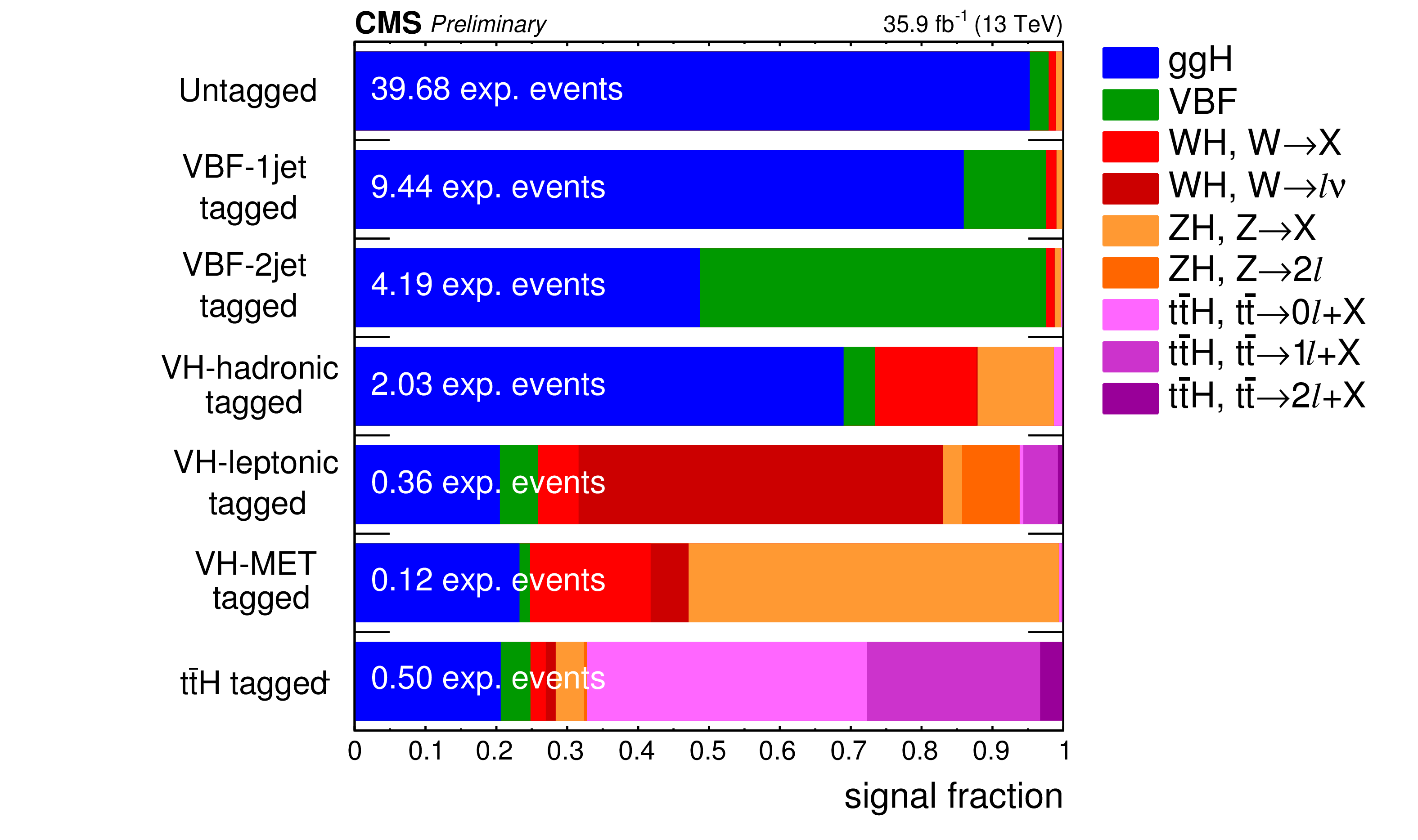
Figure 1:
Signal relative purity of the seven event categories in terms of the 5 main production mechanisms of the Higgs boson in a 118 $ < {m_{4\ell }}< $ 130 GeV window. The $ {\mathrm{ W } \mathrm{ H } }$, $ {\mathrm{ Z } \mathrm{ H } }$ and $ {\mathrm{ t } \bar{\mathrm{ t } }\mathrm{ H } }$ processes are split according to the decay of associated objects, whereby X denotes anything other than an electron or muon. |
png pdf |
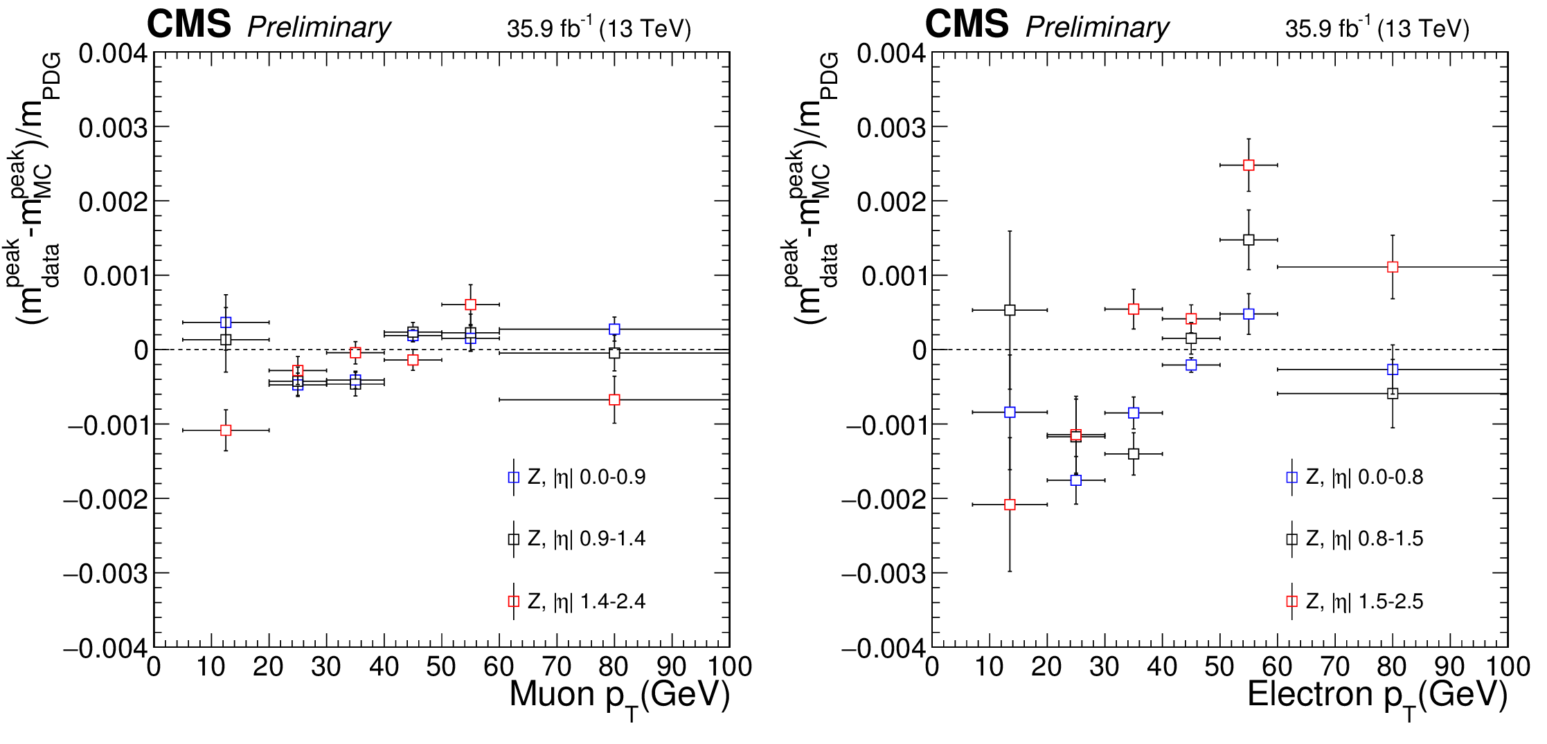
Figure 2:
Difference between the ${\rm Z}\rightarrow \ell \ell $ mass peak positions in data and simulation normalized by the nominal Z boson mass obtained as a function of the $ {p_{\mathrm {T}}} $ and $|\eta |$ of one of the leptons regardless of the second for muons (left) and electrons (right). |
png pdf |
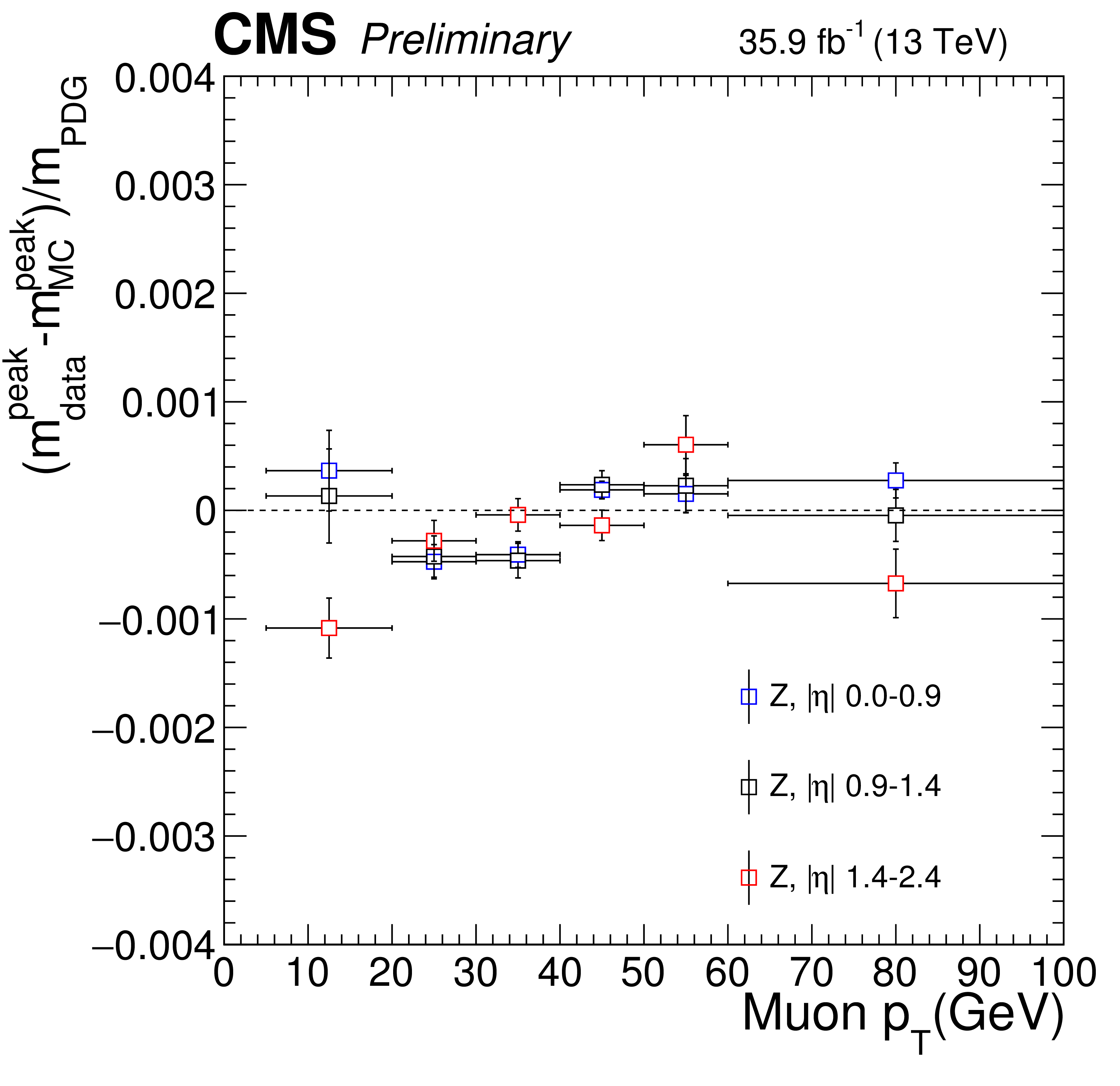
Figure 2-a:
Difference between the ${\rm Z}\rightarrow \ell \ell $ mass peak positions in data and simulation normalized by the nominal Z boson mass obtained as a function of the $ {p_{\mathrm {T}}} $ and $|\eta |$ of one of the leptons regardless of the second for muons. |
png pdf |
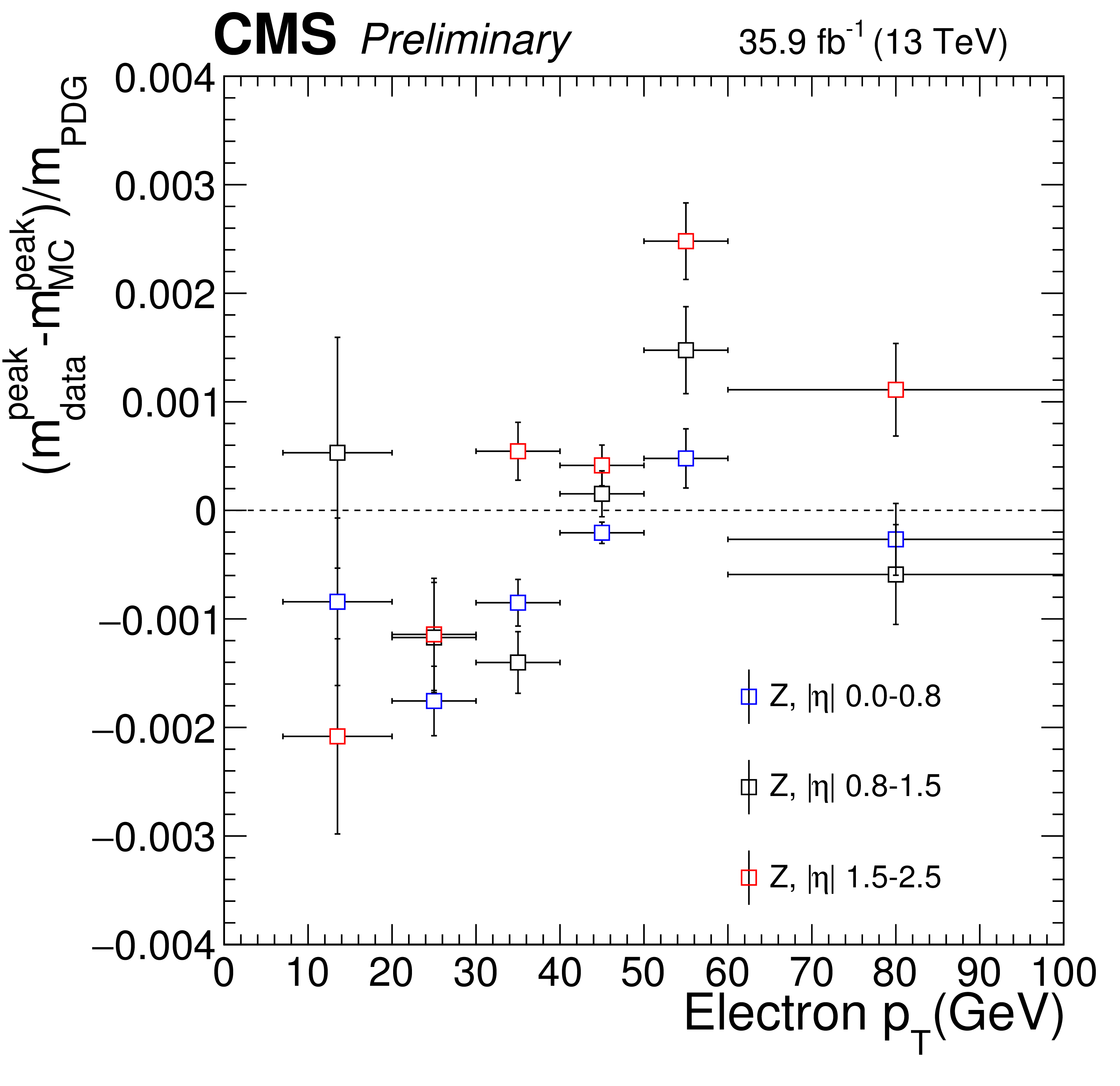
Figure 2-b:
Difference between the ${\rm Z}\rightarrow \ell \ell $ mass peak positions in data and simulation normalized by the nominal Z boson mass obtained as a function of the $ {p_{\mathrm {T}}} $ and $|\eta |$ of one of the leptons regardless of the second for electrons. |
png pdf |
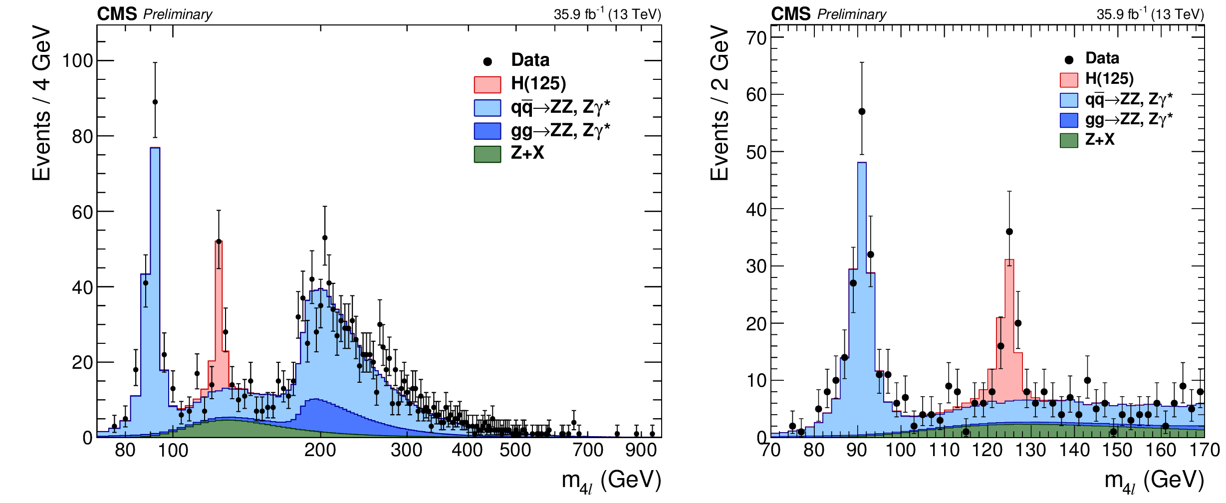
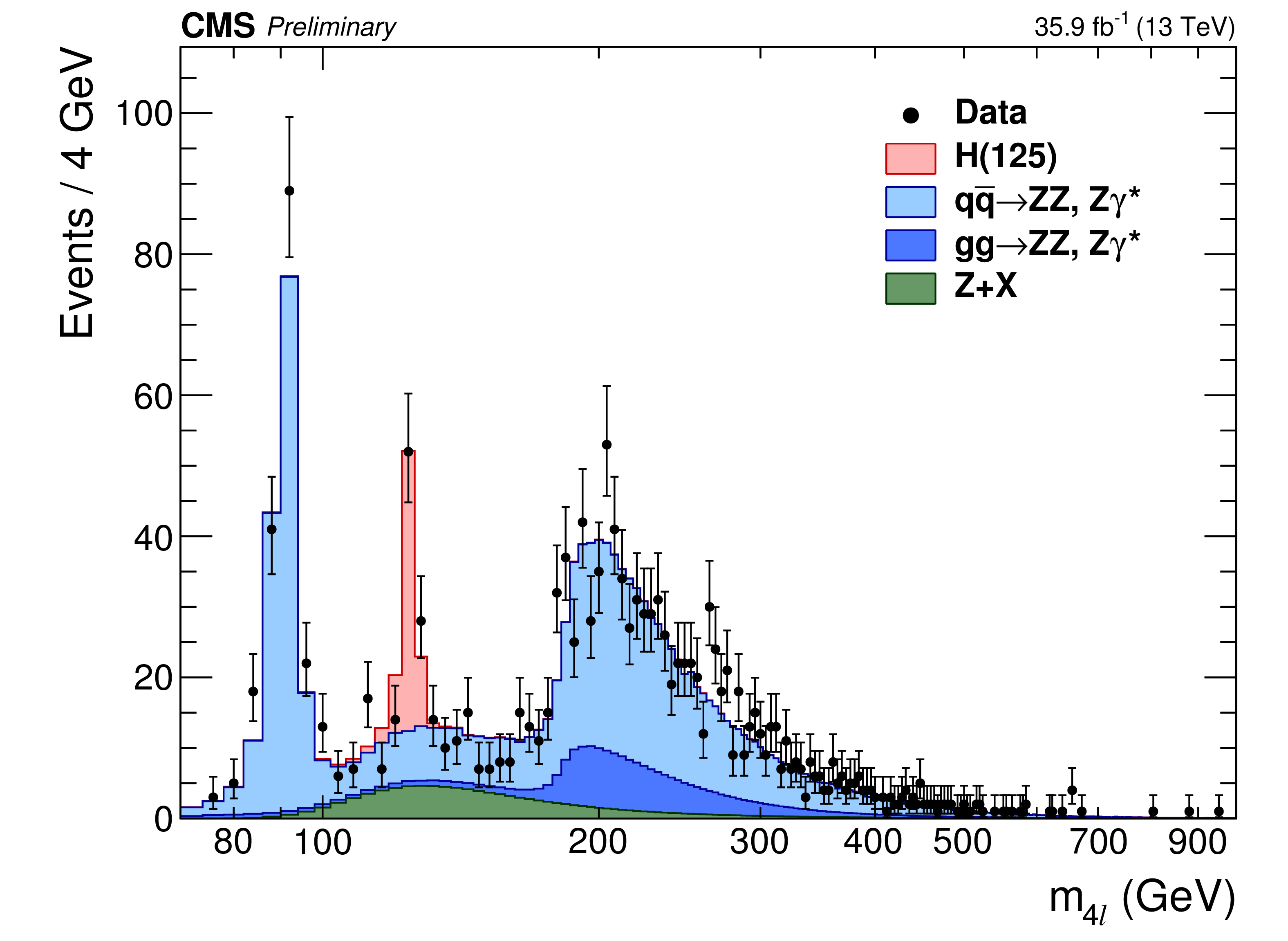
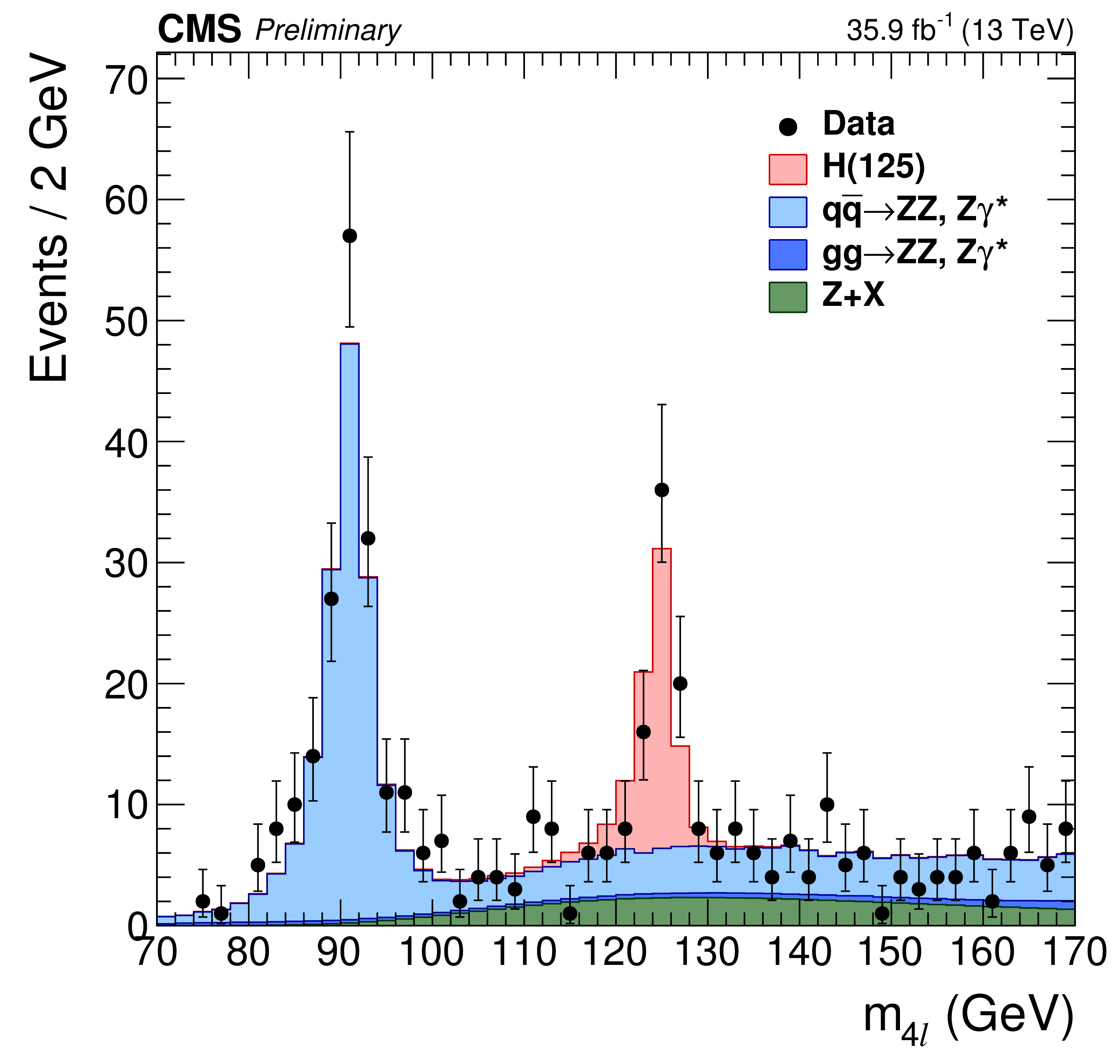
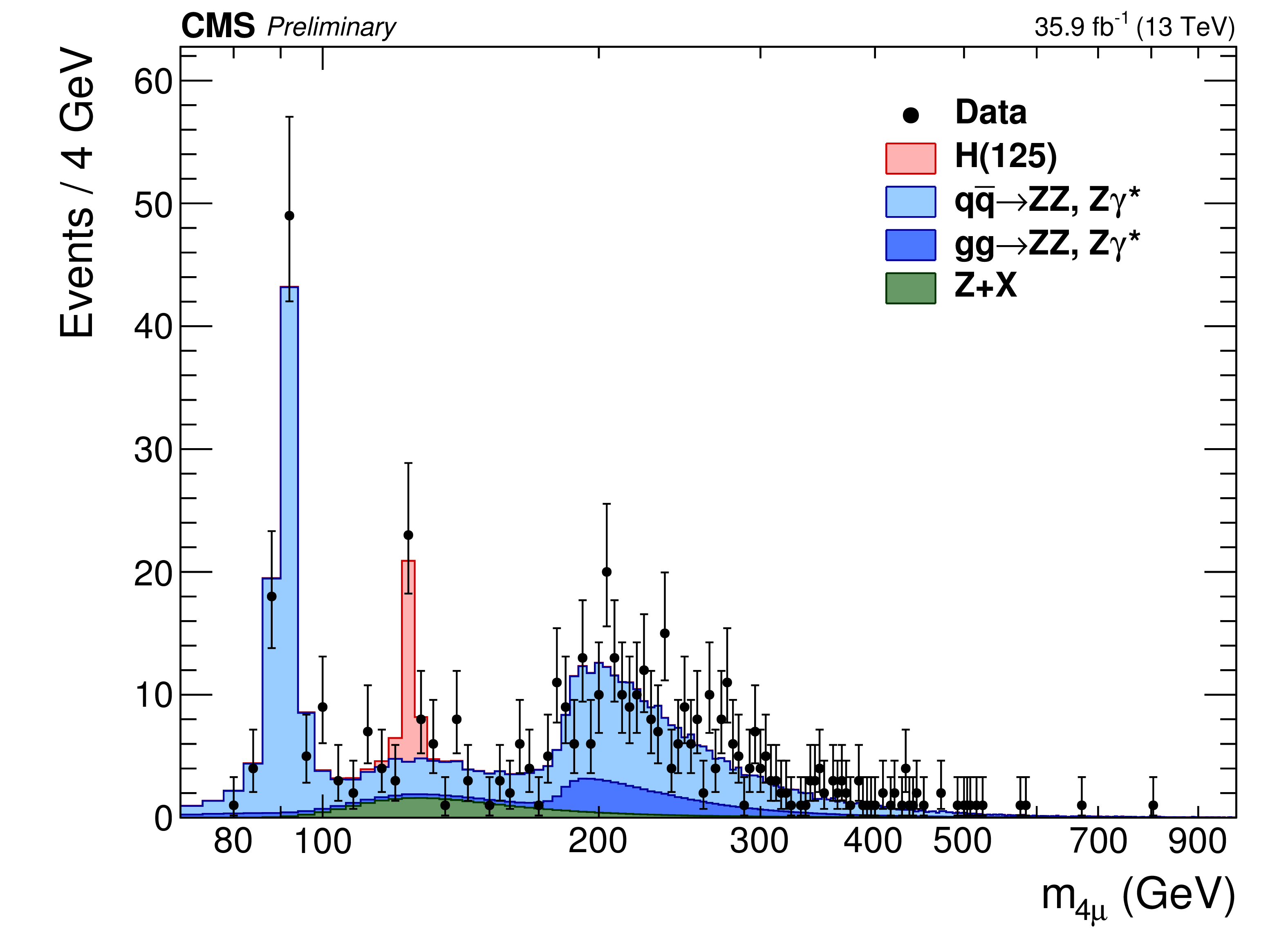
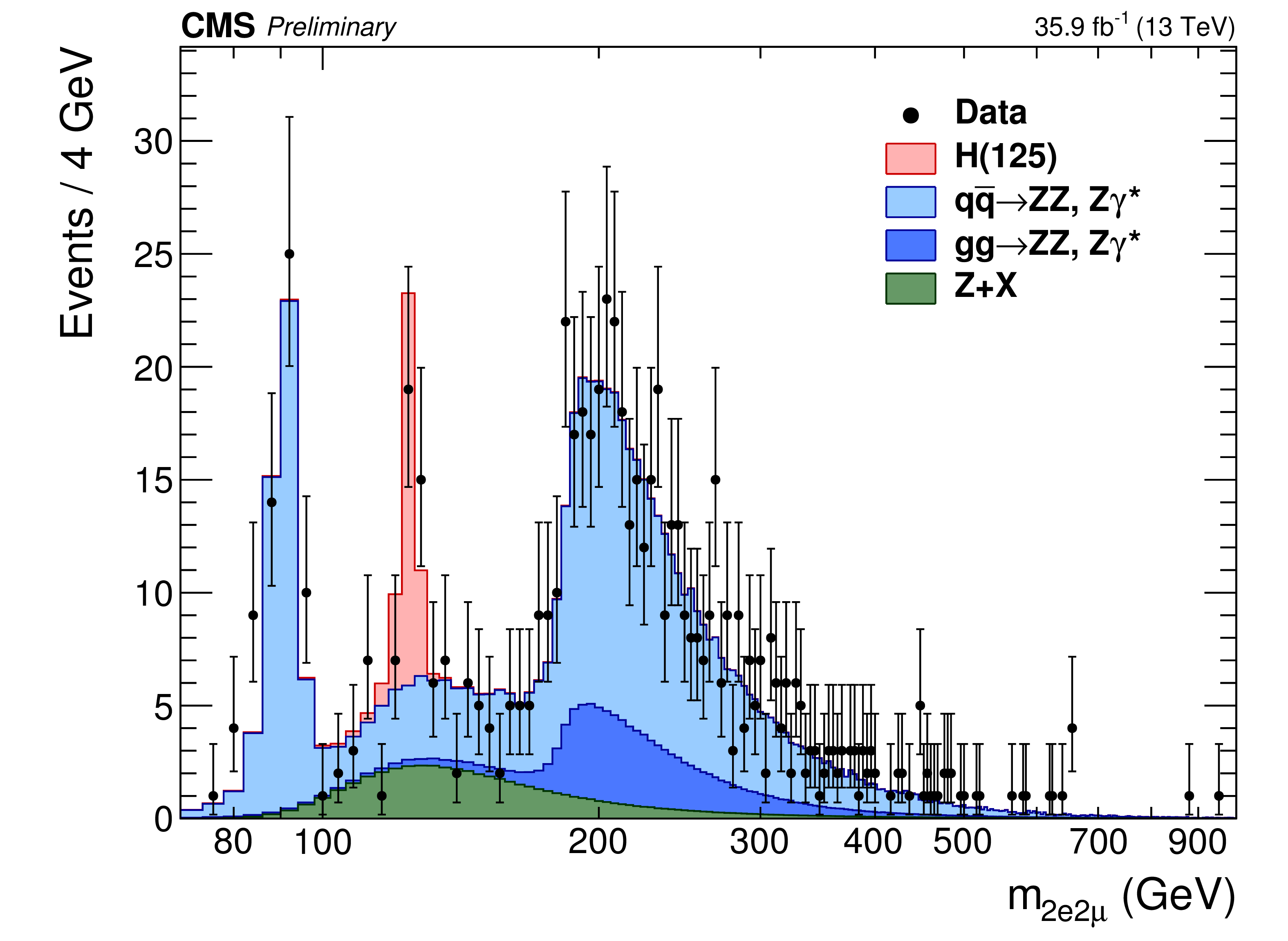
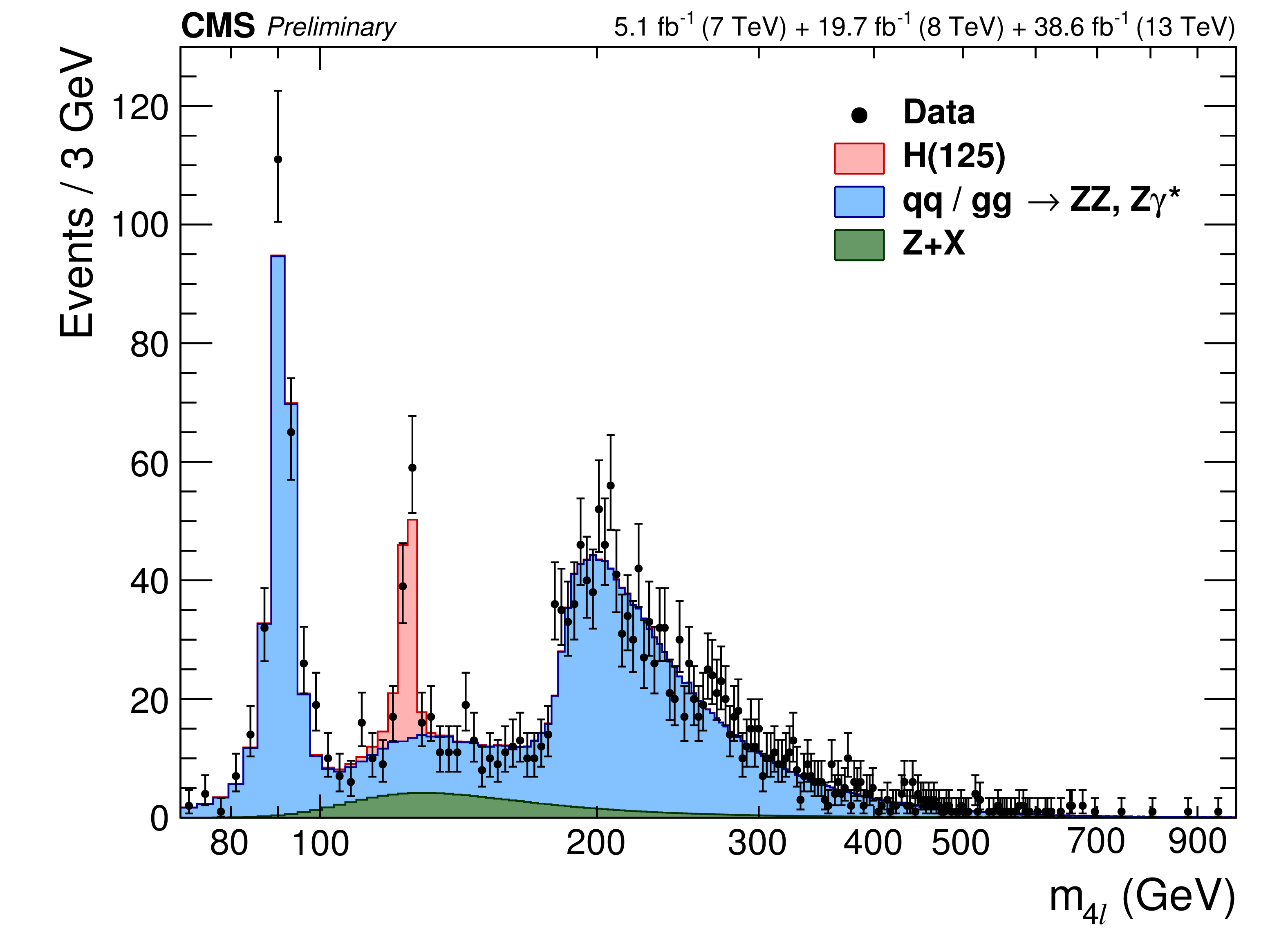
Figure 3:
Distribution of the four-lepton reconstructed invariant mass $ {m_{4\ell }}$ in the full mass range (left) and the low-mass range (right). Points with error bars represent the data and stacked histograms represent expected distributions. The SM Higgs boson signal with $ {m_{\mathrm{ H } }}=$ 125 GeV, denoted as H(125), and the ZZ backgrounds are normalized to the SM expectation, the Z+X background to the estimation from data. The order in perturbation theory used for the normalization of the irreducible backgrounds is described in Section 7.1. No events are observed with $ {m_{4\ell }} > $ 1 TeV. |
png pdf |
Figure 3-a:
Distribution of the four-lepton reconstructed invariant mass $ {m_{4\ell }}$ in the full mass range. Points with error bars represent the data and stacked histograms represent expected distributions. The SM Higgs boson signal with $ {m_{\mathrm{ H } }}=$ 125 GeV, denoted as H(125), and the ZZ backgrounds are normalized to the SM expectation, the Z+X background to the estimation from data. The order in perturbation theory used for the normalization of the irreducible backgrounds is described in Section 7.1. No events are observed with $ {m_{4\ell }} > $ 1 TeV. |
png pdf |
Figure 3-b:
Distribution of the four-lepton reconstructed invariant mass $ {m_{4\ell }}$ in the low-mass range. Points with error bars represent the data and stacked histograms represent expected distributions. The SM Higgs boson signal with $ {m_{\mathrm{ H } }}=$ 125 GeV, denoted as H(125), and the ZZ backgrounds are normalized to the SM expectation, the Z+X background to the estimation from data. The order in perturbation theory used for the normalization of the irreducible backgrounds is described in Section 7.1. |
png pdf |
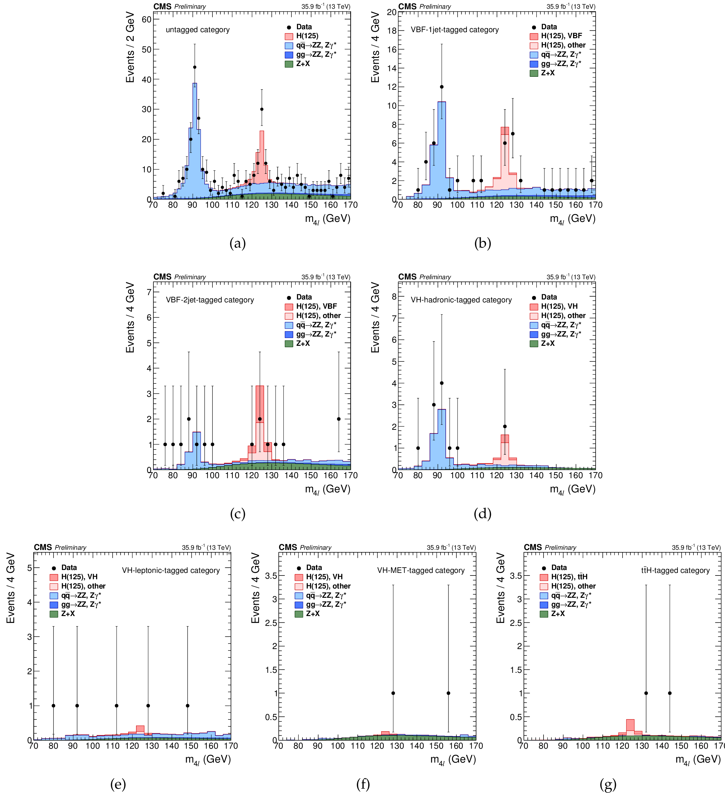
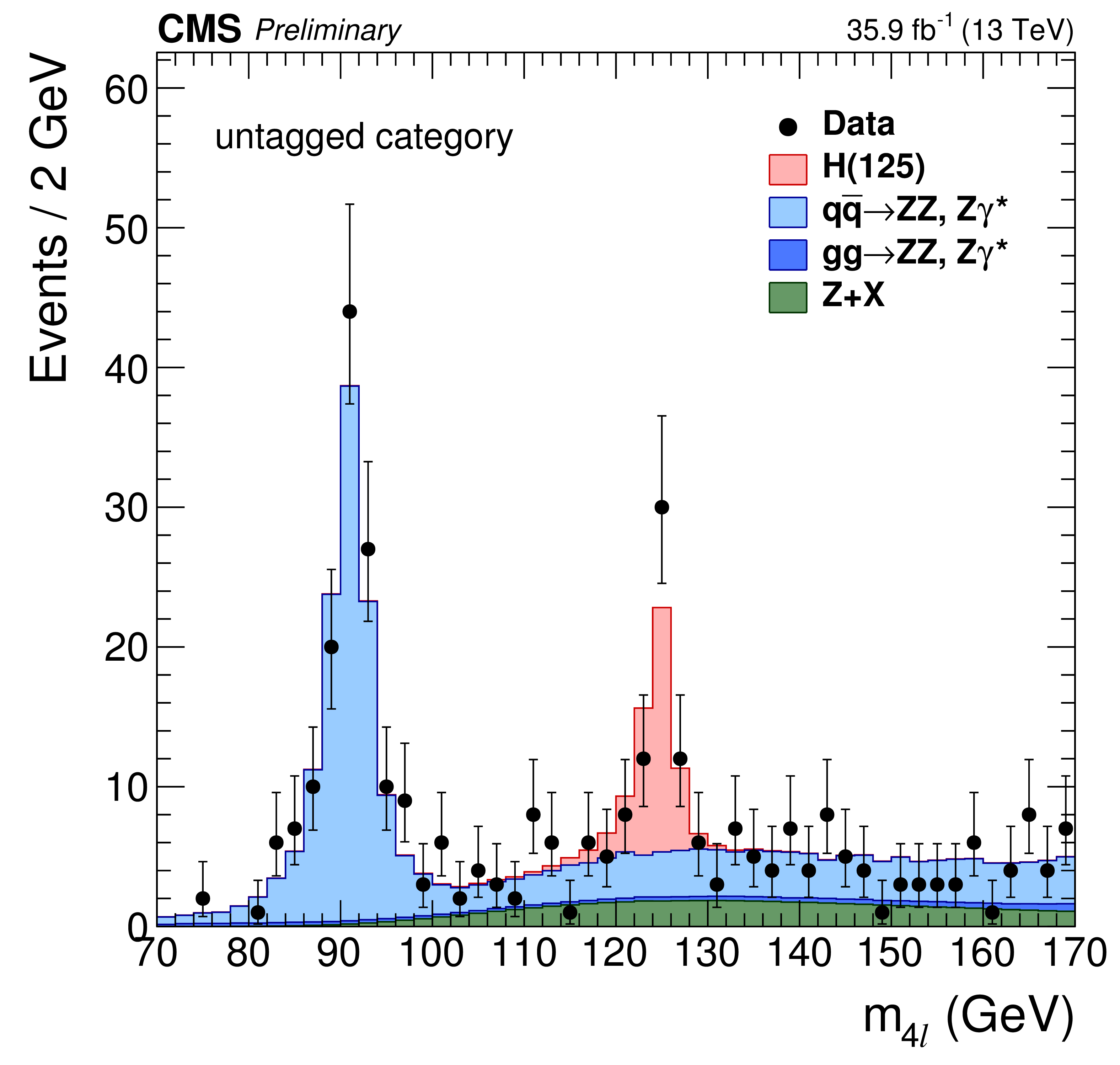
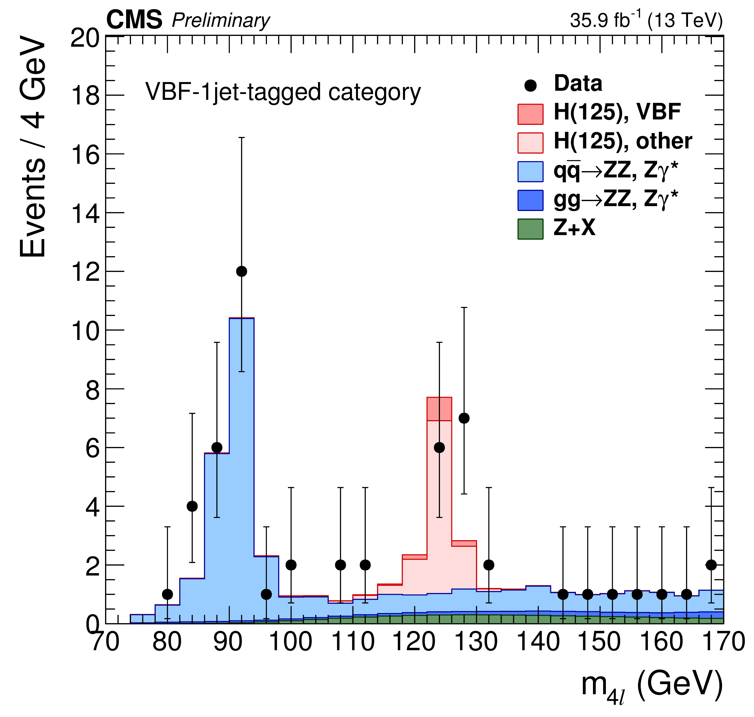
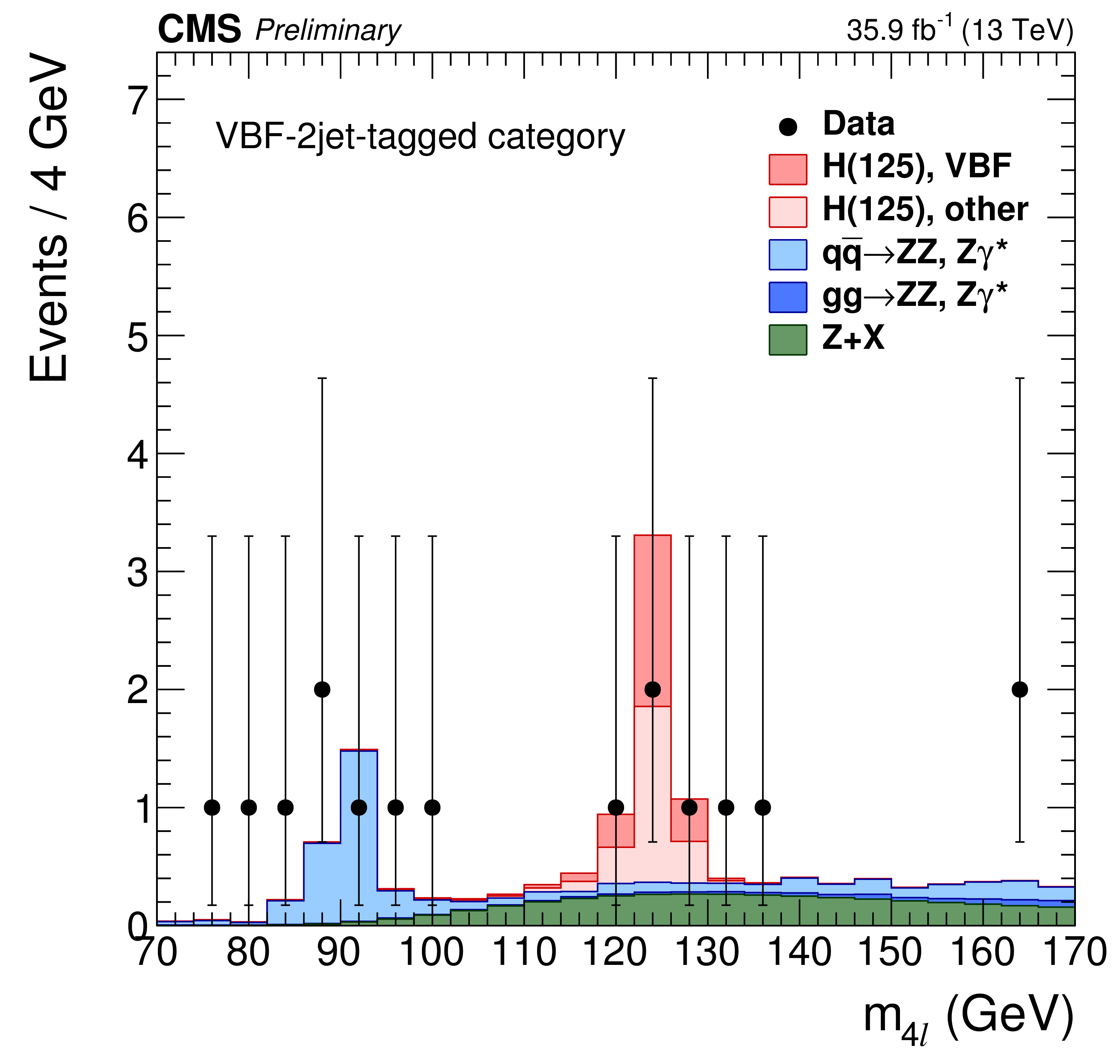
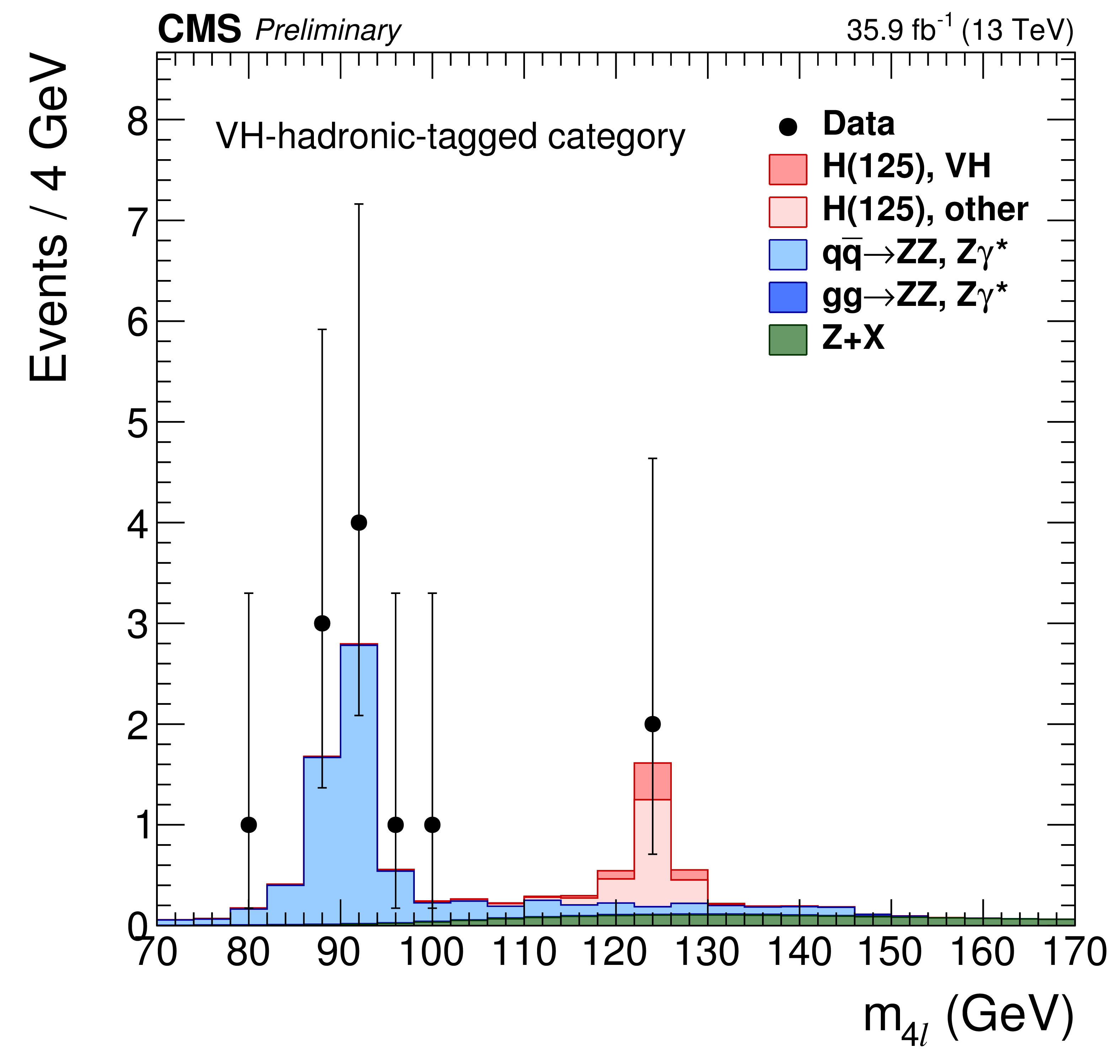
Figure 4:
Distribution of the four-lepton reconstructed mass in the seven event categories for the low-mass range. (a) untagged category (b) VBF-1jet-tagged category (c) VBF-2jet-tagged category (d) VH-hadronic-tagged category (e) VH-leptonic-tagged category (f) VH-MET-tagged category (g) ttH-tagged category. Points with error bars represent the data and stacked histograms represent expected distributions. The SM Higgs boson signal with $ {m_{\mathrm{ H } }}=$ 125 GeV, denoted as H(125), and the ZZ backgrounds are normalized to the SM expectation, the Z+X background to the estimation from data. For the categories other than the untagged category, the SM Higgs boson signal is separated into two components: the production mode which is targeted by the specific category, and other production modes which is always dominated by the gluon fusion process. The order in pertubation theory used for the normalization of the irreducible backgrounds is described in Section 7.1. |
png pdf |
Figure 4-a:
Distribution of the four-lepton reconstructed mass in the untagged category. Points with error bars represent the data and stacked histograms represent expected distributions. The SM Higgs boson signal with $ {m_{\mathrm{ H } }}=$ 125 GeV, denoted as H(125), and the ZZ backgrounds are normalized to the SM expectation, the Z+X background to the estimation from data. The order in pertubation theory used for the normalization of the irreducible backgrounds is described in Section 7.1. |
png pdf |
Figure 4-b:
Distribution of the four-lepton reconstructed mass in the VBF-1jet-tagged category. Points with error bars represent the data and stacked histograms represent expected distributions. The SM Higgs boson signal with $ {m_{\mathrm{ H } }}=$ 125 GeV, denoted as H(125), and the ZZ backgrounds are normalized to the SM expectation, the Z+X background to the estimation from data. The SM Higgs boson signal is separated into two components: the production mode which is targeted, and other production modes which is always dominated by the gluon fusion process. The order in pertubation theory used for the normalization of the irreducible backgrounds is described in Section 7.1. |
png pdf |
Figure 4-c:
Distribution of the four-lepton reconstructed mass in the VBF-2jet-tagged category. Points with error bars represent the data and stacked histograms represent expected distributions. The SM Higgs boson signal with $ {m_{\mathrm{ H } }}=$ 125 GeV, denoted as H(125), and the ZZ backgrounds are normalized to the SM expectation, the Z+X background to the estimation from data. The SM Higgs boson signal is separated into two components: the production mode which is targeted, and other production modes which is always dominated by the gluon fusion process. The order in pertubation theory used for the normalization of the irreducible backgrounds is described in Section 7.1. |
png pdf |
Figure 4-d:
Distribution of the four-lepton reconstructed mass in the VH-hadronic-tagged category. Points with error bars represent the data and stacked histograms represent expected distributions. The SM Higgs boson signal with $ {m_{\mathrm{ H } }}=$ 125 GeV, denoted as H(125), and the ZZ backgrounds are normalized to the SM expectation, the Z+X background to the estimation from data. The SM Higgs boson signal is separated into two components: the production mode which is targeted, and other production modes which is always dominated by the gluon fusion process. The order in pertubation theory used for the normalization of the irreducible backgrounds is described in Section 7.1. |
png pdf |
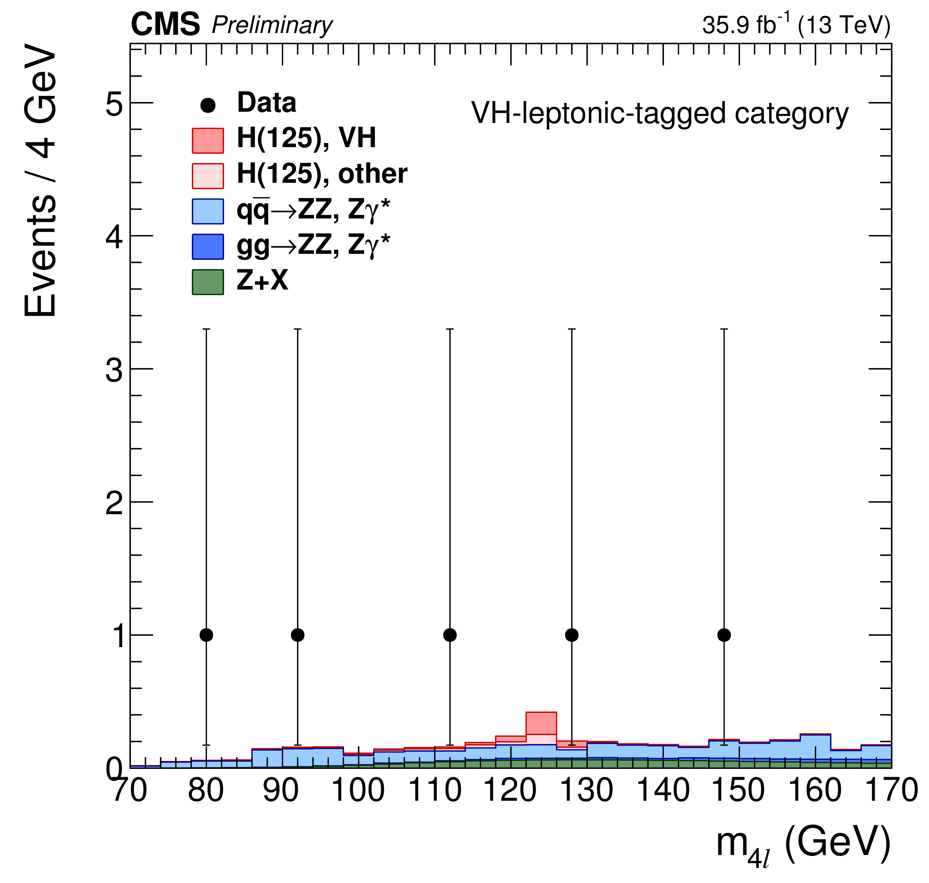
Figure 4-e:
Distribution of the four-lepton reconstructed mass in the VH-leptonic-tagged category. Points with error bars represent the data and stacked histograms represent expected distributions. The SM Higgs boson signal with $ {m_{\mathrm{ H } }}=$ 125 GeV, denoted as H(125), and the ZZ backgrounds are normalized to the SM expectation, the Z+X background to the estimation from data. The SM Higgs boson signal is separated into two components: the production mode which is targeted, and other production modes which is always dominated by the gluon fusion process. The order in pertubation theory used for the normalization of the irreducible backgrounds is described in Section 7.1. |
png pdf |
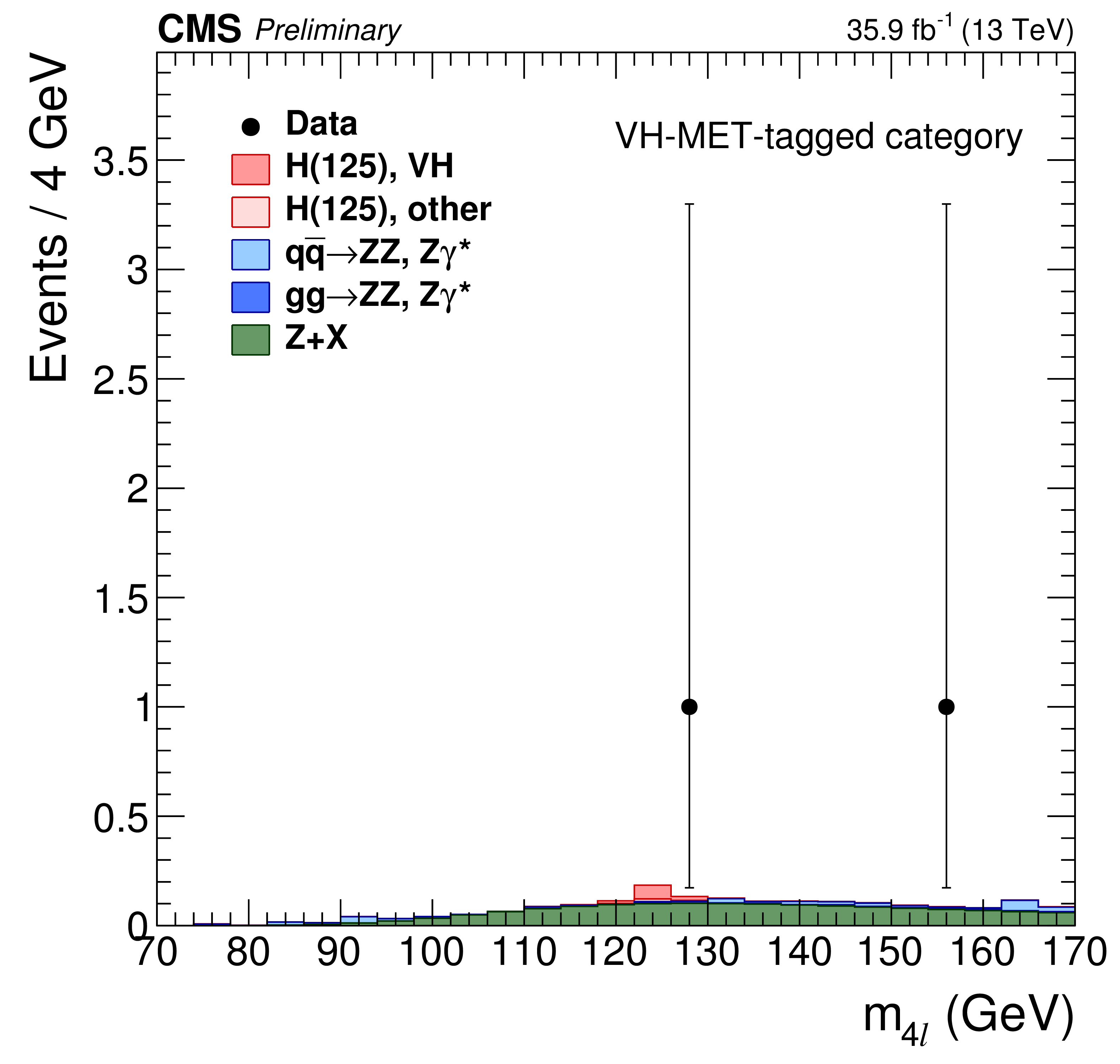
Figure 4-f:
Distribution of the four-lepton reconstructed mass in the VH-MET-tagged category. Points with error bars represent the data and stacked histograms represent expected distributions. The SM Higgs boson signal with $ {m_{\mathrm{ H } }}=$ 125 GeV, denoted as H(125), and the ZZ backgrounds are normalized to the SM expectation, the Z+X background to the estimation from data. The SM Higgs boson signal is separated into two components: the production mode which is targeted, and other production modes which is always dominated by the gluon fusion process. The order in pertubation theory used for the normalization of the irreducible backgrounds is described in Section 7.1. |
png pdf |
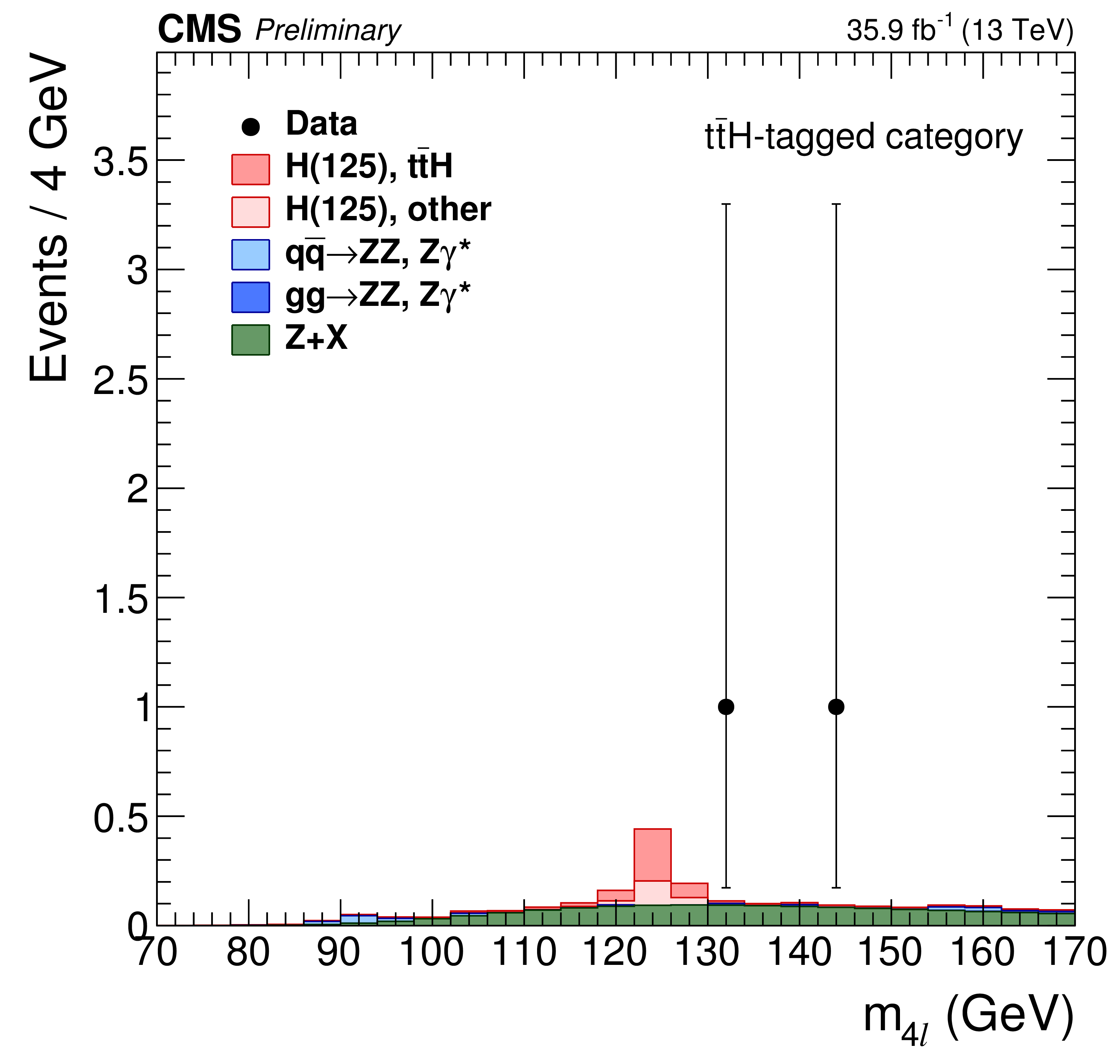
Figure 4-g:
Distribution of the four-lepton reconstructed mass in the ttH-tagged category. Points with error bars represent the data and stacked histograms represent expected distributions. The SM Higgs boson signal with $ {m_{\mathrm{ H } }}=$ 125 GeV, denoted as H(125), and the ZZ backgrounds are normalized to the SM expectation, the Z+X background to the estimation from data. The SM Higgs boson signal is separated into two components: the production mode which is targeted, and other production modes which is always dominated by the gluon fusion process. The order in pertubation theory used for the normalization of the irreducible backgrounds is described in Section 7.1. |
png pdf |
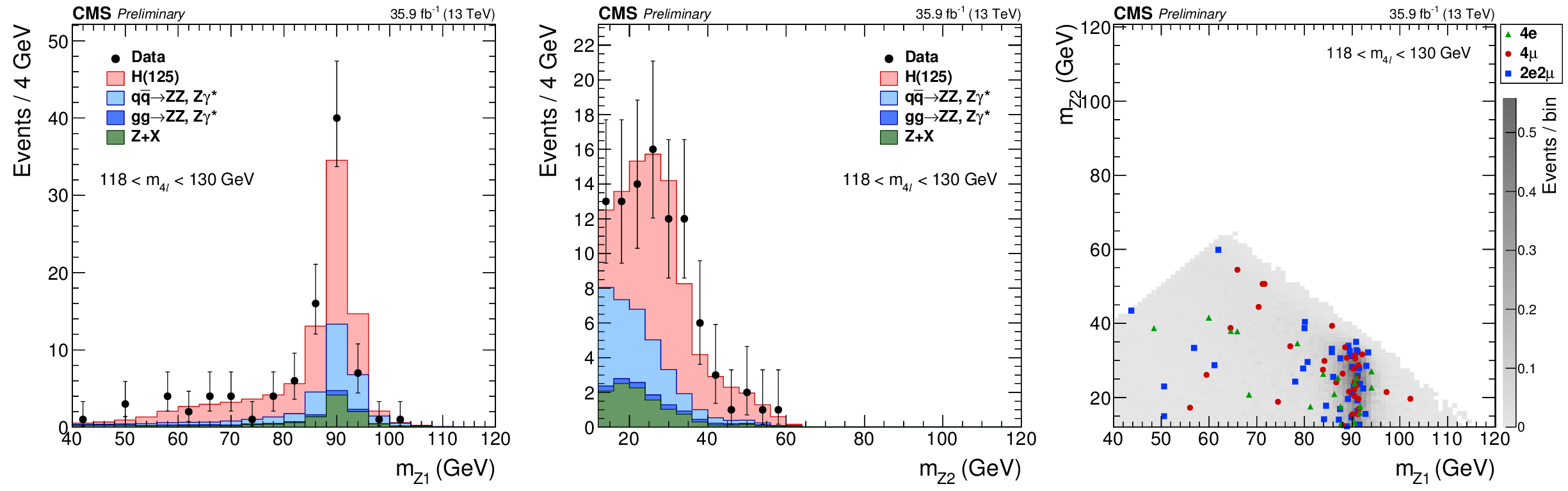
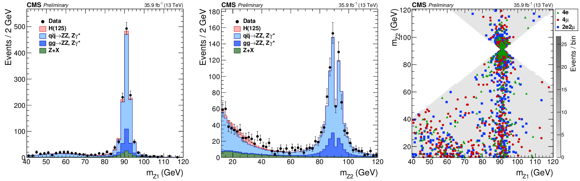
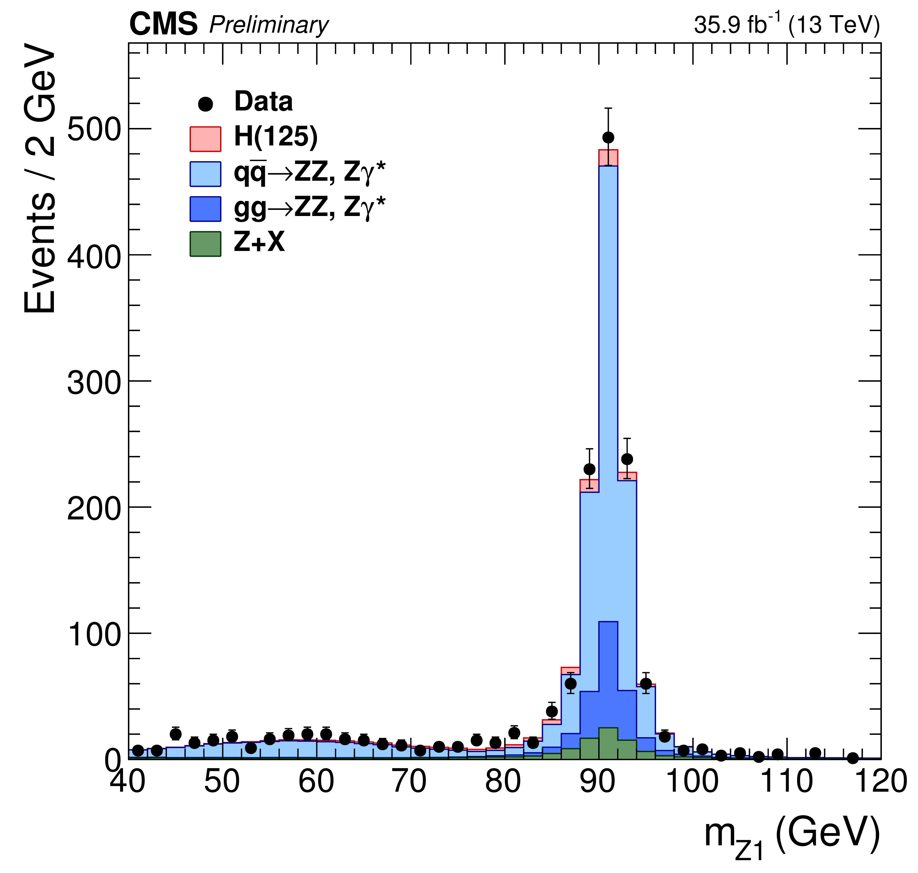
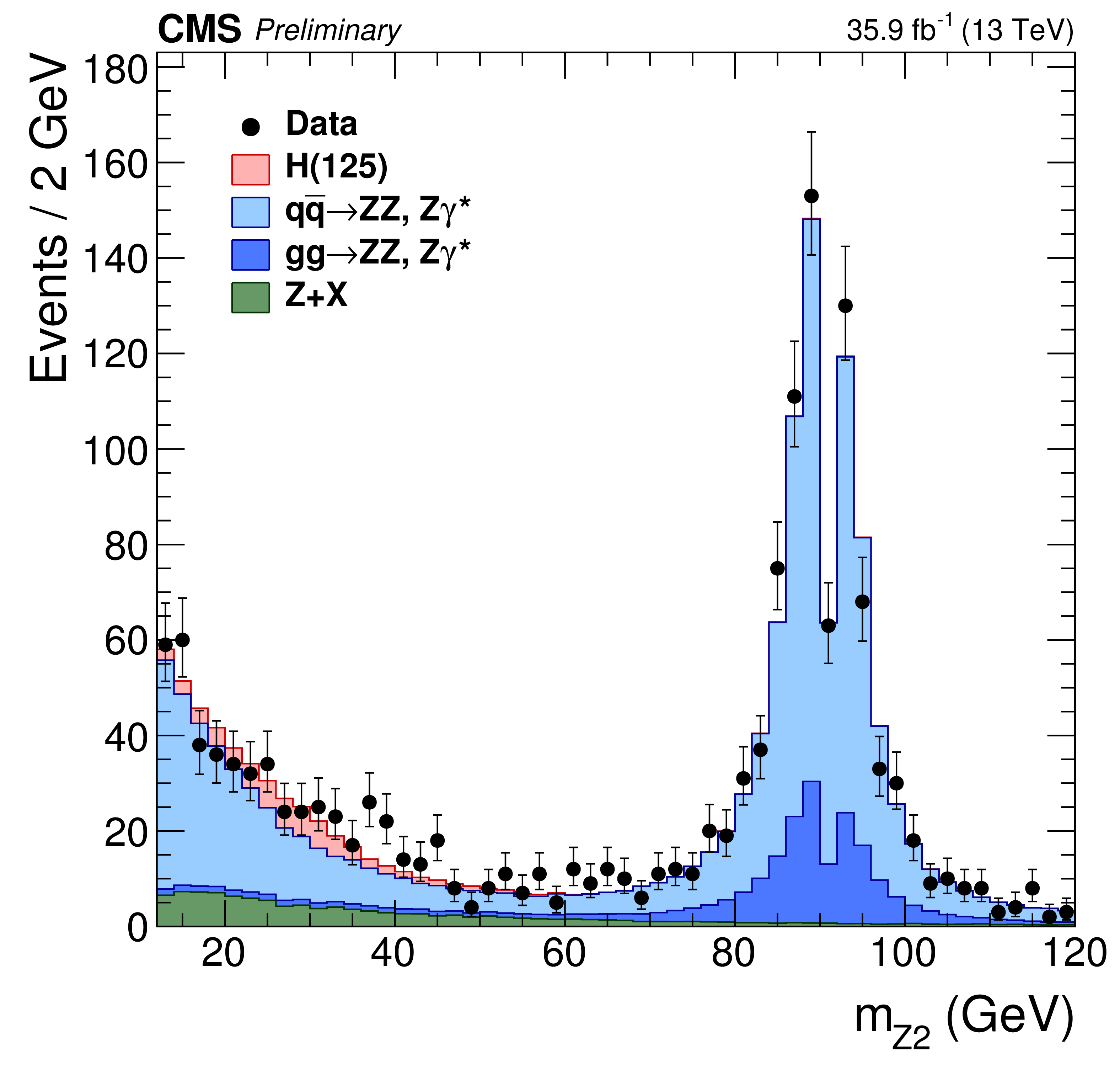
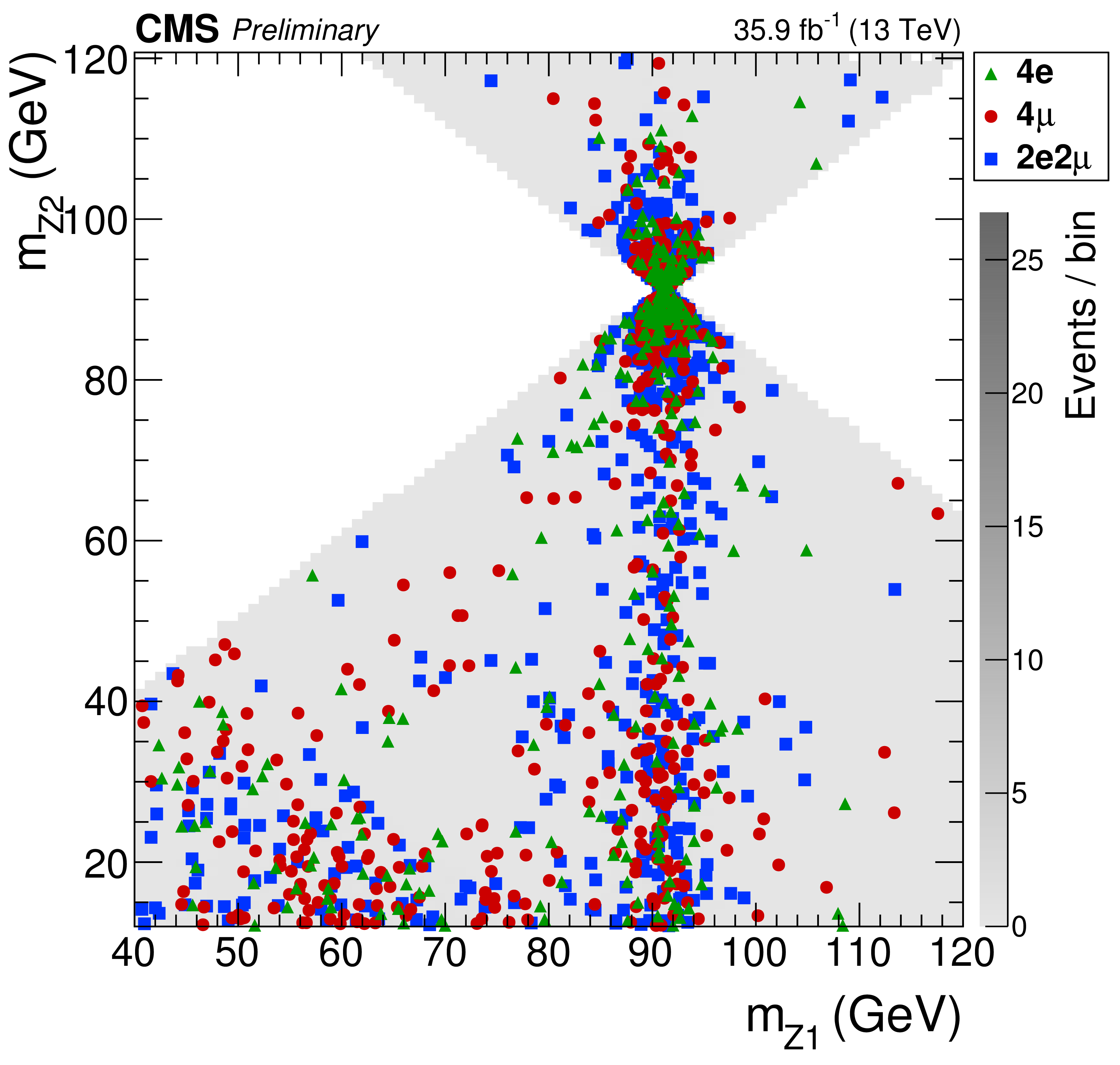
Figure 5:
Distribution of the $\mathrm{ Z } _1$ (left) and $\mathrm{ Z } _2$ (center) reconstructed invariant masses and correlation between the two (right) in the mass region 118 $ < {m_{4\ell }}< $ 130 GeV. The stacked histograms and the gray scale represent expected distributions, and points represent the data. The SM Higgs boson signal with $ {m_{\mathrm{ H } }}= $ 125 GeV, denoted as H(125), and the ZZ backgrounds are normalized to the SM expectation, the Z+X background to the estimation from data. The order in perturbation theory used for the normalization of the irreducible backgrounds is described in Section 7.1. |
png pdf |
Figure 5-a:
Correlation between $\mathrm{ Z } _1$ and $\mathrm{ Z } _2$ reconstructed invariant masses in the mass region 118 $ < {m_{4\ell }}< $ 130 GeV. The stacked histograms and the gray scale represent expected distributions, and points represent the data. The SM Higgs boson signal with $ {m_{\mathrm{ H } }}= $ 125 GeV, denoted as H(125), and the ZZ backgrounds are normalized to the SM expectation, the Z+X background to the estimation from data. The order in perturbation theory used for the normalization of the irreducible backgrounds is described in Section 7.1. |
png pdf |
Figure 5-b:
Distribution of the $\mathrm{ Z } _2$ reconstructed invariant mass in the mass region 118 $ < {m_{4\ell }}< $ 130 GeV. The stacked histograms and the gray scale represent expected distributions, and points represent the data. The SM Higgs boson signal with $ {m_{\mathrm{ H } }}= $ 125 GeV, denoted as H(125), and the ZZ backgrounds are normalized to the SM expectation, the Z+X background to the estimation from data. The order in perturbation theory used for the normalization of the irreducible backgrounds is described in Section 7.1. |
png pdf |
Figure 5-c:
Distribution of the $\mathrm{ Z } _1$ (left) and $\mathrm{ Z } _2$ (center) reconstructed invariant masses and correlation between the two (right) in the mass region 118 $ < {m_{4\ell }}< $ 130 GeV. The stacked histograms and the gray scale represent expected distributions, and points represent the data. The SM Higgs boson signal with $ {m_{\mathrm{ H } }}= $ 125 GeV, denoted as H(125), and the ZZ backgrounds are normalized to the SM expectation, the Z+X background to the estimation from data. The order in perturbation theory used for the normalization of the irreducible backgrounds is described in Section 7.1. |
png pdf |
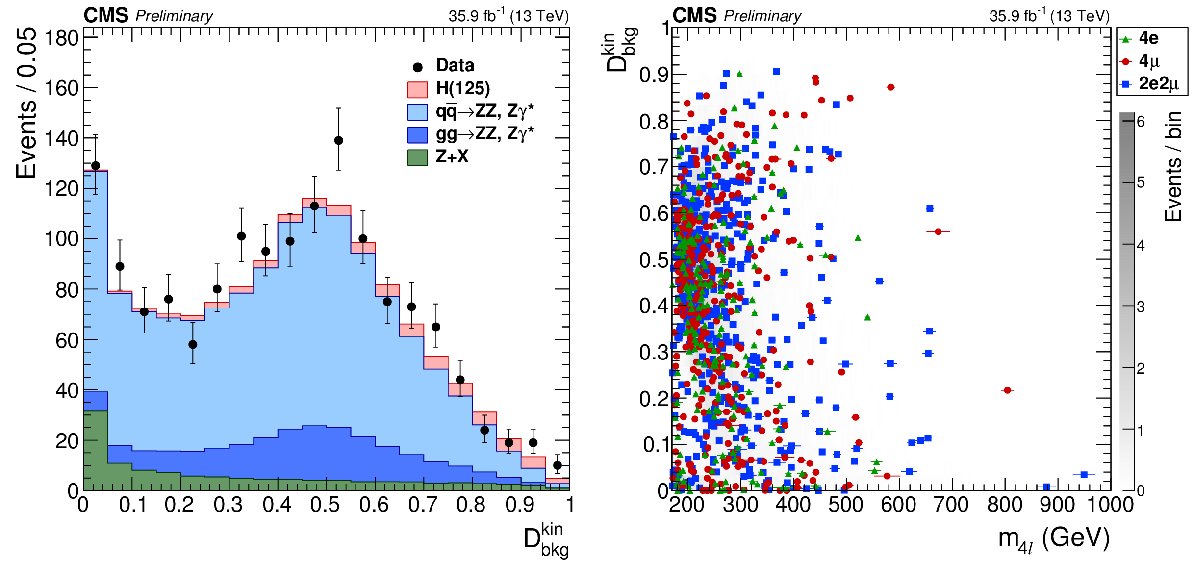
Figure 6:
Distribution of $ {{\cal D}^{\rm kin}_{\rm bkg}} $ versus $ {m_{4\ell }}$ in the mass region 100 $ < {m_{4\ell }}< $ 170 GeV. The gray scale represents the expected total number of ZZ background and SM Higgs boson signal events for $ {m_{\mathrm{ H } }}= $ 125 GeV. The points show the data and the horizontal bars represent the measured event-by-event mass uncertainties. Different marker styles are used to denote the categorization of the events. |
png pdf |
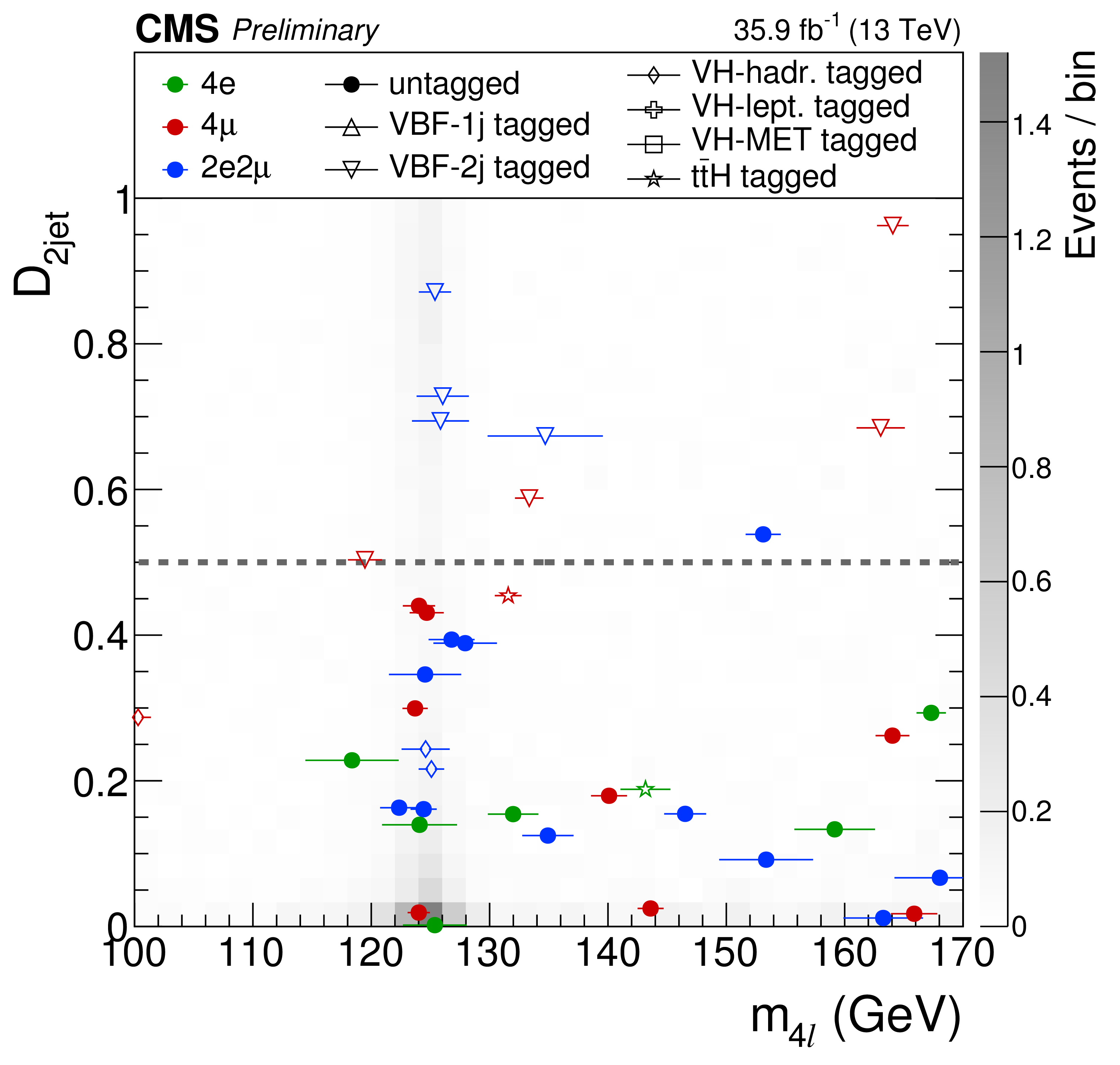
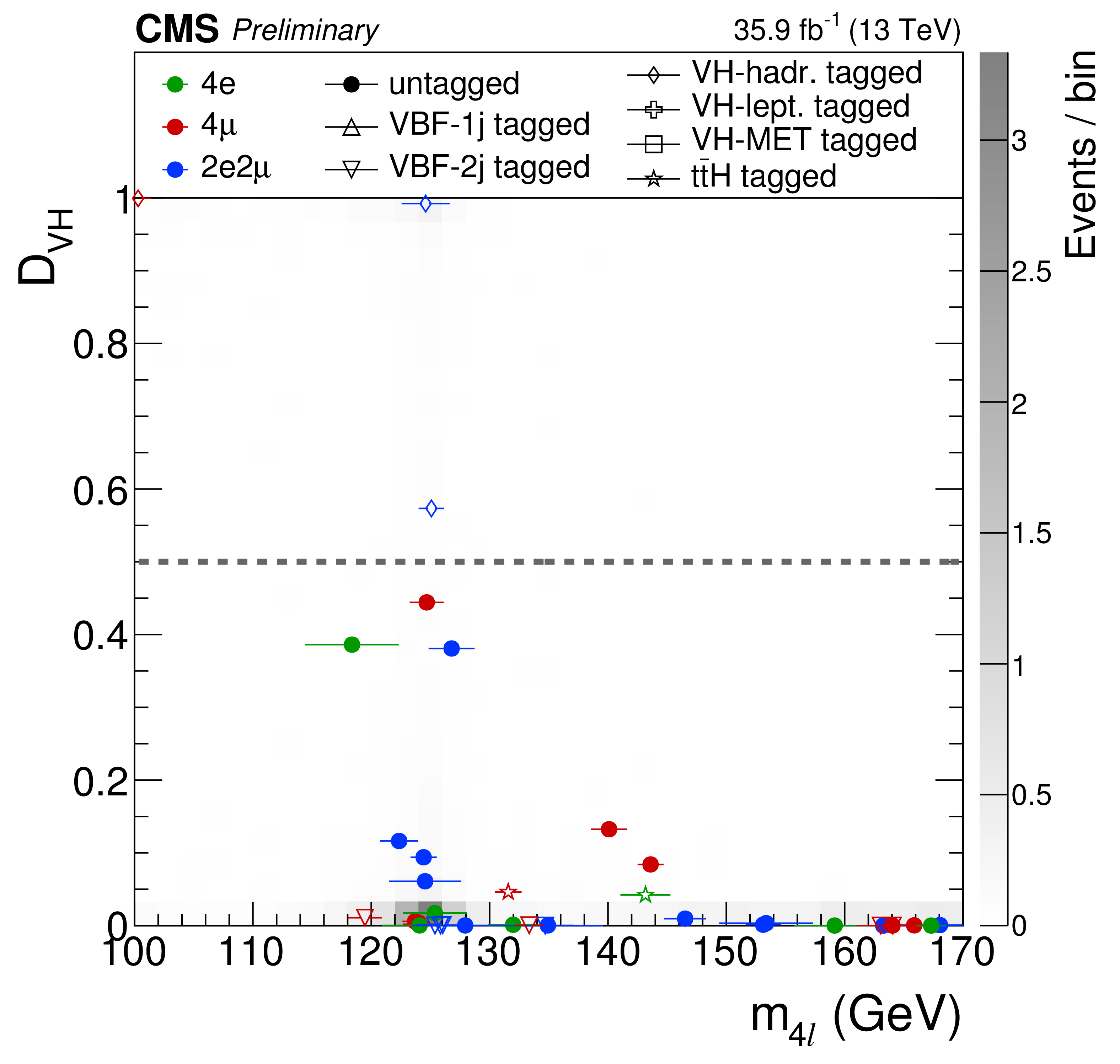
Figure 7:
Distribution of categorization discriminants in the mass region 118 $ < {m_{4\ell }} < $ 130 GeV. (Left) $ {{\mathcal D}_{\rm 2jet}} $ . (Middle) $ {{\mathcal D}_{\rm 1jet}} $ . (Right) ${{\mathcal D}_{\rm VH}} = max( {{\mathcal D}_{\rm {\mathrm{ W } \mathrm{ H } }}} $, ${{\mathcal D}_{\rm {\mathrm{ Z } \mathrm{ H } }}} $). Points with error bars represent the data and stacked histograms represent expected distributions. The SM Higgs boson signal with $ {m_{\mathrm{ H } }}= $ 125 GeV, denoted as H(125), and the ZZ backgrounds are normalized to the SM expectation, the Z+X background to the estimation from data. The vertical gray dashed lines denote the working points used in the event categorization. The SM Higgs boson signal is separated into two components: the production mode which is targeted by the specific discriminant, and other production modes which is always dominated by the gluon fusion process. The order in perturbation theory used for the normalization of the irreducible backgrounds is described in Section 7.1. |
png pdf |
Figure 7-a:
Distribution of the $ {{\mathcal D}_{\rm 2jet}} $ categorization discriminant in the mass region 118 $ < {m_{4\ell }} < $ 130 GeV. Points with error bars represent the data and stacked histograms represent expected distributions. The SM Higgs boson signal with $ {m_{\mathrm{ H } }}= $ 125 GeV, denoted as H(125), and the ZZ backgrounds are normalized to the SM expectation, the Z+X background to the estimation from data. The vertical gray dashed lines denote the working points used in the event categorization. The SM Higgs boson signal is separated into two components: the production mode which is targeted by the specific discriminant, and other production modes which is always dominated by the gluon fusion process. The order in perturbation theory used for the normalization of the irreducible backgrounds is described in Section 7.1. |
png pdf |
Figure 7-b:
Distribution of the $ {{\mathcal D}_{\rm 1jet}} $ categorization discriminant in the mass region 118 $ < {m_{4\ell }} < $ 130 GeV. Points with error bars represent the data and stacked histograms represent expected distributions. The SM Higgs boson signal with $ {m_{\mathrm{ H } }}= $ 125 GeV, denoted as H(125), and the ZZ backgrounds are normalized to the SM expectation, the Z+X background to the estimation from data. The vertical gray dashed lines denote the working points used in the event categorization. The SM Higgs boson signal is separated into two components: the production mode which is targeted by the specific discriminant, and other production modes which is always dominated by the gluon fusion process. The order in perturbation theory used for the normalization of the irreducible backgrounds is described in Section 7.1. |
png pdf |
Figure 7-c:
Distribution of the ${{\mathcal D}_{\rm VH}} = max( {{\mathcal D}_{\rm {\mathrm{ W } \mathrm{ H } }}} $, ${{\mathcal D}_{\rm {\mathrm{ Z } \mathrm{ H } }}} $) categorization discriminant in the mass region 118 $ < {m_{4\ell }} < $ 130 GeV. Points with error bars represent the data and stacked histograms represent expected distributions. The SM Higgs boson signal with $ {m_{\mathrm{ H } }}= $ 125 GeV, denoted as H(125), and the ZZ backgrounds are normalized to the SM expectation, the Z+X background to the estimation from data. The vertical gray dashed lines denote the working points used in the event categorization. The SM Higgs boson signal is separated into two components: the production mode which is targeted by the specific discriminant, and other production modes which is always dominated by the gluon fusion process. The order in perturbation theory used for the normalization of the irreducible backgrounds is described in Section 7.1. |
png pdf |
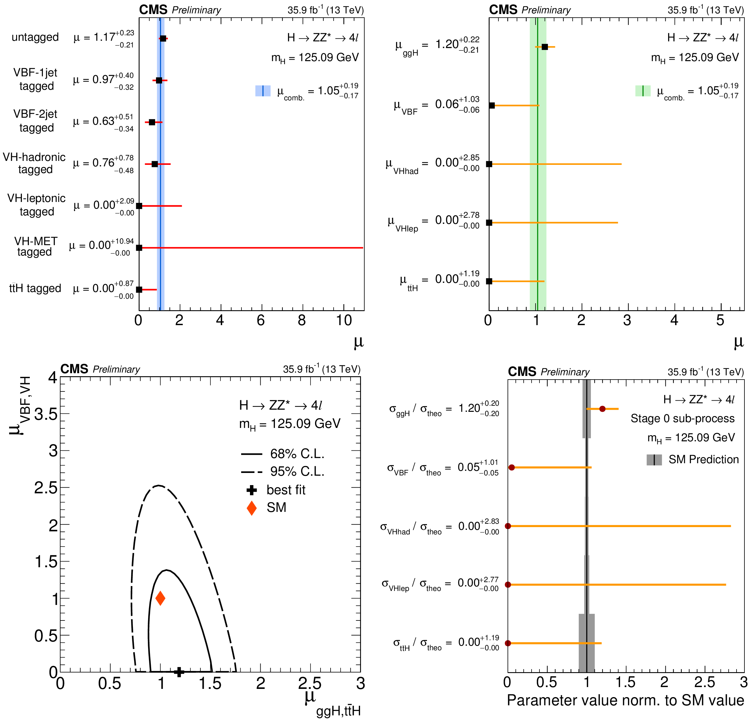
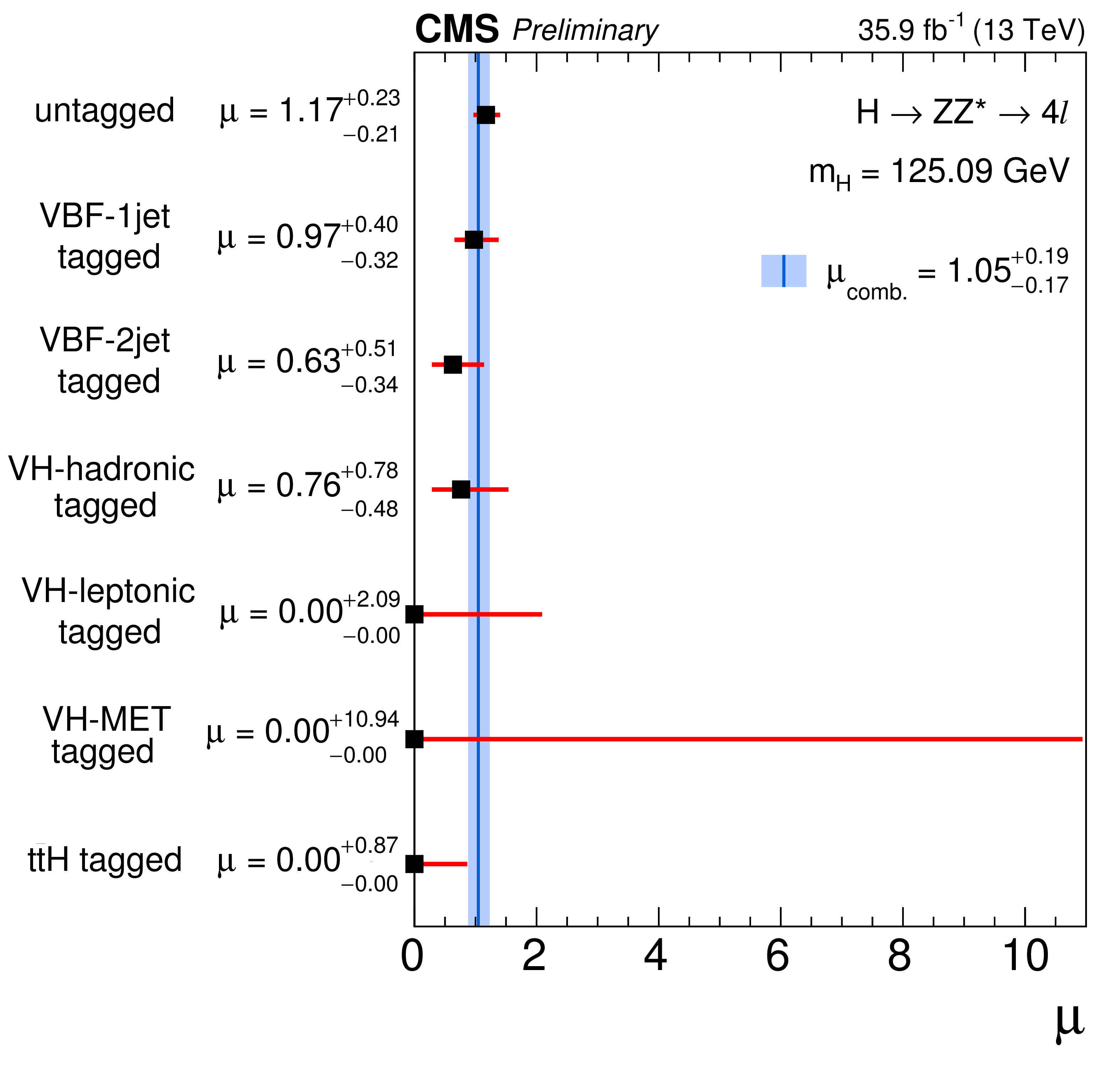
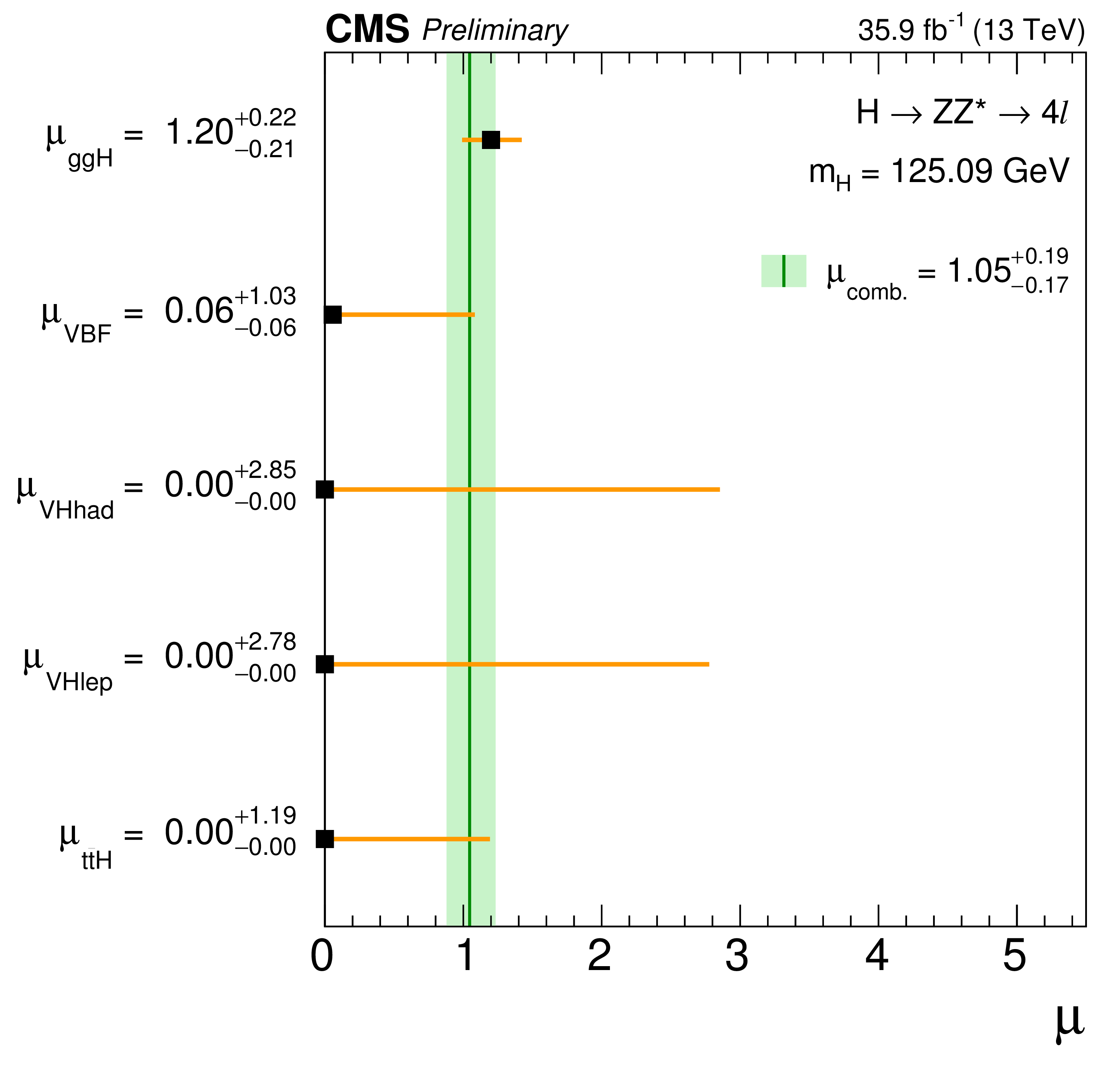
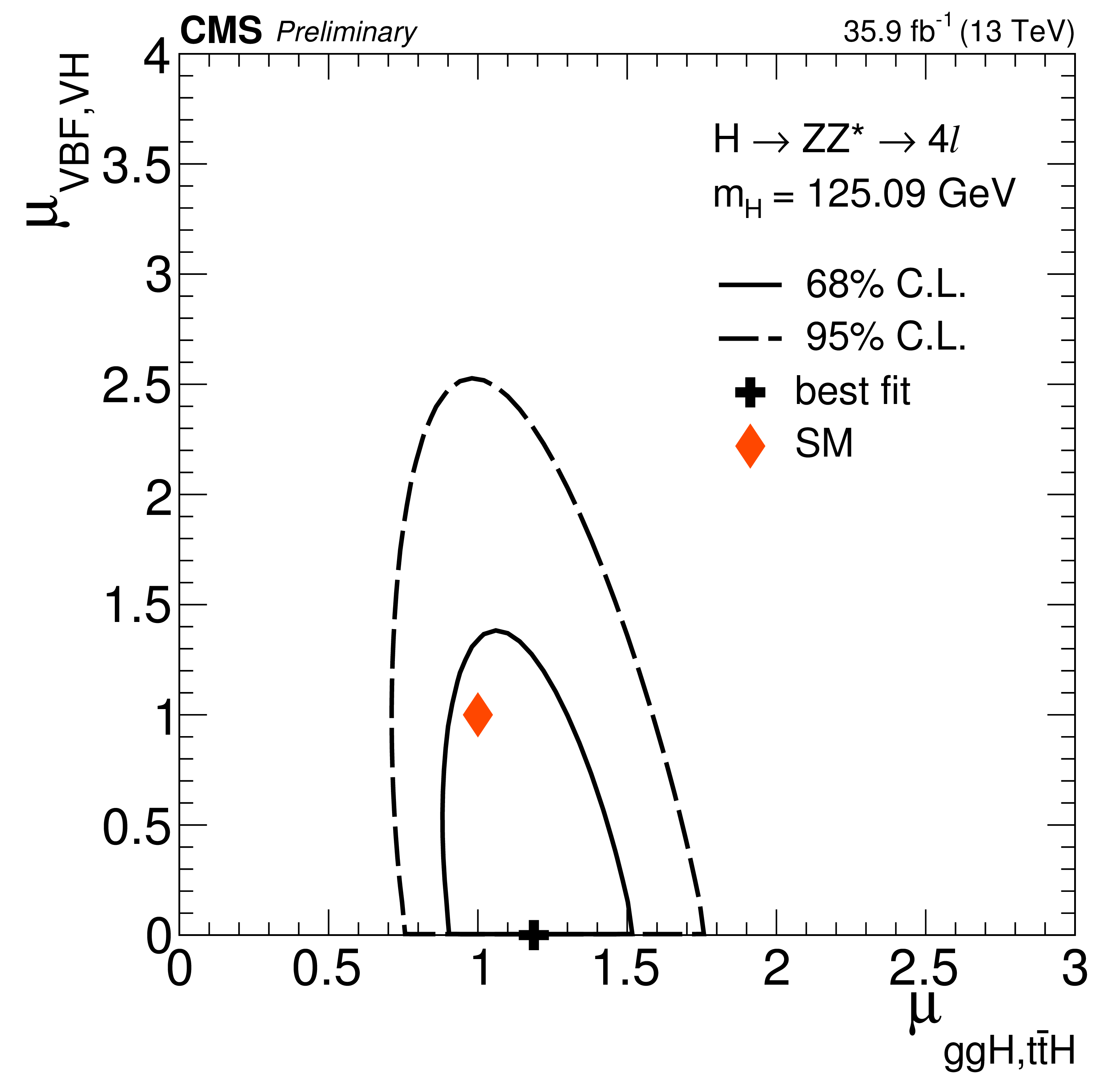
Figure 8:
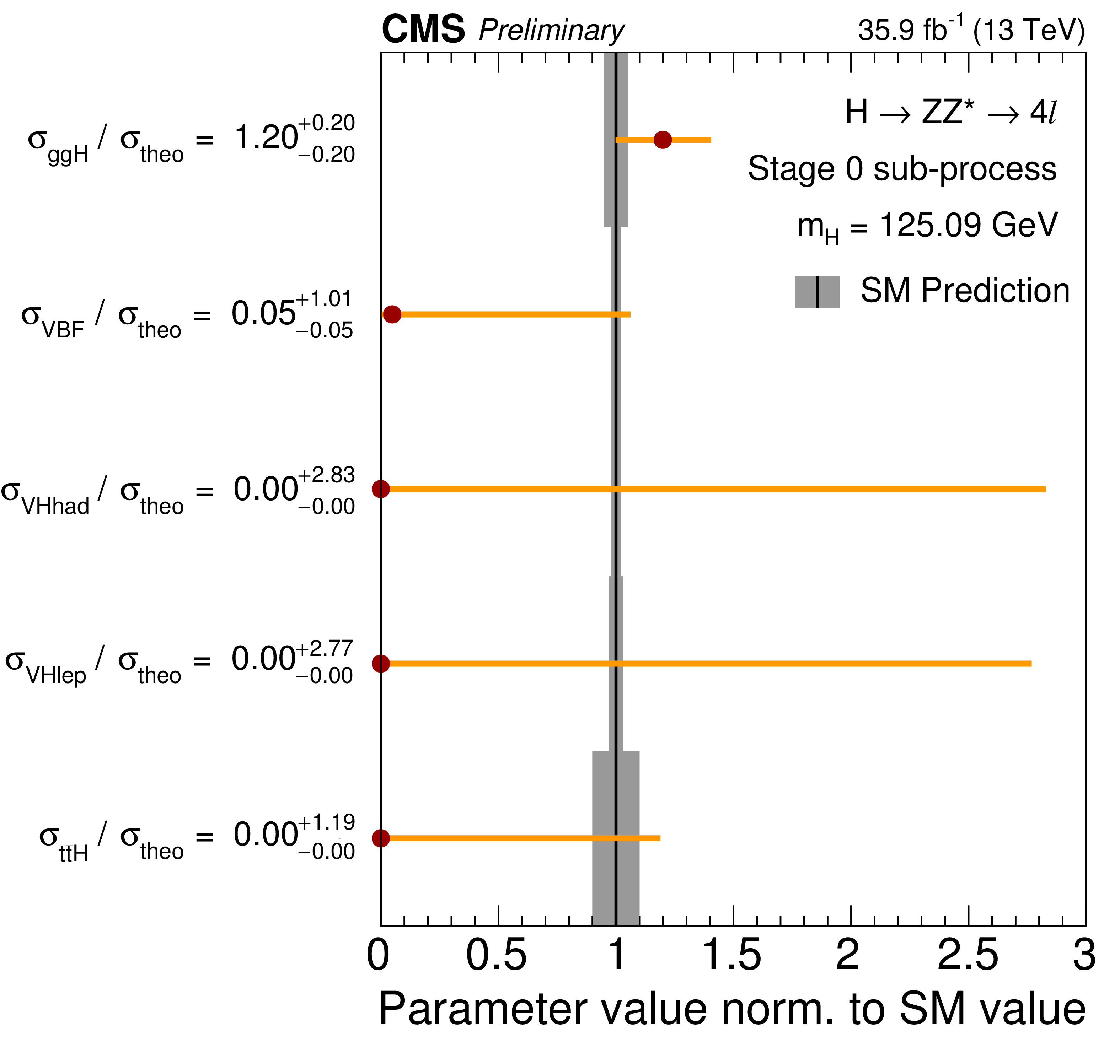
(Top left) Observed values of the signal strength $\mu =\sigma /\sigma _{SM}$ for the seven event categories, compared to the combined $\mu $ shown as a vertical line. The horizontal bars and the filled band indicate the $\pm $1$\sigma $ uncertainties. (Top right) Results of likelihood scans for the signal-strength modifiers corresponding to the main SM Higgs boson production modes, compared to the combined $\mu $ shown as a vertical line. The horizontal bars and the filled band indicate the $\pm $1$\sigma $ uncertainties. The uncertainties include both statistical and systematic sources. (Bottom left) Result of the 2D likelihood scan for the $ {\mu _{\mathrm{g} \mathrm{g} \mathrm{ H } , {\mathrm{ t } {}\mathrm{ \bar{t} } } \mathrm{ H } }} $ and $ {\mu _{\mathrm {VBF},\mathrm {V\mathrm{ H } }}} $ signal-strength modifiers. The solid and dashed contours show the 68% and 95% CL regions, respectively. The cross indicates the best-fit values, and the diamond represents the expected values for the SM Higgs boson. (Bottom right) Results of the fit for simplified template cross sections for the stage 0 sub-processes, normalized to the SM prediction. |
png pdf |
Figure 8-a:
Observed values of the signal strength $\mu =\sigma /\sigma _{SM}$ for the seven event categories, compared to the combined $\mu $ shown as a vertical line. The horizontal bars and the filled band indicate the $\pm $1$\sigma $ uncertainties. |
png pdf |
Figure 8-b:
Results of likelihood scans for the signal-strength modifiers corresponding to the main SM Higgs boson production modes, compared to the combined $\mu $ shown as a vertical line. The horizontal bars and the filled band indicate the $\pm $1$\sigma $ uncertainties. The uncertainties include both statistical and systematic sources. |
png pdf |
Figure 8-c:
Result of the 2D likelihood scan for the $ {\mu _{\mathrm{g} \mathrm{g} \mathrm{ H } , {\mathrm{ t } {}\mathrm{ \bar{t} } } \mathrm{ H } }} $ and $ {\mu _{\mathrm {VBF},\mathrm {V\mathrm{ H } }}} $ signal-strength modifiers. The solid and dashed contours show the 68% and 95% CL regions, respectively. The cross indicates the best-fit values, and the diamond represents the expected values for the SM Higgs boson. |
png pdf |
Figure 8-d:
Results of the fit for simplified template cross sections for the stage 0 sub-processes, normalized to the SM prediction. |
png pdf |
Figure 9:
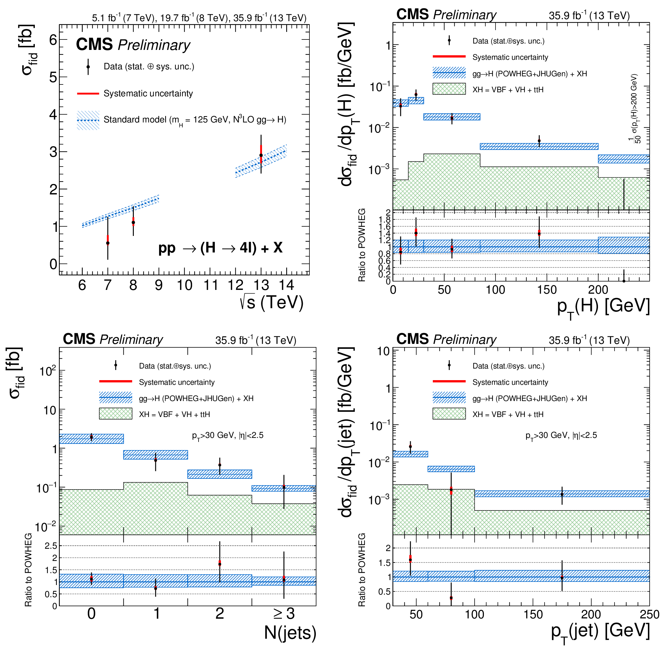
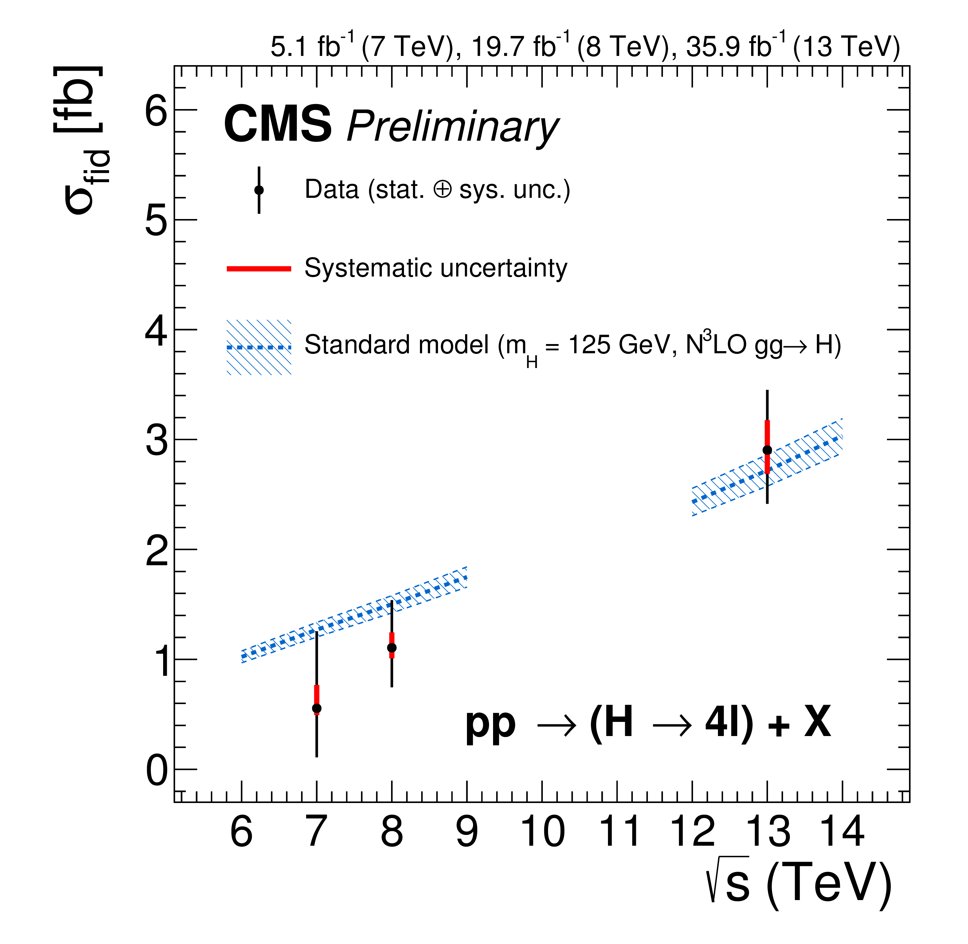
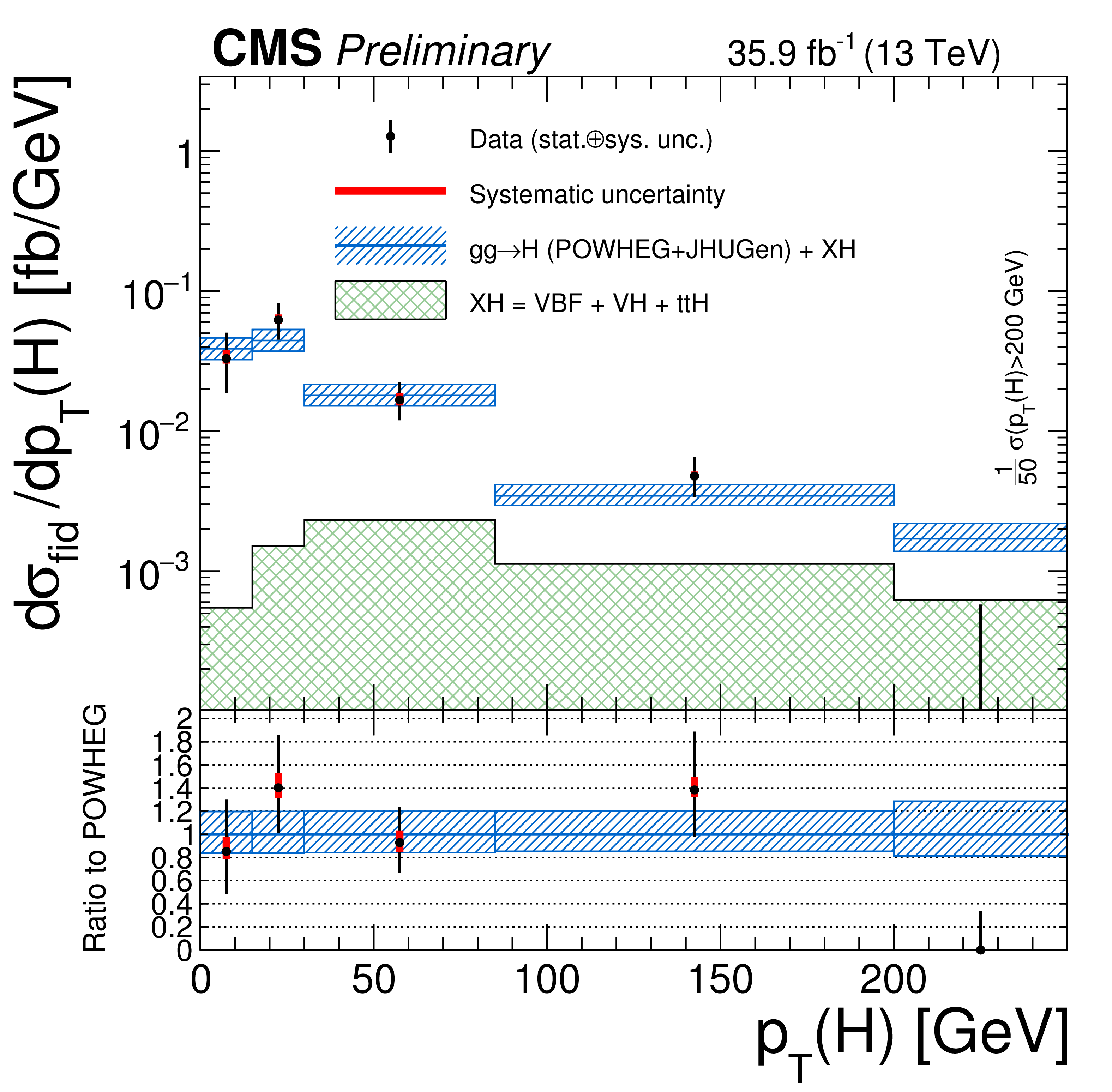
The measured fiducial cross section as a function of $\sqrt {s}$ (top left). The acceptance is calculated using POWHEG at $\sqrt {s}= $ 13 TeV and HRes [50,52] at $\sqrt {s}= $ 7 and 8 TeV and the total gluon fusion cross section and uncertainty are taken from Ref. [24]. The fiducial volume for $\sqrt {s}= $ 6-9 TeV uses the lepton isolation definition from Ref. [18], while for $\sqrt {s} = $ 12-14 TeV the definition described in the text is used. The results of the differential cross section measurement for $ {p_{\mathrm {T}}} ({\rm H})$ (top right), N(jets) (bottom left) and $ {p_{\mathrm {T}}} ({\rm jet})$ (bottom right). The acceptance and theoretical uncertainties in the differential bins are are calculated using POWHEG . The sub-dominant component of the the signal (VBF $+$ VH $+ {\mathrm{ t } \bar{\mathrm{ t } }\mathrm{ H } }$) is denoted as XH. |
png pdf |
Figure 9-a:
The measured fiducial cross section as a function of $\sqrt {s}$ (top left). The acceptance is calculated using POWHEG at $\sqrt {s}= $ 13 TeV and HRes [50,52] at $\sqrt {s}= $ 7 and 8 TeV and the total gluon fusion cross section and uncertainty are taken from Ref. [24]. The fiducial volume for $\sqrt {s}= $ 6-9 TeV uses the lepton isolation definition from Ref. [18], while for $\sqrt {s} = $ 12-14 TeV the definition described in the text is used. |
png pdf |
Figure 9-b:
The results of the differential cross section measurement for $ {p_{\mathrm {T}}} ({\rm H})$. The acceptance and theoretical uncertainties in the differential bins are are calculated using POWHEG . The sub-dominant component of the the signal (VBF $+$ VH $+ {\mathrm{ t } \bar{\mathrm{ t } }\mathrm{ H } }$) is denoted as XH. |
png pdf |
Figure 9-c:
The results of the differential cross section measurement for N(jets). The acceptance and theoretical uncertainties in the differential bins are are calculated using POWHEG . The sub-dominant component of the the signal (VBF $+$ VH $+ {\mathrm{ t } \bar{\mathrm{ t } }\mathrm{ H } }$) is denoted as XH. |
png pdf |
Figure 9-d:
The results of the differential cross section measurement for $ {p_{\mathrm {T}}} ({\rm jet})$. The acceptance and theoretical uncertainties in the differential bins are are calculated using POWHEG . The sub-dominant component of the the signal (VBF $+$ VH $+ {\mathrm{ t } \bar{\mathrm{ t } }\mathrm{ H } }$) is denoted as XH. |
png pdf |
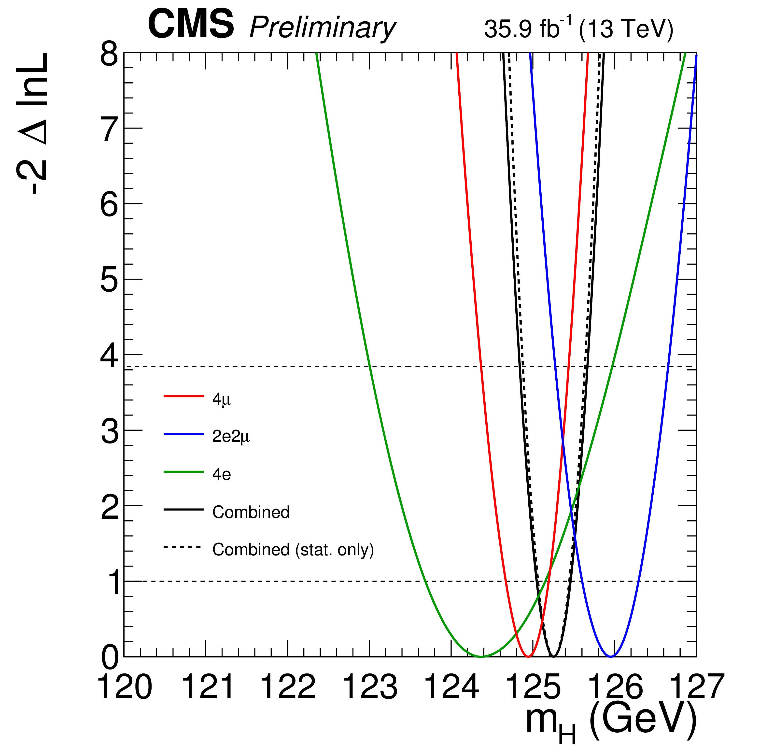
Figure 10:
Left: 1D likelihood scan as a function of mass for the 1D, 2D, and 3D measurement. Right: 1D likelihood scan as a function of mass for the different final states and the combination of all final states for the 3D measurement. The likelihood scans are shown for the mass measurement using the refitted mass distribution with $m(\mathrm{ Z } _1)$ constraint. Solid lines represents the scan with full uncertainties included, dashed lines statistical uncertainty only. |
png pdf |
Figure 10-a:
1D likelihood scan as a function of mass for the 1D, 2D, and 3D measurement. The likelihood scan is shown for the mass measurement using the refitted mass distribution with $m(\mathrm{ Z } _1)$ constraint. Solid lines represents the scan with full uncertainties included, dashed lines statistical uncertainty only. |
png pdf |
Figure 10-b:
1D likelihood scan as a function of mass for the different final states and the combination of all final states for the 3D measurement. The likelihood scan is shown for the mass measurement using the refitted mass distribution with $m(\mathrm{ Z } _1)$ constraint. Solid lines represents the scan with full uncertainties included, dashed lines statistical uncertainty only. |
png pdf |
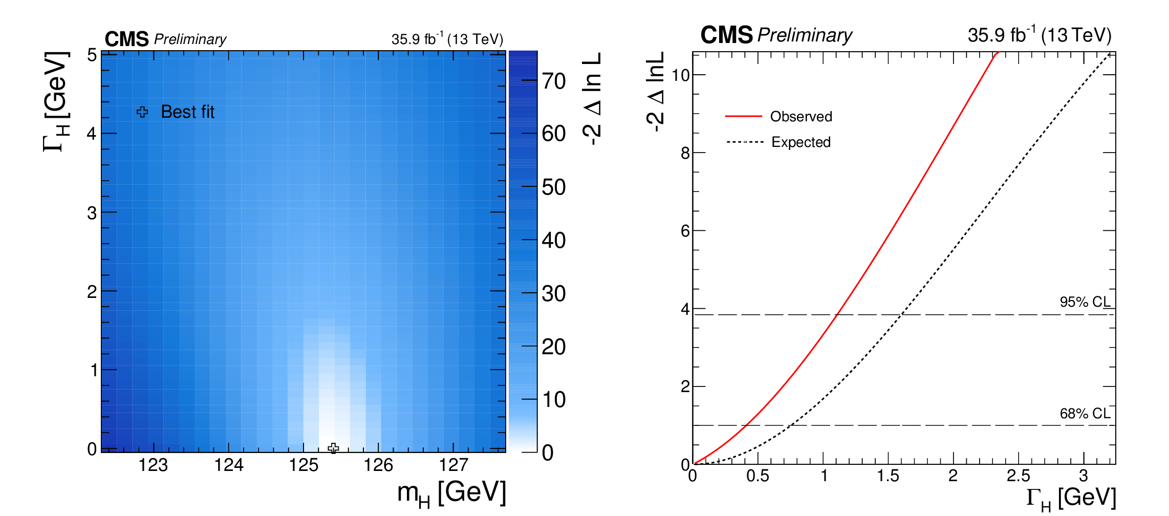
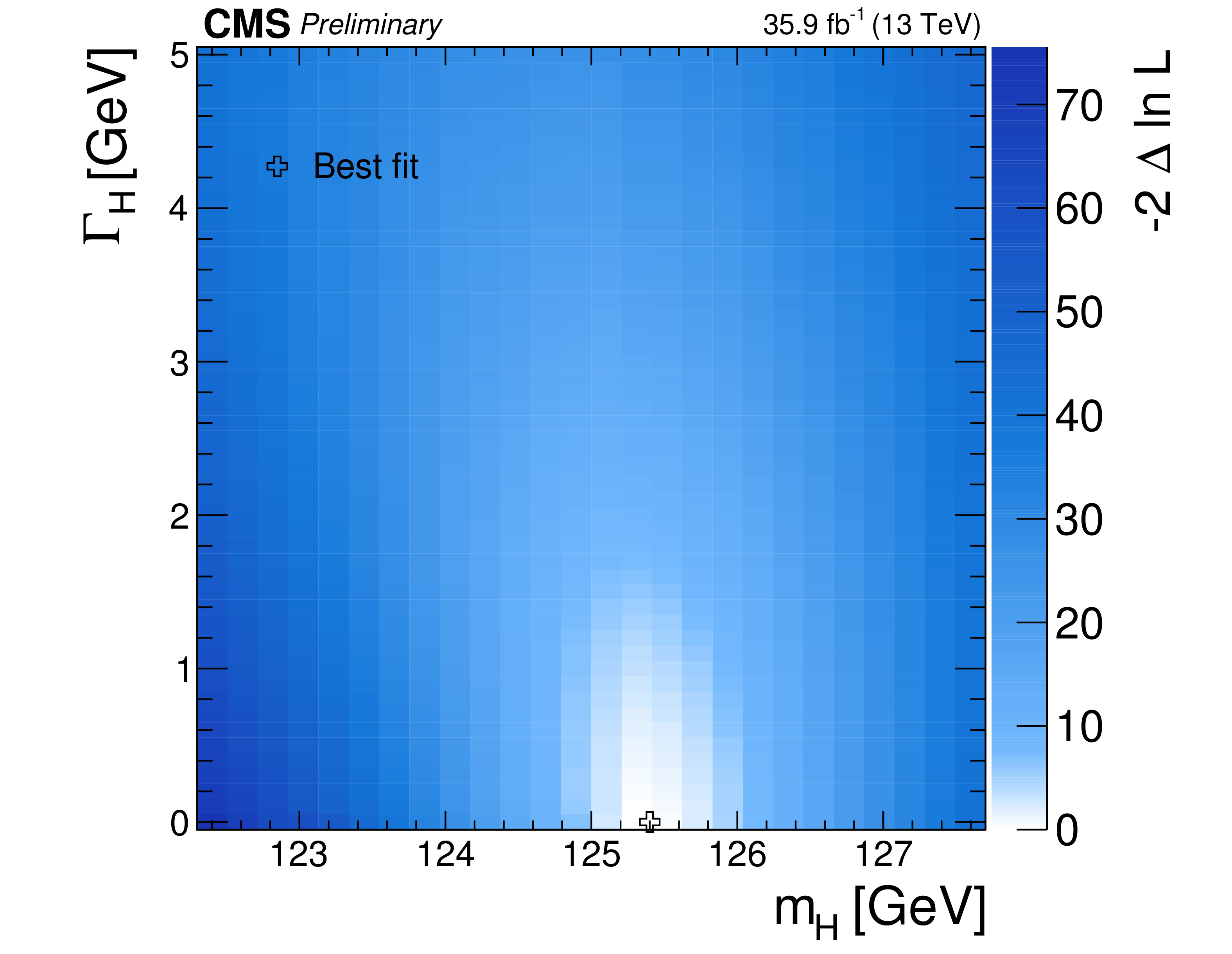
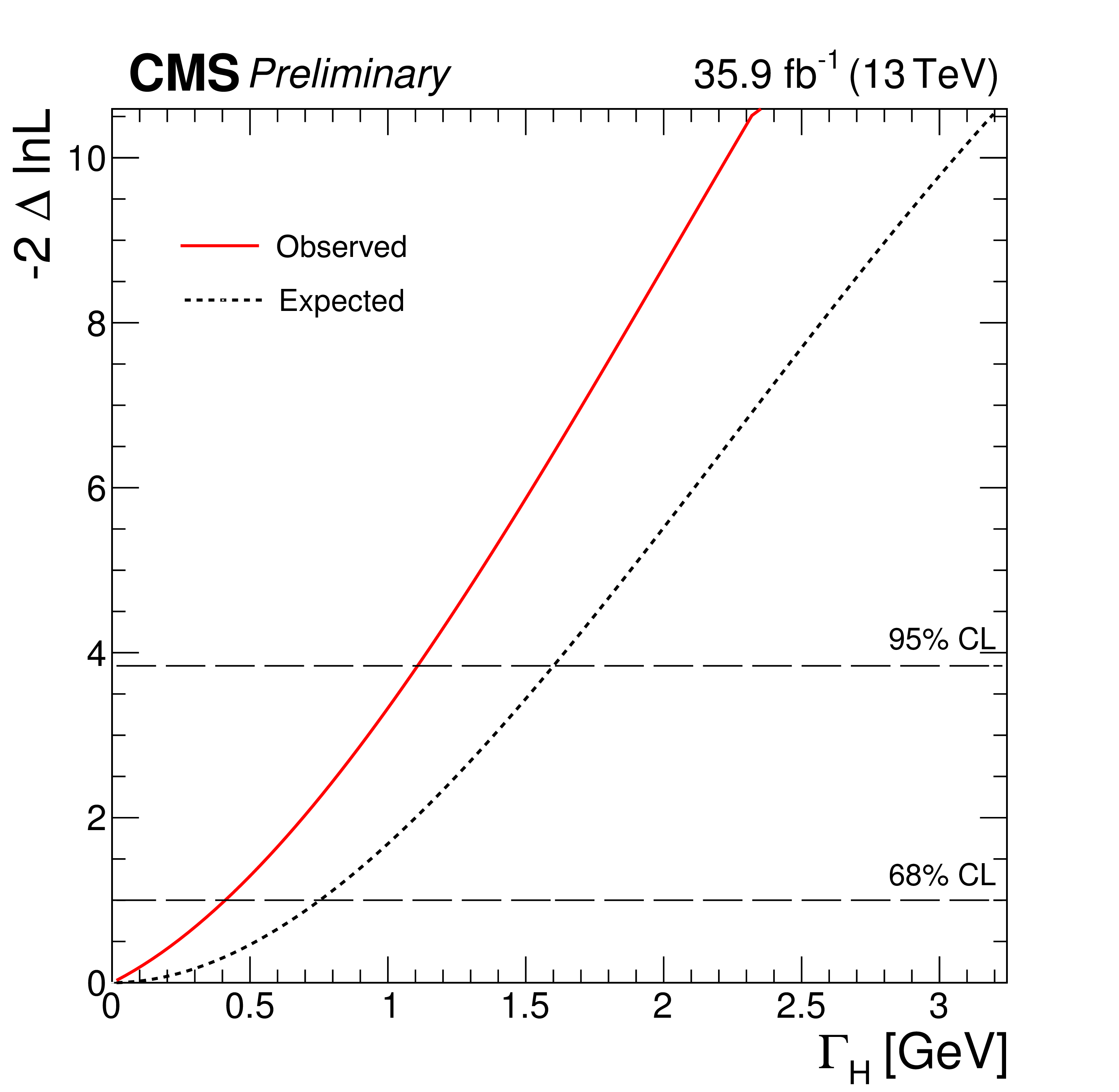
Figure 11:
(Left) Observed likelihood scan of $m_{\rm H}$ and $\Gamma _{\rm H}$ using the signal range 105 $ < m_{4\ell } < $ 140 GeV. (Right) Observed and expected likelihood scan of $\Gamma _{\rm H}$ using the signal range 105 $ < m_{4\ell } < $ 140 GeV, with $m_{\rm H}$ floated. |
png pdf |
Figure 11-a:
Observed likelihood scan of $m_{\rm H}$ and $\Gamma _{\rm H}$ using the signal range 105 $ < m_{4\ell } < $ 140 GeV. |
png pdf |
Figure 11-b:
Observed and expected likelihood scan of $\Gamma _{\rm H}$ using the signal range 105 $ < m_{4\ell } < $ 140 GeV, with $m_{\rm H}$ floated. |
| Tables | |
png pdf |
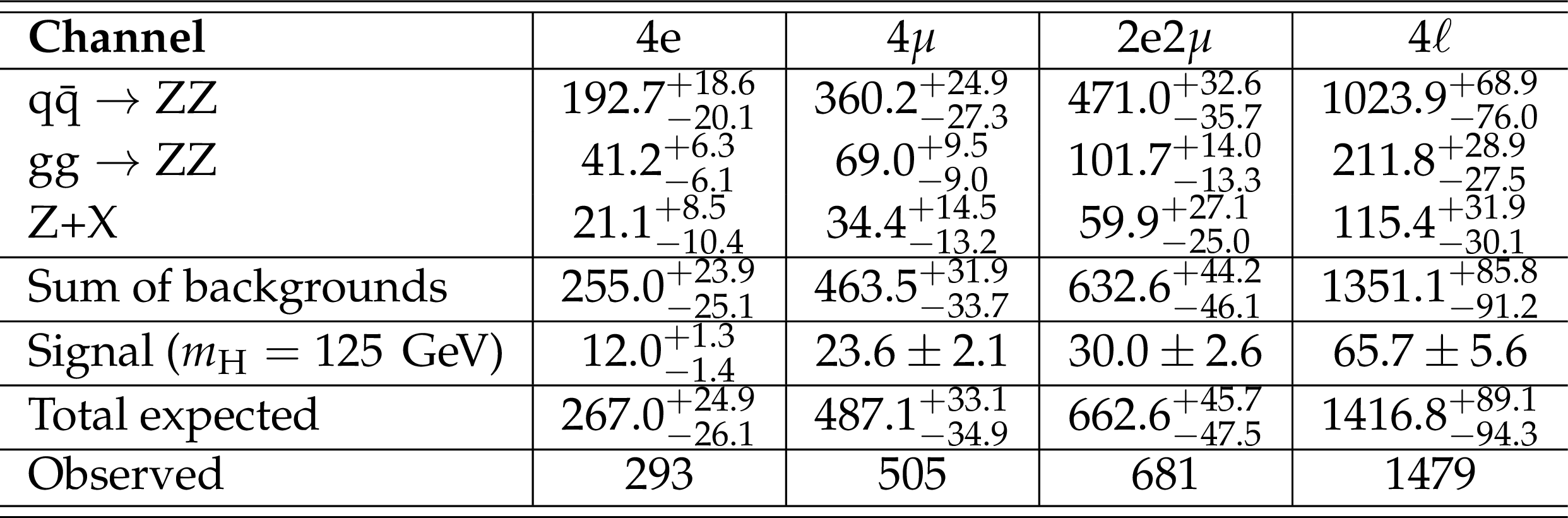
Table 1:
The number of expected background and signal events and number observed candidates after full analysis selection, for each final state, for the full mass range $ {m_{4\ell }}> $ 70 GeV, for an integrated luminosity of 35.9fb$^{-1}$. Signal and ZZ backgrounds are estimated from Monte Carlo simulation, Z+X is estimated from data. |
png pdf |
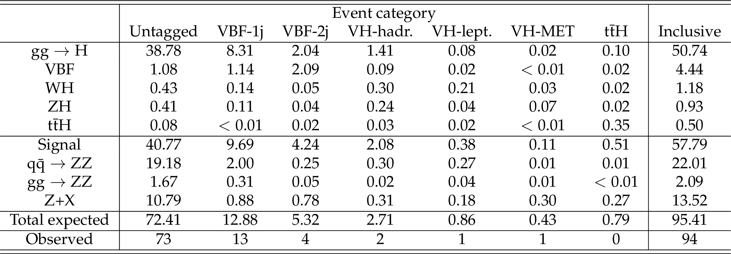
Table 2:
The number of expected background and signal events and number of observed candidates after full analysis selection, for each event category, for the mass range 118 $ < {m_{4\ell }}< $ 130 GeV, for an integrated luminosity of 35.9fb$^{-1}$. The yields are given for the different production modes. Signal and ZZ backgrounds are estimated from Monte Carlo simulation, Z+X is estimated from data. |

png pdf |
Table 3:
Expected and observed signal-strength modifiers. |
png pdf |
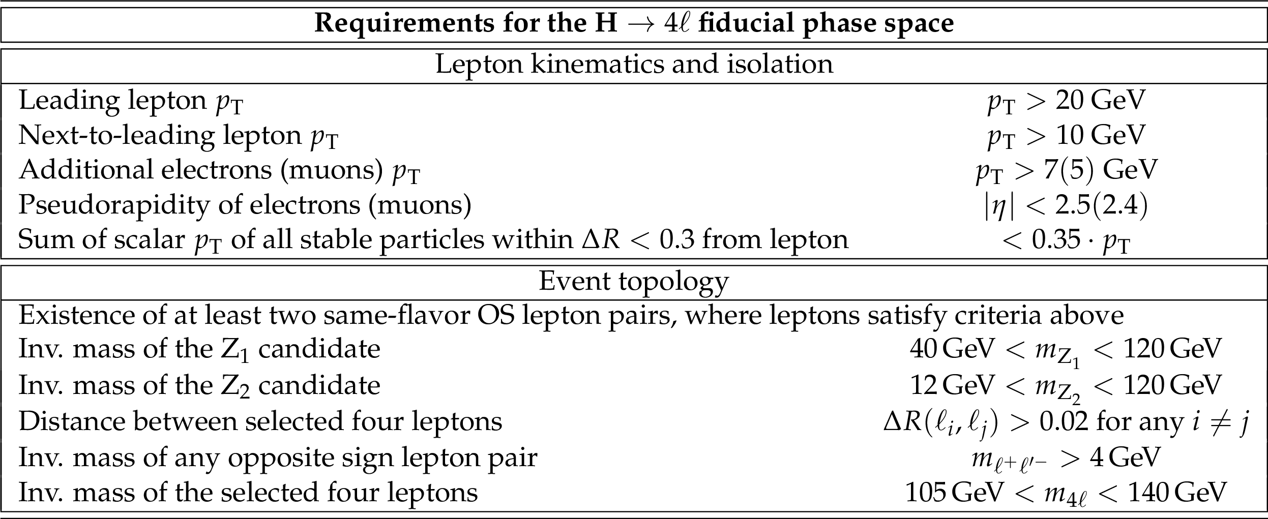
Table 4:
Summary of requirements and selections used in the definition of the fiducial phase space for the $ {\mathrm{ H } \to 4\ell }$ cross section measurements. |
png pdf |
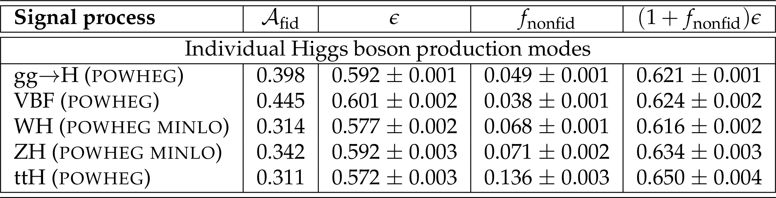
Table 5:
Summary of different SM signal models. For all production modes the values given are for $m_{\rm H}=$ 125 GeV. The uncertainties listed are statistical uncertainties only, and the statistical uncertainty on the acceptance is $\sim $0.001. |
png pdf |
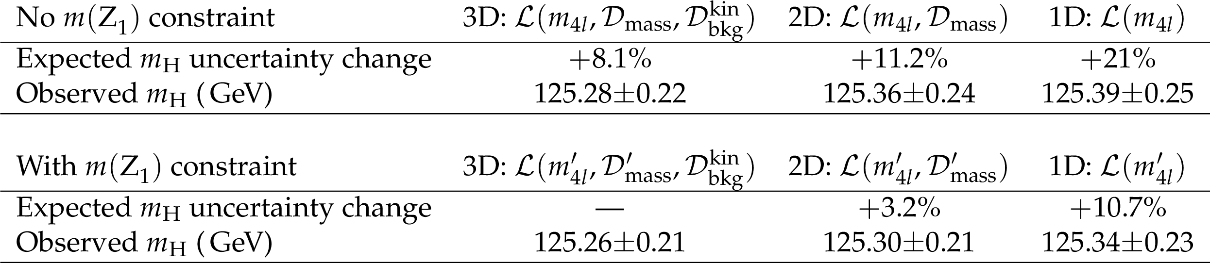
Table 6:
Best fit values for the mass of the Higgs boson measured in the $4\ell $, $\ell =\mathrm{ e } ,\mu $ final states, with 1D, 2D and 3D fit, respectively, as described in the text. All mass values are given in GeV. The uncertainties are the total statistical plus systematic uncertainty. The expected $ {m_{\mathrm{ H } }}$ uncertainty change shows the change in expected precision on the measurement for the different fit scenarios, relative to 3D ${\cal L}(m'_{4l},\mathrm {{\cal D}'_{\rm mass}} , {{\cal D}^{\rm kin}_{\rm bkg}} )$. |
png pdf |
Table 7:
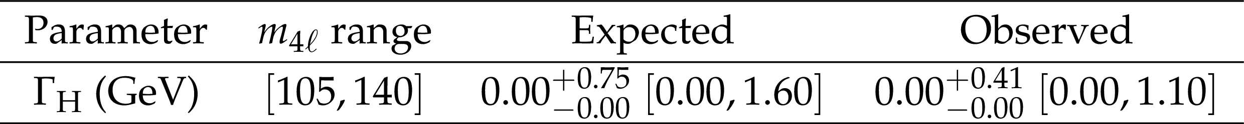
Summary of allowed 68%CL (central values with uncertainties) and 95%CL (ranges in square brackets) intervals on the width $\Gamma _{\rm H}$ of the Higgs boson. The expected results are quoted for the SM signal production cross section ($\mu _{\rm VBF,VH}=\mu _{\rm ggH,t\bar{t}H}= $ 1) and the values of $m_{\rm H}= $ 125 GeV and $\Gamma _{\rm H}= $ 0.0041 GeV. |
| Summary |
| Several measurements of Higgs boson production in the four-lepton final state at $ \sqrt{s} = $ 13 TeV have been presented, using data samples corresponding to an integrated luminosity of 35.9 fb$^{-1}$. The measured signal strength modifier is $\mu =$ 1.05$^{+0.19}_{-0.17}$ = 1.05$^{+0.15}_{-0.14}$ (stat.) $^{+0.11}_{-0.09}$ (sys.), and the measured signal strength modifiers associated with fermions and vector bosons are ${\mu_{\mathrm{gg}\mathrm{ H },\,\mathrm{ t \bar{t} }\mathrm{ H }}} =$ 1.20$^{+0.35}_{-0.31}$ and ${\mu_{\mathrm{VBF},\mathrm{V\mathrm{ H }}}} =$ 0.00$^{+1.37}_{-0.00}$, respectively. The fiducial cross section at $ \sqrt{s} = $ 13 TeV for this boson is measured to be 2.90$^{+0.48}_{-0.44} $ (stat.) $^{+0.27}_{-0.22}$ (sys.) fb. The mass is measured to be $m_{{\rm H}}=$ 125.26 $\pm$ 0.20 (stat.) $\pm$ 0.08 (sys.) GeV and the width is constrained to be $\Gamma_{{\rm H}}< $ 1.10 GeV at 95% CL. All results are consistent, within their uncertainties, with the expectations for the SM Higgs boson. |
| Additional Figures | |
png pdf |
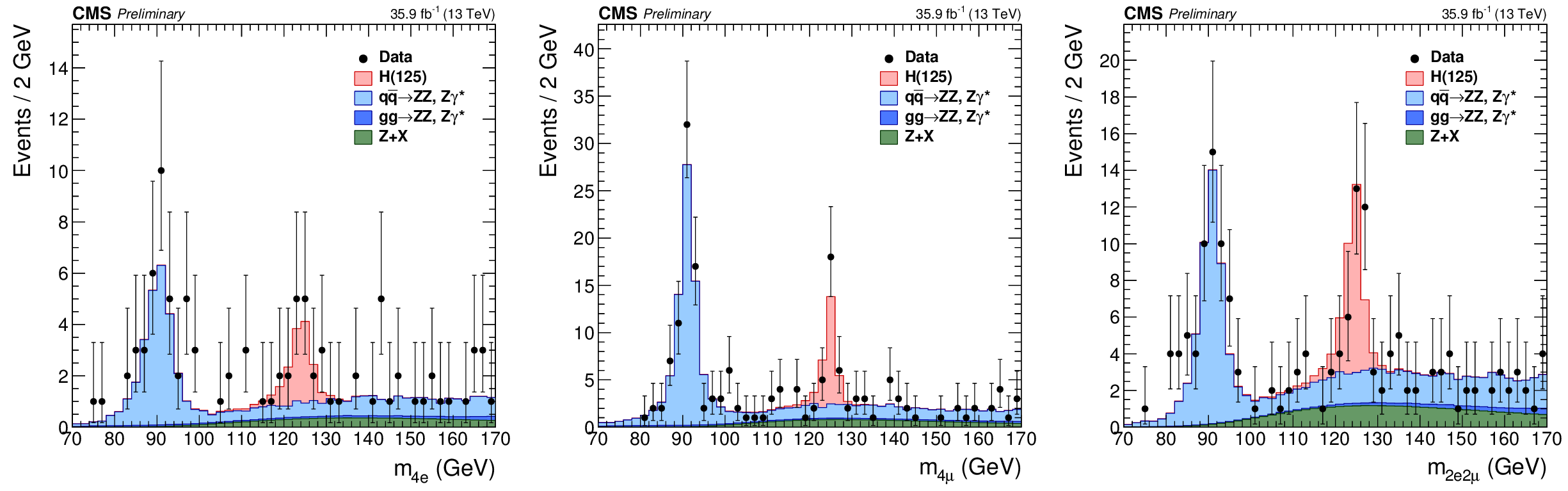
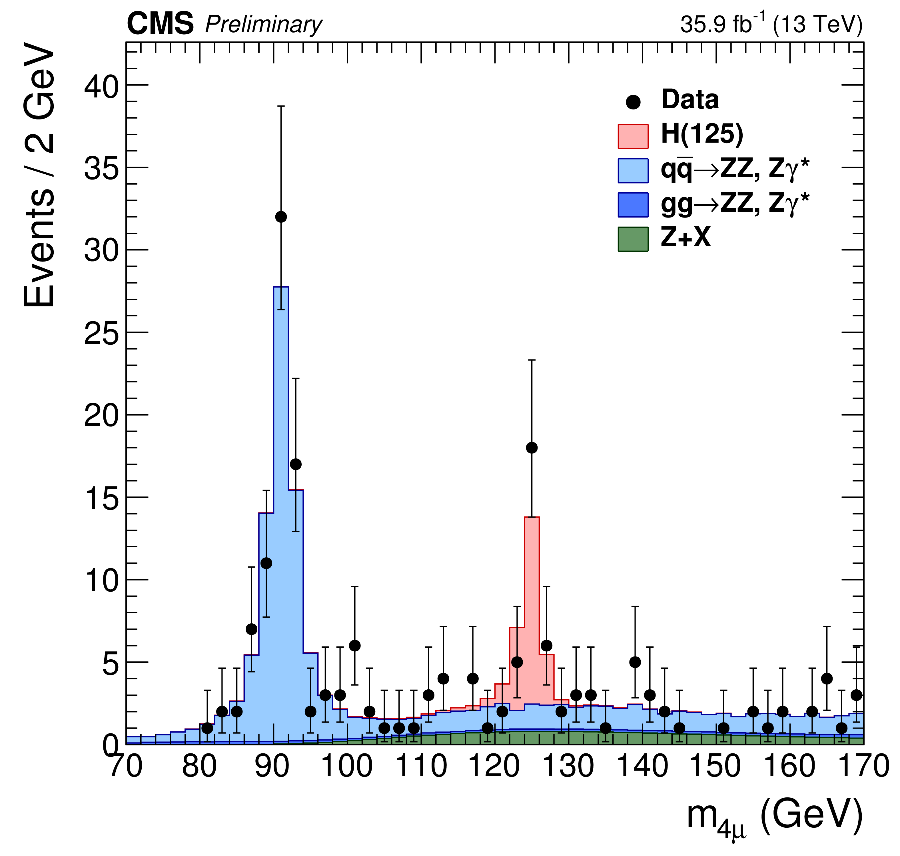
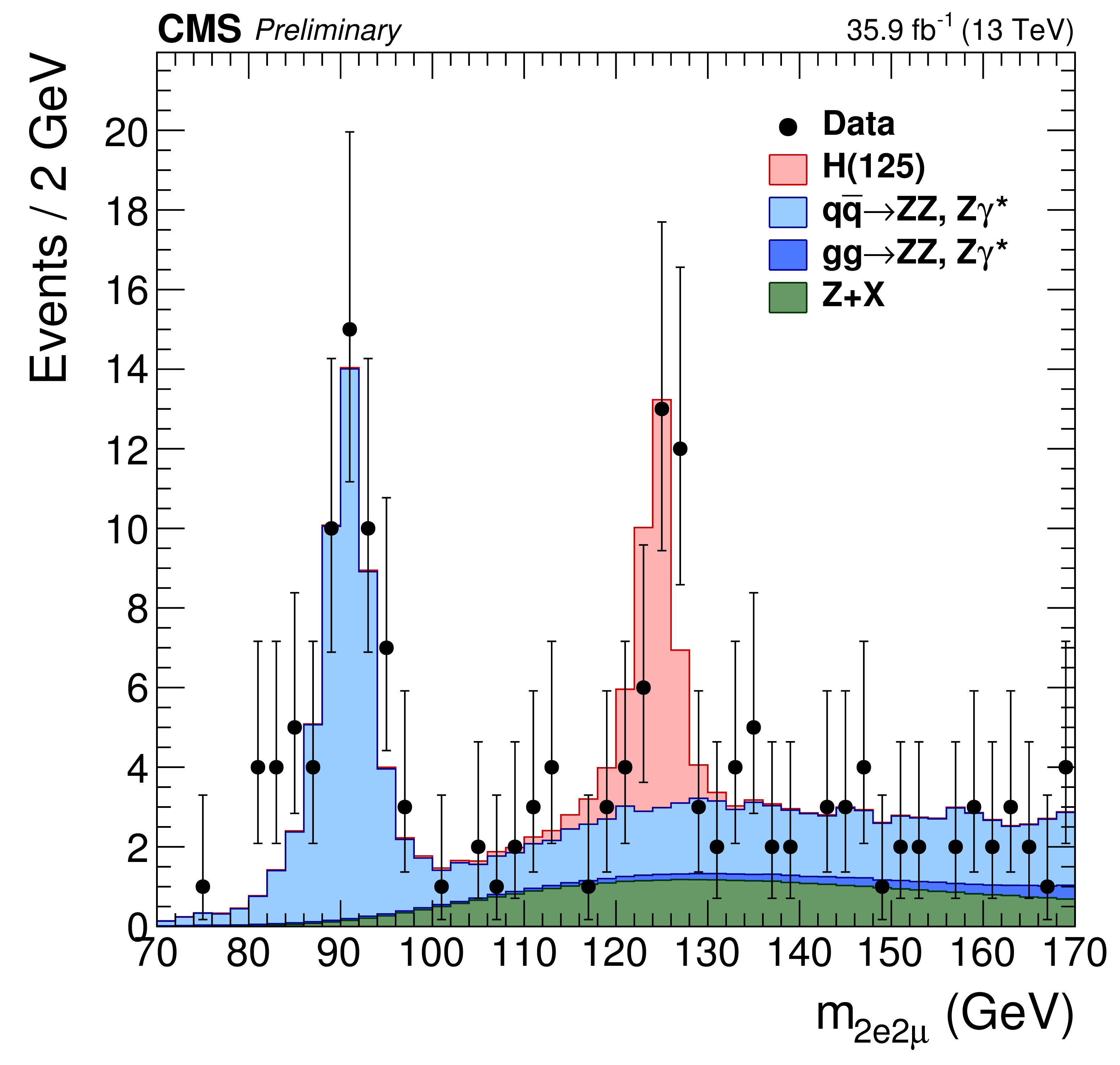
Additional Figure 1:
Distributions of $m_{4\ell }$ in the region 70 $ < m_{4\ell } < $ 170 GeV for the 4e (left), 4$\mu $ (middle) and 2e2$\mu $ (right) final states. The stacked histograms represent the expected distributions, and points represent the data. The SM Higgs boson signal with $ {m_{\mathrm{ H } }}= $ 125 GeV, denoted as H(125), and the ZZ backgrounds are normalized to the SM expectation and the Z+X background to the estimation from data. |
png pdf |
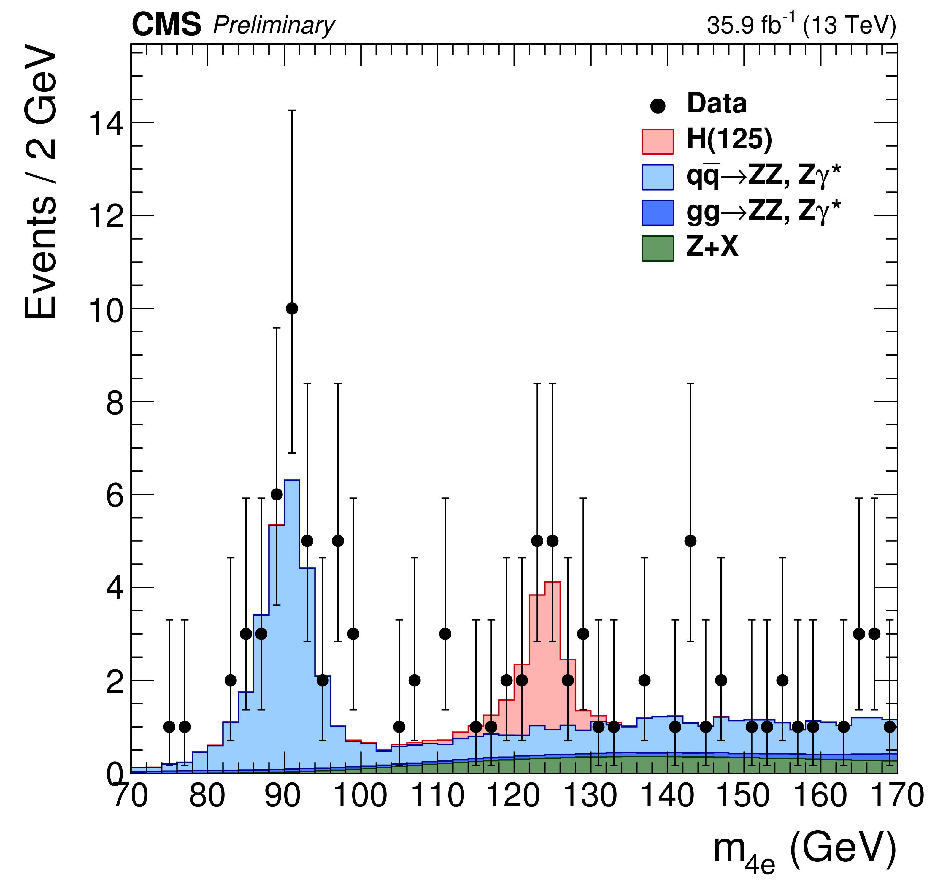
Additional Figure 1-a:
Distributions of $m_{4\ell }$ in the region 70 $ < m_{4\ell } < $ 170 GeV for the 4e final state. The stacked histograms represent the expected distributions, and points represent the data. The SM Higgs boson signal with $ {m_{\mathrm{ H } }}= $ 125 GeV, denoted as H(125), and the ZZ backgrounds are normalized to the SM expectation and the Z+X background to the estimation from data. |
png pdf |
Additional Figure 1-b:
Distributions of $m_{4\ell }$ in the region 70 $ < m_{4\ell } < $ 170 GeV for the 4$\mu $ final state. The stacked histograms represent the expected distributions, and points represent the data. The SM Higgs boson signal with $ {m_{\mathrm{ H } }}= $ 125 GeV, denoted as H(125), and the ZZ backgrounds are normalized to the SM expectation and the Z+X background to the estimation from data. |
png pdf |
Additional Figure 1-c:
Distributions of $m_{4\ell }$ in the region 70 $ < m_{4\ell } < $ 170 GeV for the 2e2$\mu $ final state. The stacked histograms represent the expected distributions, and points represent the data. The SM Higgs boson signal with $ {m_{\mathrm{ H } }}= $ 125 GeV, denoted as H(125), and the ZZ backgrounds are normalized to the SM expectation and the Z+X background to the estimation from data. |
png pdf |
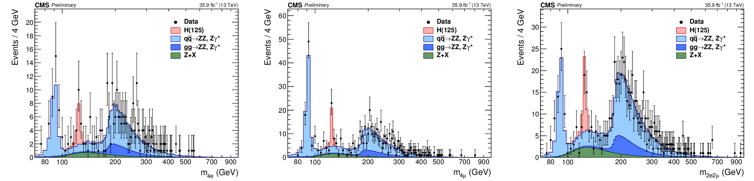
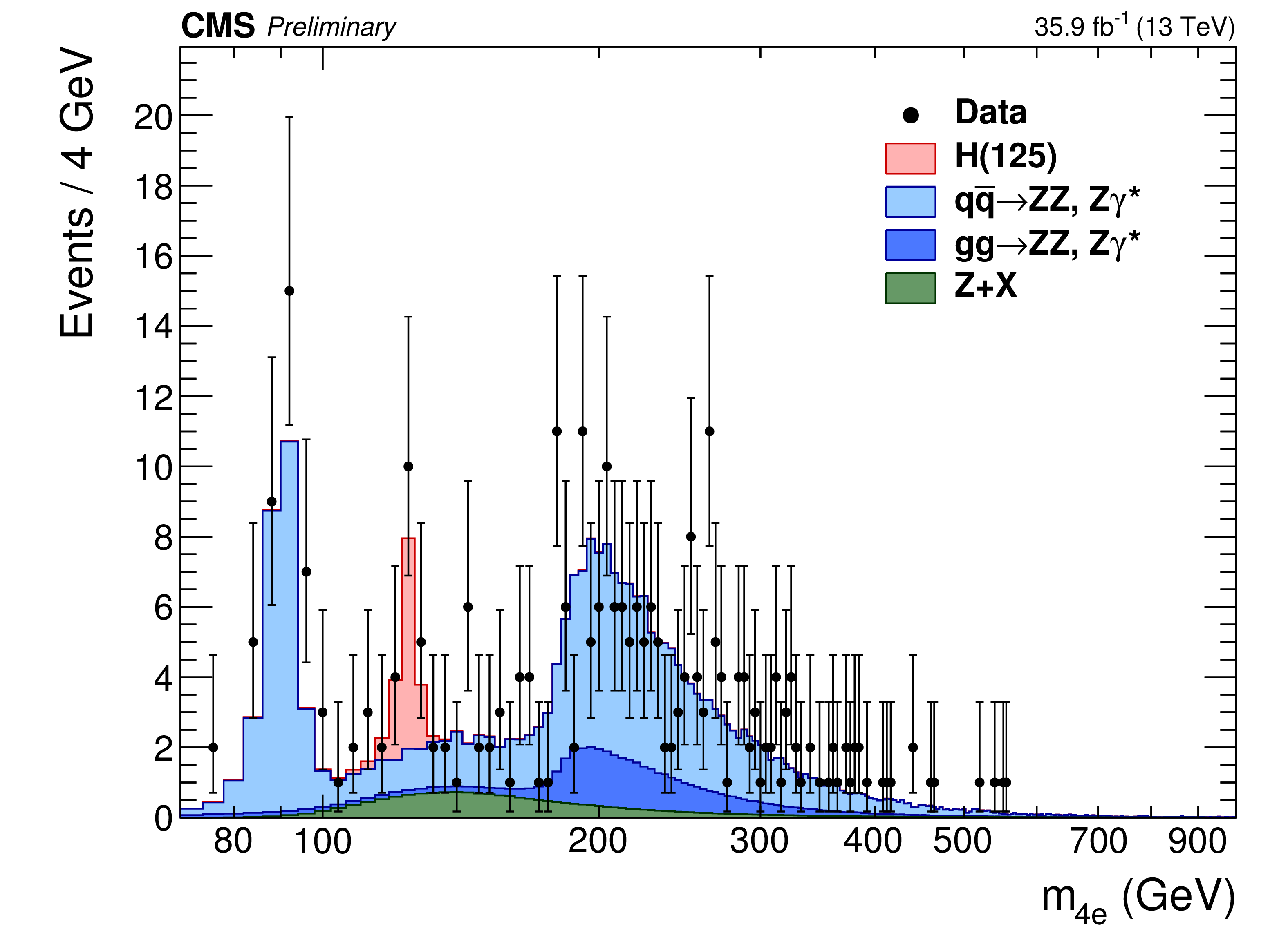
Additional Figure 2:
Distributions of $m_{4\ell }$ in the region $m_{4\ell }>$ 70 GeV for the 4e (left), 4$\mu $ (middle) and 2e2$\mu $ (right) final states. The stacked histograms represent the expected distributions, and points represent the data. The SM Higgs boson signal with $ {m_{\mathrm{ H } }}= $ 125 GeV, denoted as H(125), and the ZZ backgrounds are normalized to the SM expectation and the Z+X background to the estimation from data. |
png pdf |
Additional Figure 2-a:
Distributions of $m_{4\ell }$ in the region $m_{4\ell }>$ 70 GeV for the 4e final states. The stacked histograms represent the expected distributions, and points represent the data. The SM Higgs boson signal with $ {m_{\mathrm{ H } }}= $ 125 GeV, denoted as H(125), and the ZZ backgrounds are normalized to the SM expectation and the Z+X background to the estimation from data. |
png pdf |
Additional Figure 2-b:
Distributions of $m_{4\ell }$ in the region $m_{4\ell }>$ 70 GeV for the 4$\mu $ final states. The stacked histograms represent the expected distributions, and points represent the data. The SM Higgs boson signal with $ {m_{\mathrm{ H } }}= $ 125 GeV, denoted as H(125), and the ZZ backgrounds are normalized to the SM expectation and the Z+X background to the estimation from data. |
png pdf |
Additional Figure 2-c:
Distributions of $m_{4\ell }$ in the region $m_{4\ell }>$ 70 GeV for the 2e2$\mu $ final states. The stacked histograms represent the expected distributions, and points represent the data. The SM Higgs boson signal with $ {m_{\mathrm{ H } }}= $ 125 GeV, denoted as H(125), and the ZZ backgrounds are normalized to the SM expectation and the Z+X background to the estimation from data. |
png pdf |
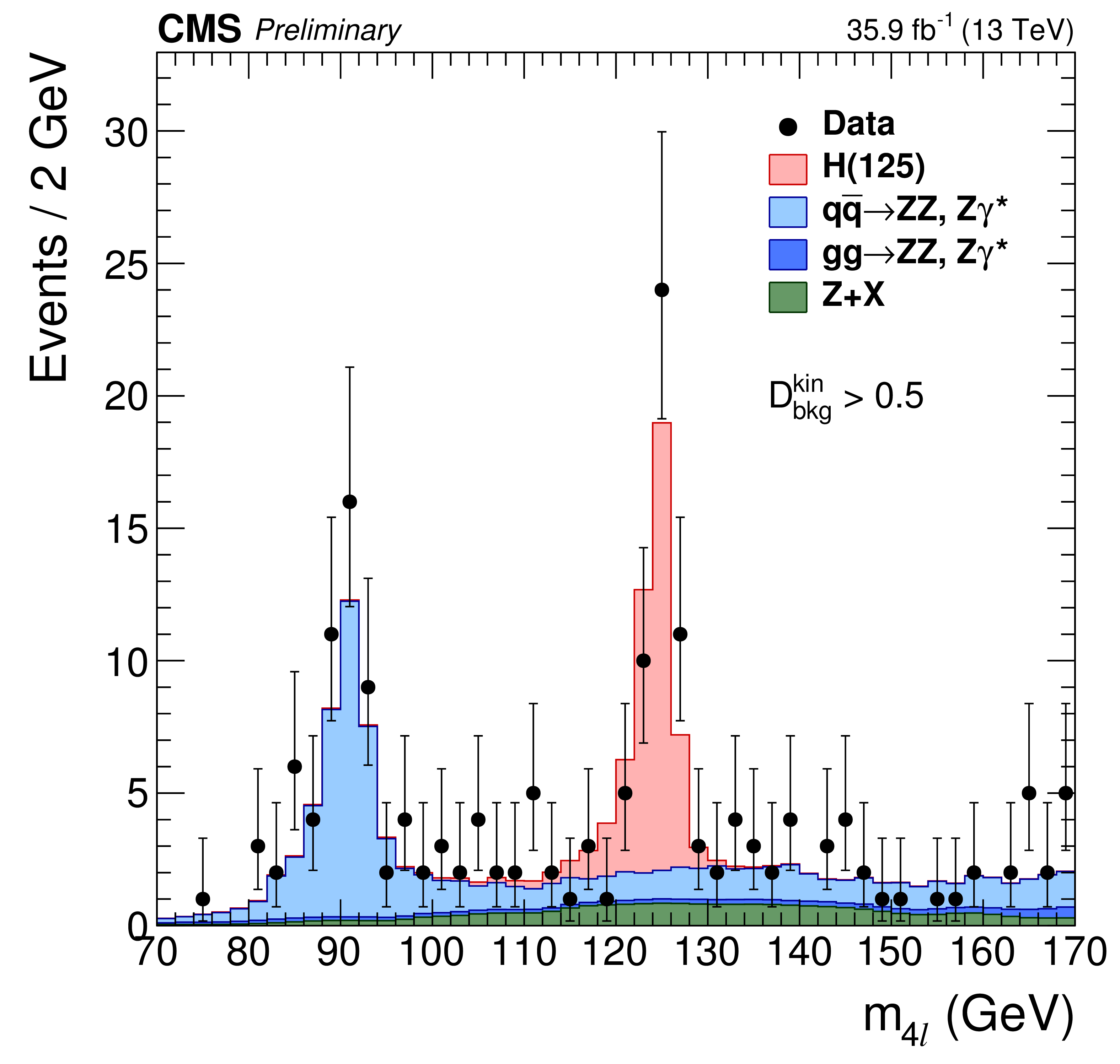
Additional Figure 3:
Distribution of $m_{4\ell }$ in the region 70 $ < m_{4\ell } < $ 170 GeV after requiring ${\cal D}^{\rm kin}_{\rm bkg}> $ 0.5. The stacked histograms represent the expected distributions, and points represent the data. The SM Higgs boson signal with $ {m_{\mathrm{ H } }}= $ 125 GeV, denoted as H(125), and the ZZ backgrounds are normalized to the SM expectation and the Z+X background to the estimation from data. |
png pdf |
Additional Figure 4:
Distribution of the $\mathrm{ Z } _1$ (a) and $\mathrm{ Z } _2$ (b) reconstructed invariant masses in the region $m_{4\ell }>$ 70 GeV. The stacked histograms represent expected distributions, and points represent the data. The SM Higgs boson signal with $ {m_{\mathrm{ H } }}= $ 125 GeV, denoted as H(125), and the ZZ backgrounds are normalized to the SM expectation and the Z+X background to the estimation from data. (c) Correlation between the reconstructed invariant masses $\mathrm{ Z } _1$ and $\mathrm{ Z } _2$ in the region $m_{4\ell }>$ 70 GeV. The gray scale represents the expected total number of ZZ background and Higgs boson signal events for $m_{\rm H}= $ 125 GeV. |
png pdf |
Additional Figure 4-a:
Distribution of the $\mathrm{ Z } _1$ reconstructed invariant masses in the region $m_{4\ell }>$ 70 GeV. The stacked histograms represent expected distributions, and points represent the data. The SM Higgs boson signal with $ {m_{\mathrm{ H } }}= $ 125 GeV, denoted as H(125), and the ZZ backgrounds are normalized to the SM expectation and the Z+X background to the estimation from data. |
png pdf |
Additional Figure 4-b:
Distribution of the $\mathrm{ Z } _2$ reconstructed invariant masses in the region $m_{4\ell }>$ 70 GeV. The stacked histograms represent expected distributions, and points represent the data. The SM Higgs boson signal with $ {m_{\mathrm{ H } }}= $ 125 GeV, denoted as H(125), and the ZZ backgrounds are normalized to the SM expectation and the Z+X background to the estimation from data. |
png pdf |
Additional Figure 4-c:
Correlation between the reconstructed invariant masses $\mathrm{ Z } _1$ and $\mathrm{ Z } _2$ in the region $m_{4\ell }>$ 70 GeV. The gray scale represents the expected total number of ZZ background and Higgs boson signal events for $m_{\rm H}= $ 125 GeV. |
png pdf |
Additional Figure 5:
(a) Distribution of ${\cal D}^{\rm kin}_{\rm bkg}$ in the region $m_{4\ell }>$ 70 GeV. The stacked histograms represent the expected distributions, and points represent the data. The SM Higgs boson signal with $ {m_{\mathrm{ H } }}= $ 125 GeV, denoted as H(125), and the ZZ backgrounds are normalized to the SM expectation and the Z+X background to the estimation from data. (b) 2D distribution of ${\cal D}^{\rm kin}_{\rm bkg}$ vs $m_{4\ell }$ in the region 170 $ < m_{4\ell } < $ 1000 GeV. The gray scale represents the expected total number of ZZ background and Higgs boson signal events for $m_{\rm H}= $ 125 GeV. The points show the data and the horizontal bars represent the measured event-by-event mass uncertainties. |
png pdf |
Additional Figure 5-a:
Distribution of ${\cal D}^{\rm kin}_{\rm bkg}$ in the region $m_{4\ell }>$ 70 GeV. The stacked histograms represent the expected distributions, and points represent the data. The SM Higgs boson signal with $ {m_{\mathrm{ H } }}= $ 125 GeV, denoted as H(125), and the ZZ backgrounds are normalized to the SM expectation and the Z+X background to the estimation from data. |
png pdf |
Additional Figure 5-b:
2D distribution of ${\cal D}^{\rm kin}_{\rm bkg}$ vs $m_{4\ell }$ in the region 170 $ < m_{4\ell } < $ 1000 GeV. The gray scale represents the expected total number of ZZ background and Higgs boson signal events for $m_{\rm H}= $ 125 GeV. The points show the data and the horizontal bars represent the measured event-by-event mass uncertainties. |
png pdf |
Additional Figure 6:
2D distributions of ${\mathcal D}_{\rm 1jet}$ (a), ${\mathcal D}_{\rm 2jet}$ (b), ${\mathcal D}_{\rm VH}$ (c) vs $m_{4\ell }$ in the region 100$ < m_{4\ell } < $ 170 GeV. The gray scale represents the expected relative density of ZZ background plus Higgs boson signal for$m_{\rm H}= $ 125 GeV. The points show the data and the horizontal bars represent the measured event-by-event mass uncertainties. The gray dashed lines denote the working points used in the event categorization and different marker styles are used to denote the final categorization of the events. |
png pdf |
Additional Figure 6-a:
2D distribution of ${\mathcal D}_{\rm 1jet}$ vs $m_{4\ell }$ in the region 100 $ < m_{4\ell } < $ 170 GeV. The gray scale represents the expected relative density of ZZ background plus Higgs boson signal for$m_{\rm H}= $ 125 GeV. The points show the data and the horizontal bars represent the measured event-by-event mass uncertainties. The gray dashed lines denote the working points used in the event categorization and different marker styles are used to denote the final categorization of the events. |
png pdf |
Additional Figure 6-b:
2D distribution of ${\mathcal D}_{\rm 2jet}$ s $m_{4\ell }$ in the region 100 $ < m_{4\ell } < $ 170 GeV. The gray scale represents the expected relative density of ZZ background plus Higgs boson signal for$m_{\rm H}= $ 125 GeV. The points show the data and the horizontal bars represent the measured event-by-event mass uncertainties. The gray dashed lines denote the working points used in the event categorization and different marker styles are used to denote the final categorization of the events. |
png pdf |
Additional Figure 6-c:
2D distribution of ${\mathcal D}_{\rm VH}$ vs $m_{4\ell }$ in the region 100 $ < m_{4\ell } < $ 170 GeV. The gray scale represents the expected relative density of ZZ background plus Higgs boson signal for$m_{\rm H}= $ 125 GeV. The points show the data and the horizontal bars represent the measured event-by-event mass uncertainties. The gray dashed lines denote the working points used in the event categorization and different marker styles are used to denote the final categorization of the events. |
png pdf |
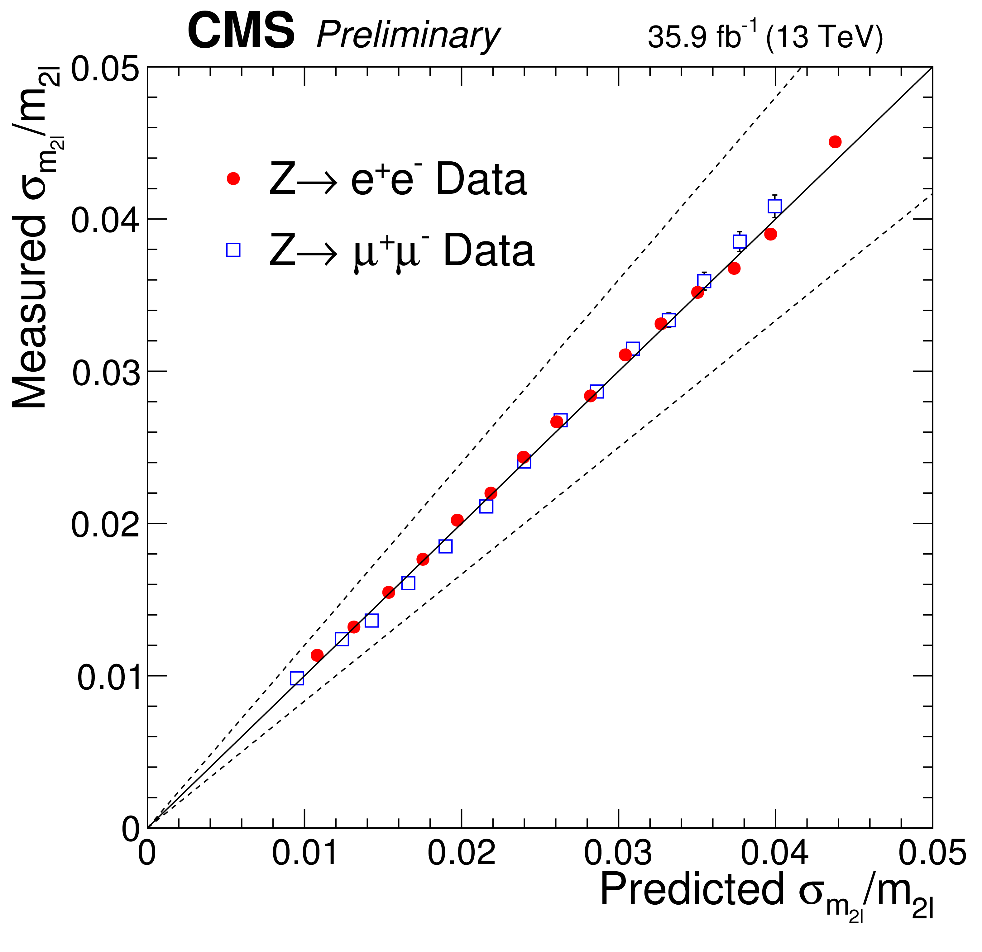
Additional Figure 7:
Comparison of measured mass resolution with the predicted dilepton mass resolution using the event-by-event mass uncertainty for $\mathrm{ Z } \to \ell \ell $ events in data. The dashed lines denote a $\pm$20% region, used as the systematic uncertainty on the resolution. |
png pdf |
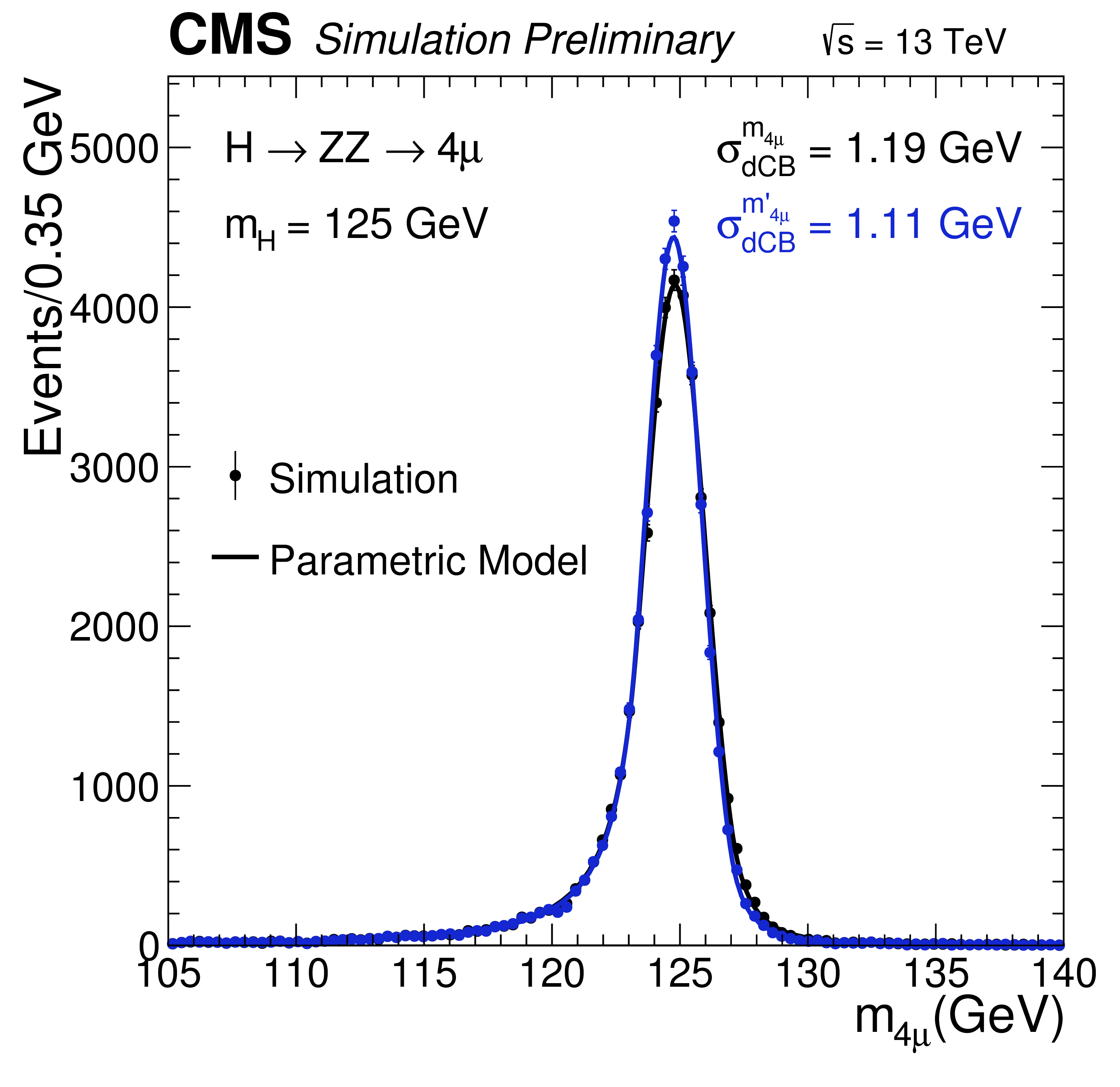
Additional Figure 8:
Comparison of the four-lepton mass for simulated Higgs boson events with $m_{\rm H}= $ 125 GeV in the 4$\mu $ final state with and without the kinematic refit using $m({\rm Z}_1)$ constraint. |
png pdf |
Additional Figure 9:
Comparison of the four-lepton mass for simulated Higgs boson events with $m_{\rm H}= $ 125 GeV in the 4e final state with and without the kinematic refit using $m({\rm Z}_1)$ constraint. |
png pdf |
Additional Figure 10:
Comparison of the four-lepton mass for simulated Higgs boson events with $m_{\rm H}= $ 125 GeV in the 2e2$\mu $ final state with and without the kinematic refit using $m({\rm Z}_1)$ constraint. |
png pdf |
Additional Figure 11:
Four lepton mass distribution using the full CMS datasets from $\sqrt {s}= $ 7, 8 and 13 TeV . The stacked histograms represent the expected distributions, and points represent the data. The SM Higgs boson signal with $ {m_{\mathrm{ H } }}= $ 125 GeV, denoted as H(125), and the ZZ backgrounds are normalized to the SM expectation and the Z+X background to the estimation from data. |
| References | ||||
| 1 | CMS Collaboration | Observation of a new boson at a mass of 125 GeV with the CMS experiment at the LHC | PLB 716 (2012) 30 | CMS-HIG-12-028 1207.7235 |
| 2 | ATLAS Collaboration | Observation of a new particle in the search for the Standard Model Higgs boson with the ATLAS detector at the LHC | PLB 716 (2012) 1 | 1207.7214 |
| 3 | F. Englert and R. Brout | Broken Symmetry and the Mass of Gauge Vector Mesons | PRL 13 (1964) 321 | |
| 4 | P. W. Higgs | Broken symmetries, massless particles and gauge fields | PL12 (1964) 132 | |
| 5 | P. W. Higgs | Broken Symmetries and the Masses of Gauge Bosons | PRL 13 (1964) 508 | |
| 6 | G. Guralnik, C. Hagen, and T. Kibble | Global Conservation Laws and Massless Particles | PRL 13 (1964) 585 | |
| 7 | P. W. Higgs | Spontaneous Symmetry Breakdown without Massless Bosons | PR145 (1966) 1156 | |
| 8 | T. Kibble | Symmetry breaking in nonAbelian gauge theories | PR155 (1967) 1554 | |
| 9 | CMS Collaboration | Precise determination of the mass of the Higgs boson and tests of compatibility of its couplings with the standard model predictions using proton collisions at 7 and 8 TeV | EPJC 75 (2015) 212 | CMS-HIG-14-009 1412.8662 |
| 10 | ATLAS Collaboration | Measurements of the Higgs boson production and decay rates and coupling strengths using $ pp $ collision data at $ \sqrt{s}= $ 7 and 8 TeV in the ATLAS experiment | EPJC 76 (2016) | 1507.04548 |
| 11 | ATLAS and CMS Collaborations | Combined Measurement of the Higgs Boson Mass in $ pp $ Collisions at $ \sqrt{s}= $ 7 and 8 TeV with the ATLAS and CMS Experiments | PRL 114 (2015) 191803 | 1503.07589 |
| 12 | ATLAS and CMS Collaborations | Measurements of the Higgs boson production and decay rates and constraints on its couplings from a combined ATLAS and CMS analysis of the LHC pp collision data at $ \sqrt{s}= $ 7 and 8 TeV | JHEP 08 (2016) 45 | 1606.02266 |
| 13 | CMS Collaboration | Measurement of the properties of a Higgs boson in the four-lepton final state | PRD 89 (2014) 092007 | CMS-HIG-13-002 1312.5353 |
| 14 | CMS Collaboration | Study of the Mass and Spin-Parity of the Higgs Boson Candidate via Its Decays to $ Z $ Boson Pairs | PRL 110 (2013) 081803 | CMS-HIG-12-041 1212.6639 |
| 15 | CMS Collaboration | Constraints on the spin-parity and anomalous HVV couplings of the Higgs boson in proton collisions at 7 and 8 TeV | PRD 92 (2015) 012004 | CMS-HIG-14-018 1411.3441 |
| 16 | CMS Collaboration | Constraints on the Higgs boson width from off-shell production and decay to $ \mathrm{ Z } $-boson pairs | PLB 736 (2014) 64 | CMS-HIG-14-002 1405.3455 |
| 17 | CMS Collaboration | Limits on the Higgs boson lifetime and width from its decay to four charged leptons | PRD 92 (2015) 072010 | CMS-HIG-14-036 1507.06656 |
| 18 | CMS Collaboration | Measurement of differential and integrated fiducial cross sections for Higgs boson production in the four-lepton decay channel in pp collisions at $ \sqrt{s}= $ 7 and 8 TeV | JHEP 04 (2016) 005 | CMS-HIG-14-028 1512.08377 |
| 19 | CMS Collaboration | The CMS experiment at the CERN LHC | JINST 3 (2008) S08004 | CMS-00-001 |
| 20 | S. Alioli, P. Nason, C. Oleari, and E. Re | NLO vector-boson production matched with shower in POWHEG | JHEP 07 (2008) 060 | 0805.4802 |
| 21 | P. Nason | A new method for combining NLO QCD with shower Monte Carlo algorithms | JHEP 11 (2004) 040 | hep-ph/0409146 |
| 22 | S. Frixione, P. Nason, and C. Oleari | Matching NLO QCD computations with parton shower simulations: the POWHEG method | JHEP 11 (2007) 070 | 0709.2092 |
| 23 | G. Luisoni, P. Nason, C. Oleari, and F. Tramontano | HW$ ^{\pm} $/HZ + 0 and 1 jet at NLO with the POWHEG BOX interfaced to GoSam and their merging within MiNLO | JHEP 10 (2013) 1 | 1306.2542 |
| 24 | C. Anastasiou et al. | High precision determination of the gluon fusion Higgs boson cross-section at the LHC | JHEP 2016 (2016), no. 5, 1 | 1602.00695 |
| 25 | R. Ball et al. | Unbiased global determination of parton distributions and their uncertainties at NNLO and at LO | Nucl. Phys. B 855 (2012), no. 2, 153 | 1107.2652 |
| 26 | Y. Gao et al. | Spin determination of single-produced resonances at hadron colliders | PRD 81 (2010) 075022 | 1001.3396 |
| 27 | S. Bolognesi et al. | On the spin and parity of a single-produced resonance at the LHC | PRD 86 (2012) 095031 | 1208.4018 |
| 28 | J. M. Campbell and R. K. Ellis | MCFM for the Tevatron and the LHC | NPPS 205 (2010) 10 | 1007.3492 |
| 29 | T. Sjostrand et al. | An introduction to PYTHIA 8.2 | Computer Physics Communications 191 (2015) 159 | |
| 30 | GEANT4 Collaboration | GEANT4: a simulation toolkit | NIMA 506 (2003) 250 | |
| 31 | J. Allison et al. | Geant4 developments and applications | IEEE Trans. Nucl. Sci. 53 (2006) 270 | |
| 32 | CMS Collaboration | Particle-flow event reconstruction in CMS and performance for jets, taus, and $ E_{\mathrm{T}}^{\text{miss}} $ | CDS | |
| 33 | CMS Collaboration | Commissioning of the particle-flow event with the first LHC collisions recorded in the CMS detector | CDS | |
| 34 | CMS Collaboration | Performance of electron reconstruction and selection with the CMS detector in proton-proton collisions at $ \sqrt{s} = $ 8 TeV | JINST 10 (2015) P06005 | CMS-EGM-13-001 1502.02701 |
| 35 | CMS Collaboration | Performance of CMS muon reconstruction in $ pp $ collision events at $ \sqrt{s} = $ 7 TeV | JINST 7 (2012) P10002 | CMS-MUO-10-004 1206.4071 |
| 36 | CMS Collaboration | W-like measurement of the Z boson mass using dimuon events collected in pp collisions at $ \sqrt{s}= $ 7 TeV | ||
| 37 | M. Cacciari, G. P. Salam, and G. Soyez | The anti-$ k_t $ jet clustering algorithm | JHEP 04 (2008) 063 | 0802.1189 |
| 38 | M. Cacciari, G. P. Salam, and G. Soyez | FastJet user manual | EPJC 72 (2012) 1896 | 1111.6097 |
| 39 | CMS Collaboration | Determination of jet energy calibration and transverse momentum resolution in CMS | JINST 6 (2011) P11002 | CMS-JME-10-011 1107.4277 |
| 40 | Particle Data Group Collaboration | Review of Particle Physics | CPC40 (2016), no. 10, 100001 | |
| 41 | I. Anderson et al. | Constraining anomalous $ HVV $ interactions at proton and lepton colliders | PRD 89 (2014) 035007 | 1309.4819 |
| 42 | CMS Collaboration | Search for a Higgs Boson in the Mass Range from 145 to 1000 GeV Decaying to a Pair of W or Z Bosons | JHEP 10 (2015) 144 | CMS-HIG-13-031 1504.00936 |
| 43 | M. Grazzini, S. Kallweit, and D. Rathlev | ZZ production at the LHC: Fiducial cross sections and distributions in NNLO QCD | PLB 750 (2015) 407 -- 410 | 1507.06257 |
| 44 | M. Bonvini et al. | Signal-background interference effects in $ gg \to H \to WW $ beyond leading order | PRD 88 (2013) 034032 | 1304.3053 |
| 45 | K. Melnikov and M. Dowling | Production of two Z-bosons in gluon fusion in the heavy top quark approximation | PLB 744 (2015) 43 | 1503.01274 |
| 46 | C. S. Li, H. T. Li, D. Y. Shao, and J. Wang | Soft gluon resummation in the signal-background interference process of $ gg(\to h^*) \to ZZ $~ | 1504.02388 | |
| 47 | G. Passarino | Higgs CAT | EPJC 74 (2014) 2866 | 1312.2397 |
| 48 | S. Catani and M. Grazzini | An NNLO subtraction formalism in hadron collisions and its application to Higgs boson production at the LHC | PRL 98 (2007) 222002 | hep-ph/0703012 |
| 49 | M. Grazzini | NNLO predictions for the Higgs boson signal in the H $ \to $ WW $ \to\ell\nu\ell\nu $ and H$ \to $ ZZ $ \to4\ell $ decay channels | JHEP 02 (2008) 043 | 0801.3232 |
| 50 | M. Grazzini and H. Sargsyan | Heavy-quark mass effects in Higgs boson production at the LHC | JHEP 09 (2013) 129 | 1306.4581 |
| 51 | L. Landau | On the energy loss of fast particles by ionization | J. Phys. (USSR) 8 (1944)201 | |
| 52 | D. de Florian, G. Ferrera, M. Grazzini, and D. Tommasini | Higgs boson production at the LHC: transverse momentum resummation effects in the $ H \to \gamma \gamma $, $ H \to WW \to \ell\nu\ell\nu $ and $ H \to ZZ \to 4\ell $ decay modes | JHEP 06 (2012) 132 | 1203.6321 |
| 53 | LHC Higgs Cross Section Working Group | Handbook of LHC Higgs Cross Sections: 4. Deciphering the Nature of the Higgs Sector | CERN-2016-XXX (CERN, Geneva, 2016) | 1610.07922 |
| 54 | R. D. Cousins | Why isn't every physicist a Bayesian? | Am. J. Phys. 63 (1995) 398 | |
| 55 | ATLAS and CMS Collaborations, LHC Higgs Combination Group | Procedure for the LHC Higgs boson search combination in Summer 2011 | ATL-PHYS-PUB/CMS NOTE 2011-11, 2011/005, CERN | |
| 56 | G. Cowan, K. Cranmer, E. Gross, and O. Vitells | Asymptotic formulae for likelihood-based tests of new physics | EPJC 71 (2011) 1554 | 1007.1727 |
| 57 | CMS Collaboration | Measurement of differential cross sections for Higgs boson production in the diphoton decay channel in pp collisions at $ \sqrt{s} = $ 8 TeV | EPJC 76 (2015) 13 | CMS-HIG-14-016 1508.07819 |
|
|
Compact Muon Solenoid LHC, CERN |
|

|

|

|

|

|