

Compact Muon Solenoid
LHC, CERN
| CMS-PAS-TOP-17-004 | ||
| Constraining the top quark Yukawa coupling from $\text{t}\bar{\text{t}}$ differential cross sections in the lepton+jets final state in proton-proton collisions at $\sqrt{s}= $ 13 TeV | ||
| CMS Collaboration | ||
| March 2019 | ||
| Abstract: A measurement of the top quark Yukawa coupling from the top quark-antiquark ($\text{t}\bar{\text{t}}$) differential production cross sections in proton-proton collisions with the lepton+jets channel is presented. Corrections due to electroweak bosons exchange, including the Higgs boson, between the final state top quarks can produce large distortions of differential distributions near the energy threshold of top quark pair production. Therefore precise measurements of these distributions are sensitive to the Yukawa coupling. This analysis is based on data collected by the CMS experiment at the LHC at $\sqrt{s}= $ 13 TeV corresponding to an integrated luminosity of 35.8 fb$^{-1}$. Top quark events are reconstructed with at least three jets in the final state. A novel technique is introduced to reconstruct the $\text{t}\bar{\text{t}}$ system for events with one missing jet. This technique enhances the experimental sensitivity in the low invariant mass region, $M_{\text{t}\bar{\text{t}}}$. The data yields in $M_{\text{t}\bar{\text{t}}}$, the rapidity difference $|y_\text{t}-y_{\bar{\text{t}}}|$, and the number of reconstructed jets are compared with distributions representing different Yukawa couplings. These comparisons are used to extract an upper limit on the top quark Yukawa coupling of 1.67 (1.62 expected) at 95% confidence level. | ||
|
Links:
CDS record (PDF) ;
CADI line (restricted) ;
These preliminary results are superseded in this paper, PRD 100 (2019) 072007. The superseded preliminary plots can be found here. |
||
| Figures | |
png pdf |
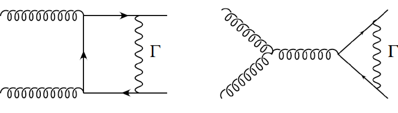
Figure 1:
Example diagrams for gluon-induced process of $ {{\mathrm {t}\overline {\mathrm {t}}}} $ production and the virtual corrections. $\Gamma $ stands for all contributions from the gauge boson, Goldstone boson and Higgs boson exchanges. |
png pdf |
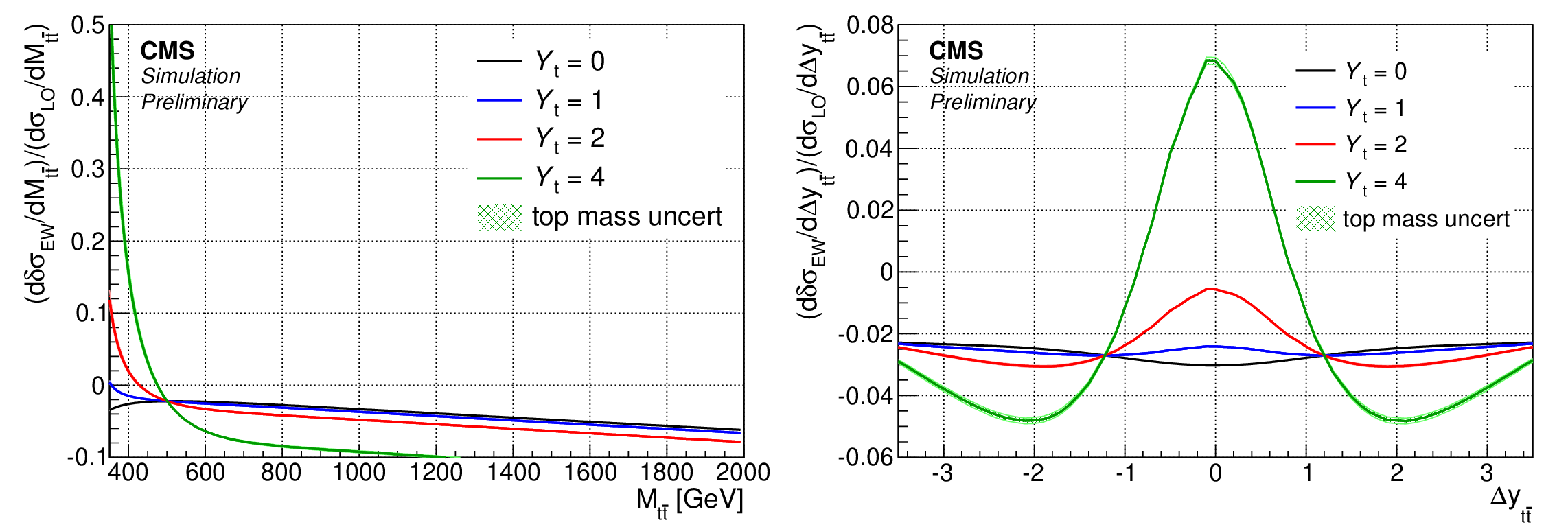
Figure 2:
The dependence of the ratio of EW correction over the leading-order production cross section on the sensitive kinematic variables ${M_{{{\mathrm {t}\overline {\mathrm {t}}}}}}$ and ${\Delta y_{{{\mathrm {t}\overline {\mathrm {t}}}}}}$ for different values of Yukawa coupling, as evaluated with HATHOR [5]. The lines contain an uncertainty band derived from the dependence of the EW correction on the top quark mass varied by $\pm $1 GeV. The effect of the top quark mass is very small at the parton level and not visible in the scale of the plot. |
png pdf |
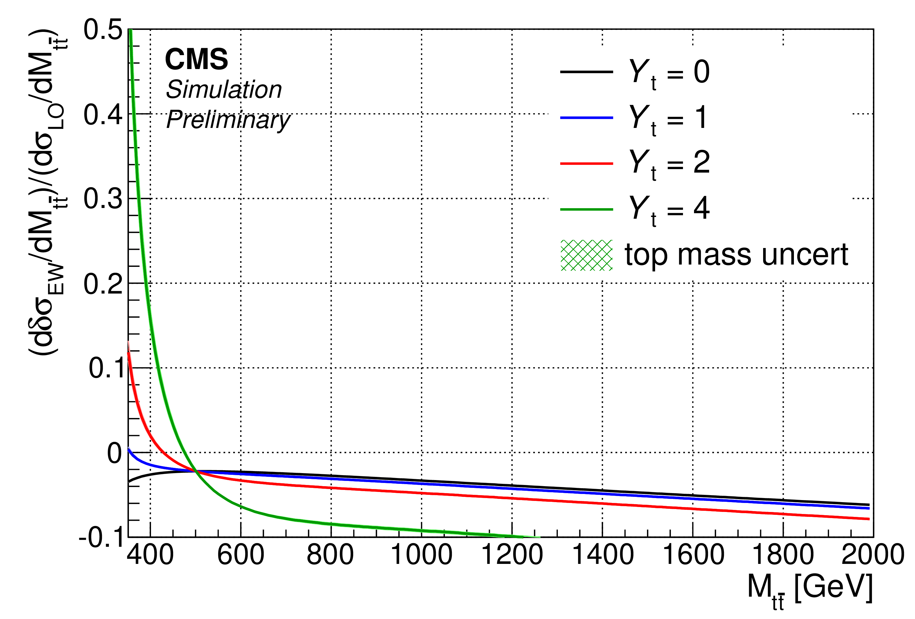
Figure 2-a:
The dependence of the ratio of EW correction over the leading-order production cross section on the kinematic variable ${M_{{{\mathrm {t}\overline {\mathrm {t}}}}}}$ for different values of Yukawa coupling, as evaluated with HATHOR [5]. The lines contain an uncertainty band derived from the dependence of the EW correction on the top quark mass varied by $\pm $1 GeV. The effect of the top quark mass is very small at the parton level and not visible in the scale of the plot. |
png pdf |
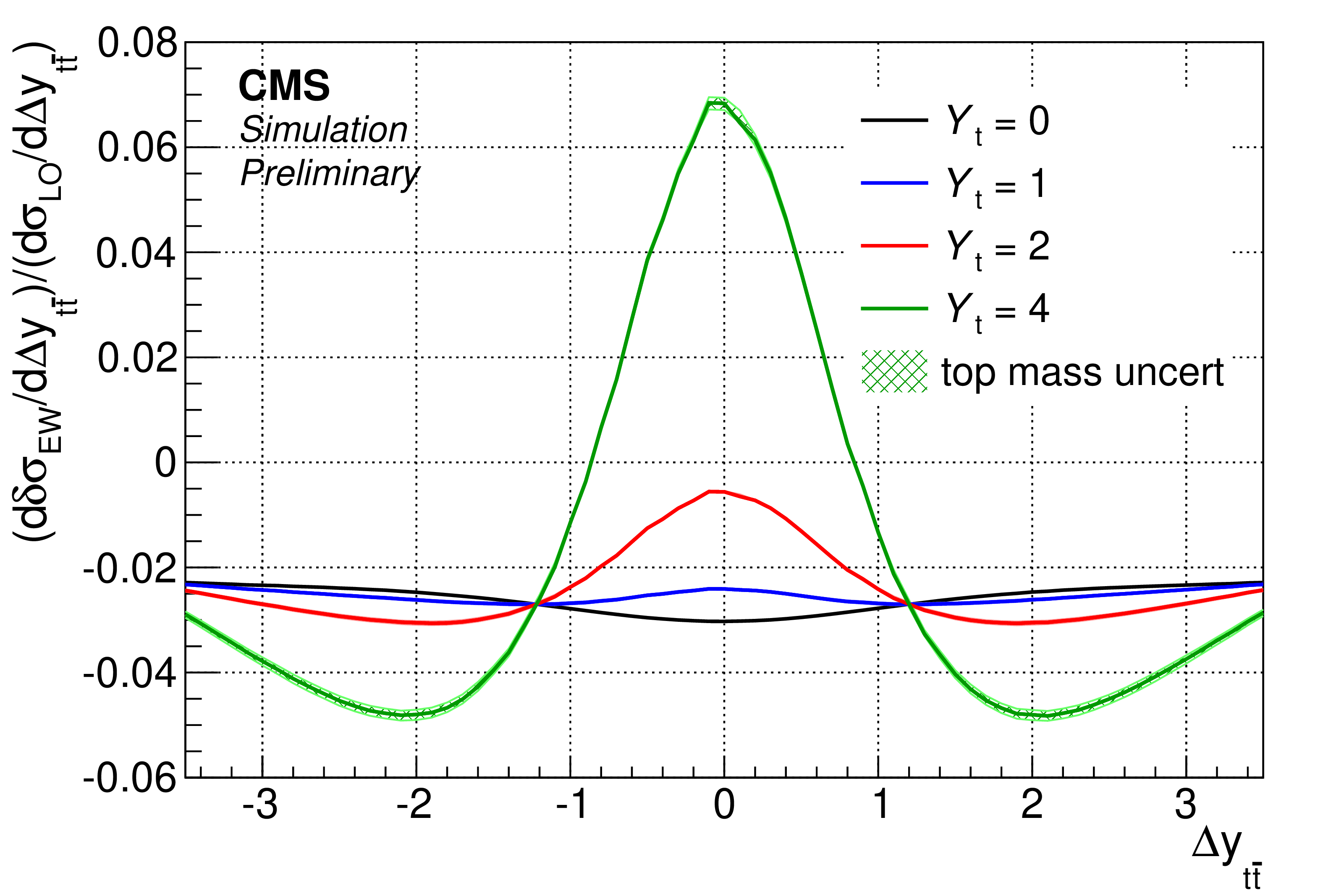
Figure 2-b:
The dependence of the ratio of EW correction over the leading-order production cross section on the kinematic variable ${\Delta y_{{{\mathrm {t}\overline {\mathrm {t}}}}}}$ for different values of Yukawa coupling, as evaluated with HATHOR [5]. The lines contain an uncertainty band derived from the dependence of the EW correction on the top quark mass varied by $\pm $1 GeV. The effect of the top quark mass is very small at the parton level and not visible in the scale of the plot. |
png pdf |
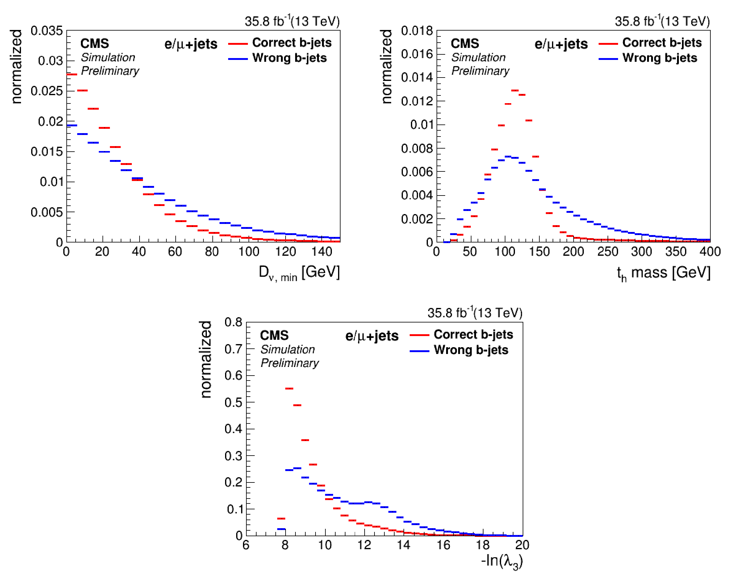
Figure 3:
Three-jet reconstruction. Upper left: normalized distributions of the distance ${D_{\nu,\mathrm {min}}}$ for correctly and wrongly selected $\mathrm {b}_{\ell}$ candidates. Upper right: normalized mass distribution of the correctly and wrongly selected $\mathrm {b}_h$ and the jet from W. Lower plot: Distribution of the negative combined log-likelihood. |
png |
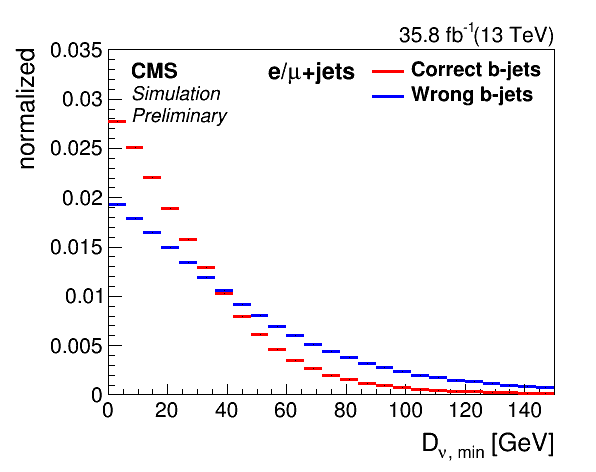
Figure 3-a:
Three-jet reconstruction. Normalized distributions of the distance ${D_{\nu,\mathrm {min}}}$ for correctly and wrongly selected $\mathrm {b}_{\ell}$ candidates. |
png |
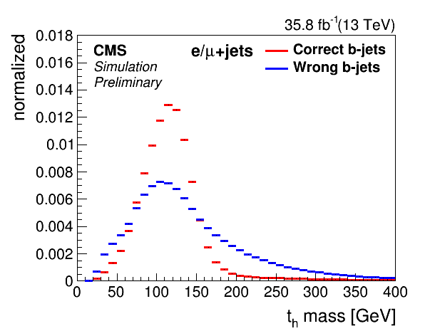
Figure 3-b:
Three-jet reconstruction. Normalized mass distribution of the correctly and wrongly selected $\mathrm {b}_h$ and the jet from W. |
png |
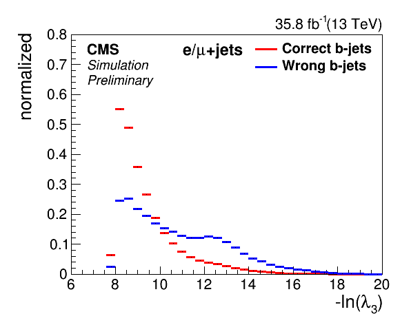
Figure 3-c:
Three-jet reconstruction. Distribution of the negative combined log-likelihood. |
png pdf |
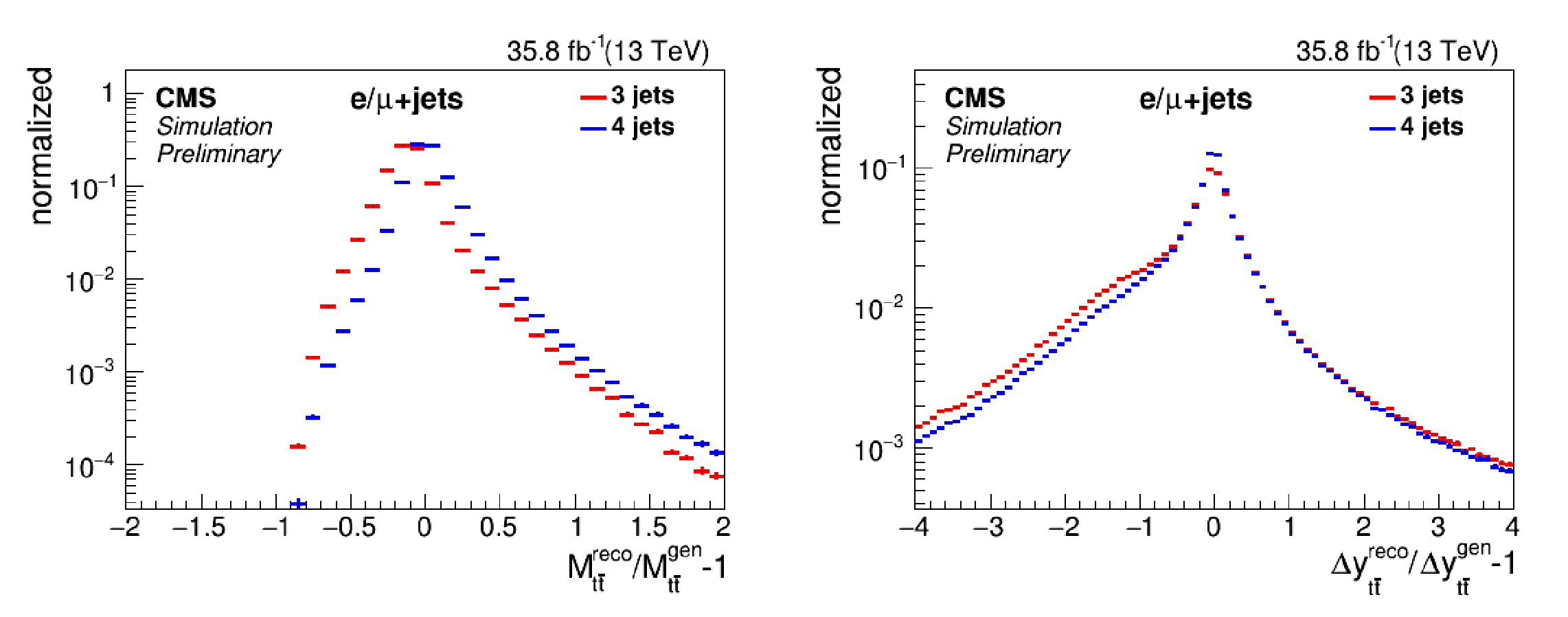
Figure 4:
Resolution of the invariant mass of the $ {{\mathrm {t}\overline {\mathrm {t}}}} $ system (left) and the difference in rapidity of top quark/antiquark (right) for three-jet and at least four-jet event categories. |
png |
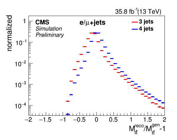
Figure 4-a:
Resolution of the invariant mass of the $ {{\mathrm {t}\overline {\mathrm {t}}}} $ system for three-jet and at least four-jet event categories. |
png |
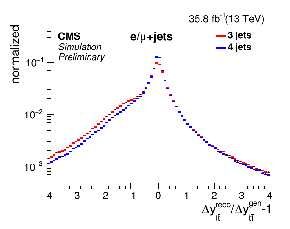
Figure 4-b:
Resolution of the difference in rapidity of top quark/antiquark for three-jet and at least four-jet event categories. |

png pdf |
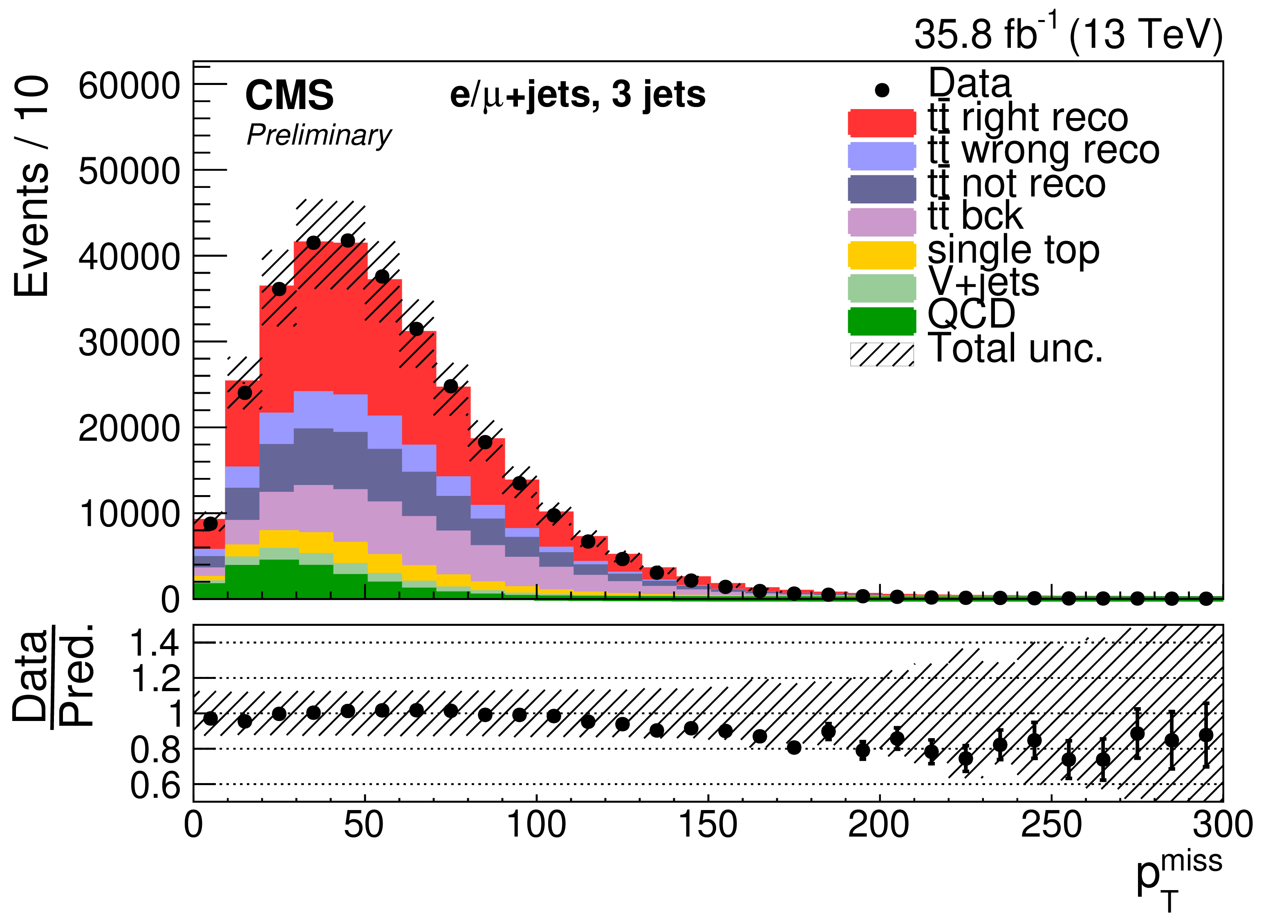
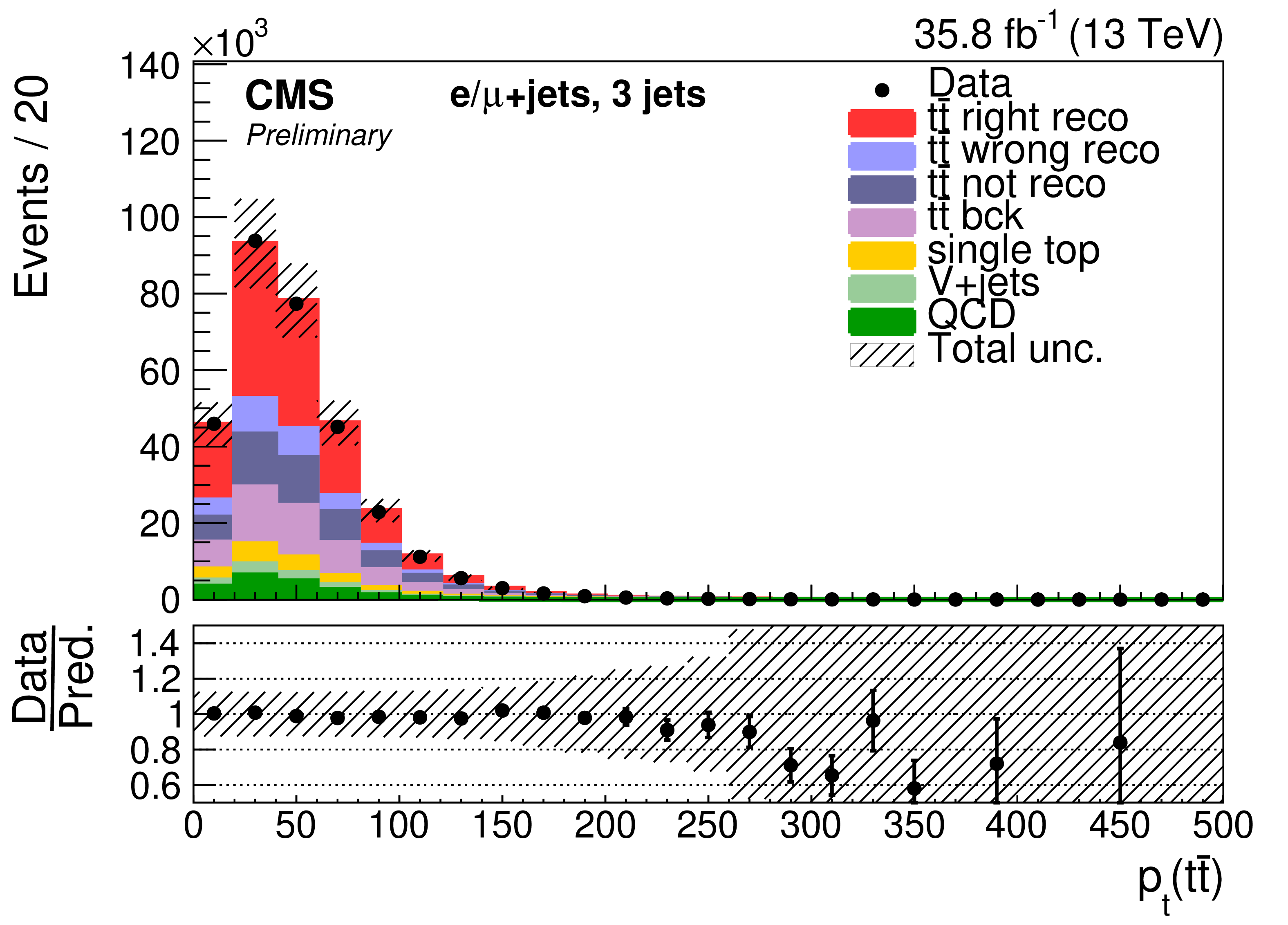
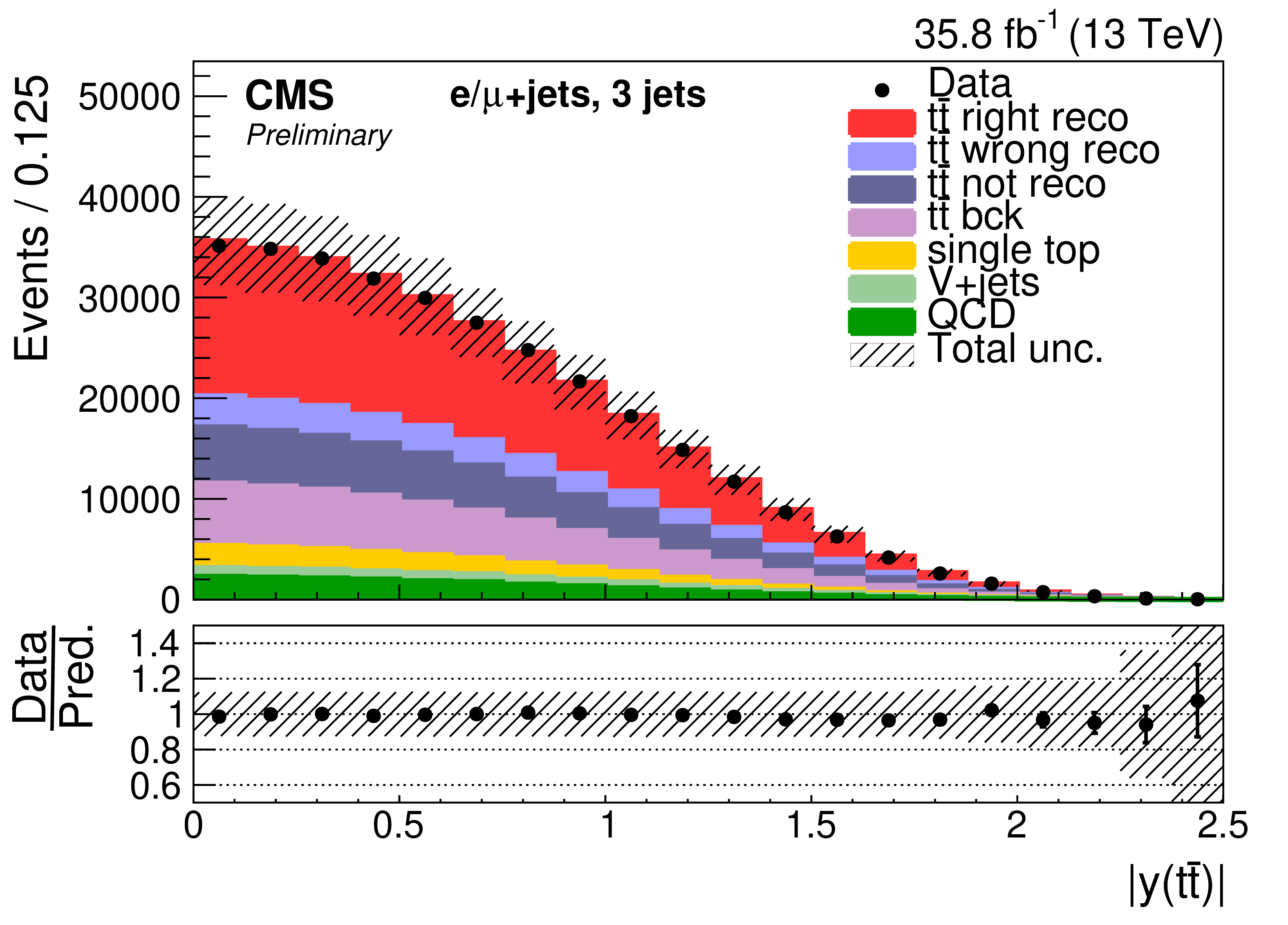
Figure 5:
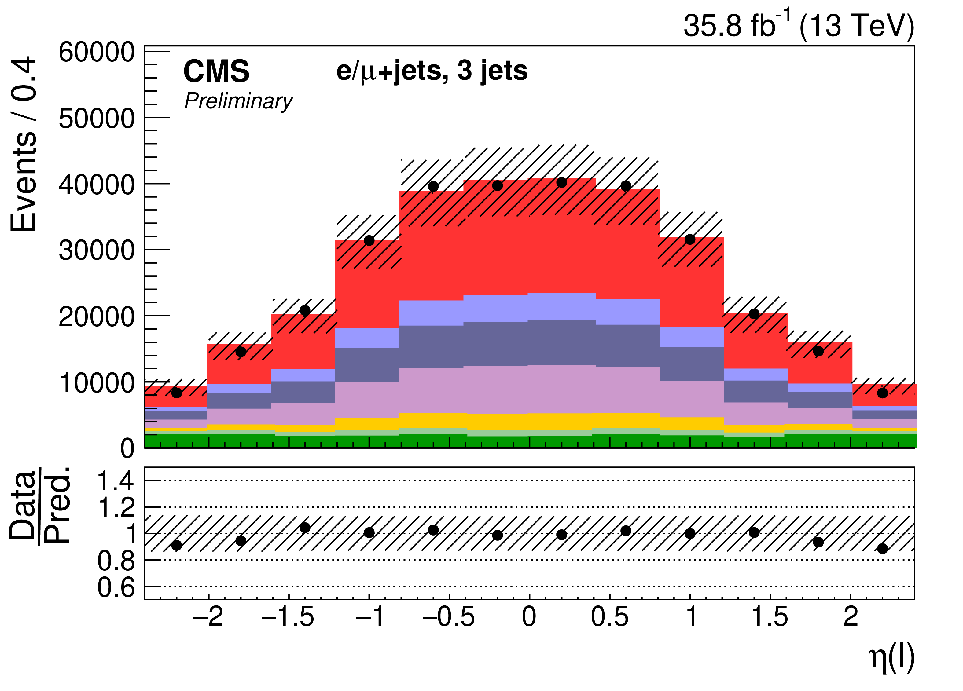
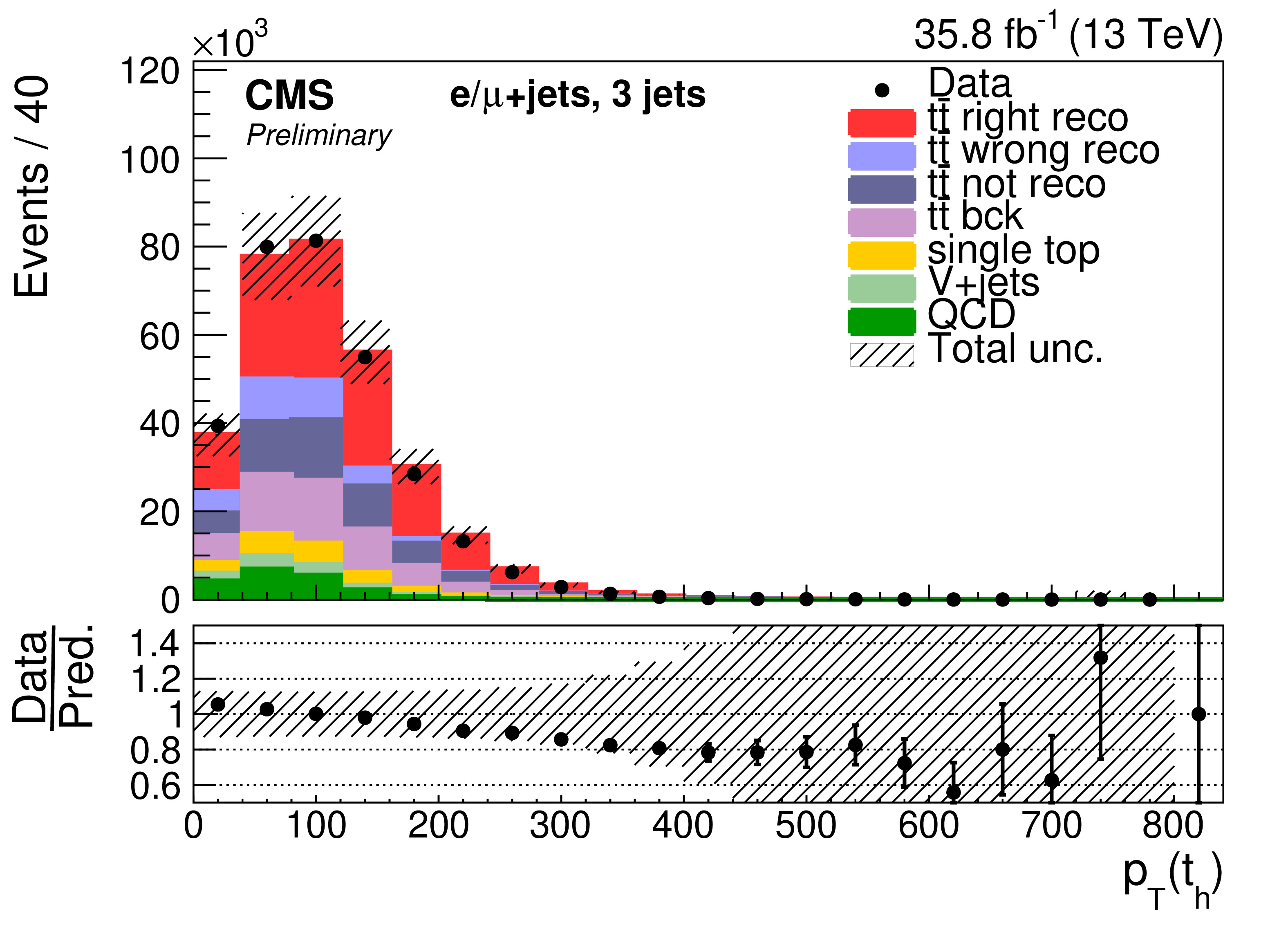
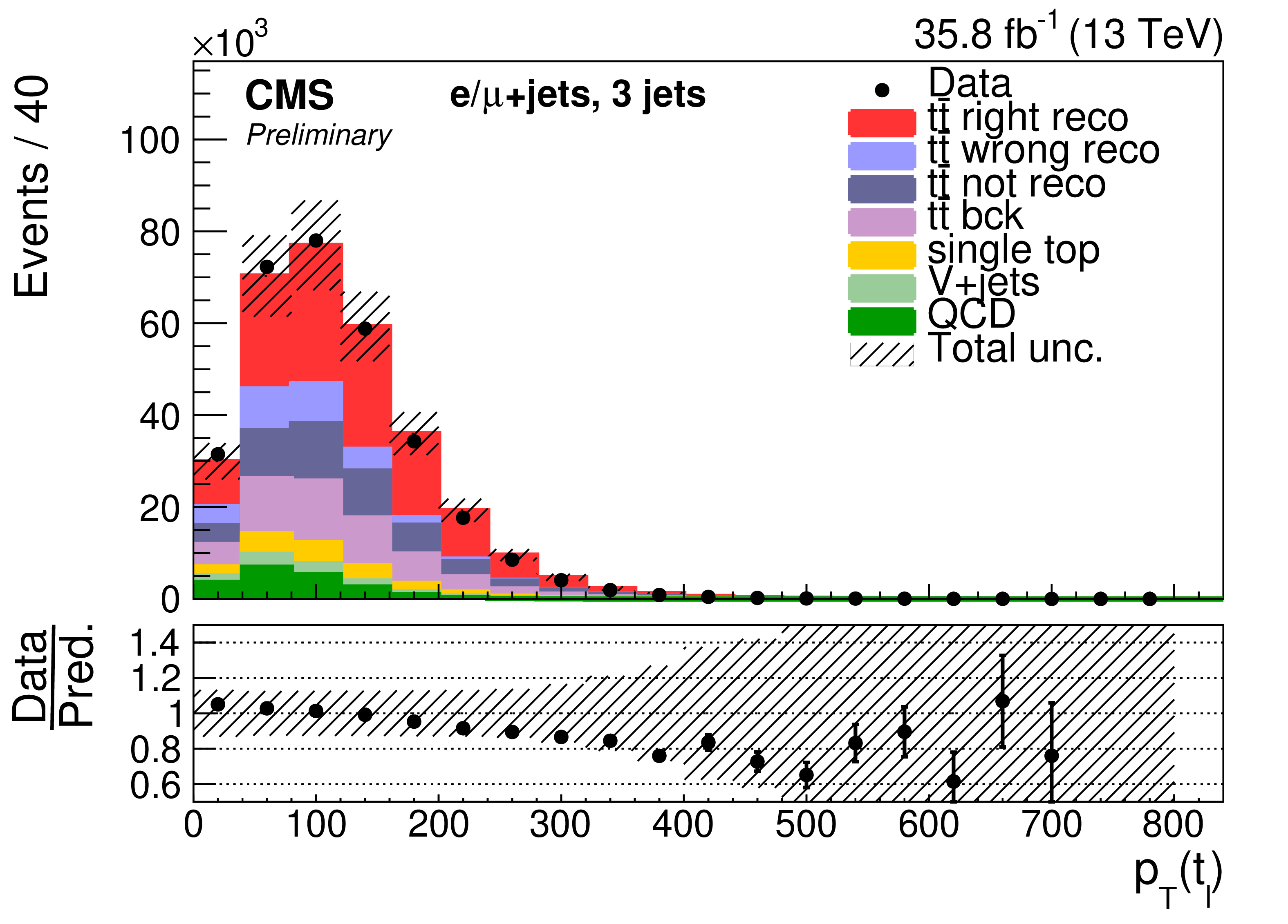
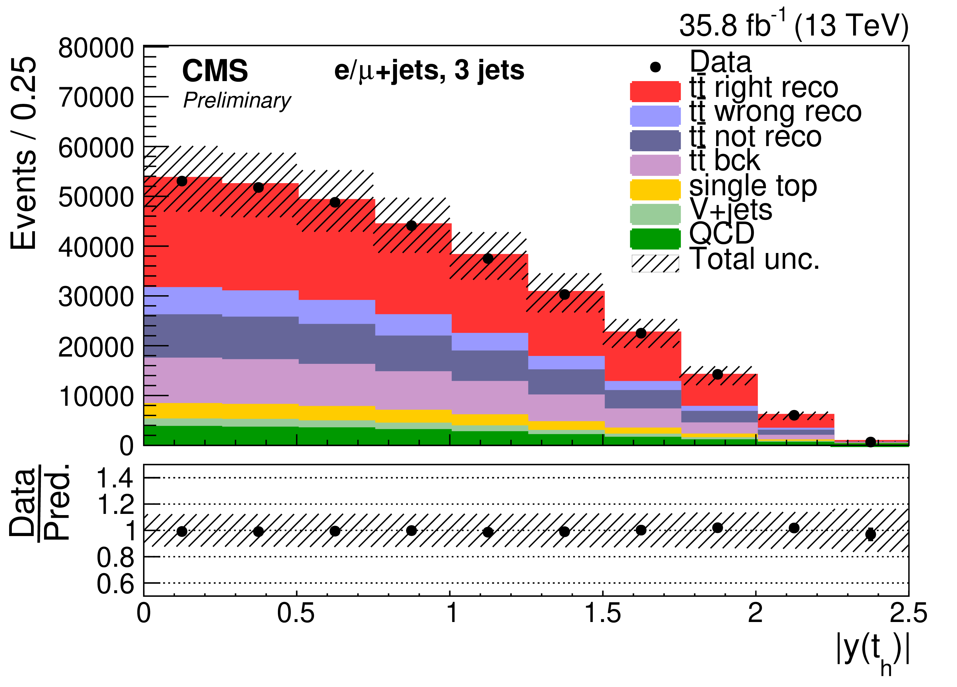
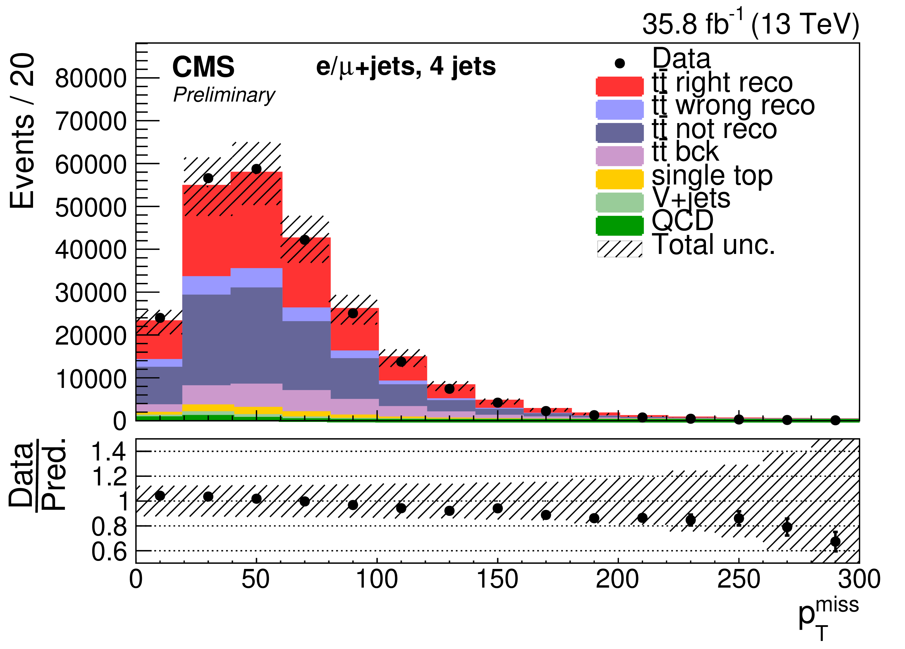
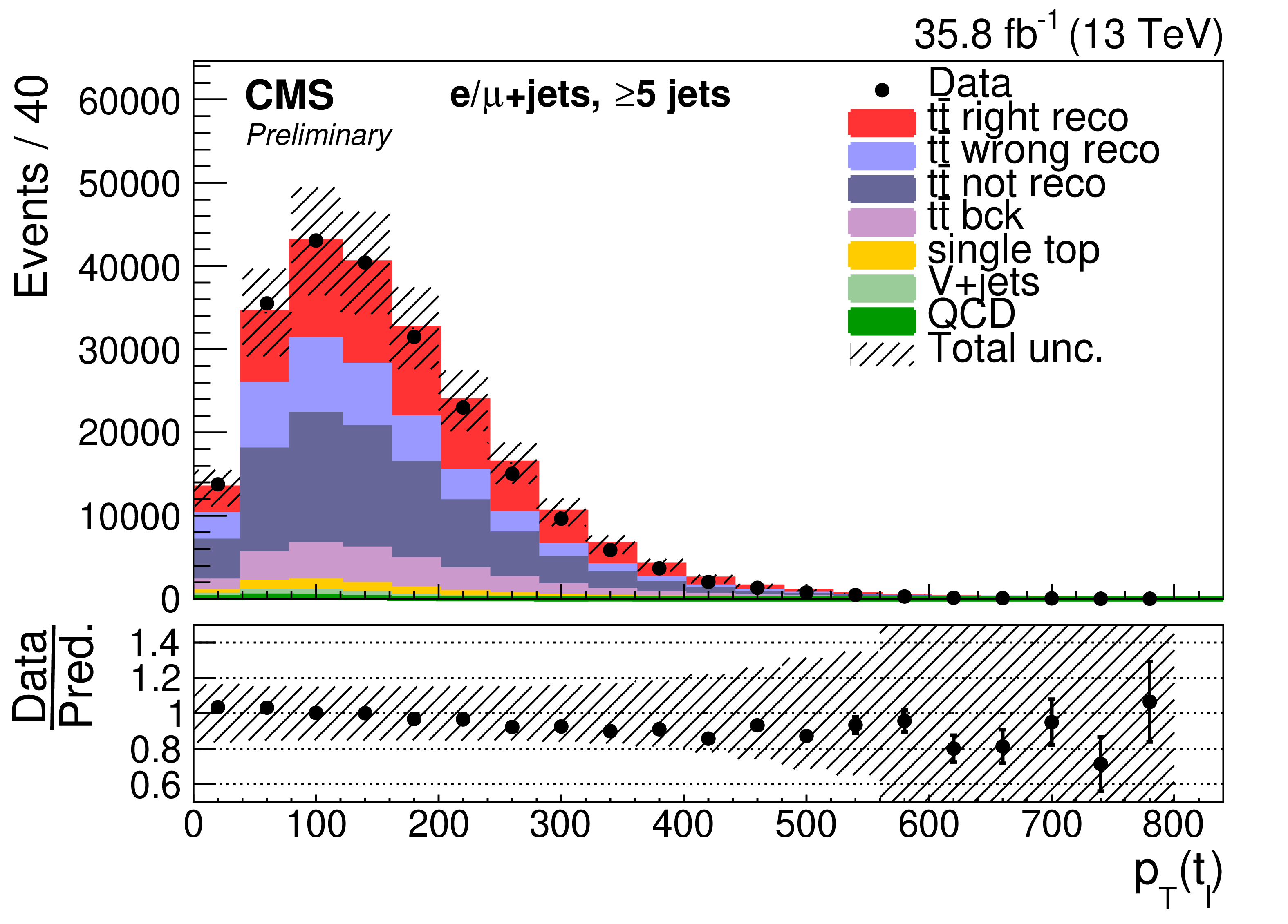
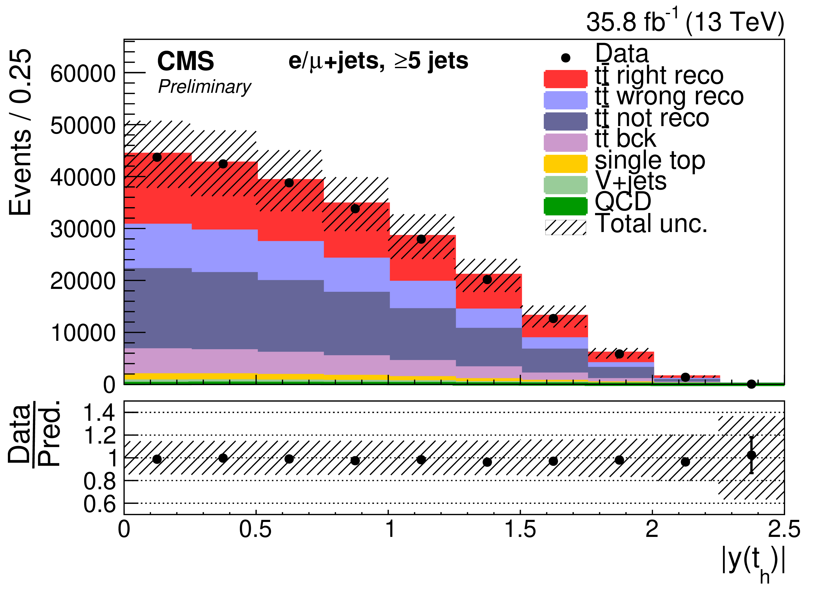
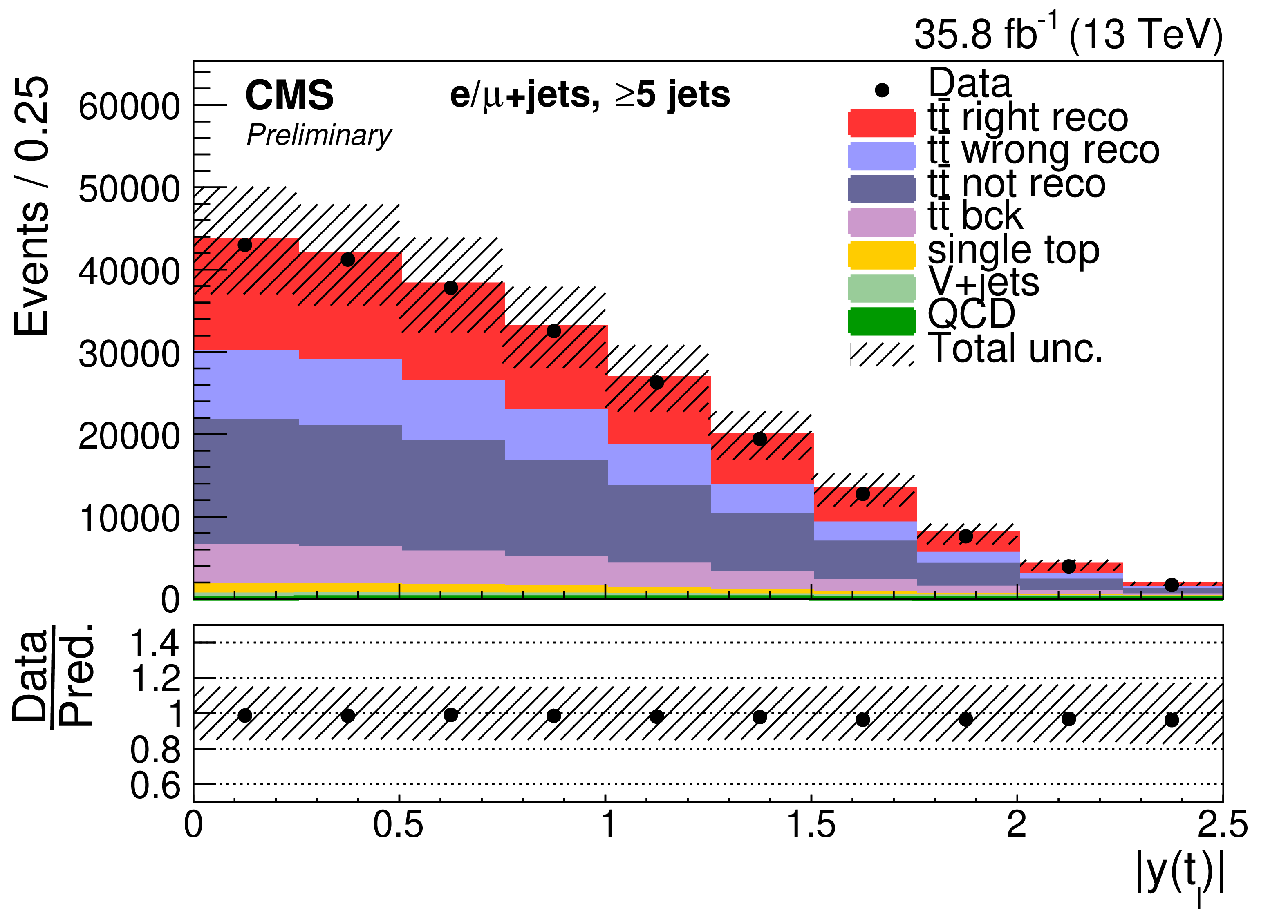
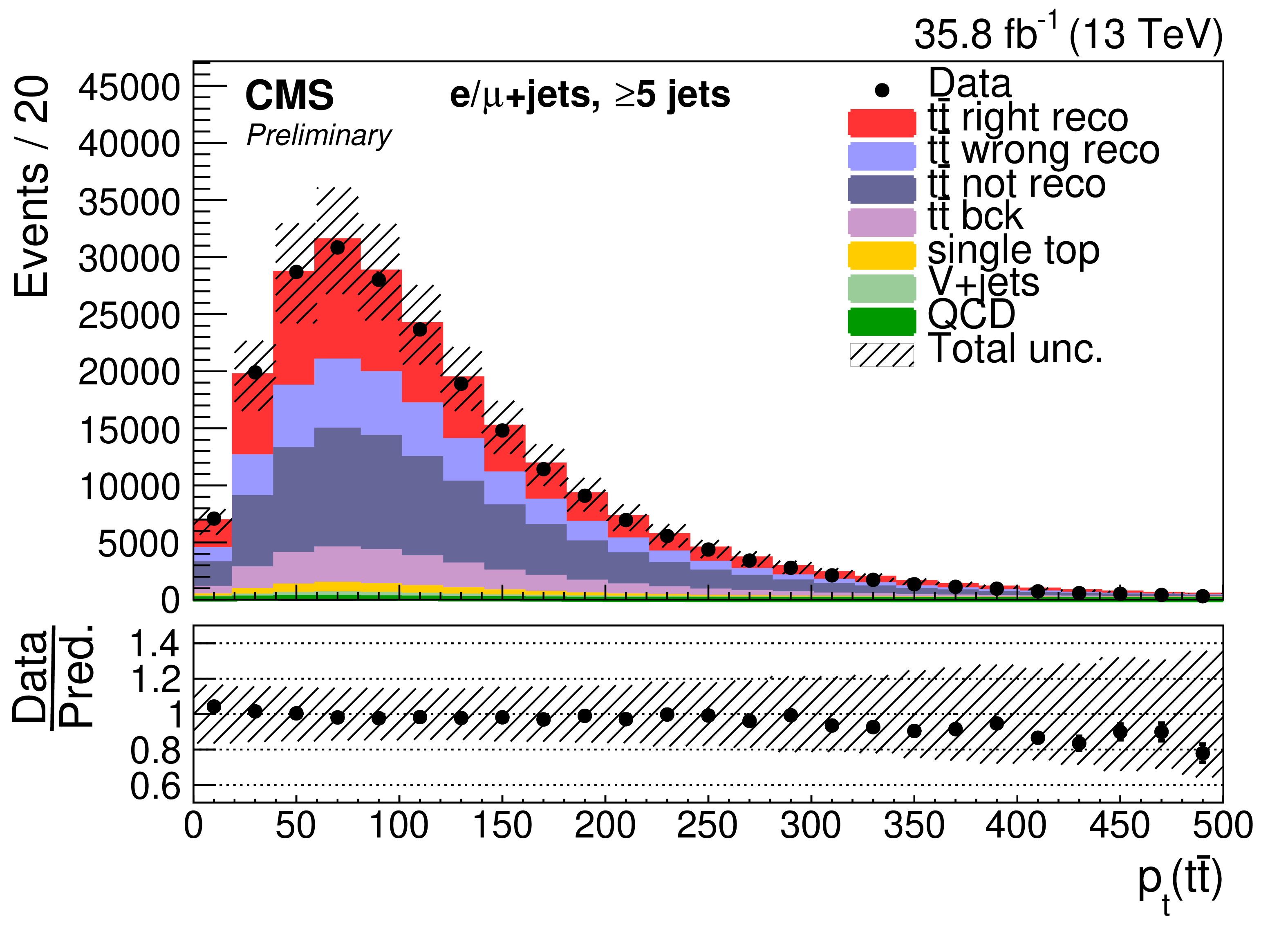
Three-jet events after selection and $ {{\mathrm {t}\overline {\mathrm {t}}}} $ reconstruction. The plots show the missing transverse momentum ($ {p_\mathrm {T}^{\mathrm {miss}}}$), the lepton pseudorapidity, and $ {p_{\mathrm {T}}} $ and absolute rapidity $y$ of leptonic top quark, hadronic top quark, and the $ {{\mathrm {t}\overline {\mathrm {t}}}} $ system. The hatched band shows the total uncertainty associated with signal and background predictions with the sources of uncertainty uncorrelated and summed in quadrature. The ratios of data to the sum of the predicted yields are provided at the bottom of each panel. |
png pdf |
Figure 5-a:
Three-jet events after selection and $ {{\mathrm {t}\overline {\mathrm {t}}}} $ reconstruction. The plot shows the missing transverse momentum ($ {p_\mathrm {T}^{\mathrm {miss}}}$). The hatched band shows the total uncertainty associated with signal and background predictions with the sources of uncertainty uncorrelated and summed in quadrature. The ratios of data to the sum of the predicted yields are provided at the bottom of the panel. |
png pdf |
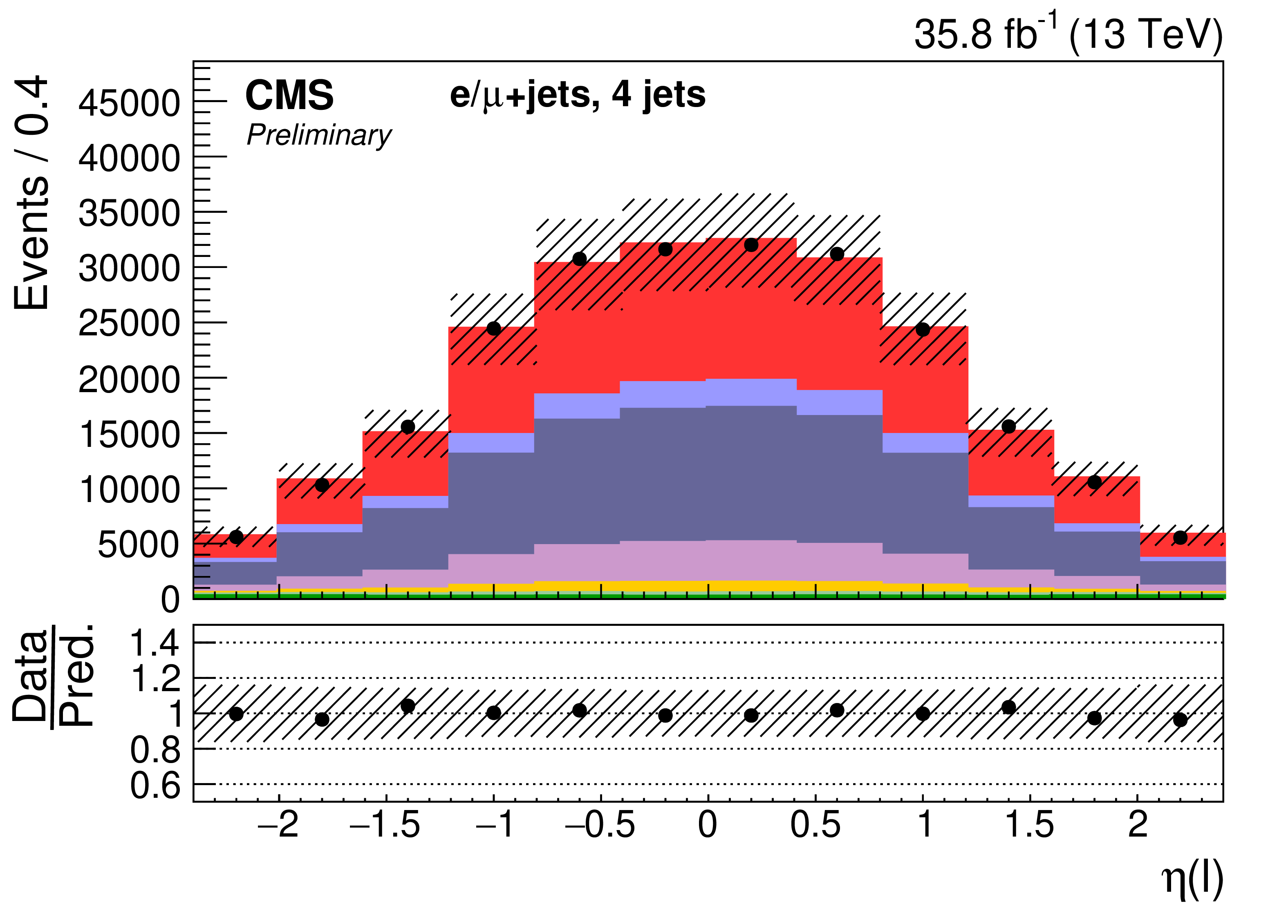
Figure 5-b:
Three-jet events after selection and $ {{\mathrm {t}\overline {\mathrm {t}}}} $ reconstruction. The plot shows the lepton pseudorapidity. The hatched band shows the total uncertainty associated with signal and background predictions with the sources of uncertainty uncorrelated and summed in quadrature. The ratios of data to the sum of the predicted yields are provided at the bottom of the panel. |
png pdf |
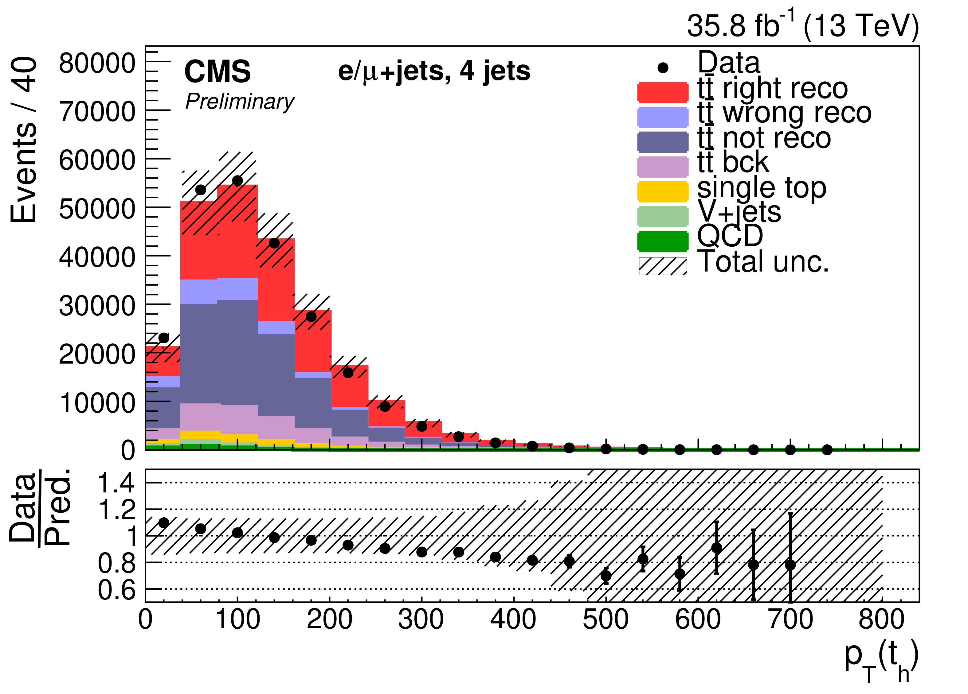
Figure 5-c:
Three-jet events after selection and $ {{\mathrm {t}\overline {\mathrm {t}}}} $ reconstruction. The plot shows the $ {p_{\mathrm {T}}} $ of the hadronic top quark. The hatched band shows the total uncertainty associated with signal and background predictions with the sources of uncertainty uncorrelated and summed in quadrature. The ratios of data to the sum of the predicted yields are provided at the bottom of the panel. |
png pdf |
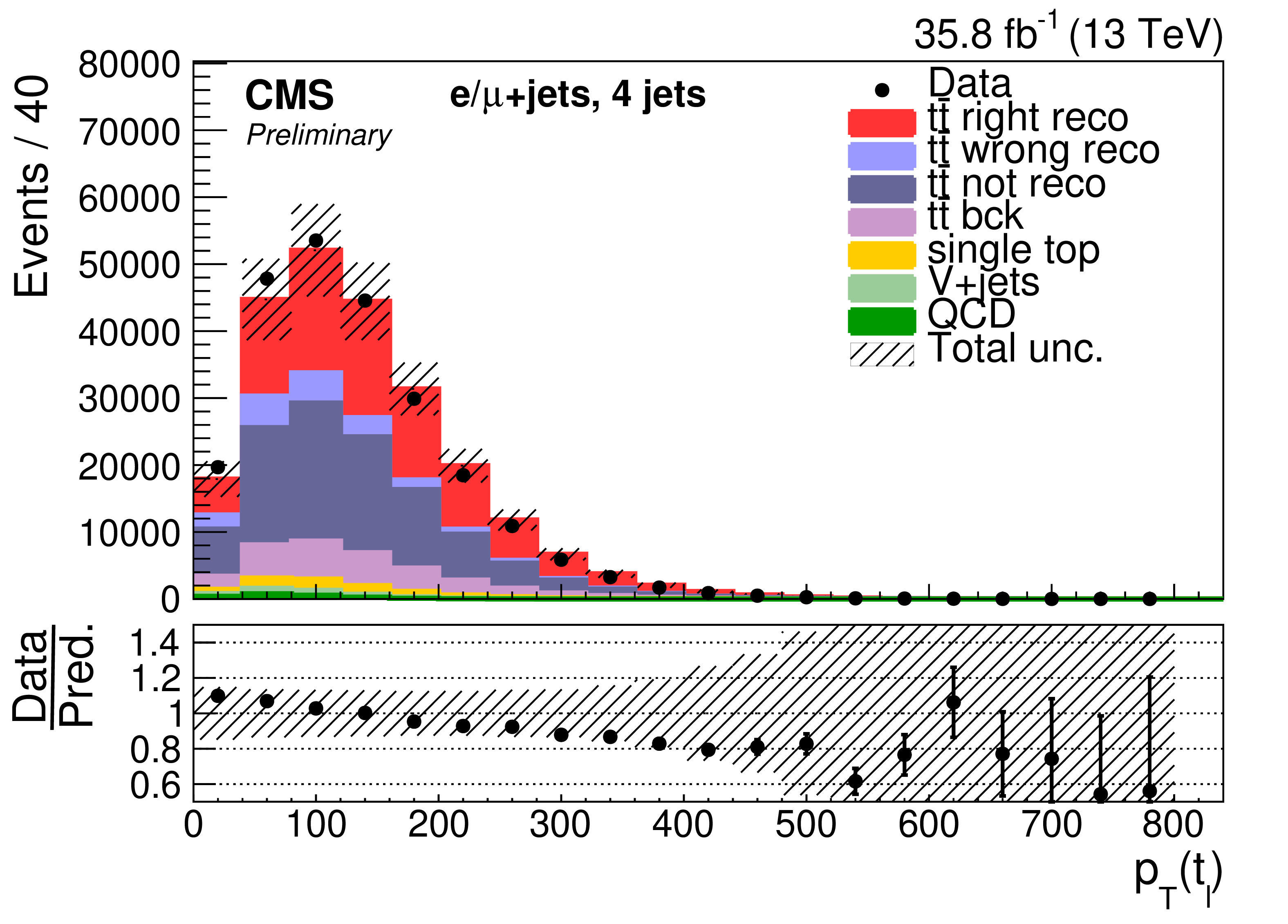
Figure 5-d:
Three-jet events after selection and $ {{\mathrm {t}\overline {\mathrm {t}}}} $ reconstruction. The plot shows the $ {p_{\mathrm {T}}} $ of the leptonic top quark. The hatched band shows the total uncertainty associated with signal and background predictions with the sources of uncertainty uncorrelated and summed in quadrature. The ratios of data to the sum of the predicted yields are provided at the bottom of the panel. |
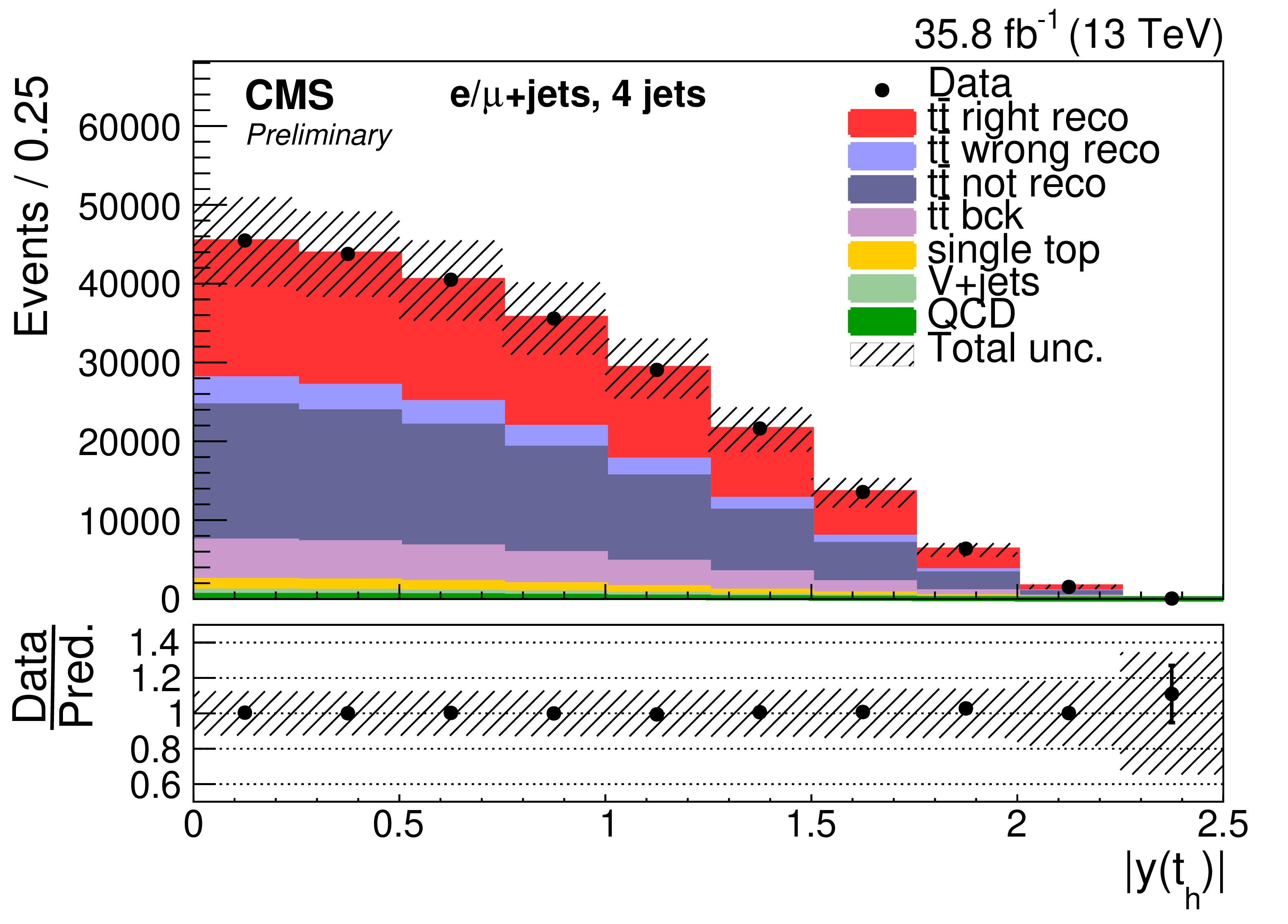
png pdf |
Figure 5-e:
Three-jet events after selection and $ {{\mathrm {t}\overline {\mathrm {t}}}} $ reconstruction. The plot shows the absolute rapidity $y$ of the hadronic top quark. The hatched band shows the total uncertainty associated with signal and background predictions with the sources of uncertainty uncorrelated and summed in quadrature. The ratios of data to the sum of the predicted yields are provided at the bottom of the panel. |
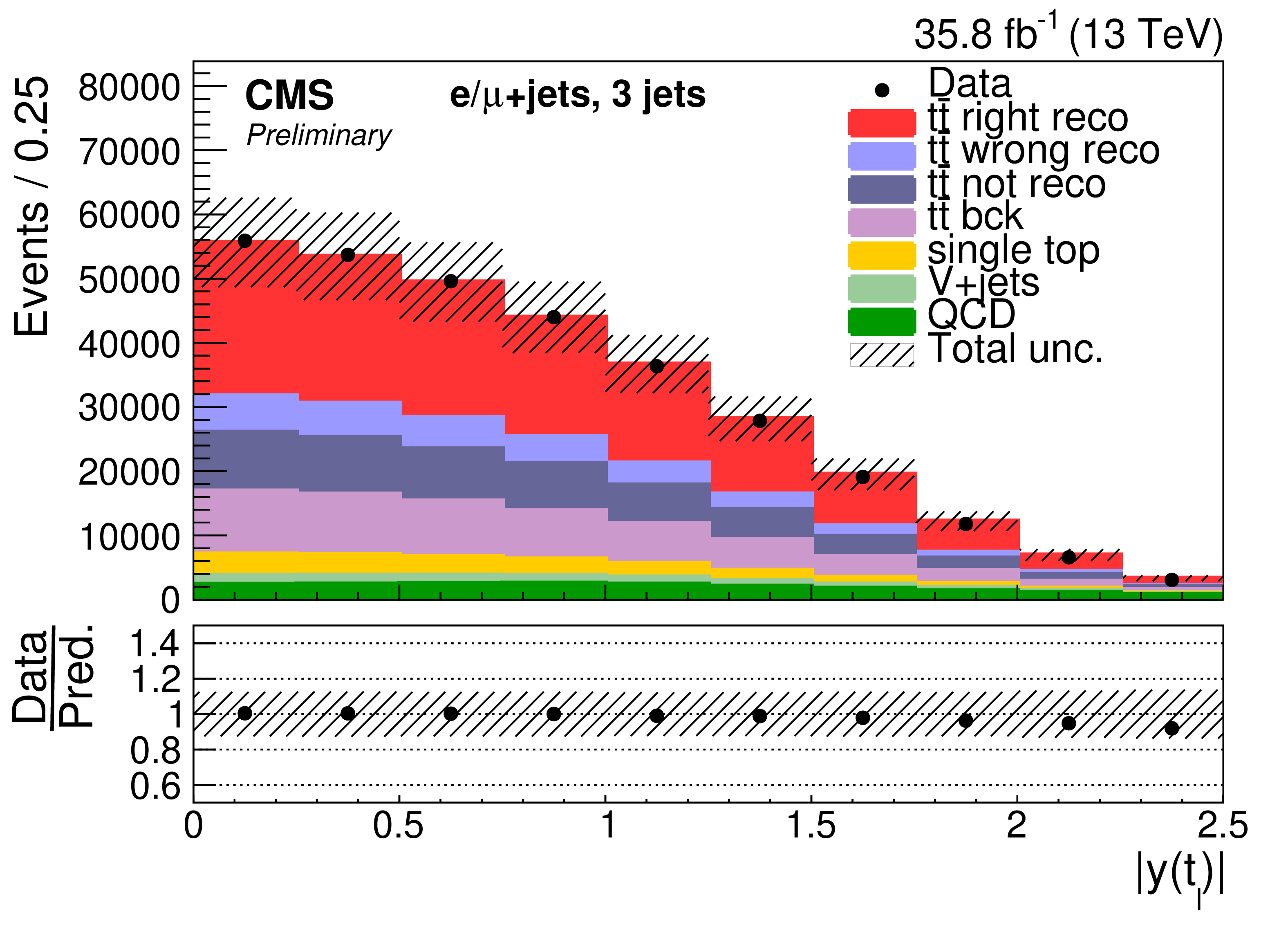
png pdf |
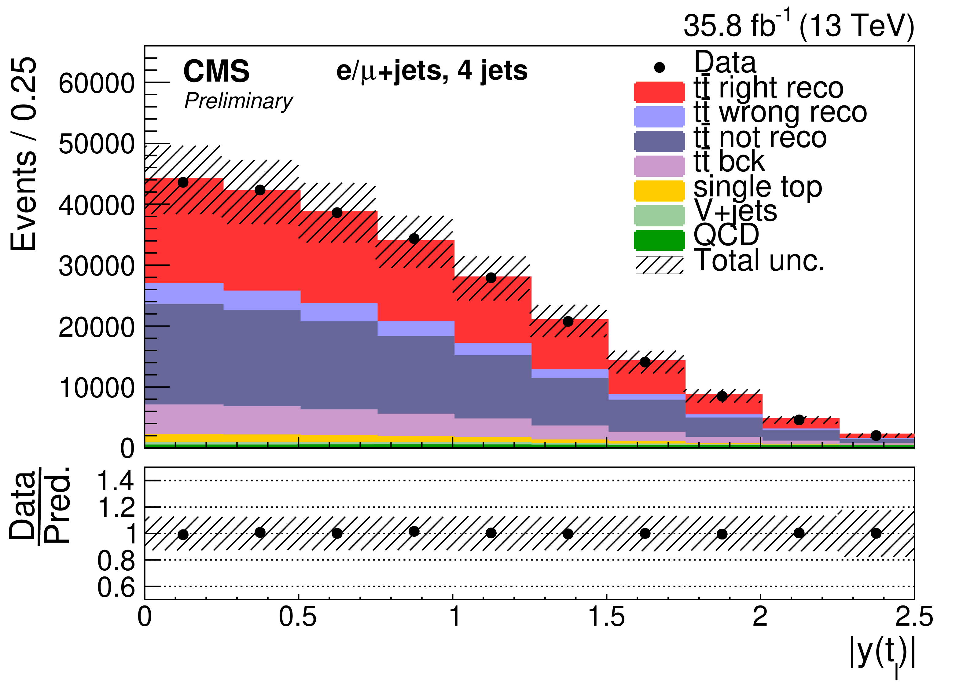
Figure 5-f:
Three-jet events after selection and $ {{\mathrm {t}\overline {\mathrm {t}}}} $ reconstruction. The plot shows the absolute rapidity $y$ of the leptonic top quark. The hatched band shows the total uncertainty associated with signal and background predictions with the sources of uncertainty uncorrelated and summed in quadrature. The ratios of data to the sum of the predicted yields are provided at the bottom of the panel. |
png pdf |
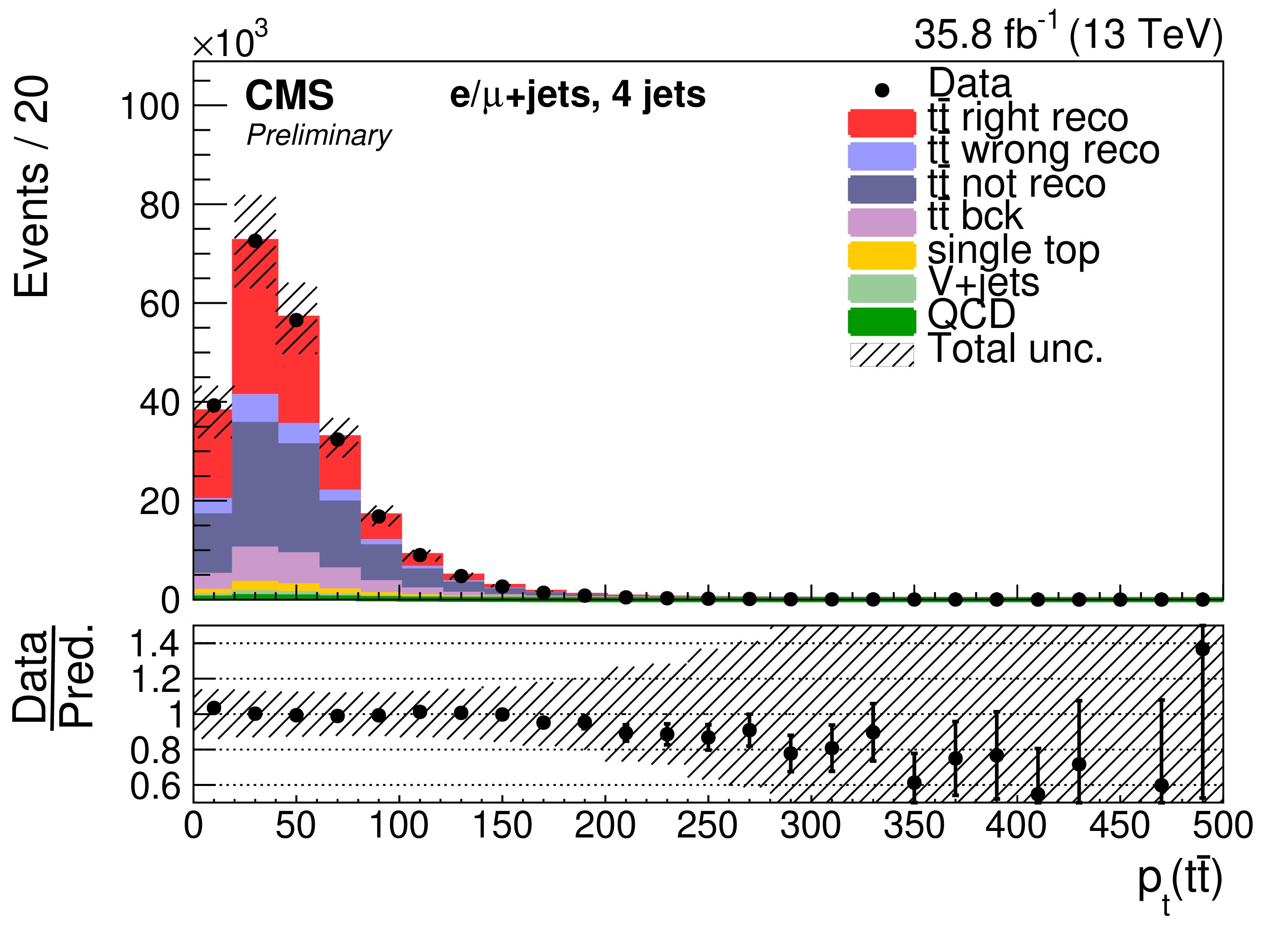
Figure 5-g:
Three-jet events after selection and $ {{\mathrm {t}\overline {\mathrm {t}}}} $ reconstruction. The plot shows the $ {p_{\mathrm {T}}} $ of the $ {{\mathrm {t}\overline {\mathrm {t}}}} $ system. The hatched band shows the total uncertainty associated with signal and background predictions with the sources of uncertainty uncorrelated and summed in quadrature. The ratios of data to the sum of the predicted yields are provided at the bottom of the panel. |
png pdf |
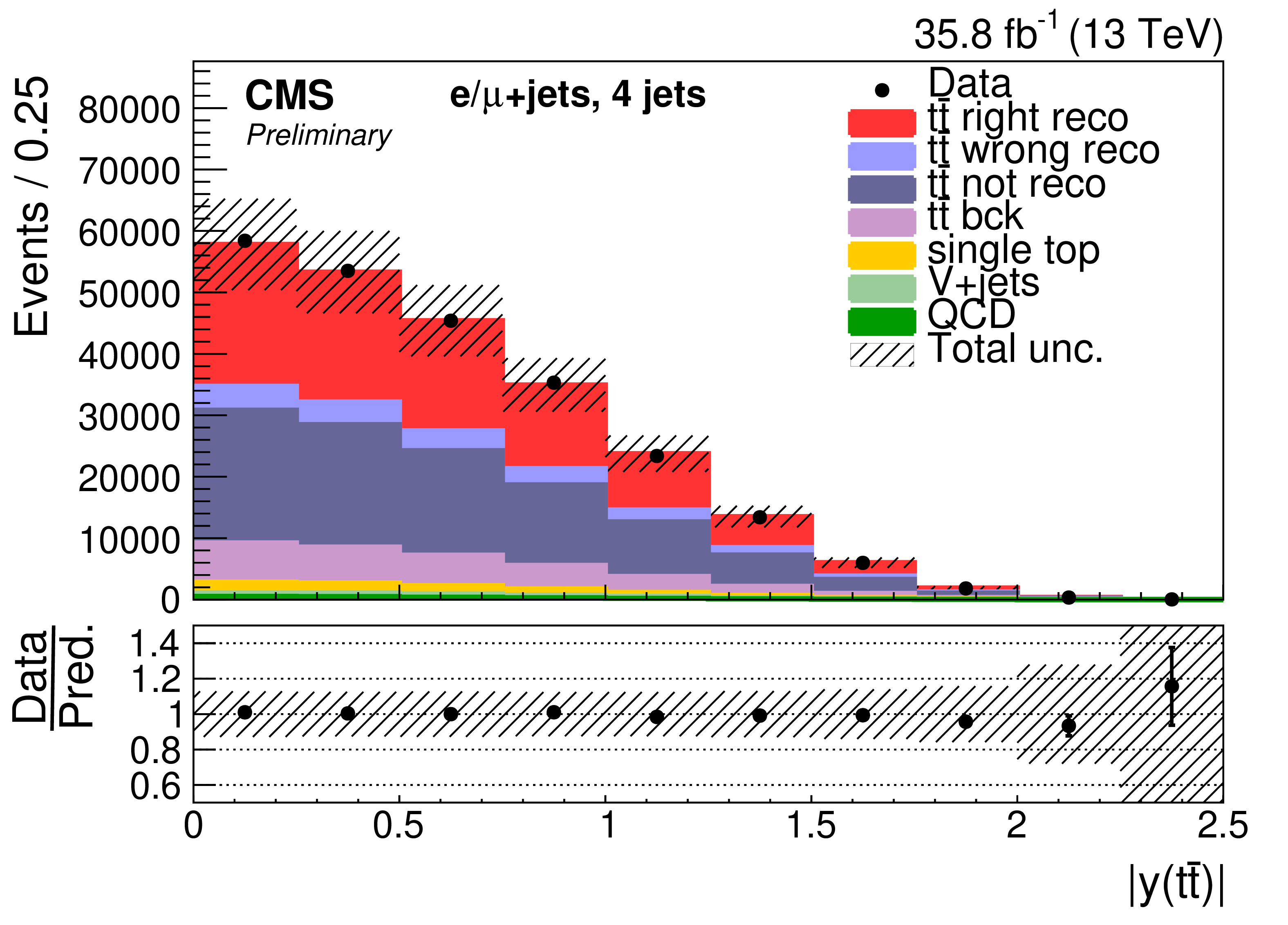
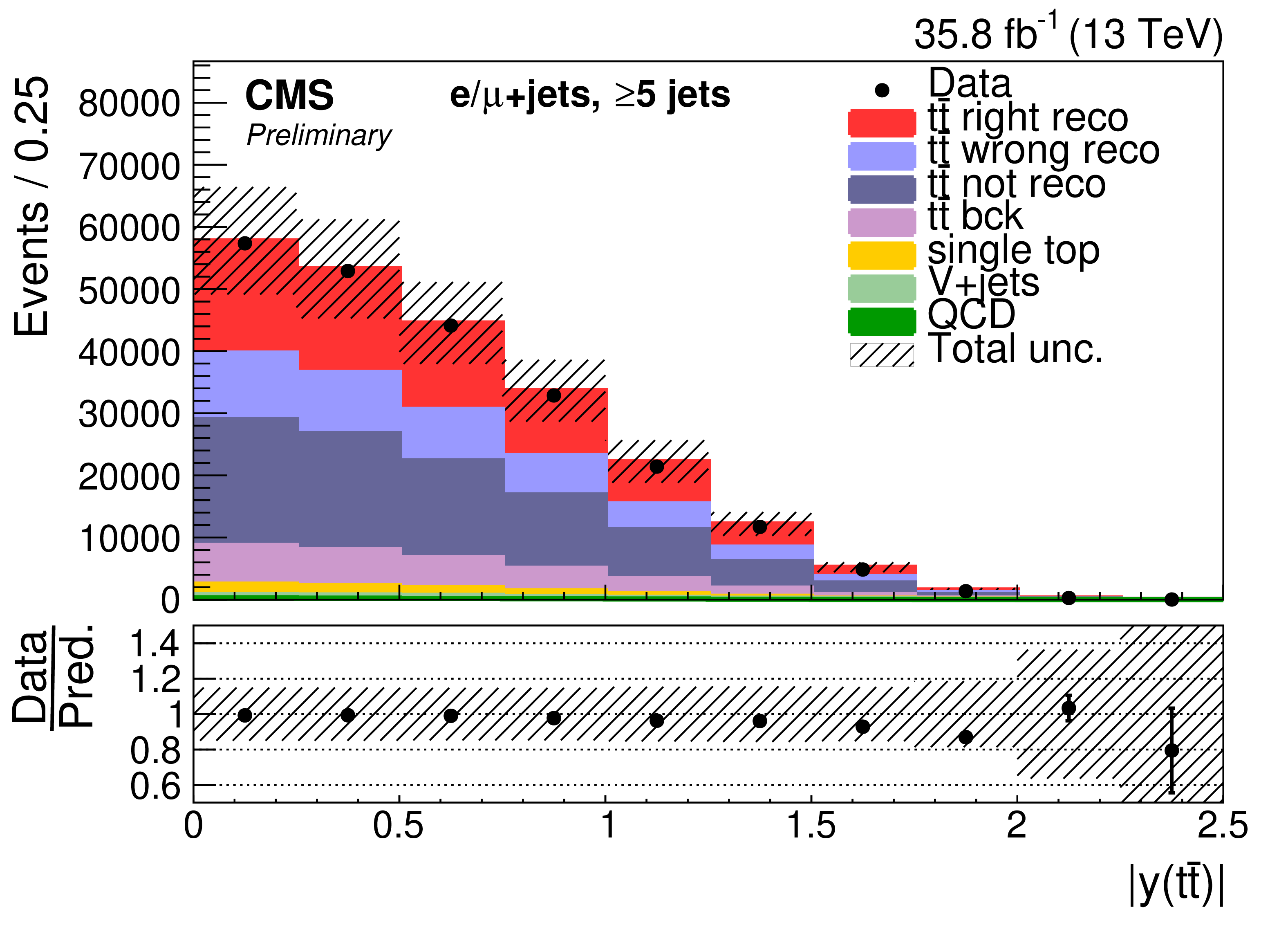
Figure 5-h:
Three-jet events after selection and $ {{\mathrm {t}\overline {\mathrm {t}}}} $ reconstruction. The plot shows the absolute rapidity $y$ of the $ {{\mathrm {t}\overline {\mathrm {t}}}} $ system. The hatched band shows the total uncertainty associated with signal and background predictions with the sources of uncertainty uncorrelated and summed in quadrature. The ratios of data to the sum of the predicted yields are provided at the bottom of the panel. |
png pdf |
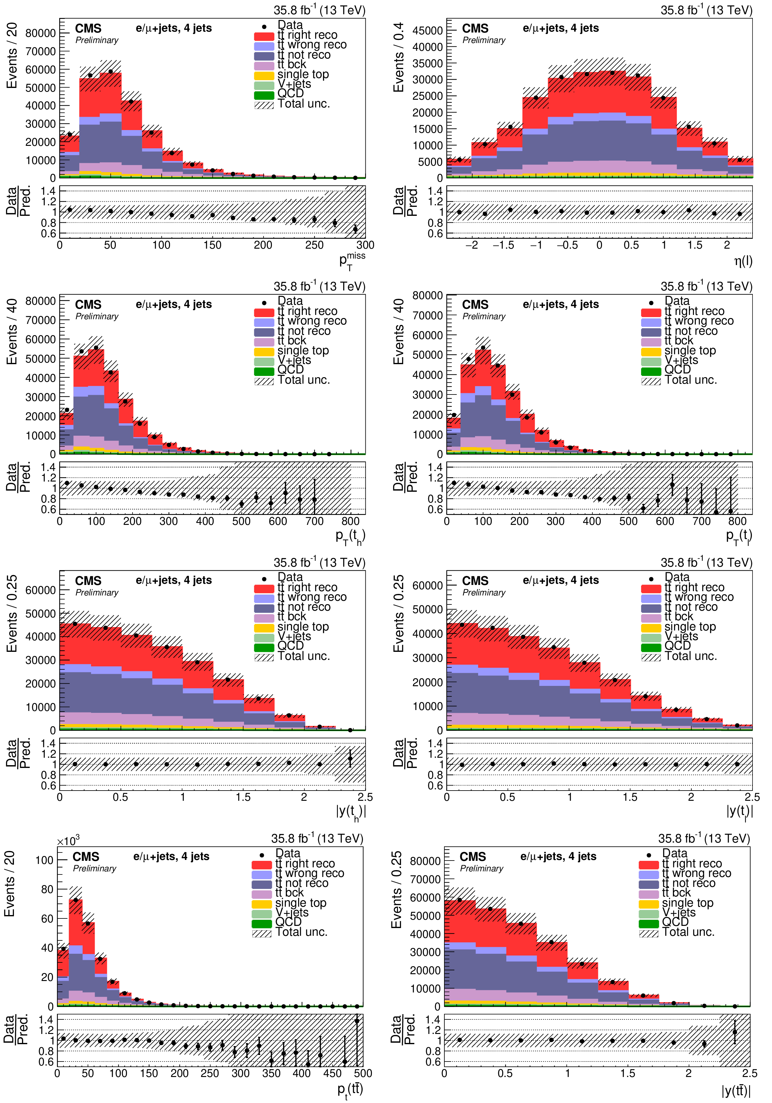
Figure 6:
Four-jet events after selection and $ {{\mathrm {t}\overline {\mathrm {t}}}} $ reconstruction. Same plots as described in Fig. 5. |
png pdf |
Figure 6-a:
Four-jet events after selection and $ {{\mathrm {t}\overline {\mathrm {t}}}} $ reconstruction. Same as corresponding plot in Fig. 5. |
png pdf |
Figure 6-b:
Four-jet events after selection and $ {{\mathrm {t}\overline {\mathrm {t}}}} $ reconstruction. Same as corresponding plot in Fig. 5. |
png pdf |
Figure 6-c:
Four-jet events after selection and $ {{\mathrm {t}\overline {\mathrm {t}}}} $ reconstruction. Same as corresponding plot in Fig. 5. |
png pdf |
Figure 6-d:
Four-jet events after selection and $ {{\mathrm {t}\overline {\mathrm {t}}}} $ reconstruction. Same as corresponding plot in Fig. 5. |
png pdf |
Figure 6-e:
Four-jet events after selection and $ {{\mathrm {t}\overline {\mathrm {t}}}} $ reconstruction. Same as corresponding plot in Fig. 5. |
png pdf |
Figure 6-f:
Four-jet events after selection and $ {{\mathrm {t}\overline {\mathrm {t}}}} $ reconstruction. Same as corresponding plot in Fig. 5. |
png pdf |
Figure 6-g:
Four-jet events after selection and $ {{\mathrm {t}\overline {\mathrm {t}}}} $ reconstruction. Same as corresponding plot in Fig. 5. |
png pdf |
Figure 6-h:
Four-jet events after selection and $ {{\mathrm {t}\overline {\mathrm {t}}}} $ reconstruction. Same as corresponding plot in Fig. 5. |
png pdf |
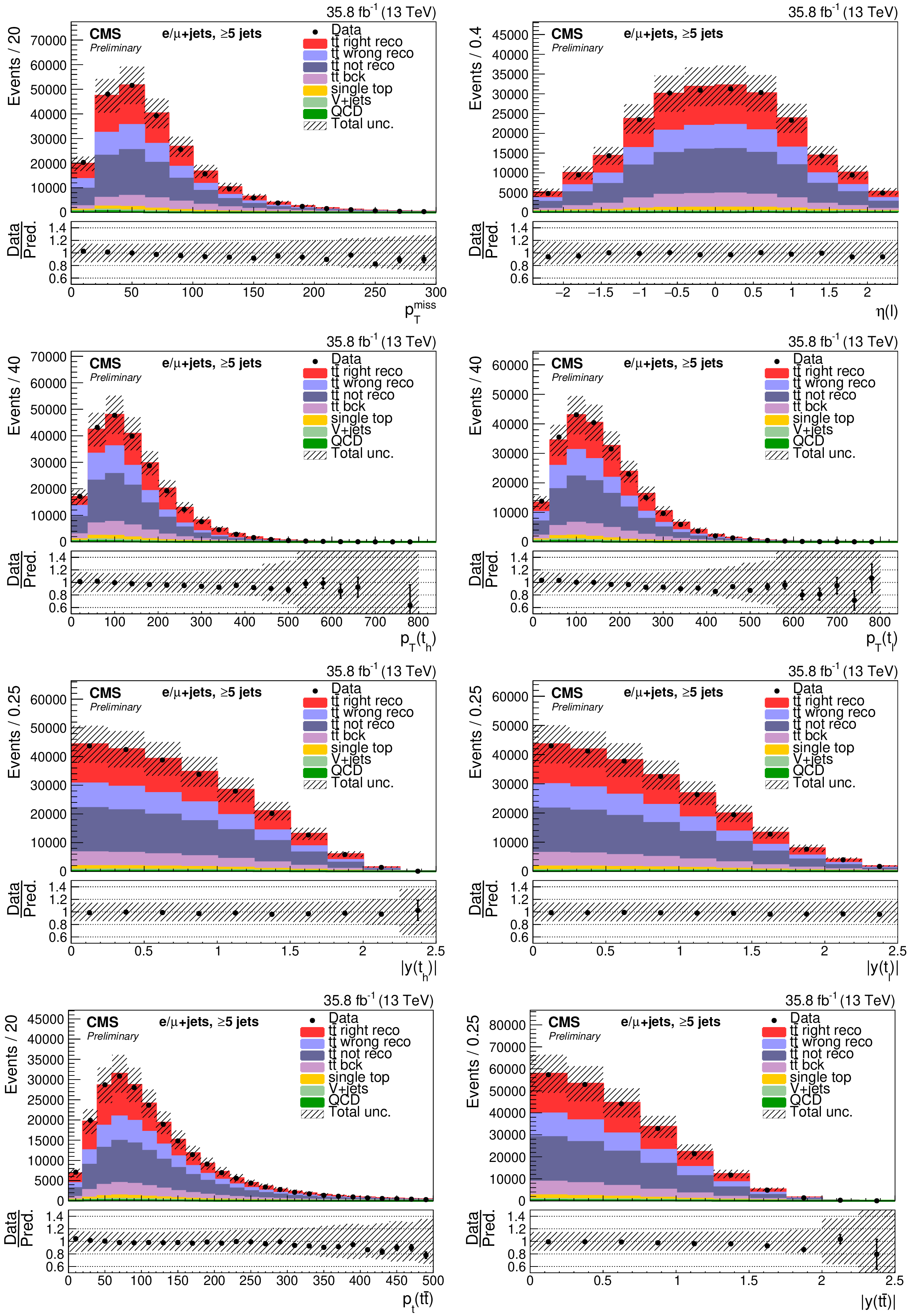
Figure 7:
Events with five or more jets after selection and $ {{\mathrm {t}\overline {\mathrm {t}}}} $ reconstruction. Same plots as described in Fig. 5. |
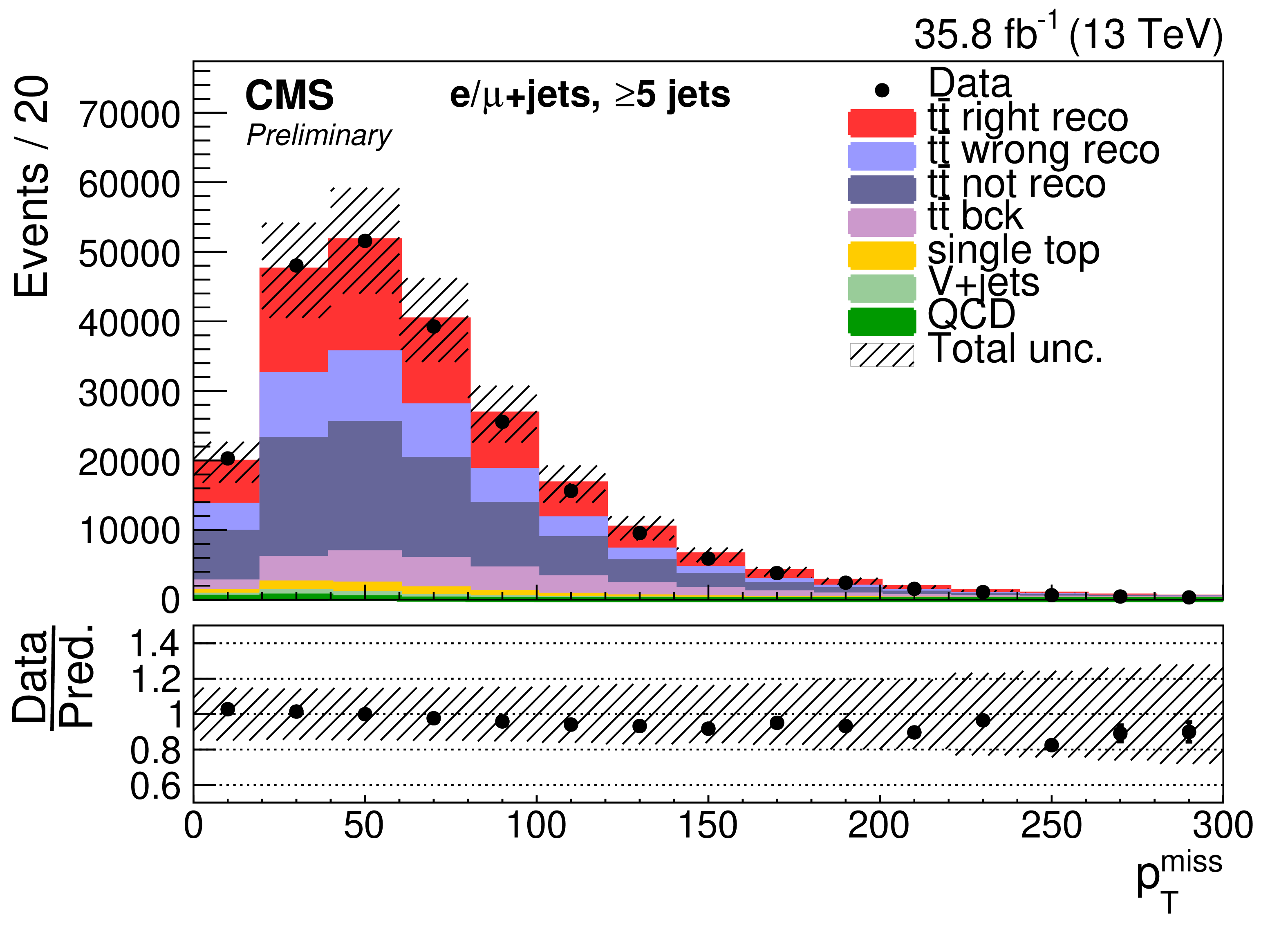
png pdf |
Figure 7-a:
Events with five or more jets after selection and $ {{\mathrm {t}\overline {\mathrm {t}}}} $ reconstruction. Same as corresponding plot in Fig. 5. |
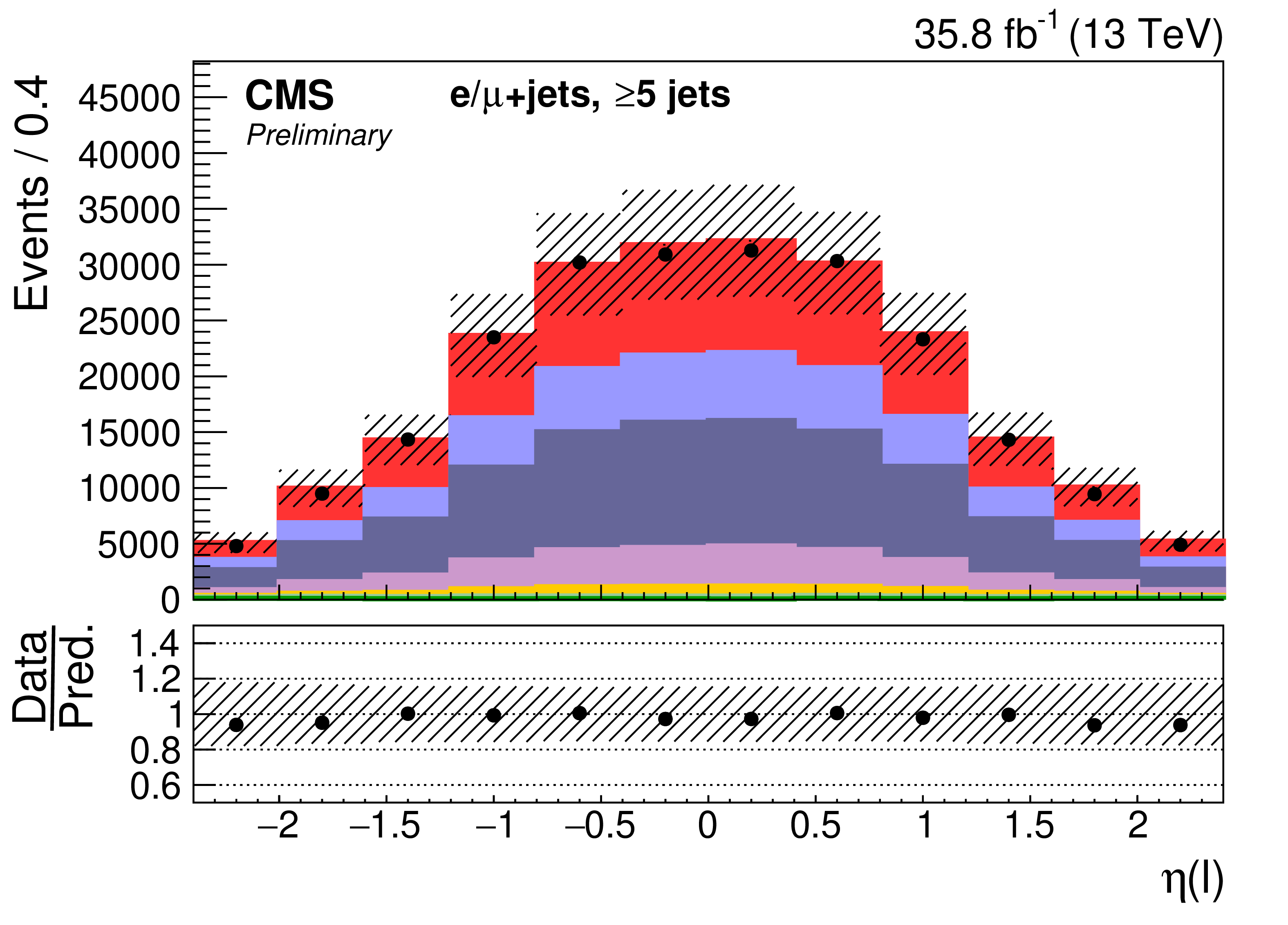
png pdf |
Figure 7-b:
Events with five or more jets after selection and $ {{\mathrm {t}\overline {\mathrm {t}}}} $ reconstruction. Same as corresponding plot in Fig. 5. |
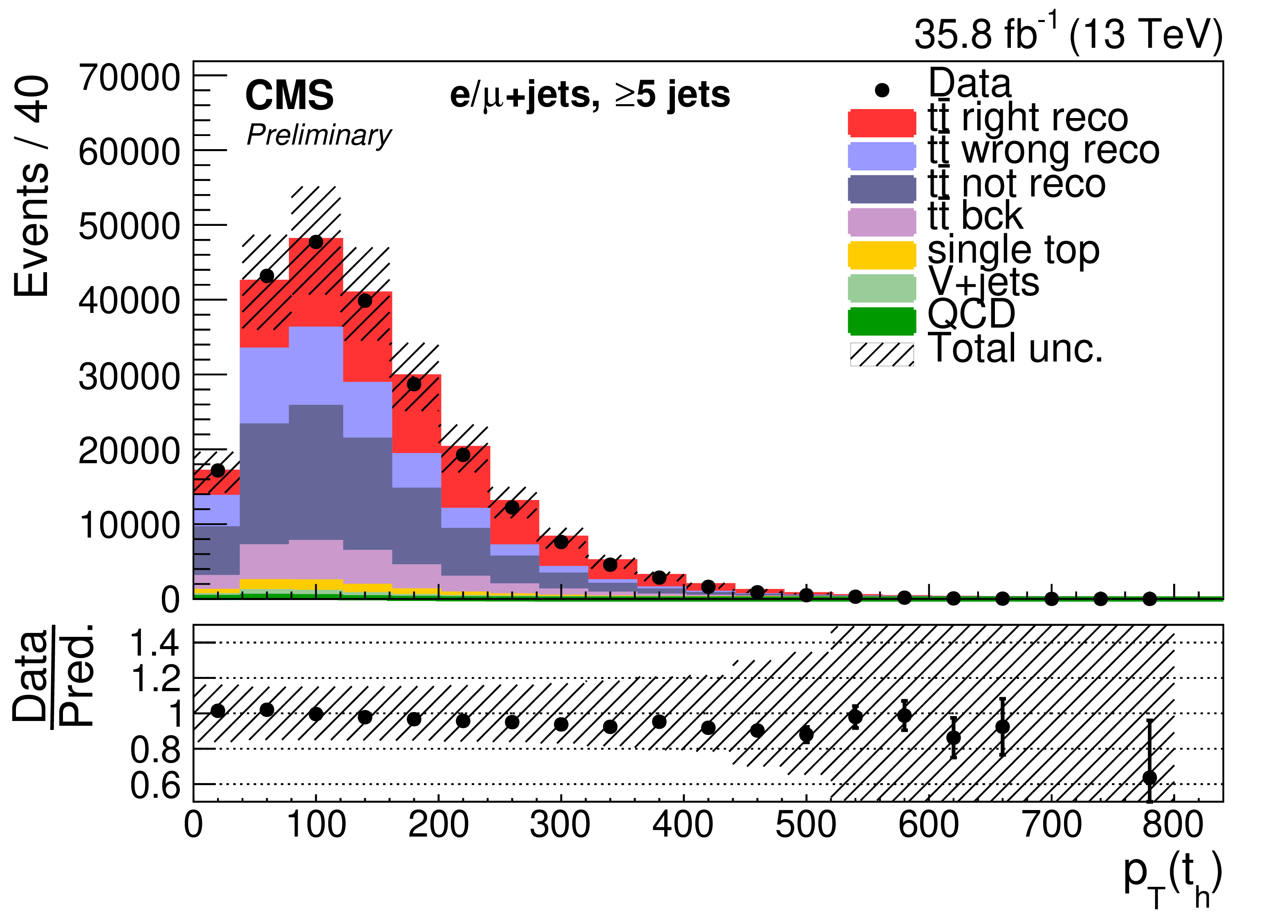
png pdf |
Figure 7-c:
Events with five or more jets after selection and $ {{\mathrm {t}\overline {\mathrm {t}}}} $ reconstruction. Same as corresponding plot in Fig. 5. |
png pdf |
Figure 7-d:
Events with five or more jets after selection and $ {{\mathrm {t}\overline {\mathrm {t}}}} $ reconstruction. Same as corresponding plot in Fig. 5. |
png pdf |
Figure 7-e:
Events with five or more jets after selection and $ {{\mathrm {t}\overline {\mathrm {t}}}} $ reconstruction. Same as corresponding plot in Fig. 5. |
png pdf |
Figure 7-f:
Events with five or more jets after selection and $ {{\mathrm {t}\overline {\mathrm {t}}}} $ reconstruction. Same as corresponding plot in Fig. 5. |
png pdf |
Figure 7-g:
Events with five or more jets after selection and $ {{\mathrm {t}\overline {\mathrm {t}}}} $ reconstruction. Same as corresponding plot in Fig. 5. |
png pdf |
Figure 7-h:
Events with five or more jets after selection and $ {{\mathrm {t}\overline {\mathrm {t}}}} $ reconstruction. Same as corresponding plot in Fig. 5. |
png pdf |
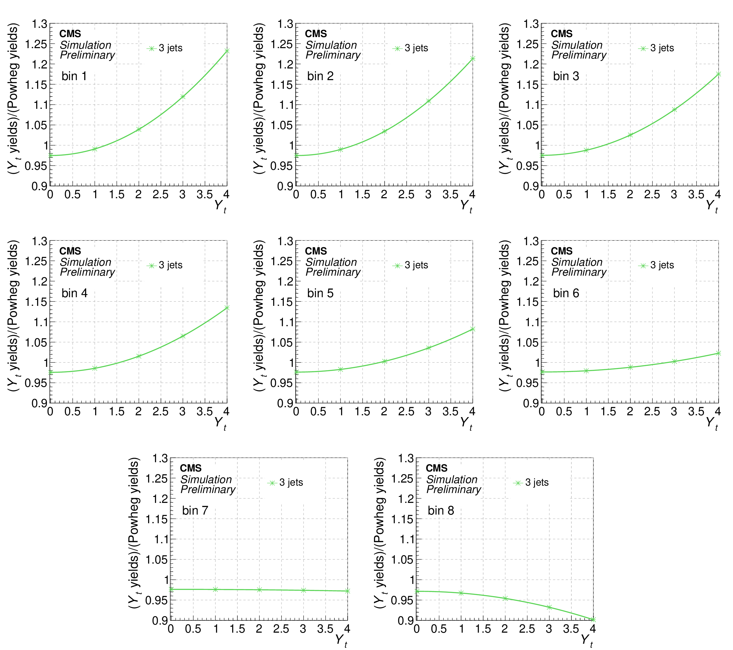
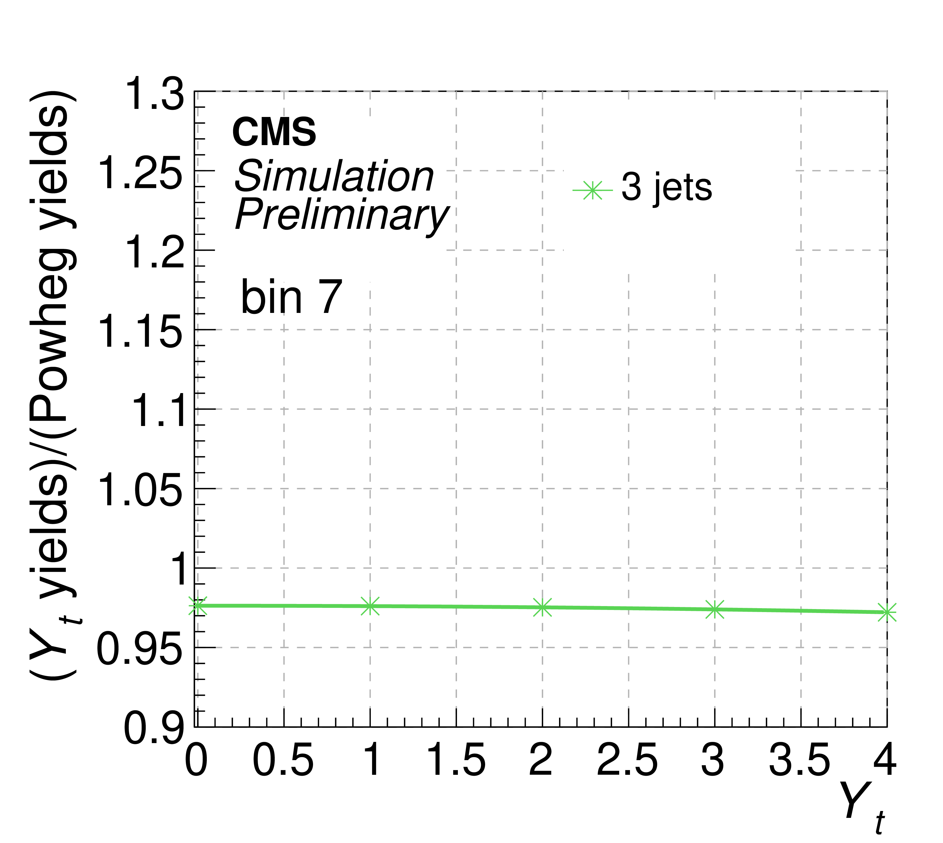
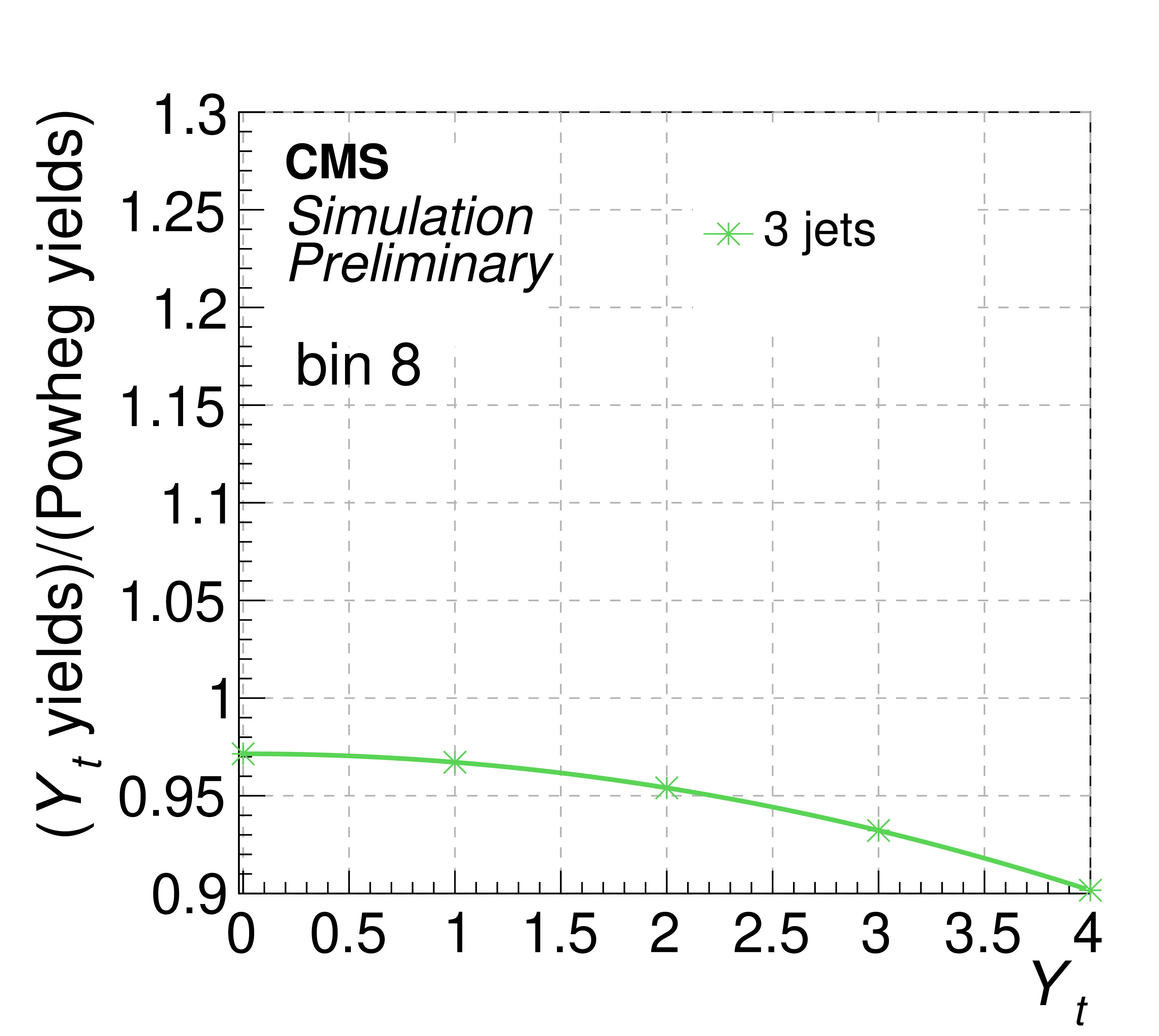
Figure 8:
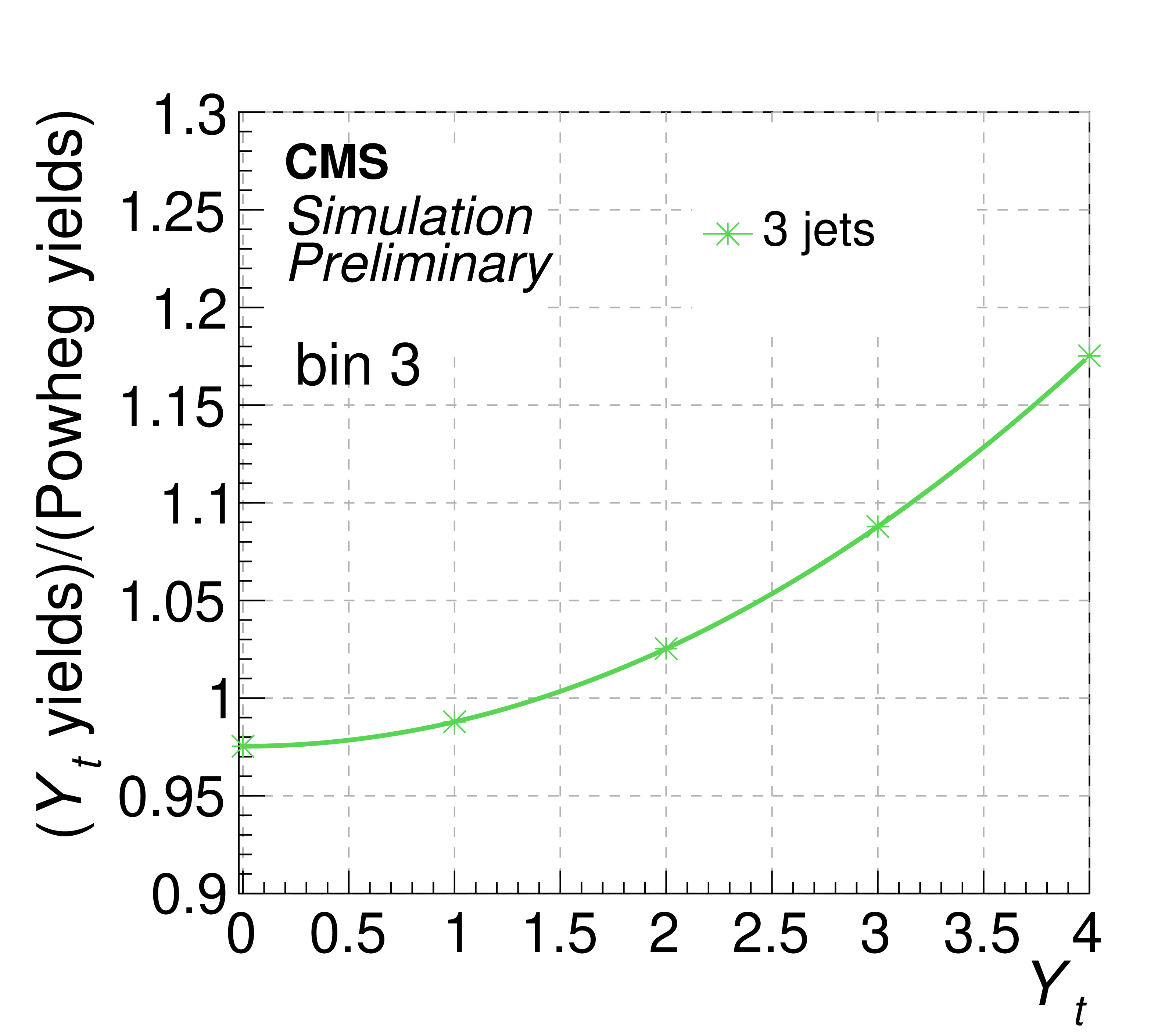
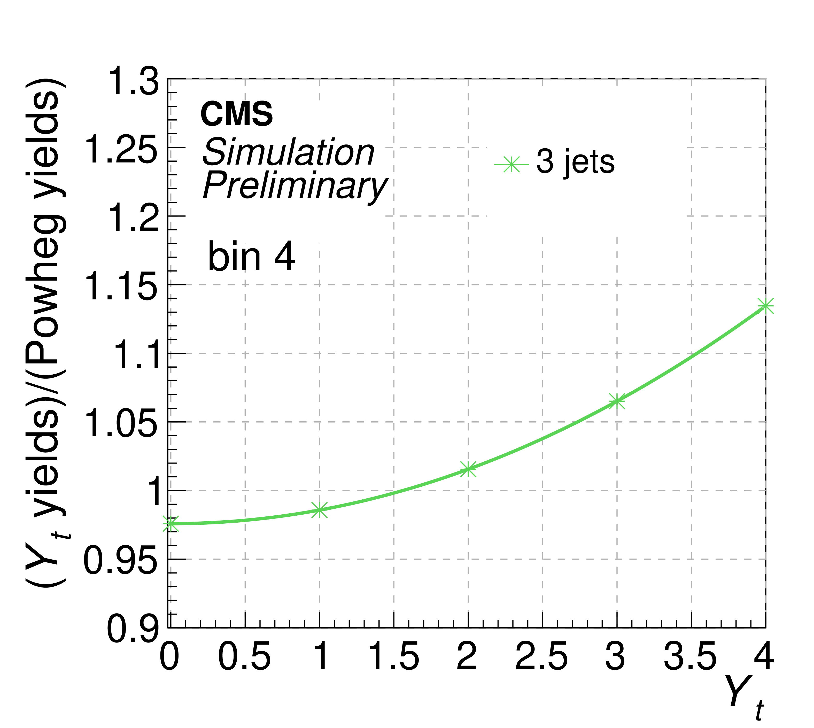
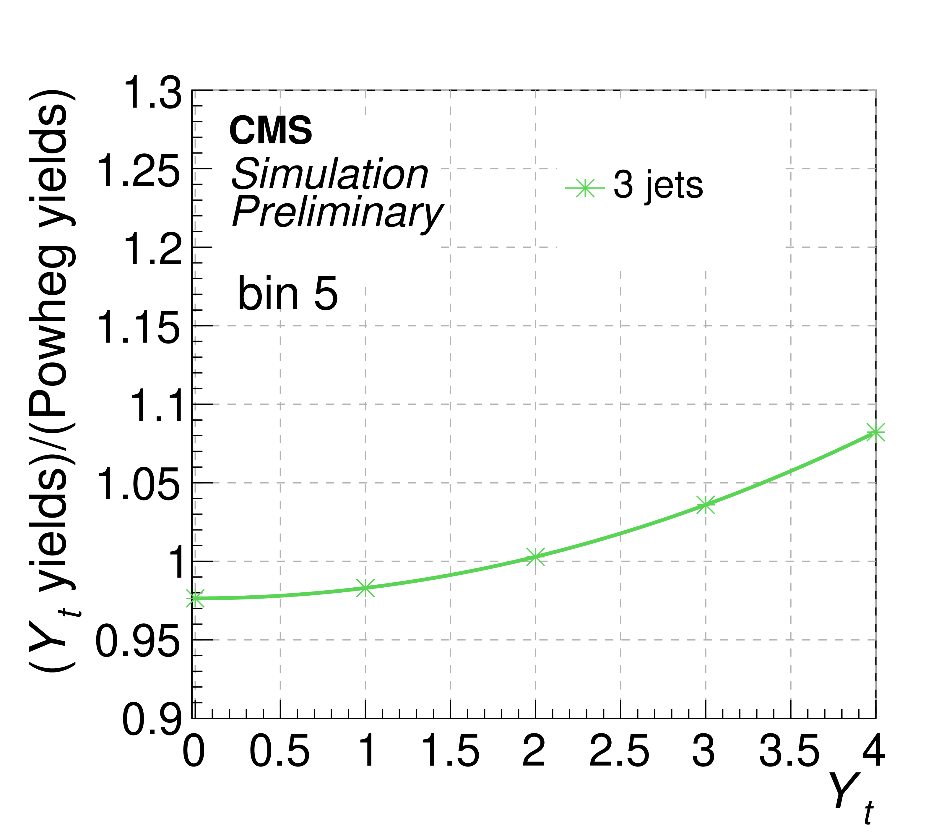
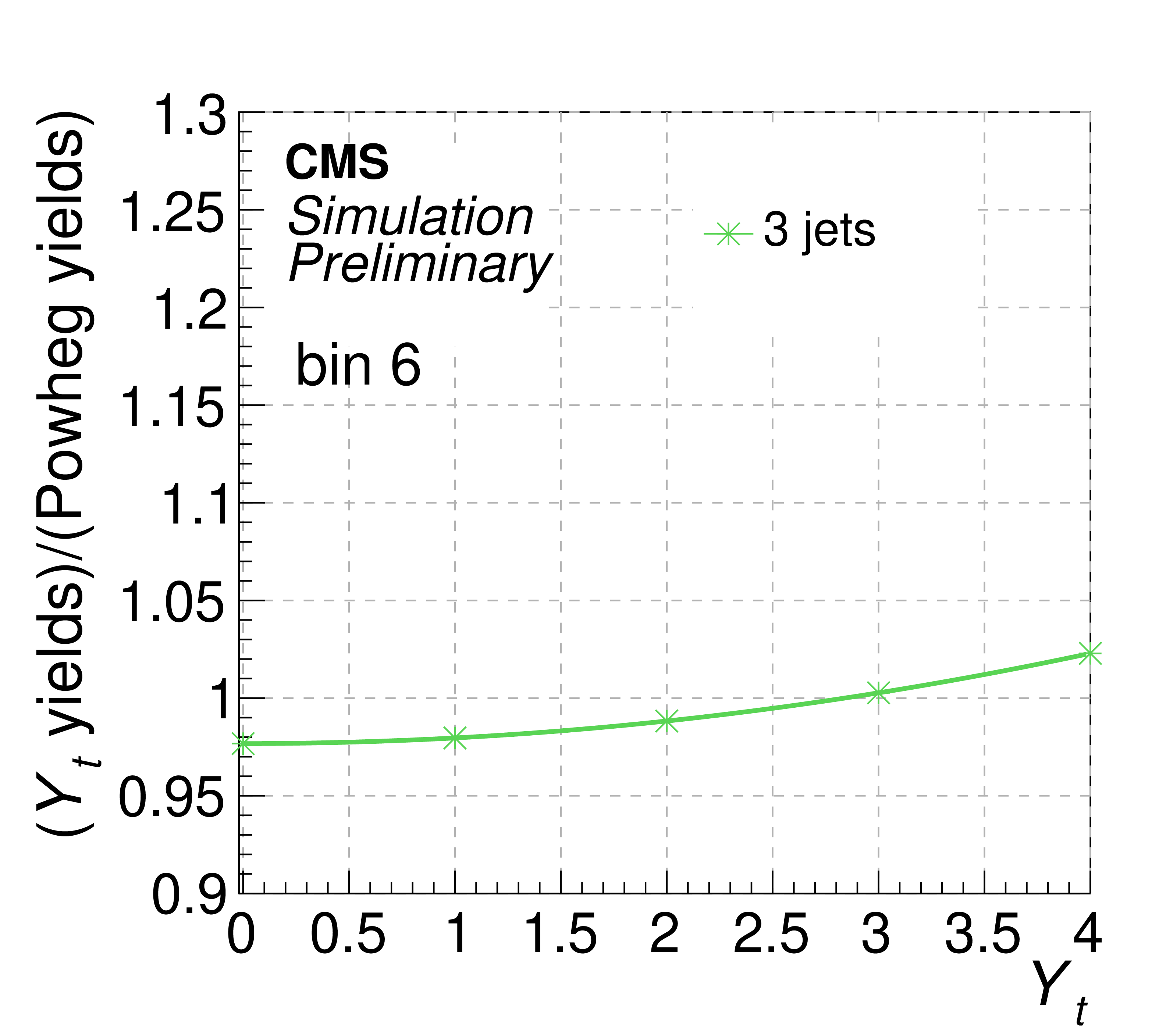
The strength of the EW correction, relative to the POWHEG expected signal, ${R^{\mathrm {bin}}(Y_t)}$, as a function of ${Y_{\text {t}}}$ in the three-jet category. Each plot corresponds to one of the eight ${M_{{{\mathrm {t}\overline {\mathrm {t}}}}}}$ bins for $| {\Delta y_{{{\mathrm {t}\overline {\mathrm {t}}}}}} | < $ 0.6 (see Fig. 10). A quadratic fit is performed in each bin. |
png pdf |
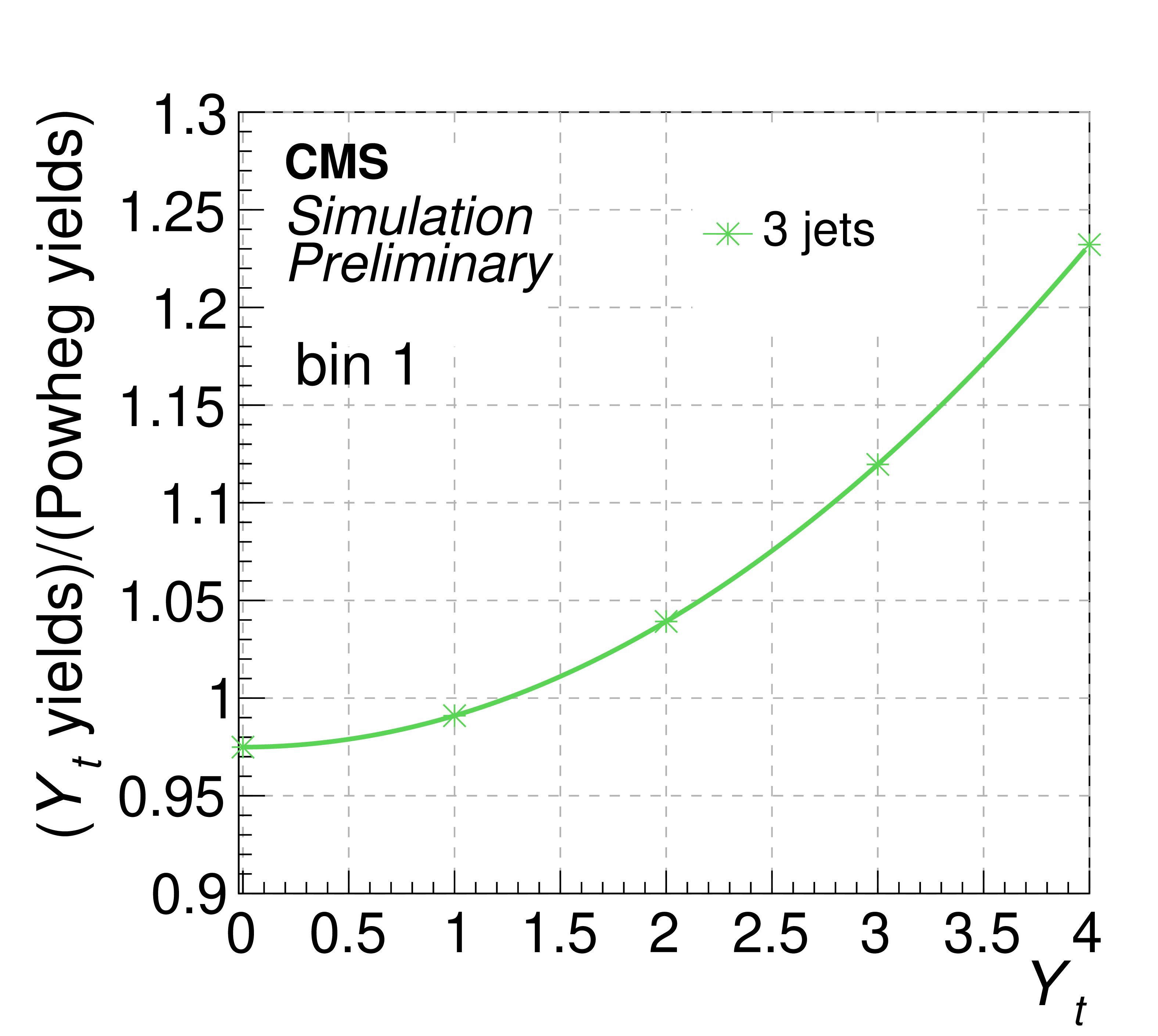
Figure 8-a:
The strength of the EW correction, relative to the POWHEG expected signal, ${R^{\mathrm {bin}}(Y_t)}$, as a function of ${Y_{\text {t}}}$ in the three-jet category. The plot corresponds to bin 1 of the eight ${M_{{{\mathrm {t}\overline {\mathrm {t}}}}}}$ bins for $| {\Delta y_{{{\mathrm {t}\overline {\mathrm {t}}}}}} | < $ 0.6 (see Fig. 10). A quadratic fit is performed. |
png pdf |
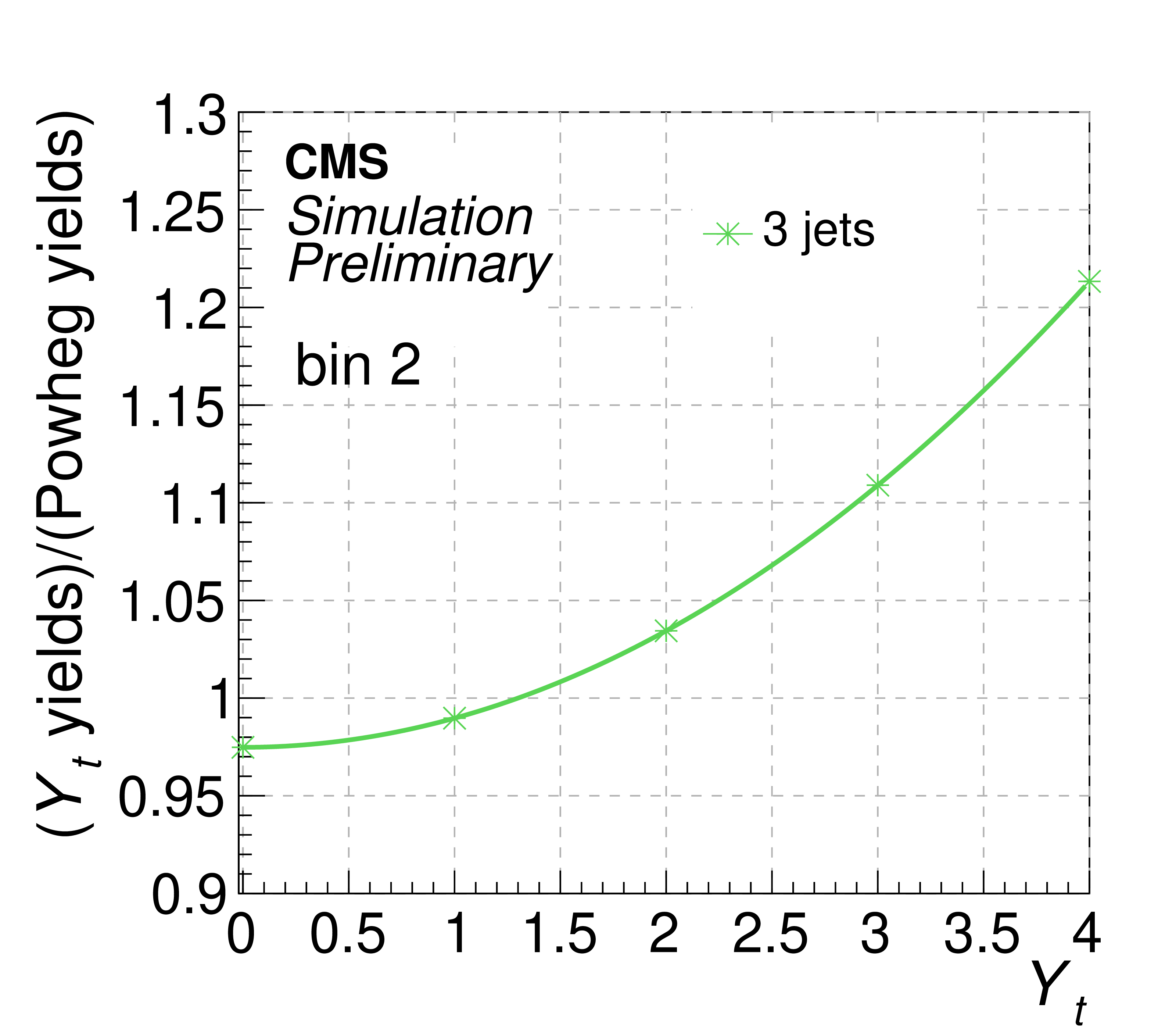
Figure 8-b:
The strength of the EW correction, relative to the POWHEG expected signal, ${R^{\mathrm {bin}}(Y_t)}$, as a function of ${Y_{\text {t}}}$ in the three-jet category. The plot corresponds to bin 2 of the eight ${M_{{{\mathrm {t}\overline {\mathrm {t}}}}}}$ bins for $| {\Delta y_{{{\mathrm {t}\overline {\mathrm {t}}}}}} | < $ 0.6 (see Fig. 10). A quadratic fit is performed. |
png pdf |
Figure 8-c:
The strength of the EW correction, relative to the POWHEG expected signal, ${R^{\mathrm {bin}}(Y_t)}$, as a function of ${Y_{\text {t}}}$ in the three-jet category. The plot corresponds to bin 3 of the eight ${M_{{{\mathrm {t}\overline {\mathrm {t}}}}}}$ bins for $| {\Delta y_{{{\mathrm {t}\overline {\mathrm {t}}}}}} | < $ 0.6 (see Fig. 10). A quadratic fit is performed. |
png pdf |
Figure 8-d:
The strength of the EW correction, relative to the POWHEG expected signal, ${R^{\mathrm {bin}}(Y_t)}$, as a function of ${Y_{\text {t}}}$ in the three-jet category. The plot corresponds to bin 4 of the eight ${M_{{{\mathrm {t}\overline {\mathrm {t}}}}}}$ bins for $| {\Delta y_{{{\mathrm {t}\overline {\mathrm {t}}}}}} | < $ 0.6 (see Fig. 10). A quadratic fit is performed. |
png pdf |
Figure 8-e:
The strength of the EW correction, relative to the POWHEG expected signal, ${R^{\mathrm {bin}}(Y_t)}$, as a function of ${Y_{\text {t}}}$ in the three-jet category. The plot corresponds to bin 5 of the eight ${M_{{{\mathrm {t}\overline {\mathrm {t}}}}}}$ bins for $| {\Delta y_{{{\mathrm {t}\overline {\mathrm {t}}}}}} | < $ 0.6 (see Fig. 10). A quadratic fit is performed. |
png pdf |
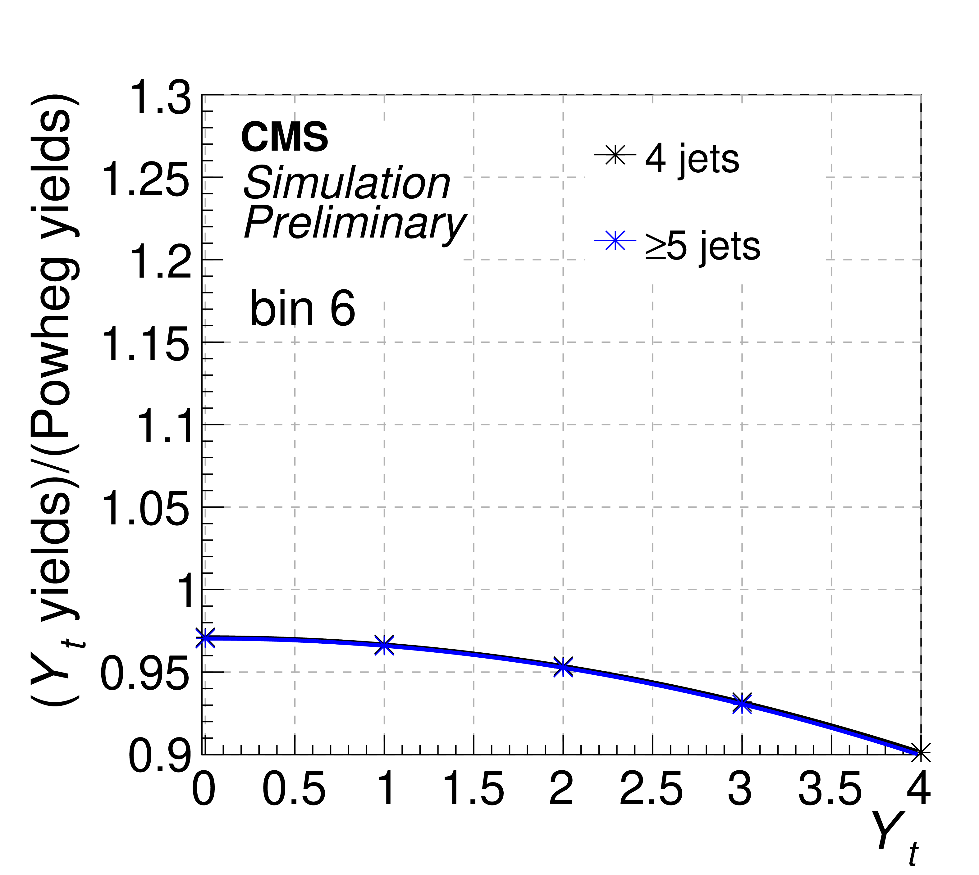
Figure 8-f:
The strength of the EW correction, relative to the POWHEG expected signal, ${R^{\mathrm {bin}}(Y_t)}$, as a function of ${Y_{\text {t}}}$ in the three-jet category. The plot corresponds to bin 6 of the eight ${M_{{{\mathrm {t}\overline {\mathrm {t}}}}}}$ bins for $| {\Delta y_{{{\mathrm {t}\overline {\mathrm {t}}}}}} | < $ 0.6 (see Fig. 10). A quadratic fit is performed. |
png pdf |
Figure 8-g:
The strength of the EW correction, relative to the POWHEG expected signal, ${R^{\mathrm {bin}}(Y_t)}$, as a function of ${Y_{\text {t}}}$ in the three-jet category. The plot corresponds to bin 7 of the eight ${M_{{{\mathrm {t}\overline {\mathrm {t}}}}}}$ bins for $| {\Delta y_{{{\mathrm {t}\overline {\mathrm {t}}}}}} | < $ 0.6 (see Fig. 10). A quadratic fit is performed. |
png pdf |
Figure 8-h:
The strength of the EW correction, relative to the POWHEG expected signal, ${R^{\mathrm {bin}}(Y_t)}$, as a function of ${Y_{\text {t}}}$ in the three-jet category. The plot corresponds to bin 8 of the eight ${M_{{{\mathrm {t}\overline {\mathrm {t}}}}}}$ bins for $| {\Delta y_{{{\mathrm {t}\overline {\mathrm {t}}}}}} | < $ 0.6 (see Fig. 10). A quadratic fit is performed. |
png pdf |
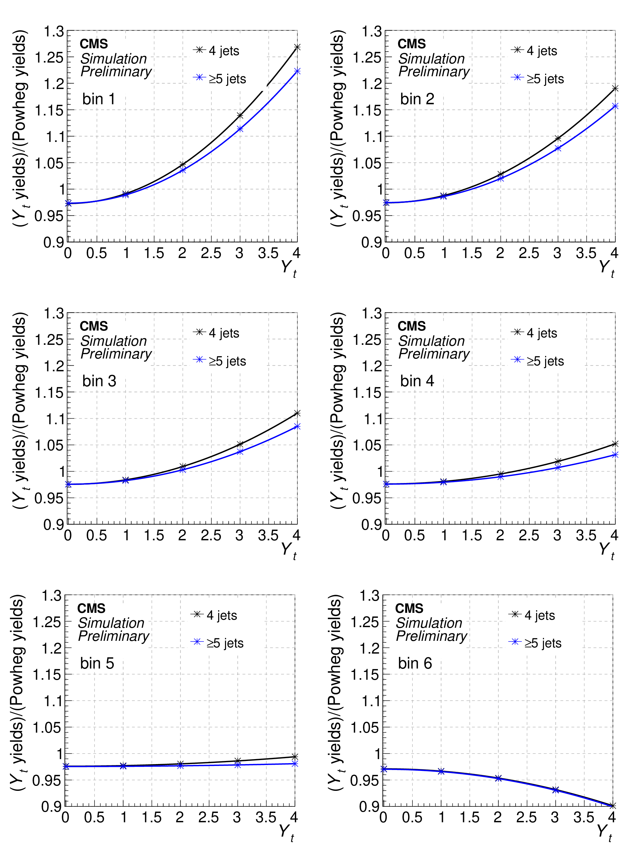
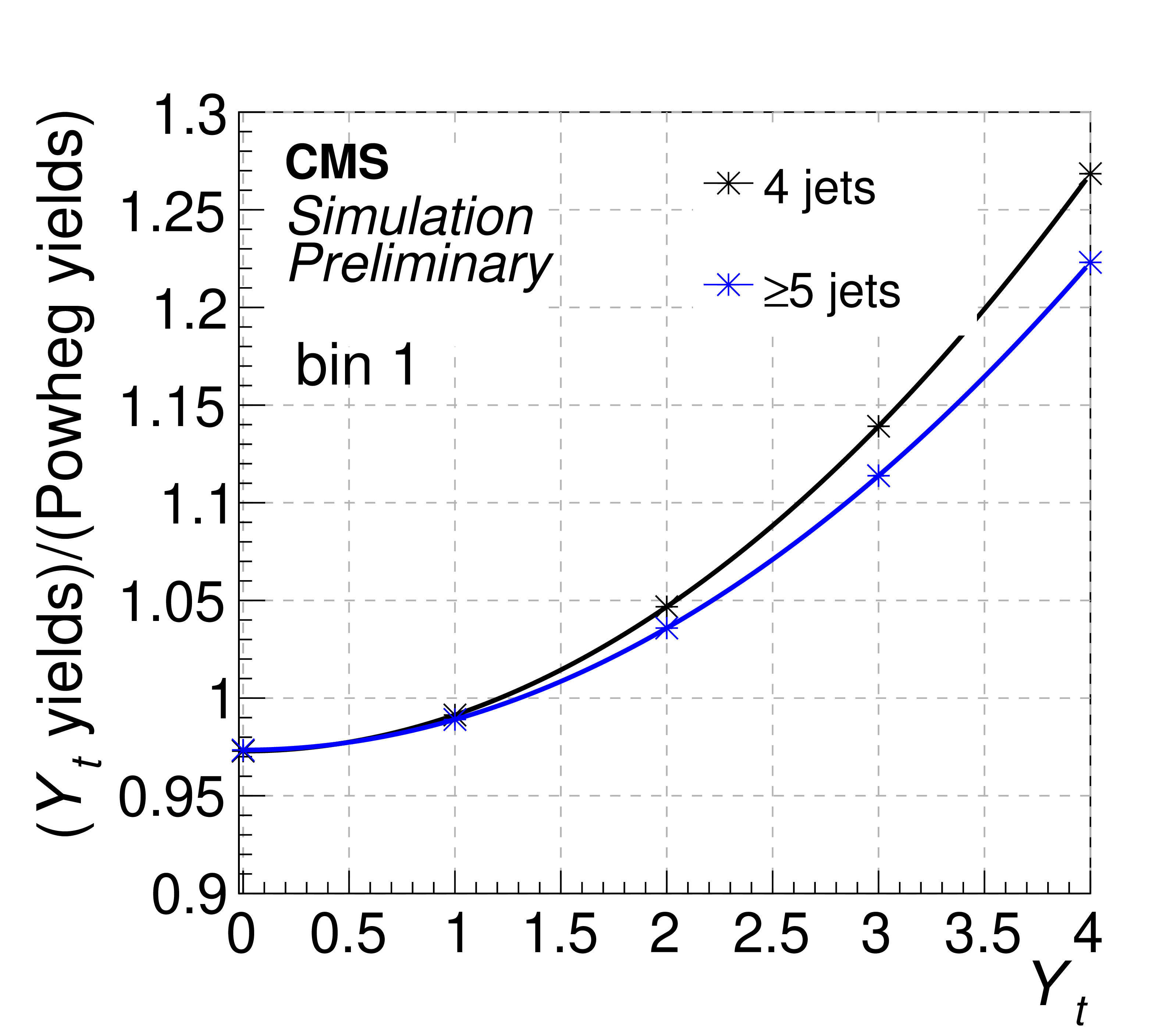
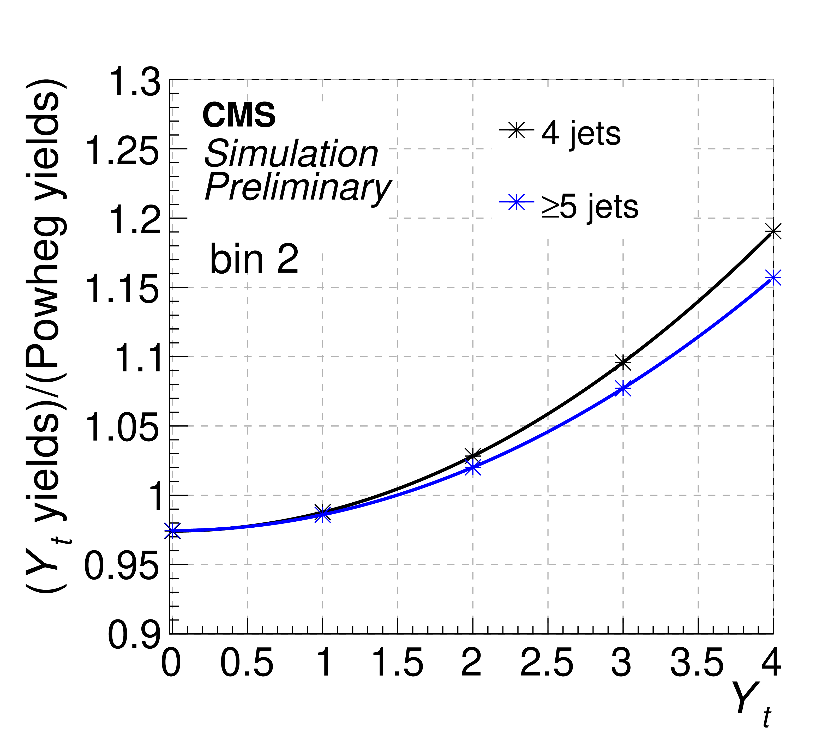
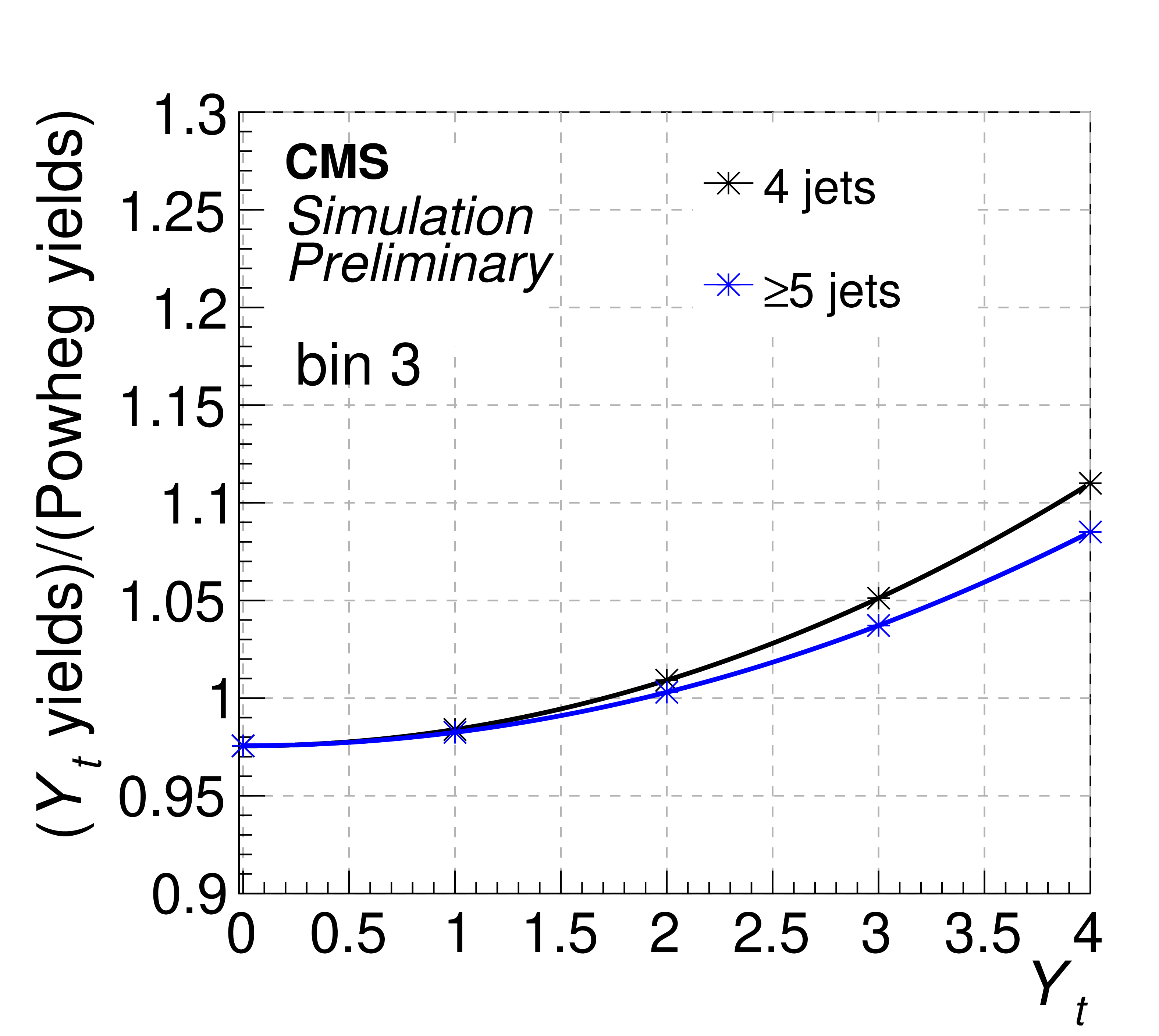
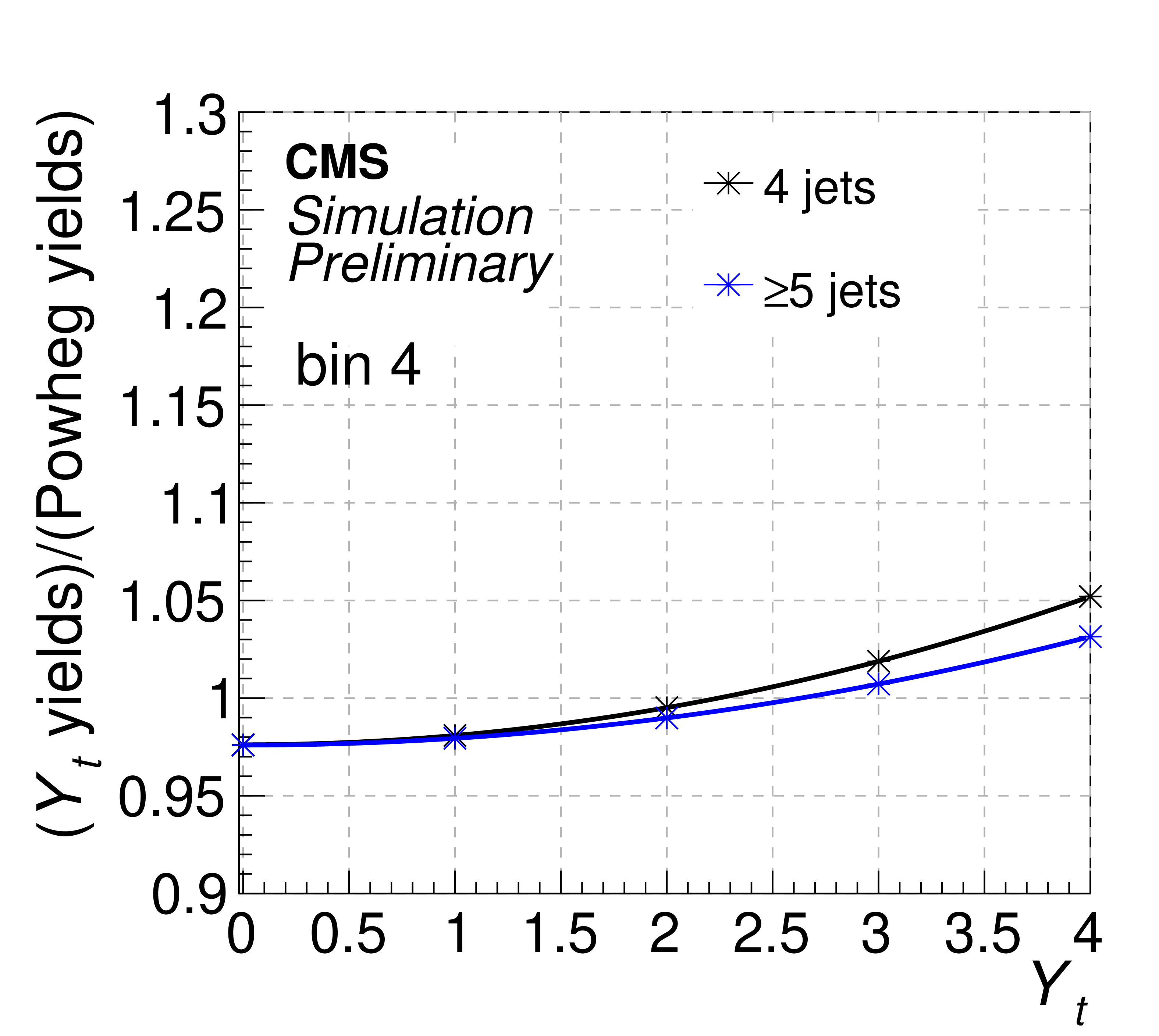
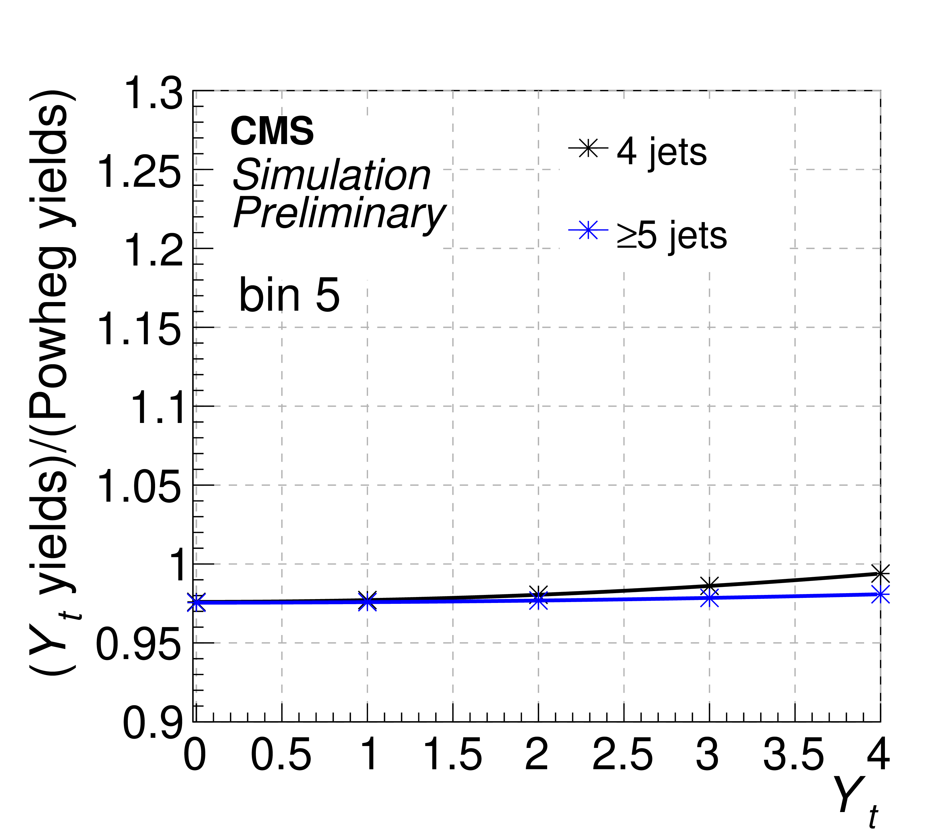
Figure 9:
The strength of the EW correction, relative to the POWHEG expected signal, ${R^{\mathrm {bin}}(Y_t)}$, as a function of ${Y_{\text {t}}}$ in the categories with four and five or more jets. Each plot corresponds to one of the six ${M_{{{\mathrm {t}\overline {\mathrm {t}}}}}}$ bins for $| {\Delta y_{{{\mathrm {t}\overline {\mathrm {t}}}}}} | < $ 0.6 (see Fig. 10). A quadratic fit is performed in each bin. |
png pdf |
Figure 9-a:
The strength of the EW correction, relative to the POWHEG expected signal, ${R^{\mathrm {bin}}(Y_t)}$, as a function of ${Y_{\text {t}}}$ in the categories with four and five or more jets. Each plot corresponds to bin 1 of the six ${M_{{{\mathrm {t}\overline {\mathrm {t}}}}}}$ bins for $| {\Delta y_{{{\mathrm {t}\overline {\mathrm {t}}}}}} | < $ 0.6 (see Fig. 10). A quadratic fit is performed. |
png pdf |
Figure 9-b:
The strength of the EW correction, relative to the POWHEG expected signal, ${R^{\mathrm {bin}}(Y_t)}$, as a function of ${Y_{\text {t}}}$ in the categories with four and five or more jets. Each plot corresponds to bin 2 of the six ${M_{{{\mathrm {t}\overline {\mathrm {t}}}}}}$ bins for $| {\Delta y_{{{\mathrm {t}\overline {\mathrm {t}}}}}} | < $ 0.6 (see Fig. 10). A quadratic fit is performed. |
png pdf |
Figure 9-c:
The strength of the EW correction, relative to the POWHEG expected signal, ${R^{\mathrm {bin}}(Y_t)}$, as a function of ${Y_{\text {t}}}$ in the categories with four and five or more jets. Each plot corresponds to bin 3 of the six ${M_{{{\mathrm {t}\overline {\mathrm {t}}}}}}$ bins for $| {\Delta y_{{{\mathrm {t}\overline {\mathrm {t}}}}}} | < $ 0.6 (see Fig. 10). A quadratic fit is performed. |
png pdf |
Figure 9-d:
The strength of the EW correction, relative to the POWHEG expected signal, ${R^{\mathrm {bin}}(Y_t)}$, as a function of ${Y_{\text {t}}}$ in the categories with four and five or more jets. Each plot corresponds to bin 4 of the six ${M_{{{\mathrm {t}\overline {\mathrm {t}}}}}}$ bins for $| {\Delta y_{{{\mathrm {t}\overline {\mathrm {t}}}}}} | < $ 0.6 (see Fig. 10). A quadratic fit is performed. |
png pdf |
Figure 9-e:
The strength of the EW correction, relative to the POWHEG expected signal, ${R^{\mathrm {bin}}(Y_t)}$, as a function of ${Y_{\text {t}}}$ in the categories with four and five or more jets. Each plot corresponds to bin 5 of the six ${M_{{{\mathrm {t}\overline {\mathrm {t}}}}}}$ bins for $| {\Delta y_{{{\mathrm {t}\overline {\mathrm {t}}}}}} | < $ 0.6 (see Fig. 10). A quadratic fit is performed. |
png pdf |
Figure 9-f:
The strength of the EW correction, relative to the POWHEG expected signal, ${R^{\mathrm {bin}}(Y_t)}$, as a function of ${Y_{\text {t}}}$ in the categories with four and five or more jets. Each plot corresponds to bin 6 of the six ${M_{{{\mathrm {t}\overline {\mathrm {t}}}}}}$ bins for $| {\Delta y_{{{\mathrm {t}\overline {\mathrm {t}}}}}} | < $ 0.6 (see Fig. 10). A quadratic fit is performed. |
png pdf |
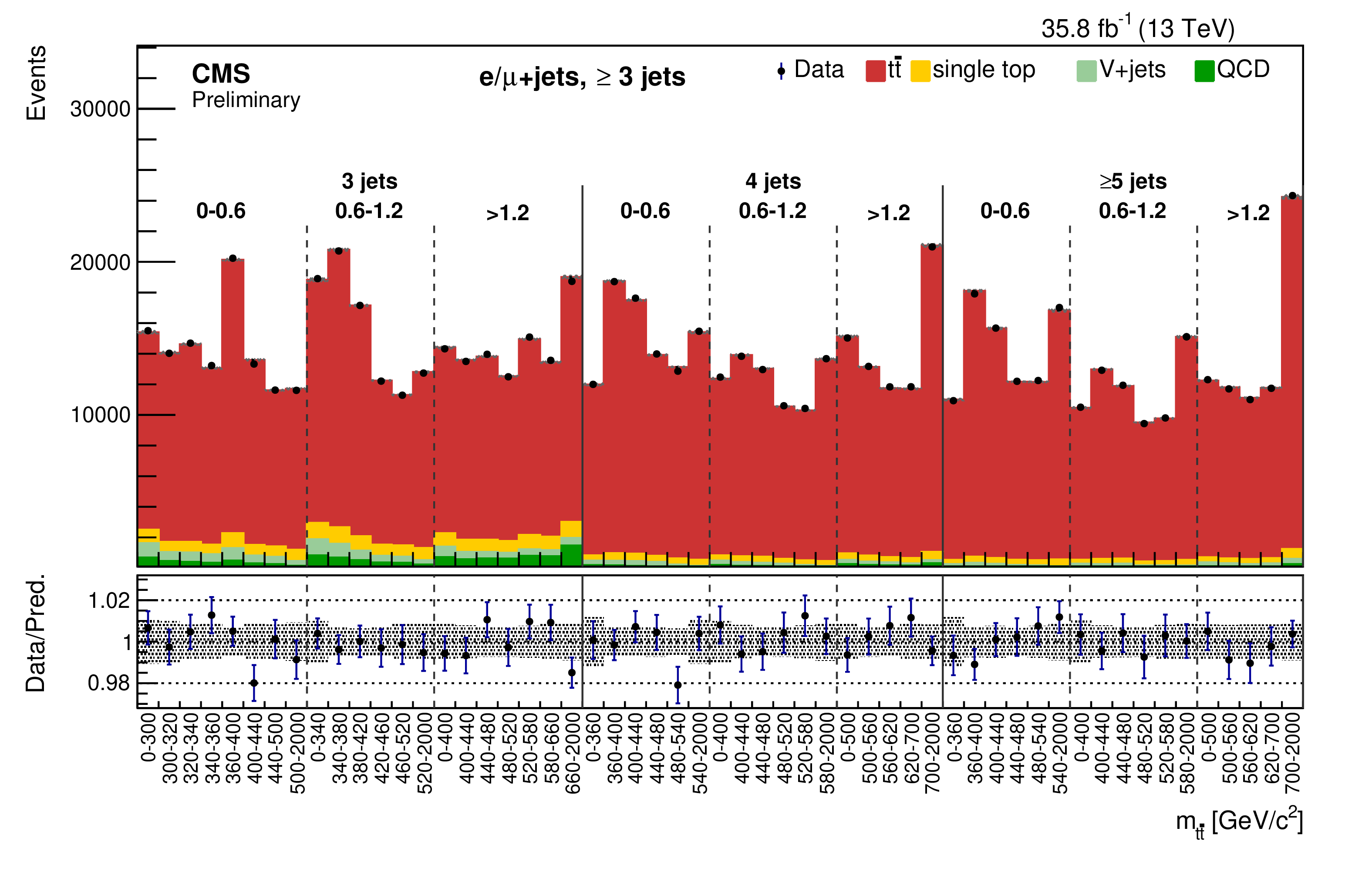
Figure 10:
The $ {M_{{{\mathrm {t}\overline {\mathrm {t}}}}}} $ distribution in $| {\Delta y_{{{\mathrm {t}\overline {\mathrm {t}}}}}} |$ bins for all channels combined, after the likelihood fit. The hatched bands show the total post-fit uncertainty. The ratios of data to the sum of the predicted yields are provided at the bottom of each panel. |
png pdf |
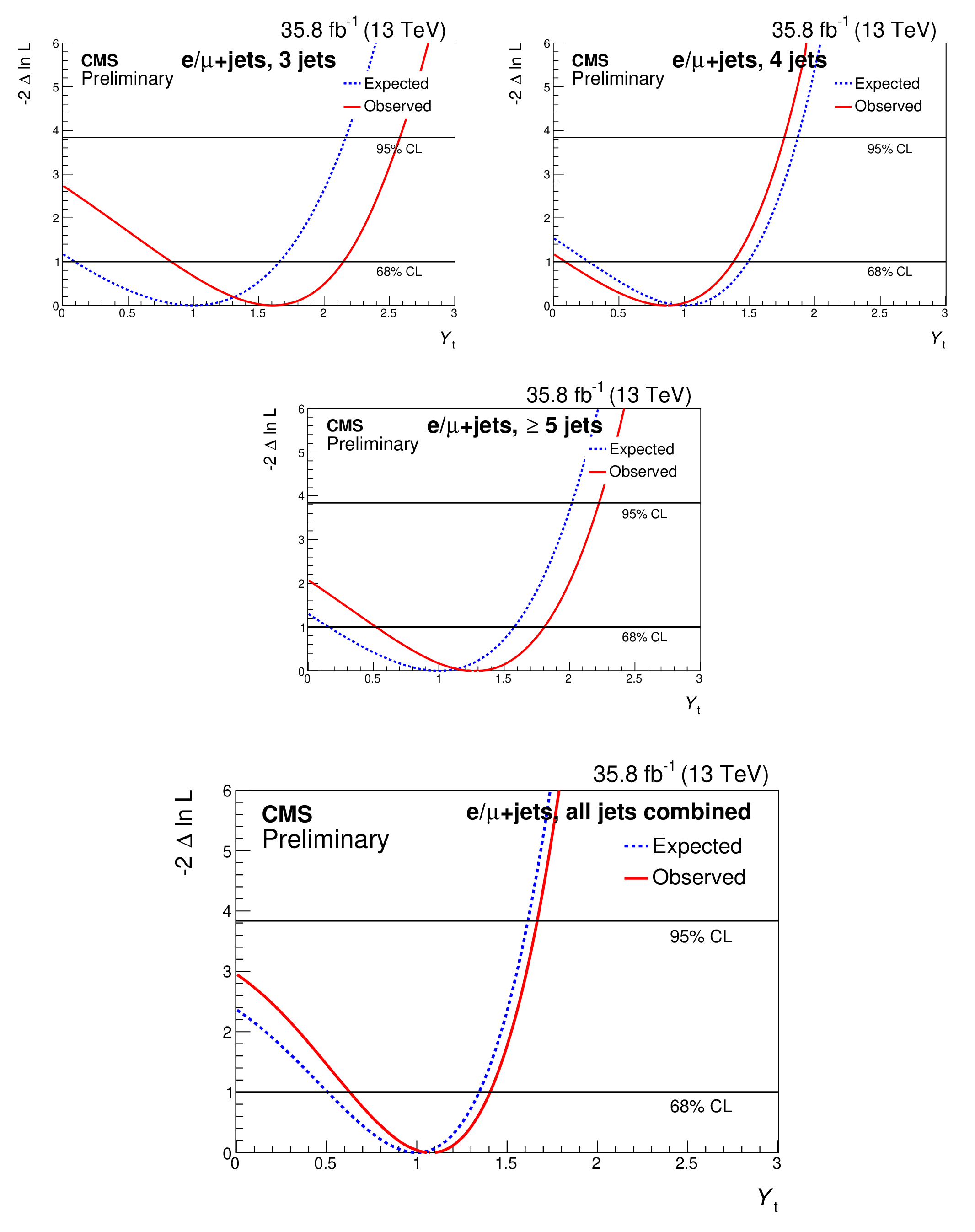
Figure 11:
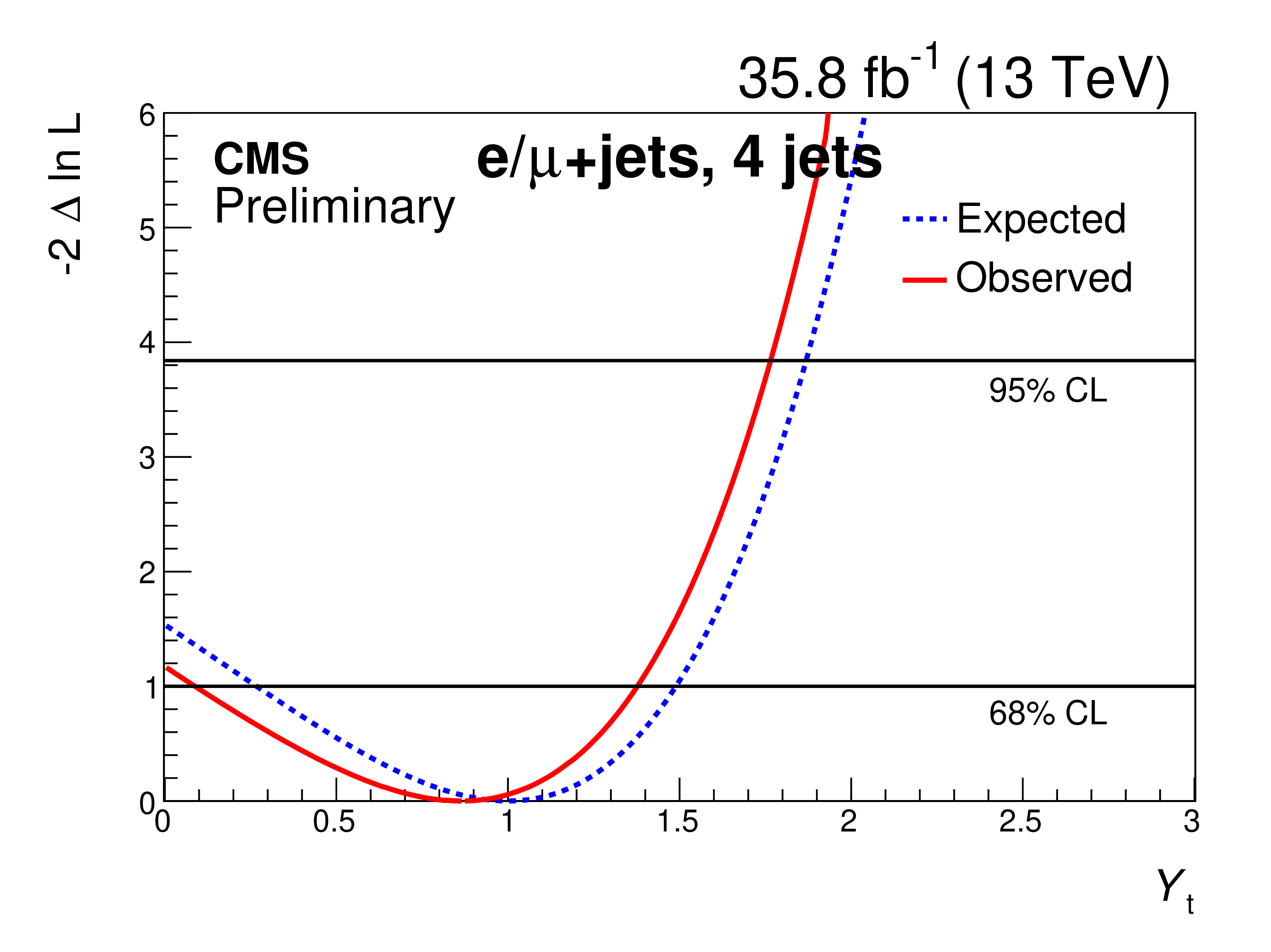
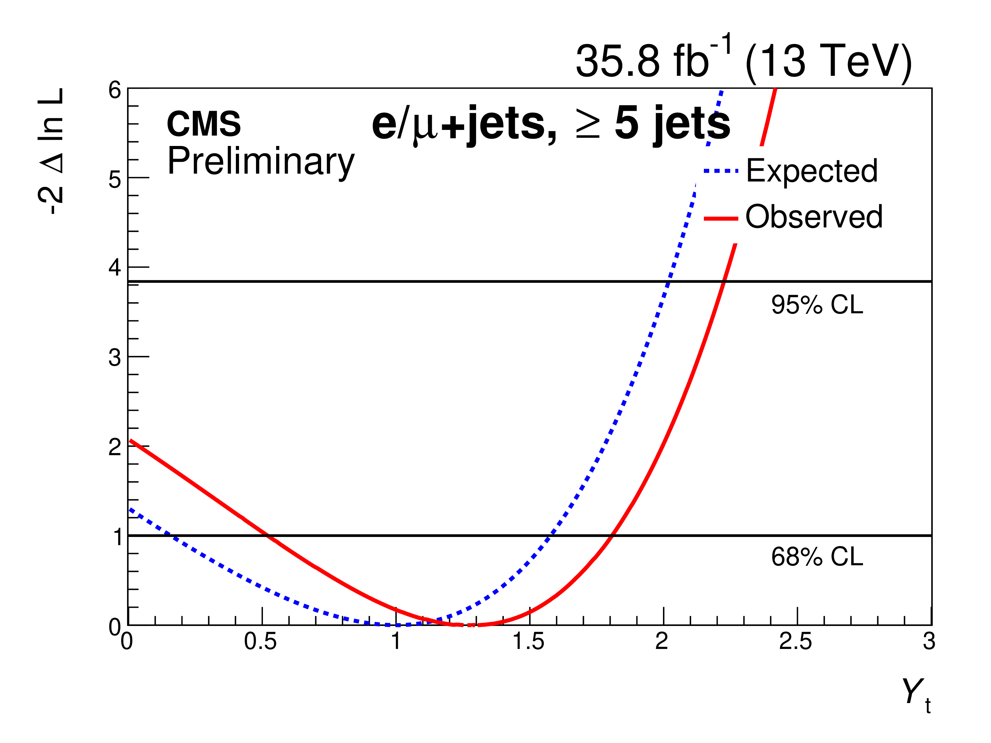
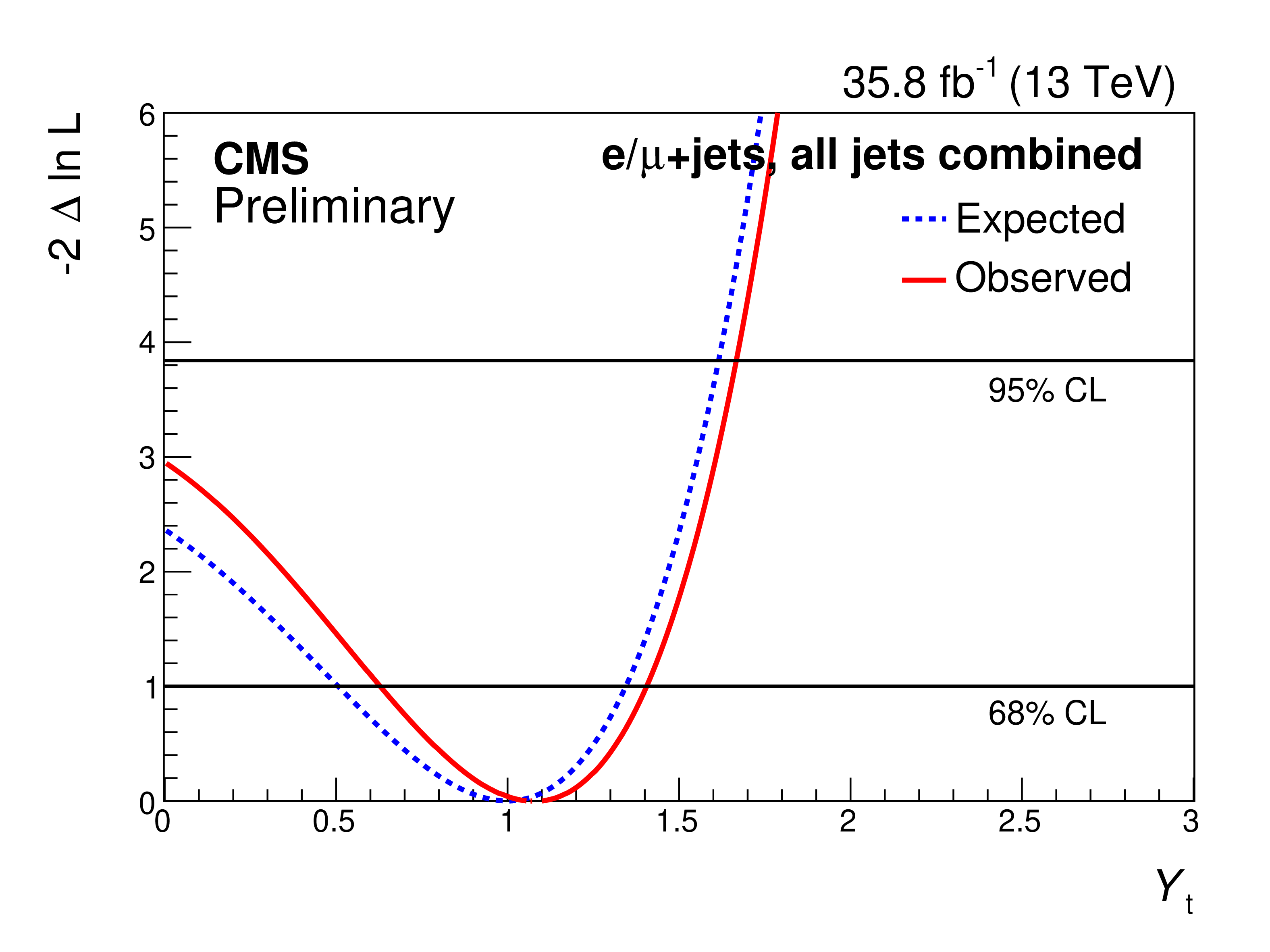
The test-statistic scan versus ${Y_{\text {t}}}$ for each channel (three jets, four jets, five or more jets), and all channels combined. The test-statistic minimum indicates the best fit of ${Y_{\text {t}}}$. The horizontal lines indicate 68% CL and 95% CL. |
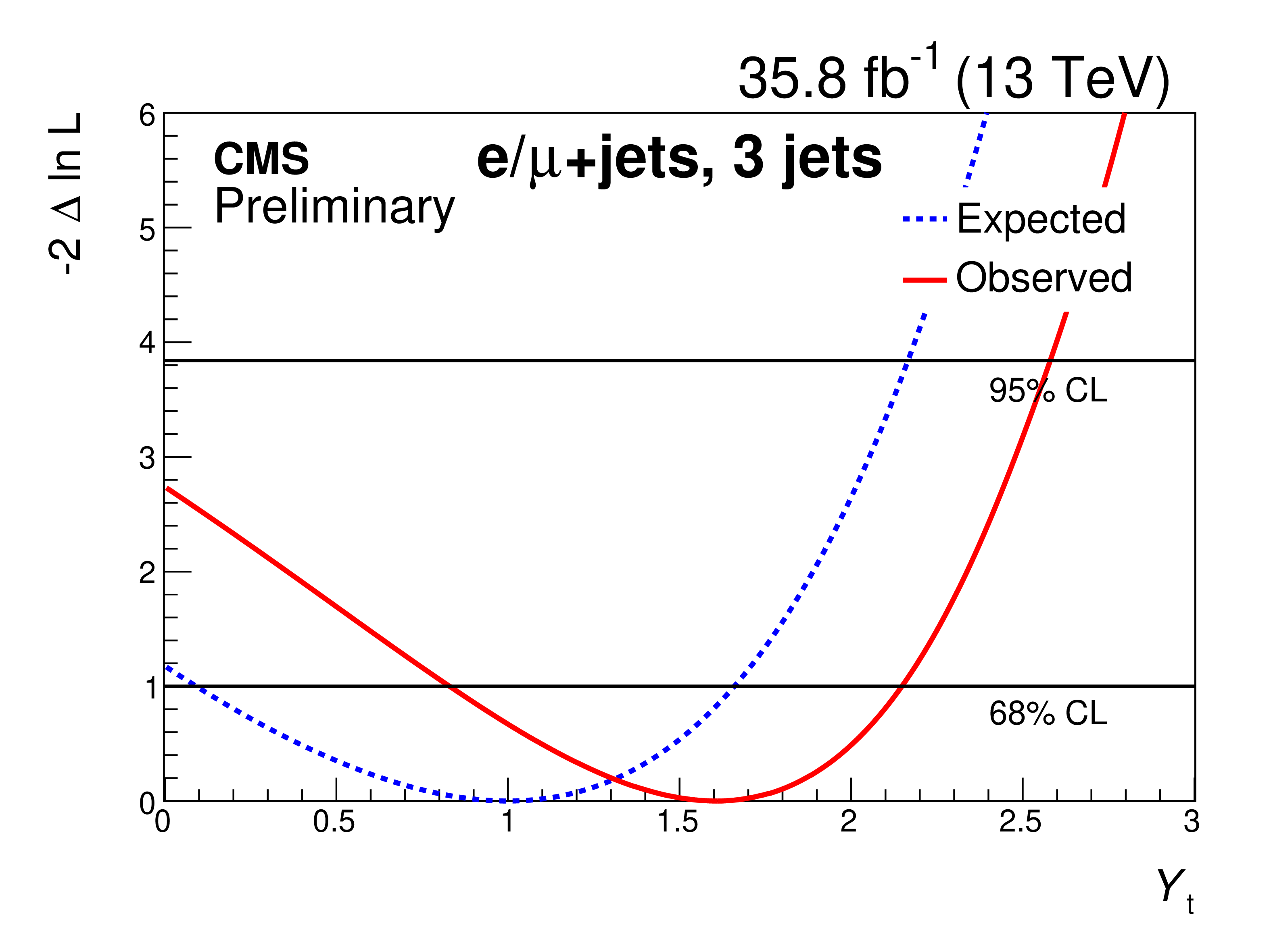
png pdf |
Figure 11-a:
The test-statistic scan versus ${Y_{\text {t}}}$ for the three-jets channel. The test-statistic minimum indicates the best fit of ${Y_{\text {t}}}$. The horizontal lines indicate 68% CL and 95% CL. |
png pdf |
Figure 11-b:
The test-statistic scan versus ${Y_{\text {t}}}$ for the four-jets channel. The test-statistic minimum indicates the best fit of ${Y_{\text {t}}}$. The horizontal lines indicate 68% CL and 95% CL. |
png pdf |
Figure 11-c:
The test-statistic scan versus ${Y_{\text {t}}}$ for the five-or-more-jets channel. The test-statistic minimum indicates the best fit of ${Y_{\text {t}}}$. The horizontal lines indicate 68% CL and 95% CL. |
png pdf |
Figure 11-d:
The test-statistic scan versus ${Y_{\text {t}}}$ for all three-jets, four-jets and five-or-more-jets channels combined. The test-statistic minimum indicates the best fit of ${Y_{\text {t}}}$. The horizontal lines indicate 68% CL and 95% CL. |
| Tables | |
png pdf |
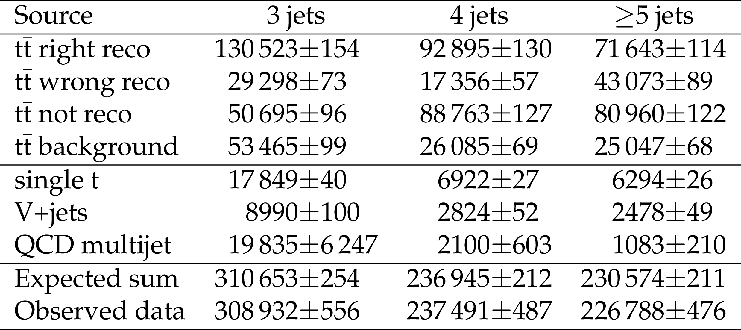
Table 1:
Expected and observed yields with statistical uncertainties after event selection. Events are categorized in the $ {{\mathrm {t}\overline {\mathrm {t}}}} $ simulation as: correctly identified $ {{\mathrm {t}\overline {\mathrm {t}}}} $ systems (${{\mathrm {t}\overline {\mathrm {t}}}}$ right); events where all decay products are available, but the $ {{\mathrm {t}\overline {\mathrm {t}}}} $ reconstruction algorithm did not identify the correct $ {{\mathrm {t}\overline {\mathrm {t}}}} $ permutation (${{\mathrm {t}\overline {\mathrm {t}}}}$ wrong); non-reconstructible events where the algorithm failed to identify at least one top candidate (${{\mathrm {t}\overline {\mathrm {t}}}}$ not reco); and events arising from the dileptonic or fully hadronic $ {{\mathrm {t}\overline {\mathrm {t}}}} $ channels (${{\mathrm {t}\overline {\mathrm {t}}}}$ background). |
png pdf |
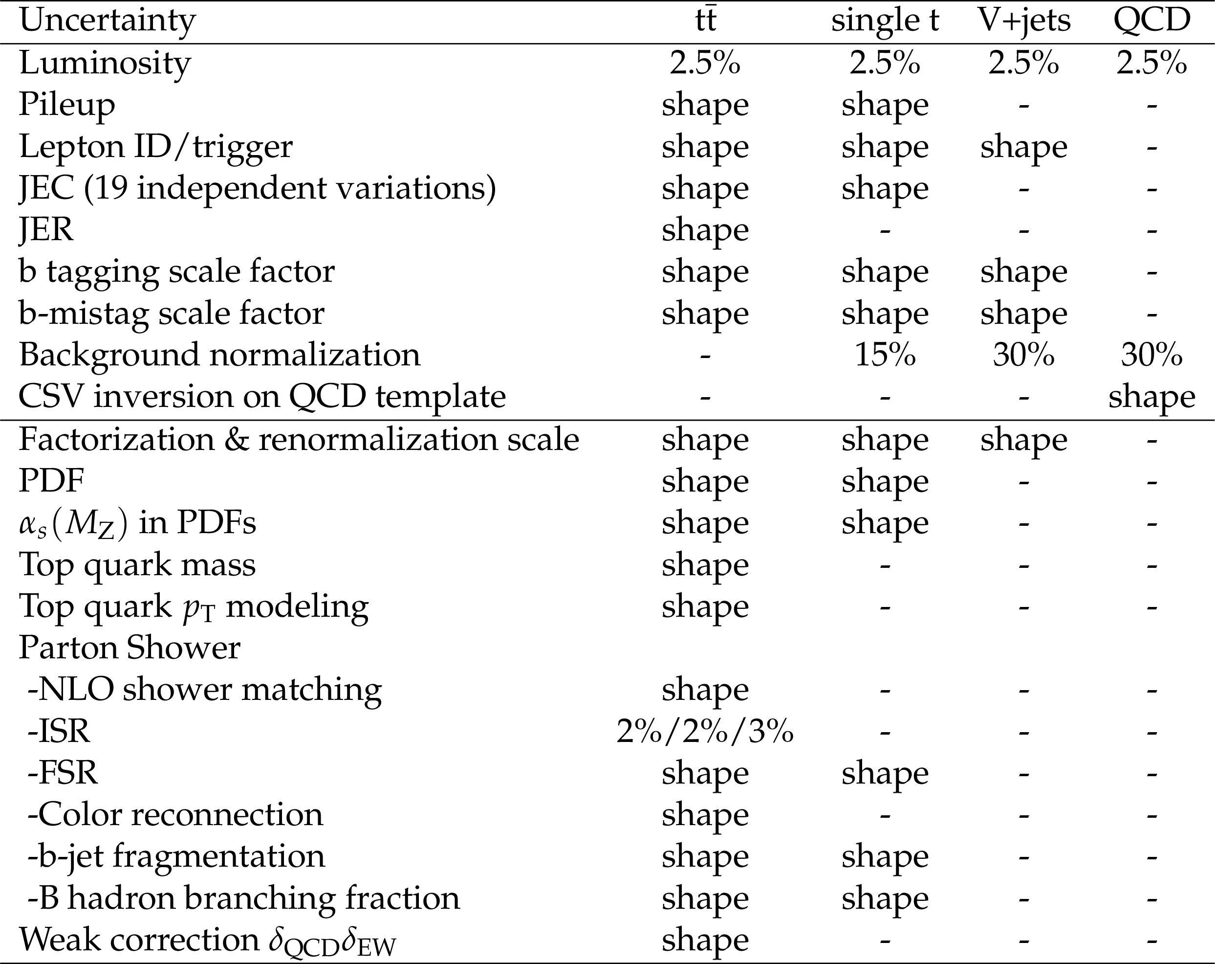
Table 2:
Summary of the sources of systematic uncertainties, their effects and magnitudes on signal and backgrounds. If the uncertainty shows a shape dependency on the ${M_{{{\mathrm {t}\overline {\mathrm {t}}}}}}$ and ${\Delta y_{{{\mathrm {t}\overline {\mathrm {t}}}}}}$ distributions, it is being considered in the likelihood and labeled as "shape'' in the table. For columns with several numbers, the numbers refer to the events with three, four, five and more jets. |
png pdf |
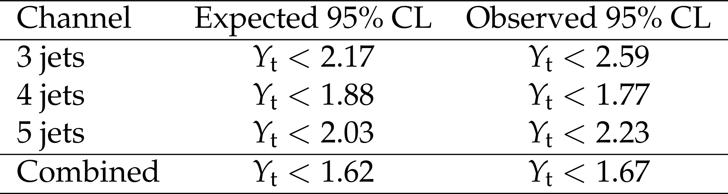
Table 3:
The expected and observed 95% CL limits on ${Y_{\text {t}}}$. |
| Summary |
| A limit on the top quark Yukawa coupling is presented, extracted by investigating top lepton+jets decays into a muon or electron and several jets in 35.8 fb$^{-1}$ of CMS data at $\sqrt{s} = $ 13 TeV. The $\mathrm{t\bar{t}}$ production rate is sensitive to the top quark Yukawa coupling through electroweak corrections that can modify the distributions of the mass of top quark-antiquark pairs, $ {M_{\mathrm{t\bar{t}}}} $, and the rapidity difference between top quarks/antiquarks, $\delta Y$. Top quark-antiquark pair events have been reconstructed with a novel algorithm applied to events with three or at least four reconstructed jets and two b tags. The inclusion of events where only three jets are reconstructed (one missing jet in the leading order lepton+jets topology) improves the sensitivity of the analysis by including more events from the low $ {M_{\mathrm{t\bar{t}}}} $ region, which is most sensitive to the Yukawa coupling. The top quark Yukawa coupling is extracted by comparing the data with the expected $\mathrm{t\bar{t}}$ signal for different values of $ {Y_{\text{t}}} $ in a total of 57 bins in $ {M_{\mathrm{t\bar{t}}}} $, $\delta Y$, and the number of reconstructed jets. The value of the top quark Yukawa coupling is constrained to be less than 1.67 at the 95% confidence level. |
| References | ||||
| 1 | M. Czakon et al. | Top-pair production at the LHC through NNLO QCD and NLO EW | JHEP 10 (2017) 186 | 1705.04105 |
| 2 | M. L. Czakon et al. | Top quark pair production at NNLO+NNLL$ ' $ in QCD combined with electroweak corrections | in 11th International Workshop on Top Quark Physics (TOP2018) Bad Neuenahr, Germany 2018-2019 | 1901.08281 |
| 3 | J. H. Kuhn, A. Scharf, and P. Uwer | Weak Interactions in Top-Quark Pair Production at Hadron Colliders: An Update | PRD 91 (2015) 014020 | 1305.5773 |
| 4 | CMS Collaboration | Measurement of differential cross sections for top quark pair production using the lepton+jets final state in proton-proton collisions at 13 TeV | PRD95 (2017) 092001 | CMS-TOP-16-008 1610.04191 |
| 5 | M. Aliev et al. | HATHOR: HAdronic Top and Heavy quarks crOss section calculatoR | CPC 182 (2011) 1034 | 1007.1327 |
| 6 | CMS Collaboration | Measurement of differential cross sections for the production of top quark pairs and of additional jets in lepton+jets events from pp collisions at $ \sqrt{s} = $ 13 TeV | PRD97 (2018) 112003 | CMS-TOP-17-002 1803.08856 |
| 7 | W. Beenakker et al. | Electroweak one loop contributions to top pair production in hadron colliders | NPB411 (1994) 343 | |
| 8 | P. Nason | A new method for combining NLO QCD with shower Monte Carlo algorithms | JHEP 11 (2004) 040 | hep-ph/0409146 |
| 9 | S. Frixione, P. Nason, and C. Oleari | Matching NLO QCD computations with Parton Shower simulations: the POWHEG method | JHEP 11 (2007) 070 | 0709.2092 |
| 10 | S. Alioli, P. Nason, C. Oleari, and E. Re | A general framework for implementing NLO calculations in shower Monte Carlo programs: the POWHEG BOX | JHEP 06 (2010) 043 | 1002.2581 |
| 11 | J. M. Campbell, R. K. Ellis, P. Nason, and E. Re | Top-pair production and decay at NLO matched with parton showers | JHEP 04 (2015) 114 | 1412.1828 |
| 12 | T. Sjostrand, S. Mrenna, and P. Skands | PYTHIA 6.4 physics and manual | JHEP 05 (2006) 026 | hep-ph/0603175 |
| 13 | T. Sjostrand, S. Mrenna, and P. Z. Skands | A Brief Introduction to PYTHIA 8.1 | CPC 178 (2008) 852 | 0710.3820 |
| 14 | P. Skands, S. Carrazza, and J. Rojo | Tuning PYTHIA 8.1: the Monash 2013 Tune | EPJC 74 (2014) 3024 | 1404.5630 |
| 15 | NNPDF Collaboration | Parton distributions for the LHC Run II | JHEP 04 (2015) 040 | 1410.8849 |
| 16 | M. Czakon and A. Mitov | Top++: A Program for the Calculation of the Top-Pair Cross-Section at Hadron Colliders | CPC 185 (2014) 2930 | 1112.5675 |
| 17 | J. Alwall et al. | The automated computation of tree-level and next-to-leading order differential cross sections, and their matching to parton shower simulations | JHEP 07 (2014) 079 | 1405.0301 |
| 18 | Y. Li and F. Petriello | Combining QCD and electroweak corrections to dilepton production in FEWZ | PRD 86 (2012) 094034 | 1208.5967 |
| 19 | P. Kant et al. | HATHOR for single top-quark production: Updated predictions and uncertainty estimates for single top-quark production in hadronic collisions | CPC 191 (2015) 74 | 1406.4403 |
| 20 | N. Kidonakis | NNLL threshold resummation for top-pair and single-top production | Phys. Part. Nucl. 45 (2014) 714 | 1210.7813 |
| 21 | J. Allison et al. | Geant4 developments and applications | IEEE Trans. Nucl. Sci. 53 (2006) 270 | |
| 22 | M. Cacciari, G. P. Salam, and G. Soyez | The anti-$ k_t $ jet clustering algorithm | JHEP 2008 (2008) 063 | |
| 23 | M. Cacciari, G. P. Salam, and G. Soyez | Fastjet user manual | The European Physical Journal C 72 (2012), no. 3 | |
| 24 | T. C. collaboration | Determination of jet energy calibration and transverse momentum resolution in CMS | JINST 6 (2011) P11002 | |
| 25 | CMS Collaboration | Jet energy scale and resolution in the CMS experiment in pp collisions at 8 TeV | JINST 12 (2017) P02014 | CMS-JME-13-004 1607.03663 |
| 26 | CMS Collaboration | Identification of b quark jets at the CMS Experiment in the LHC Run 2 | ||
| 27 | CMS Collaboration Collaboration | Identification of b quark jets at the CMS Experiment in the LHC Run 2 | CMS-PAS-BTV-15-001, CERN | |
| 28 | CMS Collaboration | Measurement of inclusive W and Z boson production cross sections in pp collisions at $ \sqrt{s} = $ 8 TeV | PRL 112 (2014) 191802 | CMS-SMP-12-011 1402.0923 |
| 29 | B. A. Betchart, R. Demina, and A. Harel | Analytic solutions for neutrino momenta in decay of top quarks | NIMA 736 (2014) 169 | 1305.1878 |
| 30 | R. Demina, A. Harel, and D. Orbaker | Reconstructing events with one lost jet | Nuclear Instruments and Methods in Physics Research Section A: Accelerators, Spectrometers, Detectors and Associated Equipment 788 (2015) 128 | |
| 31 | The ATLAS Collaboration, The CMS Collaboration, The LHC Higgs Combination Group Collaboration | Procedure for the LHC Higgs boson search combination in Summer 2011 | CMS-NOTE-2011-005 | |
| 32 | ATLAS and CMS developers | Higgs Analysis Combined Limit | v.5.0.4 for ROOT 6 SLC6 release | |
| 33 | CMS Collaboration | CMS Luminosity Measurement for the 2016 Data Taking Period | ||
| 34 | CMS Collaboration | Performance of electron reconstruction and selection with the CMS detector in proton-proton collisions at $ \sqrt{s}= $ 8 TeV | ``Performance of electron reconstruction and selection with the CMS detector in proton-proton collisions at $\sqrt{s}=$ 8 TeV'', JINST 10 (2015) P06005 | |
| 35 | CMS Collaboration | Performance of the CMS muon detector and muon reconstruction with proton-proton collisions at $ \sqrt{s}= $ 13 TeV | JINST 13 (2018) P06015 | CMS-MUO-16-001 1804.04528 |
| 36 | LHC Top WG | WG Summary Plots | Accessed: 2010-09-30 | |
| 37 | LHC EWK WG | WG Summary Plots | Accessed: 2010-09-30 | |
| 38 | M. Czakon, D. Heymes, and A. Mitov | fastNLO tables for NNLO top-quark pair differential distributions | 1704.08551 | |
| 39 | CMS Collaboration | Investigations of the impact of the parton shower tuning in Pythia 8 in the modelling of tt at $ \sqrt{s} = $ 8 and 13 TeV | CMS-PAS-TOP-16-021 | CMS-PAS-TOP-16-021 |
| 40 | Particle Data Group Collaboration | Review of Particle Physics | PRD98 (2018) 030001 | |
| 41 | Peter Uwer | Private Communication | during TOP Readiness Meeting on April 28, 2017 | |
| 42 | J. S. Conway | Incorporating Nuisance Parameters in Likelihoods for Multisource Spectra | in Proceedings, PHYSTAT 2011 Workshop on Statistical Issues Related to Discovery Claims in Search Experiments and Unfolding, CERN 2011 | 1103.0354 |
|
|
Compact Muon Solenoid LHC, CERN |
|

|

|

|

|

|