

Compact Muon Solenoid
LHC, CERN
| CMS-PAS-HIG-21-016 | ||
| Search for exotic Higgs boson decays H $ \rightarrow \mathcal{A}\mathcal{A} \rightarrow 4\gamma$ with events containing two merged photons in proton-proton collisions at $\sqrt{s} = $ 13 TeV | ||
| CMS Collaboration | ||
| March 2022 | ||
| Abstract: The result of a direct search for the exotic Higgs boson decay $\mathrm{H}\rightarrow\mathcal{A}\mathcal{A}$, $\mathcal{A}\rightarrow\gamma\gamma$ is presented, using events with a final state containing two photons. The hypothetical particle $\mathcal{A}$ is a low-mass, boosted scalar decaying promptly to two highly merged photons, misreconstructed as a single photon-like object. The data were collected by the CMS experiment at the CERN LHC from proton-proton collisions at $\sqrt{s} = $ 13 TeV, corresponding to an integrated luminosity of 136 fb$^{-1}$. No excess of events above the estimated background is found. Upper limits on the branching fraction $\mathcal{B}(\mathrm{H} \rightarrow \mathcal{A}\mathcal{A} \rightarrow 4\gamma)$ of 0.9--3.3$\times$10$^{-3}$ are set at the 95% confidence level for masses of $\mathcal{A}$ in the range 0.1 $ < m_{\mathcal{A}} < $ 1.2 GeV. | ||
|
Links:
CDS record (PDF) ;
CADI line (restricted) ;
These preliminary results are superseded in this paper, PRL 131 (2023) 101801. The superseded preliminary plots can be found here. |
||
| Figures | |

png pdf |
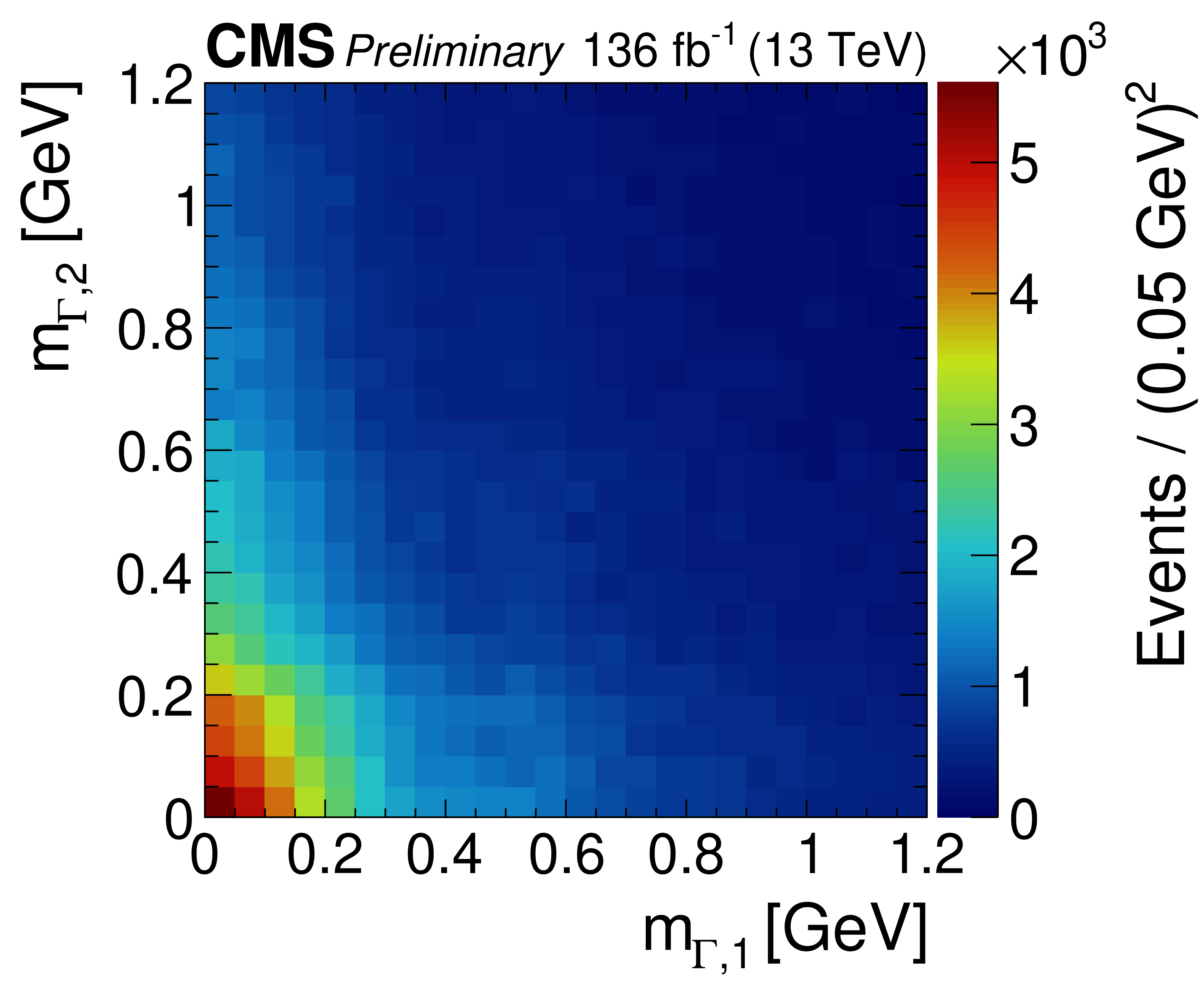
Figure 1:
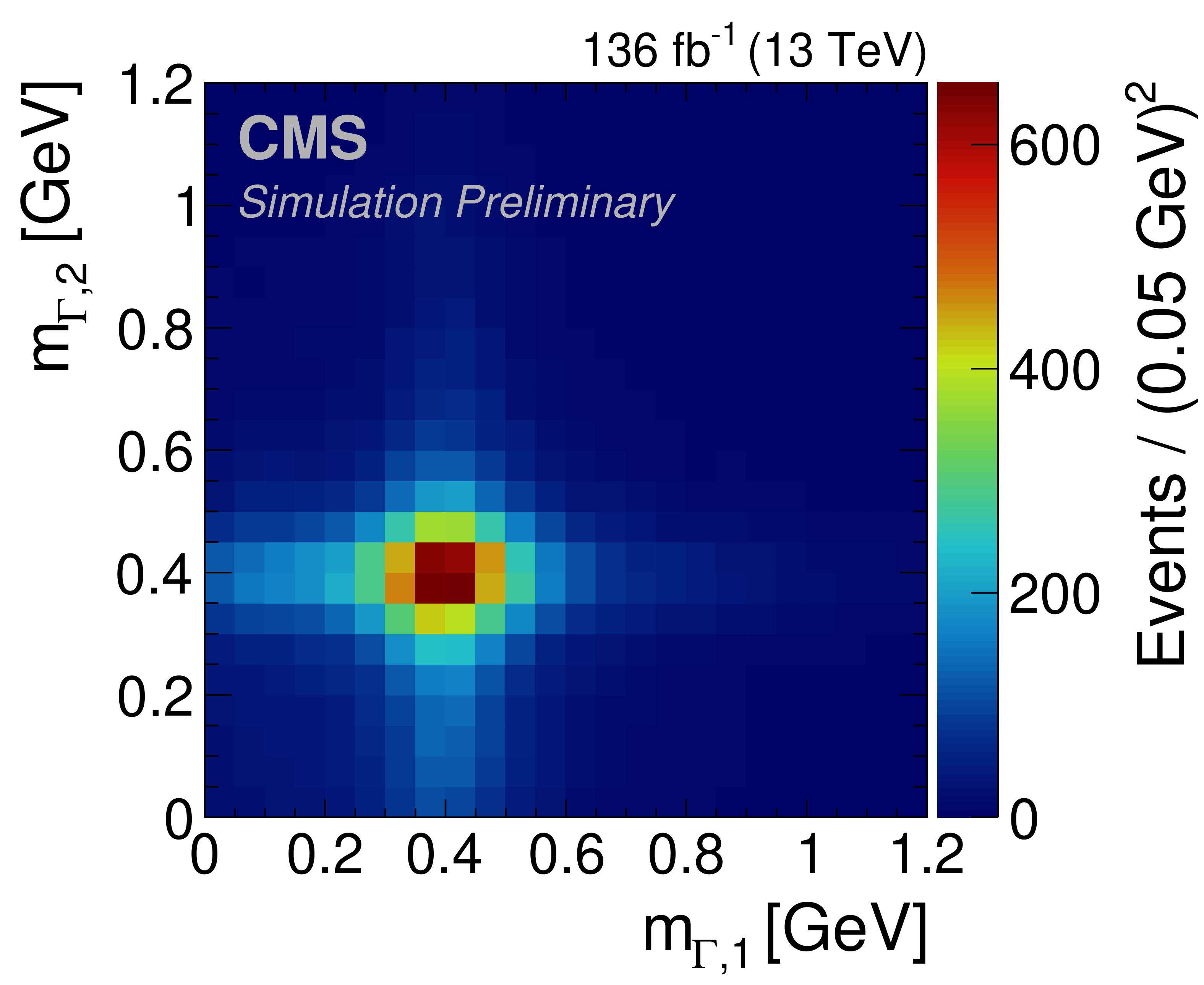
Simulated $m_{\Gamma,1}$ vs. $m_{\Gamma,2}$ 2D distributions for $\mathrm{H} \rightarrow {\mathcal {A}} {\mathcal {A}} \rightarrow 4\gamma $ events passing the selection criteria for masses $m_{{\mathcal {A}}}=$ 0.1 (left), 0.4 (center), and 1 GeV (right). The distributions are normalized to the total integrated luminosity in the studied data set, assuming a total signal cross section times branching fraction of 1 pb. The color scales to the right of each plot give the number of events per bin. |

png pdf |
Figure 1-a:
Simulated $m_{\Gamma,1}$ vs. $m_{\Gamma,2}$ 2D distributions for $\mathrm{H} \rightarrow {\mathcal {A}} {\mathcal {A}} \rightarrow 4\gamma $ events passing the selection criteria for masses $m_{{\mathcal {A}}}=$ 0.1 (left), 0.4 (center), and 1 GeV (right). The distributions are normalized to the total integrated luminosity in the studied data set, assuming a total signal cross section times branching fraction of 1 pb. The color scales to the right of each plot give the number of events per bin. |
png pdf |
Figure 1-b:
Simulated $m_{\Gamma,1}$ vs. $m_{\Gamma,2}$ 2D distributions for $\mathrm{H} \rightarrow {\mathcal {A}} {\mathcal {A}} \rightarrow 4\gamma $ events passing the selection criteria for masses $m_{{\mathcal {A}}}=$ 0.1 (left), 0.4 (center), and 1 GeV (right). The distributions are normalized to the total integrated luminosity in the studied data set, assuming a total signal cross section times branching fraction of 1 pb. The color scales to the right of each plot give the number of events per bin. |

png pdf |
Figure 1-c:
Simulated $m_{\Gamma,1}$ vs. $m_{\Gamma,2}$ 2D distributions for $\mathrm{H} \rightarrow {\mathcal {A}} {\mathcal {A}} \rightarrow 4\gamma $ events passing the selection criteria for masses $m_{{\mathcal {A}}}=$ 0.1 (left), 0.4 (center), and 1 GeV (right). The distributions are normalized to the total integrated luminosity in the studied data set, assuming a total signal cross section times branching fraction of 1 pb. The color scales to the right of each plot give the number of events per bin. |

png pdf |
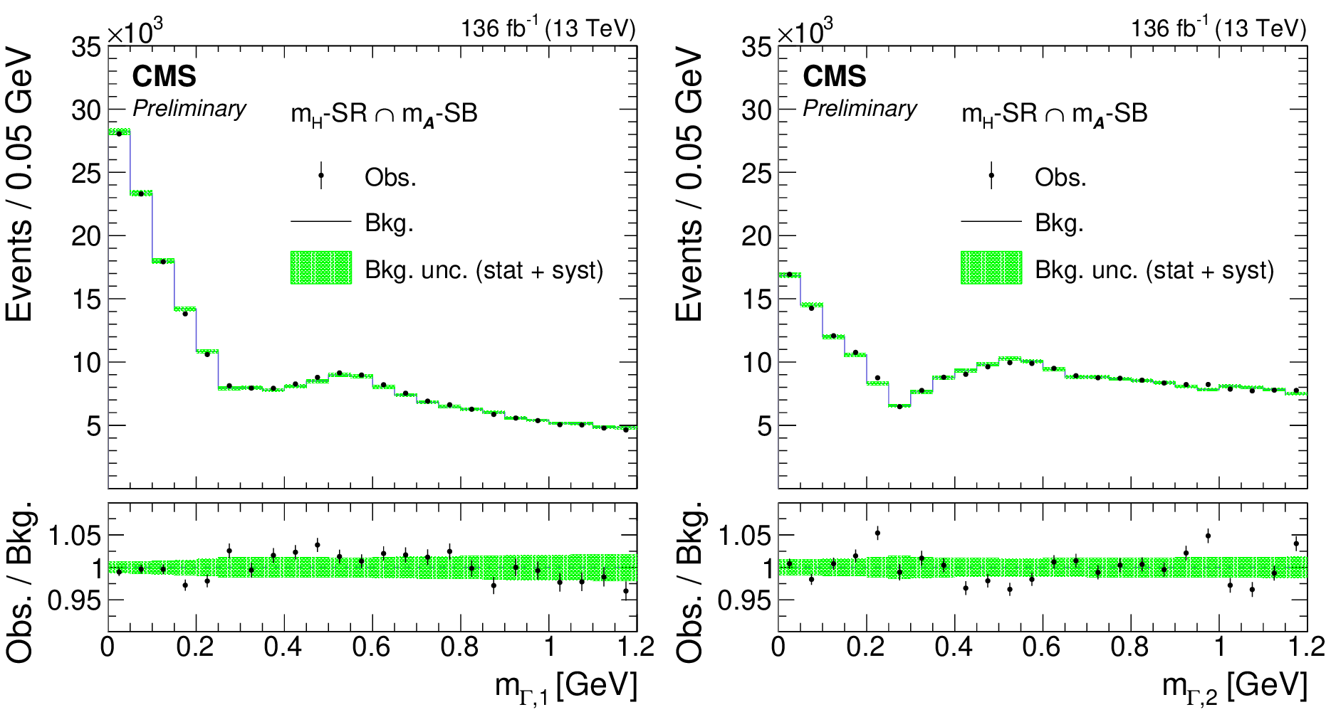
Figure 2:
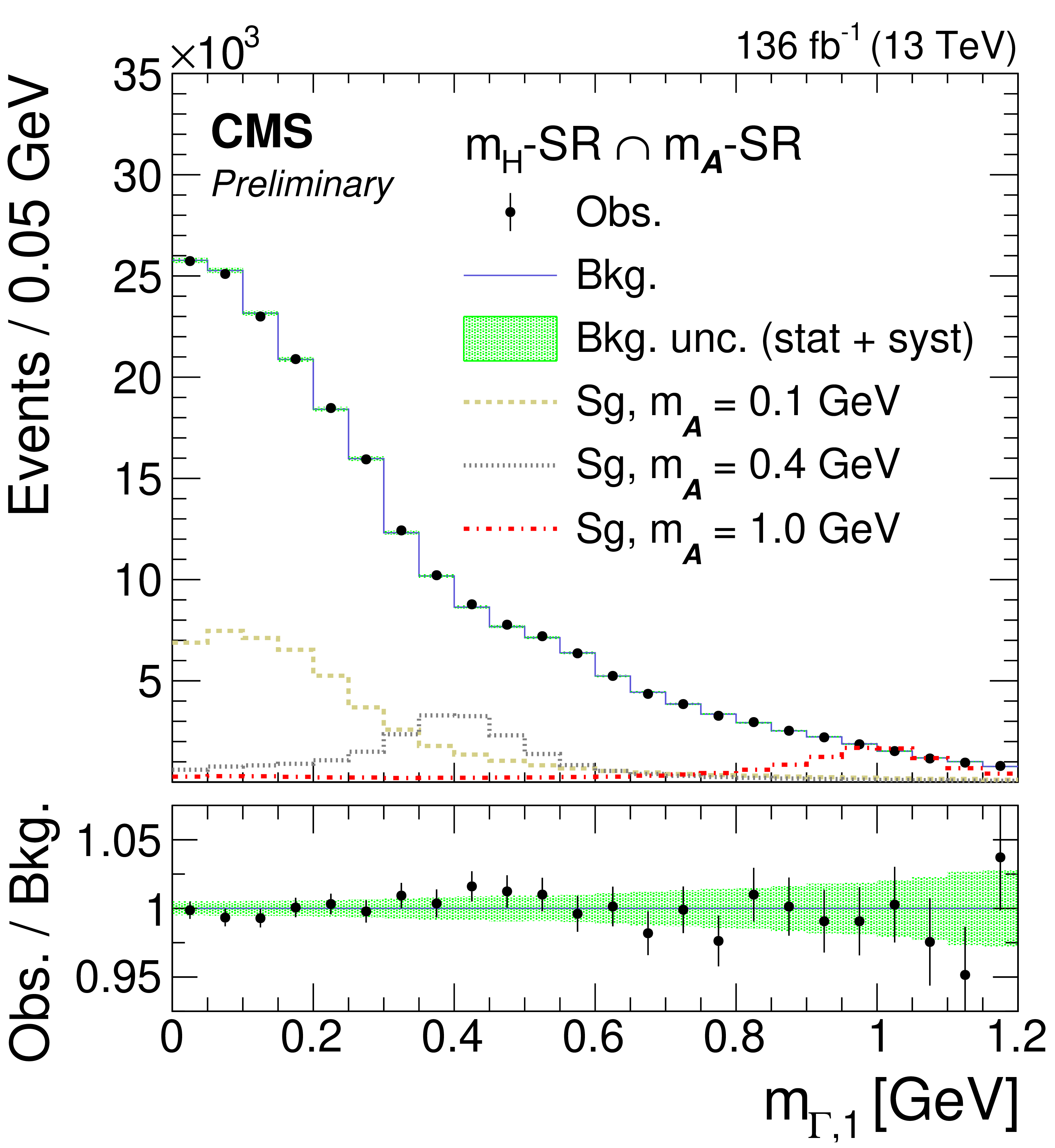
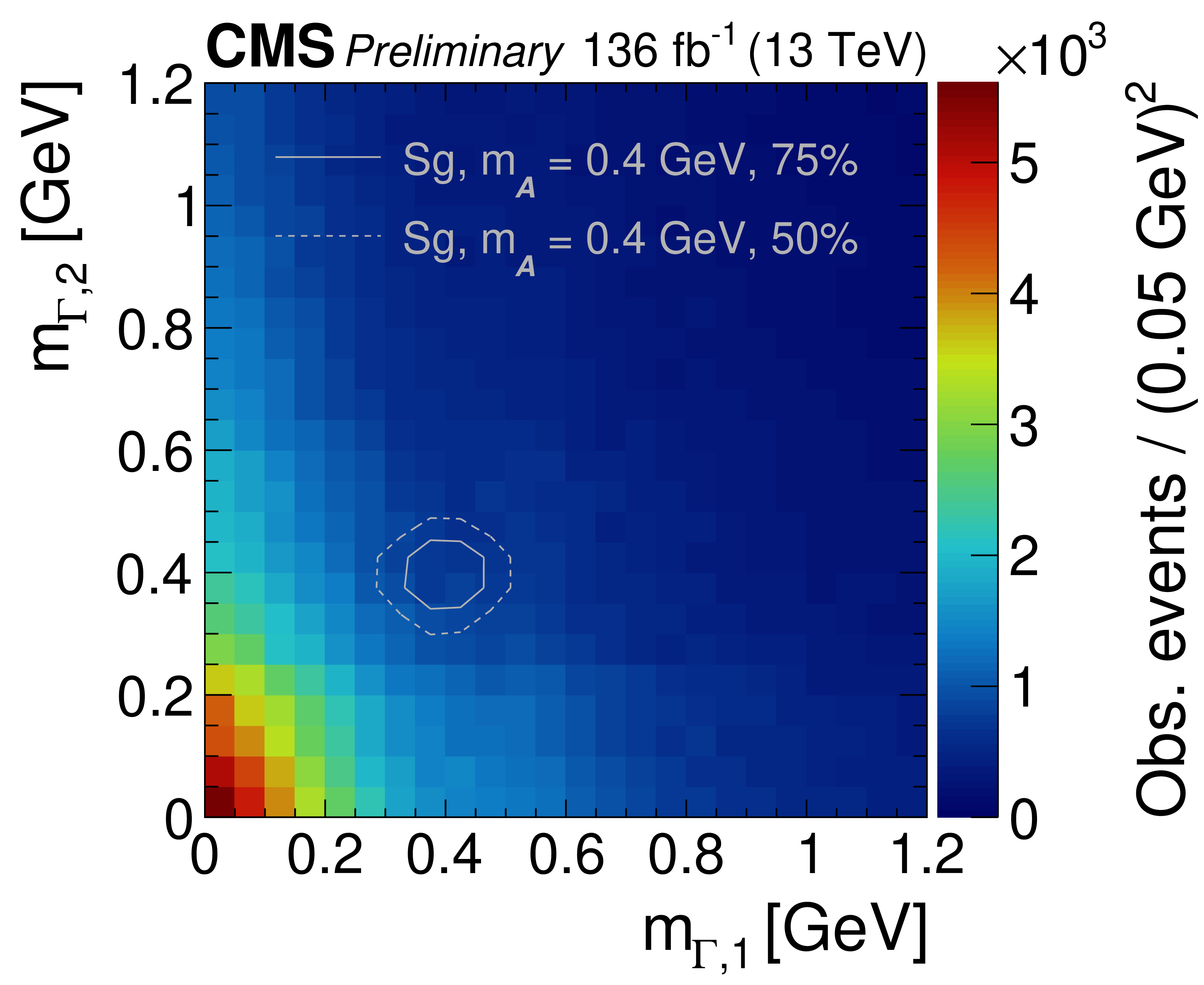
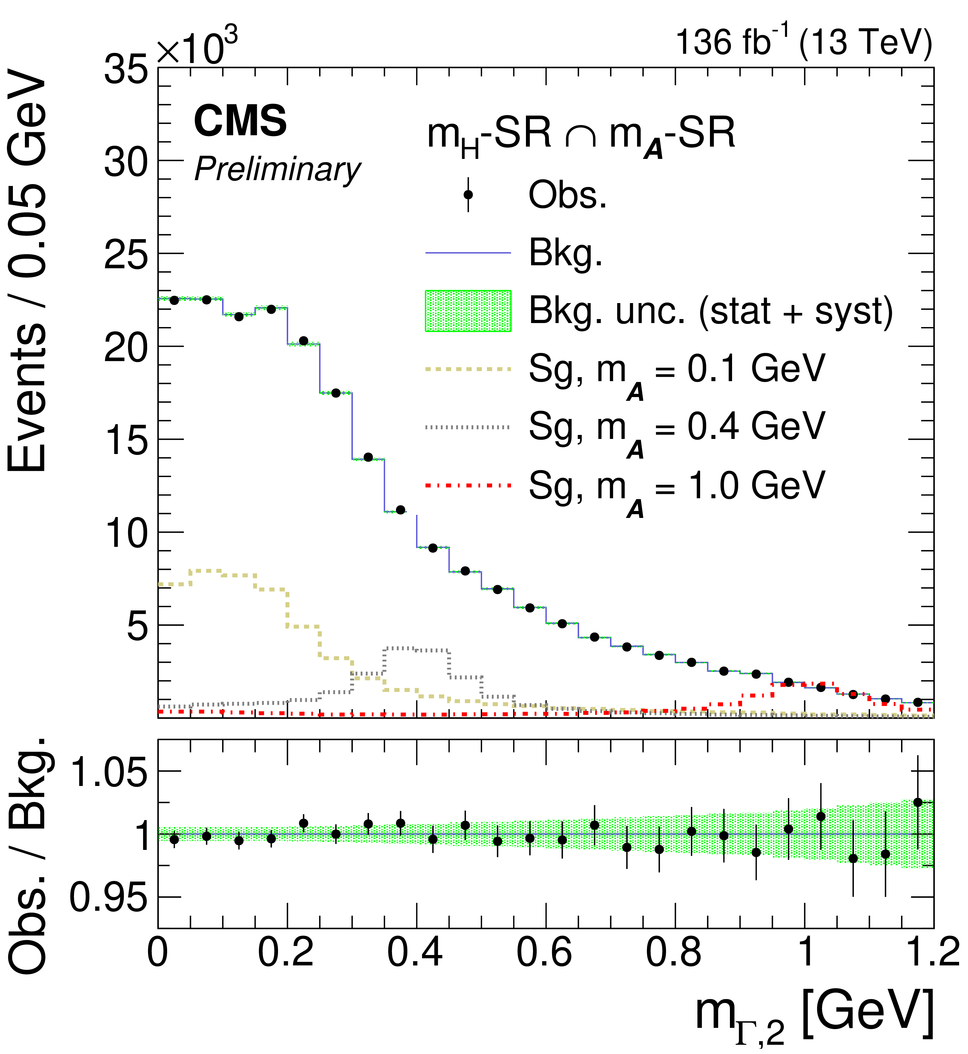
Observed mass distributions from signal candidate events. Center: the observed $m_{\Gamma,1}$ vs. $m_{\Gamma,2}$ 2D plot for candidate events in the $m_{\mathrm{H}}$-SR region. The color scale on the right of the plot gives the number of events per bin. The contours of simulated $\mathrm{H} \rightarrow {\mathcal {A}} {\mathcal {A}} \rightarrow 4\gamma $ events for $m_{{\mathcal {A}}} = $ 0.4 GeV are plotted at 75% (dashed contour) and $50%$ (dotted contour) of their maximum. The corresponding $m_{\Gamma,1}$ and $m_{\Gamma,2}$ projections for the overlap of the $m_{\mathrm{H}}$-SR and $m_{{\mathcal {A}}}$-SR regions are shown in the left and right figures, respectively. The observed distributions are given by the black points and the predicted background distributions by the blue curves. The vertical bars on the points represent the statistical uncertainties in the data, and the green bands show the total uncertainties in the background predictions. The spectra of simulated $\mathrm{H} \rightarrow {\mathcal {A}} {\mathcal {A}} \rightarrow 4\gamma $ events for $m_{{\mathcal {A}}}=$ 0.1 (yellow dashed curve), 0.4 (gray dotted curve), and 1.0 GeV (red dash-dotted curve) normalized to their respective expected upper limits times 10$^3$ are also provided. The lower panels give the ratios of the observed to the predicted distributions, with the green bands representing the total uncertainty in the ratios. |
png pdf |
Figure 2-a:
Observed mass distributions from signal candidate events. Center: the observed $m_{\Gamma,1}$ vs. $m_{\Gamma,2}$ 2D plot for candidate events in the $m_{\mathrm{H}}$-SR region. The color scale on the right of the plot gives the number of events per bin. The contours of simulated $\mathrm{H} \rightarrow {\mathcal {A}} {\mathcal {A}} \rightarrow 4\gamma $ events for $m_{{\mathcal {A}}} = $ 0.4 GeV are plotted at 75% (dashed contour) and $50%$ (dotted contour) of their maximum. The corresponding $m_{\Gamma,1}$ and $m_{\Gamma,2}$ projections for the overlap of the $m_{\mathrm{H}}$-SR and $m_{{\mathcal {A}}}$-SR regions are shown in the left and right figures, respectively. The observed distributions are given by the black points and the predicted background distributions by the blue curves. The vertical bars on the points represent the statistical uncertainties in the data, and the green bands show the total uncertainties in the background predictions. The spectra of simulated $\mathrm{H} \rightarrow {\mathcal {A}} {\mathcal {A}} \rightarrow 4\gamma $ events for $m_{{\mathcal {A}}}=$ 0.1 (yellow dashed curve), 0.4 (gray dotted curve), and 1.0 GeV (red dash-dotted curve) normalized to their respective expected upper limits times 10$^3$ are also provided. The lower panels give the ratios of the observed to the predicted distributions, with the green bands representing the total uncertainty in the ratios. |
png pdf |
Figure 2-b:
Observed mass distributions from signal candidate events. Center: the observed $m_{\Gamma,1}$ vs. $m_{\Gamma,2}$ 2D plot for candidate events in the $m_{\mathrm{H}}$-SR region. The color scale on the right of the plot gives the number of events per bin. The contours of simulated $\mathrm{H} \rightarrow {\mathcal {A}} {\mathcal {A}} \rightarrow 4\gamma $ events for $m_{{\mathcal {A}}} = $ 0.4 GeV are plotted at 75% (dashed contour) and $50%$ (dotted contour) of their maximum. The corresponding $m_{\Gamma,1}$ and $m_{\Gamma,2}$ projections for the overlap of the $m_{\mathrm{H}}$-SR and $m_{{\mathcal {A}}}$-SR regions are shown in the left and right figures, respectively. The observed distributions are given by the black points and the predicted background distributions by the blue curves. The vertical bars on the points represent the statistical uncertainties in the data, and the green bands show the total uncertainties in the background predictions. The spectra of simulated $\mathrm{H} \rightarrow {\mathcal {A}} {\mathcal {A}} \rightarrow 4\gamma $ events for $m_{{\mathcal {A}}}=$ 0.1 (yellow dashed curve), 0.4 (gray dotted curve), and 1.0 GeV (red dash-dotted curve) normalized to their respective expected upper limits times 10$^3$ are also provided. The lower panels give the ratios of the observed to the predicted distributions, with the green bands representing the total uncertainty in the ratios. |
png pdf |
Figure 2-c:
Observed mass distributions from signal candidate events. Center: the observed $m_{\Gamma,1}$ vs. $m_{\Gamma,2}$ 2D plot for candidate events in the $m_{\mathrm{H}}$-SR region. The color scale on the right of the plot gives the number of events per bin. The contours of simulated $\mathrm{H} \rightarrow {\mathcal {A}} {\mathcal {A}} \rightarrow 4\gamma $ events for $m_{{\mathcal {A}}} = $ 0.4 GeV are plotted at 75% (dashed contour) and $50%$ (dotted contour) of their maximum. The corresponding $m_{\Gamma,1}$ and $m_{\Gamma,2}$ projections for the overlap of the $m_{\mathrm{H}}$-SR and $m_{{\mathcal {A}}}$-SR regions are shown in the left and right figures, respectively. The observed distributions are given by the black points and the predicted background distributions by the blue curves. The vertical bars on the points represent the statistical uncertainties in the data, and the green bands show the total uncertainties in the background predictions. The spectra of simulated $\mathrm{H} \rightarrow {\mathcal {A}} {\mathcal {A}} \rightarrow 4\gamma $ events for $m_{{\mathcal {A}}}=$ 0.1 (yellow dashed curve), 0.4 (gray dotted curve), and 1.0 GeV (red dash-dotted curve) normalized to their respective expected upper limits times 10$^3$ are also provided. The lower panels give the ratios of the observed to the predicted distributions, with the green bands representing the total uncertainty in the ratios. |

png pdf |
Figure 3:
Observed (black solid curve with points) and median expected (blue dashed curve) 95% CL upper limits on $\mathcal {B}(\mathrm{H} \rightarrow {\mathcal {A}} {\mathcal {A}} \rightarrow 4\gamma)$ as a function of $m_{{\mathcal {A}}}$. The 68 and 95% CIs around the expected limits are shown by the green and yellow bands, respectively. The upper limit from a previous CMS measurement [1] of $\mathcal {B}(\mathrm{H} \rightarrow \gamma \gamma)$ is shown in red, where the width of the red band represents the uncertainty in the measurement. It is accurate for $m_{{\mathcal {A}}}\approx 0.1 GeV $ where the acceptance is comparable to that for the CMS SM $\mathrm{H} \rightarrow \gamma \gamma $ selection criteria and increases approximately twofold toward $m_{{\mathcal {A}}} = $ 1.0 GeV as the relative acceptance diverges. |

png pdf |
Figure A1:
Observed 2D-$m_{\Gamma}$ distribution from candidate events in the orthogonal, signal-depleted data sample in the $m_{\mathrm{H}}$-SR. The color scale on the right of the plot gives the number of events per bin. |
png pdf |
Figure A2:
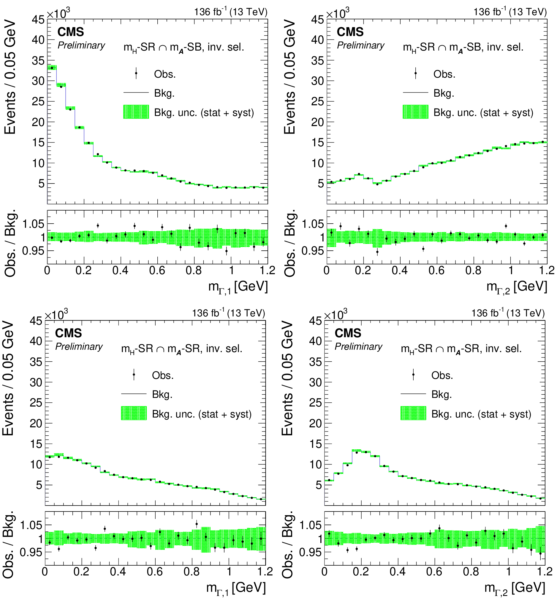
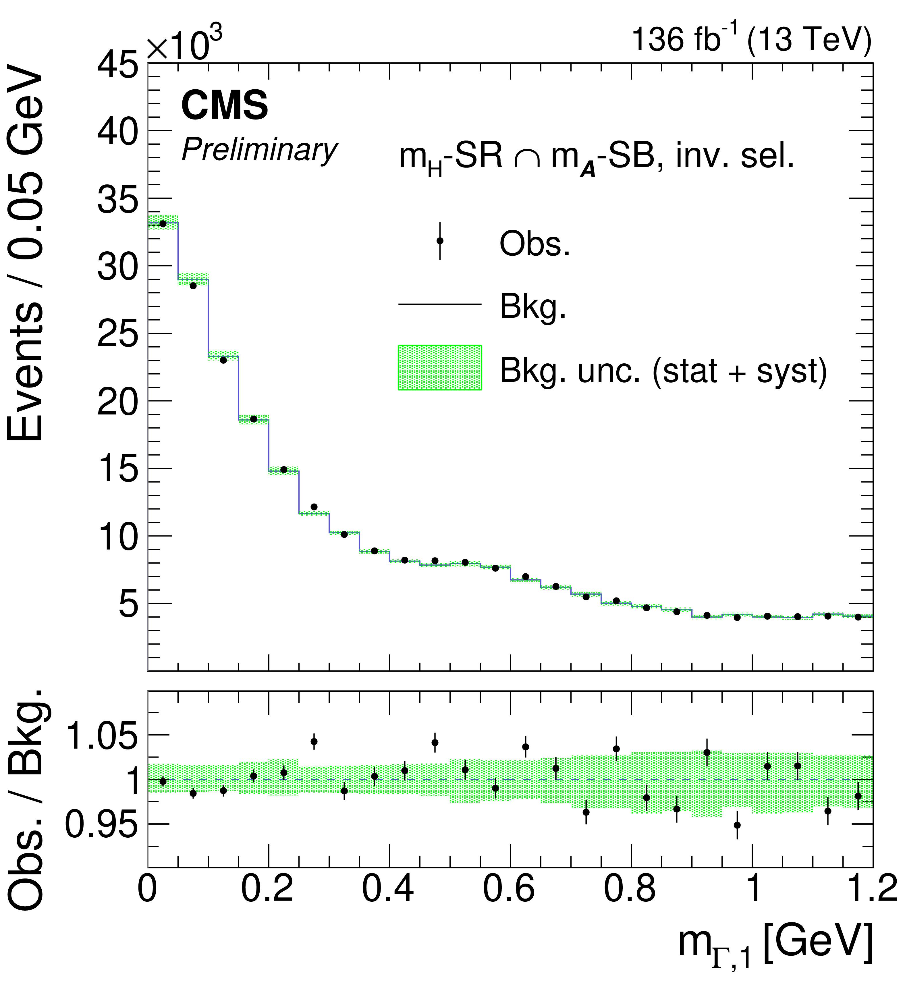
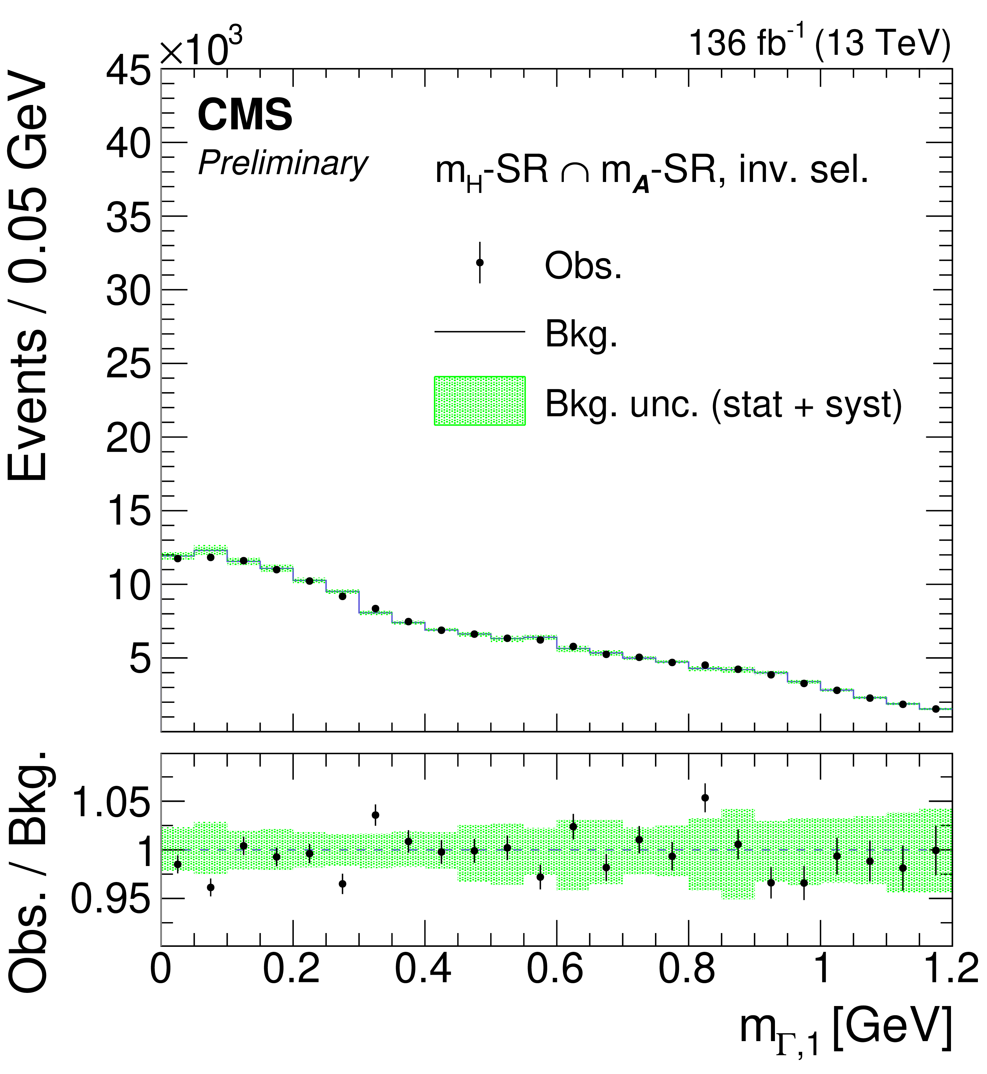
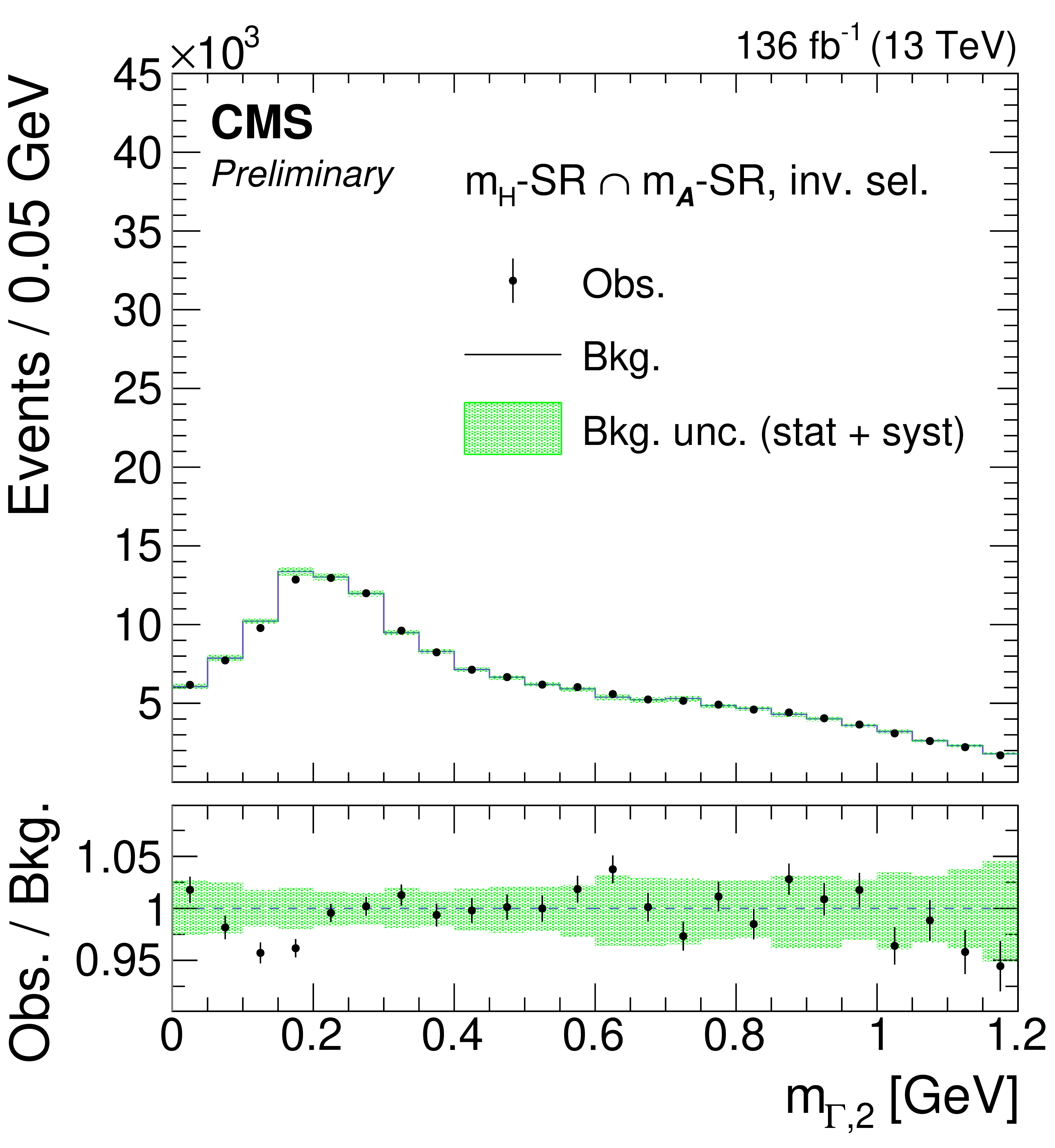
Observed vs. predicted $m_{\Gamma,1}$ (left) and $m_{\Gamma,2}$ (right) distributions in the $m_{{\mathcal {A}}}$-SB (upper) and $m_{{\mathcal {A}}}$-SR (lower) from candidate events in the orthogonal, signal-depleted data sample (inv. sel.) in the $m_{\mathrm{H}}$-SR. The observed distributions are given by the black points and the predicted background distributions by the blue curves. The vertical bars on the points represent the statistical uncertainties in the data, and the green bands show the total uncertainties in the background predictions. The lower panels give the ratios of the observed to the predicted distributions, with the green bands representing the total uncertainty in the ratios. |
png pdf |
Figure A2-a:
Observed vs. predicted $m_{\Gamma,1}$ (left) and $m_{\Gamma,2}$ (right) distributions in the $m_{{\mathcal {A}}}$-SB (upper) and $m_{{\mathcal {A}}}$-SR (lower) from candidate events in the orthogonal, signal-depleted data sample (inv. sel.) in the $m_{\mathrm{H}}$-SR. The observed distributions are given by the black points and the predicted background distributions by the blue curves. The vertical bars on the points represent the statistical uncertainties in the data, and the green bands show the total uncertainties in the background predictions. The lower panels give the ratios of the observed to the predicted distributions, with the green bands representing the total uncertainty in the ratios. |

png pdf |
Figure A2-b:
Observed vs. predicted $m_{\Gamma,1}$ (left) and $m_{\Gamma,2}$ (right) distributions in the $m_{{\mathcal {A}}}$-SB (upper) and $m_{{\mathcal {A}}}$-SR (lower) from candidate events in the orthogonal, signal-depleted data sample (inv. sel.) in the $m_{\mathrm{H}}$-SR. The observed distributions are given by the black points and the predicted background distributions by the blue curves. The vertical bars on the points represent the statistical uncertainties in the data, and the green bands show the total uncertainties in the background predictions. The lower panels give the ratios of the observed to the predicted distributions, with the green bands representing the total uncertainty in the ratios. |
png pdf |
Figure A2-c:
Observed vs. predicted $m_{\Gamma,1}$ (left) and $m_{\Gamma,2}$ (right) distributions in the $m_{{\mathcal {A}}}$-SB (upper) and $m_{{\mathcal {A}}}$-SR (lower) from candidate events in the orthogonal, signal-depleted data sample (inv. sel.) in the $m_{\mathrm{H}}$-SR. The observed distributions are given by the black points and the predicted background distributions by the blue curves. The vertical bars on the points represent the statistical uncertainties in the data, and the green bands show the total uncertainties in the background predictions. The lower panels give the ratios of the observed to the predicted distributions, with the green bands representing the total uncertainty in the ratios. |
png pdf |
Figure A2-d:
Observed vs. predicted $m_{\Gamma,1}$ (left) and $m_{\Gamma,2}$ (right) distributions in the $m_{{\mathcal {A}}}$-SB (upper) and $m_{{\mathcal {A}}}$-SR (lower) from candidate events in the orthogonal, signal-depleted data sample (inv. sel.) in the $m_{\mathrm{H}}$-SR. The observed distributions are given by the black points and the predicted background distributions by the blue curves. The vertical bars on the points represent the statistical uncertainties in the data, and the green bands show the total uncertainties in the background predictions. The lower panels give the ratios of the observed to the predicted distributions, with the green bands representing the total uncertainty in the ratios. |
png pdf |
Figure A3:
Predicted 2D-$m_{\Gamma}$ distribution for signal candidate events in the $m_{\mathrm{H}}$-SR. The color scale on the right of the plot gives the number of events per bin. |
png pdf |
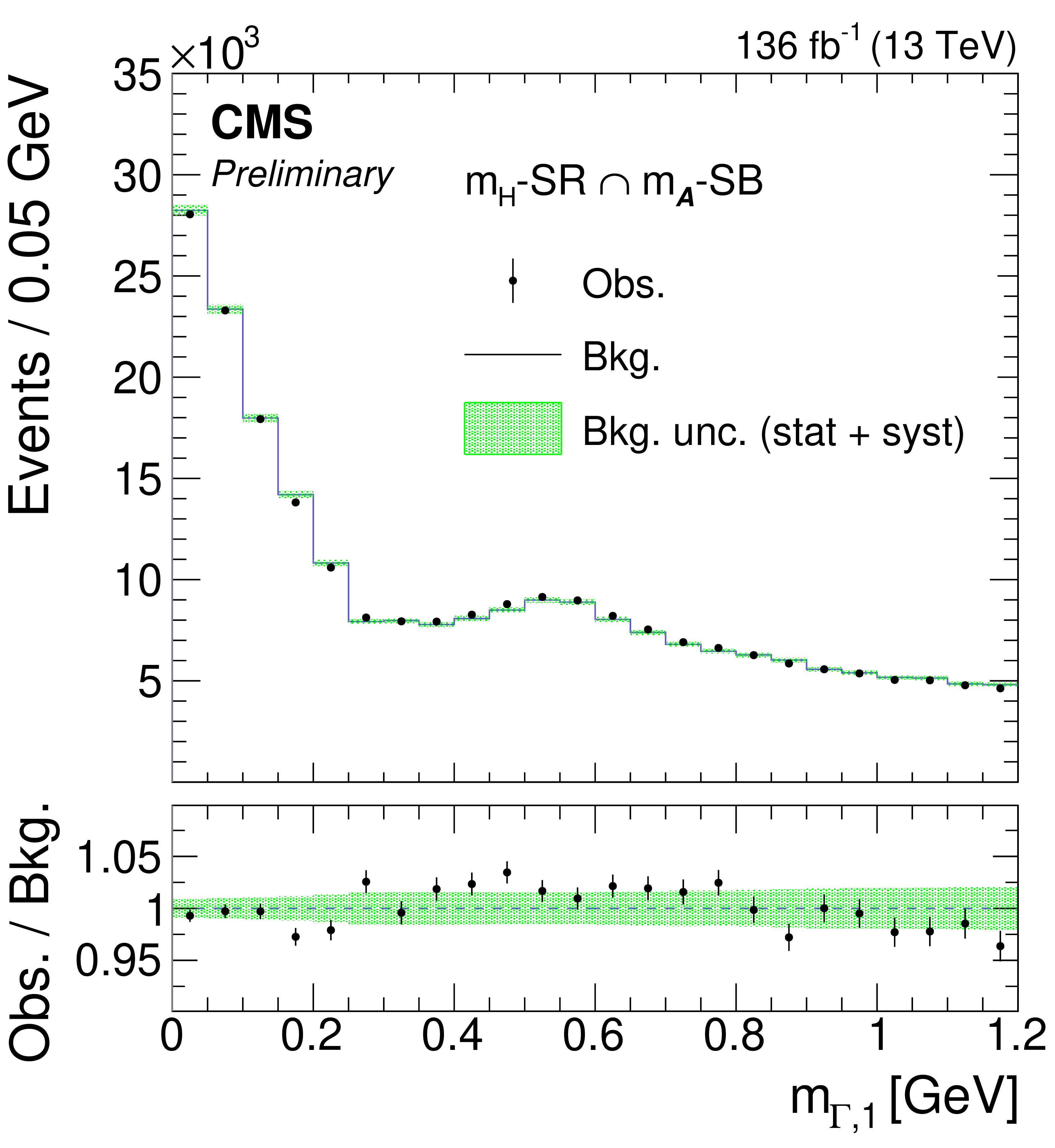
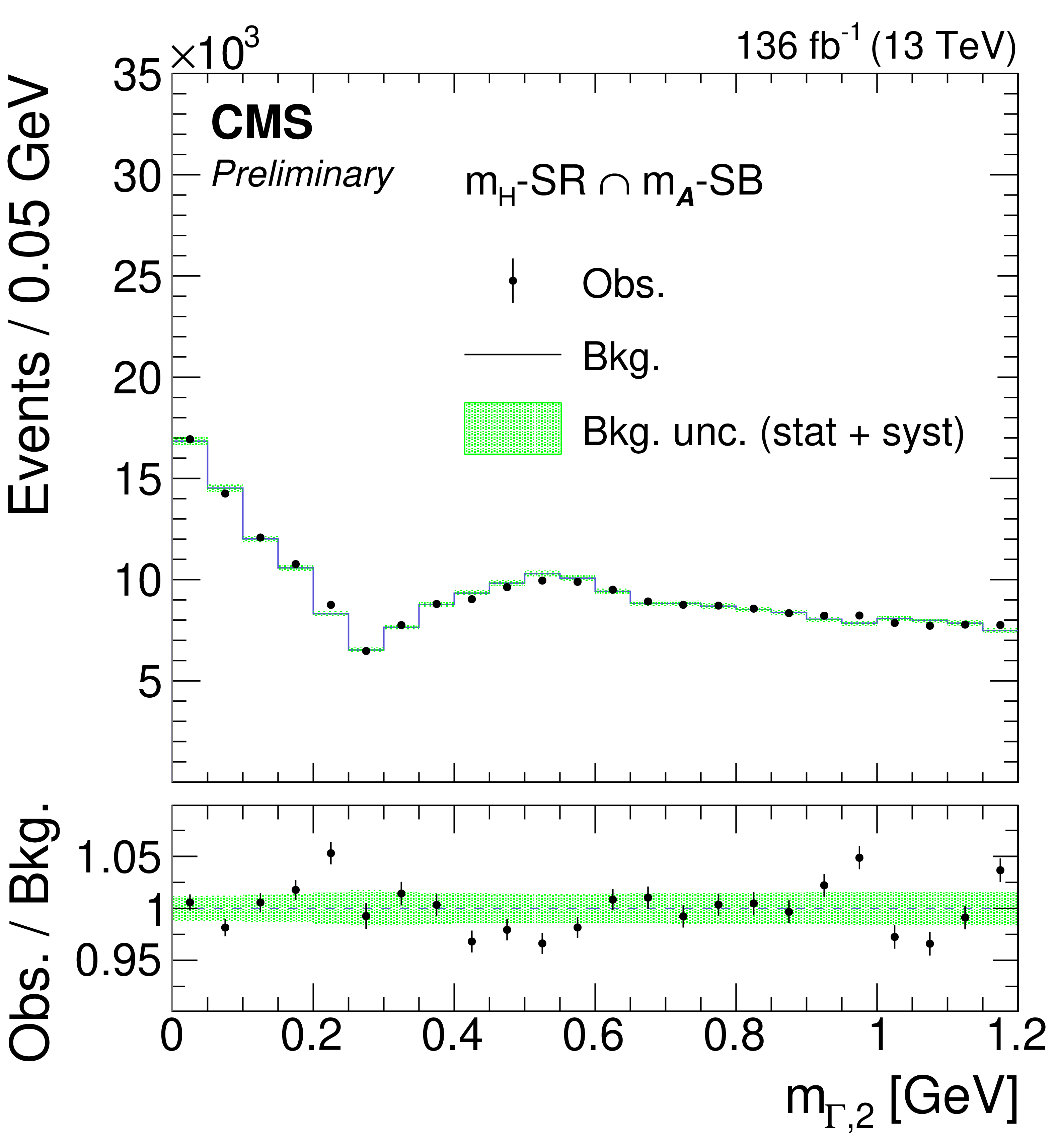
Figure A4:
Observed vs. predicted $m_{\Gamma,1}$ (left) and $m_{\Gamma,2}$ (right) distributions in the $m_{{\mathcal {A}}}$-SB from signal candidates events in the $m_{\mathrm{H}}$-SR. The observed distributions are given by the black points and the predicted background distributions by the blue curves. The vertical bars on the points represent the statistical uncertainties in the data, and the green bands show the total uncertainties in the background predictions. The lower panels give the ratios of the observed to the predicted distributions, with the green bands representing the total uncertainty in the ratios. |
png pdf |
Figure A4-a:
Observed vs. predicted $m_{\Gamma,1}$ (left) and $m_{\Gamma,2}$ (right) distributions in the $m_{{\mathcal {A}}}$-SB from signal candidates events in the $m_{\mathrm{H}}$-SR. The observed distributions are given by the black points and the predicted background distributions by the blue curves. The vertical bars on the points represent the statistical uncertainties in the data, and the green bands show the total uncertainties in the background predictions. The lower panels give the ratios of the observed to the predicted distributions, with the green bands representing the total uncertainty in the ratios. |
png pdf |
Figure A4-b:
Observed vs. predicted $m_{\Gamma,1}$ (left) and $m_{\Gamma,2}$ (right) distributions in the $m_{{\mathcal {A}}}$-SB from signal candidates events in the $m_{\mathrm{H}}$-SR. The observed distributions are given by the black points and the predicted background distributions by the blue curves. The vertical bars on the points represent the statistical uncertainties in the data, and the green bands show the total uncertainties in the background predictions. The lower panels give the ratios of the observed to the predicted distributions, with the green bands representing the total uncertainty in the ratios. |
| Summary |
| In summary, results of a search for the exotic Higgs boson decay H $ \rightarrow \mathcal{A}\mathcal{A} \rightarrow 4\gamma$ have been presented. Events reconstructed with two photons are used, where each photon is assumed to be a misreconstructed, merged $\mathcal{A} \rightarrow \gamma\gamma$ candidate. The first direct probe of the invariant mass spectrum of merged $\mathcal{A} \rightarrow \gamma\gamma$ candidates is performed to discriminate potential signal events from the SM background. No excess of events above the estimated background is found. Upper limits on the branching fraction $\mathcal{B}(\mathrm{H} \rightarrow \mathcal{A}\mathcal{A} \rightarrow 4\gamma)$ of 0.9--3.3$\times$10$^{-3}$ are set at the 95% confidence level for masses of $\mathcal{A}$ in the range 0.1 $ < m_{\mathcal{A}} < $ 1.2 GeV, assuming prompt $\mathcal{A}$ decays. |
| References | ||||
| 1 | CMS Collaboration | Combined measurements of Higgs boson couplings in proton-proton collisions at $ \sqrt{s}= $ 13 TeV | EPJC 79 (2019) 421 | CMS-HIG-17-031 1809.10733 |
| 2 | D. Curtin et al. | Exotic decays of the 125 GeV Higgs boson | PRD 90 (2014) 075004 | 1312.4992 |
| 3 | D. Curtin, R. Essig, S. Gori, and J. Shelton | Illuminating dark photons with high-energy colliders | JHEP 02 (2015) 157 | 1412.0018 |
| 4 | R. D. Peccei and H. R. Quinn | $ \mathrm{CP} $ conservation in the presence of pseudoparticles | PRL 38 (1977) 1440 | |
| 5 | M. Bauer, M. Neubert, and A. Thamm | Collider probes of axion-like particles | JHEP 12 (2017) 044 | 1708.00443 |
| 6 | R. D. Peccei | The strong CP problem and axions | in Axions, M. Kuster, G. Raffelt, and B. Beltran, eds Springer Berlin Heidelberg | hep-ph/0607268 |
| 7 | CMS Collaboration | Search for an exotic decay of the Higgs boson to a pair of light pseudoscalars in the final state of two muons and two $ \tau $ leptons in proton-proton collisions at $ \sqrt{s}= $ 13 TeV | JHEP 11 (2018) 018 | CMS-HIG-17-029 1805.04865 |
| 8 | CMS Collaboration | A search for pair production of new light bosons decaying into muons in proton-proton collisions at 13 TeV | PLB 796 (2019) 131 | CMS-HIG-18-003 1812.00380 |
| 9 | CMS Collaboration | Search for light pseudoscalar boson pairs produced from decays of the 125 GeV Higgs boson in final states with two muons and two nearby tracks in pp collisions at $ \sqrt{s}= $ 13 TeV | PLB 800 (2020) 135087 | CMS-HIG-18-006 1907.07235 |
| 10 | CMS Collaboration | Search for an exotic decay of the Higgs boson to a pair of light pseudoscalars in the final state with two muons and two b quarks in pp collisions at 13 TeV | PLB 795 (2019) 398 | CMS-HIG-18-011 1812.06359 |
| 11 | CMS Collaboration | Search for a light pseudoscalar Higgs boson in the boosted $ \mu\mu\tau\tau $ final state in proton-proton collisions at $ \sqrt{s} = $ 13 TeV | JHEP 08 (2020) 139 | CMS-HIG-18-024 2005.08694 |
| 12 | B. A. Dobrescu, G. Landsberg, and K. T. Matchev | Higgs boson decays to $ \mathrm{CP} $-odd scalars at the Fermilab Tevatron and beyond | PRD 63 (2001) 075003 | hep-ph/0005308 |
| 13 | P. W. Graham et al. | Experimental searches for the axion and axion-like particles | Annu. Rev. Nucl. Part. Sci. 65 (2015) 485 | 1602.00039 |
| 14 | I. G. Irastorza and J. Redondo | New experimental approaches in the search for axion-like particles | Prog. Part. NP 102 (2018) 89 | 1801.08127 |
| 15 | Particle Data Group Collaboration | Review of particle physics | PTEP 2020 (2020) 083C01 | |
| 16 | GlueX Collaboration | Search for photoproduction of axion-like particles at GlueX | 2021 | 2109.13439 |
| 17 | S. Knapen, T. Lin, H. K. Lou, and T. Melia | Searching for axionlike particles with ultraperipheral heavy-ion collisions | PRL 118 (2017) 171801 | 1607.06083 |
| 18 | G. G. Raffelt | Astrophysical axion bounds | in Axions, M. Kuster, G. Raffelt, and B. Beltran, eds Springer Berlin Heidelberg | hep-ph/0611350 |
| 19 | P. Sikivie | Axion cosmology | in Axions, M. Kuster, G. Raffelt, and B. Beltran, eds Springer Berlin Heidelberg | astro-ph/0610440 |
| 20 | D. J. E. Marsh | Axion cosmology | Phys. Rep. 643 (2016) 1 | 1510.07633 |
| 21 | F. Chadha-Day, J. Ellis, and D. J. E. Marsh | Axion dark matter: What is it and why now? | 2021 | 2105.01406 |
| 22 | ATLAS Collaboration | Search for a Higgs boson decaying to four photons through light $ \mathrm{CP} $-odd scalar coupling using 4.9 fb$^{-1}$ of 7 TeV pp collision data taken with ATLAS detector at the LHC | ATLAS-CONF-2012-079 | |
|
|
Compact Muon Solenoid LHC, CERN |
|

|

|

|

|

|