

Compact Muon Solenoid
LHC, CERN
| CMS-PAS-EXO-19-021 | ||
| Search for long-lived particles decaying into displaced jets | ||
| CMS Collaboration | ||
| May 2020 | ||
| Abstract: An inclusive search for long-lived particles decaying into jets is presented. The search uses a data sample corresponding to an integrated luminosity of 132 fb$^{-1}$ from proton-proton collisions at a center-of-mass energy of 13 TeV, collected with the CMS detector at the LHC in 2016, 2017, and 2018. The analysis examines the distinctive topology of displaced tracks and displaced vertices within a dijet system. For a simplified model, where pair-produced long-lived neutral particles decay into quark-antiquark pairs, pair production cross sections larger than 0.07 fb are excluded at 95% confidence level for long-lived particle masses larger than 500 GeV and mean proper decay lengths between 2 and 250 mm. For a model where the standard model Higgs boson decays to two long-lived scalars and then each scalar decays to a quark-antiquark pair, branching fractions larger than 1% can be excluded for mean proper decay lengths between 1 mm and 1 m. A group of supersymmetry models with pair-produced long-lived gluinos or top squarks decaying into different final-state topologies containing displaced jets is also tested. Gluino masses up to 2500 GeV and top squark masses up to 1600 GeV are excluded for mean proper decay lengths between 3 and 300 mm. The best mass bounds reach 2600 GeV for long-lived gluinos and 1800 GeV for long-lived top squarks. These are currently the most restrictive limits on these models. | ||
|
Links:
CDS record (PDF) ;
CADI line (restricted) ;
These preliminary results are superseded in this paper, Accepted by PRD. The superseded preliminary plots can be found here. |
||
| Figures | |
png pdf |
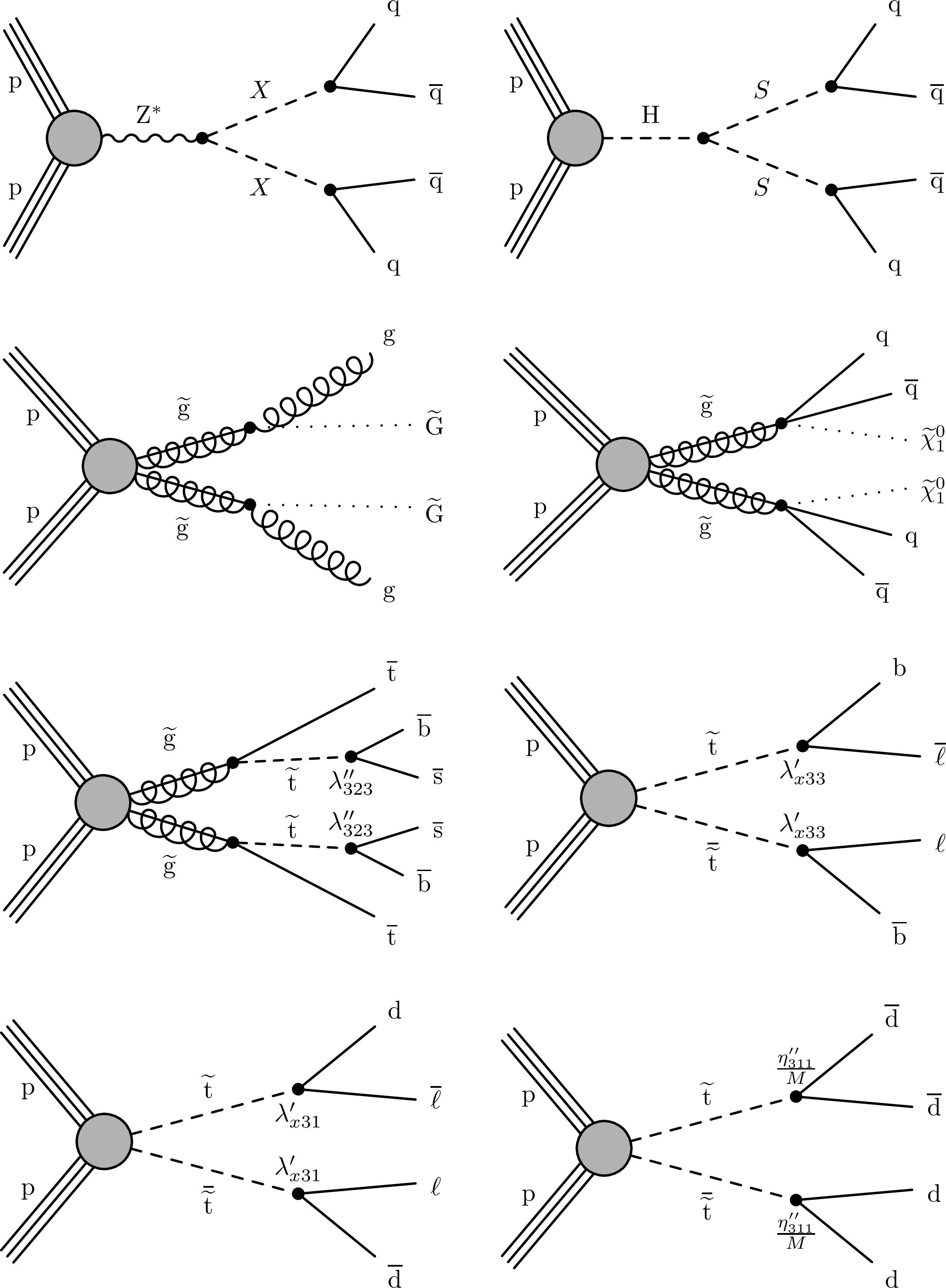
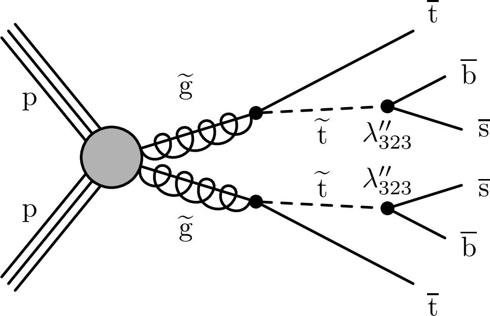
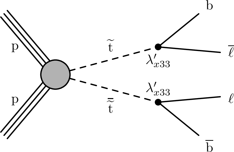
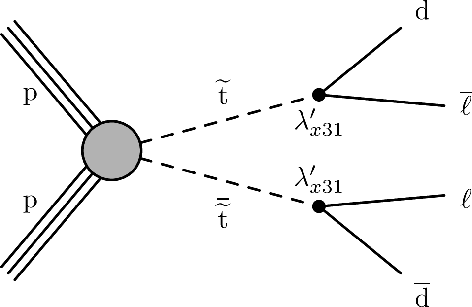
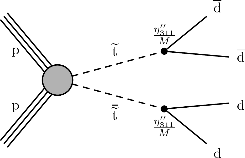
Figure 1:
The Feynman diagrams for different long-lived models considered, including jet-jet model (upper left), exotic decay of the SM Higgs boson (upper right), general gauge mediation with ${\mathrm{\tilde{g}}} \to \mathrm{g} \tilde{\mathrm{G}} $ decay (the second row, left), mini-split SUSY with ${\mathrm{\tilde{g}}} \to \mathrm{q} \mathrm{\bar{q}} \tilde{\chi}^{0}_{1}$ decay (the second row, right), RPV SUSY with ${\mathrm{\tilde{g}}} \to \mathrm{t} \mathrm{b} \mathrm{s} $ decay (the third row, left), RPV SUSY with $\tilde{\mathrm{t}} \to \mathrm{b} \ell $ decay (the third row, right), RPV SUSY with $\tilde{\mathrm{t}} \to \mathrm{d} \ell $ decay, and dynamical RPV SUSY with $\tilde{\mathrm{t}} \to \mathrm{\bar{d}} \mathrm{\bar{d}} $ decay (lower right). |
png pdf |
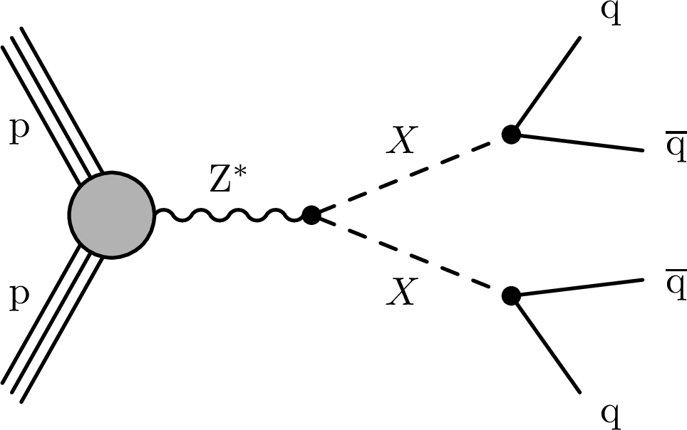
Figure 1-a:
The Feynman diagrams for different long-lived models considered, including jet-jet model (upper left), exotic decay of the SM Higgs boson (upper right), general gauge mediation with ${\mathrm{\tilde{g}}} \to \mathrm{g} \tilde{\mathrm{G}} $ decay (the second row, left), mini-split SUSY with ${\mathrm{\tilde{g}}} \to \mathrm{q} \mathrm{\bar{q}} \tilde{\chi}^{0}_{1}$ decay (the second row, right), RPV SUSY with ${\mathrm{\tilde{g}}} \to \mathrm{t} \mathrm{b} \mathrm{s} $ decay (the third row, left), RPV SUSY with $\tilde{\mathrm{t}} \to \mathrm{b} \ell $ decay (the third row, right), RPV SUSY with $\tilde{\mathrm{t}} \to \mathrm{d} \ell $ decay, and dynamical RPV SUSY with $\tilde{\mathrm{t}} \to \mathrm{\bar{d}} \mathrm{\bar{d}} $ decay (lower right). |

png pdf |
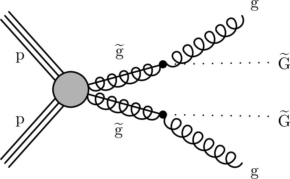
Figure 1-b:
The Feynman diagrams for different long-lived models considered, including jet-jet model (upper left), exotic decay of the SM Higgs boson (upper right), general gauge mediation with ${\mathrm{\tilde{g}}} \to \mathrm{g} \tilde{\mathrm{G}} $ decay (the second row, left), mini-split SUSY with ${\mathrm{\tilde{g}}} \to \mathrm{q} \mathrm{\bar{q}} \tilde{\chi}^{0}_{1}$ decay (the second row, right), RPV SUSY with ${\mathrm{\tilde{g}}} \to \mathrm{t} \mathrm{b} \mathrm{s} $ decay (the third row, left), RPV SUSY with $\tilde{\mathrm{t}} \to \mathrm{b} \ell $ decay (the third row, right), RPV SUSY with $\tilde{\mathrm{t}} \to \mathrm{d} \ell $ decay, and dynamical RPV SUSY with $\tilde{\mathrm{t}} \to \mathrm{\bar{d}} \mathrm{\bar{d}} $ decay (lower right). |
png pdf |
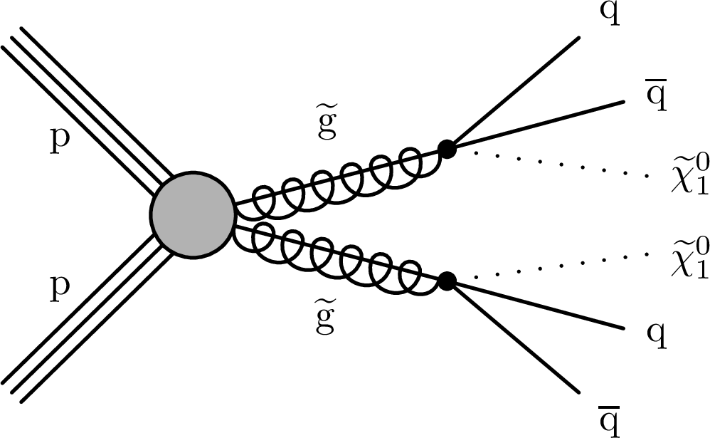
Figure 1-c:
The Feynman diagrams for different long-lived models considered, including jet-jet model (upper left), exotic decay of the SM Higgs boson (upper right), general gauge mediation with ${\mathrm{\tilde{g}}} \to \mathrm{g} \tilde{\mathrm{G}} $ decay (the second row, left), mini-split SUSY with ${\mathrm{\tilde{g}}} \to \mathrm{q} \mathrm{\bar{q}} \tilde{\chi}^{0}_{1}$ decay (the second row, right), RPV SUSY with ${\mathrm{\tilde{g}}} \to \mathrm{t} \mathrm{b} \mathrm{s} $ decay (the third row, left), RPV SUSY with $\tilde{\mathrm{t}} \to \mathrm{b} \ell $ decay (the third row, right), RPV SUSY with $\tilde{\mathrm{t}} \to \mathrm{d} \ell $ decay, and dynamical RPV SUSY with $\tilde{\mathrm{t}} \to \mathrm{\bar{d}} \mathrm{\bar{d}} $ decay (lower right). |
png pdf |
Figure 1-d:
The Feynman diagrams for different long-lived models considered, including jet-jet model (upper left), exotic decay of the SM Higgs boson (upper right), general gauge mediation with ${\mathrm{\tilde{g}}} \to \mathrm{g} \tilde{\mathrm{G}} $ decay (the second row, left), mini-split SUSY with ${\mathrm{\tilde{g}}} \to \mathrm{q} \mathrm{\bar{q}} \tilde{\chi}^{0}_{1}$ decay (the second row, right), RPV SUSY with ${\mathrm{\tilde{g}}} \to \mathrm{t} \mathrm{b} \mathrm{s} $ decay (the third row, left), RPV SUSY with $\tilde{\mathrm{t}} \to \mathrm{b} \ell $ decay (the third row, right), RPV SUSY with $\tilde{\mathrm{t}} \to \mathrm{d} \ell $ decay, and dynamical RPV SUSY with $\tilde{\mathrm{t}} \to \mathrm{\bar{d}} \mathrm{\bar{d}} $ decay (lower right). |
png pdf |
Figure 1-e:
The Feynman diagrams for different long-lived models considered, including jet-jet model (upper left), exotic decay of the SM Higgs boson (upper right), general gauge mediation with ${\mathrm{\tilde{g}}} \to \mathrm{g} \tilde{\mathrm{G}} $ decay (the second row, left), mini-split SUSY with ${\mathrm{\tilde{g}}} \to \mathrm{q} \mathrm{\bar{q}} \tilde{\chi}^{0}_{1}$ decay (the second row, right), RPV SUSY with ${\mathrm{\tilde{g}}} \to \mathrm{t} \mathrm{b} \mathrm{s} $ decay (the third row, left), RPV SUSY with $\tilde{\mathrm{t}} \to \mathrm{b} \ell $ decay (the third row, right), RPV SUSY with $\tilde{\mathrm{t}} \to \mathrm{d} \ell $ decay, and dynamical RPV SUSY with $\tilde{\mathrm{t}} \to \mathrm{\bar{d}} \mathrm{\bar{d}} $ decay (lower right). |
png pdf |
Figure 1-f:
The Feynman diagrams for different long-lived models considered, including jet-jet model (upper left), exotic decay of the SM Higgs boson (upper right), general gauge mediation with ${\mathrm{\tilde{g}}} \to \mathrm{g} \tilde{\mathrm{G}} $ decay (the second row, left), mini-split SUSY with ${\mathrm{\tilde{g}}} \to \mathrm{q} \mathrm{\bar{q}} \tilde{\chi}^{0}_{1}$ decay (the second row, right), RPV SUSY with ${\mathrm{\tilde{g}}} \to \mathrm{t} \mathrm{b} \mathrm{s} $ decay (the third row, left), RPV SUSY with $\tilde{\mathrm{t}} \to \mathrm{b} \ell $ decay (the third row, right), RPV SUSY with $\tilde{\mathrm{t}} \to \mathrm{d} \ell $ decay, and dynamical RPV SUSY with $\tilde{\mathrm{t}} \to \mathrm{\bar{d}} \mathrm{\bar{d}} $ decay (lower right). |
png pdf |
Figure 1-g:
The Feynman diagrams for different long-lived models considered, including jet-jet model (upper left), exotic decay of the SM Higgs boson (upper right), general gauge mediation with ${\mathrm{\tilde{g}}} \to \mathrm{g} \tilde{\mathrm{G}} $ decay (the second row, left), mini-split SUSY with ${\mathrm{\tilde{g}}} \to \mathrm{q} \mathrm{\bar{q}} \tilde{\chi}^{0}_{1}$ decay (the second row, right), RPV SUSY with ${\mathrm{\tilde{g}}} \to \mathrm{t} \mathrm{b} \mathrm{s} $ decay (the third row, left), RPV SUSY with $\tilde{\mathrm{t}} \to \mathrm{b} \ell $ decay (the third row, right), RPV SUSY with $\tilde{\mathrm{t}} \to \mathrm{d} \ell $ decay, and dynamical RPV SUSY with $\tilde{\mathrm{t}} \to \mathrm{\bar{d}} \mathrm{\bar{d}} $ decay (lower right). |
png pdf |
Figure 1-h:
The Feynman diagrams for different long-lived models considered, including jet-jet model (upper left), exotic decay of the SM Higgs boson (upper right), general gauge mediation with ${\mathrm{\tilde{g}}} \to \mathrm{g} \tilde{\mathrm{G}} $ decay (the second row, left), mini-split SUSY with ${\mathrm{\tilde{g}}} \to \mathrm{q} \mathrm{\bar{q}} \tilde{\chi}^{0}_{1}$ decay (the second row, right), RPV SUSY with ${\mathrm{\tilde{g}}} \to \mathrm{t} \mathrm{b} \mathrm{s} $ decay (the third row, left), RPV SUSY with $\tilde{\mathrm{t}} \to \mathrm{b} \ell $ decay (the third row, right), RPV SUSY with $\tilde{\mathrm{t}} \to \mathrm{d} \ell $ decay, and dynamical RPV SUSY with $\tilde{\mathrm{t}} \to \mathrm{\bar{d}} \mathrm{\bar{d}} $ decay (lower right). |
png pdf |
Figure 2:
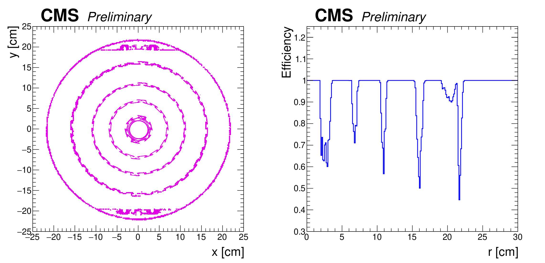
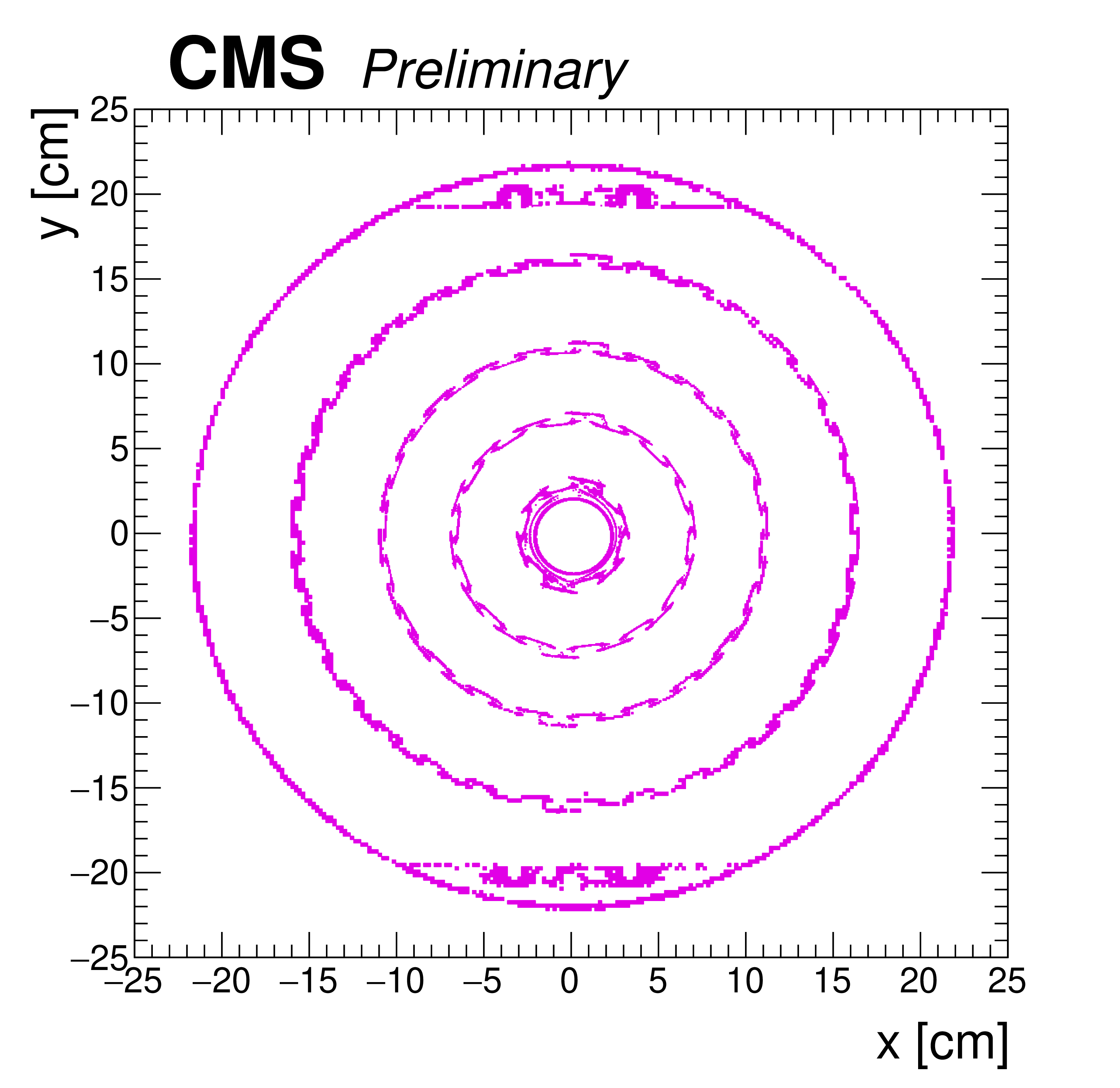
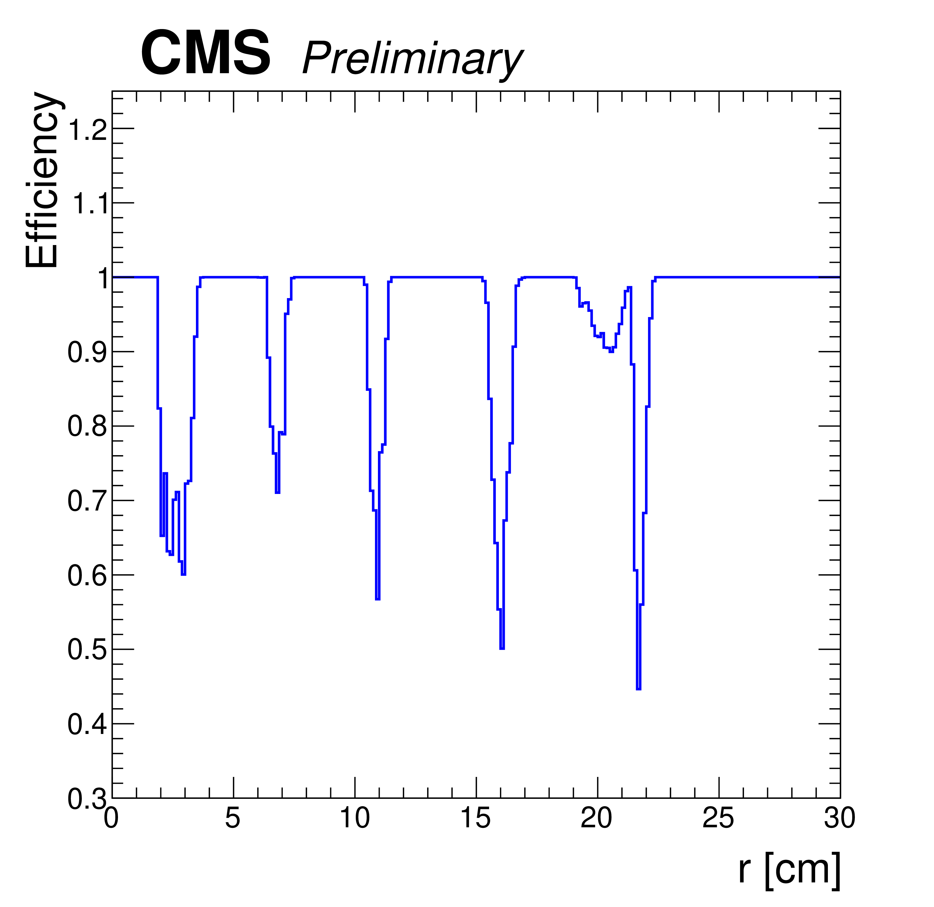
Left: the NI-veto map based on NI vertex reconstruction in the 2017 and 2018 data collected by the CMS detector, corresponding to the geometry of the Phase I CMS pixel detector [77]. The structures of different pixel layers can be clearly seen. Right: the efficiency for a given vertex candidate to pass the NI-veto as a function of radius $r$ ($r=\sqrt {x^{2}+y^{2}})$. |
png pdf |
Figure 2-a:
Left: the NI-veto map based on NI vertex reconstruction in the 2017 and 2018 data collected by the CMS detector, corresponding to the geometry of the Phase I CMS pixel detector [77]. The structures of different pixel layers can be clearly seen. Right: the efficiency for a given vertex candidate to pass the NI-veto as a function of radius $r$ ($r=\sqrt {x^{2}+y^{2}})$. |
png pdf |
Figure 2-b:
Left: the NI-veto map based on NI vertex reconstruction in the 2017 and 2018 data collected by the CMS detector, corresponding to the geometry of the Phase I CMS pixel detector [77]. The structures of different pixel layers can be clearly seen. Right: the efficiency for a given vertex candidate to pass the NI-veto as a function of radius $r$ ($r=\sqrt {x^{2}+y^{2}})$. |
png pdf |
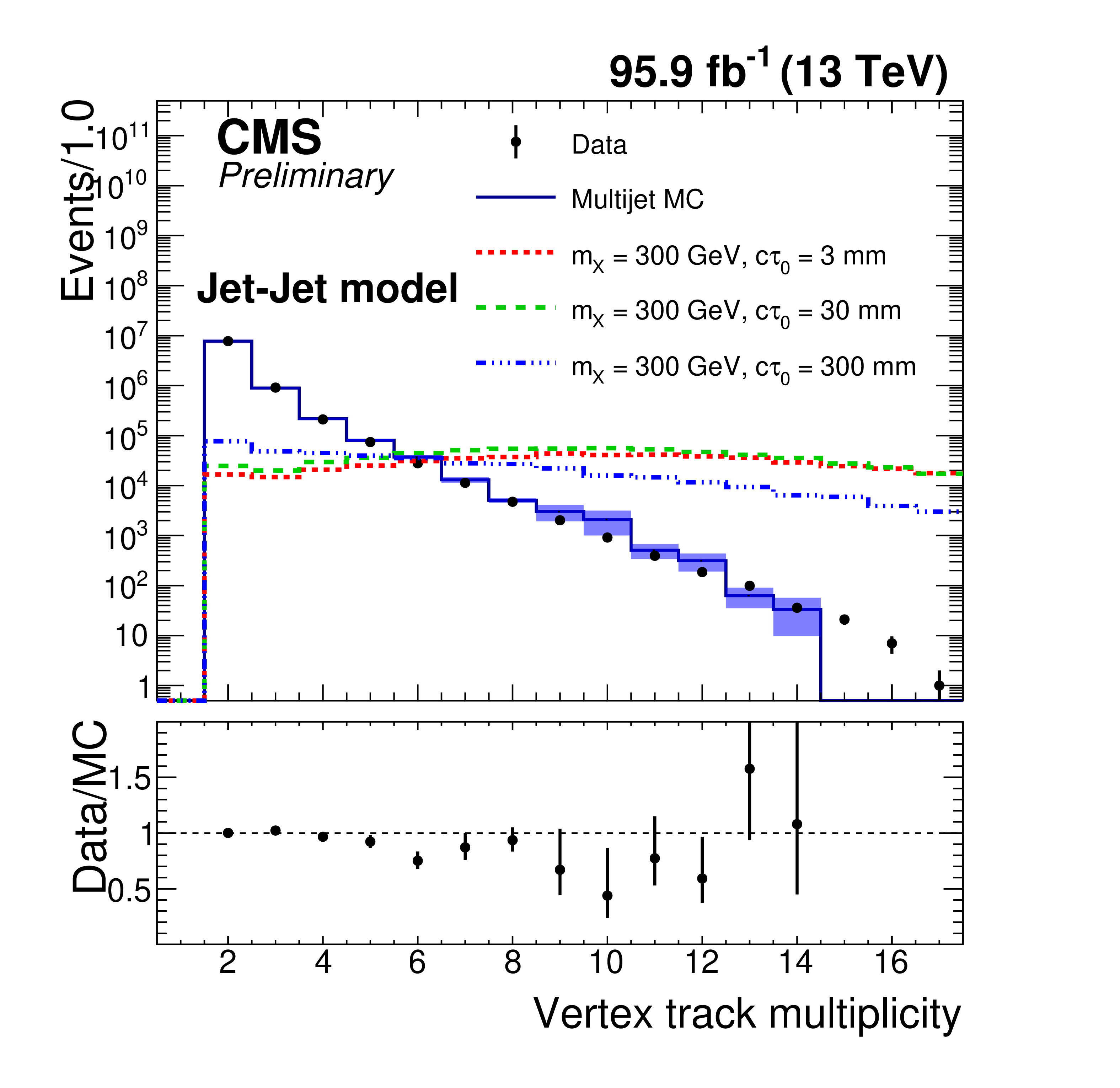
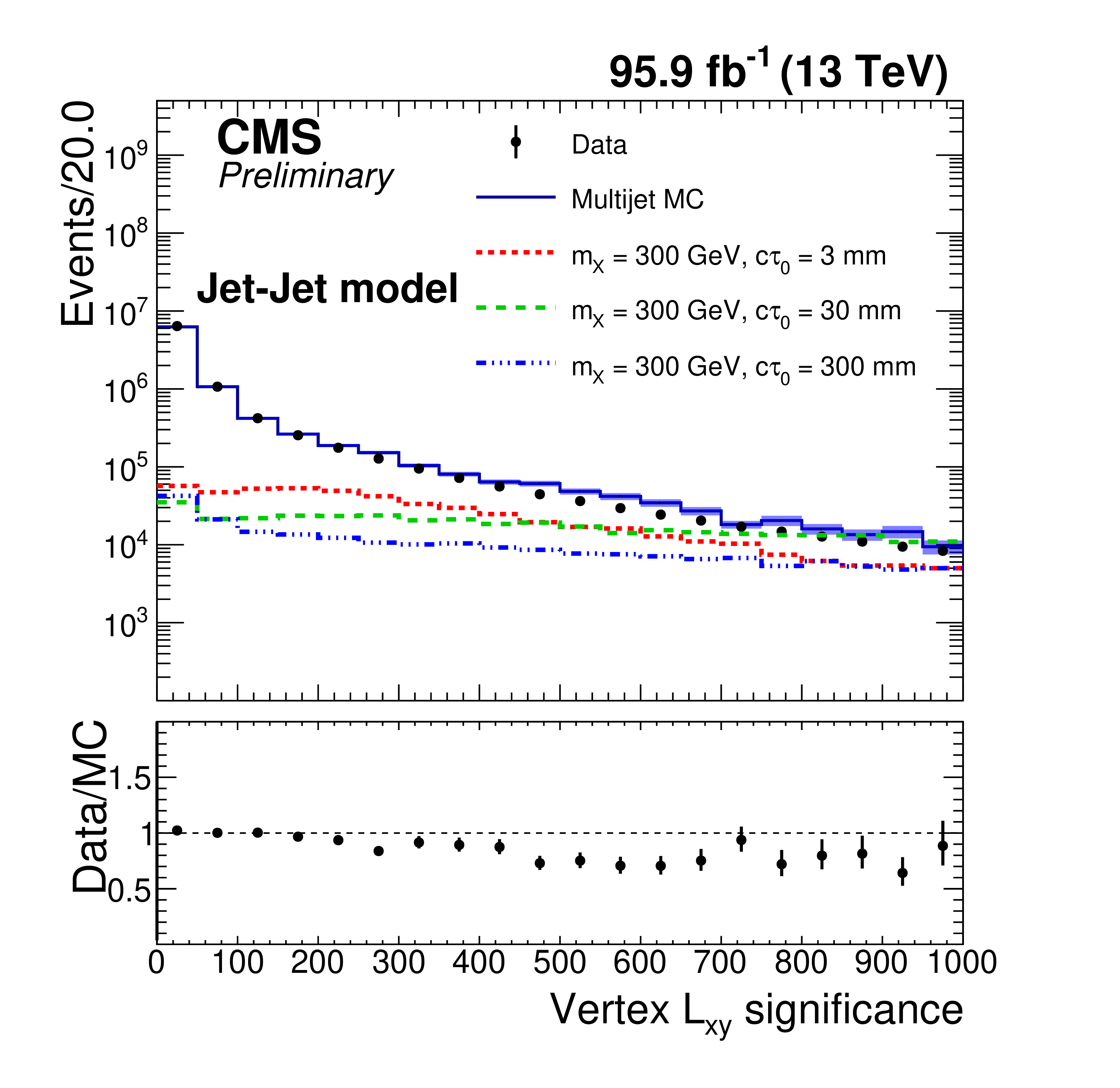
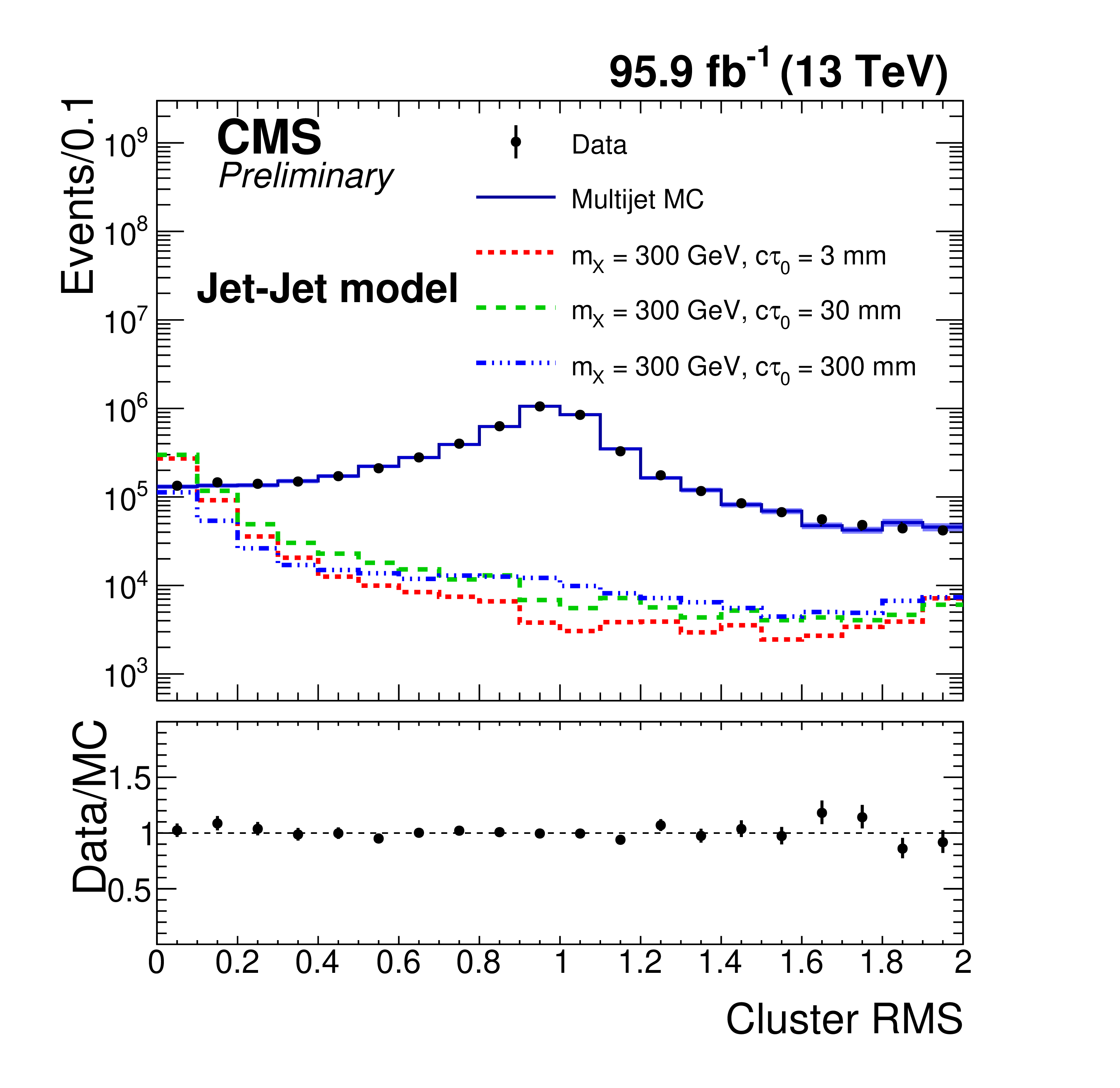
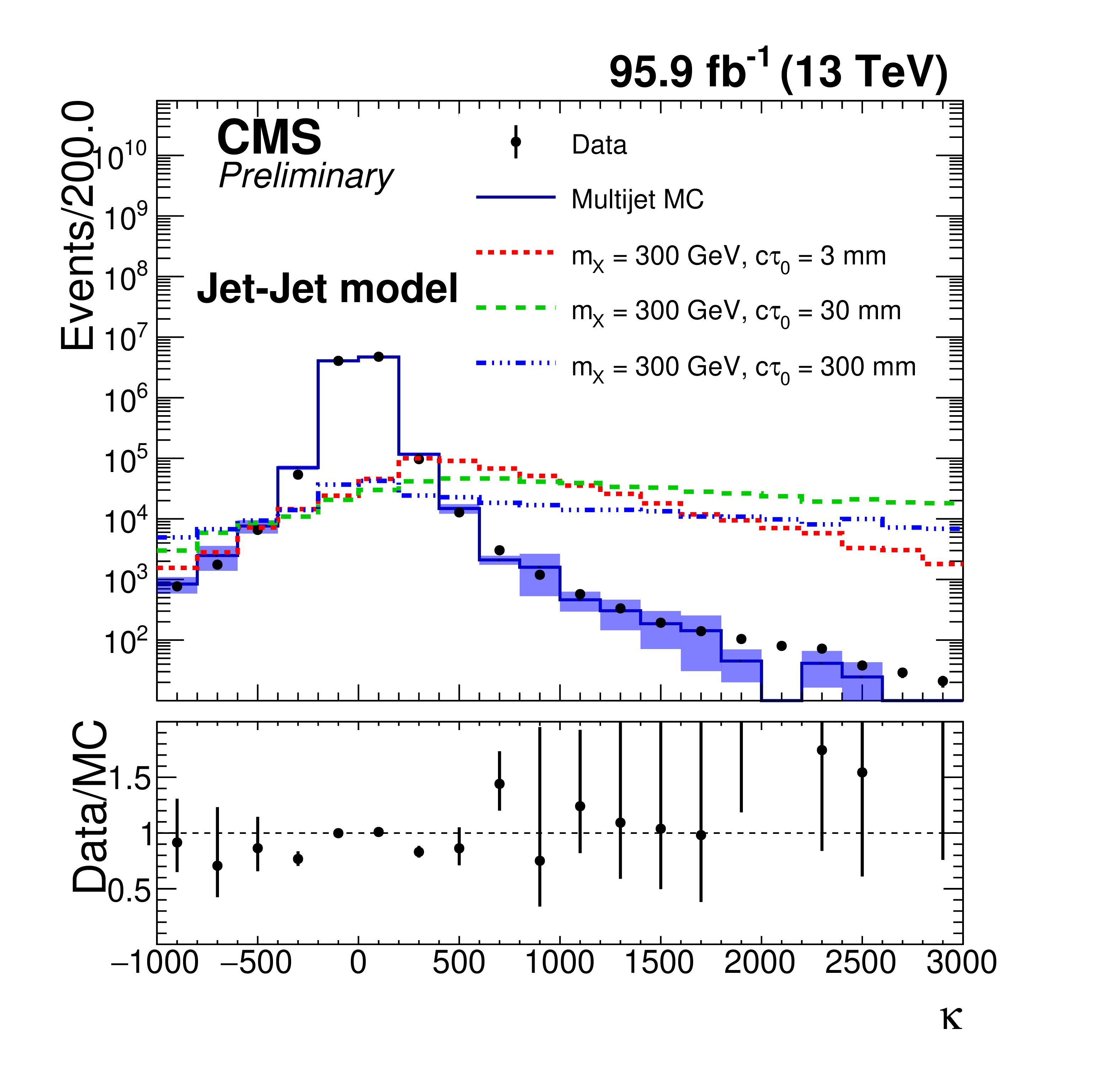
Figure 3:
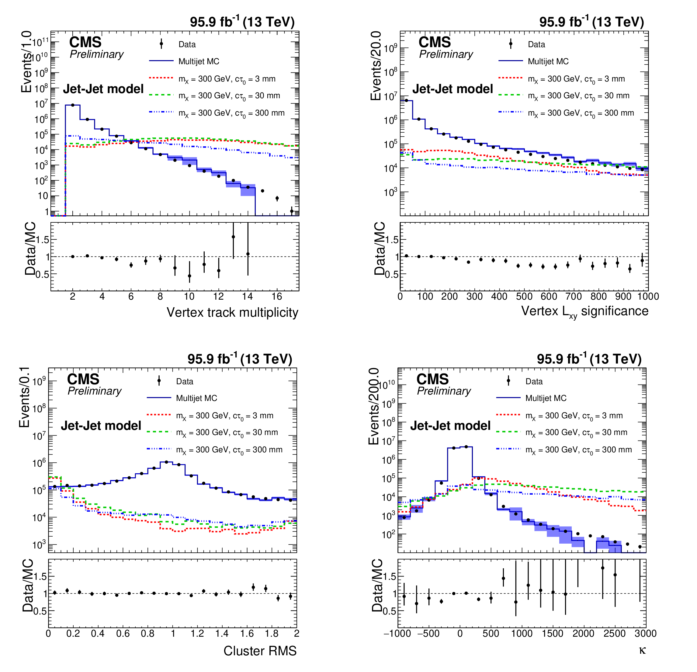
The distributions of the vertex track multiplicity (upper left), vertex $L_{xy}$ significance (upper right), cluster RMS (lower left), and $\kappa $ (lower right), for data, simulated QCD events, and simulated signal events. Data and simulated events are selected with the displaced-jet triggers, with the offline $ {H_{\mathrm {T}}} $, jets $ {p_{\mathrm {T}}} $, and $\eta $ selections applied. The error bands and bars represent the statistical uncertainties. Three benchmark signal distributions are shown (dashed lines) for the jet-jet model with $m_{\mathrm{X}} = $ 300 GeV and varying $c\tau _{0}$. For visualization each signal process is given a cross section, $\sigma $, such that $\sigma \times $ 95.9 fb$^{-1}$ $=$ 1$\times$ 10$^{6}$. |
png pdf |
Figure 3-a:
The distributions of the vertex track multiplicity (upper left), vertex $L_{xy}$ significance (upper right), cluster RMS (lower left), and $\kappa $ (lower right), for data, simulated QCD events, and simulated signal events. Data and simulated events are selected with the displaced-jet triggers, with the offline $ {H_{\mathrm {T}}} $, jets $ {p_{\mathrm {T}}} $, and $\eta $ selections applied. The error bands and bars represent the statistical uncertainties. Three benchmark signal distributions are shown (dashed lines) for the jet-jet model with $m_{\mathrm{X}} = $ 300 GeV and varying $c\tau _{0}$. For visualization each signal process is given a cross section, $\sigma $, such that $\sigma \times $ 95.9 fb$^{-1}$ $=$ 1$\times$ 10$^{6}$. |
png pdf |
Figure 3-b:
The distributions of the vertex track multiplicity (upper left), vertex $L_{xy}$ significance (upper right), cluster RMS (lower left), and $\kappa $ (lower right), for data, simulated QCD events, and simulated signal events. Data and simulated events are selected with the displaced-jet triggers, with the offline $ {H_{\mathrm {T}}} $, jets $ {p_{\mathrm {T}}} $, and $\eta $ selections applied. The error bands and bars represent the statistical uncertainties. Three benchmark signal distributions are shown (dashed lines) for the jet-jet model with $m_{\mathrm{X}} = $ 300 GeV and varying $c\tau _{0}$. For visualization each signal process is given a cross section, $\sigma $, such that $\sigma \times $ 95.9 fb$^{-1}$ $=$ 1$\times$ 10$^{6}$. |
png pdf |
Figure 3-c:
The distributions of the vertex track multiplicity (upper left), vertex $L_{xy}$ significance (upper right), cluster RMS (lower left), and $\kappa $ (lower right), for data, simulated QCD events, and simulated signal events. Data and simulated events are selected with the displaced-jet triggers, with the offline $ {H_{\mathrm {T}}} $, jets $ {p_{\mathrm {T}}} $, and $\eta $ selections applied. The error bands and bars represent the statistical uncertainties. Three benchmark signal distributions are shown (dashed lines) for the jet-jet model with $m_{\mathrm{X}} = $ 300 GeV and varying $c\tau _{0}$. For visualization each signal process is given a cross section, $\sigma $, such that $\sigma \times $ 95.9 fb$^{-1}$ $=$ 1$\times$ 10$^{6}$. |
png pdf |
Figure 3-d:
The distributions of the vertex track multiplicity (upper left), vertex $L_{xy}$ significance (upper right), cluster RMS (lower left), and $\kappa $ (lower right), for data, simulated QCD events, and simulated signal events. Data and simulated events are selected with the displaced-jet triggers, with the offline $ {H_{\mathrm {T}}} $, jets $ {p_{\mathrm {T}}} $, and $\eta $ selections applied. The error bands and bars represent the statistical uncertainties. Three benchmark signal distributions are shown (dashed lines) for the jet-jet model with $m_{\mathrm{X}} = $ 300 GeV and varying $c\tau _{0}$. For visualization each signal process is given a cross section, $\sigma $, such that $\sigma \times $ 95.9 fb$^{-1}$ $=$ 1$\times$ 10$^{6}$. |
png pdf |
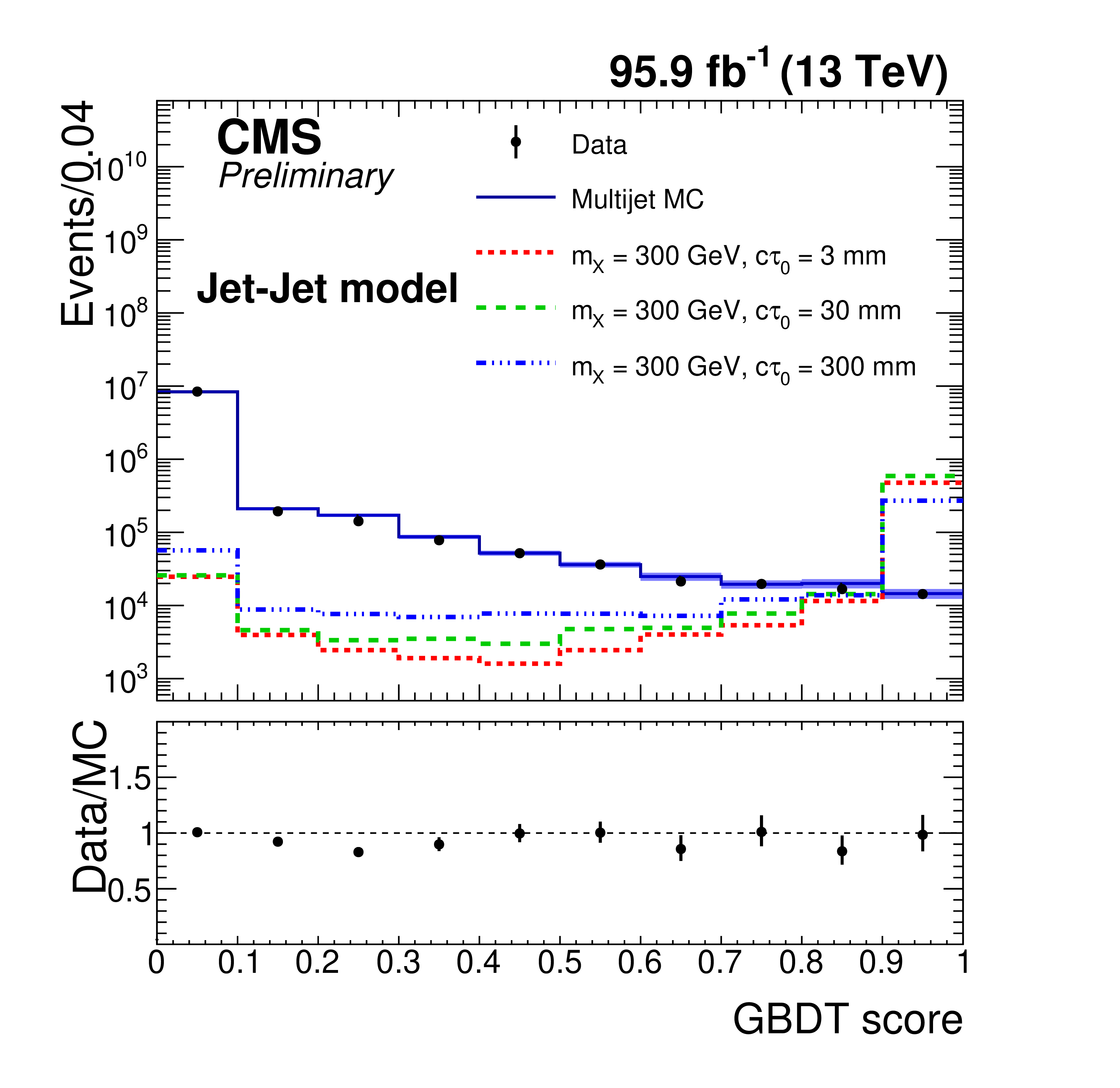
Figure 4:
The distributions of the GBDT output for data, simulated QCD events, and simulated signal events. Data and simulated events are selected with the displaced-jet triggers, with the offline $ {H_{\mathrm {T}}} $, jets $ {p_{\mathrm {T}}} $, and $\eta $ selections applied. The error bands and bars represent the statistical uncertainties. Three benchmark signal distributions are shown (dashed lines) for the jet-jet model with $m_{\mathrm{X}} = $ 300 GeV and varying $c\tau _{0}$. For visualization each signal process is given a cross section, $\sigma $, such that $\sigma \times $ 95.9 fb$^{-1}$ $=$ 1$\times $10$^{6}$. The signal events shown in this plot are not used in the GBDT training. |
png pdf |
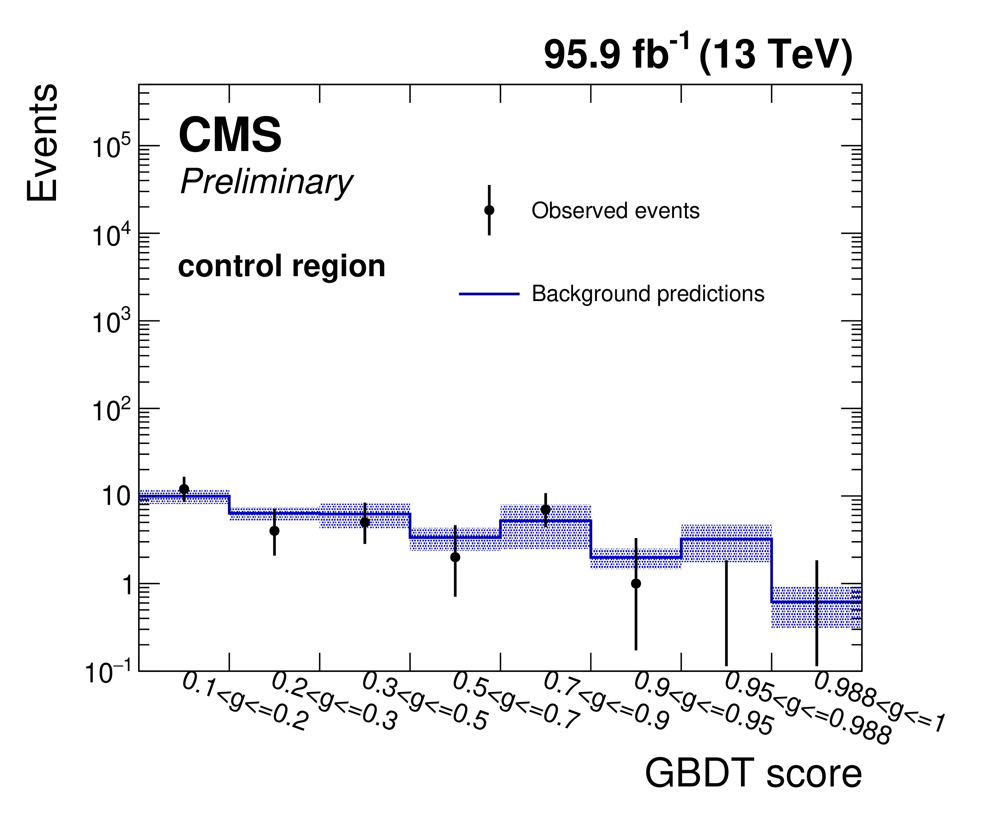
Figure 5:
The predicted background yields and the observed events in the control region, for different bins of the GBDT scores. The error bands for the predictions represent statistical uncertainties and systematic uncertainties added in quadrature. The error bars for the observed events represent statistical uncertainties assuming Poisson statistics. |
png pdf |
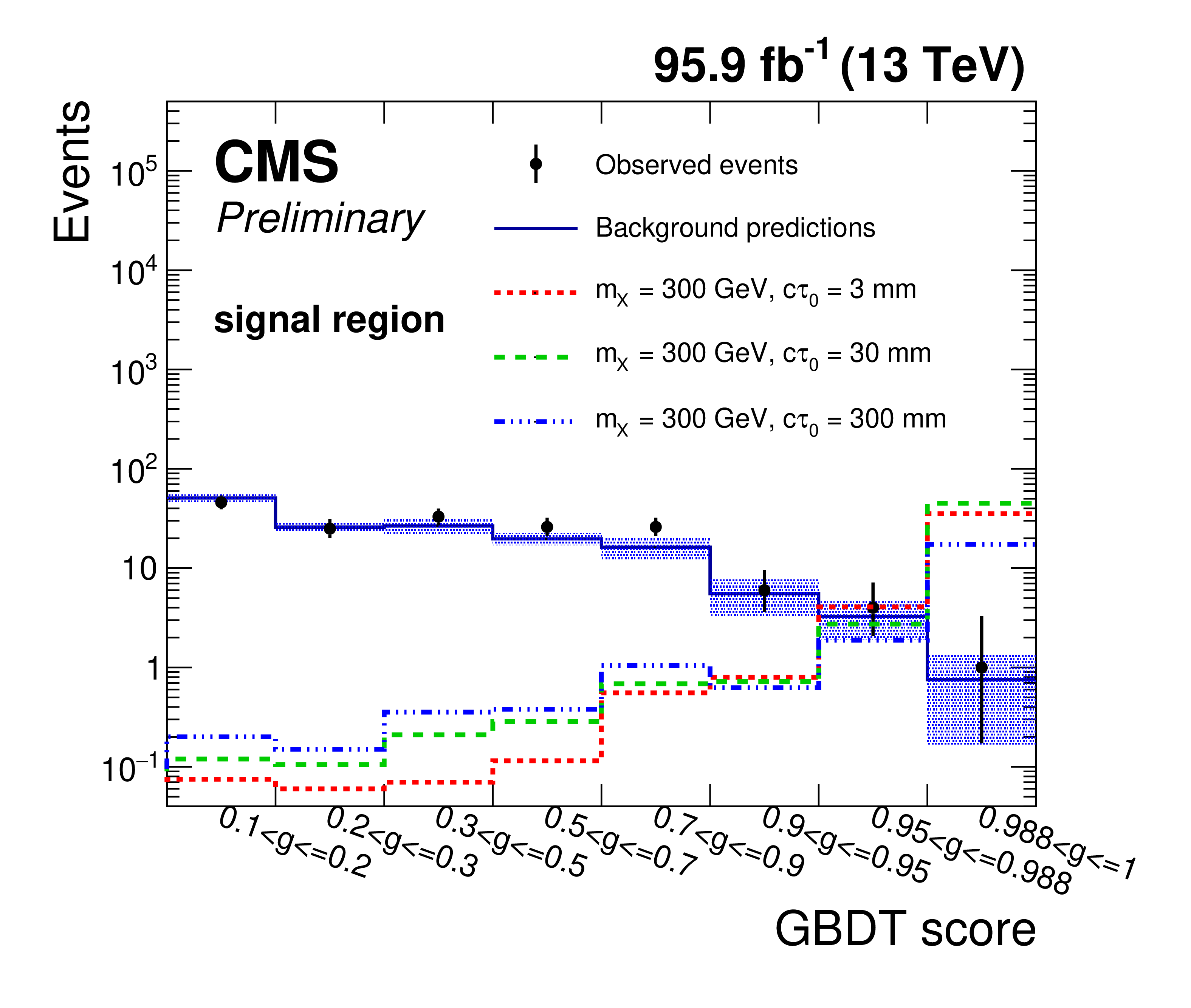
Figure 6:
The predicted background yields and the number of observed events for the data in the signal region, with fewer than three 3D prompt tracks for both jets. The background predictions in different bins are correlated, since the events that are used for background predictions in lower bins are also used in the background predictions in higher bins. For comparison three benchmark signal points are also shown (dashed lines) for the jet-jet model with $m_{\mathrm{X}} = $ 300 GeV and varying lifetimes. For visualization, each signal process is given a cross section, $\sigma $, such that $\sigma \times L= $ 1$\times $10$^{2}$. |
png pdf |
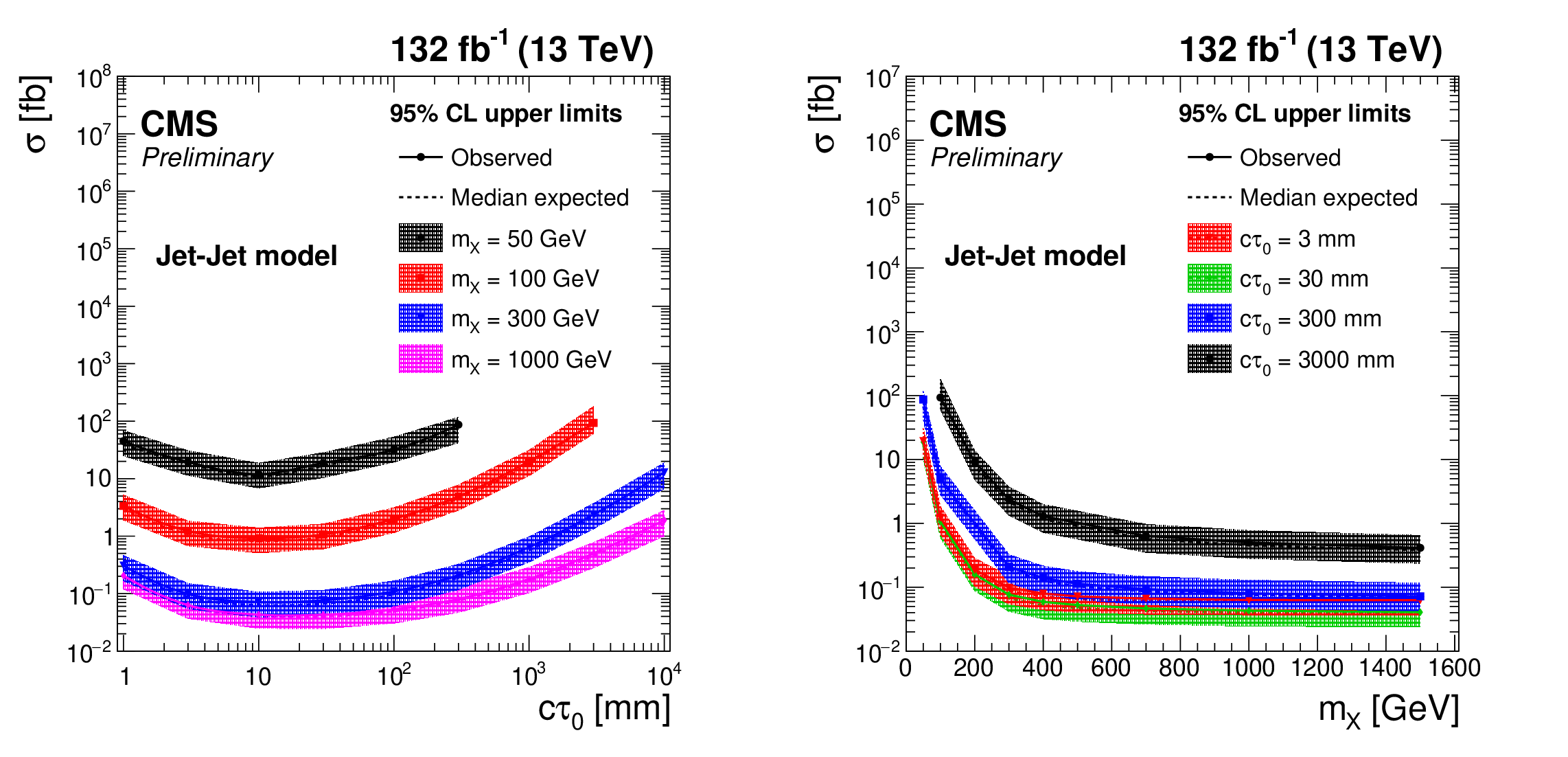
Figure 7:
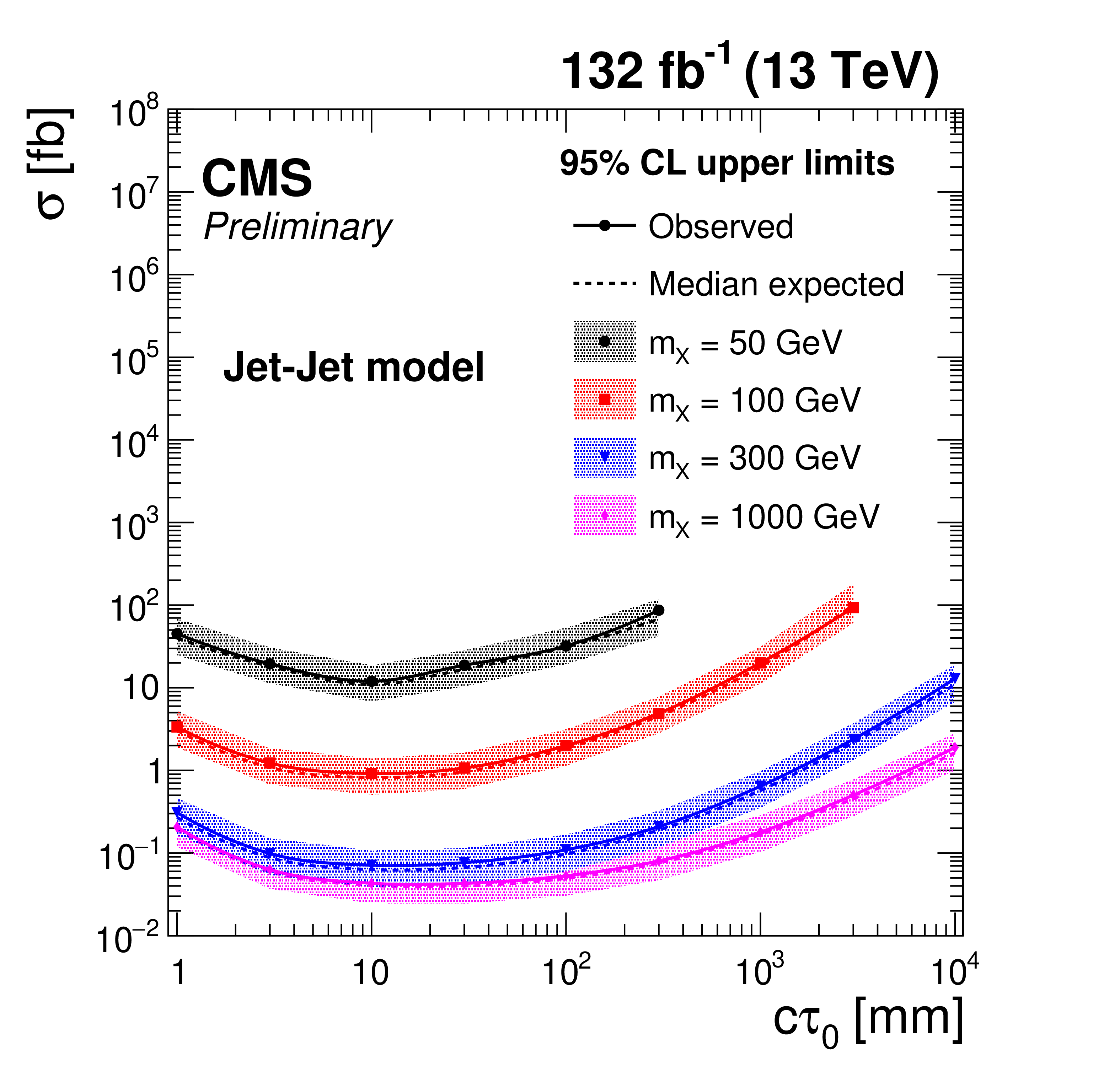
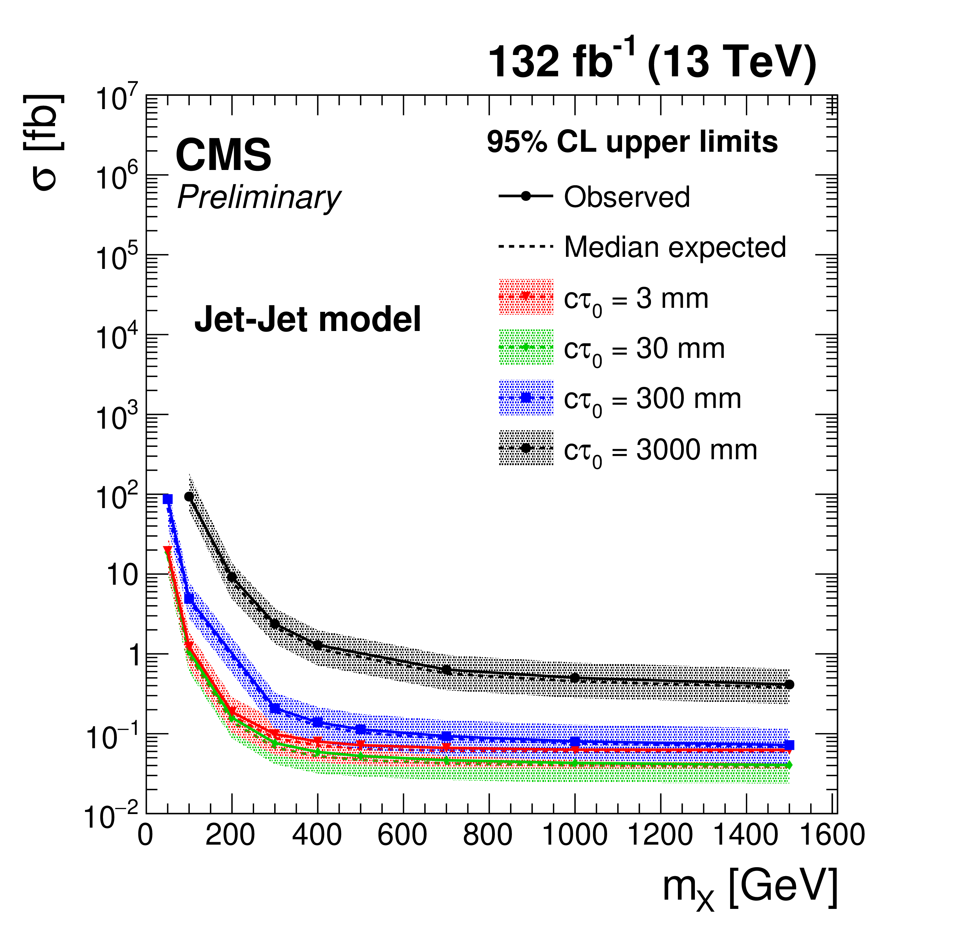
The expected and observed 95% CL upper limits on the pair production cross section of the long-lived particle X, assuming a 100% branching fraction for X to decay to a quark-antiquark pair, shown at different particle X masses and $c\tau _{0}$ for the jet-jet model. The solid (dashed) lines represent the observed (median expected) limits. The shaded bands represent the regions containing 68% of the distributions of the expected limits under the background-only hypothesis. The left plot shows the upper limits as a function of $c\tau _{0}$ for different masses, while the right plot shows the upper limits as a function of the particle mass for different $c\tau _{0}$. |
png pdf |
Figure 7-a:
The expected and observed 95% CL upper limits on the pair production cross section of the long-lived particle X, assuming a 100% branching fraction for X to decay to a quark-antiquark pair, shown at different particle X masses and $c\tau _{0}$ for the jet-jet model. The solid (dashed) lines represent the observed (median expected) limits. The shaded bands represent the regions containing 68% of the distributions of the expected limits under the background-only hypothesis. The left plot shows the upper limits as a function of $c\tau _{0}$ for different masses, while the right plot shows the upper limits as a function of the particle mass for different $c\tau _{0}$. |
png pdf |
Figure 7-b:
The expected and observed 95% CL upper limits on the pair production cross section of the long-lived particle X, assuming a 100% branching fraction for X to decay to a quark-antiquark pair, shown at different particle X masses and $c\tau _{0}$ for the jet-jet model. The solid (dashed) lines represent the observed (median expected) limits. The shaded bands represent the regions containing 68% of the distributions of the expected limits under the background-only hypothesis. The left plot shows the upper limits as a function of $c\tau _{0}$ for different masses, while the right plot shows the upper limits as a function of the particle mass for different $c\tau _{0}$. |
png pdf |
Figure 8:
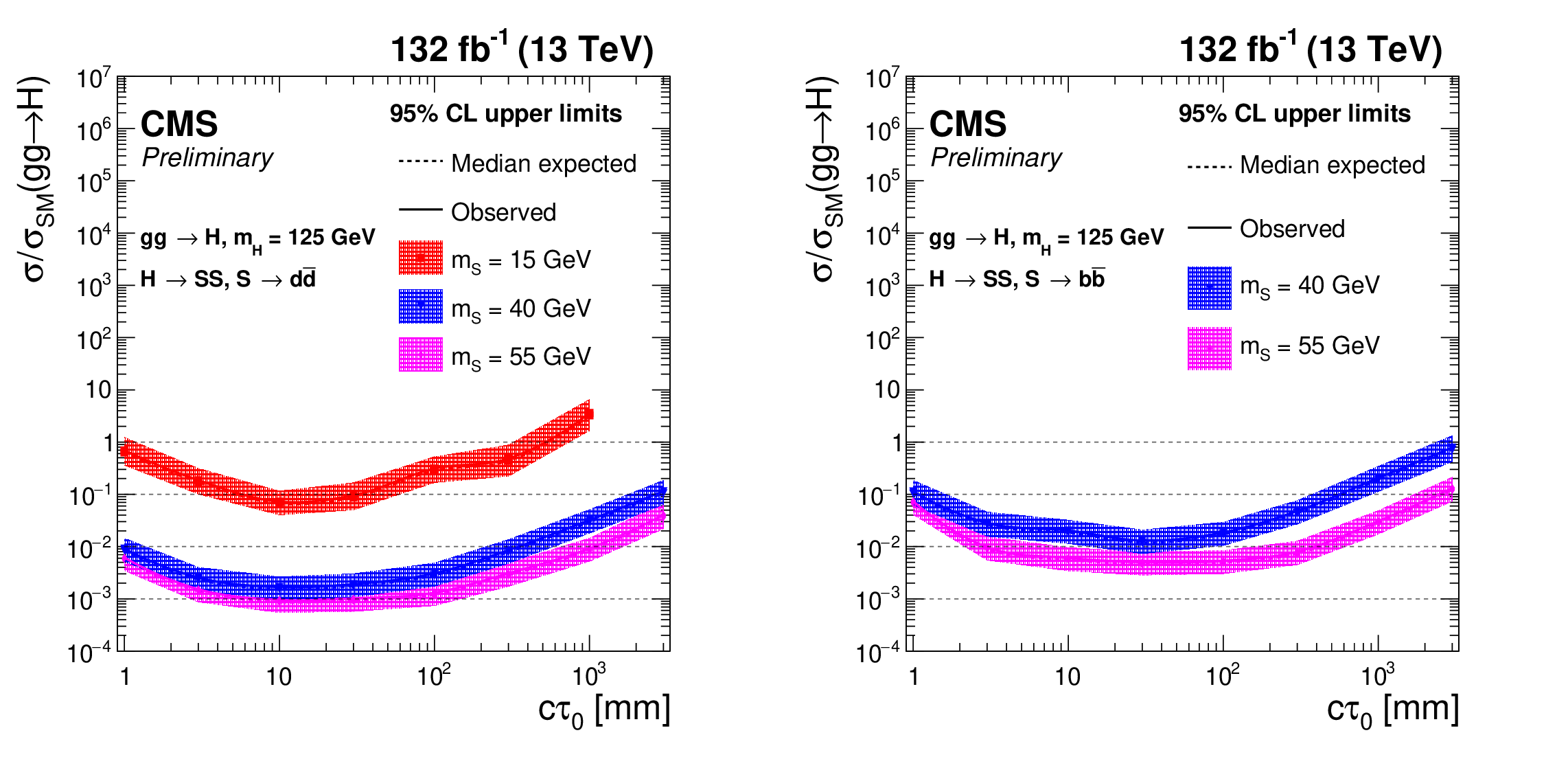
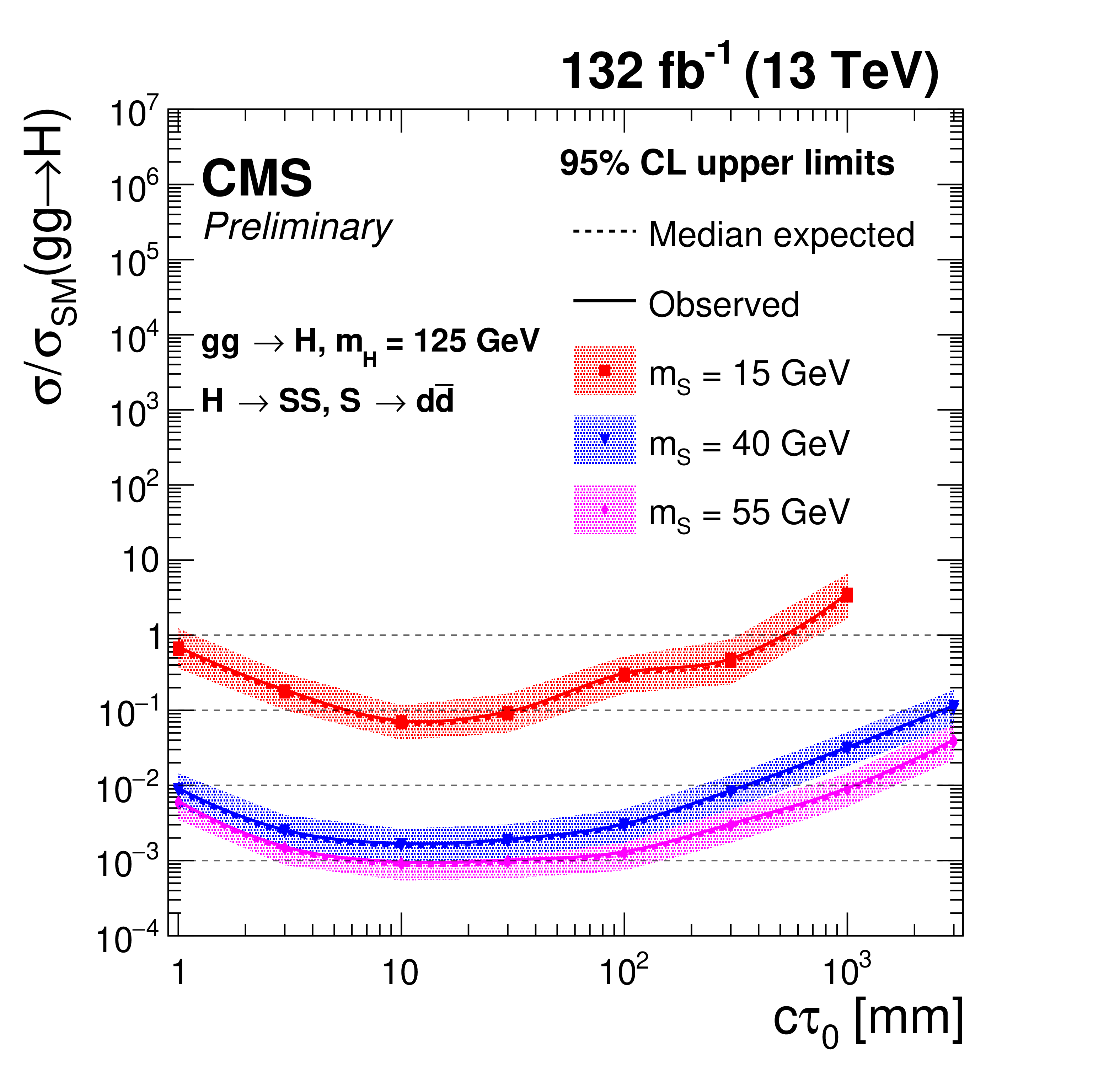
The expected and observed 95% CL upper limits on the branching fraction of the SM Higgs boson to decay to two long-lived scalars, assuming the gluon-gluon fusion SM Higgs production cross section of 49 pb at 13 TeV with $m_{\mathrm{H}} = $ 125 GeV, shown at different masses and $c\tau _{0}$ for the scalar S. The solid (dashed) lines represent the observed (median expected) limits. The shaded bands represent the regions containing 68% of the distributions of the expected limits under the background-only hypothesis. The left plot shows the upper limits when each scalar decays to a down quark-antiquark pair, while the right plot shows the upper limits when each scalar decays to a bottom quark-antiquark pair. |
png pdf |
Figure 8-a:
The expected and observed 95% CL upper limits on the branching fraction of the SM Higgs boson to decay to two long-lived scalars, assuming the gluon-gluon fusion SM Higgs production cross section of 49 pb at 13 TeV with $m_{\mathrm{H}} = $ 125 GeV, shown at different masses and $c\tau _{0}$ for the scalar S. The solid (dashed) lines represent the observed (median expected) limits. The shaded bands represent the regions containing 68% of the distributions of the expected limits under the background-only hypothesis. The left plot shows the upper limits when each scalar decays to a down quark-antiquark pair, while the right plot shows the upper limits when each scalar decays to a bottom quark-antiquark pair. |

png pdf |
Figure 8-b:
The expected and observed 95% CL upper limits on the branching fraction of the SM Higgs boson to decay to two long-lived scalars, assuming the gluon-gluon fusion SM Higgs production cross section of 49 pb at 13 TeV with $m_{\mathrm{H}} = $ 125 GeV, shown at different masses and $c\tau _{0}$ for the scalar S. The solid (dashed) lines represent the observed (median expected) limits. The shaded bands represent the regions containing 68% of the distributions of the expected limits under the background-only hypothesis. The left plot shows the upper limits when each scalar decays to a down quark-antiquark pair, while the right plot shows the upper limits when each scalar decays to a bottom quark-antiquark pair. |
png pdf |
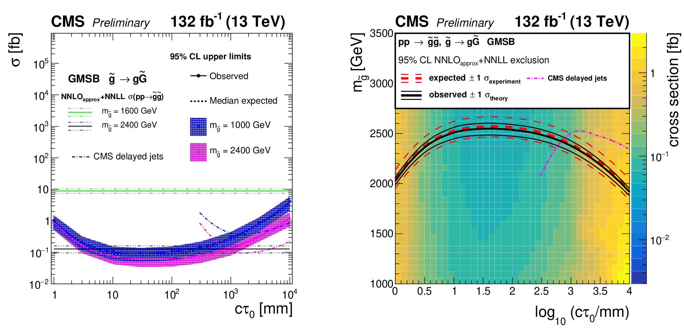
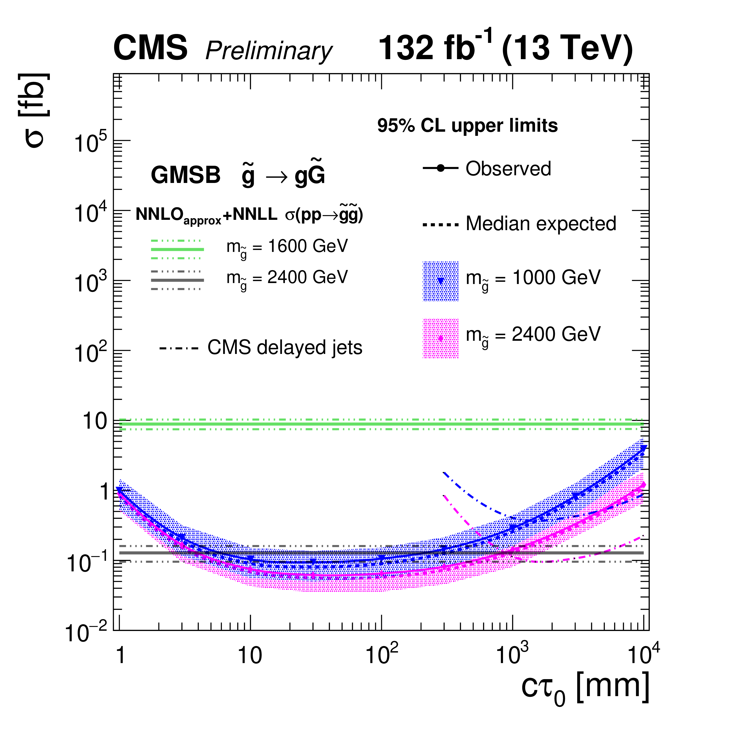
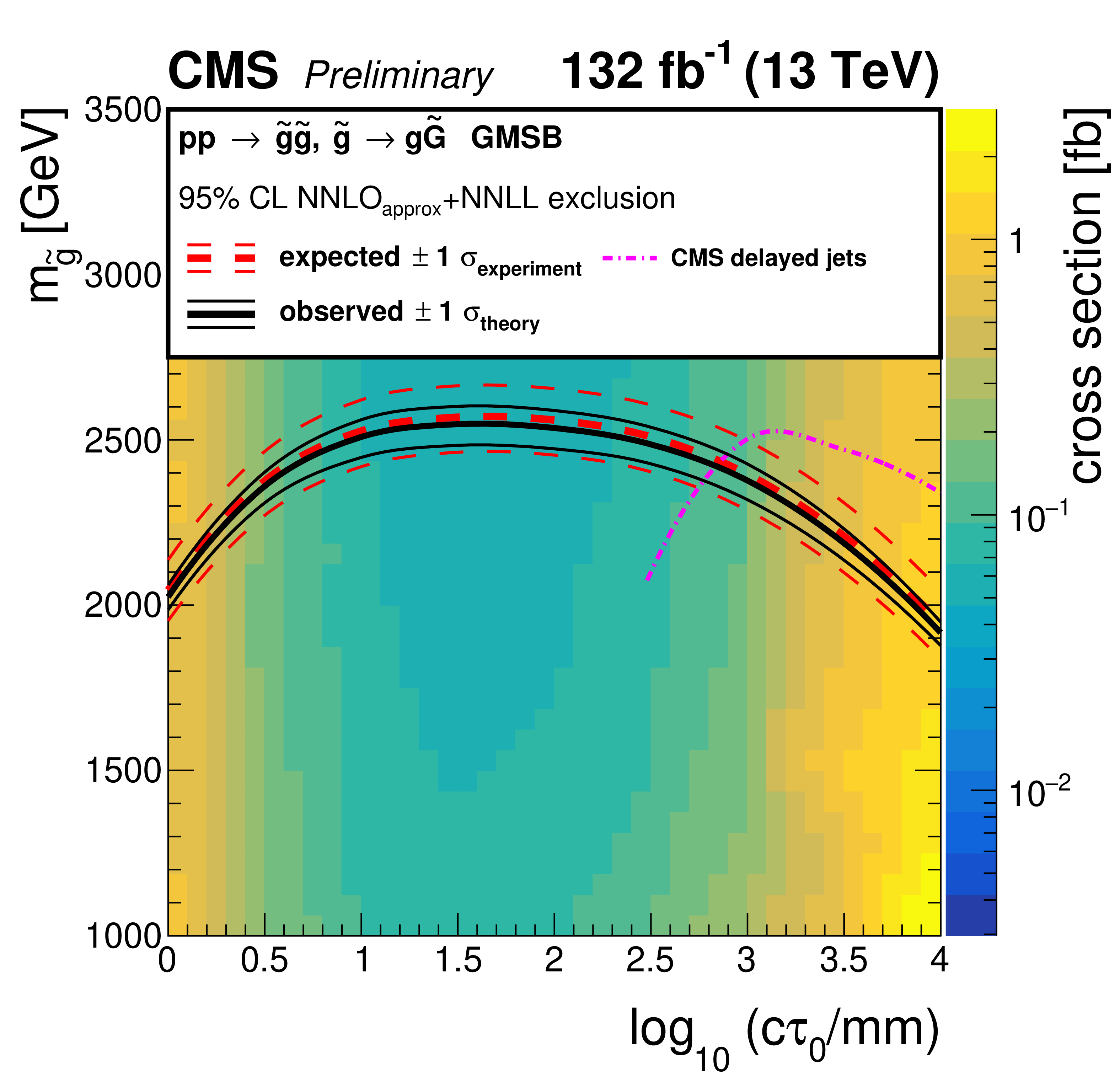
Figure 9:
Left: the expected and observed 95% CL upper limits on the pair production cross section of the long-lived gluinos, assuming a 100% branching fraction for ${\mathrm{\tilde{g}}} \to \mathrm{g} \tilde{\mathrm{G}} $ decays. The horizontal lines indicate the NNLO$_{approx}$+NNLL gluino pair production cross sections for $m_{{\mathrm{\tilde{g}}}} = $ 2400 GeV and $m_{{\mathrm{\tilde{g}}}} = $ 1600 GeV, as well as their variations due to the uncertainties in the choices of renormalization scales, factorization scales, and PDF sets. The solid (dashed) lines represent the observed (median expected) limits, the bands show the regions containing 68% of the distributions of the expected limits under the background-only hypothesis. The observed limits from the CMS search utilizing the timing capabilities of the ECAL system [47] are also shown for comparison. Right: the expected and observed 95% CL limits for the long-lived gluino model in the mass-lifetime plane, assuming a 100% branching fraction for ${\mathrm{\tilde{g}}} \to \mathrm{g} \tilde{\mathrm{G}} $ decays, based on the NNLO$_{approx}$+NNLL calculation of the gluino pair production cross section at $\sqrt {s} = $ 13 TeV. The thick solid black (dashed red) line represents the observed (median expected) limits at 95% CL . The thin red lines indicate the region containing 68% of the distribution of the expected limits under the background-only hypothesis. The thin black lines represent the change in the observed limit due to the variation of the signal cross sections within the theoretical uncertainties. |
png pdf |
Figure 9-a:
Left: the expected and observed 95% CL upper limits on the pair production cross section of the long-lived gluinos, assuming a 100% branching fraction for ${\mathrm{\tilde{g}}} \to \mathrm{g} \tilde{\mathrm{G}} $ decays. The horizontal lines indicate the NNLO$_{approx}$+NNLL gluino pair production cross sections for $m_{{\mathrm{\tilde{g}}}} = $ 2400 GeV and $m_{{\mathrm{\tilde{g}}}} = $ 1600 GeV, as well as their variations due to the uncertainties in the choices of renormalization scales, factorization scales, and PDF sets. The solid (dashed) lines represent the observed (median expected) limits, the bands show the regions containing 68% of the distributions of the expected limits under the background-only hypothesis. The observed limits from the CMS search utilizing the timing capabilities of the ECAL system [47] are also shown for comparison. Right: the expected and observed 95% CL limits for the long-lived gluino model in the mass-lifetime plane, assuming a 100% branching fraction for ${\mathrm{\tilde{g}}} \to \mathrm{g} \tilde{\mathrm{G}} $ decays, based on the NNLO$_{approx}$+NNLL calculation of the gluino pair production cross section at $\sqrt {s} = $ 13 TeV. The thick solid black (dashed red) line represents the observed (median expected) limits at 95% CL . The thin red lines indicate the region containing 68% of the distribution of the expected limits under the background-only hypothesis. The thin black lines represent the change in the observed limit due to the variation of the signal cross sections within the theoretical uncertainties. |
png pdf |
Figure 9-b:
Left: the expected and observed 95% CL upper limits on the pair production cross section of the long-lived gluinos, assuming a 100% branching fraction for ${\mathrm{\tilde{g}}} \to \mathrm{g} \tilde{\mathrm{G}} $ decays. The horizontal lines indicate the NNLO$_{approx}$+NNLL gluino pair production cross sections for $m_{{\mathrm{\tilde{g}}}} = $ 2400 GeV and $m_{{\mathrm{\tilde{g}}}} = $ 1600 GeV, as well as their variations due to the uncertainties in the choices of renormalization scales, factorization scales, and PDF sets. The solid (dashed) lines represent the observed (median expected) limits, the bands show the regions containing 68% of the distributions of the expected limits under the background-only hypothesis. The observed limits from the CMS search utilizing the timing capabilities of the ECAL system [47] are also shown for comparison. Right: the expected and observed 95% CL limits for the long-lived gluino model in the mass-lifetime plane, assuming a 100% branching fraction for ${\mathrm{\tilde{g}}} \to \mathrm{g} \tilde{\mathrm{G}} $ decays, based on the NNLO$_{approx}$+NNLL calculation of the gluino pair production cross section at $\sqrt {s} = $ 13 TeV. The thick solid black (dashed red) line represents the observed (median expected) limits at 95% CL . The thin red lines indicate the region containing 68% of the distribution of the expected limits under the background-only hypothesis. The thin black lines represent the change in the observed limit due to the variation of the signal cross sections within the theoretical uncertainties. |
png pdf |
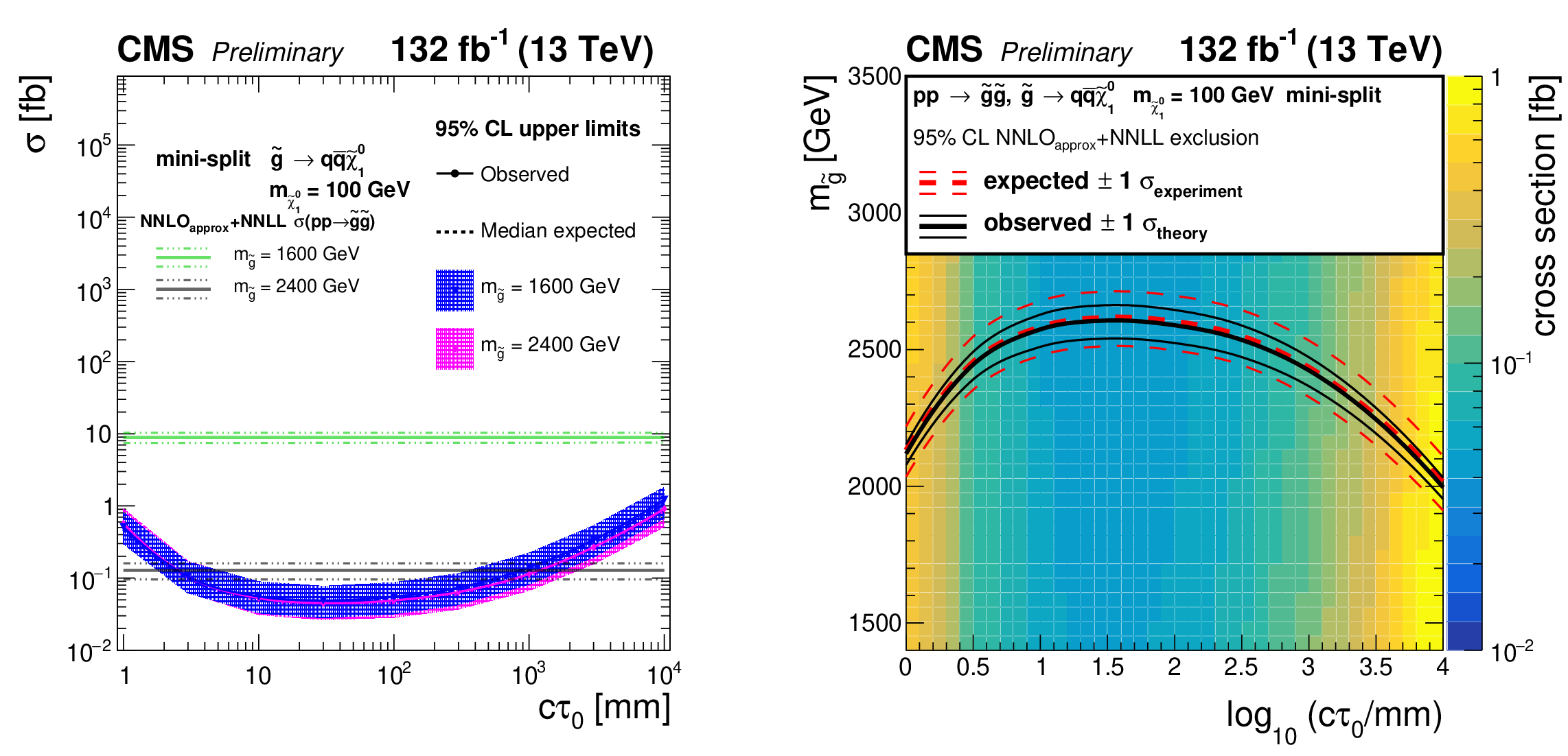
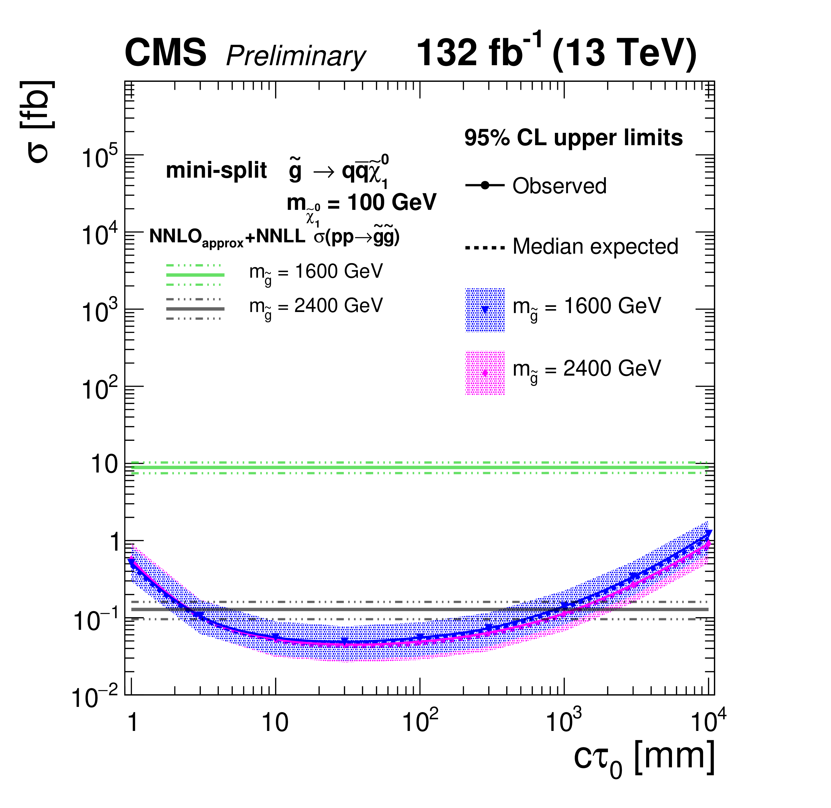
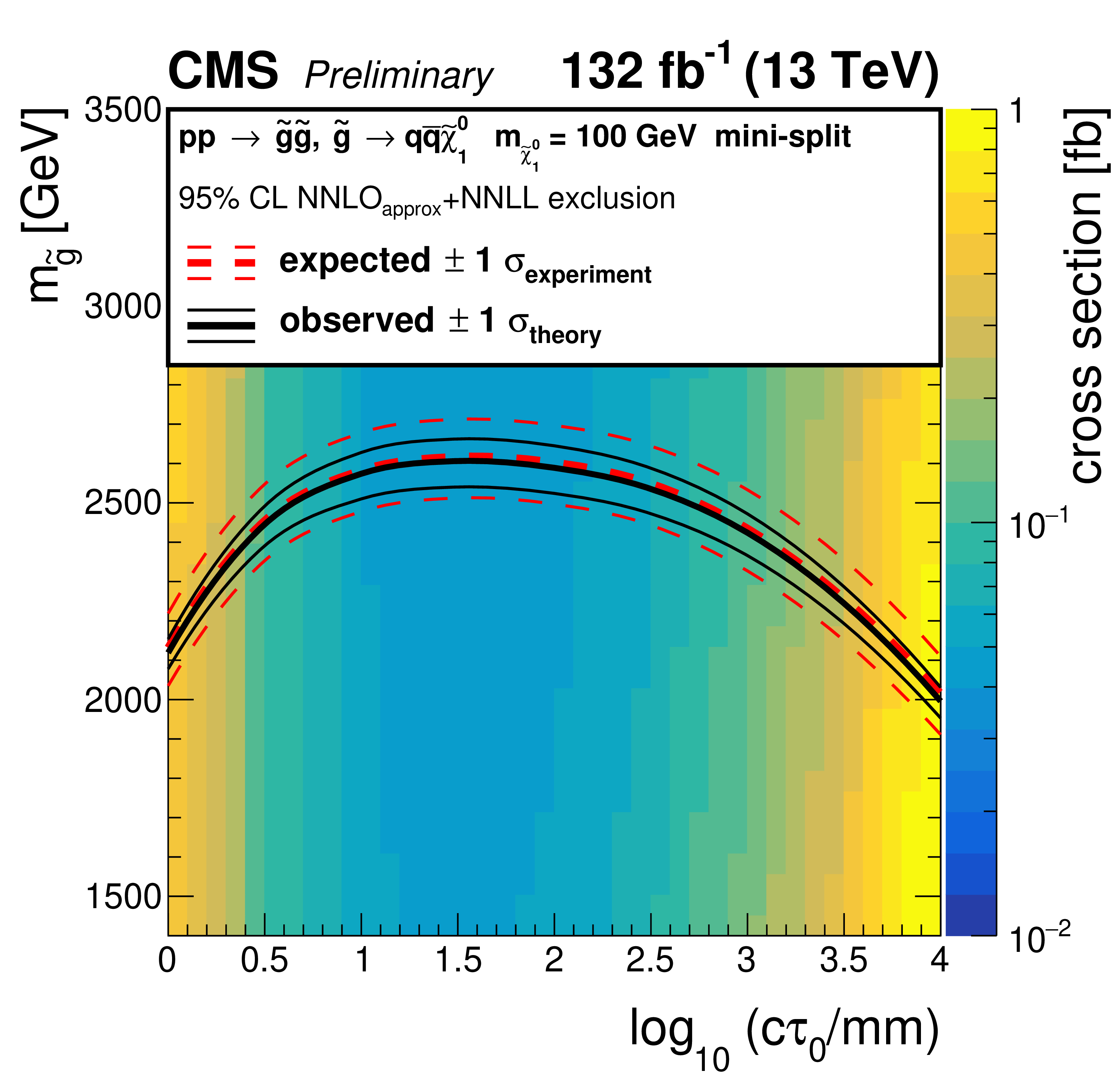
Figure 10:
Left: the expected and observed 95% CL upper limits on the pair production cross section of the long-lived gluinos, assuming a 100% branching fraction for ${\mathrm{\tilde{g}}} \to \mathrm{q} \mathrm{\bar{q}} \tilde{\chi}^{0}_{1}$ decays. The horizontal lines indicate the NNLO$_{approx}$+NNLL gluino pair production cross sections for $m_{{\mathrm{\tilde{g}}}} = $ 2400 GeV and $m_{{\mathrm{\tilde{g}}}} = $ 1600 GeV, as well as their variations due to the uncertainties in the choices of renormalization scales, factorization scales, and PDF sets. The solid (dashed) lines represent the observed (median expected) limits, the bands show the regions containing 68% of the distributions of the expected limits under the background-only hypothesis. Right: the expected and observed 95% CL limits for the long-lived gluino model in the mass-lifetime plane, assuming a 100% branching fraction for ${\mathrm{\tilde{g}}} \to \mathrm{q} \mathrm{\bar{q}} \tilde{\chi}^{0}_{1}$ decays, based on the NNLO$_{approx}$+NNLL calculation of the gluino pair production cross section at $\sqrt {s} = $ 13 TeV. The thick solid black (dashed red) line represents the observed (median expected) limits at 95% CL . The thin red lines indicate the region containing 68% of the distribution of the expected limits under the background-only hypothesis. The thin black lines represent the change in the observed limit due to the variation of the signal cross sections within the theoretical uncertainties. |
png pdf |
Figure 10-a:
Left: the expected and observed 95% CL upper limits on the pair production cross section of the long-lived gluinos, assuming a 100% branching fraction for ${\mathrm{\tilde{g}}} \to \mathrm{q} \mathrm{\bar{q}} \tilde{\chi}^{0}_{1}$ decays. The horizontal lines indicate the NNLO$_{approx}$+NNLL gluino pair production cross sections for $m_{{\mathrm{\tilde{g}}}} = $ 2400 GeV and $m_{{\mathrm{\tilde{g}}}} = $ 1600 GeV, as well as their variations due to the uncertainties in the choices of renormalization scales, factorization scales, and PDF sets. The solid (dashed) lines represent the observed (median expected) limits, the bands show the regions containing 68% of the distributions of the expected limits under the background-only hypothesis. Right: the expected and observed 95% CL limits for the long-lived gluino model in the mass-lifetime plane, assuming a 100% branching fraction for ${\mathrm{\tilde{g}}} \to \mathrm{q} \mathrm{\bar{q}} \tilde{\chi}^{0}_{1}$ decays, based on the NNLO$_{approx}$+NNLL calculation of the gluino pair production cross section at $\sqrt {s} = $ 13 TeV. The thick solid black (dashed red) line represents the observed (median expected) limits at 95% CL . The thin red lines indicate the region containing 68% of the distribution of the expected limits under the background-only hypothesis. The thin black lines represent the change in the observed limit due to the variation of the signal cross sections within the theoretical uncertainties. |
png pdf |
Figure 10-b:
Left: the expected and observed 95% CL upper limits on the pair production cross section of the long-lived gluinos, assuming a 100% branching fraction for ${\mathrm{\tilde{g}}} \to \mathrm{q} \mathrm{\bar{q}} \tilde{\chi}^{0}_{1}$ decays. The horizontal lines indicate the NNLO$_{approx}$+NNLL gluino pair production cross sections for $m_{{\mathrm{\tilde{g}}}} = $ 2400 GeV and $m_{{\mathrm{\tilde{g}}}} = $ 1600 GeV, as well as their variations due to the uncertainties in the choices of renormalization scales, factorization scales, and PDF sets. The solid (dashed) lines represent the observed (median expected) limits, the bands show the regions containing 68% of the distributions of the expected limits under the background-only hypothesis. Right: the expected and observed 95% CL limits for the long-lived gluino model in the mass-lifetime plane, assuming a 100% branching fraction for ${\mathrm{\tilde{g}}} \to \mathrm{q} \mathrm{\bar{q}} \tilde{\chi}^{0}_{1}$ decays, based on the NNLO$_{approx}$+NNLL calculation of the gluino pair production cross section at $\sqrt {s} = $ 13 TeV. The thick solid black (dashed red) line represents the observed (median expected) limits at 95% CL . The thin red lines indicate the region containing 68% of the distribution of the expected limits under the background-only hypothesis. The thin black lines represent the change in the observed limit due to the variation of the signal cross sections within the theoretical uncertainties. |
png pdf |
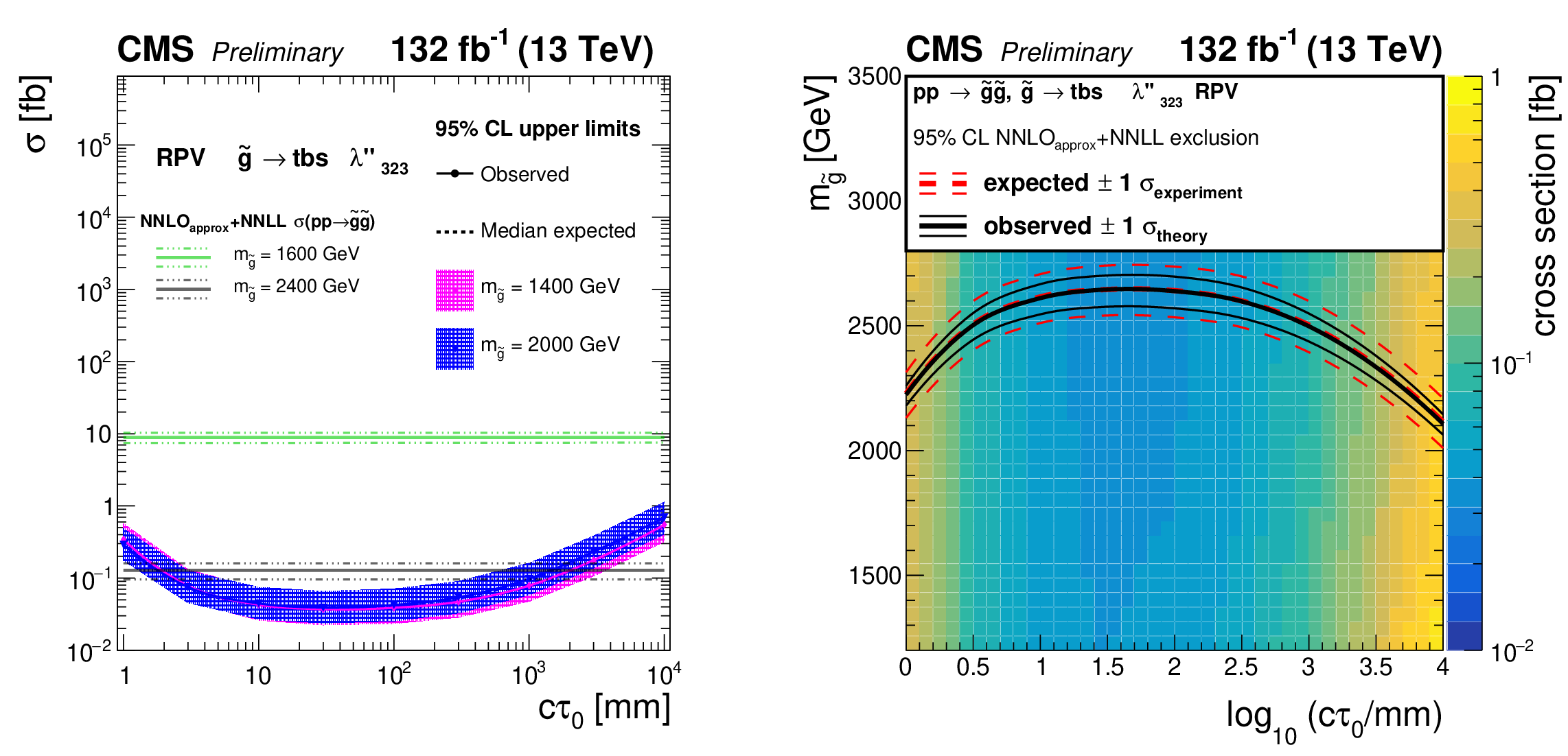
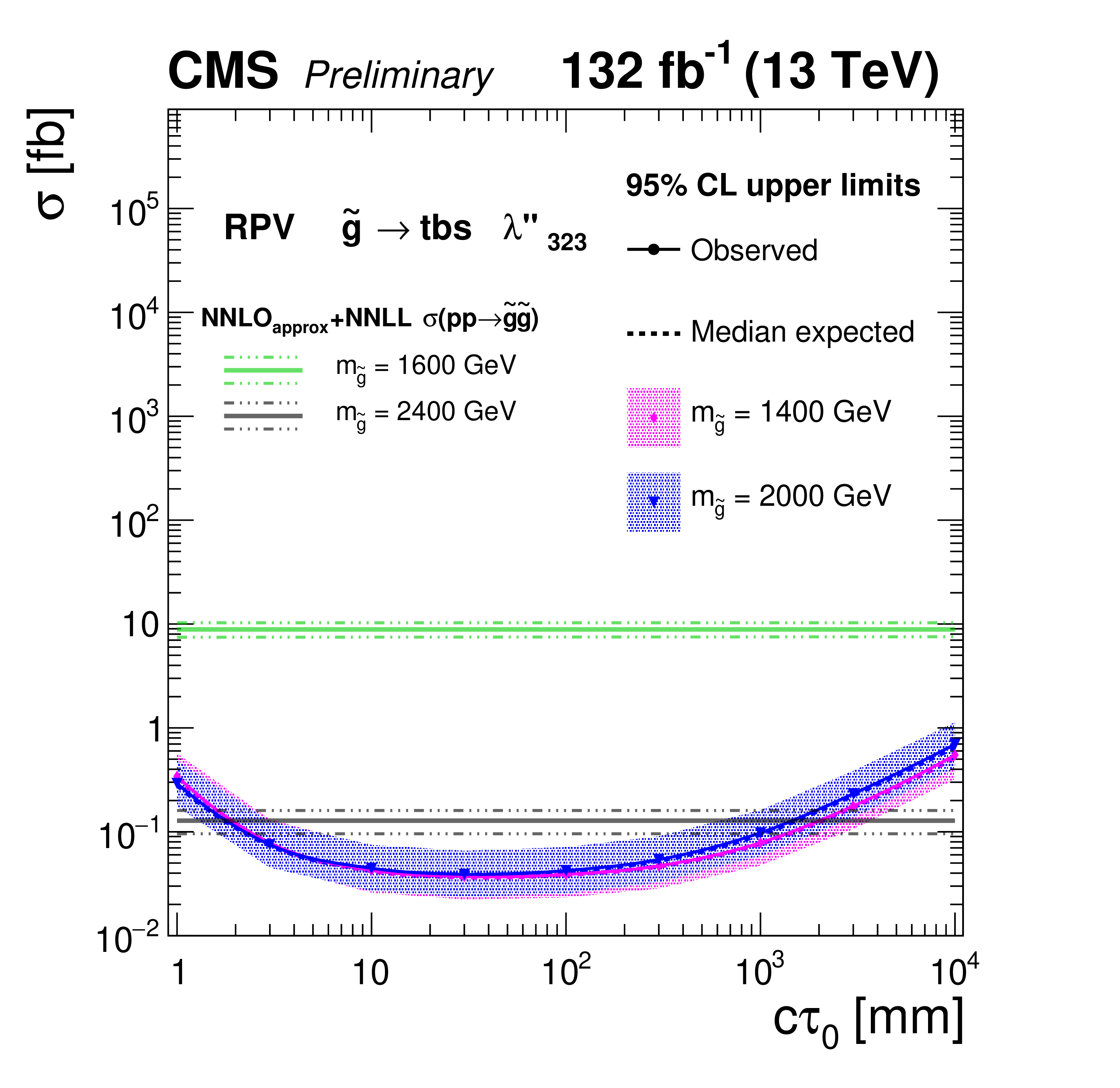
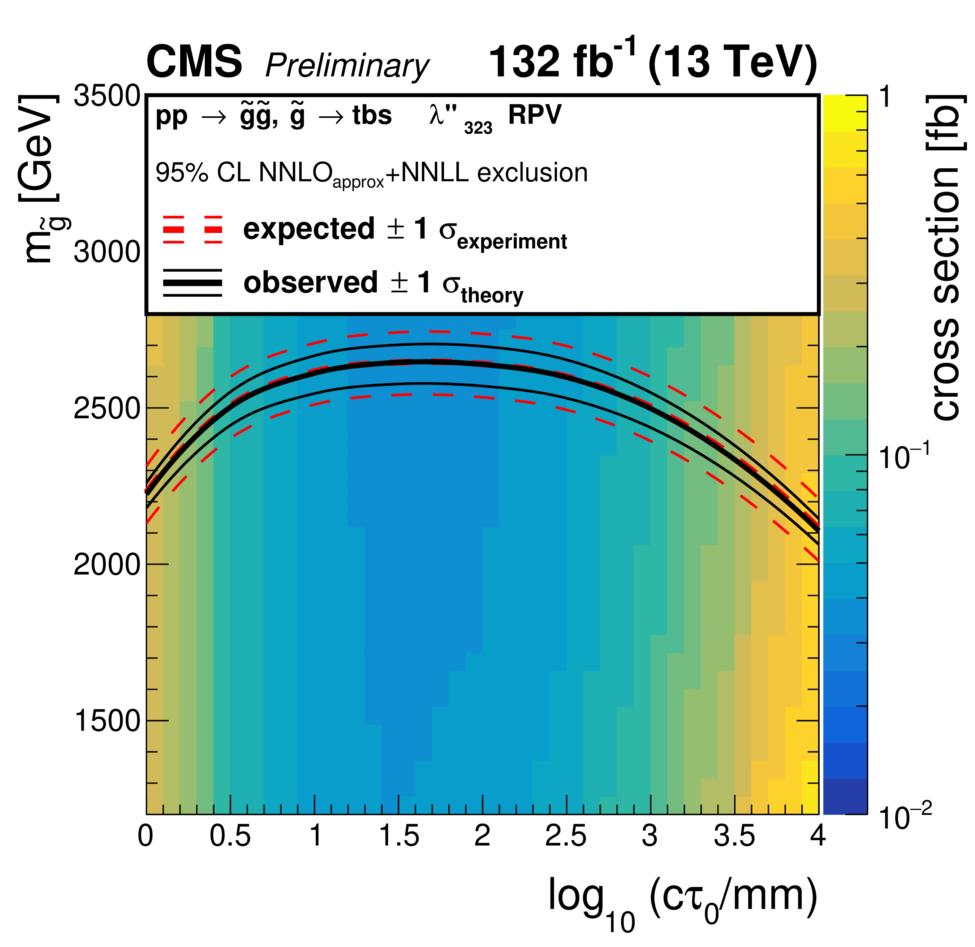
Figure 11:
Left: the expected and observed 95% CL upper limits on the pair production cross section of the long-lived gluinos, assuming a 100% branching fraction for ${\mathrm{\tilde{g}}} \to \mathrm{t} \mathrm{b} \mathrm{s} $ decays. The horizontal lines indicate the NNLO$_{approx}$+NNLL gluino pair production cross sections for $m_{{\mathrm{\tilde{g}}}} = $ 2400 GeV and $m_{{\mathrm{\tilde{g}}}} = $ 1600 GeV, as well as their variations due to the uncertainties in the choices of renormalization scales, factorization scales, and PDF sets. The solid (dashed) lines represent the observed (median expected) limits, the bands show the regions containing 68% of the distributions of the expected limits under the background-only hypothesis. Right: the expected and observed 95% CL limits for the long-lived gluino model in the mass-lifetime plane, assuming a 100% branching fraction for ${\mathrm{\tilde{g}}} \to \mathrm{t} \mathrm{b} \mathrm{s} $ decays, based on the NNLO$_{approx}$+NNLL calculation of the gluino pair production cross section at $\sqrt {s} = $ 13 TeV. The thick solid black (dashed red) line represents the observed (median expected) limits at 95% CL . The thin red lines indicate the region containing 68% of the distribution of the expected limits under the background-only hypothesis. The thin black lines represent the change in the observed limit due to the variation of the signal cross sections within the theoretical uncertainties. |
png pdf |
Figure 11-a:
Left: the expected and observed 95% CL upper limits on the pair production cross section of the long-lived gluinos, assuming a 100% branching fraction for ${\mathrm{\tilde{g}}} \to \mathrm{t} \mathrm{b} \mathrm{s} $ decays. The horizontal lines indicate the NNLO$_{approx}$+NNLL gluino pair production cross sections for $m_{{\mathrm{\tilde{g}}}} = $ 2400 GeV and $m_{{\mathrm{\tilde{g}}}} = $ 1600 GeV, as well as their variations due to the uncertainties in the choices of renormalization scales, factorization scales, and PDF sets. The solid (dashed) lines represent the observed (median expected) limits, the bands show the regions containing 68% of the distributions of the expected limits under the background-only hypothesis. Right: the expected and observed 95% CL limits for the long-lived gluino model in the mass-lifetime plane, assuming a 100% branching fraction for ${\mathrm{\tilde{g}}} \to \mathrm{t} \mathrm{b} \mathrm{s} $ decays, based on the NNLO$_{approx}$+NNLL calculation of the gluino pair production cross section at $\sqrt {s} = $ 13 TeV. The thick solid black (dashed red) line represents the observed (median expected) limits at 95% CL . The thin red lines indicate the region containing 68% of the distribution of the expected limits under the background-only hypothesis. The thin black lines represent the change in the observed limit due to the variation of the signal cross sections within the theoretical uncertainties. |
png pdf |
Figure 11-b:
Left: the expected and observed 95% CL upper limits on the pair production cross section of the long-lived gluinos, assuming a 100% branching fraction for ${\mathrm{\tilde{g}}} \to \mathrm{t} \mathrm{b} \mathrm{s} $ decays. The horizontal lines indicate the NNLO$_{approx}$+NNLL gluino pair production cross sections for $m_{{\mathrm{\tilde{g}}}} = $ 2400 GeV and $m_{{\mathrm{\tilde{g}}}} = $ 1600 GeV, as well as their variations due to the uncertainties in the choices of renormalization scales, factorization scales, and PDF sets. The solid (dashed) lines represent the observed (median expected) limits, the bands show the regions containing 68% of the distributions of the expected limits under the background-only hypothesis. Right: the expected and observed 95% CL limits for the long-lived gluino model in the mass-lifetime plane, assuming a 100% branching fraction for ${\mathrm{\tilde{g}}} \to \mathrm{t} \mathrm{b} \mathrm{s} $ decays, based on the NNLO$_{approx}$+NNLL calculation of the gluino pair production cross section at $\sqrt {s} = $ 13 TeV. The thick solid black (dashed red) line represents the observed (median expected) limits at 95% CL . The thin red lines indicate the region containing 68% of the distribution of the expected limits under the background-only hypothesis. The thin black lines represent the change in the observed limit due to the variation of the signal cross sections within the theoretical uncertainties. |
png pdf |
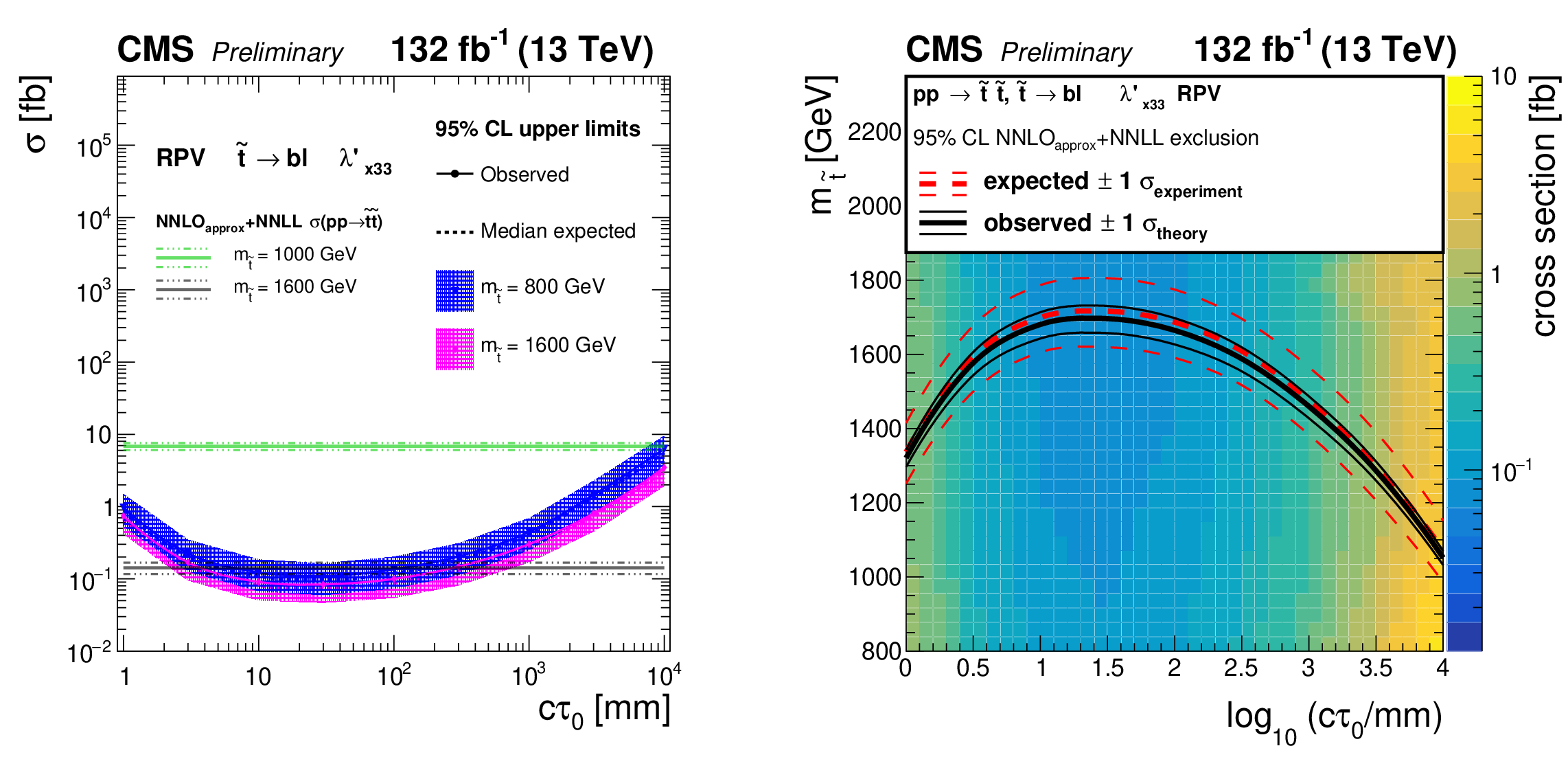
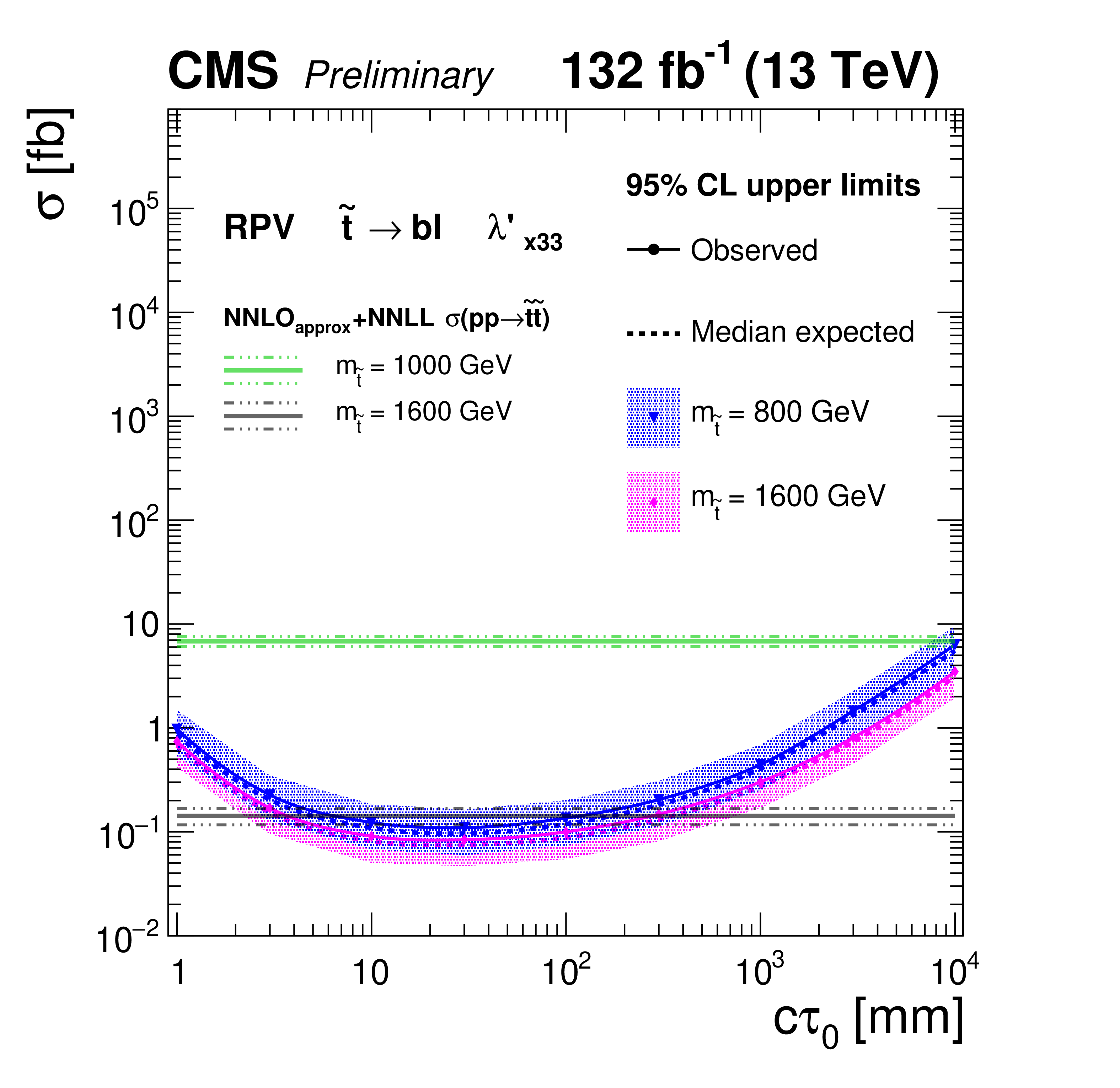
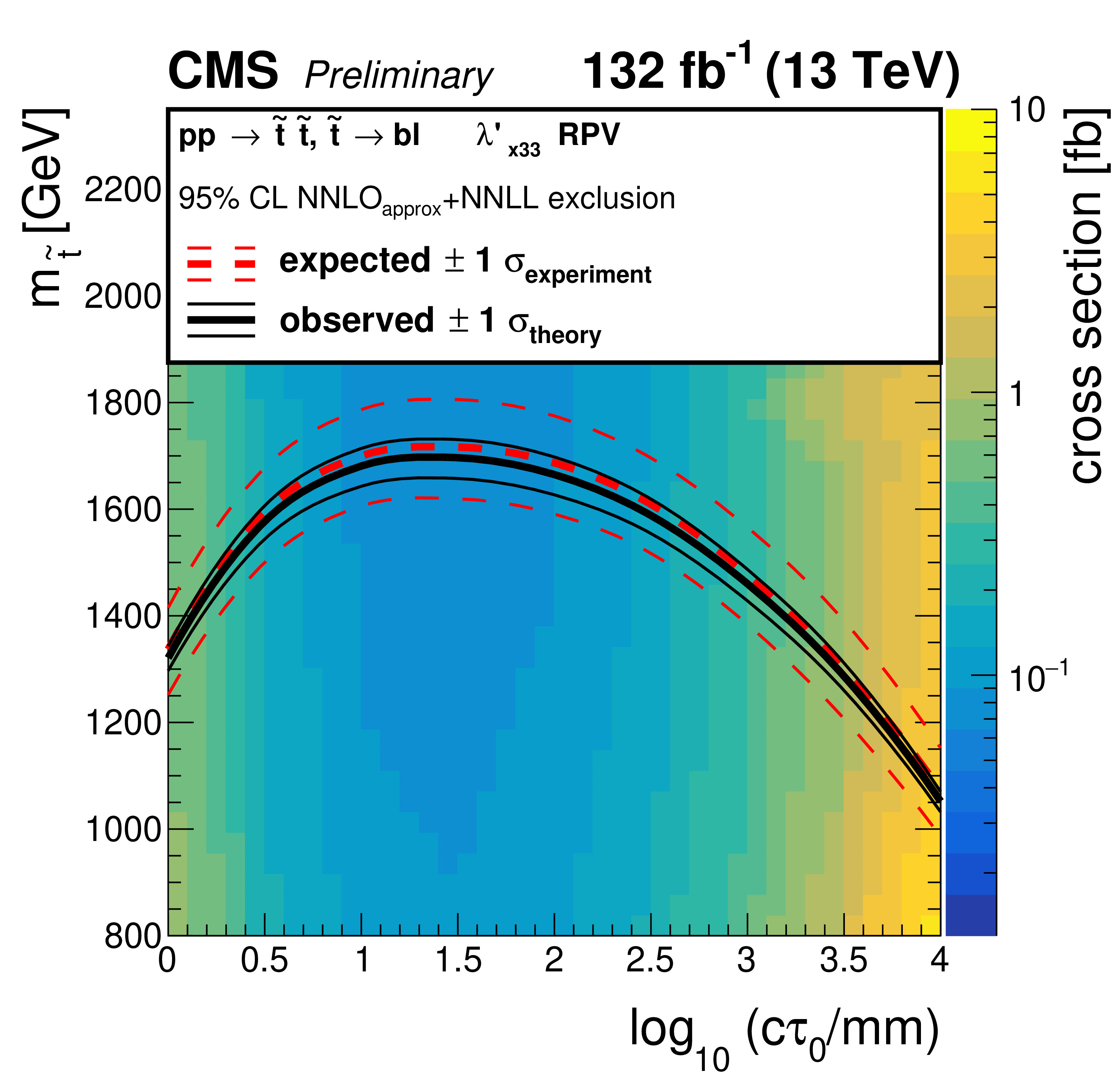
Figure 12:
Left: the expected and observed 95% CL upper limits on the pair production cross section of the long-lived top squarks, assuming a 100% branching fraction for $\tilde{\mathrm{t}} \to \mathrm{b} \ell $ decays, with equal branching fractions for e, $\mu $, and $\tau $. The horizontal lines indicate the NNLO$_{approx}$+NNLL top squark pair production cross sections for $m_{\tilde{\mathrm{t}}} = $ 1600 GeV and $m_{\tilde{\mathrm{t}}} = $ 1000 GeV, as well as their variations due to the uncertainties in the choices of renormalization scales, factorization scales, and PDF sets. The solid (dashed) lines represent the observed (median expected) limits, the bands show the regions containing 68% of the distributions of the expected limits under the background-only hypothesis. Right: the expected and observed 95% CL limits for the long-lived top squark model in the mass-lifetime plane, assuming a 100% branching fraction for $\tilde{\mathrm{t}} \to \mathrm{b} \ell $ decays, based on the NNLO$_{approx}$+NNLL calculation of the top squark pair production cross section at $\sqrt {s} = $ 13 TeV. The thick solid black (dashed red) line represents the observed (median expected) limits at 95% CL . The thin red lines indicate the region containing 68% of the distribution of the expected limits under the background-only hypothesis. The thin black lines represent the change in the observed limit due to the variation of the signal cross sections within the theoretical uncertainties. |
png pdf |
Figure 12-a:
Left: the expected and observed 95% CL upper limits on the pair production cross section of the long-lived top squarks, assuming a 100% branching fraction for $\tilde{\mathrm{t}} \to \mathrm{b} \ell $ decays, with equal branching fractions for e, $\mu $, and $\tau $. The horizontal lines indicate the NNLO$_{approx}$+NNLL top squark pair production cross sections for $m_{\tilde{\mathrm{t}}} = $ 1600 GeV and $m_{\tilde{\mathrm{t}}} = $ 1000 GeV, as well as their variations due to the uncertainties in the choices of renormalization scales, factorization scales, and PDF sets. The solid (dashed) lines represent the observed (median expected) limits, the bands show the regions containing 68% of the distributions of the expected limits under the background-only hypothesis. Right: the expected and observed 95% CL limits for the long-lived top squark model in the mass-lifetime plane, assuming a 100% branching fraction for $\tilde{\mathrm{t}} \to \mathrm{b} \ell $ decays, based on the NNLO$_{approx}$+NNLL calculation of the top squark pair production cross section at $\sqrt {s} = $ 13 TeV. The thick solid black (dashed red) line represents the observed (median expected) limits at 95% CL . The thin red lines indicate the region containing 68% of the distribution of the expected limits under the background-only hypothesis. The thin black lines represent the change in the observed limit due to the variation of the signal cross sections within the theoretical uncertainties. |
png pdf |
Figure 12-b:
Left: the expected and observed 95% CL upper limits on the pair production cross section of the long-lived top squarks, assuming a 100% branching fraction for $\tilde{\mathrm{t}} \to \mathrm{b} \ell $ decays, with equal branching fractions for e, $\mu $, and $\tau $. The horizontal lines indicate the NNLO$_{approx}$+NNLL top squark pair production cross sections for $m_{\tilde{\mathrm{t}}} = $ 1600 GeV and $m_{\tilde{\mathrm{t}}} = $ 1000 GeV, as well as their variations due to the uncertainties in the choices of renormalization scales, factorization scales, and PDF sets. The solid (dashed) lines represent the observed (median expected) limits, the bands show the regions containing 68% of the distributions of the expected limits under the background-only hypothesis. Right: the expected and observed 95% CL limits for the long-lived top squark model in the mass-lifetime plane, assuming a 100% branching fraction for $\tilde{\mathrm{t}} \to \mathrm{b} \ell $ decays, based on the NNLO$_{approx}$+NNLL calculation of the top squark pair production cross section at $\sqrt {s} = $ 13 TeV. The thick solid black (dashed red) line represents the observed (median expected) limits at 95% CL . The thin red lines indicate the region containing 68% of the distribution of the expected limits under the background-only hypothesis. The thin black lines represent the change in the observed limit due to the variation of the signal cross sections within the theoretical uncertainties. |
png pdf |
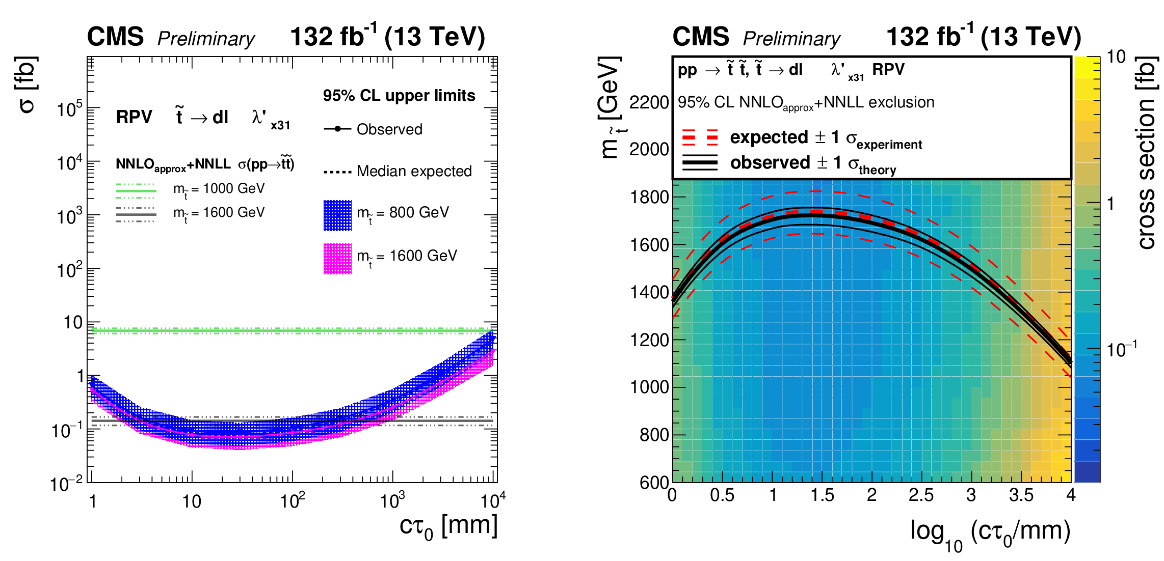
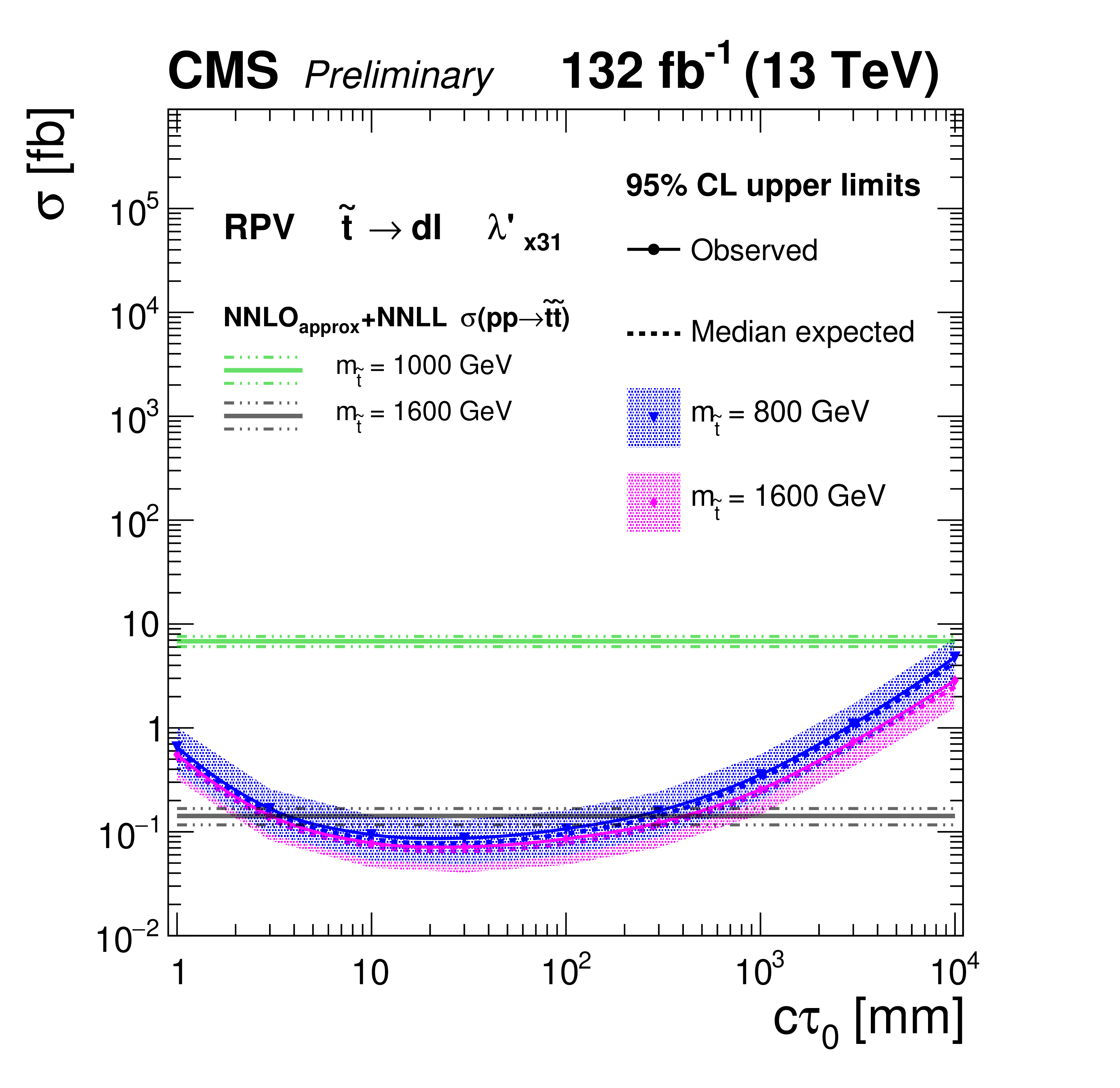
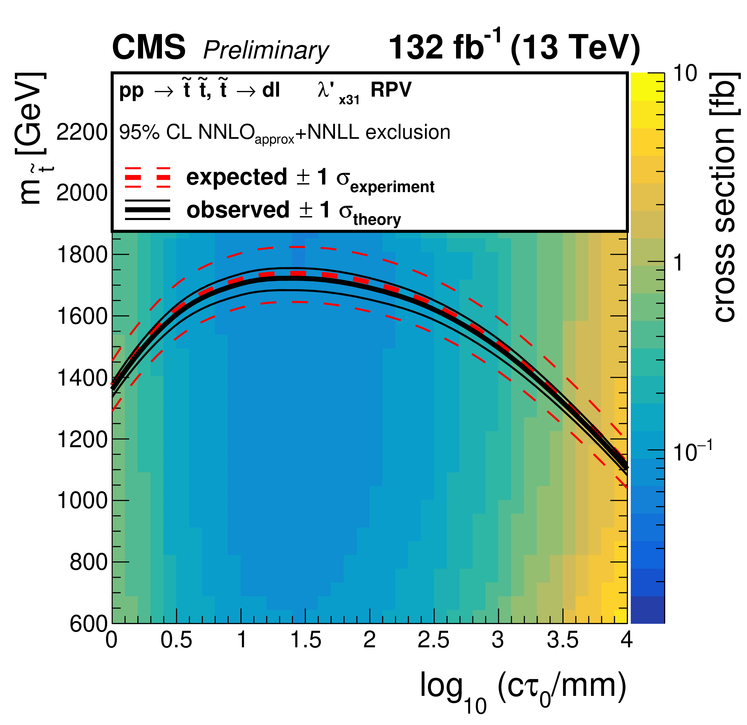
Figure 13:
Left: the expected and observed 95% CL upper limits on the pair production cross section of the long-lived top squarks, assuming a 100% branching fraction for $\tilde{\mathrm{t}} \to \mathrm{d} \ell $ decays, with equal branching fractions for e, $\mu $, and $\tau $. The horizontal lines indicate the NNLO$_{approx}$+NNLL top squark pair production cross sections for $m_{\tilde{\mathrm{t}}} = $ 1600 GeV and $m_{\tilde{\mathrm{t}}} = $ 1000 GeV, as well as their variations due to the uncertainties in the choices of renormalization scales, factorization scales, and PDF sets. The solid (dashed) lines represent the observed (median expected) limits, the bands show the regions containing 68% of the distributions of the expected limits under the background-only hypothesis. Right: the expected and observed 95% CL limits for the long-lived top squark model in the mass-lifetime plane, assuming a 100% branching fraction for $\tilde{\mathrm{t}} \to \mathrm{d} \ell $ decays, based on the NNLO$_{approx}$+NNLL calculation of the top squark pair production cross section at $\sqrt {s} = $ 13 TeV. The thick solid black (dashed red) line represents the observed (median expected) limits at 95% CL . The thin red lines indicate the region containing 68% of the distribution of the expected limits under the background-only hypothesis. The thin black lines represent the change in the observed limit due to the variation of the signal cross sections within the theoretical uncertainties. |
png pdf |
Figure 13-a:
Left: the expected and observed 95% CL upper limits on the pair production cross section of the long-lived top squarks, assuming a 100% branching fraction for $\tilde{\mathrm{t}} \to \mathrm{d} \ell $ decays, with equal branching fractions for e, $\mu $, and $\tau $. The horizontal lines indicate the NNLO$_{approx}$+NNLL top squark pair production cross sections for $m_{\tilde{\mathrm{t}}} = $ 1600 GeV and $m_{\tilde{\mathrm{t}}} = $ 1000 GeV, as well as their variations due to the uncertainties in the choices of renormalization scales, factorization scales, and PDF sets. The solid (dashed) lines represent the observed (median expected) limits, the bands show the regions containing 68% of the distributions of the expected limits under the background-only hypothesis. Right: the expected and observed 95% CL limits for the long-lived top squark model in the mass-lifetime plane, assuming a 100% branching fraction for $\tilde{\mathrm{t}} \to \mathrm{d} \ell $ decays, based on the NNLO$_{approx}$+NNLL calculation of the top squark pair production cross section at $\sqrt {s} = $ 13 TeV. The thick solid black (dashed red) line represents the observed (median expected) limits at 95% CL . The thin red lines indicate the region containing 68% of the distribution of the expected limits under the background-only hypothesis. The thin black lines represent the change in the observed limit due to the variation of the signal cross sections within the theoretical uncertainties. |
png pdf |
Figure 13-b:
Left: the expected and observed 95% CL upper limits on the pair production cross section of the long-lived top squarks, assuming a 100% branching fraction for $\tilde{\mathrm{t}} \to \mathrm{d} \ell $ decays, with equal branching fractions for e, $\mu $, and $\tau $. The horizontal lines indicate the NNLO$_{approx}$+NNLL top squark pair production cross sections for $m_{\tilde{\mathrm{t}}} = $ 1600 GeV and $m_{\tilde{\mathrm{t}}} = $ 1000 GeV, as well as their variations due to the uncertainties in the choices of renormalization scales, factorization scales, and PDF sets. The solid (dashed) lines represent the observed (median expected) limits, the bands show the regions containing 68% of the distributions of the expected limits under the background-only hypothesis. Right: the expected and observed 95% CL limits for the long-lived top squark model in the mass-lifetime plane, assuming a 100% branching fraction for $\tilde{\mathrm{t}} \to \mathrm{d} \ell $ decays, based on the NNLO$_{approx}$+NNLL calculation of the top squark pair production cross section at $\sqrt {s} = $ 13 TeV. The thick solid black (dashed red) line represents the observed (median expected) limits at 95% CL . The thin red lines indicate the region containing 68% of the distribution of the expected limits under the background-only hypothesis. The thin black lines represent the change in the observed limit due to the variation of the signal cross sections within the theoretical uncertainties. |

png pdf |
Figure 14:
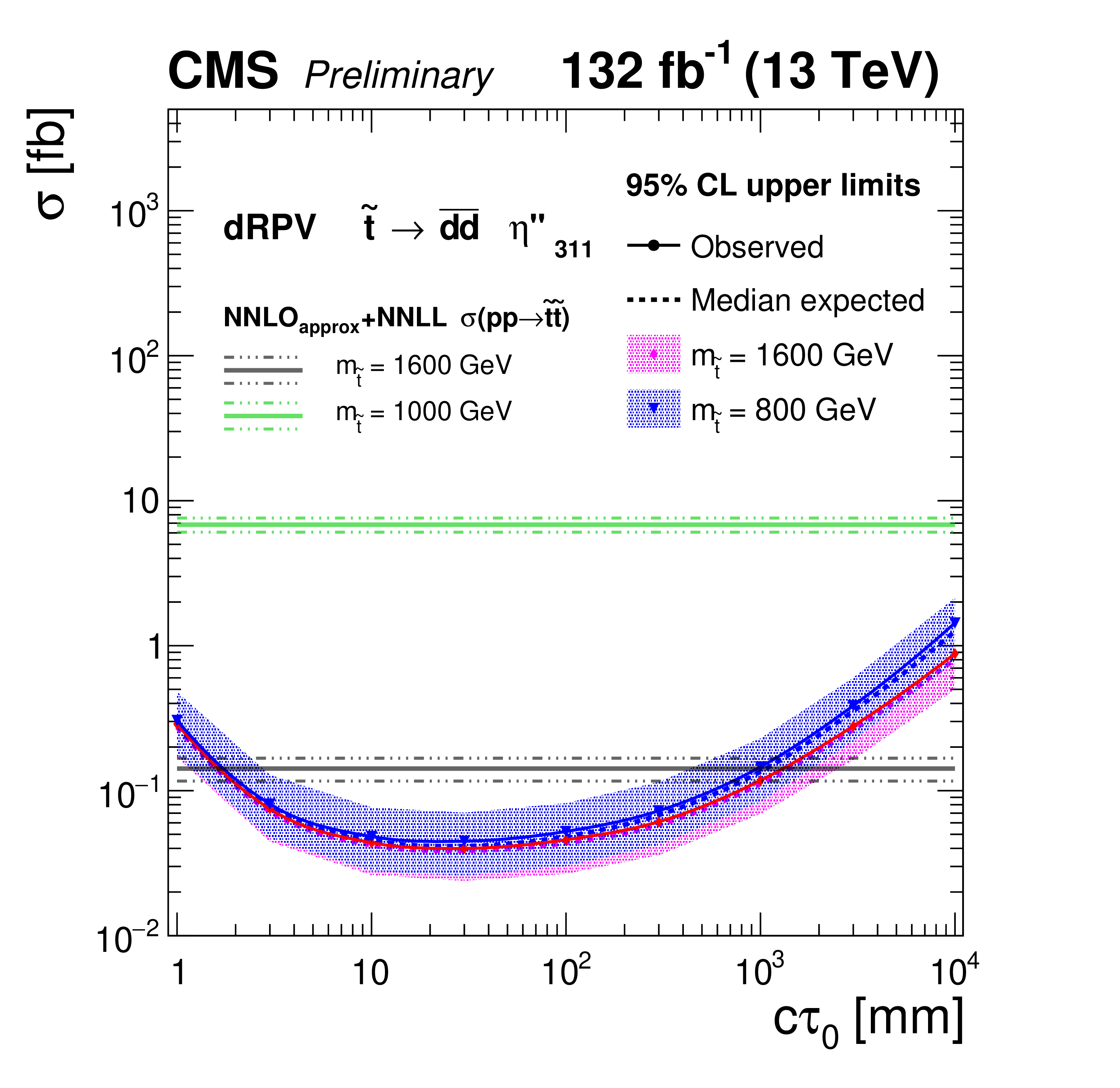
Left: the expected and observed 95% CL upper limits on the pair production cross section of the long-lived top squarks, assuming a 100% branching fraction for $\tilde{\mathrm{t}} \to \mathrm{\bar{d}} \mathrm{\bar{d}} $ decays. The horizontal lines indicate the NNLO$_{approx}$+NNLL top squark pair production cross sections for $m_{\tilde{\mathrm{t}}} = $ 1600 GeV and $m_{\tilde{\mathrm{t}}} = $ 1000 GeV, as well as their variations due to the uncertainties in the choices of renormalization scales, factorization scales, and PDF sets. The solid (dashed) lines represent the observed (median expected) limits, the bands show the regions containing 68% of the distributions of the expected limits under the background-only hypothesis. Right: the expected and observed 95% CL limits for the long-lived top squark model in the mass-lifetime plane, assuming a 100% branching fraction for $\tilde{\mathrm{t}} \to \mathrm{\bar{d}} \mathrm{\bar{d}} $ decays, based on the NNLO$_{approx}$+NNLL calculation of the top squark pair production cross section at $\sqrt {s} = $ 13 TeV. The thick solid black (dashed red) line represents the observed (median expected) limits at 95% CL . The thin red lines indicate the region containing 68% of the distribution of the expected limits under the background-only hypothesis. The thin black lines represent the change in the observed limit due to the variation of the signal cross sections within the theoretical uncertainties. |
png pdf |
Figure 14-a:
Left: the expected and observed 95% CL upper limits on the pair production cross section of the long-lived top squarks, assuming a 100% branching fraction for $\tilde{\mathrm{t}} \to \mathrm{\bar{d}} \mathrm{\bar{d}} $ decays. The horizontal lines indicate the NNLO$_{approx}$+NNLL top squark pair production cross sections for $m_{\tilde{\mathrm{t}}} = $ 1600 GeV and $m_{\tilde{\mathrm{t}}} = $ 1000 GeV, as well as their variations due to the uncertainties in the choices of renormalization scales, factorization scales, and PDF sets. The solid (dashed) lines represent the observed (median expected) limits, the bands show the regions containing 68% of the distributions of the expected limits under the background-only hypothesis. Right: the expected and observed 95% CL limits for the long-lived top squark model in the mass-lifetime plane, assuming a 100% branching fraction for $\tilde{\mathrm{t}} \to \mathrm{\bar{d}} \mathrm{\bar{d}} $ decays, based on the NNLO$_{approx}$+NNLL calculation of the top squark pair production cross section at $\sqrt {s} = $ 13 TeV. The thick solid black (dashed red) line represents the observed (median expected) limits at 95% CL . The thin red lines indicate the region containing 68% of the distribution of the expected limits under the background-only hypothesis. The thin black lines represent the change in the observed limit due to the variation of the signal cross sections within the theoretical uncertainties. |

png pdf |
Figure 14-b:
Left: the expected and observed 95% CL upper limits on the pair production cross section of the long-lived top squarks, assuming a 100% branching fraction for $\tilde{\mathrm{t}} \to \mathrm{\bar{d}} \mathrm{\bar{d}} $ decays. The horizontal lines indicate the NNLO$_{approx}$+NNLL top squark pair production cross sections for $m_{\tilde{\mathrm{t}}} = $ 1600 GeV and $m_{\tilde{\mathrm{t}}} = $ 1000 GeV, as well as their variations due to the uncertainties in the choices of renormalization scales, factorization scales, and PDF sets. The solid (dashed) lines represent the observed (median expected) limits, the bands show the regions containing 68% of the distributions of the expected limits under the background-only hypothesis. Right: the expected and observed 95% CL limits for the long-lived top squark model in the mass-lifetime plane, assuming a 100% branching fraction for $\tilde{\mathrm{t}} \to \mathrm{\bar{d}} \mathrm{\bar{d}} $ decays, based on the NNLO$_{approx}$+NNLL calculation of the top squark pair production cross section at $\sqrt {s} = $ 13 TeV. The thick solid black (dashed red) line represents the observed (median expected) limits at 95% CL . The thin red lines indicate the region containing 68% of the distribution of the expected limits under the background-only hypothesis. The thin black lines represent the change in the observed limit due to the variation of the signal cross sections within the theoretical uncertainties. |
png pdf |
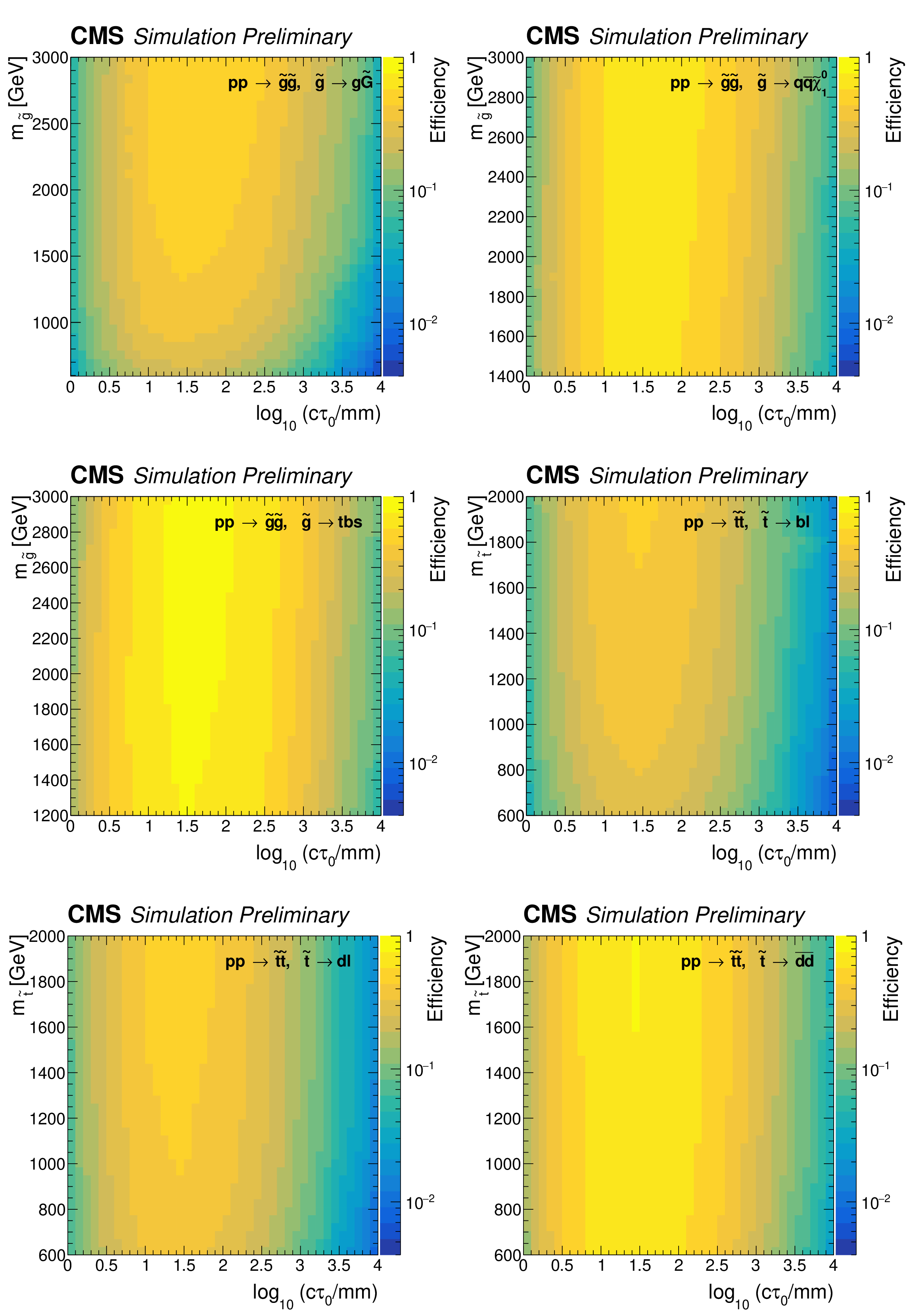
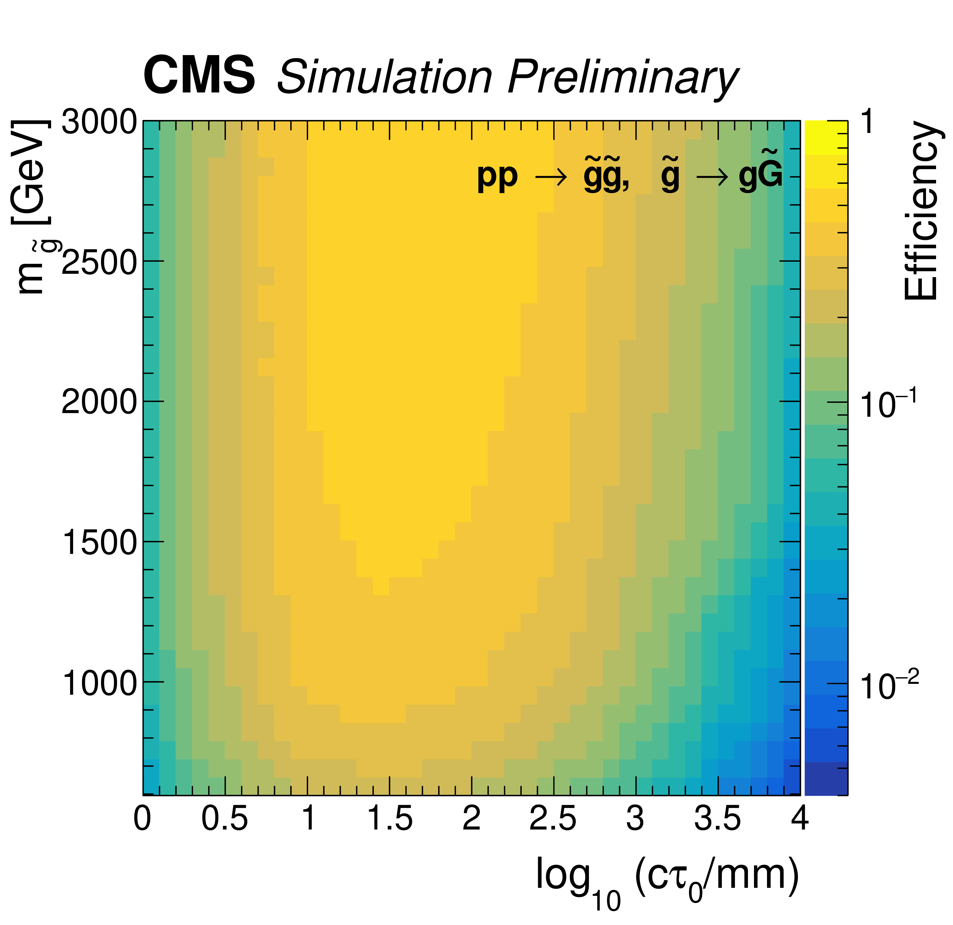
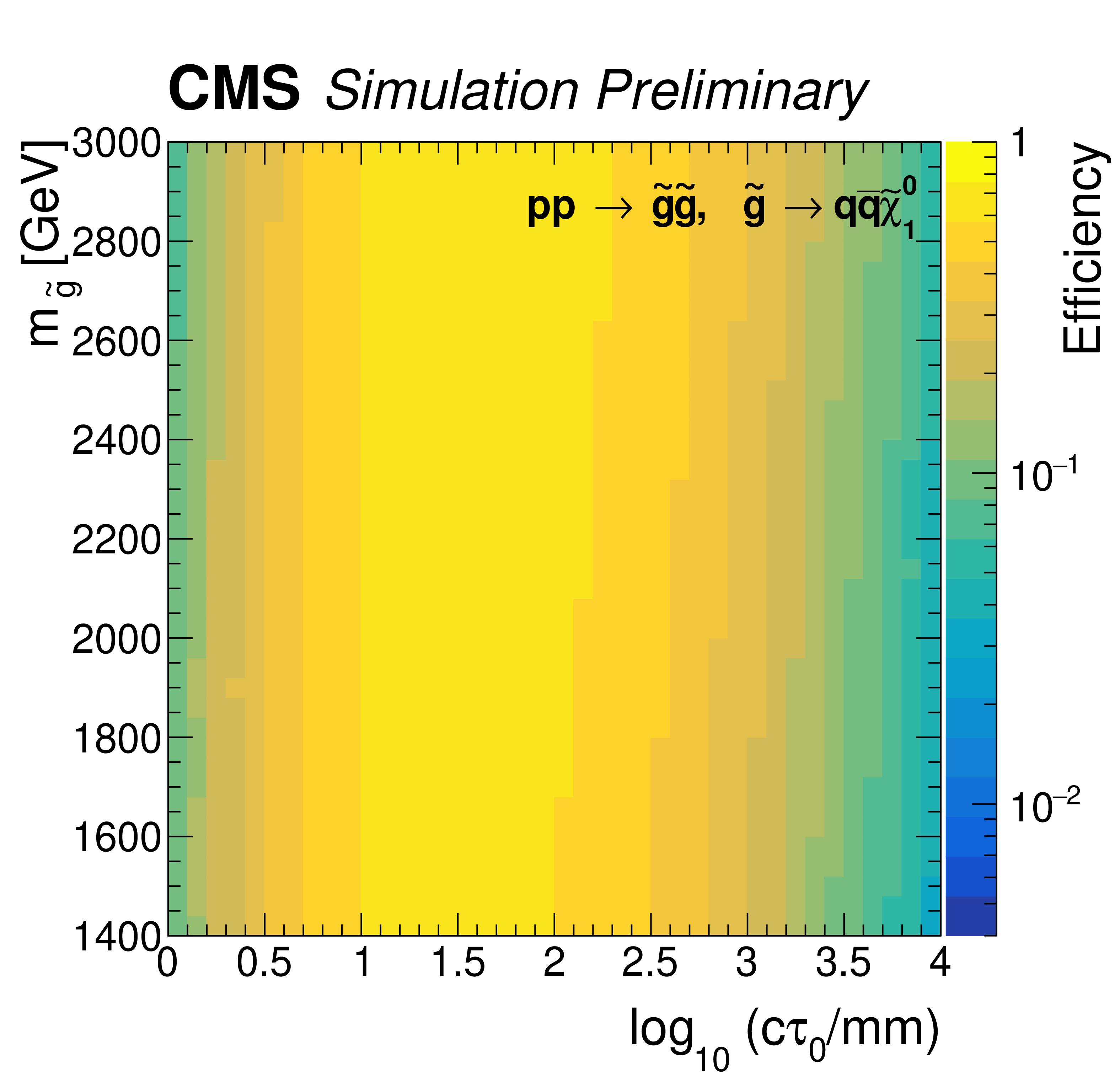
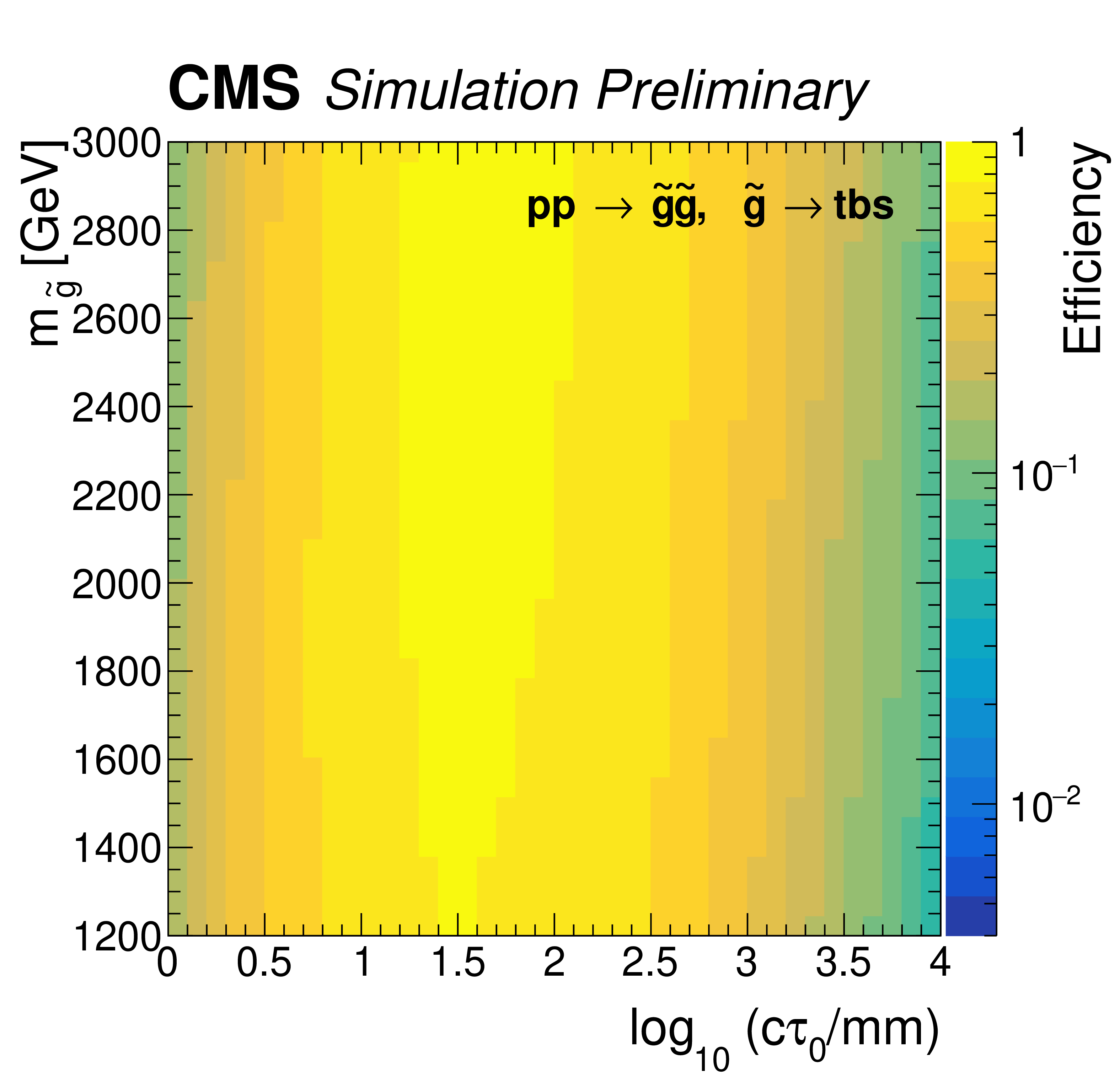
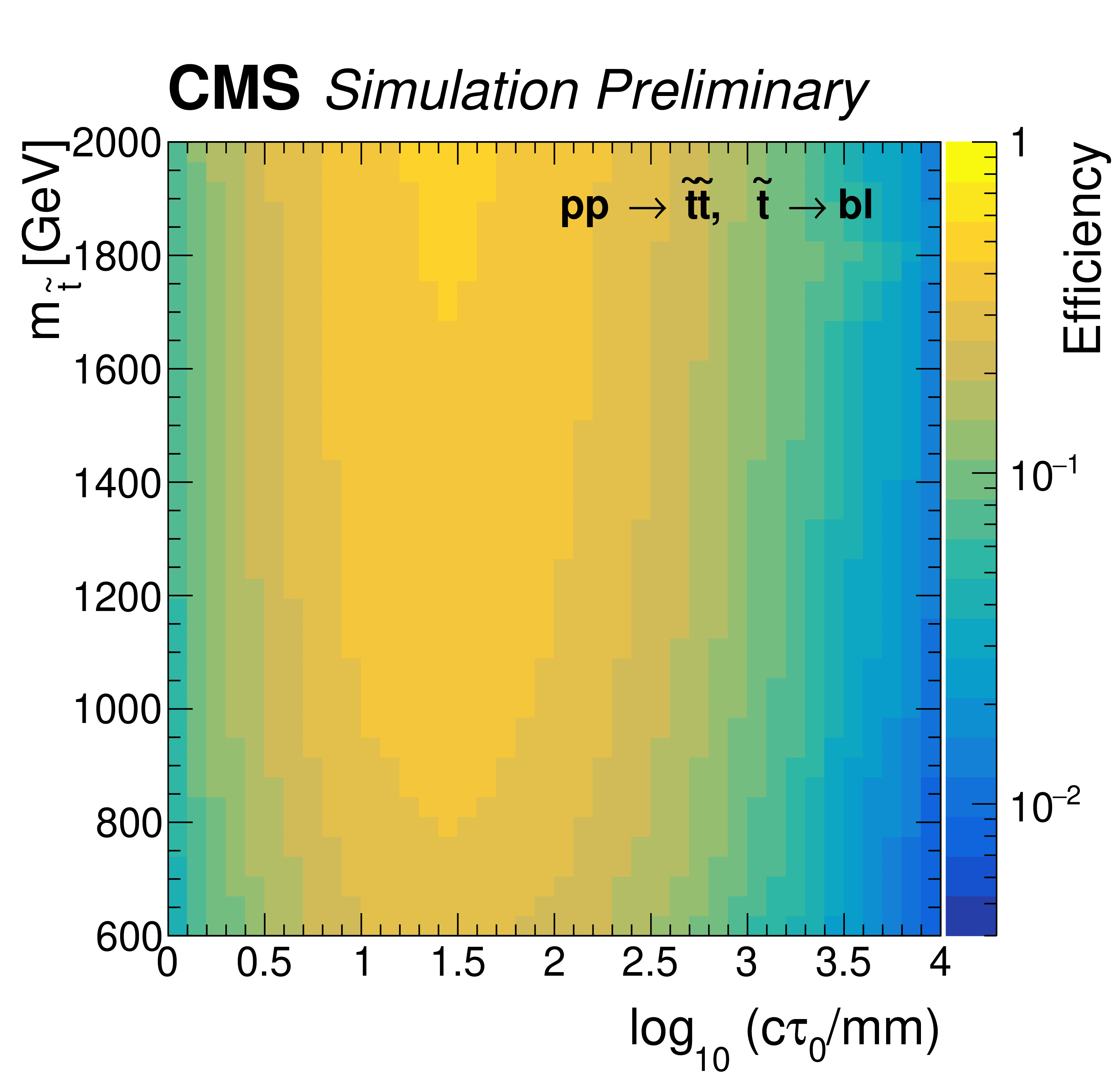
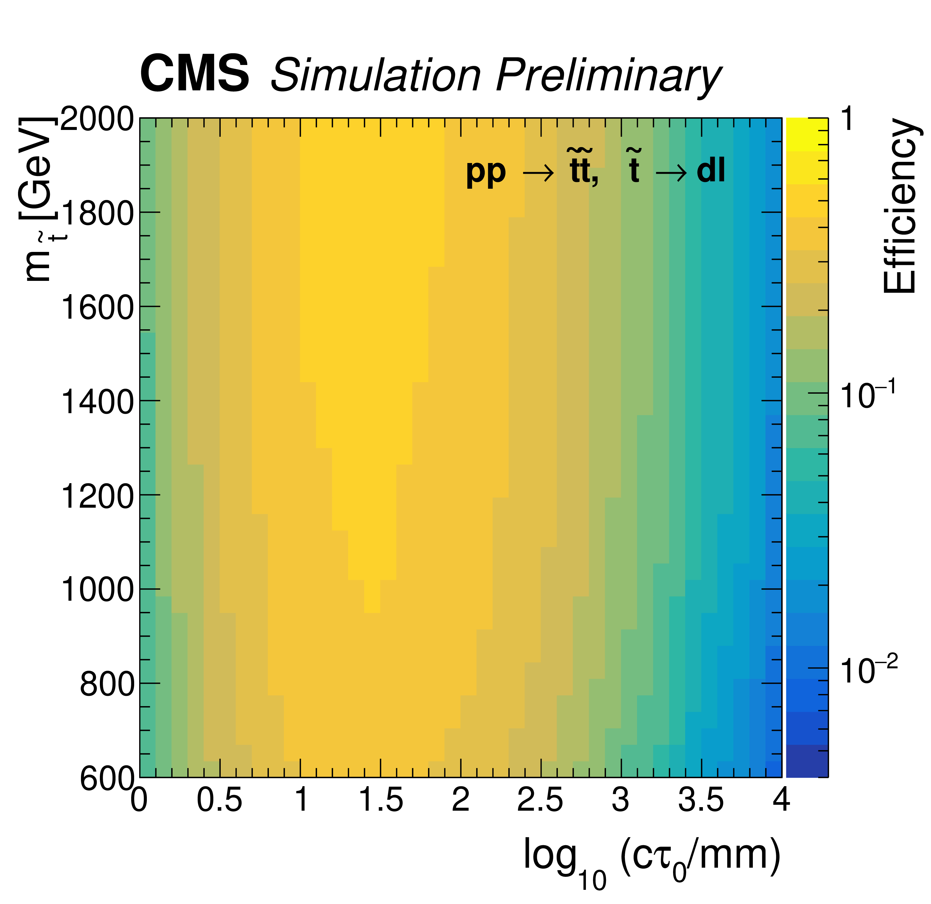
Figure 15:
The signal efficiencies as functions of the long-lived particle mass and mean proper decay lengths in 2017 and 2018, for ${\mathrm{\tilde{g}}} \to \mathrm{g} \tilde{\mathrm{G}} $ model (top left), ${\mathrm{\tilde{g}}} \to \mathrm{q} \mathrm{\bar{q}} \tilde{\chi}^{0}_{1}$ model (top right), ${\mathrm{\tilde{g}}} \to \mathrm{t} \mathrm{b} \mathrm{s} $ model (middle left), $\tilde{\mathrm{t}} \to \mathrm{b} \ell $ model (middle right), $\tilde{\mathrm{t}} \to \mathrm{d} \ell $ model (bottom left), and $\tilde{\mathrm{t}} \to \mathrm{\bar{d}} \mathrm{\bar{d}} $ model (bottom right). |
png pdf |
Figure 15-a:
The signal efficiencies as functions of the long-lived particle mass and mean proper decay lengths in 2017 and 2018, for ${\mathrm{\tilde{g}}} \to \mathrm{g} \tilde{\mathrm{G}} $ model (top left), ${\mathrm{\tilde{g}}} \to \mathrm{q} \mathrm{\bar{q}} \tilde{\chi}^{0}_{1}$ model (top right), ${\mathrm{\tilde{g}}} \to \mathrm{t} \mathrm{b} \mathrm{s} $ model (middle left), $\tilde{\mathrm{t}} \to \mathrm{b} \ell $ model (middle right), $\tilde{\mathrm{t}} \to \mathrm{d} \ell $ model (bottom left), and $\tilde{\mathrm{t}} \to \mathrm{\bar{d}} \mathrm{\bar{d}} $ model (bottom right). |
png pdf |
Figure 15-b:
The signal efficiencies as functions of the long-lived particle mass and mean proper decay lengths in 2017 and 2018, for ${\mathrm{\tilde{g}}} \to \mathrm{g} \tilde{\mathrm{G}} $ model (top left), ${\mathrm{\tilde{g}}} \to \mathrm{q} \mathrm{\bar{q}} \tilde{\chi}^{0}_{1}$ model (top right), ${\mathrm{\tilde{g}}} \to \mathrm{t} \mathrm{b} \mathrm{s} $ model (middle left), $\tilde{\mathrm{t}} \to \mathrm{b} \ell $ model (middle right), $\tilde{\mathrm{t}} \to \mathrm{d} \ell $ model (bottom left), and $\tilde{\mathrm{t}} \to \mathrm{\bar{d}} \mathrm{\bar{d}} $ model (bottom right). |
png pdf |
Figure 15-c:
The signal efficiencies as functions of the long-lived particle mass and mean proper decay lengths in 2017 and 2018, for ${\mathrm{\tilde{g}}} \to \mathrm{g} \tilde{\mathrm{G}} $ model (top left), ${\mathrm{\tilde{g}}} \to \mathrm{q} \mathrm{\bar{q}} \tilde{\chi}^{0}_{1}$ model (top right), ${\mathrm{\tilde{g}}} \to \mathrm{t} \mathrm{b} \mathrm{s} $ model (middle left), $\tilde{\mathrm{t}} \to \mathrm{b} \ell $ model (middle right), $\tilde{\mathrm{t}} \to \mathrm{d} \ell $ model (bottom left), and $\tilde{\mathrm{t}} \to \mathrm{\bar{d}} \mathrm{\bar{d}} $ model (bottom right). |
png pdf |
Figure 15-d:
The signal efficiencies as functions of the long-lived particle mass and mean proper decay lengths in 2017 and 2018, for ${\mathrm{\tilde{g}}} \to \mathrm{g} \tilde{\mathrm{G}} $ model (top left), ${\mathrm{\tilde{g}}} \to \mathrm{q} \mathrm{\bar{q}} \tilde{\chi}^{0}_{1}$ model (top right), ${\mathrm{\tilde{g}}} \to \mathrm{t} \mathrm{b} \mathrm{s} $ model (middle left), $\tilde{\mathrm{t}} \to \mathrm{b} \ell $ model (middle right), $\tilde{\mathrm{t}} \to \mathrm{d} \ell $ model (bottom left), and $\tilde{\mathrm{t}} \to \mathrm{\bar{d}} \mathrm{\bar{d}} $ model (bottom right). |
png pdf |
Figure 15-e:
The signal efficiencies as functions of the long-lived particle mass and mean proper decay lengths in 2017 and 2018, for ${\mathrm{\tilde{g}}} \to \mathrm{g} \tilde{\mathrm{G}} $ model (top left), ${\mathrm{\tilde{g}}} \to \mathrm{q} \mathrm{\bar{q}} \tilde{\chi}^{0}_{1}$ model (top right), ${\mathrm{\tilde{g}}} \to \mathrm{t} \mathrm{b} \mathrm{s} $ model (middle left), $\tilde{\mathrm{t}} \to \mathrm{b} \ell $ model (middle right), $\tilde{\mathrm{t}} \to \mathrm{d} \ell $ model (bottom left), and $\tilde{\mathrm{t}} \to \mathrm{\bar{d}} \mathrm{\bar{d}} $ model (bottom right). |

png pdf |
Figure 15-f:
The signal efficiencies as functions of the long-lived particle mass and mean proper decay lengths in 2017 and 2018, for ${\mathrm{\tilde{g}}} \to \mathrm{g} \tilde{\mathrm{G}} $ model (top left), ${\mathrm{\tilde{g}}} \to \mathrm{q} \mathrm{\bar{q}} \tilde{\chi}^{0}_{1}$ model (top right), ${\mathrm{\tilde{g}}} \to \mathrm{t} \mathrm{b} \mathrm{s} $ model (middle left), $\tilde{\mathrm{t}} \to \mathrm{b} \ell $ model (middle right), $\tilde{\mathrm{t}} \to \mathrm{d} \ell $ model (bottom left), and $\tilde{\mathrm{t}} \to \mathrm{\bar{d}} \mathrm{\bar{d}} $ model (bottom right). |
| Tables | |
png pdf |
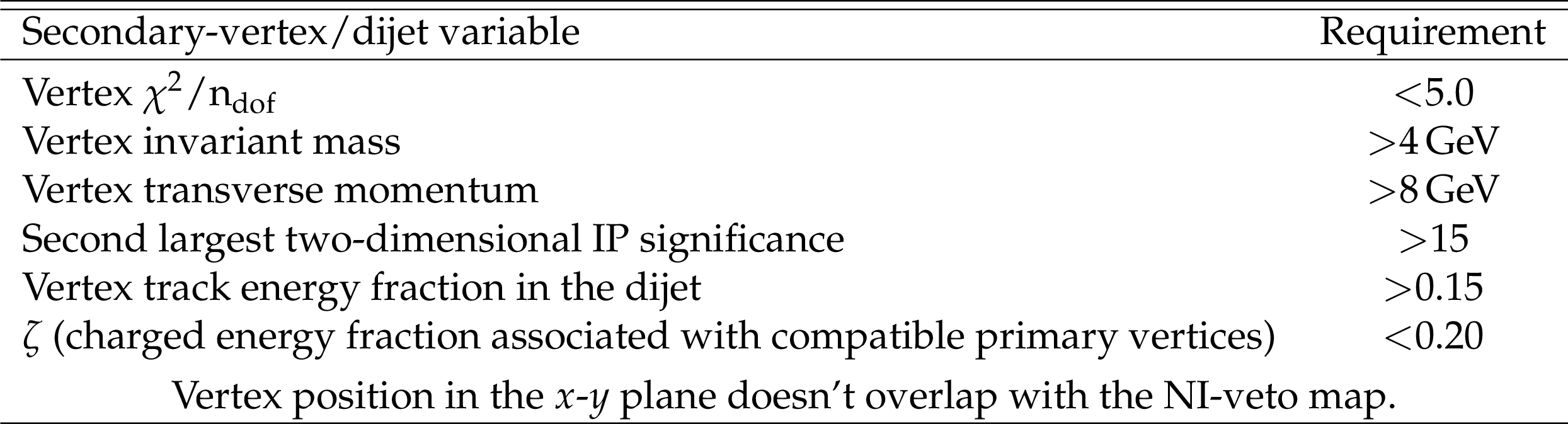
Table 1:
Summary of the preselection criteria. |
png pdf |
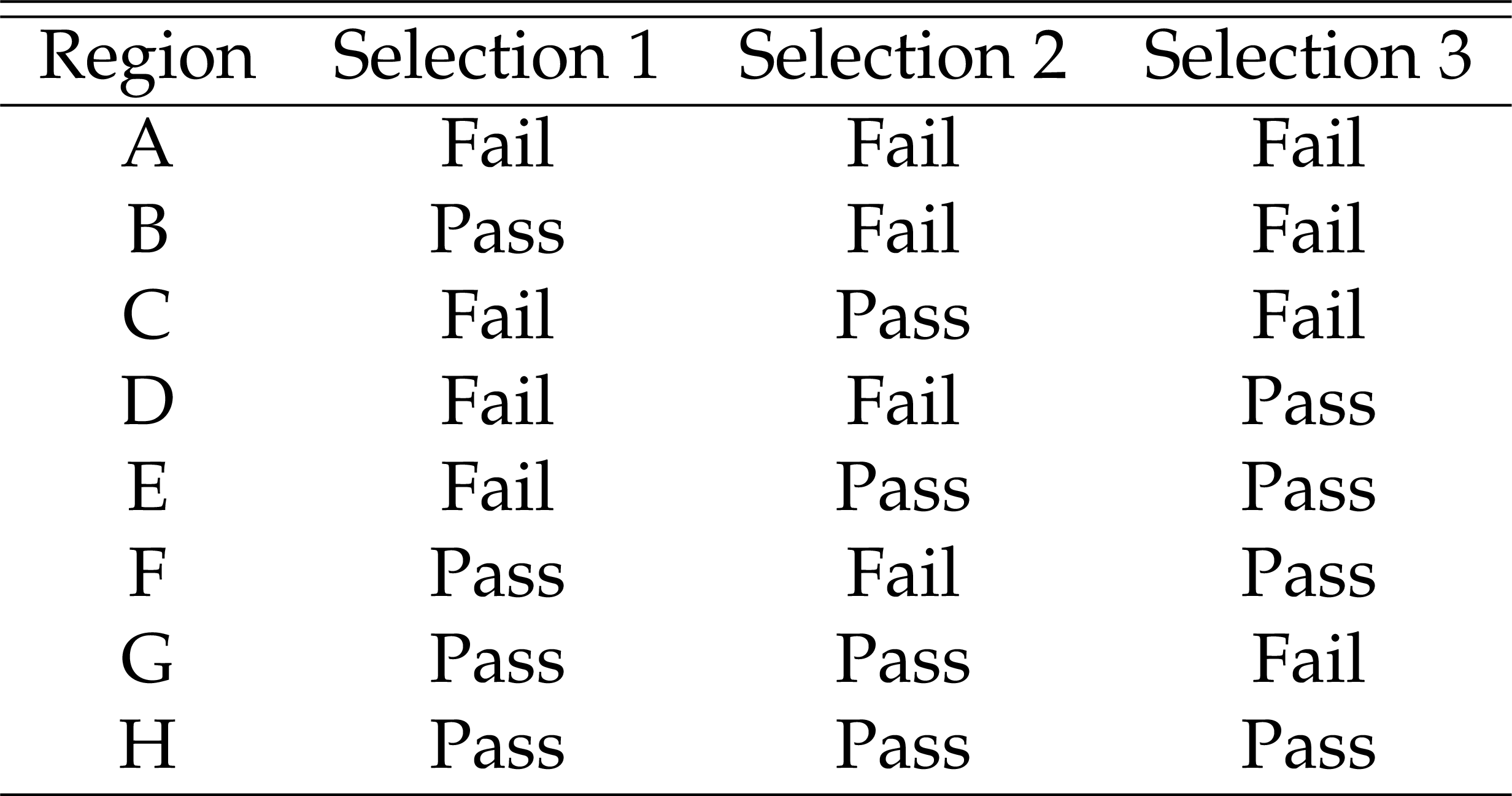
Table 2:
The definition of the different regions used in the background estimation. |
png pdf |
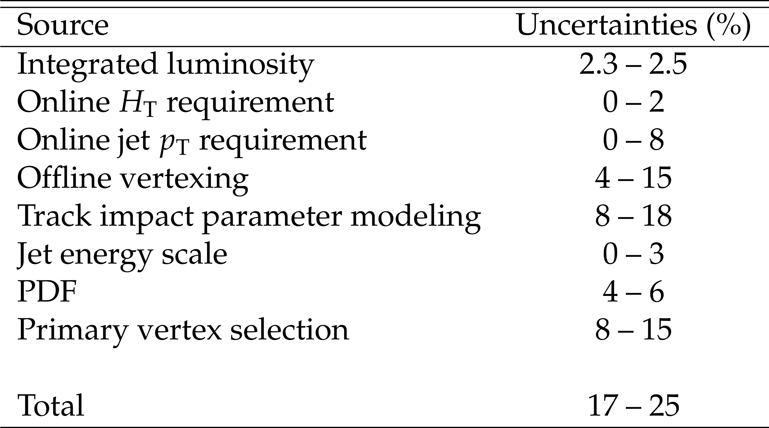
Table 3:
Summary of the systematic uncertainties in signal yields. |
png pdf |
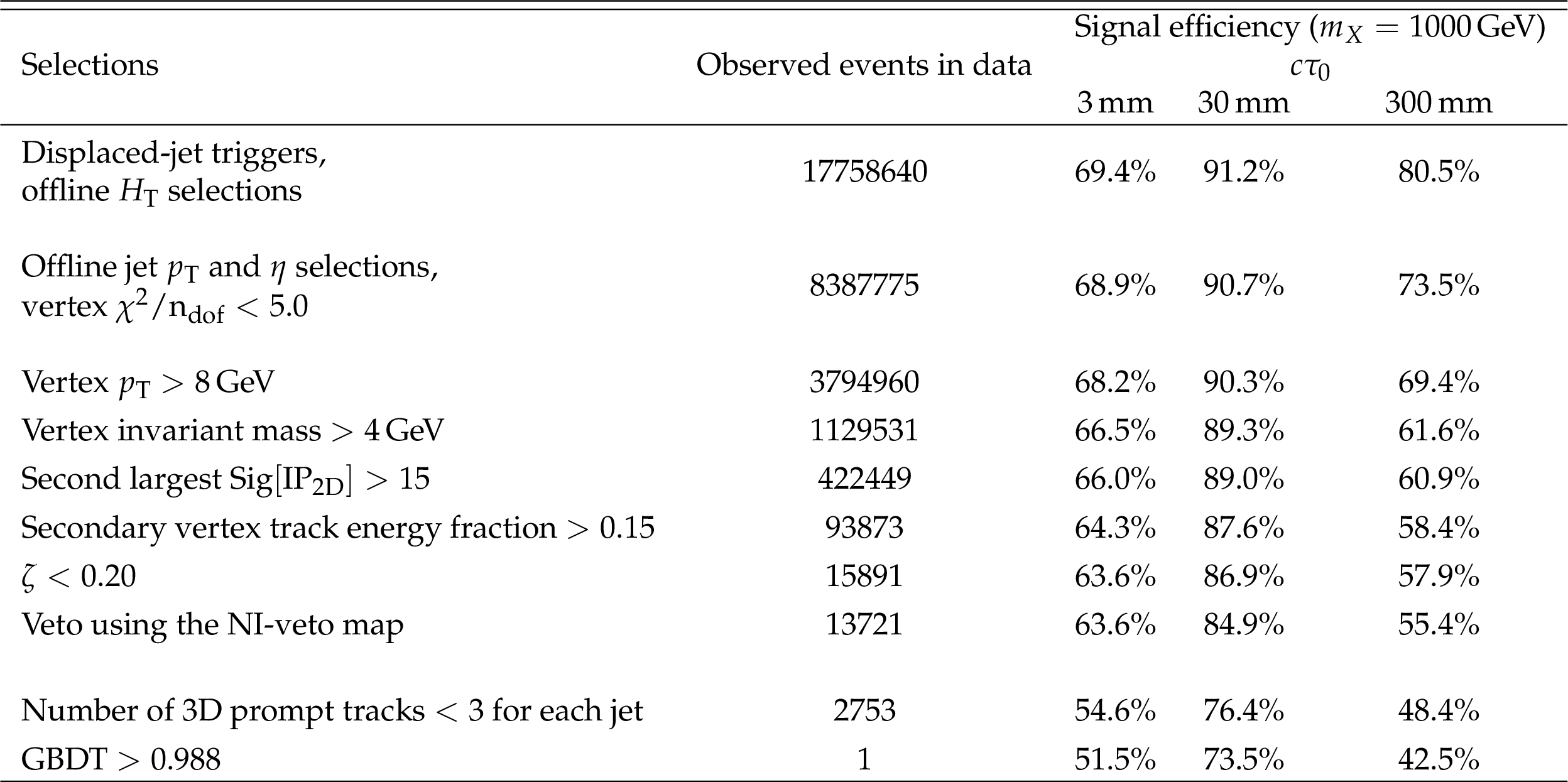
Table 4:
Event yields after different selection requirements applied for data collected in 2017 and 2018. Signal efficiencies for jet-jet model with $m_{\mathrm{X}} = $ 1000 GeV and different $c\tau _{0}$ are also shown for comparison. |
png pdf |
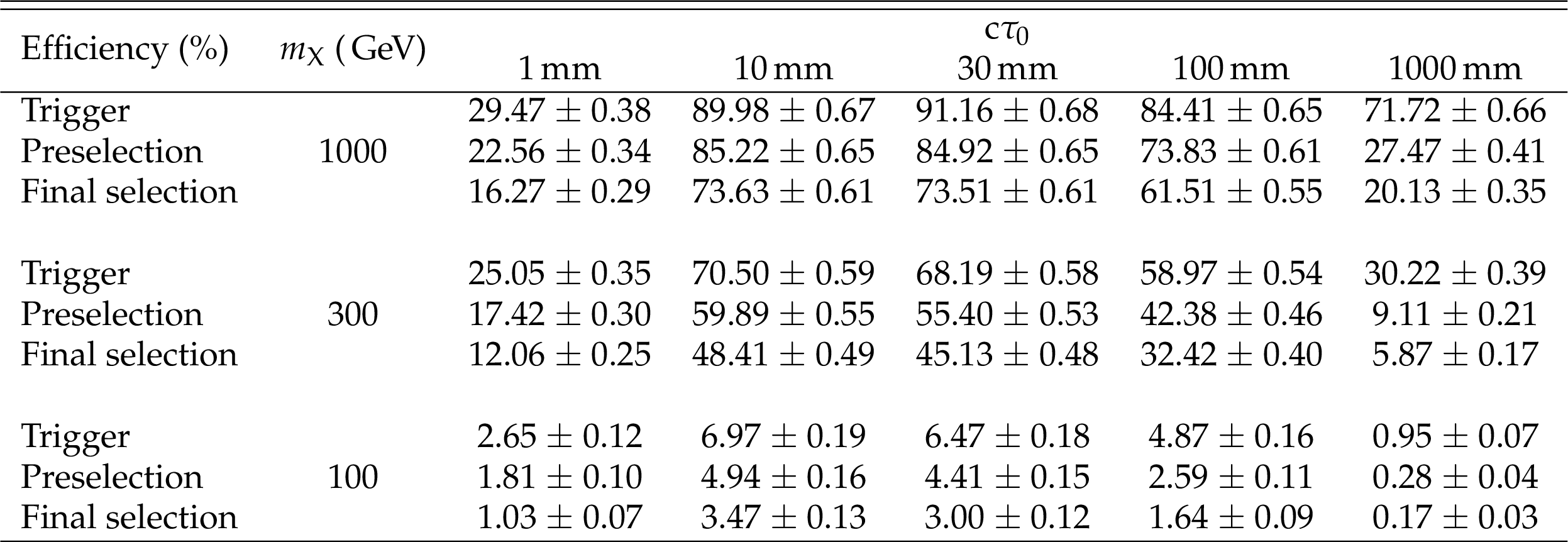
Table 5:
Signal efficiencies (in %) for the jet-jet model in 2017 and 2018 at different proper decay lengths $c\tau _{0}$ and different masses $m_{\mathrm {X}}$. Selection requirements are cumulative from the first row to the last. Uncertainties are statistical only. |
png pdf |
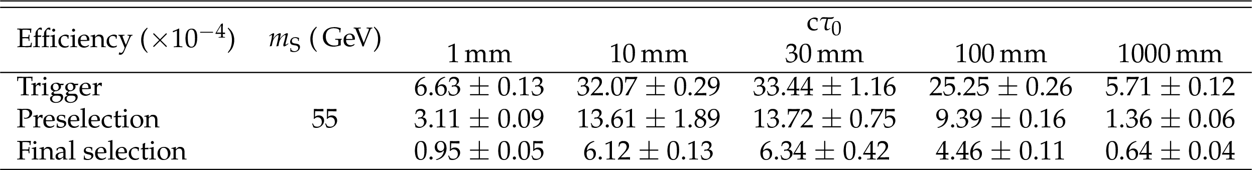
Table 6:
Signal efficiencies (in 10$^{-4}$) for the model where the SM Higgs boson decays to two long-lived scalars S in 2017 and 2018 at different proper decay lengths $c\tau _{0}$ and with $m_{\mathrm {S}} = $ 55 GeV. The long-lived scalars is assumed to decay to a down quark-antiquark pair ($\mathrm {S}\to \mathrm{d} \mathrm{\bar{d}} $). Selection requirements are cumulative from the first row to the last. Uncertainties are statistical only. |
png pdf |
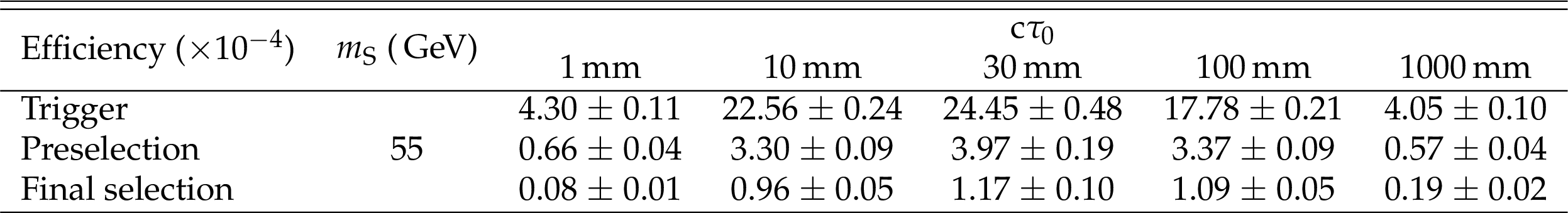
Table 7:
Signal efficiencies (in 10$^{-4}$) for the model where the SM Higgs boson decays to two long-lived scalars S in 2017 and 2018 at different proper decay lengths $c\tau _{0}$ and with $m_{\mathrm {S}} = $ 55 GeV. The long-lived scalar is assumed to decay to a bottom quark-antiquark pair ($\mathrm {S}\to \mathrm{b} \mathrm{\bar{b}} $). Selection requirements are cumulative from the first row to the last. Uncertainties are statistical only. |
png pdf |
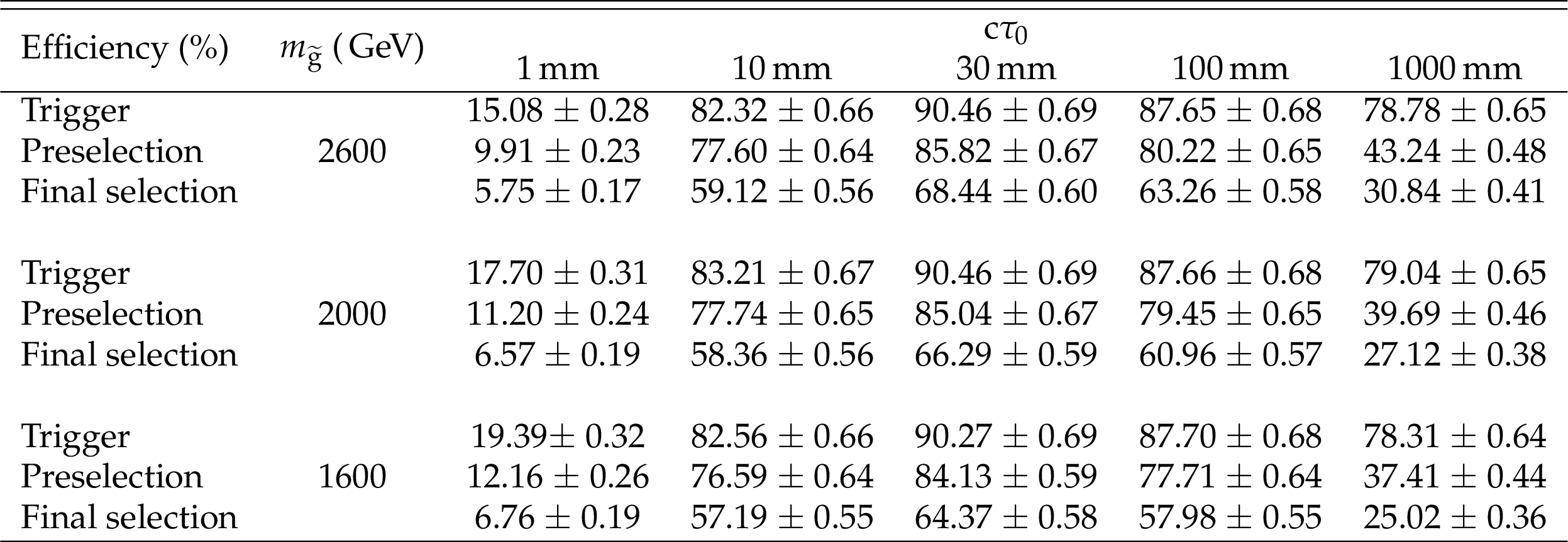
Table 8:
Signal efficiencies (in %) for the ${\mathrm{\tilde{g}}} \to \mathrm{g} \tilde{\mathrm{G}} $ model in 2017 and 2018 at different proper decay lengths $c\tau _{0}$ and different masses $m_{\mathrm {{\mathrm{\tilde{g}}}}}$. Selection requirements are cumulative from the first row to the last. Uncertainties are statistical only. |
png pdf |
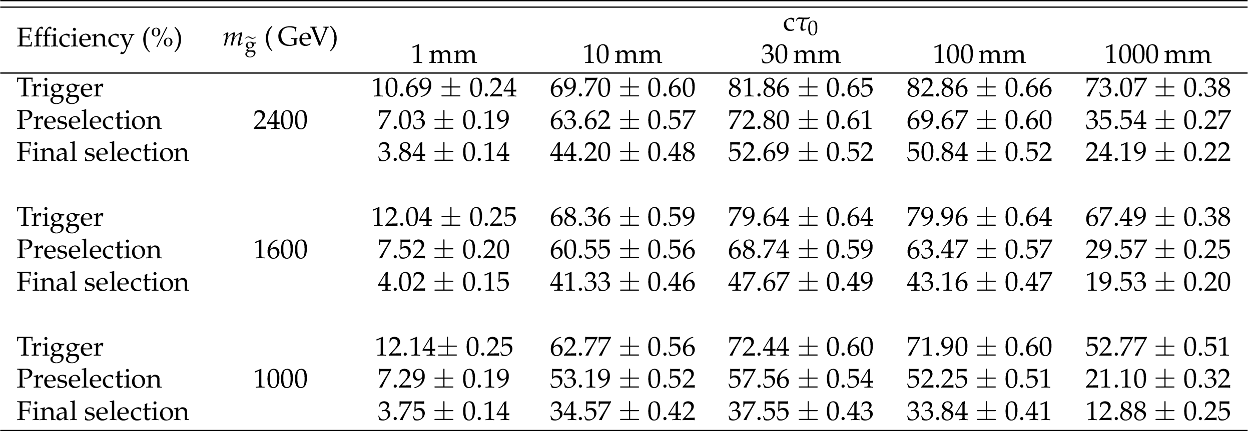
Table 9:
Signal efficiencies (in %) for the ${\mathrm{\tilde{g}}} \to \mathrm{q} \mathrm{\bar{q}} \tilde{\chi}^{0}_{1}$ model ($m_{\tilde{\chi}^{0}_{1}} = $ 100 GeV) in 2017 and 2018 at different proper decay lengths $c\tau _{0}$ and different masses $m_{\mathrm {{\mathrm{\tilde{g}}}}}$. Selection requirements are cumulative from the first row to the last. Uncertainties are statistical only. |
png pdf |
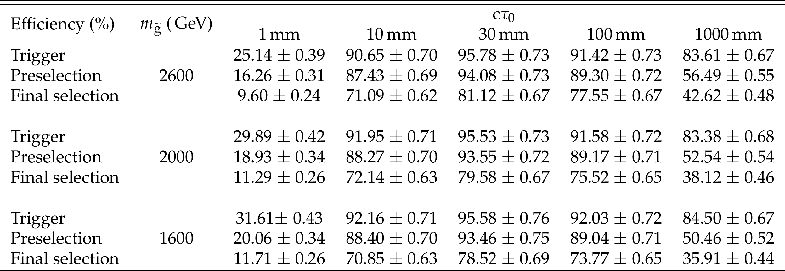
Table 10:
Signal efficiencies (in %) for the ${\mathrm{\tilde{g}}} \to \mathrm{t} \mathrm{b} \mathrm{s} $ model in 2017 and 2018 at different proper decay lengths $c\tau _{0}$ and different masses $m_{\mathrm {{\mathrm{\tilde{g}}}}}$. Selection requirements are cumulative from the first row to the last. Uncertainties are statistical only. |
png pdf |
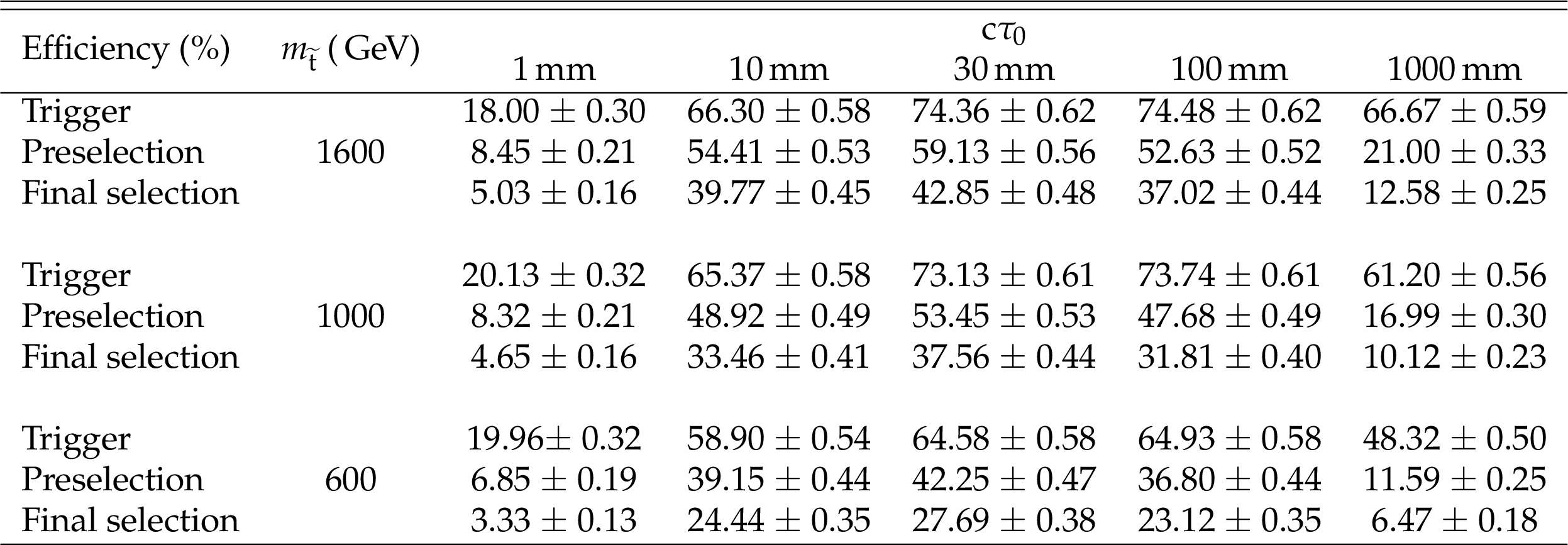
Table 11:
Signal efficiencies (in %) for the $\tilde{\mathrm{t}} \to \mathrm{b} \ell $ model at different proper decay lengths $c\tau _{0}$ and different masses $m_{\mathrm {\tilde{\mathrm{t}}}}$. Selection requirements are cumulative from the first row to the last. Uncertainties are statistical only. |

png pdf |
Table 12:
Signal efficiencies (in %) for the $\tilde{\mathrm{t}} \to \mathrm{d} \ell $ model in 2017 and 2018 at different proper decay lengths $c\tau _{0}$ and different masses $m_{\mathrm {\tilde{\mathrm{t}}}}$. Selection requirements are cumulative from the first row to the last. Uncertainties are statistical only. |
png pdf |
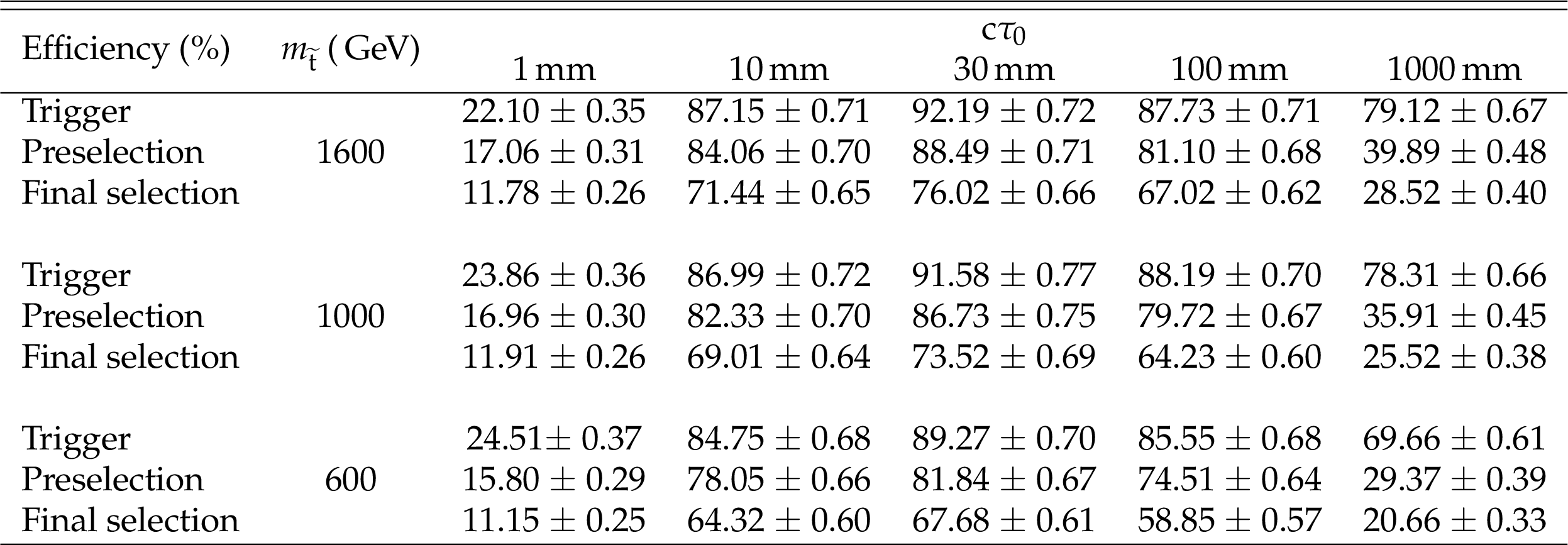
Table 13:
Signal efficiencies (in %) for the $\tilde{\mathrm{t}} \to \mathrm{\bar{d}} \mathrm{\bar{d}} $ model in 2017 and 2018 at different proper decay lengths $c\tau _{0}$ and different masses $m_{\mathrm {\tilde{\mathrm{t}}}}$. Selection requirements are cumulative from the first row to the last. Uncertainties are statistical only. |
| Summary |
| We present a search for long-lived particles decaying to jets, using proton-proton collision data collected with the CMS experiment at a center-of-mass energy of 13 TeV in 2017 and 2018. The results are combined with a previous CMS search for displaced jets search using proton-proton collision data in 2016, accumulating to a total integrated luminosity of 132 fb$^{-1}$ . After all selections, we observe one event in the data collected in 2017 and 2018, which is consistent with the predicted background yield. We set the best current limits on a variety of models with long-lived particles having mean proper decay lengths between 1 mm and 10 m. For a simplified model where pair-produced long-lived neutral particles decay to quark-antiquark pairs, pair production cross sections larger than 0.07 fb are excluded at 95% confidence level for mean proper decay lengths between 2 and 250 mm at high mass ($m_{\mathrm{X}} > $ 500 GeV). For a model where the SM Higgs boson decays to two long-lived scalars and each long-lived scalar decays to a quark-antiquark pair, the branching fractions for the exotic Higgs decay larger than 1% are excluded at 95% confidence level for mean proper decay lengths between 1 mm and 1 m when scalar mass is 40 or 55 GeV. For a supersymmetric (SUSY) model in the general gauge mediation scenario, where the long-lived gluino decays to a gluon and a lightest SUSY particle, gluino masses up to 2450 GeV are excluded at 95% confidence level for mean proper decay lengths between 6 and 550 mm. For another SUSY model in the mini-split scenario, where the long-lived gluino can decay to a quark-antiquark pair and the lightest neutralino, gluino masses up to 2500 GeV are excluded at 95% confidence level for mean proper decay lengths between 7 and 360 mm. An $R$-parity violating (RPV) SUSY model is also tested, where the long-lived gluino can decay to top, bottom, and strange antiquarks, and gluino masses up to 2500 GeV are excluded at 95% confidence level for mean proper decay lengths between 3 and 1000 mm. We also study another RPV SUSY model, where the long-lived top squark can decay to a bottom quark and a charged lepton, and top squark masses up to 1600 GeV are excluded at 95% confidence level for mean proper decay lengths between 5 and 240 mm. For an RPV SUSY model, where the long-lived top squark can decay to a down quark and a charged lepton, top squark masses up to 1600 GeV are excluded at 95% confidence level for mean proper decay lengths between 3 and 360 mm. Finally, for a dynamical-RPV SUSY model, where the long-lived top squark can decay to two down antiquarks, top squark masses up to 1600 GeV are excluded at 95% confidence level for mean proper decay lengths between 2 and 1320 mm. These are the most stringent limits to date on these models. |
| References | ||||
| 1 | N. Arkani-Hamed and S. Dimopoulos | Supersymmetric unification without low energy supersymmetry and signatures for fine-tuning at the LHC | JHEP 06 (2005) 073 | hep-th/0405159 |
| 2 | G. F. Giudice and A. Romanino | Split supersymmetry | NPB 699 (2004) 65 | hep-ph/0406088 |
| 3 | J. L. Hewett, B. Lillie, M. Masip, and T. G. Rizzo | Signatures of long-lived gluinos in split supersymmetry | JHEP 09 (2004) 070 | hep-ph/0408248 |
| 4 | N. Arkani-Hamed, S. Dimopoulos, G. F. Giudice, and A. Romanino | Aspects of split supersymmetry | NPB 709 (2005) 3 | hep-ph/0409232 |
| 5 | P. Gambino, G. F. Giudice, and P. Slavich | Gluino decays in split supersymmetry | NPB 726 (2005) 35 | hep-ph/0506214 |
| 6 | A. Arvanitaki, N. Craig, S. Dimopoulos, and G. Villadoro | Mini-split | JHEP 02 (2013) 126 | 1210.0555 |
| 7 | N. Arkani-Hamed et al. | Simply unnatural supersymmetry | 1212.6971 | |
| 8 | P. Fayet | Supergauge invariant extension of the Higgs mechanism and a model for the electron and its neutrino | NPB 90 (1975) 104 | |
| 9 | G. R. Farrar and P. Fayet | Phenomenology of the production, decay, and detection of new hadronic states associated with supersymmetry | PLB 76 (1978) 575 | |
| 10 | S. Weinberg | Supersymmetry at ordinary energies. 1. masses and conservation laws | PRD 26 (1982) 287 | |
| 11 | L. J. Hall and M. Suzuki | Explicit $ R $-parity breaking in supersymmetric models | NPB 231 (1984) 419 | |
| 12 | R. Barbier et al. | $ R $-parity violating supersymmetry | PR 420 (2005) 1 | hep-ph/0406039 |
| 13 | G. F. Giudice and R. Rattazzi | Theories with gauge mediated supersymmetry breaking | PR 322 (1999) 419 | hep-ph/9801271 |
| 14 | P. Meade, N. Seiberg, and D. Shih | General gauge mediation | Prog. Theor. Phys. Suppl. 177 (2009) 143 | 0801.3278 |
| 15 | M. Buican, P. Meade, N. Seiberg, and D. Shih | Exploring general gauge mediation | JHEP 03 (2009) 016 | 0812.3668 |
| 16 | J. Fan, M. Reece, and J. T. Ruderman | Stealth supersymmetry | JHEP 11 (2011) 012 | 1105.5135 |
| 17 | J. Fan, M. Reece, and J. T. Ruderman | A stealth supersymmetry sampler | JHEP 07 (2012) 196 | 1201.4875 |
| 18 | M. J. Strassler and K. M. Zurek | Echoes of a hidden valley at hadron colliders | PLB 651 (2007) 374 | hep-ph/0604261 |
| 19 | M. J. Strassler and K. M. Zurek | Discovering the Higgs through highly-displaced vertices | PLB 661 (2008) 263 | hep-ph/0605193 |
| 20 | T. Han, Z. Si, K. M. Zurek, and M. J. Strassler | Phenomenology of hidden valleys at hadron colliders | JHEP 07 (2008) 008 | 0712.2041 |
| 21 | D. E. Kaplan, M. A. Luty, and K. M. Zurek | Asymmetric dark matter | PRD 79 (2009) 115016 | 0901.4117 |
| 22 | L. J. Hall, K. Jedamzik, J. March-Russell, and S. M. West | Freeze-in production of FIMP dark matter | JHEP 03 (2010) 080 | 0911.1120 |
| 23 | I.-W. Kim and K. M. Zurek | Flavor and collider signatures of asymmetric dark matter | PRD 89 (2014) 035008 | 1310.2617 |
| 24 | Y. Cui and B. Shuve | Probing baryogenesis with displaced vertices at the LHC | JHEP 02 (2015) 049 | 1409.6729 |
| 25 | R. T. Co, F. D'Eramo, L. J. Hall, and D. Pappadopulo | Freeze-In dark matter with displaced signatures at colliders | JCAP 1512 (2015) 024 | 1506.07532 |
| 26 | L. Calibbi, L. Lopez-Honorez, S. Lowette, and A. Mariotti | Singlet-Doublet dark matter freeze-in: LHC displaced signatures versus cosmology | JHEP 09 (2018) 037 | 1805.04423 |
| 27 | Y. Cui, L. Randall, and B. Shuve | A WIMPy baryogenesis miracle | JHEP 04 (2012) 075 | 1112.2704 |
| 28 | Y. Cui and R. Sundrum | Baryogenesis for weakly interacting massive particles | PRD 87 (2013) 116013 | 1212.2973 |
| 29 | A. Atre, T. Han, S. Pascoli, and B. Zhang | The search for heavy Majorana neutrinos | JHEP 05 (2009) 030 | 0901.3589 |
| 30 | M. Drewes | The phenomenology of right handed neutrinos | Int. J. Mod. Phys. E 22 (2013) 1330019 | 1303.6912 |
| 31 | F. F. Deppisch, P. S. Bhupal Dev, and A. Pilaftsis | Neutrinos and collider physics | New J. Phys. 17 (2015) 075019 | 1502.06541 |
| 32 | Y. Cai, T. Han, T. Li, and R. Ruiz | Lepton Number Violation: Seesaw Models and Their Collider Tests | Front. Phys. 6 (2018) 40 | 1711.02180 |
| 33 | Z. Chacko, H.-S. Goh, and R. Harnik | Natural electroweak breaking from a mirror symmetry | PRL 96 (2006) 231802 | hep-ph/0506256 |
| 34 | H. Cai, H.-C. Cheng, and J. Terning | A quirky little Higgs model | JHEP 05 (2009) 045 | 0812.0843 |
| 35 | N. Craig, S. Knapen, and P. Longhi | Neutral Naturalness from Orbifold Higgs Models | PRL 114 (2015) 061803 | 1410.6808 |
| 36 | N. Craig, A. Katz, M. Strassler, and R. Sundrum | Naturalness in the dark at the LHC | JHEP 07 (2015) 105 | 1501.05310 |
| 37 | D. Curtin and C. B. Verhaaren | Discovering uncolored naturalness in exotic Higgs decays | JHEP 12 (2015) 072 | 1506.06141 |
| 38 | CMS Collaboration | The CMS experiment at the CERN LHC | JINST 3 (2008) S08004 | CMS-00-001 |
| 39 | CMS Collaboration | Search for long-lived particles decaying into displaced jets in proton-proton collisions at $ \sqrt{s}= $ 13 TeV | PRD 99 (2019) 032011 | CMS-EXO-18-007 1811.07991 |
| 40 | ATLAS Collaboration | Search for long-lived, massive particles in events with displaced vertices and missing transverse momentum in $ \sqrt{s} = 13 TeV pp $ collisions with the ATLAS detector | PRD 97 (2018) 052012 | 1710.04901 |
| 41 | ATLAS Collaboration | Search for long-lived particles produced in $ pp $ collisions at $ \sqrt{s}= $ 13 TeV that decay into displaced hadronic jets in the ATLAS muon spectrometer | PRD 99 (2019) 052005 | 1811.07370 |
| 42 | ATLAS Collaboration | Search for long-lived neutral particles in $ pp $ collisions at $ \sqrt{s} = $ 13 TeV that decay into displaced hadronic jets in the ATLAS calorimeter | EPJC 79 (2019) 481 | 1902.03094 |
| 43 | ATLAS Collaboration | Search for long-lived, massive particles in events with a displaced vertex and a muon with large impact parameter in $ pp $ collisions at $ \sqrt{s} = $ 13 TeV with the ATLAS detector | 2003.11956 | |
| 44 | ATLAS Collaboration | Search for long-lived neutral particles produced in $ pp $ collisions at $ \sqrt{s} = $ 13 TeV decaying into displaced hadronic jets in the ATLAS inner detector and muon spectrometer | PRD 101 (2020) 052013 | 1911.12575 |
| 45 | CMS Collaboration | Search for new long-lived particles at $ \sqrt{s} = $ 13 TeV | PLB 780 (2018) 432 | CMS-EXO-16-003 1711.09120 |
| 46 | CMS Collaboration | Search for long-lived particles with displaced vertices in multijet events in proton-proton collisions at $ \sqrt{s}= $ 13 TeV | PRD 98 (2018) 092011 | CMS-EXO-17-018 1808.03078 |
| 47 | CMS Collaboration | Search for long-lived particles using nonprompt jets and missing transverse momentum with proton-proton collisions at $ \sqrt{s} = $ 13 TeV | PLB 797 (2019) 134876 | CMS-EXO-19-001 1906.06441 |
| 48 | CMS Collaboration | The CMS trigger system | JINST 12 (2017) P01020 | CMS-TRG-12-001 1609.02366 |
| 49 | M. Cacciari, G. P. Salam, and G. Soyez | The anti-$ {k_{\mathrm{T}}} $ jet clustering algorithm | JHEP 04 (2008) 063 | 0802.1189 |
| 50 | M. Cacciari, G. P. Salam, and G. Soyez | FastJet user manual | EPJC 72 (2012) 1896 | 1111.6097 |
| 51 | CMS Collaboration | Jet energy scale and resolution in the CMS experiment in pp collisions at 8 TeV | JINST 12 (2017) P02014 | CMS-JME-13-004 1607.03663 |
| 52 | CMS Collaboration | Technical proposal for the Phase-II upgrade of the CMS detector | CMS-PAS-TDR-15-002 | CMS-PAS-TDR-15-002 |
| 53 | J. Alwall et al. | The automated computation of tree-level and next-to-leading order differential cross sections, and their matching to parton shower simulations | JHEP 07 (2014) 079 | 1405.0301 |
| 54 | T. Sjostrand et al. | An introduction to PYTHIA 8.2 | CPC 191 (2015) 159 | 1410.3012 |
| 55 | J. Alwall et al. | Comparative study of various algorithms for the merging of parton showers and matrix elements in hadronic collisions | EPJC 53 (2008) 473 | 0706.2569 |
| 56 | CMS Collaboration | Extraction and validation of a new set of CMS PYTHIA8 tunes from underlying-event measurements | EPJC 80 (2020) 4 | CMS-GEN-17-001 1903.12179 |
| 57 | NNPDF Collaboration | Parton distributions from high-precision collider data | EPJC 77 (2017) 663 | 1706.00428 |
| 58 | LHC Higgs Cross Section Working Group Collaboration | Handbook of LHC Higgs cross sections: 4. Deciphering the nature of the Higgs sector | 1610.07922 | |
| 59 | G. Burdman, Z. Chacko, H.-S. Goh, and R. Harnik | Folded supersymmetry and the LEP paradox | JHEP 02 (2007) 009 | hep-ph/0609152 |
| 60 | P. Nason | A New method for combining NLO QCD with shower Monte Carlo algorithms | JHEP 11 (2004) 040 | hep-ph/0409146 |
| 61 | S. Frixione, P. Nason, and C. Oleari | Matching NLO QCD computations with parton shower simulations: the POWHEG method | JHEP 11 (2007) 070 | 0709.2092 |
| 62 | S. Alioli, P. Nason, C. Oleari, and E. Re | A general framework for implementing NLO calculations in shower Monte Carlo programs: the POWHEG BOX | JHEP 06 (2010) 043 | 1002.2581 |
| 63 | E. Bagnaschi, G. Degrassi, P. Slavich, and A. Vicini | Higgs production via gluon fusion in the POWHEG approach in the SM and in the MSSM | JHEP 02 (2012) 088 | 1111.2854 |
| 64 | Z. Liu and B. Tweedie | The fate of long-lived superparticles with hadronic decays after LHC Run 1 | JHEP 06 (2015) 042 | 1503.05923 |
| 65 | C. Csaki, Y. Grossman, and B. Heidenreich | Minimal flavor violation supersymmetry: a natural theory for $ R $-parity violation | PRD 85 (2012) 095009 | 1111.1239 |
| 66 | P. W. Graham, D. E. Kaplan, S. Rajendran, and P. Saraswat | Displaced supersymmetry | JHEP 07 (2012) 149 | 1204.6038 |
| 67 | C. Csaki, E. Kuflik, and T. Volansky | Dynamical $ R $-parity violation | PRL 112 (2014) 131801 | 1309.5957 |
| 68 | C. Csaki, E. Kuflik, O. Slone, and T. Volansky | Models of dynamical $ R $-parity violation | JHEP 06 (2015) 045 | 1502.03096 |
| 69 | C. Csaki et al. | Phenomenology of a long-lived LSP with $ R $-parity violation | JHEP 08 (2015) 016 | 1505.00784 |
| 70 | G. R. Farrar and P. Fayet | Bounds on $ R $-hadron production from calorimetry experiments | PLB 79 (1978) 442 | |
| 71 | M. Fairbairn et al. | Stable massive particles at colliders | PR 438 (2007) 1 | hep-ph/0611040 |
| 72 | R. Mackeprang and A. Rizzi | Interactions of coloured heavy stable particles in matter | EPJC 50 (2007) 353 | hep-ph/0612161 |
| 73 | GEANT4 Collaboration | GEANT4--a simulation toolkit | NIMA 506 (2003) 250 | |
| 74 | CMS Collaboration | Description and performance of track and primary-vertex reconstruction with the CMS tracker | JINST 9 (2014) P10009 | CMS-TRK-11-001 1405.6569 |
| 75 | R. Fruhwirth, W. Waltenberger, and P. Vanlaer | Adaptive vertex fitting | JPG 34 (2007) N343 | |
| 76 | CMS Collaboration | Precision measurement of the structure of the CMS inner tracking system using nuclear interactions | JINST 13 (2018) P10034 | CMS-TRK-17-001 1807.03289 |
| 77 | CMS Collaboration | CMS technical design report for the pixel detector upgrade | CERN-LHCC-2012-016, CMS-TDR-011 | |
| 78 | S. C. Johnson | Hierarchical clustering schemes | Psychometrika 32 (1967) 241 | |
| 79 | Y. Freund and R. E. Schapire | Experiments with a new boosting algorithm | in Proceedings of the Thirteenth International Conference on International Conference on Machine Learning, ICML'96, p. 148 Morgan Kaufmann Publishers Inc., San Francisco, CA, USA | |
| 80 | J. Friedman, T. Hastie, and R. Tibshirani | Additive logistic regression: a statistical view of boosting (with discussion and a rejoinder by the authors) | Ann. Statist. 28 (2000) 337 | |
| 81 | J. H. Friedman | Greedy function approximation: A gradient boosting machine. | Ann. Statist. 29 (2001) 1189 | |
| 82 | H. Voss, A. Hocker, J. Stelzer, and F. Tegenfeldt | TMVA, the toolkit for multivariate data analysis with ROOT | in XIth International Workshop on Advanced Computing and Analysis Techniques in Physics Research (ACAT), p. 40 2007 [PoS(ACAT)040] | physics/0703039 |
| 83 | F. Pedregosa et al. | Scikit-learn: Machine learning in Python | J. Mach. Learn. Res. 12 (2011) 2825 | |
| 84 | CMS Collaboration | CMS luminosity measurement for the 2017 data-taking period at $ \sqrt{s} = $ 13 TeV | ||
| 85 | CMS Collaboration | CMS luminosity measurement for the 2018 data-taking period at $ \sqrt{s} = $ 13 TeV | ||
| 86 | S. Dulat et al. | New parton distribution functions from a global analysis of quantum chromodynamics | PRD 93 (2016) 033006 | 1506.07443 |
| 87 | L. A. Harland-Lang, A. D. Martin, P. Motylinski, and R. S. Thorne | Parton distributions in the LHC era: MMHT 2014 PDFs | EPJC 75 (2015) 204 | 1412.3989 |
| 88 | J. Butterworth et al. | PDF4LHC recommendations for LHC Run II | JPG 43 (2016) 023001 | 1510.03865 |
| 89 | A. Buckley et al. | LHAPDF6: parton density access in the LHC precision era | EPJC 75 (2015) 132 | 1412.7420 |
| 90 | T. Junk | Confidence level computation for combining searches with small statistics | NIMA 434 (1999) 435 | hep-ex/9902006 |
| 91 | A. L. Read | Presentation of search results: The CLs technique | JPG 28 (2002) 2693 | |
| 92 | G. Cowan, K. Cranmer, E. Gross, and O. Vitells | Asymptotic formulae for likelihood-based tests of new physics | EPJC 71 (2011) 1554 | 1007.1727 |
| 93 | The ATLAS Collaboration, The CMS Collaboration, The LHC Higgs Combination Group | Procedure for the LHC Higgs boson search combination in Summer 2011 | CMS-NOTE-2011-005 | |
| 94 | W. Beenakker, R. Hopker, M. Spira, and P. M. Zerwas | Squark and gluino production at hadron colliders | NPB 492 (1997) 51 | hep-ph/9610490 |
| 95 | A. Kulesza and L. Motyka | Threshold resummation for squark-antisquark and gluino-pair production at the LHC | PRL 102 (2009) 111802 | 0807.2405 |
| 96 | A. Kulesza and L. Motyka | Soft gluon resummation for the production of gluino-gluino and squark-antisquark pairs at the LHC | PRD 80 (2009) 095004 | 0905.4749 |
| 97 | W. Beenakker et al. | Squark and gluino hadroproduction | Int. J. Mod. Phys. A 26 (2011) 2637 | 1105.1110 |
| 98 | C. Borschensky et al. | Squark and gluino production cross sections in pp collisions at $ \sqrt{s} = $ 13, 14, 33 and 100 TeV | EPJC 74 (2014) 3174 | 1407.5066 |
| 99 | W. Beenakker et al. | NNLL-fast: predictions for coloured supersymmetric particle production at the LHC with threshold and Coulomb resummation | JHEP 12 (2016) 133 | 1607.07741 |
|
|
Compact Muon Solenoid LHC, CERN |
|

|

|

|

|

|