

Compact Muon Solenoid
LHC, CERN
| CMS-PAS-EXO-19-009 | ||
| A search for new physics in central exclusive production using the missing mass technique with the CMS-TOTEM precision proton spectrometer | ||
| CMS Collaboration | ||
| March 2022 | ||
| Abstract: A generic search is presented for associated production of a Z boson or a photon with an additional unspecified massive particle X in proton-tagged events from pp collisions at $\sqrt{s} = $ 13 TeV, recorded in 2017 by the CMS detector and the CMS-TOTEM precision proton spectrometer. The so-called missing mass spectrum is analysed in the 600-1600 GeV range and a fit is performed to search for possible deviations from the background expectation. Model-independent upper limits on the visible production cross section of pp $\rightarrow$ pp $+$ Z/$\gamma$ $+$ X are set, in the absence of significant resonant deviations in data with respect to the background predictions. | ||
|
Links:
CDS record (PDF) ;
CADI line (restricted) ;
These preliminary results are superseded in this paper, Submitted to EPJC. The superseded preliminary plots can be found here. |
||
| Figures | |
png pdf |
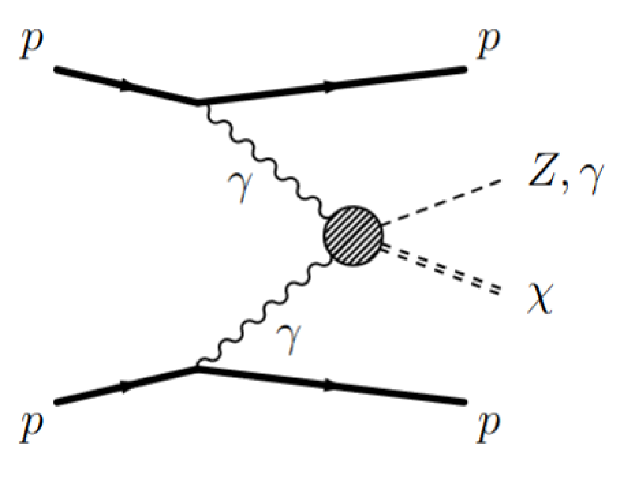
Figure 1:
Schematic diagram of two-photon production of a Z boson or photon with an additional, unknown particle $\chi $ giving rise to a missing mass $m_{\rm miss} = m_\chi $. The production mechanism does not have to proceed through photon exchange. Other colourless exchange mechanisms (e.g. double pomeron) are also allowed. However, at such a high energy scale, electroweak processes become dominant as QCD-based colourless exchanges are expected to be suppressed. |

png pdf |
Figure 2:
Schematic drawing of the CT-PPS detectors used in this analysis. The left (right) arm in this plot is located on the positive (negative) side of the $z$ axis in the CMS coordinate system. |
png pdf |
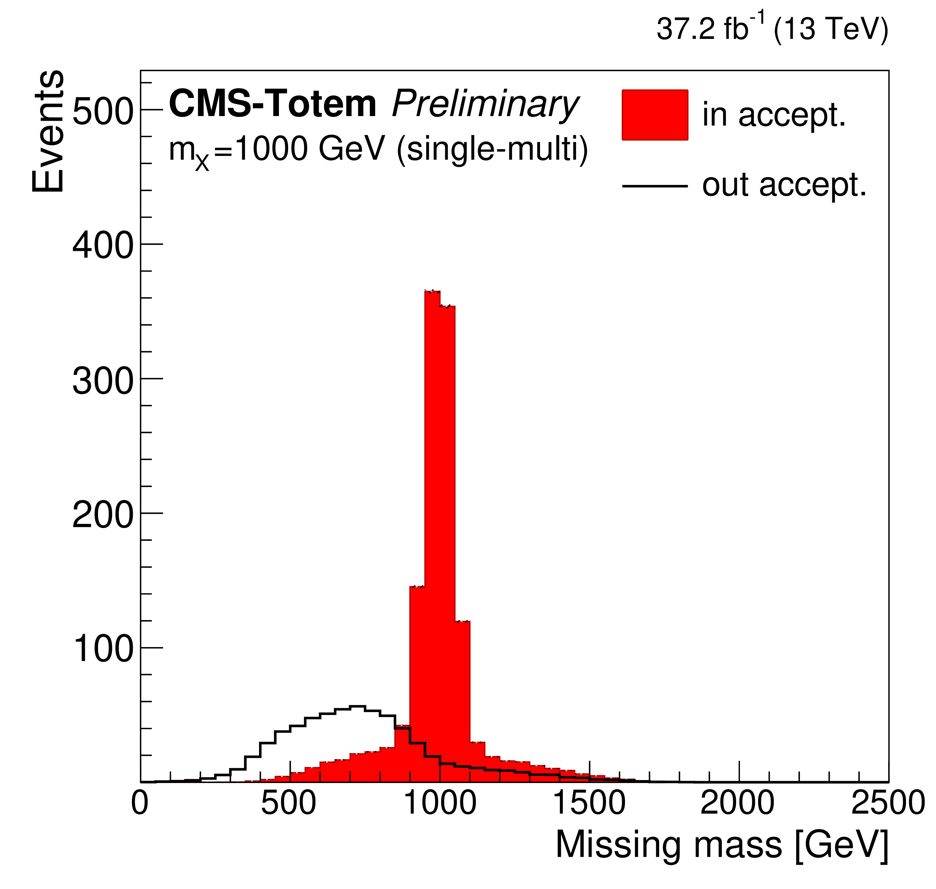
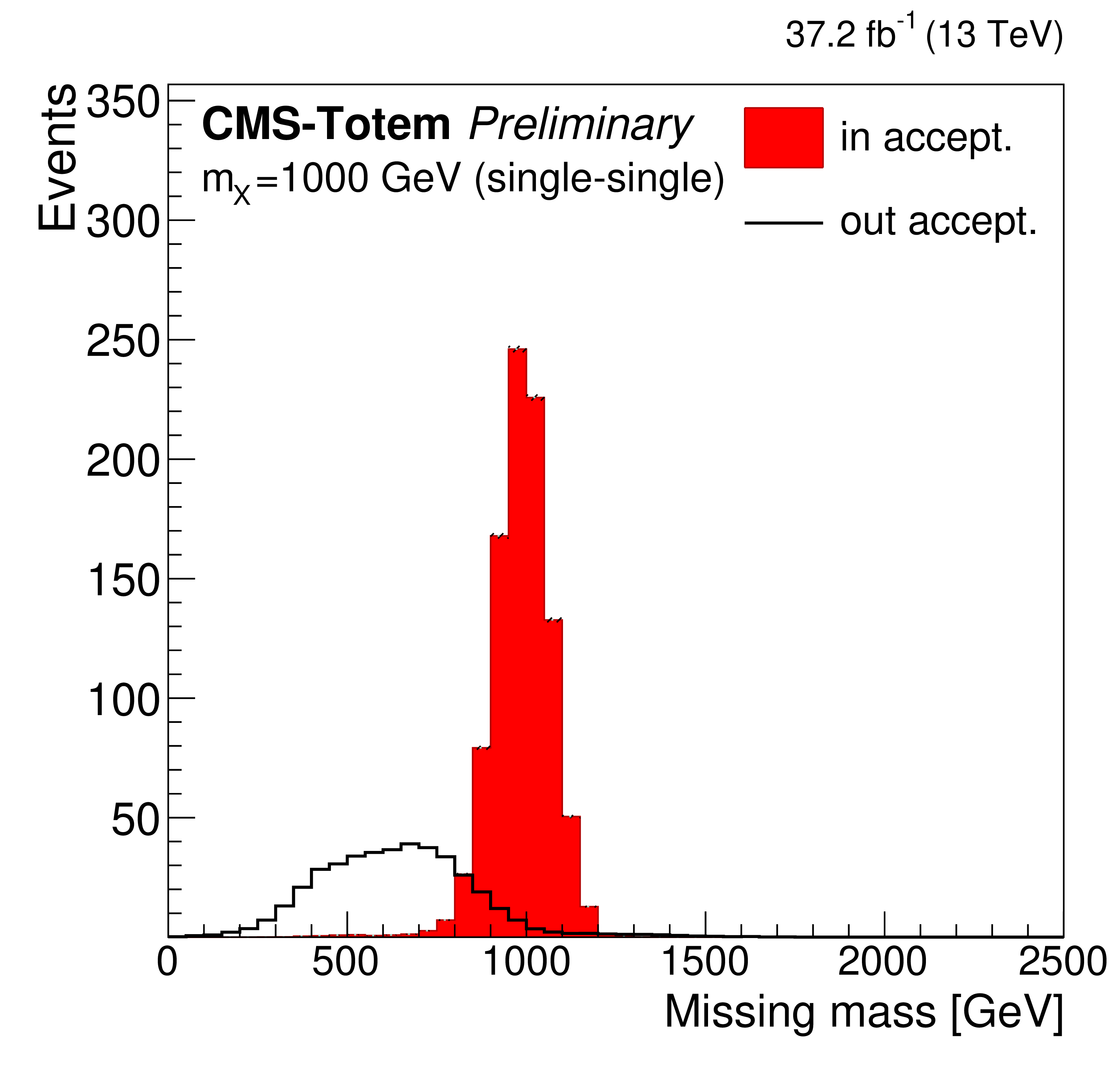
Figure 3:
Comparison of the missing mass shapes for the simulated signal events within the fiducial region and those outside it, after the mixing of pileup protons and selection of the protons, for a generated $m_X$ mass of 1000 GeV. From left to right the distributions are shown for the different proton reconstruction categories: multi(+)-multi(-), multi(+)-single(-), single(+)-multi(-) and single(+)-single(-). |
png pdf |
Figure 3-a:
Comparison of the missing mass shapes for the simulated signal events within the fiducial region and those outside it, after the mixing of pileup protons and selection of the protons, for a generated $m_X$ mass of 1000 GeV. From left to right the distributions are shown for the different proton reconstruction categories: multi(+)-multi(-), multi(+)-single(-), single(+)-multi(-) and single(+)-single(-). |
png pdf |
Figure 3-b:
Comparison of the missing mass shapes for the simulated signal events within the fiducial region and those outside it, after the mixing of pileup protons and selection of the protons, for a generated $m_X$ mass of 1000 GeV. From left to right the distributions are shown for the different proton reconstruction categories: multi(+)-multi(-), multi(+)-single(-), single(+)-multi(-) and single(+)-single(-). |
png pdf |
Figure 3-c:
Comparison of the missing mass shapes for the simulated signal events within the fiducial region and those outside it, after the mixing of pileup protons and selection of the protons, for a generated $m_X$ mass of 1000 GeV. From left to right the distributions are shown for the different proton reconstruction categories: multi(+)-multi(-), multi(+)-single(-), single(+)-multi(-) and single(+)-single(-). |
png pdf |
Figure 3-d:
Comparison of the missing mass shapes for the simulated signal events within the fiducial region and those outside it, after the mixing of pileup protons and selection of the protons, for a generated $m_X$ mass of 1000 GeV. From left to right the distributions are shown for the different proton reconstruction categories: multi(+)-multi(-), multi(+)-single(-), single(+)-multi(-) and single(+)-single(-). |
png pdf |
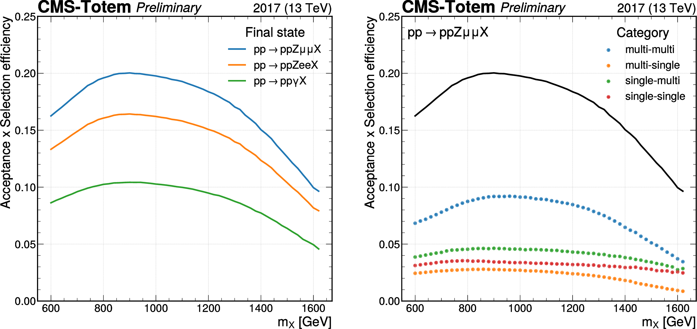
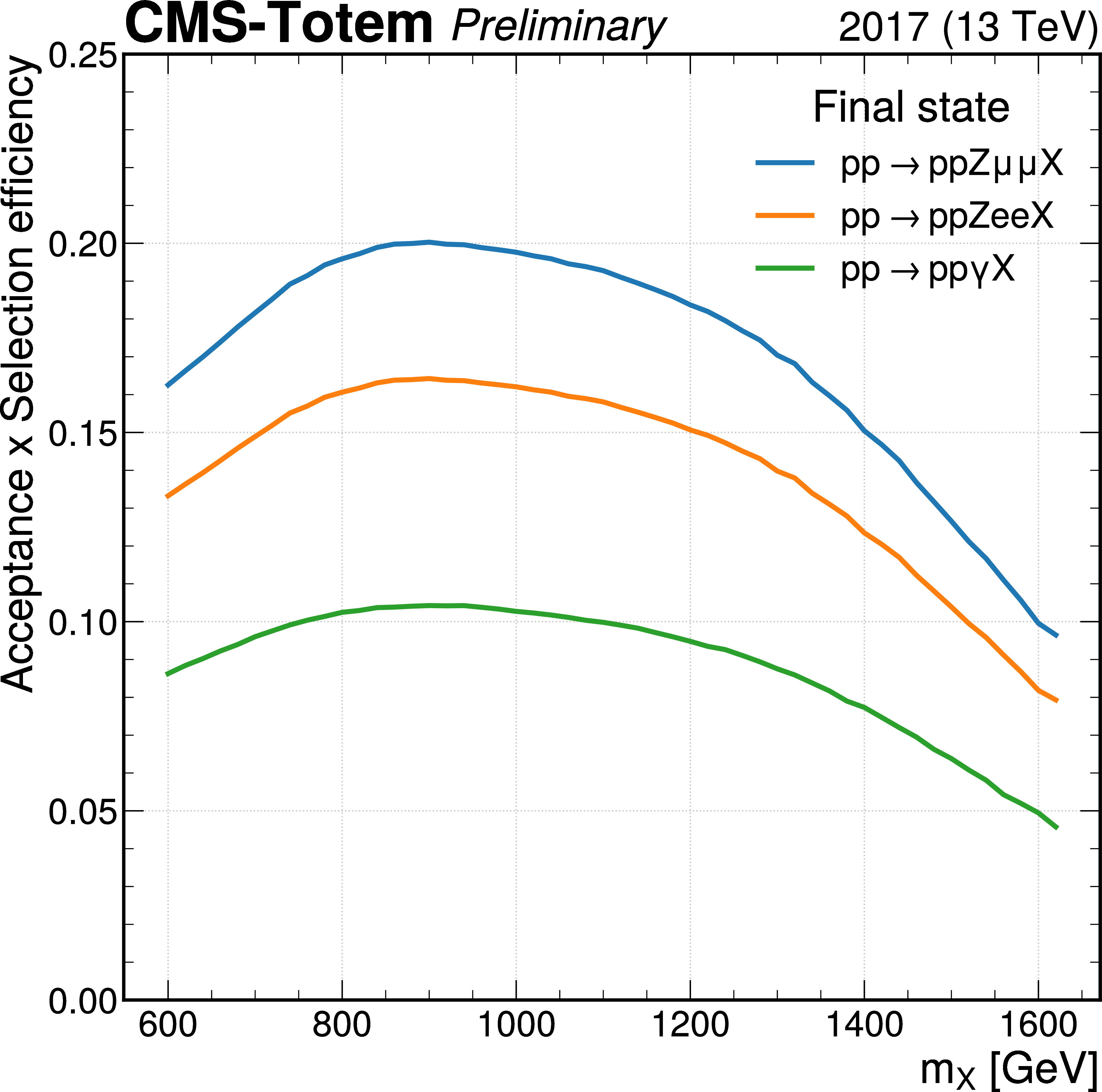
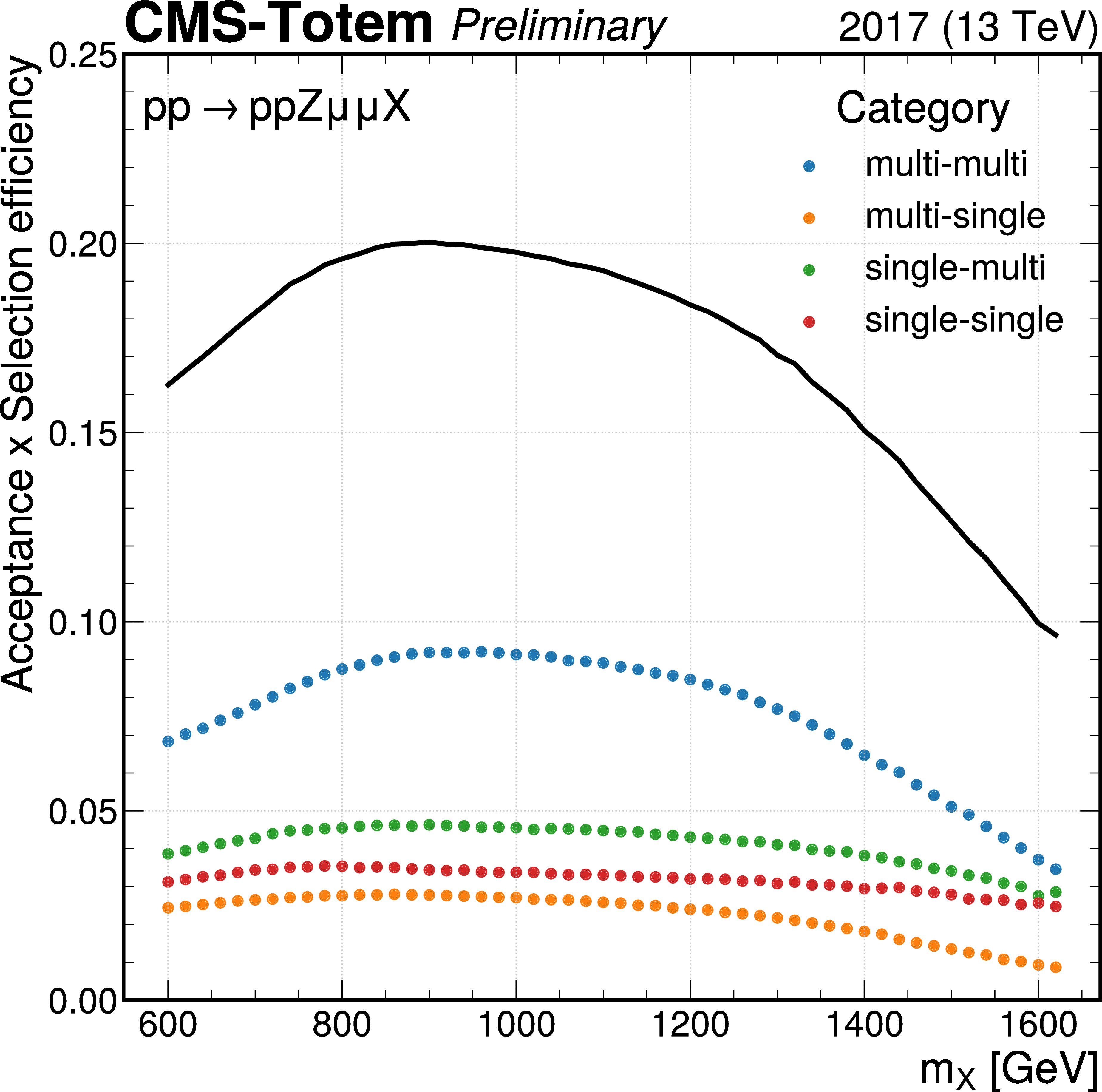
Figure 4:
Product of the acceptance times the combined reconstruction and identification efficiency, as a function of $m_X$, for events generated inside the fiducial volume defined in Tab.1. The curve shown on the left displays the different final states, while the one on the right shows the contributions from the different proton-reconstruction categories to the Z $ \rightarrow \mu \mu $ analysis. The definition of the fiducial region and signal model used to estimate the acceptance is provided in the text. |
png pdf |
Figure 4-a:
Product of the acceptance times the combined reconstruction and identification efficiency, as a function of $m_X$, for events generated inside the fiducial volume defined in Tab.1. The curve shown on the left displays the different final states, while the one on the right shows the contributions from the different proton-reconstruction categories to the Z $ \rightarrow \mu \mu $ analysis. The definition of the fiducial region and signal model used to estimate the acceptance is provided in the text. |
png pdf |
Figure 4-b:
Product of the acceptance times the combined reconstruction and identification efficiency, as a function of $m_X$, for events generated inside the fiducial volume defined in Tab.1. The curve shown on the left displays the different final states, while the one on the right shows the contributions from the different proton-reconstruction categories to the Z $ \rightarrow \mu \mu $ analysis. The definition of the fiducial region and signal model used to estimate the acceptance is provided in the text. |
png pdf |
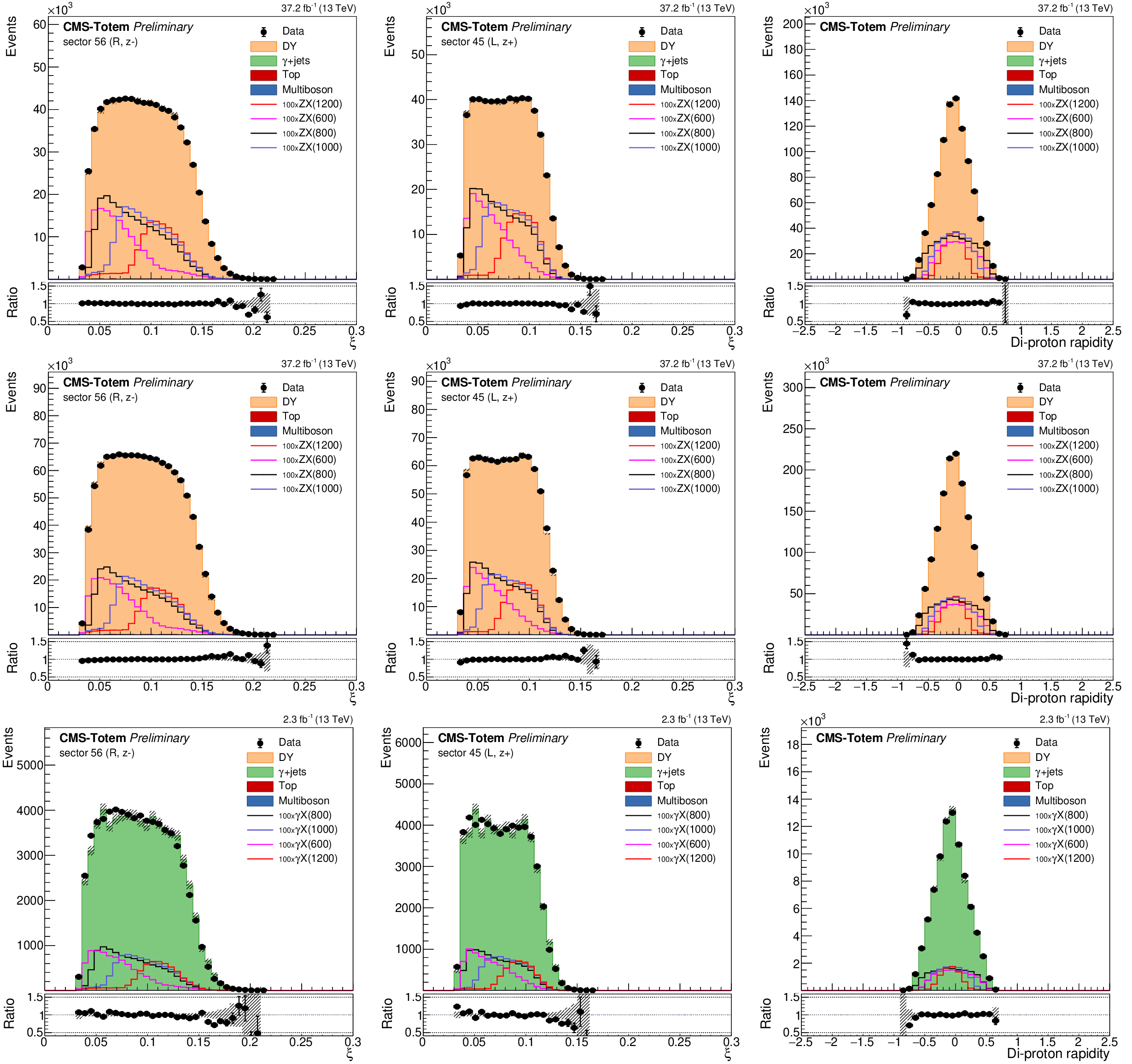
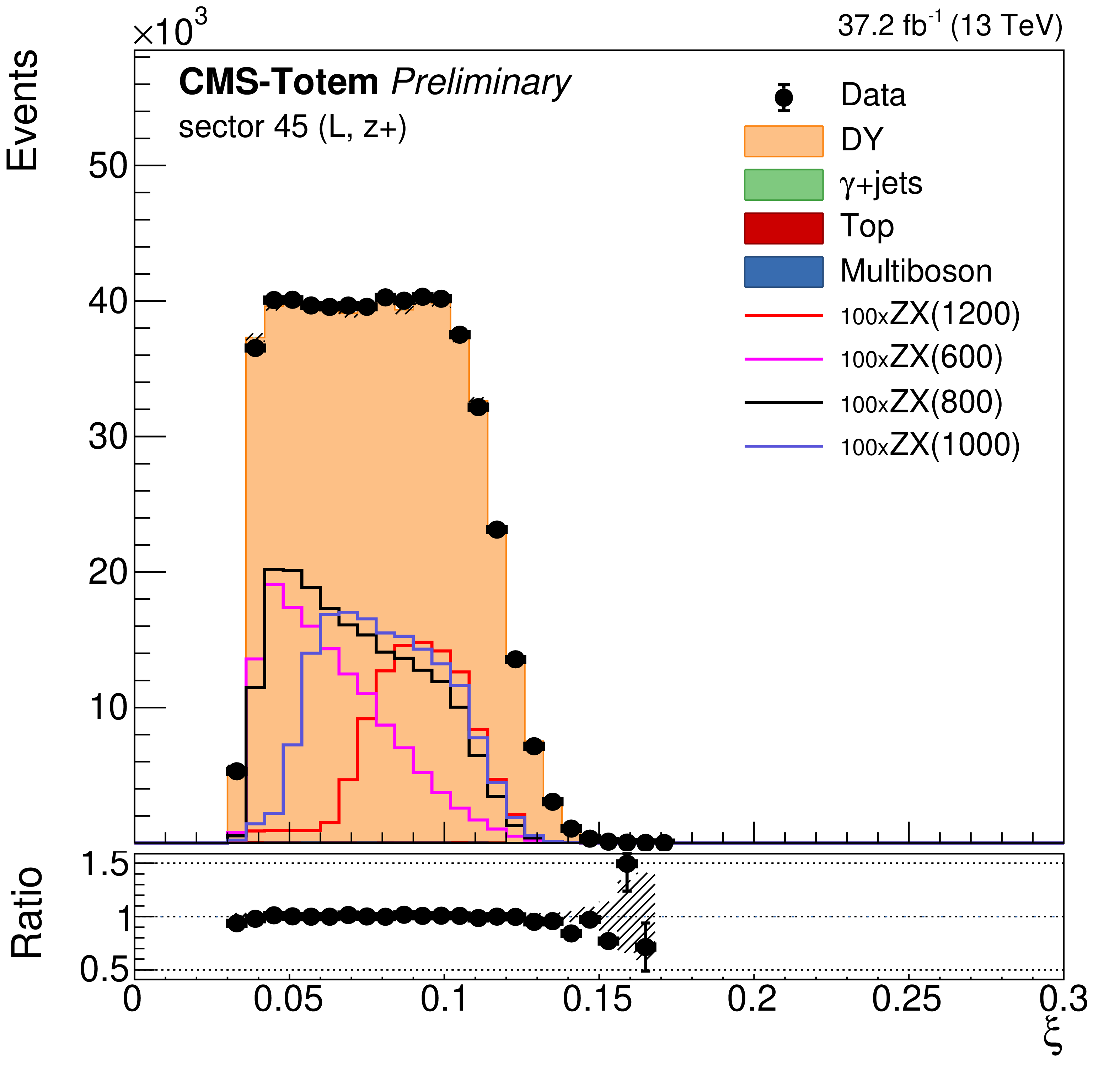
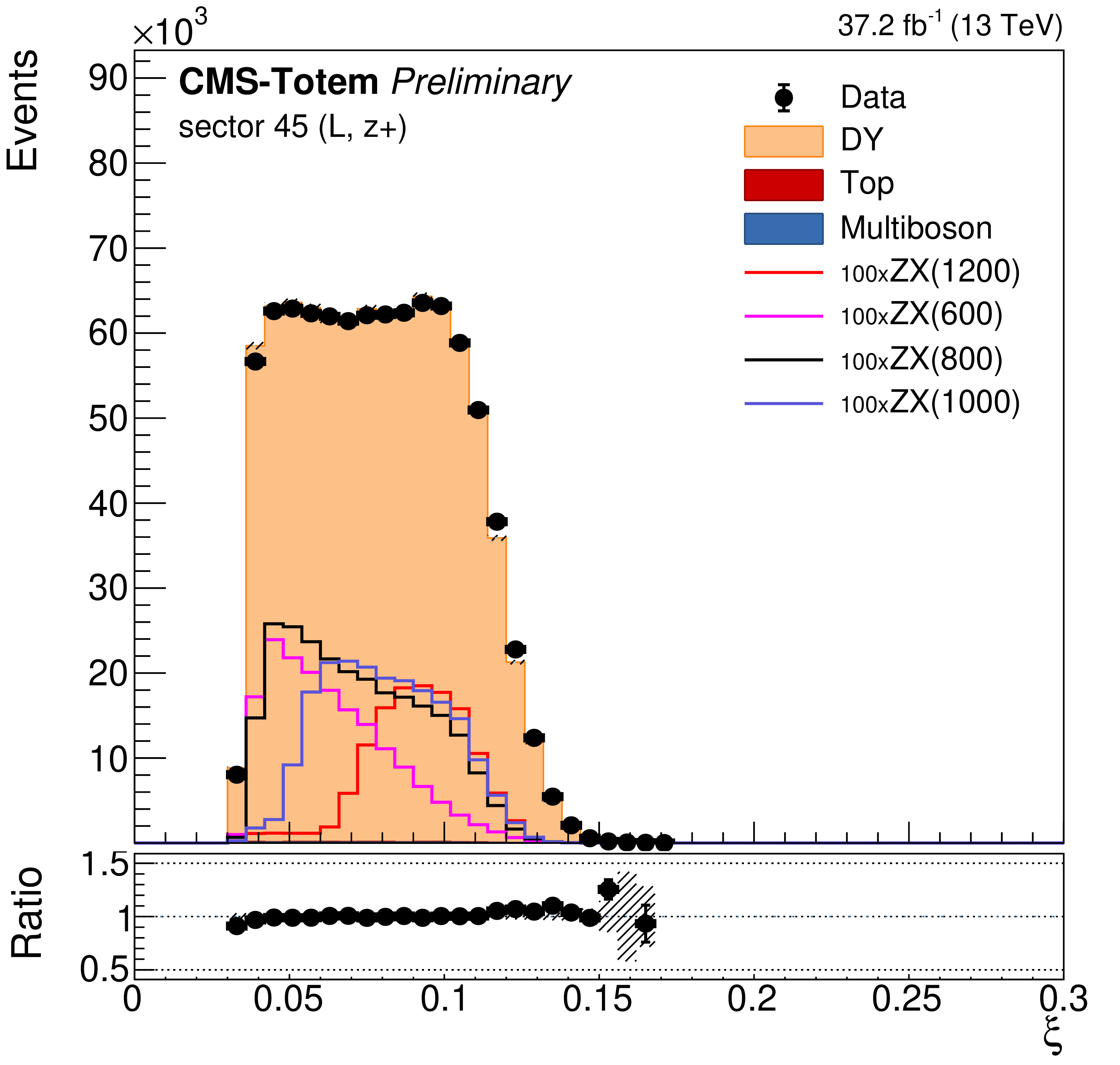
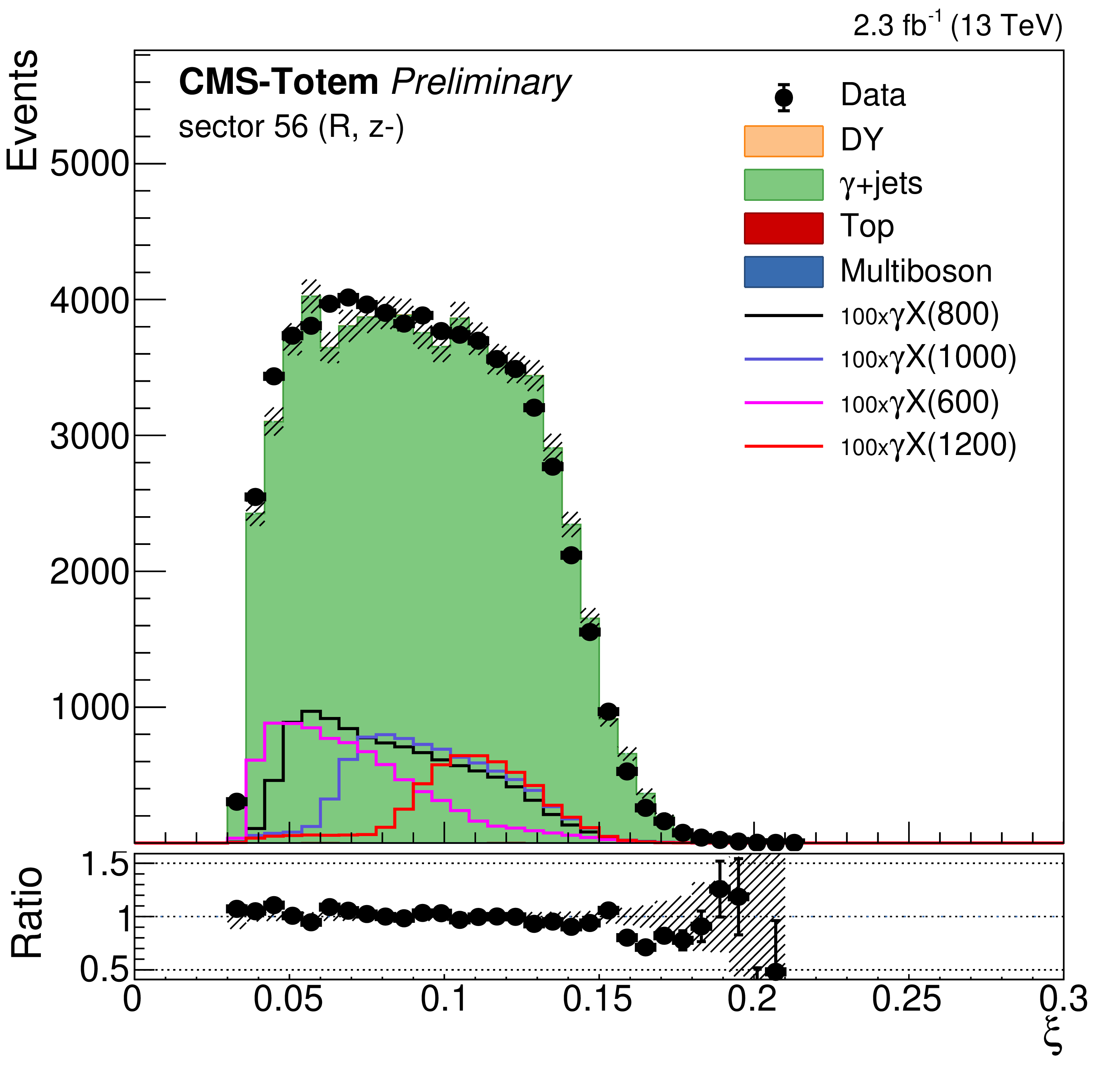
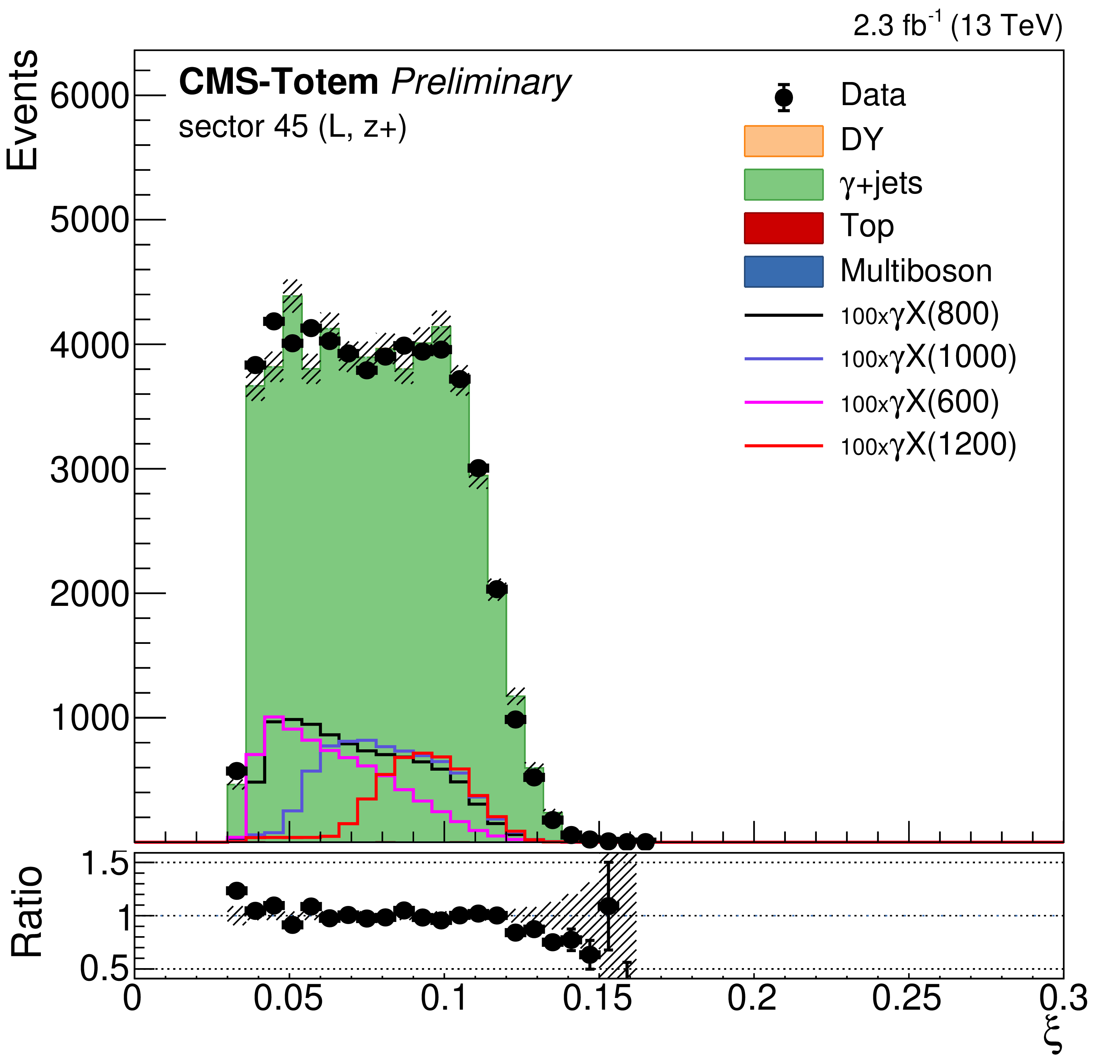
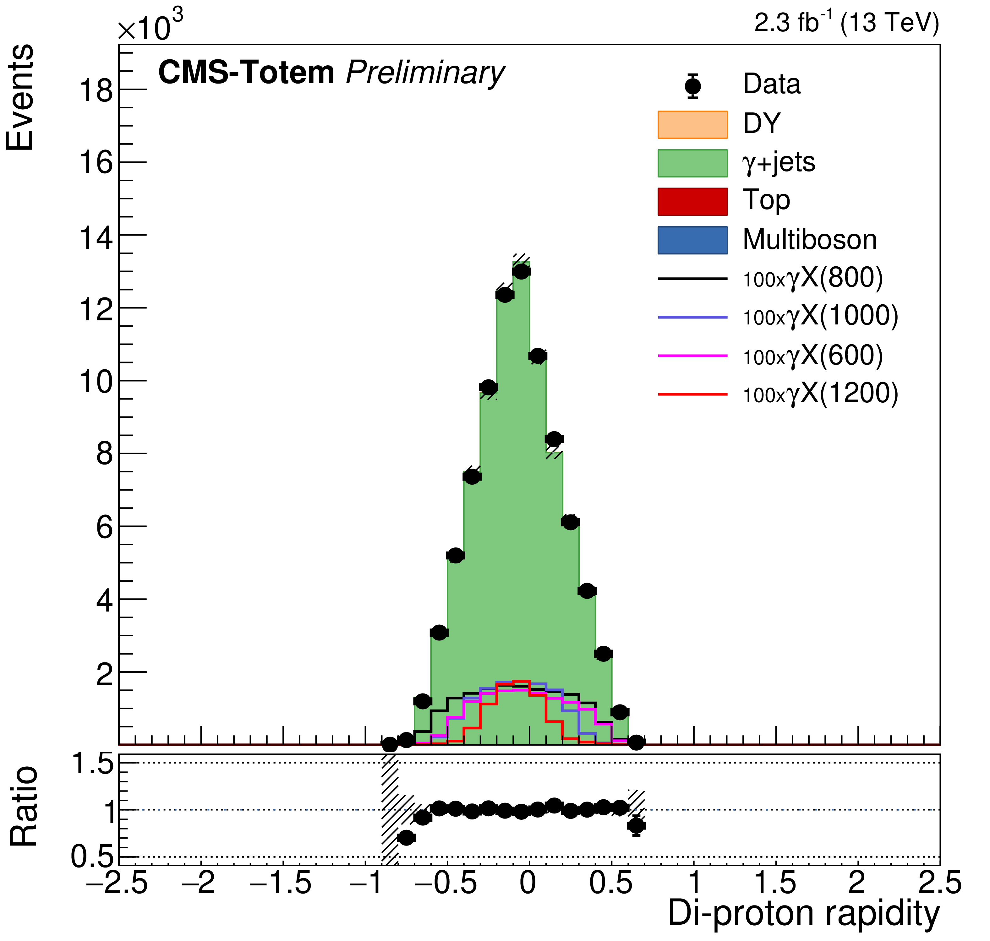
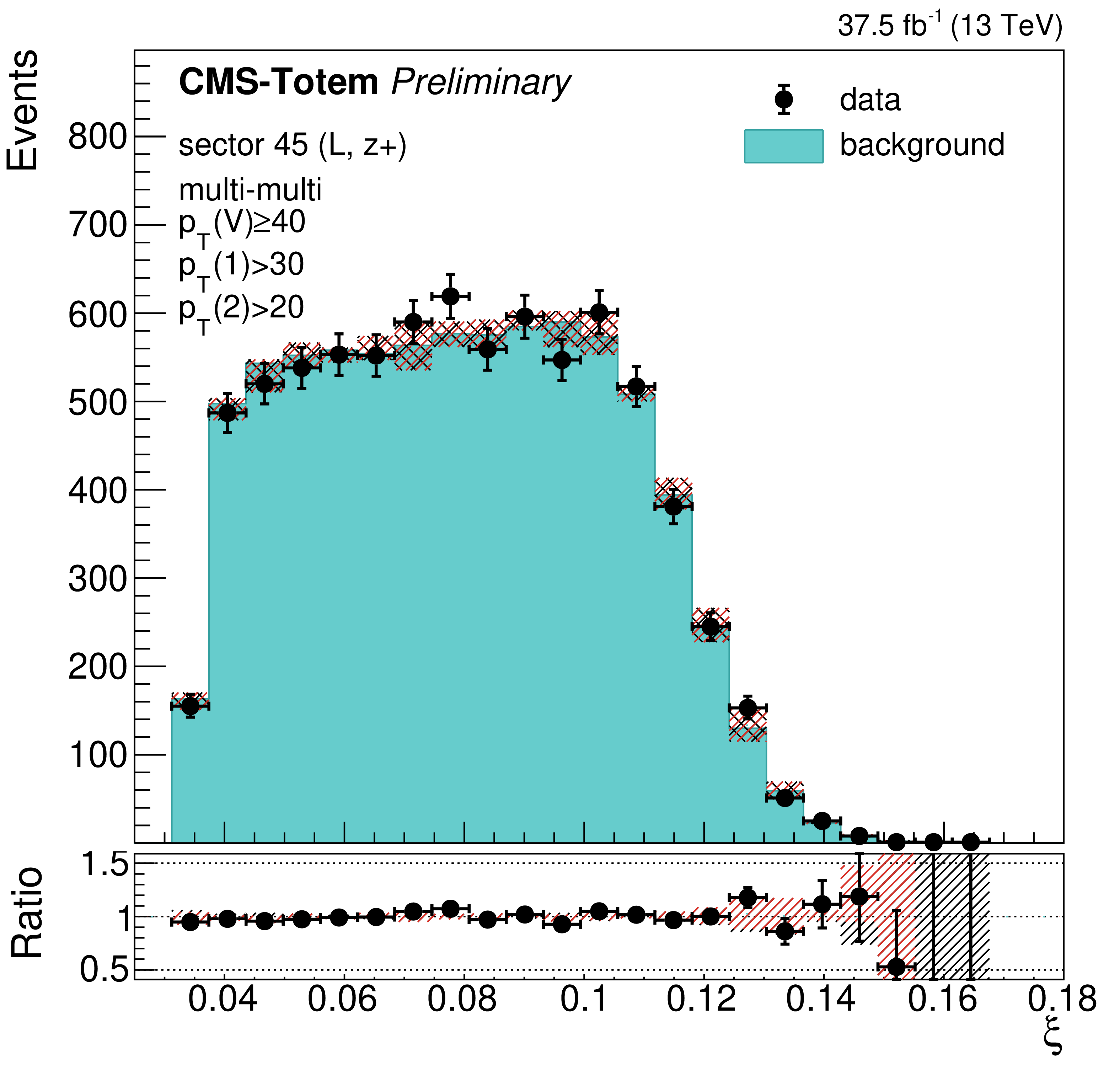
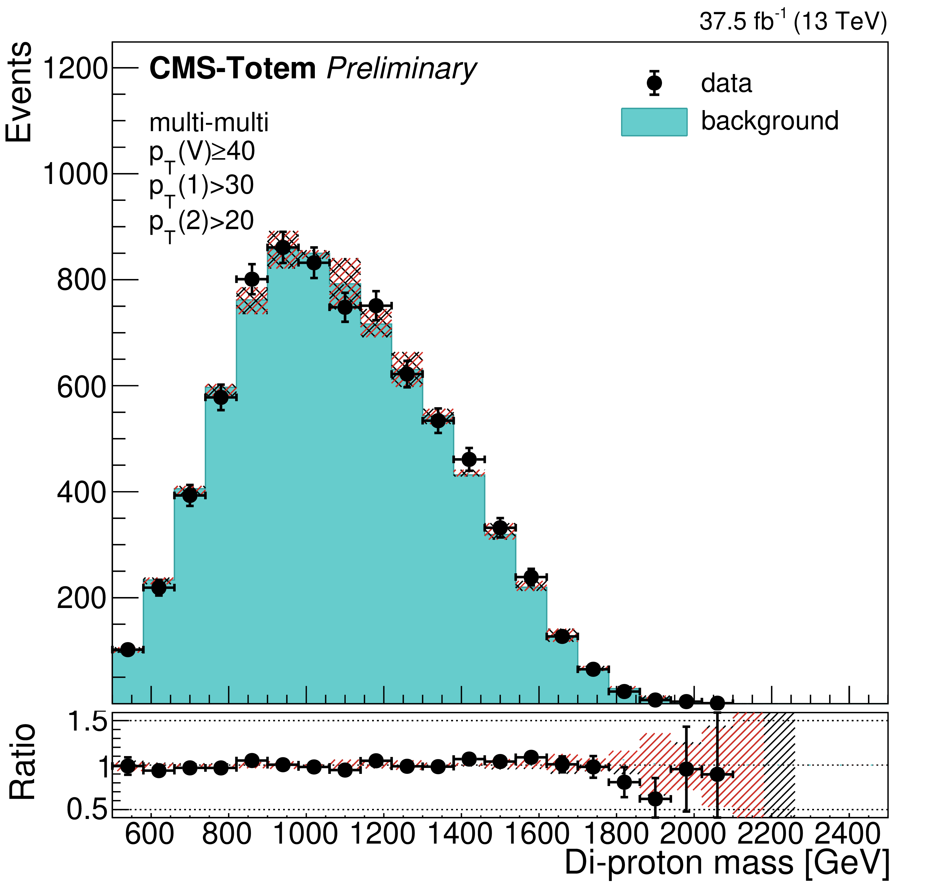
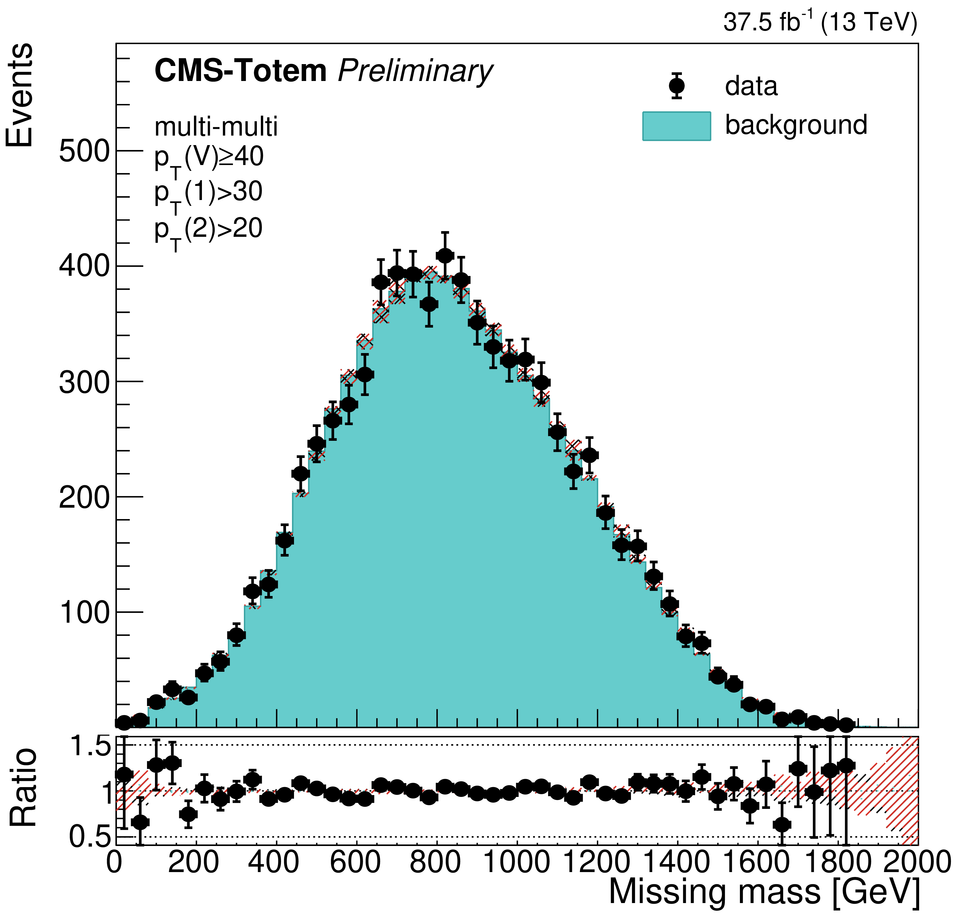
Figure 5:
Modeling of the reconstructed proton $\xi $ in the negative arm (left), positive arm (middle), and the corresponding di-proton rapidity (right) from the proton mixing procedure, using events selected in MC simulation, compared to data. From top to bottom the ee, $\mu \mu $, and photon final states are shown. The ee and $\mu \mu $ events are displayed without Z boson ${p_{\mathrm {T}}}$ requirement. For illustration the simulated signal distributions are superimposed for various choices of $m_X$, normalised to a generated fiducial cross section of 100 pb. |

png pdf |
Figure 5-a:
Modeling of the reconstructed proton $\xi $ in the negative arm (left), positive arm (middle), and the corresponding di-proton rapidity (right) from the proton mixing procedure, using events selected in MC simulation, compared to data. From top to bottom the ee, $\mu \mu $, and photon final states are shown. The ee and $\mu \mu $ events are displayed without Z boson ${p_{\mathrm {T}}}$ requirement. For illustration the simulated signal distributions are superimposed for various choices of $m_X$, normalised to a generated fiducial cross section of 100 pb. |
png pdf |
Figure 5-b:
Modeling of the reconstructed proton $\xi $ in the negative arm (left), positive arm (middle), and the corresponding di-proton rapidity (right) from the proton mixing procedure, using events selected in MC simulation, compared to data. From top to bottom the ee, $\mu \mu $, and photon final states are shown. The ee and $\mu \mu $ events are displayed without Z boson ${p_{\mathrm {T}}}$ requirement. For illustration the simulated signal distributions are superimposed for various choices of $m_X$, normalised to a generated fiducial cross section of 100 pb. |

png pdf |
Figure 5-c:
Modeling of the reconstructed proton $\xi $ in the negative arm (left), positive arm (middle), and the corresponding di-proton rapidity (right) from the proton mixing procedure, using events selected in MC simulation, compared to data. From top to bottom the ee, $\mu \mu $, and photon final states are shown. The ee and $\mu \mu $ events are displayed without Z boson ${p_{\mathrm {T}}}$ requirement. For illustration the simulated signal distributions are superimposed for various choices of $m_X$, normalised to a generated fiducial cross section of 100 pb. |

png pdf |
Figure 5-d:
Modeling of the reconstructed proton $\xi $ in the negative arm (left), positive arm (middle), and the corresponding di-proton rapidity (right) from the proton mixing procedure, using events selected in MC simulation, compared to data. From top to bottom the ee, $\mu \mu $, and photon final states are shown. The ee and $\mu \mu $ events are displayed without Z boson ${p_{\mathrm {T}}}$ requirement. For illustration the simulated signal distributions are superimposed for various choices of $m_X$, normalised to a generated fiducial cross section of 100 pb. |
png pdf |
Figure 5-e:
Modeling of the reconstructed proton $\xi $ in the negative arm (left), positive arm (middle), and the corresponding di-proton rapidity (right) from the proton mixing procedure, using events selected in MC simulation, compared to data. From top to bottom the ee, $\mu \mu $, and photon final states are shown. The ee and $\mu \mu $ events are displayed without Z boson ${p_{\mathrm {T}}}$ requirement. For illustration the simulated signal distributions are superimposed for various choices of $m_X$, normalised to a generated fiducial cross section of 100 pb. |

png pdf |
Figure 5-f:
Modeling of the reconstructed proton $\xi $ in the negative arm (left), positive arm (middle), and the corresponding di-proton rapidity (right) from the proton mixing procedure, using events selected in MC simulation, compared to data. From top to bottom the ee, $\mu \mu $, and photon final states are shown. The ee and $\mu \mu $ events are displayed without Z boson ${p_{\mathrm {T}}}$ requirement. For illustration the simulated signal distributions are superimposed for various choices of $m_X$, normalised to a generated fiducial cross section of 100 pb. |
png pdf |
Figure 5-g:
Modeling of the reconstructed proton $\xi $ in the negative arm (left), positive arm (middle), and the corresponding di-proton rapidity (right) from the proton mixing procedure, using events selected in MC simulation, compared to data. From top to bottom the ee, $\mu \mu $, and photon final states are shown. The ee and $\mu \mu $ events are displayed without Z boson ${p_{\mathrm {T}}}$ requirement. For illustration the simulated signal distributions are superimposed for various choices of $m_X$, normalised to a generated fiducial cross section of 100 pb. |
png pdf |
Figure 5-h:
Modeling of the reconstructed proton $\xi $ in the negative arm (left), positive arm (middle), and the corresponding di-proton rapidity (right) from the proton mixing procedure, using events selected in MC simulation, compared to data. From top to bottom the ee, $\mu \mu $, and photon final states are shown. The ee and $\mu \mu $ events are displayed without Z boson ${p_{\mathrm {T}}}$ requirement. For illustration the simulated signal distributions are superimposed for various choices of $m_X$, normalised to a generated fiducial cross section of 100 pb. |
png pdf |
Figure 5-i:
Modeling of the reconstructed proton $\xi $ in the negative arm (left), positive arm (middle), and the corresponding di-proton rapidity (right) from the proton mixing procedure, using events selected in MC simulation, compared to data. From top to bottom the ee, $\mu \mu $, and photon final states are shown. The ee and $\mu \mu $ events are displayed without Z boson ${p_{\mathrm {T}}}$ requirement. For illustration the simulated signal distributions are superimposed for various choices of $m_X$, normalised to a generated fiducial cross section of 100 pb. |
png pdf |
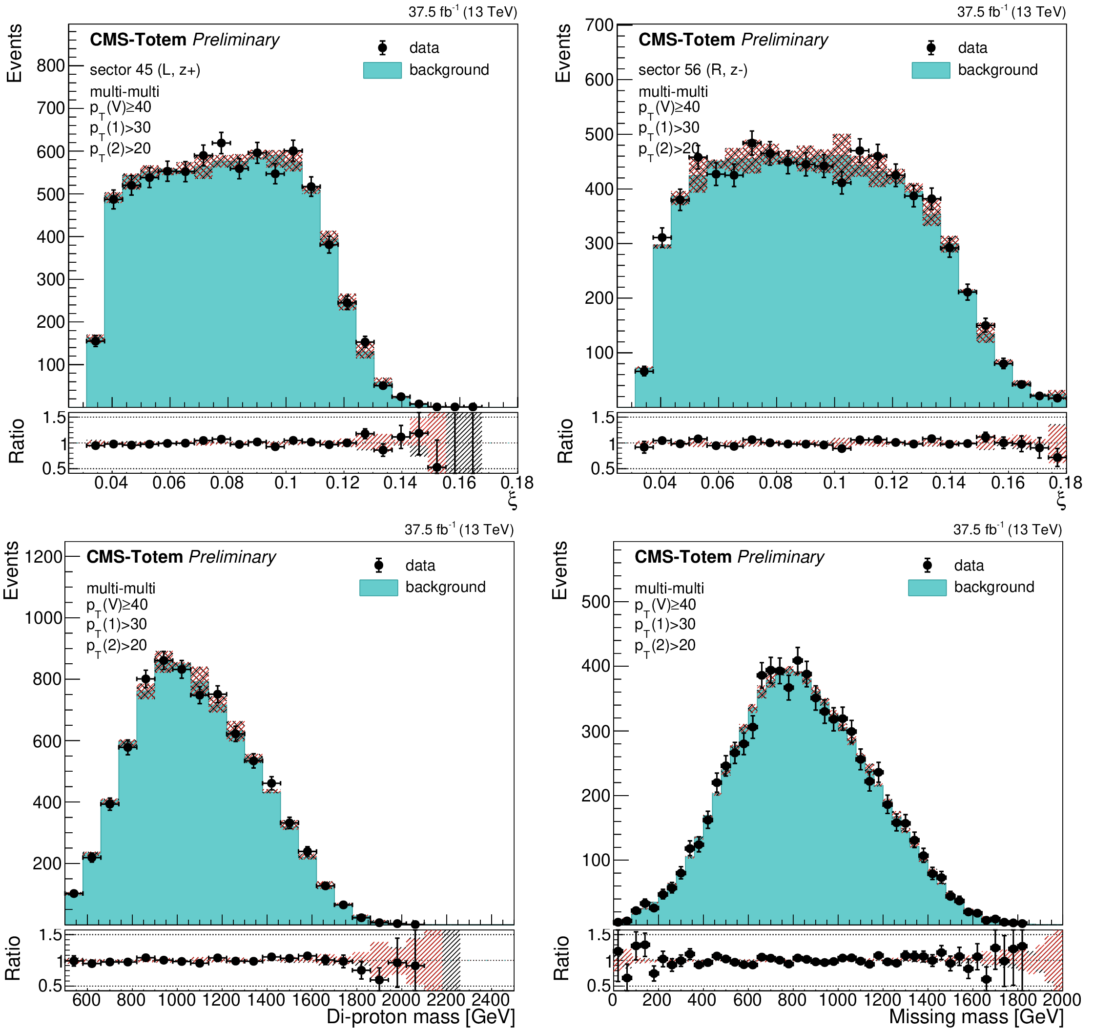
Figure 6:
Validation of the background modeling method, using the e$\mu $ control sample. Selected e$\mu $ events are mixed with protons from Z $ \rightarrow \mu \mu $ events with $ {p_{\mathrm {T}}} (\mathrm{Z}) < $ 10 GeV to simulate the combinatorial background shape, while the data points are unaltered e$\mu $ events. The proton $\xi $ distributions for both CT-PPS arms (top), those of the di-proton invariant mass (bottom left), and of ${m_{\rm miss}}$ (bottom right) are shown. The uncertainty band on the background prediction represents the contribution from the limited statistics and the alternative mixing approaches described in the text. |
png pdf |
Figure 6-a:
Validation of the background modeling method, using the e$\mu $ control sample. Selected e$\mu $ events are mixed with protons from Z $ \rightarrow \mu \mu $ events with $ {p_{\mathrm {T}}} (\mathrm{Z}) < $ 10 GeV to simulate the combinatorial background shape, while the data points are unaltered e$\mu $ events. The proton $\xi $ distributions for both CT-PPS arms (top), those of the di-proton invariant mass (bottom left), and of ${m_{\rm miss}}$ (bottom right) are shown. The uncertainty band on the background prediction represents the contribution from the limited statistics and the alternative mixing approaches described in the text. |

png pdf |
Figure 6-b:
Validation of the background modeling method, using the e$\mu $ control sample. Selected e$\mu $ events are mixed with protons from Z $ \rightarrow \mu \mu $ events with $ {p_{\mathrm {T}}} (\mathrm{Z}) < $ 10 GeV to simulate the combinatorial background shape, while the data points are unaltered e$\mu $ events. The proton $\xi $ distributions for both CT-PPS arms (top), those of the di-proton invariant mass (bottom left), and of ${m_{\rm miss}}$ (bottom right) are shown. The uncertainty band on the background prediction represents the contribution from the limited statistics and the alternative mixing approaches described in the text. |
png pdf |
Figure 6-c:
Validation of the background modeling method, using the e$\mu $ control sample. Selected e$\mu $ events are mixed with protons from Z $ \rightarrow \mu \mu $ events with $ {p_{\mathrm {T}}} (\mathrm{Z}) < $ 10 GeV to simulate the combinatorial background shape, while the data points are unaltered e$\mu $ events. The proton $\xi $ distributions for both CT-PPS arms (top), those of the di-proton invariant mass (bottom left), and of ${m_{\rm miss}}$ (bottom right) are shown. The uncertainty band on the background prediction represents the contribution from the limited statistics and the alternative mixing approaches described in the text. |
png pdf |
Figure 6-d:
Validation of the background modeling method, using the e$\mu $ control sample. Selected e$\mu $ events are mixed with protons from Z $ \rightarrow \mu \mu $ events with $ {p_{\mathrm {T}}} (\mathrm{Z}) < $ 10 GeV to simulate the combinatorial background shape, while the data points are unaltered e$\mu $ events. The proton $\xi $ distributions for both CT-PPS arms (top), those of the di-proton invariant mass (bottom left), and of ${m_{\rm miss}}$ (bottom right) are shown. The uncertainty band on the background prediction represents the contribution from the limited statistics and the alternative mixing approaches described in the text. |

png pdf |
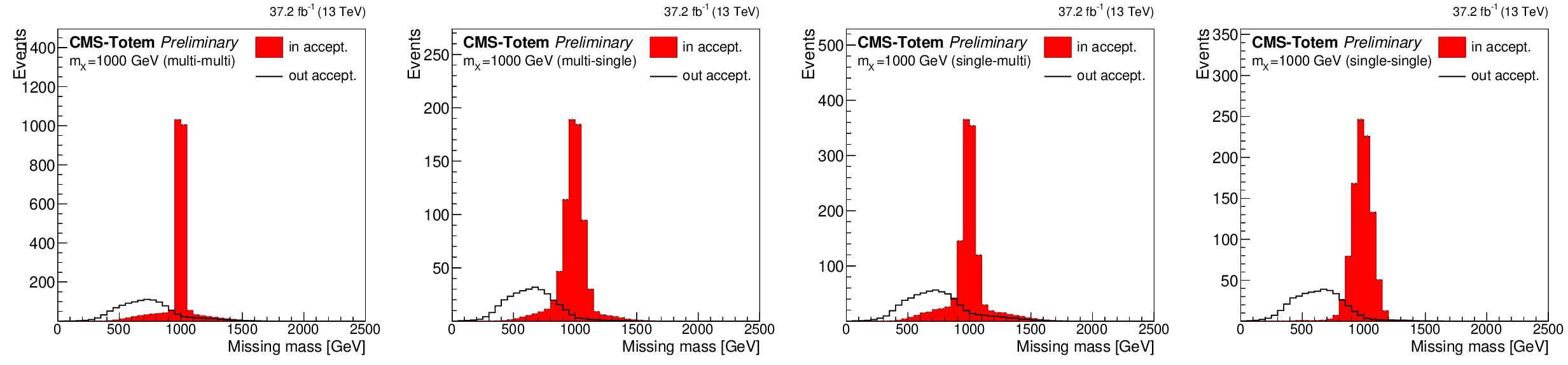
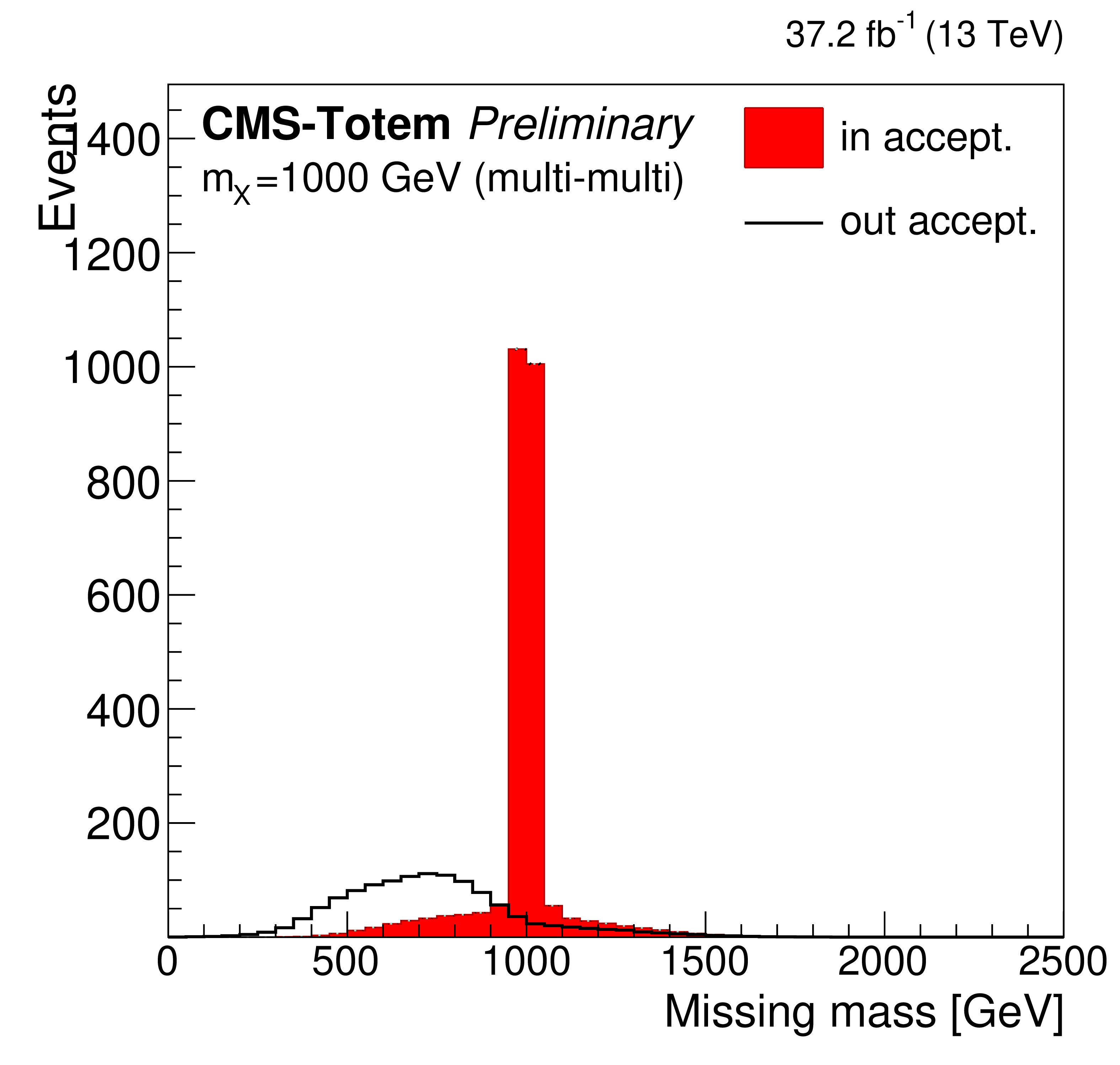
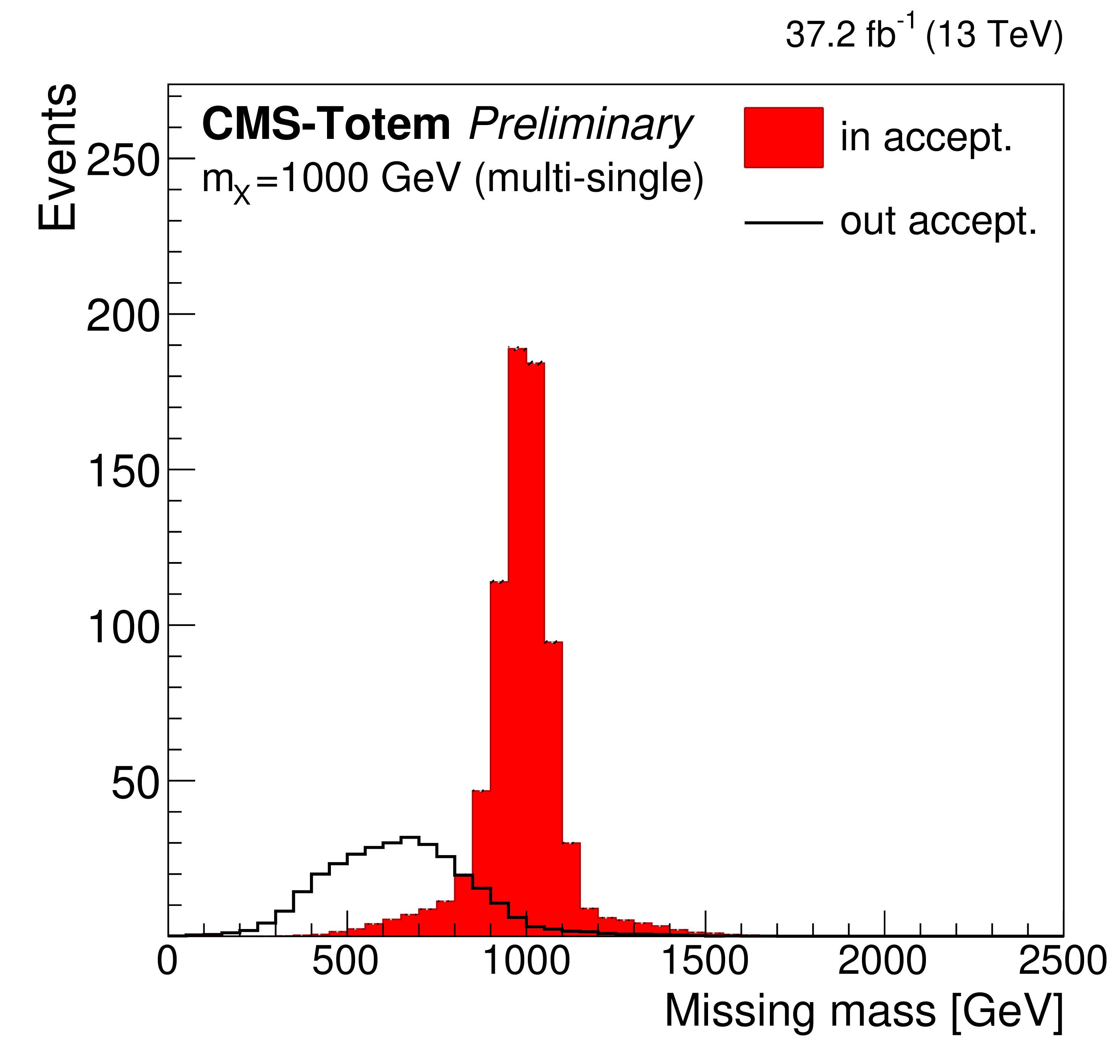
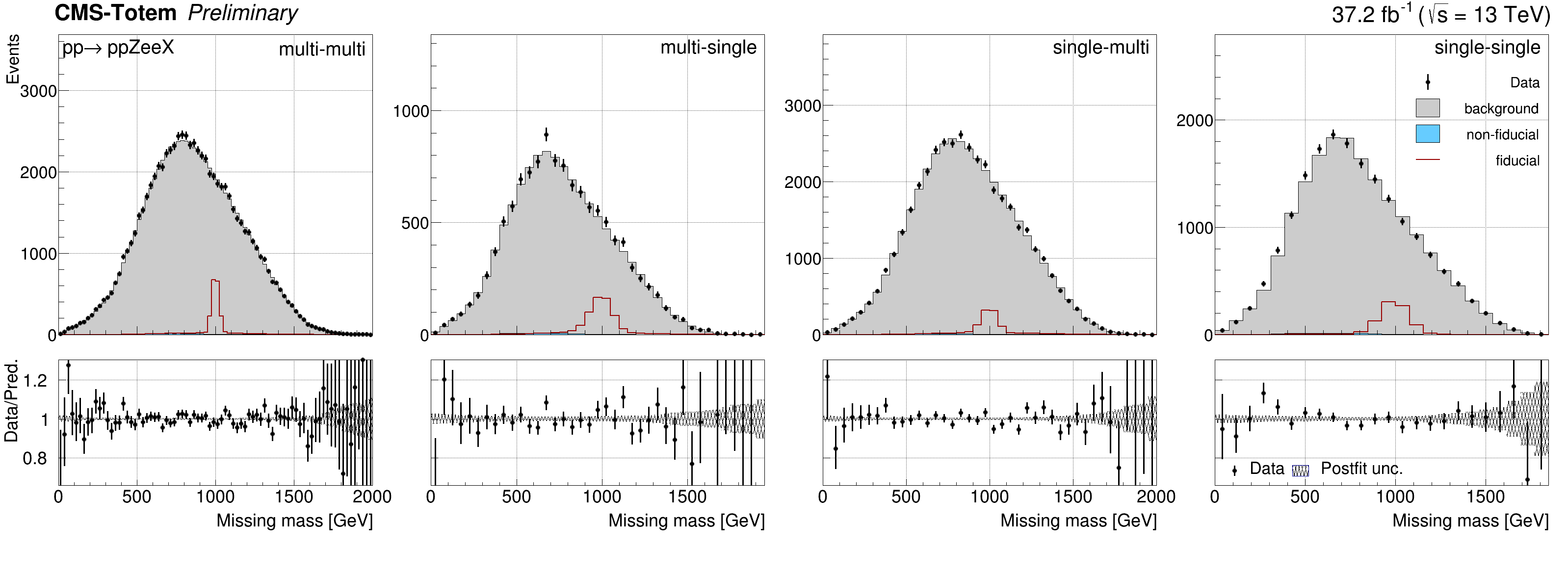
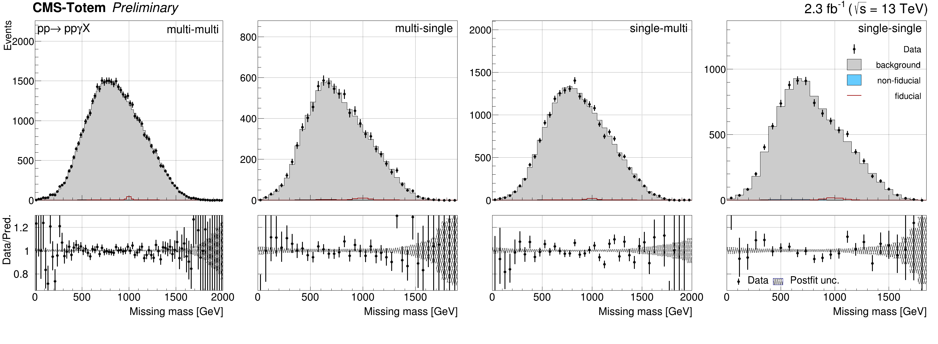
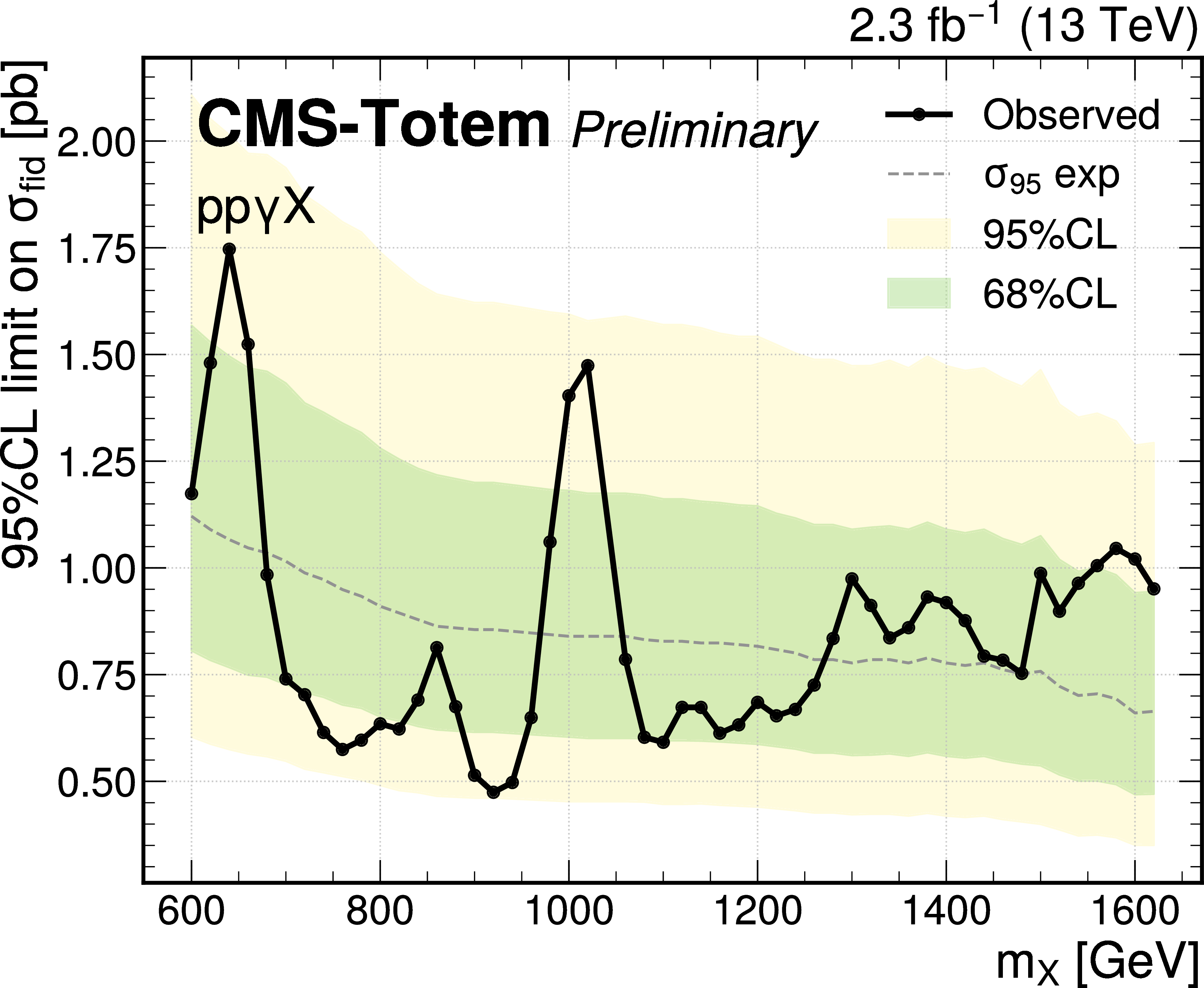
Figure 7:
${m_{\rm miss}}$ distributions in the Z $ \rightarrow \mu \mu $ (top), Z $ \rightarrow $ ee (middle), and $\gamma $ (bottom) final states. From the left to the right the distributions are shown in categories making use of protons reconstructed with the multi-multi, multi-single, single-multi and single-single methods, respectively. The background distributions are shown after the fit. The expectations for a signal with $m_X = $ 1000 GeV are superimposed, where in each channel the fiducial production cross section is normalised to 1 pb. |
png |
Figure 7-a:
${m_{\rm miss}}$ distributions in the Z $ \rightarrow \mu \mu $ (top), Z $ \rightarrow $ ee (middle), and $\gamma $ (bottom) final states. From the left to the right the distributions are shown in categories making use of protons reconstructed with the multi-multi, multi-single, single-multi and single-single methods, respectively. The background distributions are shown after the fit. The expectations for a signal with $m_X = $ 1000 GeV are superimposed, where in each channel the fiducial production cross section is normalised to 1 pb. |

png |
Figure 7-b:
${m_{\rm miss}}$ distributions in the Z $ \rightarrow \mu \mu $ (top), Z $ \rightarrow $ ee (middle), and $\gamma $ (bottom) final states. From the left to the right the distributions are shown in categories making use of protons reconstructed with the multi-multi, multi-single, single-multi and single-single methods, respectively. The background distributions are shown after the fit. The expectations for a signal with $m_X = $ 1000 GeV are superimposed, where in each channel the fiducial production cross section is normalised to 1 pb. |
png |
Figure 7-c:
${m_{\rm miss}}$ distributions in the Z $ \rightarrow \mu \mu $ (top), Z $ \rightarrow $ ee (middle), and $\gamma $ (bottom) final states. From the left to the right the distributions are shown in categories making use of protons reconstructed with the multi-multi, multi-single, single-multi and single-single methods, respectively. The background distributions are shown after the fit. The expectations for a signal with $m_X = $ 1000 GeV are superimposed, where in each channel the fiducial production cross section is normalised to 1 pb. |
png pdf |
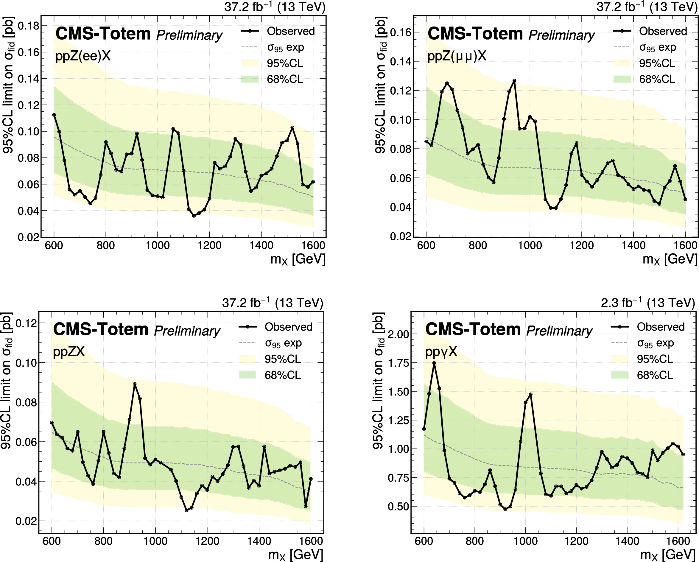
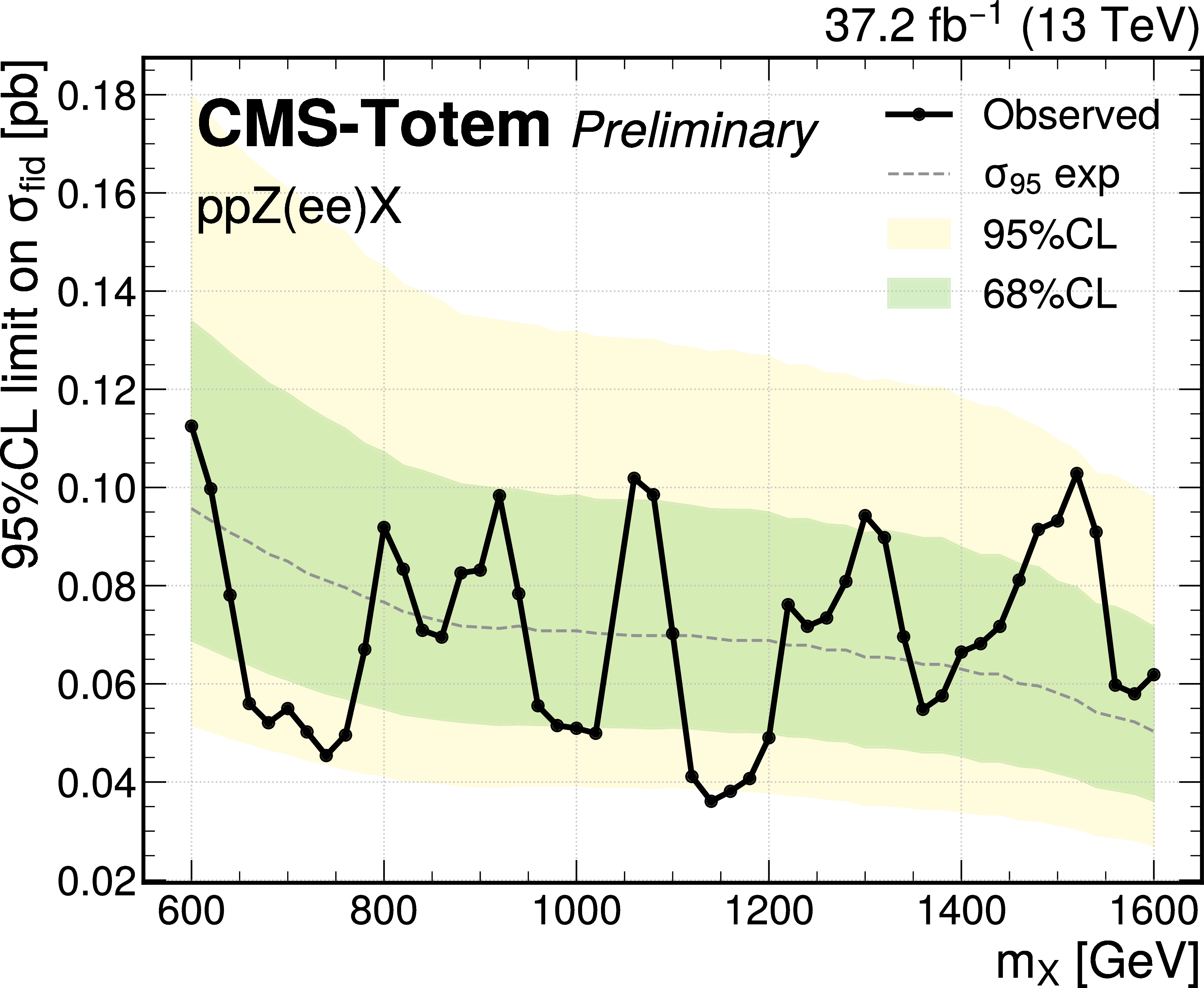
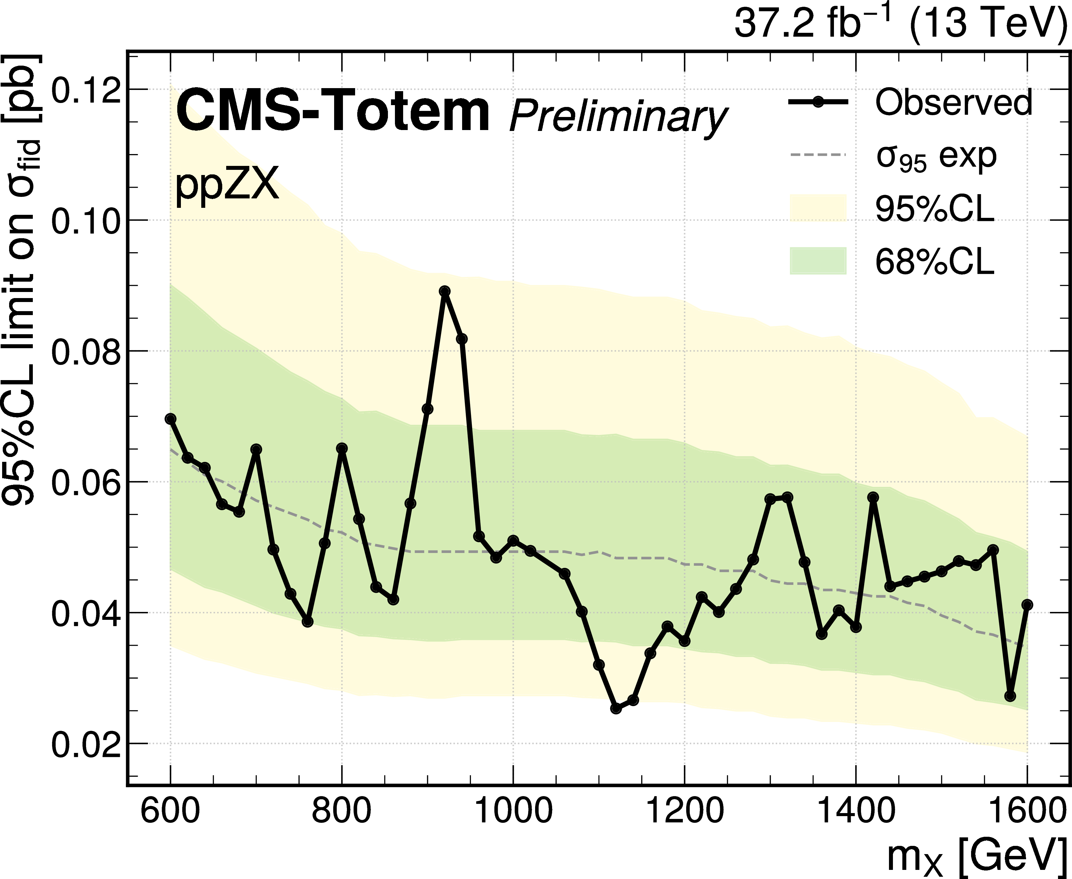
Figure 8:
Upper limits on the pp $\rightarrow$ pp Z/$\gamma$ X production cross section at the 95%, as function of $m_{X}$. The 95% and 68% CL quantiles of the expected limits are represented by the bands, while the observed limit is superimposed as a curve. The top plots correspond to the Z $ \rightarrow $ ee and Z $ \rightarrow \mu \mu $ final states, while the bottom plots correspond to the combined Z and $\gamma $ analyses. |
png pdf |
Figure 8-a:
Upper limits on the pp $\rightarrow$ pp Z/$\gamma$ X production cross section at the 95%, as function of $m_{X}$. The 95% and 68% CL quantiles of the expected limits are represented by the bands, while the observed limit is superimposed as a curve. The top plots correspond to the Z $ \rightarrow $ ee and Z $ \rightarrow \mu \mu $ final states, while the bottom plots correspond to the combined Z and $\gamma $ analyses. |

png pdf |
Figure 8-b:
Upper limits on the pp $\rightarrow$ pp Z/$\gamma$ X production cross section at the 95%, as function of $m_{X}$. The 95% and 68% CL quantiles of the expected limits are represented by the bands, while the observed limit is superimposed as a curve. The top plots correspond to the Z $ \rightarrow $ ee and Z $ \rightarrow \mu \mu $ final states, while the bottom plots correspond to the combined Z and $\gamma $ analyses. |
png pdf |
Figure 8-c:
Upper limits on the pp $\rightarrow$ pp Z/$\gamma$ X production cross section at the 95%, as function of $m_{X}$. The 95% and 68% CL quantiles of the expected limits are represented by the bands, while the observed limit is superimposed as a curve. The top plots correspond to the Z $ \rightarrow $ ee and Z $ \rightarrow \mu \mu $ final states, while the bottom plots correspond to the combined Z and $\gamma $ analyses. |
png pdf |
Figure 8-d:
Upper limits on the pp $\rightarrow$ pp Z/$\gamma$ X production cross section at the 95%, as function of $m_{X}$. The 95% and 68% CL quantiles of the expected limits are represented by the bands, while the observed limit is superimposed as a curve. The top plots correspond to the Z $ \rightarrow $ ee and Z $ \rightarrow \mu \mu $ final states, while the bottom plots correspond to the combined Z and $\gamma $ analyses. |
| Tables | |
png pdf |
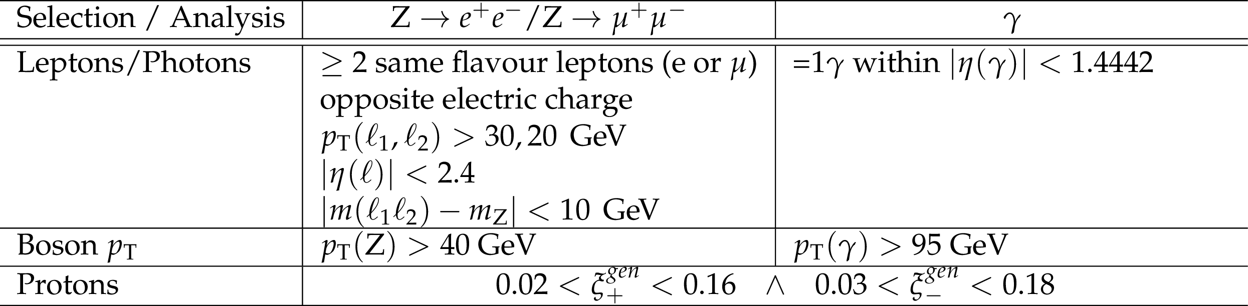
Table 1:
Combined CMS+Totem fiducial volume selection criteria in the Z and $\gamma $ analysis. |
| Summary |
| A search is presented for anomalous central exclusive Z/$\gamma$+X production using up to 37.2 fb$^{-1}$ of data recorded in 2017 by the CMS detector and the CMS-TOTEM precision proton spectrometer. A hypothetical X resonance is searched for in the mass region between 0.6 and 1.6 TeV, with cuts optimised for the best expected significance. Benefiting from the excellent mass resolution of 2% offered by the combination of the CMS central detector and the CT-PPS, for the first time at the LHC, the missing mass distribution is used to perform a model-independent search. Upper limits on the visible cross section of the pp $\rightarrow$ pp $+$ Z/$\gamma$ $+$ X process are set in a fiducial volume, using a generic model, in the absence of significant deviations in data with respect to the background predictions. With these results we demonstrate the feasibility of missing mass-based searches at the LHC. |
| References | ||||
| 1 | ATLAS Collaboration | A strategy for a general search for new phenomena using data-derived signal regions and its application within the ATLAS experiment | EPJC 79 (2019), no. 2, 120 | 1807.07447 |
| 2 | CMS Collaboration | MUSiC: a model-unspecific search for new physics in proton-proton collisions at $ \sqrt{s} = $ 13 TeV | EPJC 81 (2021), no. 7, 629 | CMS-EXO-19-008 2010.02984 |
| 3 | ATLAS Collaboration | Search for new phenomena in three- or four-lepton events in pp collisions at s=13 TeV with the ATLAS detector | PLB 824 (2022) 136832 | 2107.00404 |
| 4 | G. Karagiorgi et al. | Machine Learning in the Search for New Fundamental Physics | 2112.03769 | |
| 5 | W. Buchmuller and D. Wyler | Effective Lagrangian Analysis of New Interactions and Flavor Conservation | NPB 268 (1986) 621--653 | |
| 6 | B. Grzadkowski, M. Iskrzynski, M. Misiak, and J. Rosiek | Dimension-Six Terms in the Standard Model Lagrangian | JHEP 10 (2010) 085 | 1008.4884 |
| 7 | J. Ellis et al. | Top, Higgs, Diboson and Electroweak Fit to the Standard Model Effective Field Theory | JHEP 04 (2021) 279 | 2012.02779 |
| 8 | SMEFiT Collaboration | Combined SMEFT interpretation of Higgs, diboson, and top quark data from the LHC | JHEP 11 (2021) 089 | 2105.00006 |
| 9 | CMS Collaboration | The CMS experiment at the CERN LHC | JINST 3 (2008) S08004 | CMS-00-001 |
| 10 | CMS and TOTEM Collaborations | CMS-TOTEM Precision Proton Spectrometer | CERN-LHCC-2014-021, TOTEM-TDR-003, CMS-TDR-13 | |
| 11 | CMS Collaboration | Performance of the CMS Level-1 trigger in proton-proton collisions at $ \sqrt{s} = $ 13 TeV | JINST 15 (2020) P10017 | CMS-TRG-17-001 2006.10165 |
| 12 | CMS Collaboration | The CMS trigger system | JINST 12 (2017) P01020 | CMS-TRG-12-001 1609.02366 |
| 13 | CMS, TOTEM Collaboration | Proton reconstruction with the Precision Proton Spectrometer in Run 2 | ||
| 14 | CMS Collaboration | Proton reconstruction with the Precision Proton Spectrometer (PPS) in Run 2 | CDS | |
| 15 | CMS Collaboration | Efficiency of the Si-strips sensors used in the Precision Proton Spectrometer: radiation damage | CDS | |
| 16 | CMS Collaboration | Efficiency of the Pixel sensors used in the Precision Proton Spectrometer: radiation damage | CDS | |
| 17 | CMS, TOTEM Collaboration | Observation of proton-tagged, central (semi)exclusive production of high-mass lepton pairs in pp collisions at 13 TeV with the CMS-TOTEM precision proton spectrometer | JHEP 07 (2018) 153 | 1803.04496 |
| 18 | V. M. Budnev, I. F. Ginzburg, G. V. Meledin, and V. G. Serbo | The Two photon particle production mechanism. Physical problems. Applications. Equivalent photon approximation | PR 15 (1975) 181--281 | |
| 19 | S. Agostinelli et al. | Geant4—a simulation toolkit | Nuclear Instruments and Methods in Physics Research Section A: Accelerators, Spectrometers, Detectors and Associated Equipment 506 (2003), no. 3, 250--303 | |
| 20 | R. Frederix and S. Frixione | Merging meets matching in MC@NLO | JHEP 12 (2012) 061 | 1209.6215 |
| 21 | J. Alwall et al. | Comparative study of various algorithms for the merging of parton showers and matrix elements in hadronic collisions | EPJC 53 (2008) 473--500 | 0706.2569 |
| 22 | E. Re | Single-top Wt-channel production matched with parton showers using the POWHEG method | EPJC 71 (2011) 1547 | 1009.2450 |
| 23 | S. Frixione, P. Nason, and G. Ridolfi | A Positive-weight next-to-leading-order Monte Carlo for heavy flavour hadroproduction | JHEP 09 (2007) 126 | 0707.3088 |
| 24 | T. Sjostrand et al. | An Introduction to PYTHIA 8.2 | CPC 191 (2015) 159--177 | 1410.3012 |
| 25 | B. E. Cox and J. R. Forshaw | POMWIG: HERWIG for diffractive interactions | CPC 144 (2002) 104--110 | hep-ph/0010303 |
| 26 | CMS Collaboration | Particle-flow reconstruction and global event description with the CMS detector | JINST 12 (2017) P10003 | CMS-PRF-14-001 1706.04965 |
| 27 | L. Moneta et al. | The RooStats project | in 13$^\textth$ International Workshop on Advanced Computing and Analysis Techniques in Physics Research (ACAT2010) SISSA, 2010 PoS(ACAT2010)057 | 1009.1003 |
| 28 | B. Todd, L. Ponce, A. Apollonio, and D. J. Walsh | LHC Availability 2017: Technical Stop 2 to End of Standard Proton Physics | technical report, Dec | |
| 29 | CMS Collaboration | CMS luminosity measurement for the 2017 data-taking period at $ \sqrt{s} = $ 13 TeV | CMS-PAS-LUM-17-004 | CMS-PAS-LUM-17-004 |
| 30 | R. J. Barlow and C. Beeston | Fitting using finite Monte Carlo samples | CPC 77 (1993) 219--228 | |
| 31 | T. Junk | Confidence level computation for combining searches with small statistics | NIMA 434 (1999) 435--443 | hep-ex/9902006 |
| 32 | A. L. Read | Presentation of search results: the CL$ _{\rm s} $ technique | Journal of Physics G: Nuclear and Particle Physics 28 (sep, 2002) 2693--2704 | |
| 33 | ATLAS, CMS, LHC Higgs Combination Group Collaboration | Procedure for the LHC Higgs boson search combination in Summer 2011 | CMS-NOTE-2011-005 | |
| 34 | G. Cowan, K. Cranmer, E. Gross, and O. Vitells | Asymptotic formulae for likelihood-based tests of new physics | EPJC 71 (2011) 1554 | 1007.1727 |
|
|
Compact Muon Solenoid LHC, CERN |
|

|

|

|

|

|