

Compact Muon Solenoid
LHC, CERN
| CMS-PAS-EXO-19-005 | ||
| Search for long-lived particles using delayed photons with proton-proton collisions at $\sqrt{s}= $ 13 TeV | ||
| CMS Collaboration | ||
| July 2019 | ||
| Abstract: A search for new physics with long-lived particles decaying to photons is presented using proton-proton collisions data at $\sqrt{s}= $ 13 TeV collected by the CMS experiment in 2016 and 2017 corresponding to 35.9 fb$^{-1}$ and 41.5 fb$^{-1}$ of integrated luminosity, respectively. Results are interpreted in the context of supersymmetry with gauge-mediated supersymmetry breaking, where long-lived neutralinos are produced as secondaries and decay to a photon and a gravitino. Limits are presented as a function of the neutralino proper decay length and mass. For neutralino proper decay lengths of 10$^{1}$, 10$^{2}$, 10$^{3}$, and 10$^{4} $ cm, masses up to 320, 525, 360, and 215 GeV are excluded at 95% CL, respectively. We extend the previous best limits in the neutralino proper decay length by up to about one order of magnitude, and in neutralino mass by up to about 100 GeV. | ||
|
Links:
CDS record (PDF) ;
CADI line (restricted) ;
These preliminary results are superseded in this paper, PRD 100 (2019) 112003. The superseded preliminary plots can be found here. |
||
| Figures & Tables | Summary | Additional Figures & Tables | References | CMS Publications |
|---|
| Figures | |
png pdf |
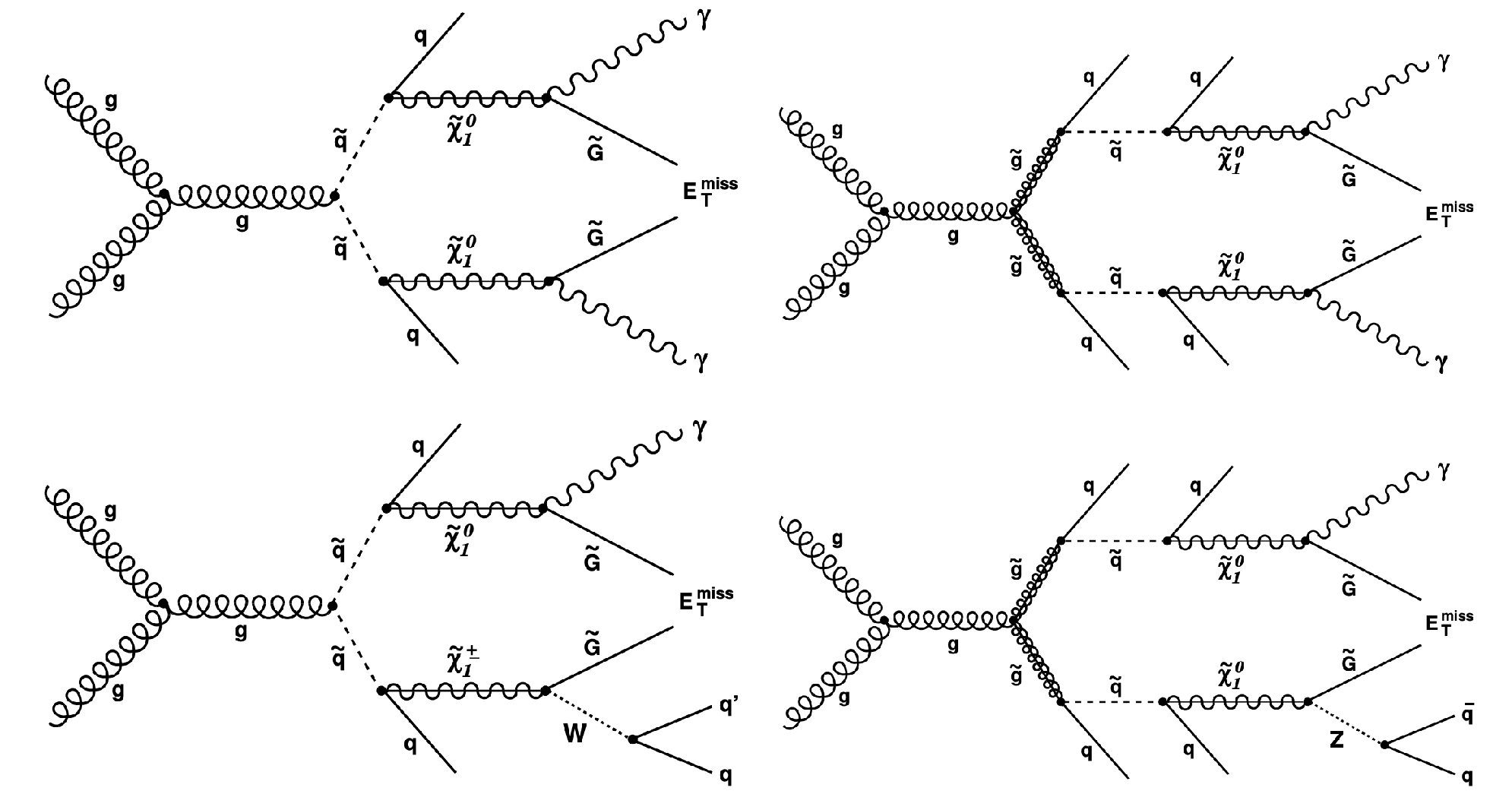
Figure 1:
Example diagrams for SUSY processes that result in a diphoton (top) and single photon (bottom) final state through squark (left) and gluino (right) pair-production at the LHC. |
png pdf |
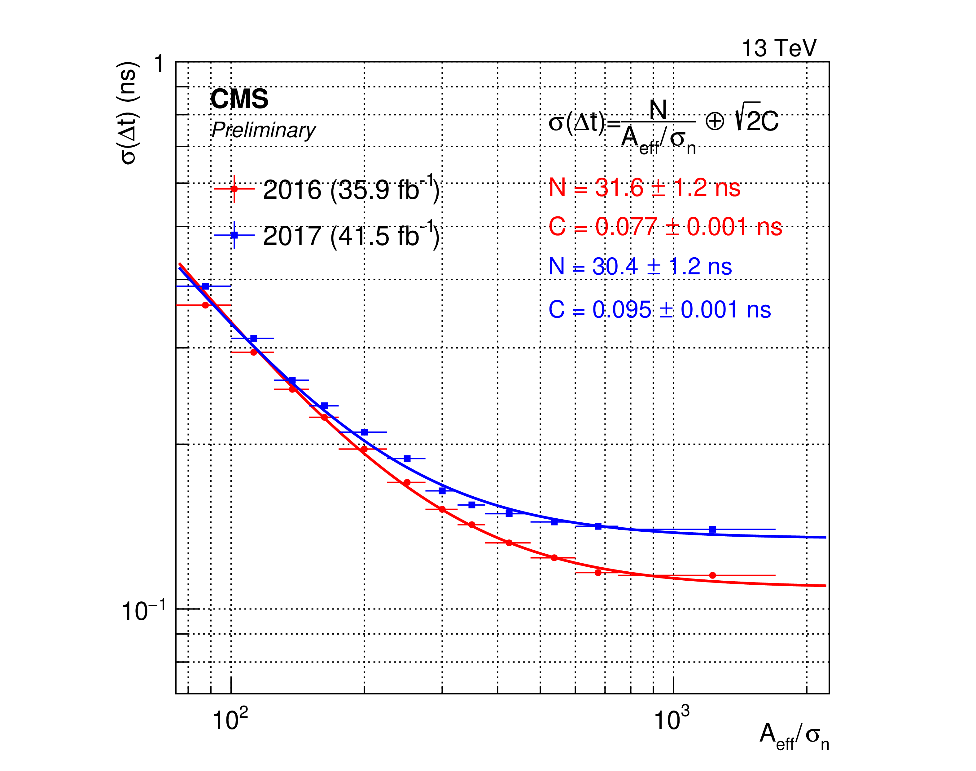
Figure 2:
The time resolution between two neighboring ECAL crystals as a function of the effective amplitudes of the signals in the two crystals is shown for the 2016 and 2017 data sets. |
png pdf |
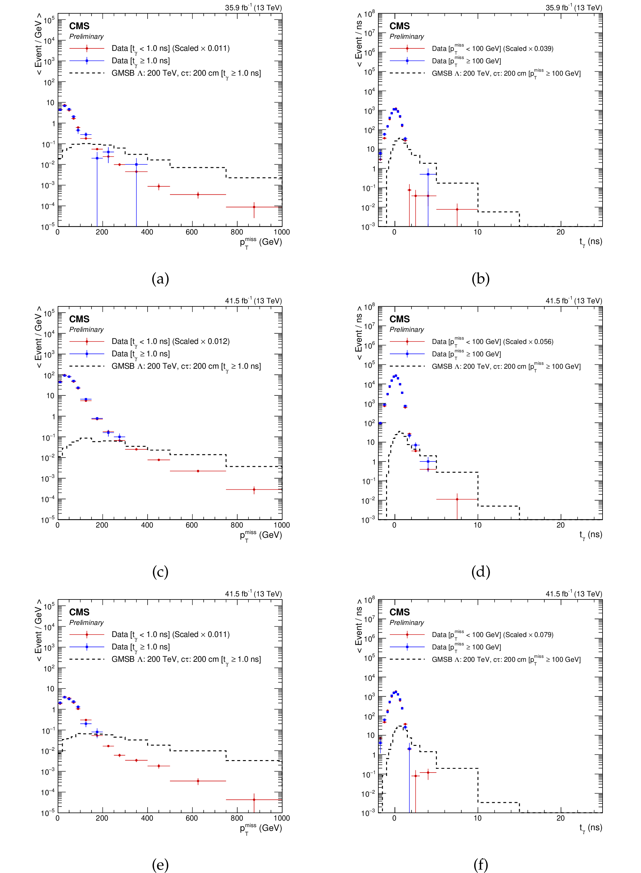
Figure 3:
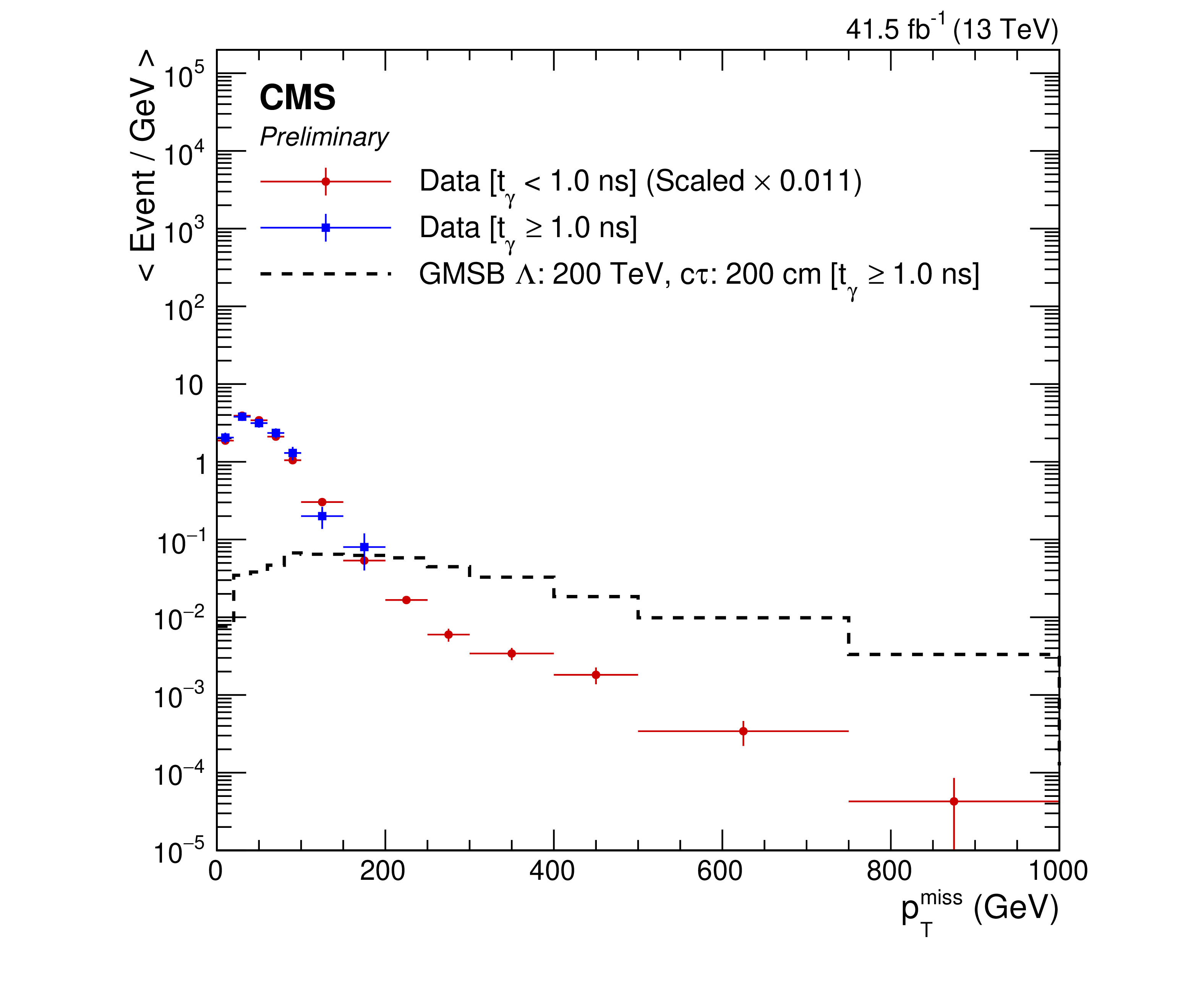
Distributions of the number events in data and a representative signal point (GMSB: $\Lambda =$ 200 TeV, ${c\tau} =$ 200 cm ) scaled by the production cross section times the integrated luminosity as functions of ${{p_{\mathrm {T}}} ^\text {miss}}$ (a, c, e) and ${t_{\gamma}}$ (b, d, f) using the 2016 (a, b), 2017$\gamma$ (c, d) and 2017$\gamma \gamma$ (e, f) event selections. The ${{p_{\mathrm {T}}} ^\text {miss}}$ distribution in data is split for events with $ {t_{\gamma}} < $ 1 ns (red, scaled down to match the total number of events with $ {t_{\gamma}}\geq $ 1 ns) and $ {t_{\gamma}}\geq $ 1 ns (blue), while the signal (black) is shown for late times. The ${t_{\gamma}}$ distribution in data is split for events with $ {{p_{\mathrm {T}}} ^\text {miss}} < $ 100 GeV (red, scaled down to match the total number of events with $ {{p_{\mathrm {T}}} ^\text {miss}} \geq $ 100 GeV) and $ {{p_{\mathrm {T}}} ^\text {miss}} \geq $ 100 GeV (blue), while the signal (black) is shown for high ${{p_{\mathrm {T}}} ^\text {miss}}$. The entries in each bin are normalized by the bin width, where the horizontal bars on data indicate the bin boundaries. The last bin in each plot contains overflow events. |

png pdf |
Figure 3-a:
Distribution of the number events in data and a representative signal point (GMSB: $\Lambda =$ 200 TeV, ${c\tau} =$ 200 cm ) scaled by the production cross section times the integrated luminosity as a function of ${{p_{\mathrm {T}}} ^\text {miss}}$ using the 2016 event selection. The ${{p_{\mathrm {T}}} ^\text {miss}}$ distribution in data is split for events with $ {t_{\gamma}} < $ 1 ns (red, scaled down to match the total number of events with $ {t_{\gamma}}\geq $ 1 ns) and $ {t_{\gamma}}\geq $ 1 ns (blue), while the signal (black) is shown for late times. The ${t_{\gamma}}$ distribution in data is split for events with $ {{p_{\mathrm {T}}} ^\text {miss}} < $ 100 GeV (red, scaled down to match the total number of events with $ {{p_{\mathrm {T}}} ^\text {miss}} \geq $ 100 GeV) and $ {{p_{\mathrm {T}}} ^\text {miss}} \geq $ 100 GeV (blue), while the signal (black) is shown for high ${{p_{\mathrm {T}}} ^\text {miss}}$. The entries in each bin are normalized by the bin width, where the horizontal bars on data indicate the bin boundaries. The last bin contains overflow events. |
png pdf |
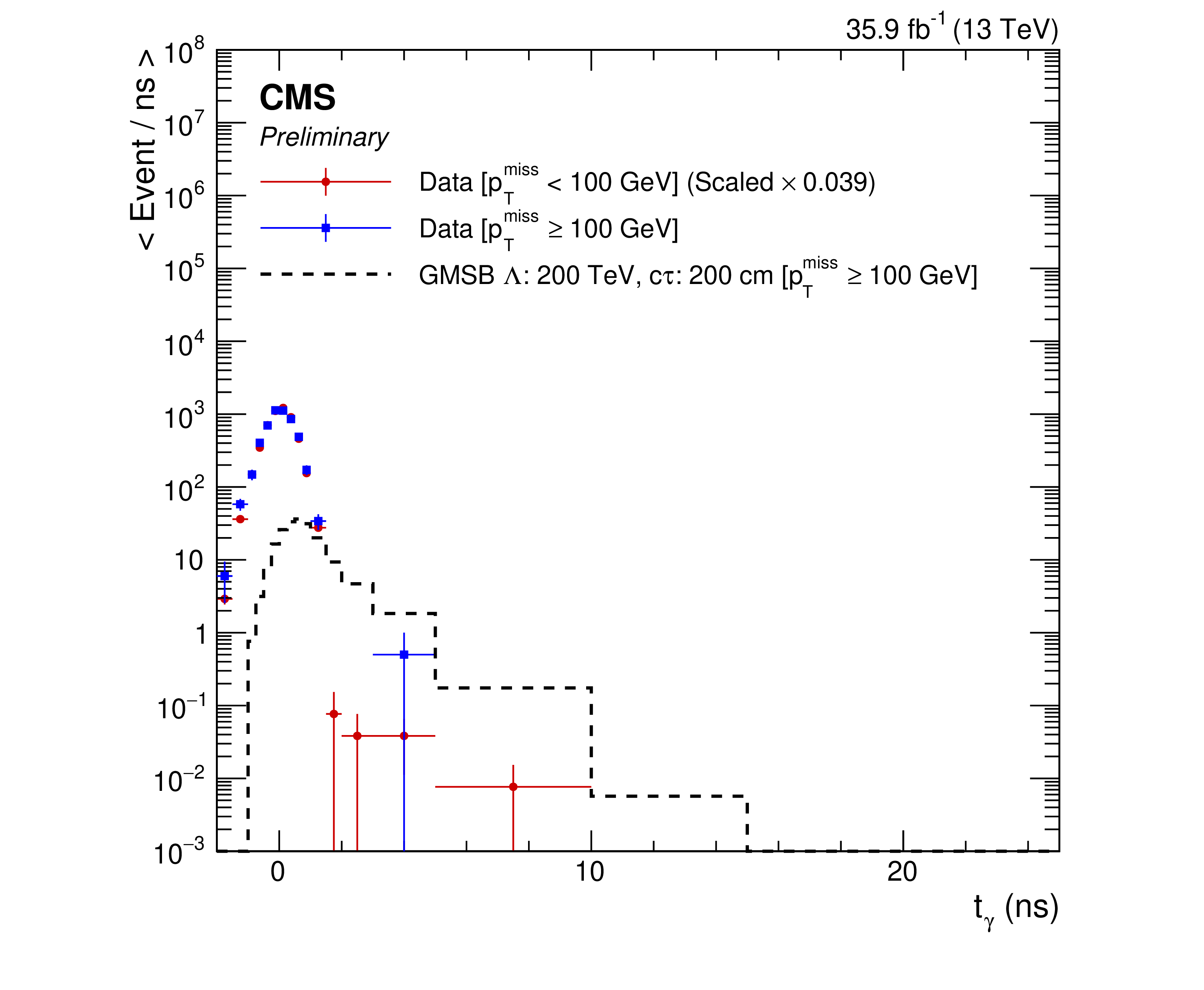
Figure 3-b:
Distribution of the number events in data and a representative signal point (GMSB: $\Lambda =$ 200 TeV, ${c\tau} =$ 200 cm ) scaled by the production cross section times the integrated luminosity as a function of ${t_{\gamma}}$ using the 2016 event selection. The ${{p_{\mathrm {T}}} ^\text {miss}}$ distribution in data is split for events with $ {t_{\gamma}} < $ 1 ns (red, scaled down to match the total number of events with $ {t_{\gamma}}\geq $ 1 ns) and $ {t_{\gamma}}\geq $ 1 ns (blue), while the signal (black) is shown for late times. The ${t_{\gamma}}$ distribution in data is split for events with $ {{p_{\mathrm {T}}} ^\text {miss}} < $ 100 GeV (red, scaled down to match the total number of events with $ {{p_{\mathrm {T}}} ^\text {miss}} \geq $ 100 GeV) and $ {{p_{\mathrm {T}}} ^\text {miss}} \geq $ 100 GeV (blue), while the signal (black) is shown for high ${{p_{\mathrm {T}}} ^\text {miss}}$. The entries in each bin are normalized by the bin width, where the horizontal bars on data indicate the bin boundaries. The last bin contains overflow events. |

png pdf |
Figure 3-c:
Distribution of the number events in data and a representative signal point (GMSB: $\Lambda =$ 200 TeV, ${c\tau} =$ 200 cm ) scaled by the production cross section times the integrated luminosity as a function of ${{p_{\mathrm {T}}} ^\text {miss}}$ using the 2017$\gamma$ event selection. The ${{p_{\mathrm {T}}} ^\text {miss}}$ distribution in data is split for events with $ {t_{\gamma}} < $ 1 ns (red, scaled down to match the total number of events with $ {t_{\gamma}}\geq $ 1 ns) and $ {t_{\gamma}}\geq $ 1 ns (blue), while the signal (black) is shown for late times. The ${t_{\gamma}}$ distribution in data is split for events with $ {{p_{\mathrm {T}}} ^\text {miss}} < $ 100 GeV (red, scaled down to match the total number of events with $ {{p_{\mathrm {T}}} ^\text {miss}} \geq $ 100 GeV) and $ {{p_{\mathrm {T}}} ^\text {miss}} \geq $ 100 GeV (blue), while the signal (black) is shown for high ${{p_{\mathrm {T}}} ^\text {miss}}$. The entries in each bin are normalized by the bin width, where the horizontal bars on data indicate the bin boundaries. The last bin contains overflow events. |

png pdf |
Figure 3-d:
Distribution of the number events in data and a representative signal point (GMSB: $\Lambda =$ 200 TeV, ${c\tau} =$ 200 cm ) scaled by the production cross section times the integrated luminosity as a function of ${t_{\gamma}}$ using the 2017$\gamma$ event selection. The ${{p_{\mathrm {T}}} ^\text {miss}}$ distribution in data is split for events with $ {t_{\gamma}} < $ 1 ns (red, scaled down to match the total number of events with $ {t_{\gamma}}\geq $ 1 ns) and $ {t_{\gamma}}\geq $ 1 ns (blue), while the signal (black) is shown for late times. The ${t_{\gamma}}$ distribution in data is split for events with $ {{p_{\mathrm {T}}} ^\text {miss}} < $ 100 GeV (red, scaled down to match the total number of events with $ {{p_{\mathrm {T}}} ^\text {miss}} \geq $ 100 GeV) and $ {{p_{\mathrm {T}}} ^\text {miss}} \geq $ 100 GeV (blue), while the signal (black) is shown for high ${{p_{\mathrm {T}}} ^\text {miss}}$. The entries in each bin are normalized by the bin width, where the horizontal bars on data indicate the bin boundaries. The last bin contains overflow events. |
png pdf |
Figure 3-e:
Distribution of the number events in data and a representative signal point (GMSB: $\Lambda =$ 200 TeV, ${c\tau} =$ 200 cm ) scaled by the production cross section times the integrated luminosity as a function of ${{p_{\mathrm {T}}} ^\text {miss}}$ using the 2017$\gamma \gamma$ event selection. The ${{p_{\mathrm {T}}} ^\text {miss}}$ distribution in data is split for events with $ {t_{\gamma}} < $ 1 ns (red, scaled down to match the total number of events with $ {t_{\gamma}}\geq $ 1 ns) and $ {t_{\gamma}}\geq $ 1 ns (blue), while the signal (black) is shown for late times. The ${t_{\gamma}}$ distribution in data is split for events with $ {{p_{\mathrm {T}}} ^\text {miss}} < $ 100 GeV (red, scaled down to match the total number of events with $ {{p_{\mathrm {T}}} ^\text {miss}} \geq $ 100 GeV) and $ {{p_{\mathrm {T}}} ^\text {miss}} \geq $ 100 GeV (blue), while the signal (black) is shown for high ${{p_{\mathrm {T}}} ^\text {miss}}$. The entries in each bin are normalized by the bin width, where the horizontal bars on data indicate the bin boundaries. The last bin contains overflow events. |

png pdf |
Figure 3-f:
Distribution of the number events in data and a representative signal point (GMSB: $\Lambda =$ 200 TeV, ${c\tau} =$ 200 cm ) scaled by the production cross section times the integrated luminosity as a function of ${{p_{\mathrm {T}}} ^\text {miss}}$ using the 2017$\gamma \gamma$ event selection. The ${{p_{\mathrm {T}}} ^\text {miss}}$ distribution in data is split for events with $ {t_{\gamma}} < $ 1 ns (red, scaled down to match the total number of events with $ {t_{\gamma}}\geq $ 1 ns) and $ {t_{\gamma}}\geq $ 1 ns (blue), while the signal (black) is shown for late times. The ${t_{\gamma}}$ distribution in data is split for events with $ {{p_{\mathrm {T}}} ^\text {miss}} < $ 100 GeV (red, scaled down to match the total number of events with $ {{p_{\mathrm {T}}} ^\text {miss}} \geq $ 100 GeV) and $ {{p_{\mathrm {T}}} ^\text {miss}} \geq $ 100 GeV (blue), while the signal (black) is shown for high ${{p_{\mathrm {T}}} ^\text {miss}}$. The entries in each bin are normalized by the bin width, where the horizontal bars on data indicate the bin boundaries. The last bin contains overflow events. |
png pdf |
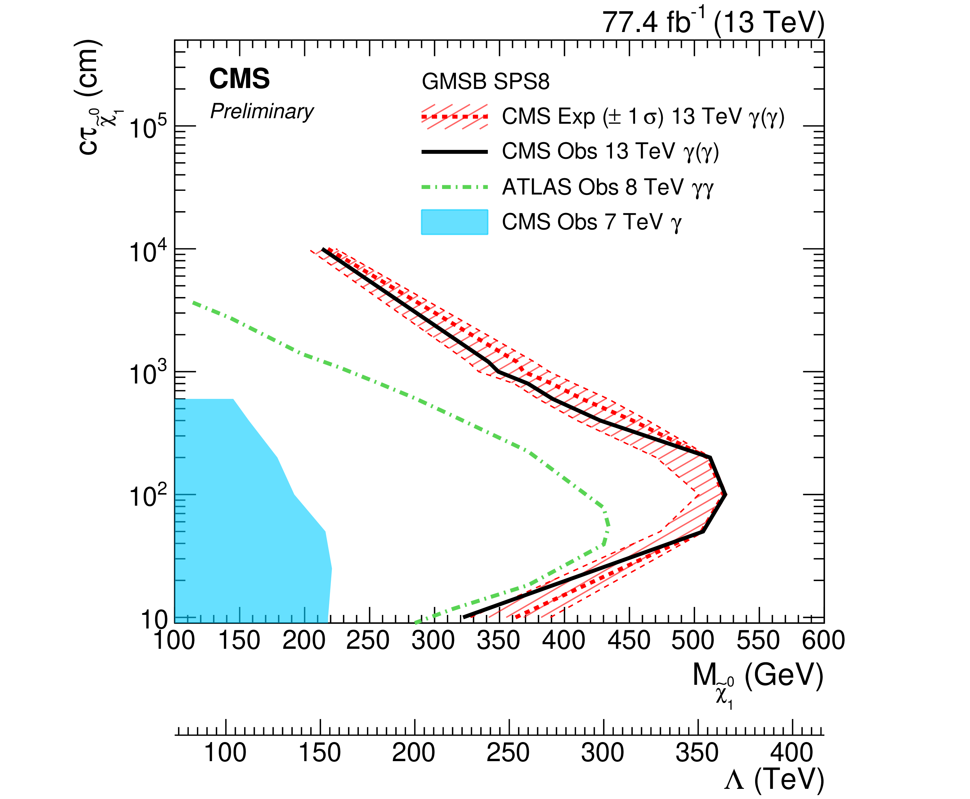
Figure 4:
The observed 95% CL exclusion contours on the signal production cross section are shown as a function of the neutralino proper decay length $c\tau _{\tilde{\chi}^0_1}$ versus the neutralino mass in the GMSB SPS8 model. |
| Tables | |
png pdf |
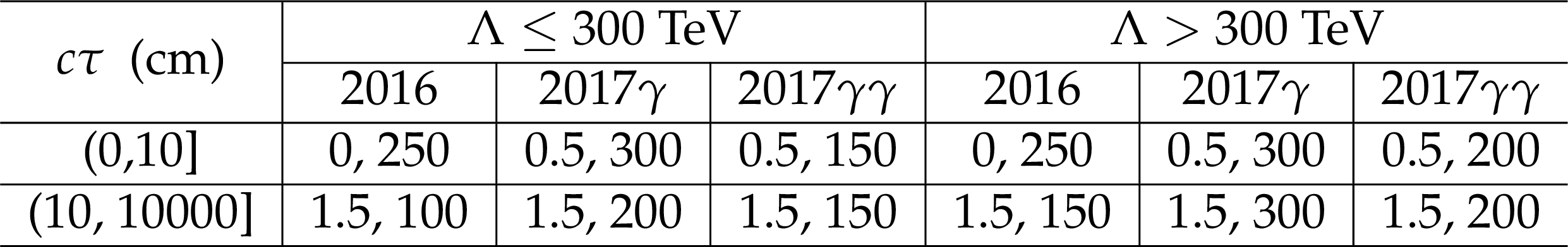
Table 1:
The optimized bin boundaries for the ${t_{\gamma}}$ (first number in units of ns) and ${{p_{\mathrm {T}}} ^\text {miss}}$ (second number in units of GeV) are shown for different GMSB SPS8 signal model parameter space points considered in the search for each data set category. |

png pdf |
Table 2:
Summary table of systematics and their assigned values in this analysis. Also included are notes on whether each source affects signal yields (Sig) or background (Bkg) estimates, to which bins each uncertainty applies, and how the correlations of the uncertainties between the different data sets are treated. We assign different values for the uncertainty on the closure of the background prediction for short and long lifetime signal models. |
png pdf |
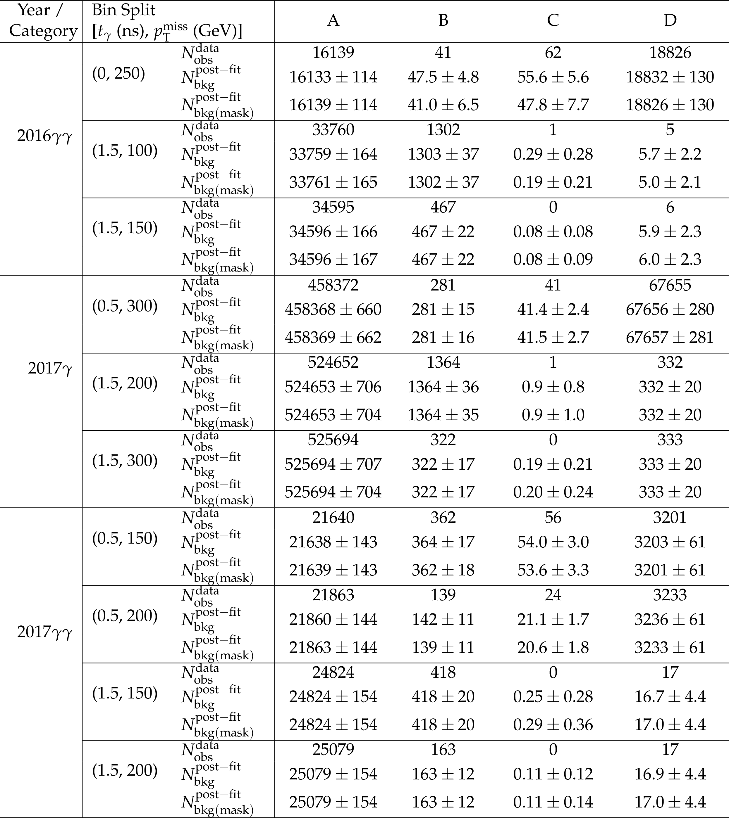
Table 3:
Observed events (${N_{\mathrm {obs}}^{\mathrm {data}}}$) and predicted background post-fit yields from background-only fit (${N_{\mathrm {bkg}}^{\mathrm {post-fit}}}$) in bins A, B, C and D for data from different years and categories and for different ${t_{\gamma}}$ and ${{p_{\mathrm {T}}} ^\text {miss}}$ split options. In addition, the predicted post-fit yields from the background-only fit masking bin C (${N_{\mathrm {bkg(mask)}}^{\mathrm {post-fit}}}$) are provided as a test of closure. Uncertainties for ${N_{\mathrm {bkg}}^{\mathrm {post-fit}}}$ and ${N_{\mathrm {bkg(mask)}}^{\mathrm {post-fit}}}$ are the sum in quadrature of the statistical and systematic uncertainties (statistical uncertainties dominate). |
| Summary |
| A search for long-lived particles (LLP) decaying to a photon and a weakly-interacting particle using proton-proton collisions at a center of mass energy of 13 TeV collected by the CMS experiment is presented. Such photons impact the electromagnetic calorimeter at a nonnormal impact angles and at delayed times, and this striking combination of features is exploited to suppress backgrounds. The search is performed using a combination of the 2016 and 2017 data sets, corresponding to a total integrated luminosity of 77.4 fb$^{-1}$. A combination of single photon and diphoton events is used for the search, which yields complementary sensitivity at larger and smaller LLP proper decay lengths, respectively. The results are interpreted in the context of supersymmetry with gauge-mediated SUSY breaking using the SPS8 benchmark model. For neutralino proper decay lengths of $10^1$, $10^2$, $10^3$, and $10^4$ cm, masses up to about 320, 525, 360, and 215 GeV are excluded at 95% CL, respectively. The previous best limits are extended by about one order of magnitude in the neutralino proper decay length, and the mass reach is improved by about 100 GeV. |
| Additional Figures | |
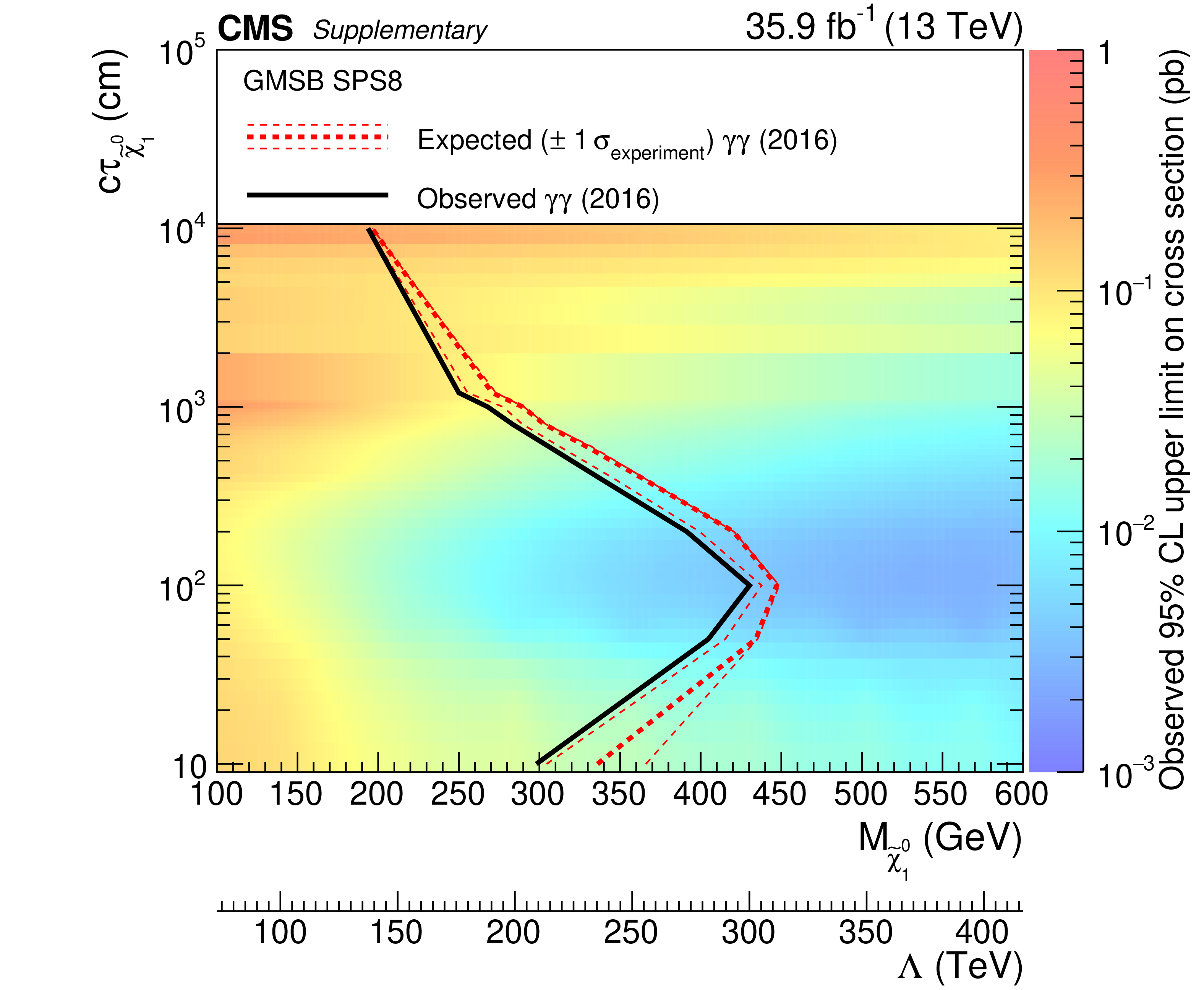
png pdf |
Additional Figure 1:
The observed 2016 category upper limits at 95% CL on the GMSB SPS8 signal cross section, as a function of neutralino mass and proper decay length. The area at the left of the black curve represents the observed exclusion region, while the dashed red lines represent the exclusion region from expected limits and their $ \pm $1 standard deviations. |
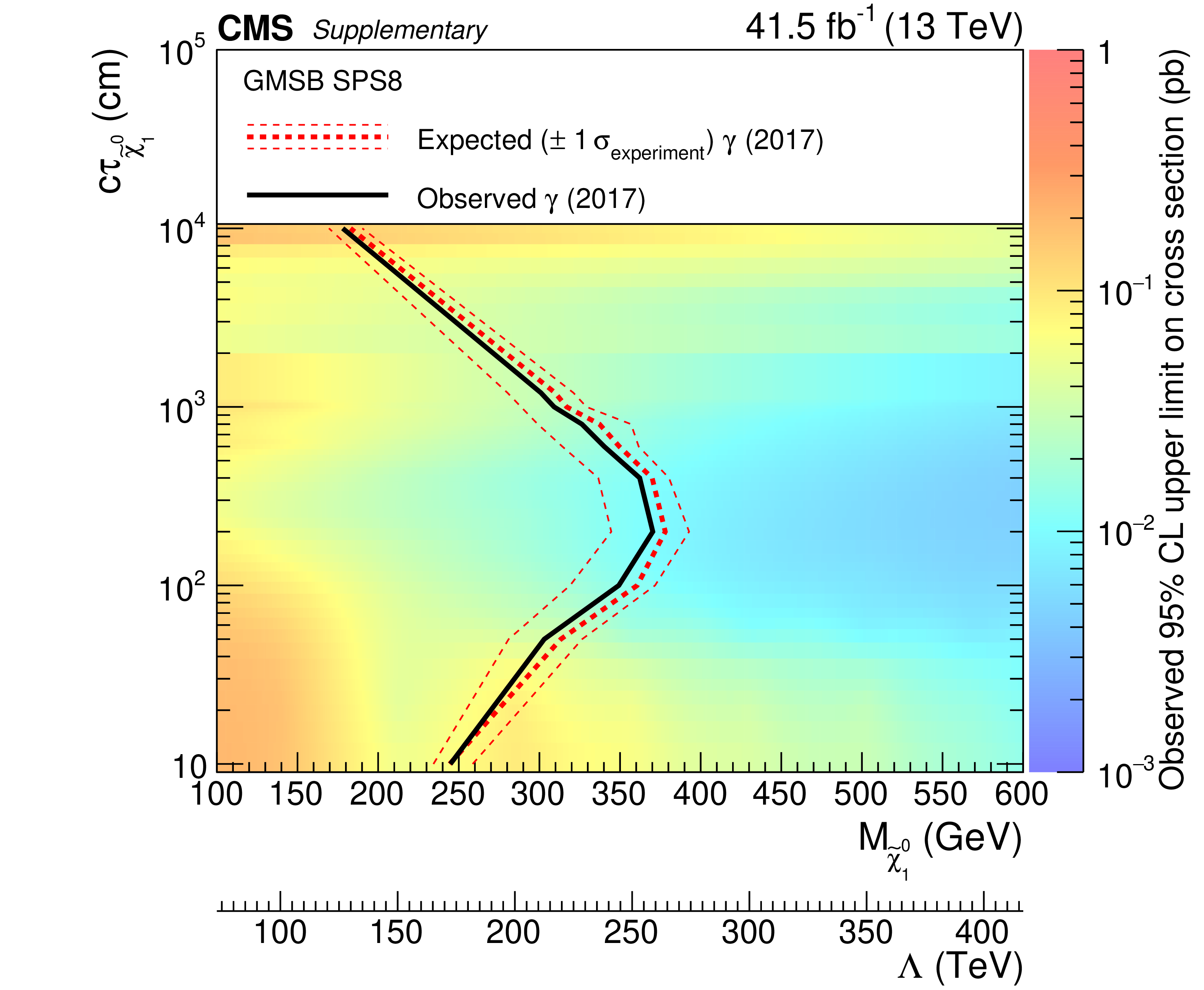
png pdf |
Additional Figure 2:
The observed 2017$\gamma $ category upper limits at 95% CL on the GMSB SPS8 signal cross section, as a function of neutralino mass and proper decay length. The area at the left of the black curve represents the observed exclusion region, while the dashed red lines represent the exclusion region from expected limits and their $ \pm $1 standard deviations. |

png pdf |
Additional Figure 3:
The observed 2017$\gamma \gamma $ category upper limits at 95% CL on the GMSB SPS8 signal cross section, as a function of neutralino mass and proper decay length. The area at the left of the black curve represents the observed exclusion region, while the dashed red lines represent the exclusion region from expected limits and their $ \pm $1 standard deviations. |
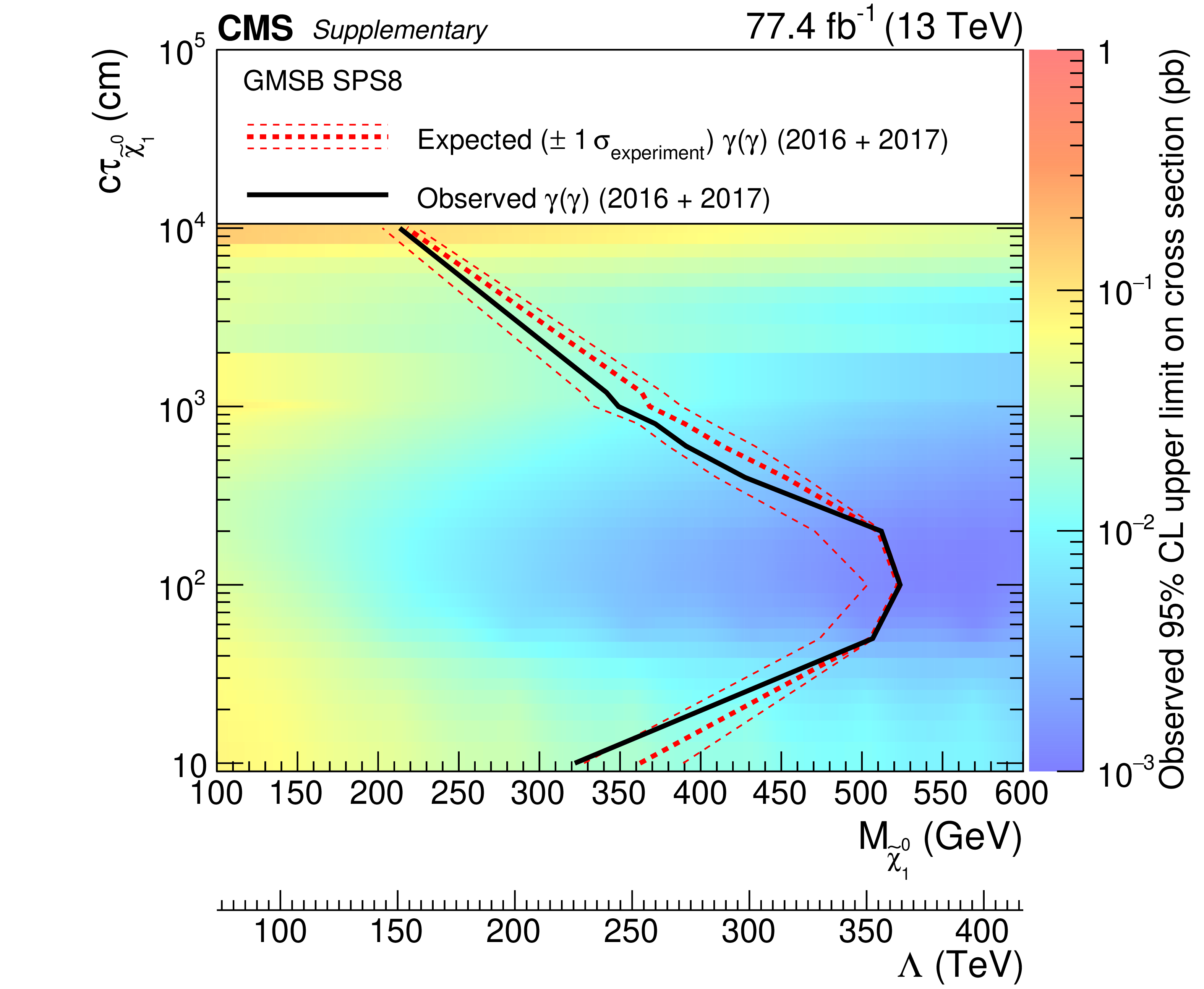
png pdf |
Additional Figure 4:
The observed 2016+2017 combined upper limits at 95% CL on the GMSB SPS8 signal cross section, as a function of neutralino mass and proper decay length. The area at the left of the black curve represents the observed exclusion region, while the dashed red lines represent the exclusion region from expected limits and their $ \pm $1 standard deviations. |

png pdf |
Additional Figure 5:
Event display of the observed event in bin C for 2017 using miniAOD. This event has $ {{p_{\mathrm {T}}} ^\text {miss}} = $ 268 GeV and $t_{\gamma}= $ 1.91 ns. Run number: 306423. Lumi section: 220. Event number: 388707708. |
| Additional Tables | |
png pdf |
Additional Table 1:
(2016) Event selection cut-flow efficiency for GMSB SPS8 $c\tau =$ 10 cm and varying $\Lambda $ (unit of efficiency:%; unit of $\Lambda $: TeV) using the 2016 event selection. |

png pdf |
Additional Table 2:
(2016) Event selection cut-flow efficiency for GMSB SPS8 $c\tau =$ 100 cm and varying $\Lambda $ (unit of efficiency:%; unit of $\Lambda $: TeV) using the 2016 event selection. |
png pdf |
Additional Table 3:
(2016) Event selection cut-flow efficiency for GMSB SPS8 $c\tau =$ 1000 cm and varying $\Lambda $ (unit of efficiency:%; unit of $\Lambda $: TeV) using the 2016 event selection. |
png pdf |
Additional Table 4:
(2016) Event selection cut-flow efficiency for GMSB SPS8 $c\tau =$ 10000 cm and varying $\Lambda $ (unit of efficiency:%; unit of $\Lambda $: TeV) using the 2016 event selection. |
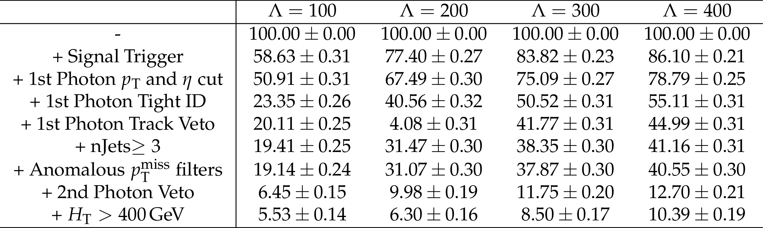
png pdf |
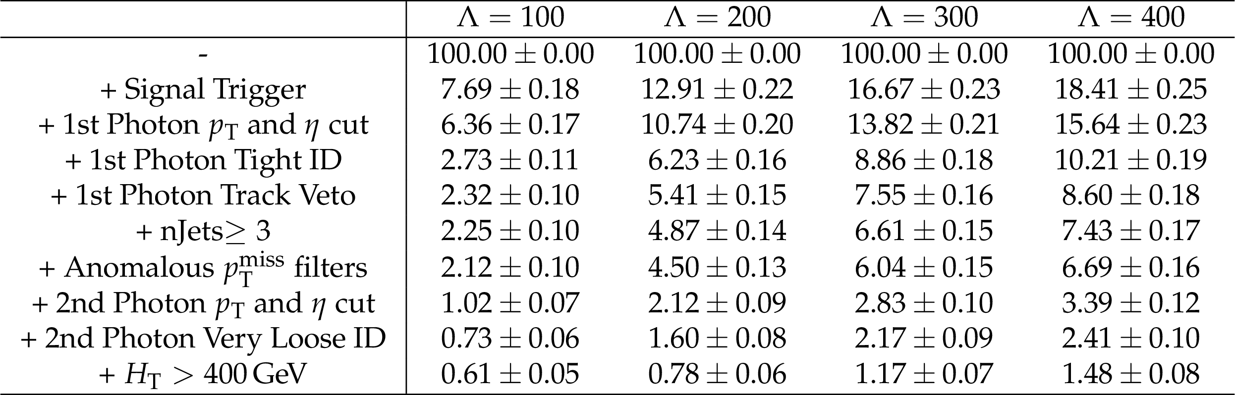
Additional Table 5:
(2017$\gamma $) Event selection cut-flow efficiency for GMSB SPS8 $c\tau =$ 10 cm and varying $\Lambda $ (unit of efficiency:%; unit of $\Lambda $: TeV) using the 2017$\gamma $ event selection. |

png pdf |
Additional Table 6:
(2017$\gamma $) Event selection cut-flow efficiency for GMSB SPS8 $c\tau =$ 100 cm and varying $\Lambda $ (unit of efficiency:%; unit of $\Lambda $: TeV) using the 2017$\gamma $ event selection. |
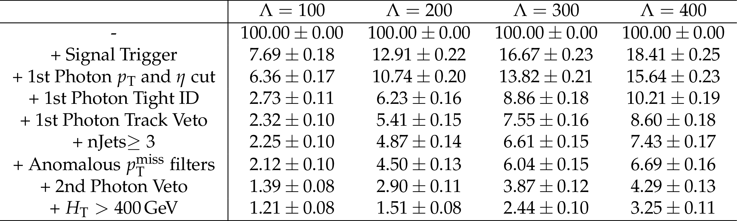
png pdf |
Additional Table 7:
(2017$\gamma $) Event selection cut-flow efficiency for GMSB SPS8 $c\tau =$ 1000 cm and varying $\Lambda $ (unit of efficiency:%; unit of $\Lambda $: TeV) using the 2017$\gamma $ event selection. |

png pdf |
Additional Table 8:
(2017$\gamma $) Event selection cut-flow efficiency for GMSB SPS8 $c\tau =$ 10000 cm and varying $\Lambda $ (unit of efficiency:%; unit of $\Lambda $: TeV) using the 2017$\gamma $ event selection. |

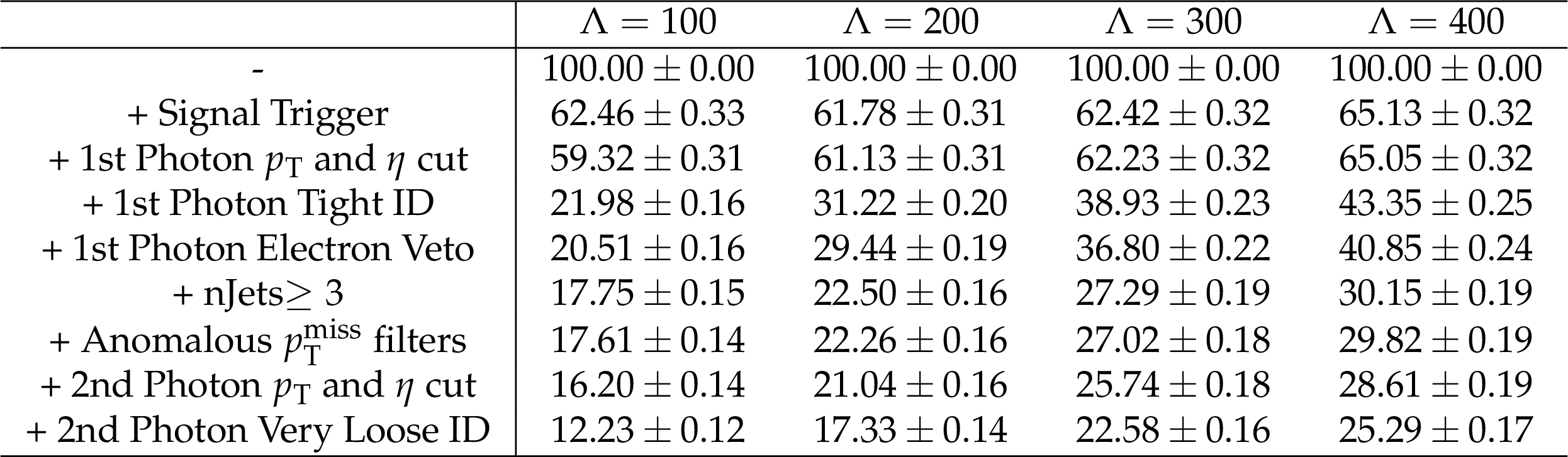
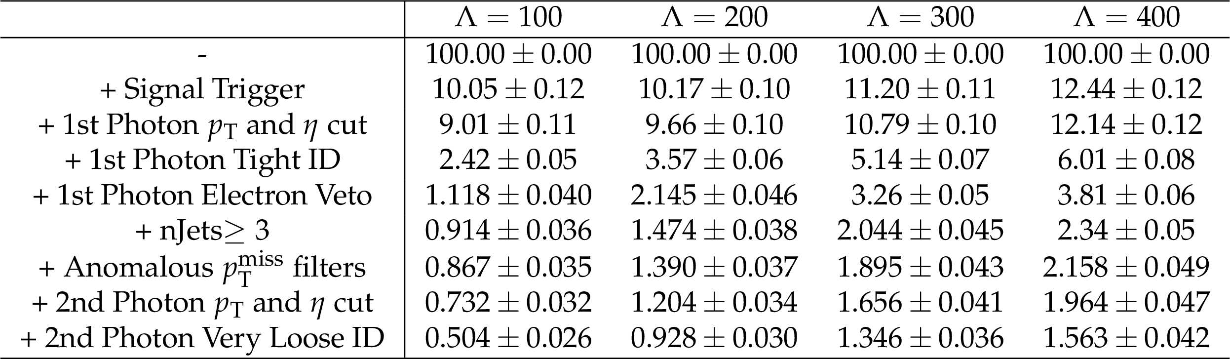
png pdf |
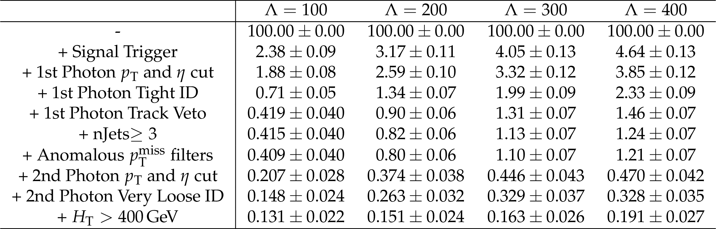
Additional Table 9:
(2017$\gamma \gamma $) Event selection cut-flow efficiency for GMSB SPS8 $c\tau =$ 10 cm and varying $\Lambda $ (unit of efficiency:%; unit of $\Lambda $: TeV) using the 2017$\gamma \gamma $ event selection. |

png pdf |
Additional Table 10:
(2017$\gamma \gamma $) Event selection cut-flow efficiency for GMSB SPS8 $c\tau =$ 100 cm and varying $\Lambda $ (unit of efficiency:%; unit of $\Lambda $: TeV) using the 2017$\gamma \gamma $ event selection. |
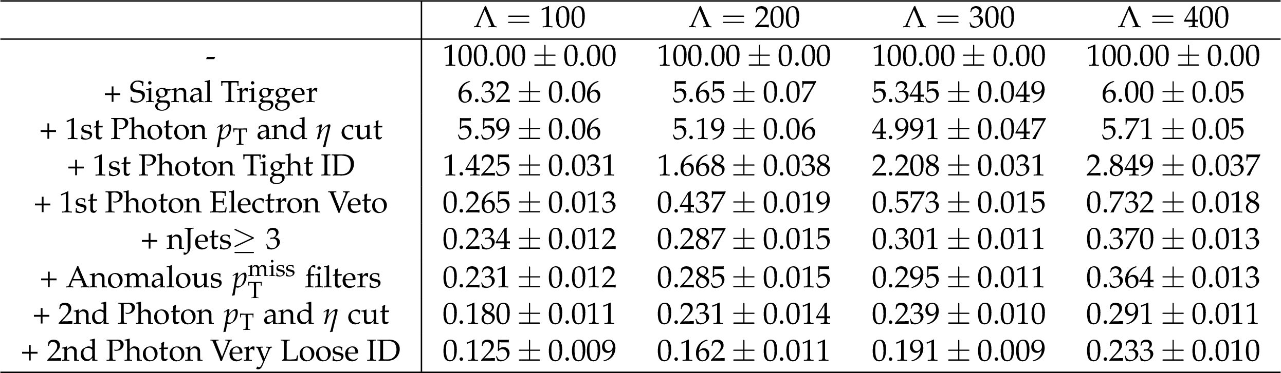
png pdf |
Additional Table 11:
(2017$\gamma \gamma $) Event selection cut-flow efficiency for GMSB SPS8 $c\tau =$ 1000 cm and varying $\Lambda $ (unit of efficiency:%; unit of $\Lambda $: TeV) using the 2017$\gamma \gamma $ event selection. |
png pdf |
Additional Table 12:
(2017$\gamma \gamma $) Event selection cut-flow efficiency for GMSB SPS8 $c\tau =$ 10000 cm and varying $\Lambda $ (unit of efficiency:%; unit of $\Lambda $: TeV) using the 2017$\gamma \gamma $ event selection. |
png pdf |
Additional Table 13:
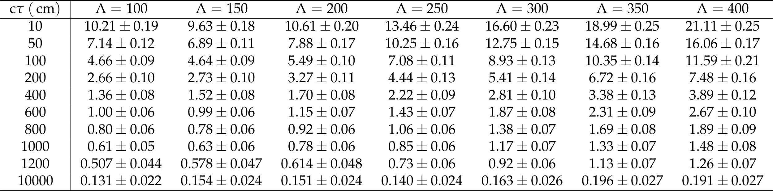
(2016) Event selection efficiency times acceptance for the GMSB SPS8 grid points used in the analysis (unit of efficiency:%; unit of $\Lambda $: TeV) using the 2016 event selection. |
png pdf |
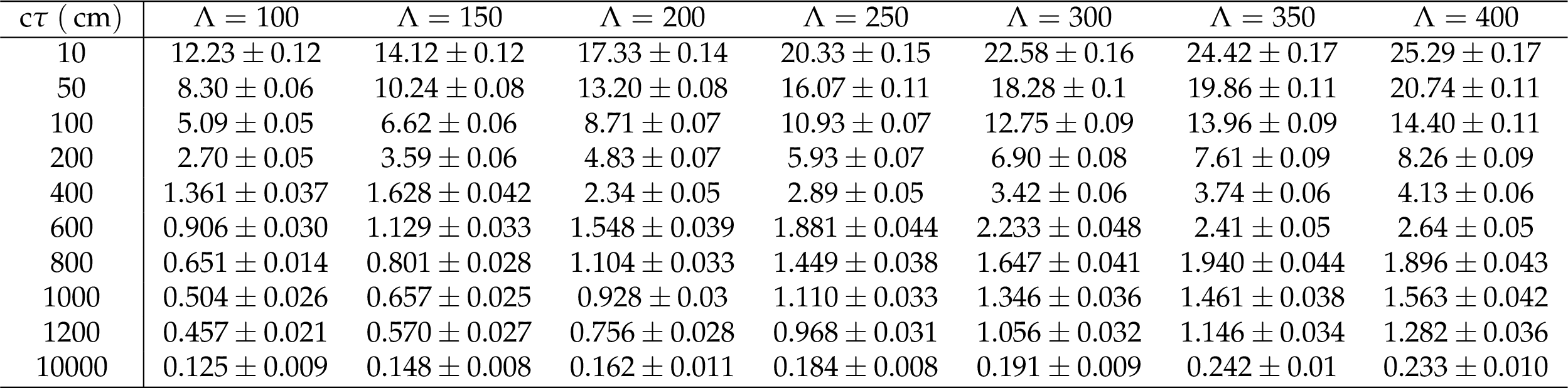
Additional Table 14:
(2017$\gamma $) Event selection efficiency times acceptance for the GMSB SPS8 grid points used in the analysis (unit of efficiency:%; unit of $\Lambda $: TeV) using the 2017$\gamma $ event selection. |
png pdf |
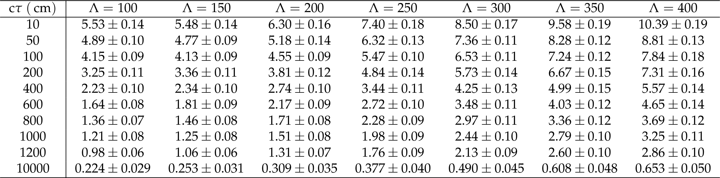
Additional Table 15:
(2017$\gamma \gamma $) Event selection efficiency times acceptance for the GMSB SPS8 grid points used in the analysis (unit of efficiency:%; unit of $\Lambda $: TeV) using the 2017$\gamma \gamma $ event selection. |
png pdf |
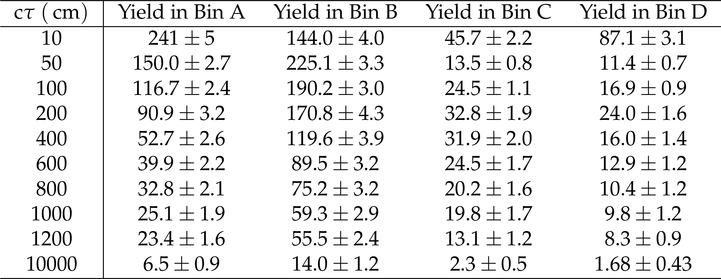
Additional Table 16:
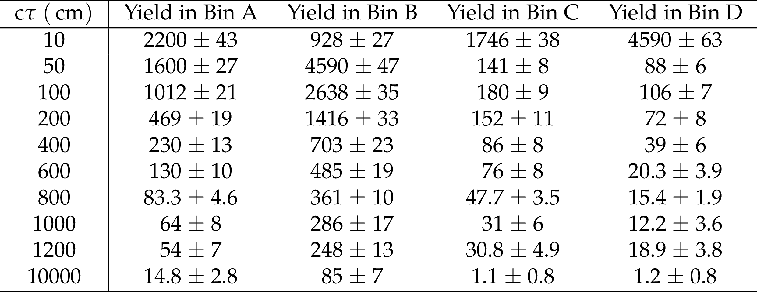
(2016) Event yields in bins A,B,C,D using the 2016 event selection for GMSB SPS8 $\Lambda = $ 100 TeV and varying c$\tau $. Please see the article for corresponding definitions of the $t_{\gamma}$-$ {{p_{\mathrm {T}}} ^\text {miss}}$ splits for each signal point. |
png pdf |
Additional Table 17:
(2016) Event yields in bins A,B,C,D using the 2016 event selection for GMSB SPS8 $\Lambda = $ 150 TeV and varying c$\tau $. Please see the article for corresponding definitions of the $t_{\gamma}$-$ {{p_{\mathrm {T}}} ^\text {miss}}$ splits for each signal point. |
png pdf |
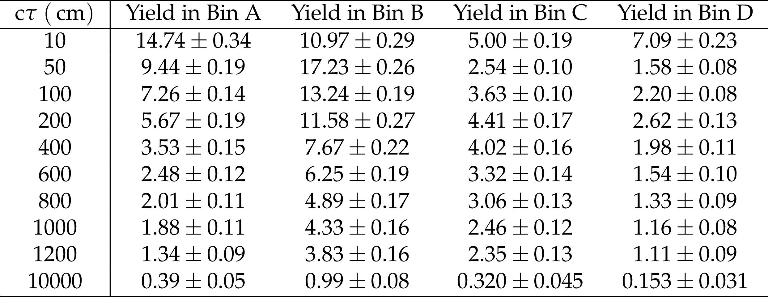
Additional Table 18:
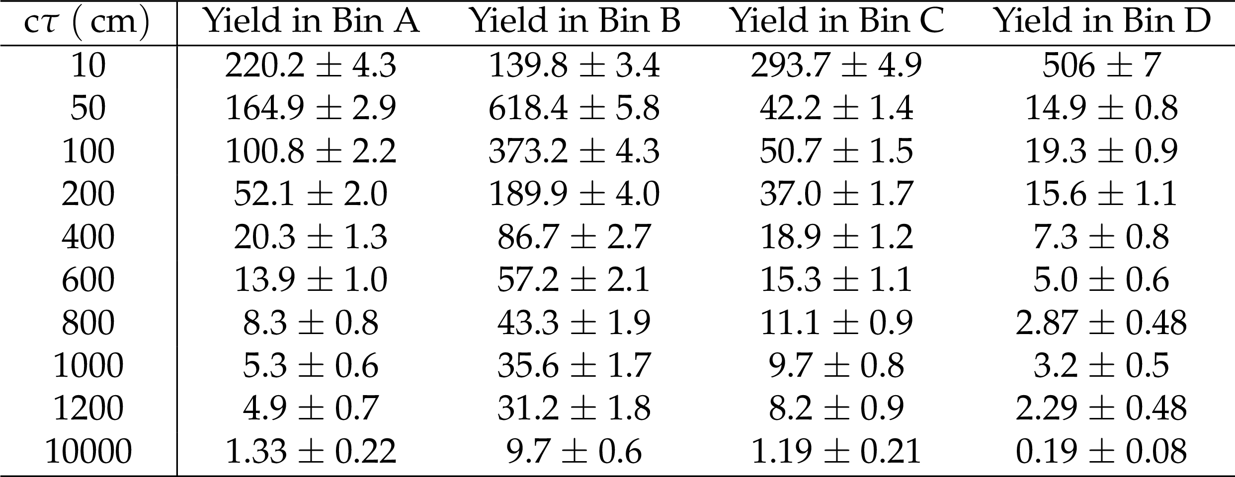
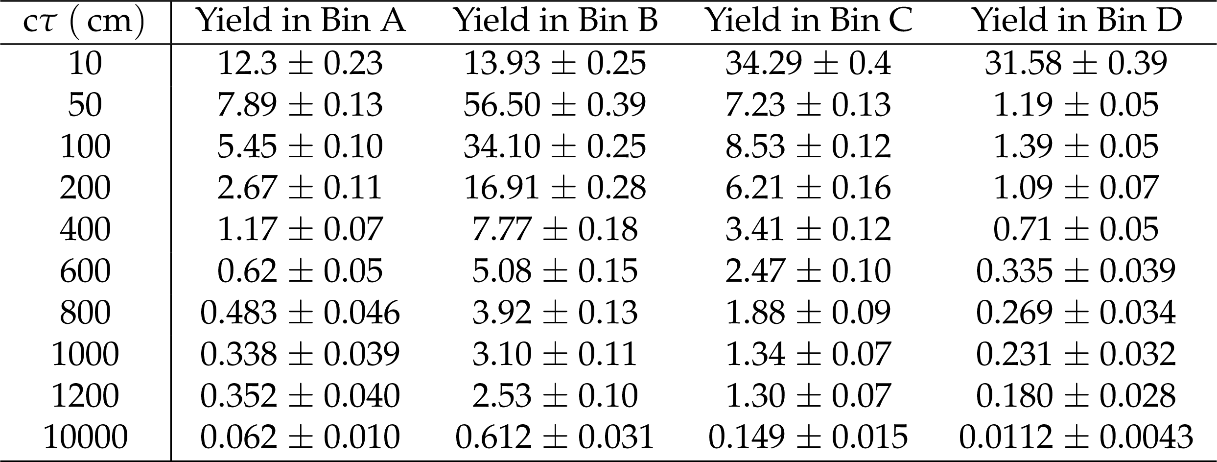
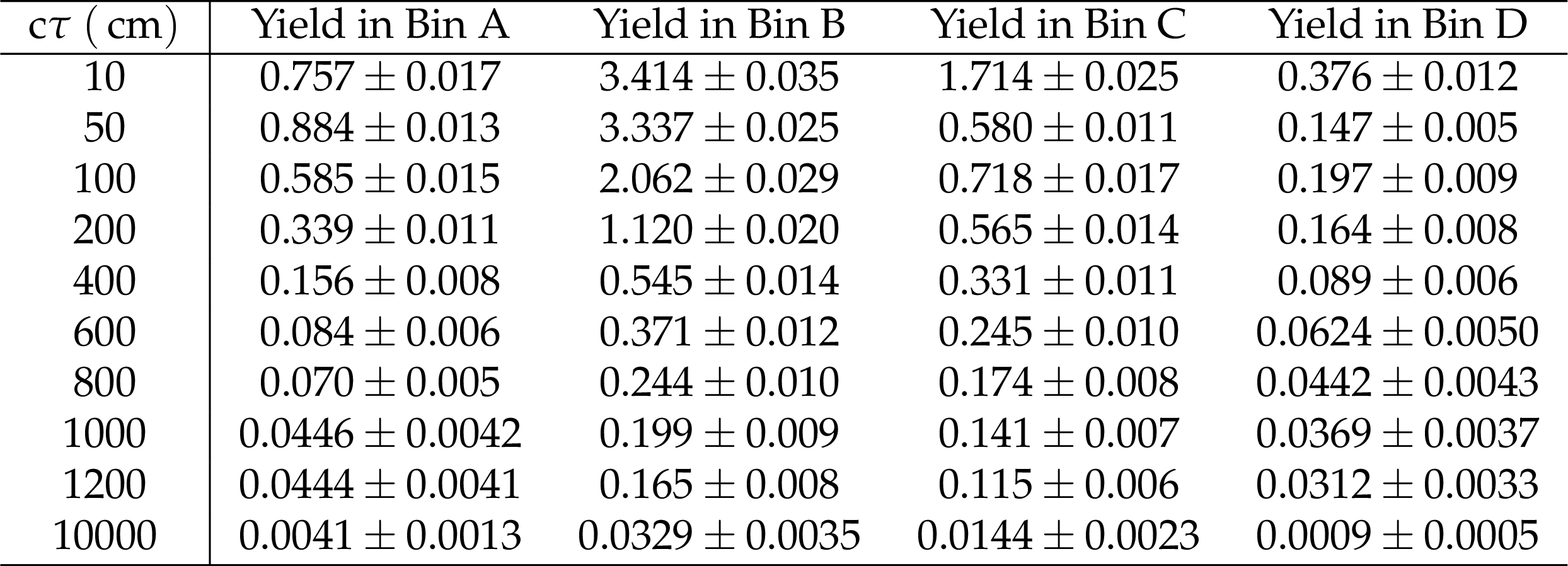
(2016) Event yields in bins A,B,C,D using the 2016 event selection for GMSB SPS8 $\Lambda = $ 200 TeV and varying c$\tau $. Please see the article for corresponding definitions of the $t_{\gamma}$-$ {{p_{\mathrm {T}}} ^\text {miss}}$ splits for each signal point. |
png pdf |
Additional Table 19:
(2016) Event yields in bins A,B,C,D using the 2016 event selection for GMSB SPS8 $\Lambda = $ 250 TeV and varying c$\tau $. Please see the article for corresponding definitions of the $t_{\gamma}$-$ {{p_{\mathrm {T}}} ^\text {miss}}$ splits for each signal point. |
png pdf |
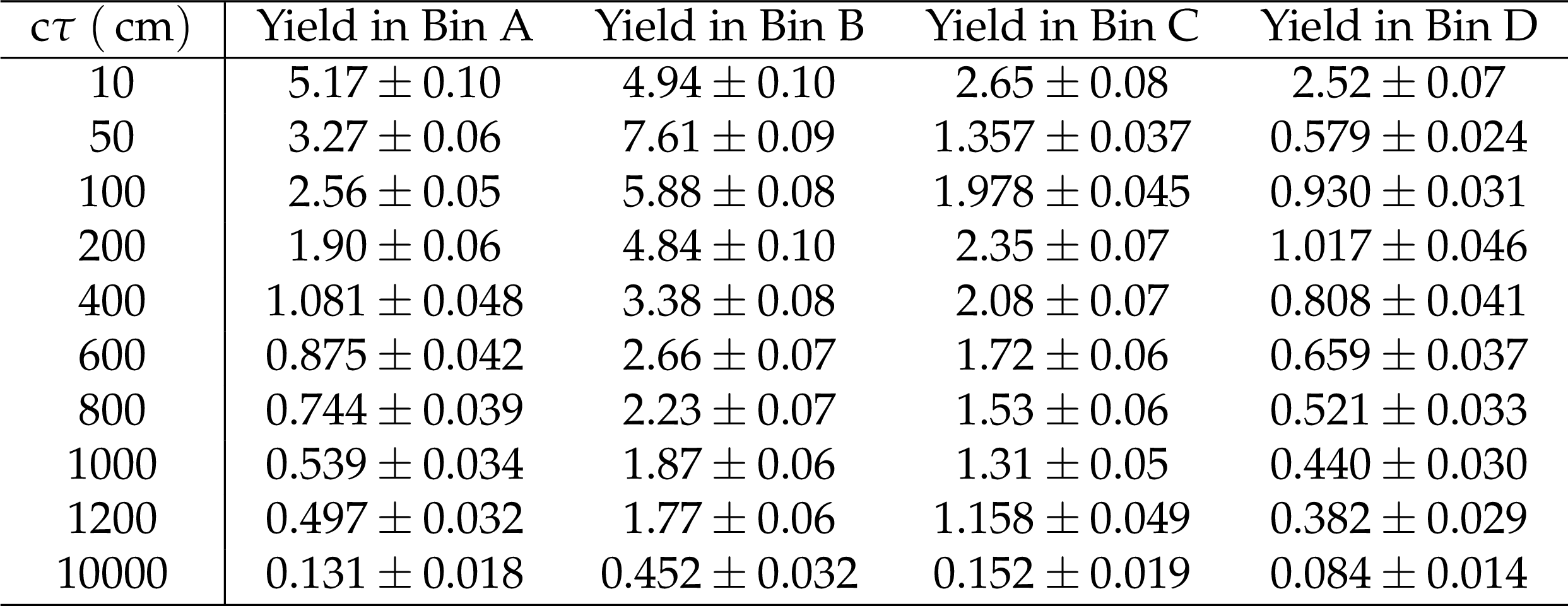
Additional Table 20:
(2016) Event yields in bins A,B,C,D using the 2016 event selection for GMSB SPS8 $\Lambda = $ 300 TeV and varying c$\tau $. Please see the article for corresponding definitions of the $t_{\gamma}$-$ {{p_{\mathrm {T}}} ^\text {miss}}$ splits for each signal point. |
png pdf |
Additional Table 21:
(2016) Event yields in bins A,B,C,D using the 2016 event selection for GMSB SPS8 $\Lambda = $ 350 TeV and varying c$\tau $. Please see the article for corresponding definitions of the $t_{\gamma}$-$ {{p_{\mathrm {T}}} ^\text {miss}}$ splits for each signal point. |
png pdf |
Additional Table 22:
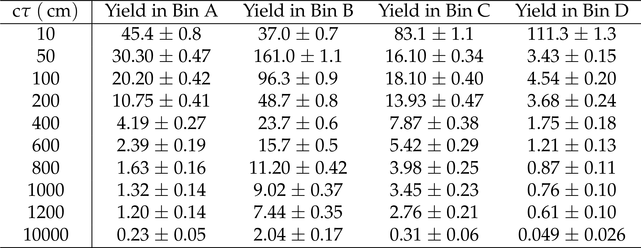
(2016) Event yields in bins A,B,C,D using the 2016 event selection for GMSB SPS8 $\Lambda = $ 400 TeV and varying c$\tau $. Please see the article for corresponding definitions of the $t_{\gamma}$-$ {{p_{\mathrm {T}}} ^\text {miss}}$ splits for each signal point. |

png pdf |
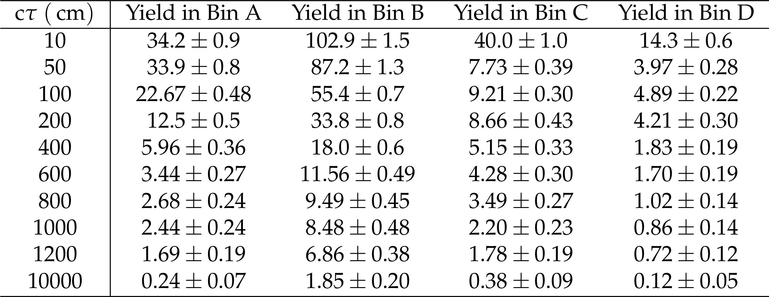
Additional Table 23:
(2017$\gamma $) Event yields in bins A,B,C,D using the 2017$\gamma $ event selection for GMSB SPS8 $\Lambda = $ 100 TeV and varying c$\tau $. Please see the article for corresponding definitions of the $t_{\gamma}$-$ {{p_{\mathrm {T}}} ^\text {miss}}$ splits for each signal point. |
png pdf |
Additional Table 24:
(2017$\gamma $) Event yields in bins A,B,C,D using the 2017$\gamma $ event selection for GMSB SPS8 $\Lambda = $ 150 TeV and varying c$\tau $. Please see the article for corresponding definitions of the $t_{\gamma}$-$ {{p_{\mathrm {T}}} ^\text {miss}}$ splits for each signal point. |

png pdf |
Additional Table 25:
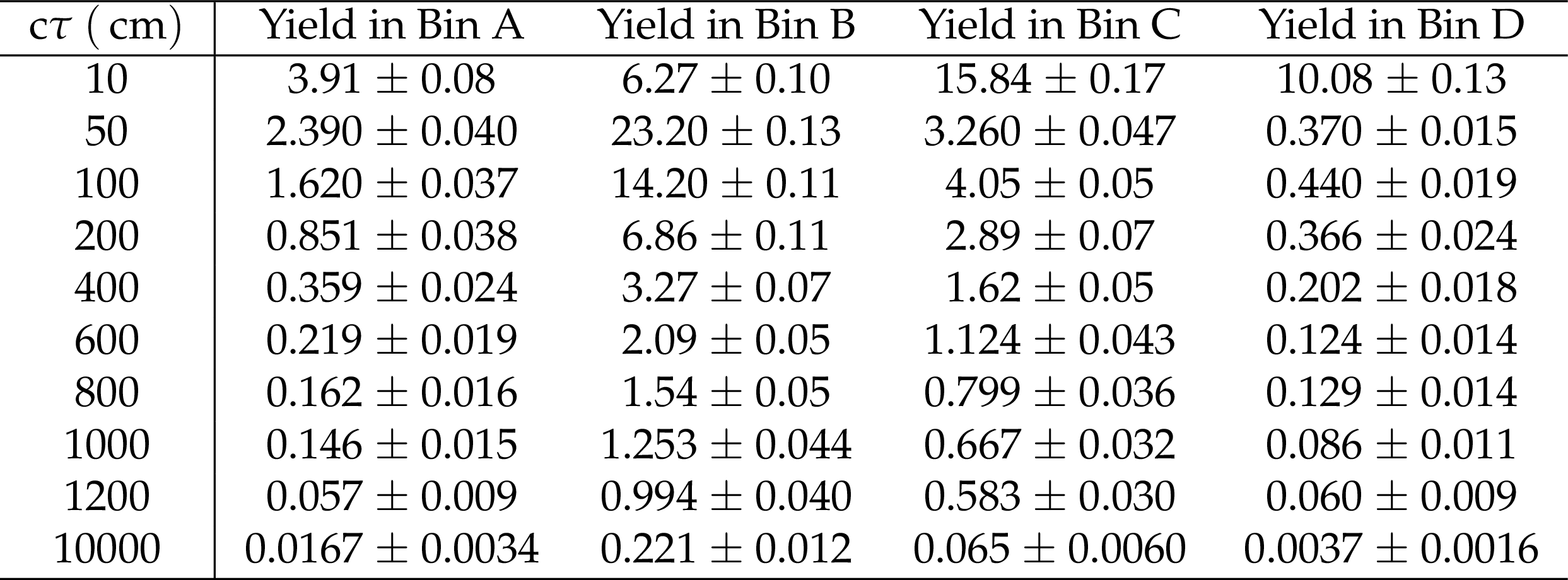
(2017$\gamma $) Event yields in bins A,B,C,D using the 2017$\gamma $ event selection for GMSB SPS8 $\Lambda = $ 200 TeV and varying c$\tau $. Please see the article for corresponding definitions of the $t_{\gamma}$-$ {{p_{\mathrm {T}}} ^\text {miss}}$ splits for each signal point. |
png pdf |
Additional Table 26:
(2017$\gamma $) Event yields in bins A,B,C,D using the 2017$\gamma $ event selection for GMSB SPS8 $\Lambda = $ 250 TeV and varying c$\tau $. Please see the article for corresponding definitions of the $t_{\gamma}$-$ {{p_{\mathrm {T}}} ^\text {miss}}$ splits for each signal point. |
png pdf |
Additional Table 27:
(2017$\gamma $) Event yields in bins A,B,C,D using the 2017$\gamma $ event selection for GMSB SPS8 $\Lambda = $ 300 TeV and varying c$\tau $. Please see the article for corresponding definitions of the $t_{\gamma}$-$ {{p_{\mathrm {T}}} ^\text {miss}}$ splits for each signal point. |

png pdf |
Additional Table 28:
(2017$\gamma $) Event yields in bins A,B,C,D using the 2017$\gamma $ event selection for GMSB SPS8 $\Lambda = $ 350 TeV and varying c$\tau $. Please see the article for corresponding definitions of the $t_{\gamma}$-$ {{p_{\mathrm {T}}} ^\text {miss}}$ splits for each signal point. |

png pdf |
Additional Table 29:
(2017$\gamma $) Event yields in bins A,B,C,D using the 2017$\gamma $ event selection for GMSB SPS8 $\Lambda = $ 400 TeV and varying c$\tau $. Please see the article for corresponding definitions of the $t_{\gamma}$-$ {{p_{\mathrm {T}}} ^\text {miss}}$ splits for each signal point. |

png pdf |
Additional Table 30:
(2017$\gamma \gamma $) Event yields in bins A,B,C,D using the 2017$\gamma \gamma $ event selection for GMSB SPS8 $\Lambda = $ 100 TeV and varying c$\tau $. Please see the article for corresponding definitions of the $t_{\gamma}$-$ {{p_{\mathrm {T}}} ^\text {miss}}$ splits for each signal point. |

png pdf |
Additional Table 31:
(2017$\gamma \gamma $) Event yields in bins A,B,C,D using the 2017$\gamma \gamma $ event selection for GMSB SPS8 $\Lambda = $ 150 TeV and varying c$\tau $. Please see the article for corresponding definitions of the $t_{\gamma}$-$ {{p_{\mathrm {T}}} ^\text {miss}}$ splits for each signal point. |
png pdf |
Additional Table 32:
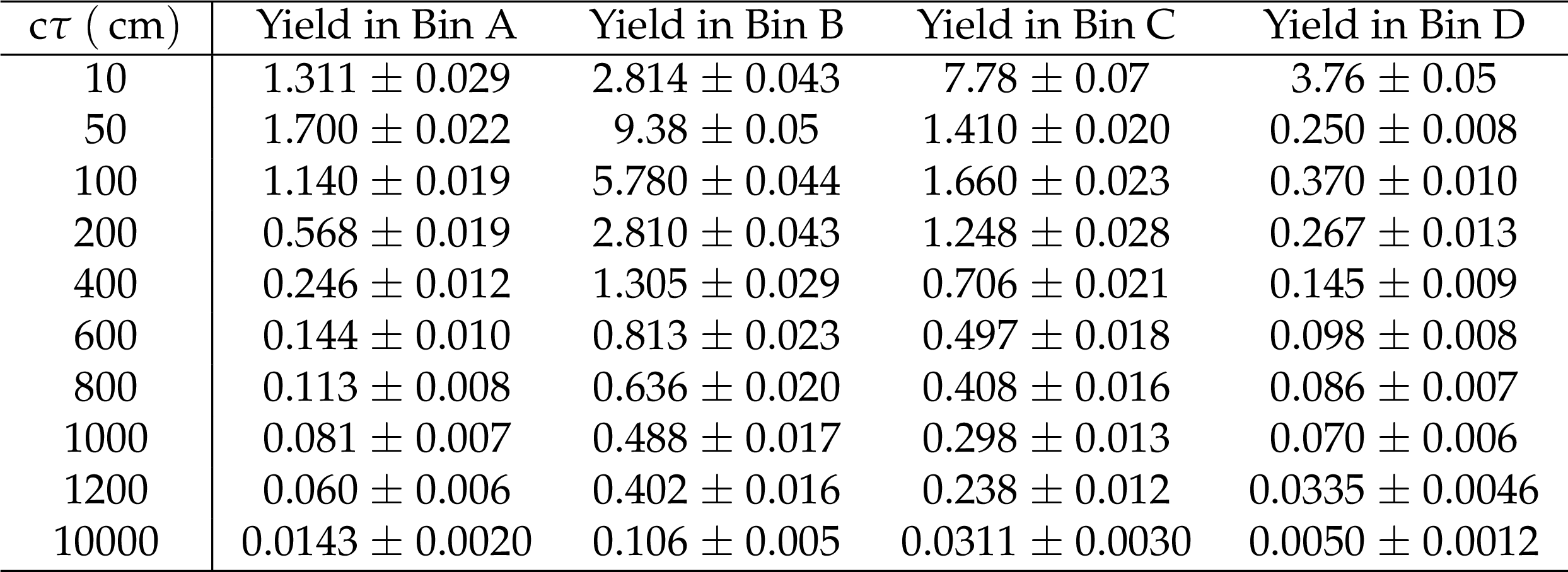
(2017$\gamma \gamma $) Event yields in bins A,B,C,D using the 2017$\gamma \gamma $ event selection for GMSB SPS8 $\Lambda = $ 200 TeV and varying c$\tau $. Please see the article for corresponding definitions of the $t_{\gamma}$-$ {{p_{\mathrm {T}}} ^\text {miss}}$ splits for each signal point. |

png pdf |
Additional Table 33:
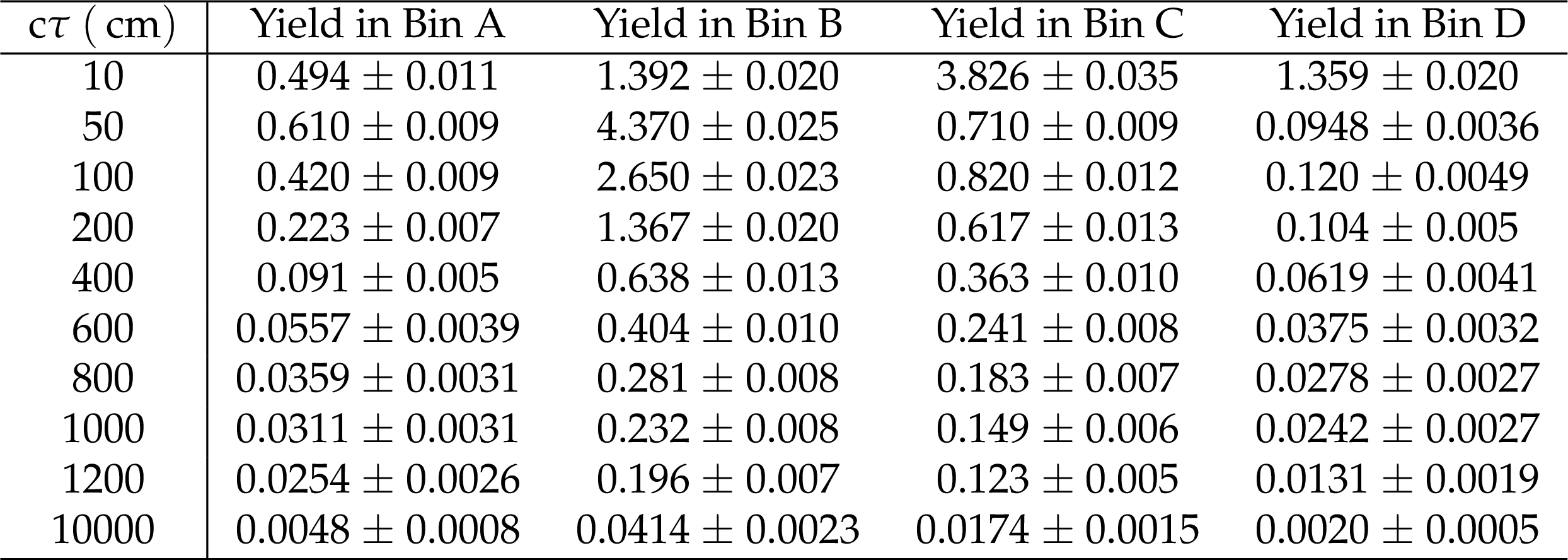
(2017$\gamma \gamma $) Event yields in bins A,B,C,D using the 2017$\gamma \gamma $ event selection for GMSB SPS8 $\Lambda = $ 250 TeV and varying c$\tau $. Please see the article for corresponding definitions of the $t_{\gamma}$-$ {{p_{\mathrm {T}}} ^\text {miss}}$ splits for each signal point. |

png pdf |
Additional Table 34:
(2017$\gamma \gamma $) Event yields in bins A,B,C,D using the 2017$\gamma \gamma $ event selection for GMSB SPS8 $\Lambda = $ 300 TeV and varying c$\tau $. Please see the article for corresponding definitions of the $t_{\gamma}$-$ {{p_{\mathrm {T}}} ^\text {miss}}$ splits for each signal point. |

png pdf |
Additional Table 35:
(2017$\gamma \gamma $) Event yields in bins A,B,C,D using the 2017$\gamma \gamma $ event selection for GMSB SPS8 $\Lambda = $ 350 TeV and varying c$\tau $. Please see the article for corresponding definitions of the $t_{\gamma}$-$ {{p_{\mathrm {T}}} ^\text {miss}}$ splits for each signal point. |
png pdf |
Additional Table 36:
(2017$\gamma \gamma $) Event yields in bins A,B,C,D using the 2017$\gamma \gamma $ event selection for GMSB SPS8 $\Lambda = $ 400 TeV and varying c$\tau $. Please see the article for corresponding definitions of the $t_{\gamma}$-$ {{p_{\mathrm {T}}} ^\text {miss}}$ splits for each signal point. |
| References | ||||
| 1 | P. Ramond | Dual theory for free fermions | PRD 3 (1971) 2415 | |
| 2 | P. Ramond | An interpretation of dual theories | Nuovo Cim. A 4 (1971) 544 | |
| 3 | \relax Yu. A. Golfand and E. P. Likhtman | Extension of the algebra of Poincaré group generators and violation of P invariance | JEPTL 13 (1971) 323 | |
| 4 | D. V. Volkov and V. P. Akulov | Possible universal neutrino interaction | JEPTL 16 (1972) 438 | |
| 5 | J. Wess and B. Zumino | Supergauge transformations in four-dimensions | NPB 70 (1974) 39 | |
| 6 | D. Z. Freedman, P. van Nieuwenhuizen, and S. Ferrara | Progress toward a theory of supergravity | PRD 13 (1976) 3214 | |
| 7 | S. Deser and B. Zumino | Consistent supergravity | PLB 62 (1976) 335 | |
| 8 | D. Z. Freedman and P. van Nieuwenhuizen | Properties of supergravity theory | PRD 14 (1976) 912 | |
| 9 | S. Ferrara and P. van Nieuwenhuizen | Consistent supergravity with complex spin 3/2 gauge fields | PRL 37 (1976) 1669 | |
| 10 | P. Fayet | Supergauge invariant extension of the Higgs mechanism and a model for the electron and its neutrino | NPB 90 (1975) 104 | |
| 11 | A. H. Chamseddine, R. L. Arnowitt, and P. Nath | Locally supersymmetric grand unification | PRL 49 (1982) 970 | |
| 12 | R. Barbieri, S. Ferrara, and C. A. Savoy | Gauge models with spontaneously broken local supersymmetry | PLB 119 (1982) 343 | |
| 13 | L. J. Hall, J. D. Lykken, and S. Weinberg | Supergravity as the messenger of supersymmetry breaking | PRD 27 (1983) 2359 | |
| 14 | G. L. Kane, C. F. Kolda, L. Roszkowski, and J. D. Wells | Study of constrained minimal supersymmetry | PRD 49 (1994) 6173 | hep-ph/9312272 |
| 15 | G. F. Giudice and R. Rattazzi | Theories with gauge mediated supersymmetry breaking | PR 322 (1999) 419 | hep-ph/9801271 |
| 16 | S. Dimopoulos, M. Dine, S. Raby, and S. D. Thomas | Experimental signatures of low-energy gauge mediated supersymmetry breaking | PRL 76 (1996) 3494 | hep-ph/9601367 |
| 17 | P. Fayet | Mixing between gravitational and weak interactions through the massive gravitino | PLB 70 (1977) 461 | |
| 18 | H. Baer, M. Brhlik, C. H. Chen, and X. Tata | Signals for the minimal gauge-mediated supersymmetry breaking model at the Fermilab Tevatron collider | PRD 55 (1997) 4463 | hep-ph/9610358 |
| 19 | H. Baer, P. G. Mercadante, X. Tata, and Y. L. Wang | Reach of Tevatron upgrades in gauge-mediated supersymmetry breaking models | PRD 60 (1999) 055001 | hep-ph/9903333 |
| 20 | S. Dimopoulos, S. Thomas, and J. D. Wells | Sparticle spectroscopy and electroweak symmetry breaking with gauge-mediated supersymmetry breaking | NPB 488 (1997) 39 | hep-ph/9609434 |
| 21 | J. R. Ellis, J. L. Lopez, and D. V. Nanopoulos | Analysis of LEP constraints on supersymmetric models with a light gravitino | PLB 394 (1997) 354 | hep-ph/9610470 |
| 22 | M. Dine, A. E. Nelson, Y. Nir, and Y. Shirman | New tools for low energy dynamical supersymmetry breaking | PRD 53 (1996) 2658 | hep-ph/9507378 |
| 23 | G. F. Giudice and R. Rattazzi | Gauge-mediated supersymmetry breaking | in Perspectives on supersymmetry, p. 355 World Scientific, Singapore | |
| 24 | B. C. Allanach et al. | The Snowmass points and slopes: Benchmarks for SUSY searches | EPJC 25 (2002) 113 | hep-ph/0202233 |
| 25 | C. H. Chen and J. F. Gunion | Maximizing hadron collider sensitivity to gauge mediated supersymmetry breaking models | PLB 420 (1998) 77 | hep-ph/9707302 |
| 26 | CMS Collaboration | Search for long-lived particles decaying to photons and missing energy in proton-proton collisions at $ \sqrt{s}= $ 7 TeV | PLB 722 (2013) 273 | CMS-EXO-11-035 1212.1838 |
| 27 | ATLAS Collaboration | Search for nonpointing and delayed photons in the diphoton and missing transverse momentum final state in 8 TeV pp collisions at the LHC using the ATLAS detector | PRD 90 (2014) 112005 | 1409.5542 |
| 28 | CMS Collaboration | The CMS experiment at the CERN LHC | JINST 3 (2008) S08004 | CMS-00-001 |
| 29 | CMS Collaboration | The CMS trigger system | JINST 12 (2017) P01020 | CMS-TRG-12-001 1609.02366 |
| 30 | J. Alwall et al. | Comparative study of various algorithms for the merging of parton showers and matrix elements in hadronic collisions | EPJC 53 (2008) 473 | 0706.2569 |
| 31 | T. Gleisberg et al. | Event generation with SHERPA 1.1 | JHEP 02 (2009) 007 | 0811.4622 |
| 32 | T. Sjostrand, S. Mrenna, and P. Skands | A brief introduction to PYTHIA 8.1 | Comp. Phys. Commun. 178 (2008) 852 | |
| 33 | P. Skands, S. Carrazza, and J. Rojo | Tuning PYTHIA 8.1: the Monash 2013 tune | EPJC 74 (2014) 3024 | |
| 34 | CMS Collaboration | Extraction and validation of a new set of CMS PYTHIA8 tunes from underlying-event measurements | CMS-PAS-GEN-17-001 | CMS-PAS-GEN-17-001 |
| 35 | NNPDF Collaboration | Parton distributions for the LHC Run II | JHEP 04 (2015) 040 | 1410.8849 |
| 36 | NNPDF Collaboration | Parton distributions from high-precision collider data | EPJC 77 (2017) 663 | 1706.00428 |
| 37 | GEANT4 Collaboration | GEANT4---a simulation toolkit | NIMA 506 (2003) 250 | |
| 38 | CMS Collaboration | Particle-flow reconstruction and global event description with the CMS detector | JINST 12 (2017) P10003 | CMS-PRF-14-001 1706.04965 |
| 39 | CMS Collaboration | Performance of photon reconstruction and identification with the CMS detector in proton-proton collisions at $ \sqrt{s} = $ 8 TeV | JINST 10 (2015) P08010 | CMS-EGM-14-001 1502.02702 |
| 40 | M. Cacciari, G. P. Salam, and G. Soyez | The anti-$ {k_{\mathrm{T}}} $ jet clustering algorithm | JHEP 04 (2008) 063 | 0802.1189 |
| 41 | M. Cacciari, G. P. Salam, and G. Soyez | FastJet user manual | EPJC 72 (2012) 1896 | 1111.6097 |
| 42 | CMS Collaboration | Jet algorithms performance in 13 TeV data | CMS-PAS-JME-16-003 | CMS-PAS-JME-16-003 |
| 43 | CMS Collaboration | Performance of missing transverse momentum in pp collisions at $ \sqrt{s}= $ 13 TeV using the CMS detector | CMS-PAS-JME-17-001 | CMS-PAS-JME-17-001 |
| 44 | CMS Collaboration | Performance of missing transverse momentum reconstruction in proton-proton collisions at $ \sqrt{s} = $ 13 TeV using the CMS detector | JINST 14 (2019), no. 07, P07004 | CMS-JME-17-001 1903.06078 |
| 45 | CMS Collaboration | Time Reconstruction and Performance of the CMS Electromagnetic Calorimeter | JINST 5 (2010) T03011 | CMS-CFT-09-006 0911.4044 |
| 46 | D. del Re | Timing performance of the CMS ECAL and prospects for the future | J. Phys. Conf. Ser. 587 (2015), no. 1, 012003 | |
| 47 | CMS Collaboration | CMS Luminosity Measurements for the 2016 Data Taking Period | CMS-PAS-LUM-17-001 | CMS-PAS-LUM-17-001 |
| 48 | CMS Collaboration | CMS luminosity measurement for the 2017 data-taking period at $ \sqrt{s} = $ 13 TeV | CMS-PAS-LUM-17-004 | CMS-PAS-LUM-17-004 |
| 49 | A. L. Read | Presentation of search results: The $ CL_{s} $ technique | JPG 28 (2002) 2693 | |
| 50 | T. Junk | Confidence level computation for combining searches with small statistics | NIMA 434 (1999) 435 | hep-ex/9902006 |
| 51 | ATLAS and CMS Collaborations | Procedure for the LHC Higgs boson search combination in summer 2011 | CMS-NOTE-2011-005 | |
|
|
Compact Muon Solenoid LHC, CERN |
|

|

|

|

|

|