

Compact Muon Solenoid
LHC, CERN
| CMS-PAS-BPH-15-009 | ||
| Angular analysis of the decay ${\mathrm B^{+} \to \mathrm K^{*+} \mu^{+} \mu^{-}}$ in proton-proton collisions at $\sqrt{s}= $ 8 TeV | ||
| CMS Collaboration | ||
| July 2020 | ||
| Abstract: Angular distributions of the decay ${\mathrm B^{+} \to \mathrm K^{*+} \mu^{+} \mu^{-}}$ are studied using events collected with the CMS detector from $\sqrt{s}= $ 8 TeV proton-proton collisions, corresponding to an integrated luminosity of 20.0 fb$^{-1}$. The forward-backward asymmetry of the muons and the longitudinal polarization of the $\mathrm K^{*+}$ meson are determined for an integrated sample and as a function of the dimuon invariant mass squared. These are the first results from this exclusive decay mode and are in agreement with standard model predictions. | ||
|
Links:
CDS record (PDF) ;
CADI line (restricted) ;
These preliminary results are superseded in this paper, JHEP 04 (2021) 124. The superseded preliminary plots can be found here. |
||
| Figures | |

png pdf |
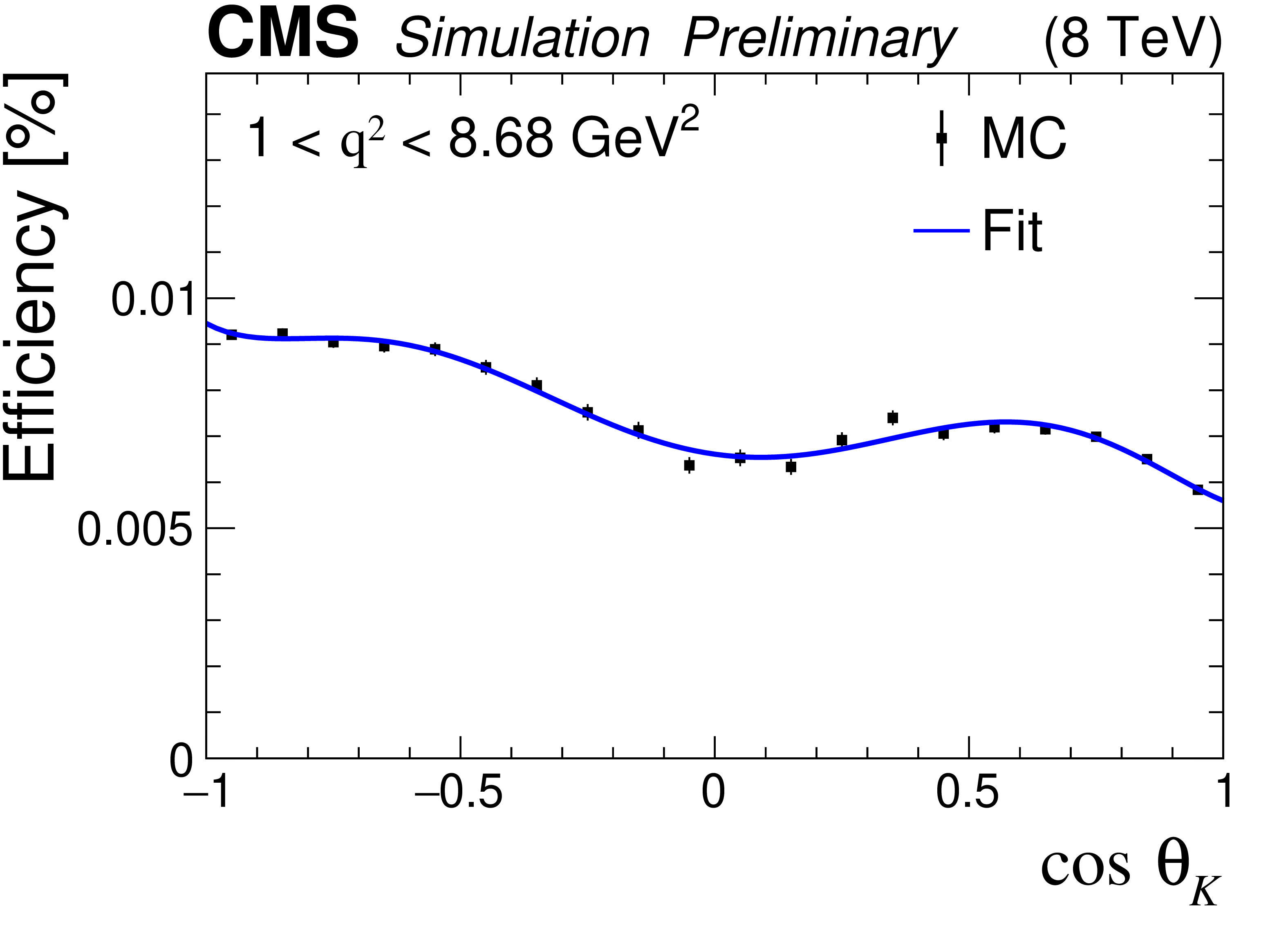
Figure 1:
The signal efficiency as a function $\cos\theta _{\mathrm{K}} $ for different ${q^2}$ ranges. The vertical bars indicate the statistical uncertainty. The curves show the fitted result, as described in the text. |
png pdf |
Figure 1-a:
The signal efficiency as a function $\cos\theta _{\mathrm{K}} $ for different ${q^2}$ ranges. The vertical bars indicate the statistical uncertainty. The curves show the fitted result, as described in the text. |
png pdf |
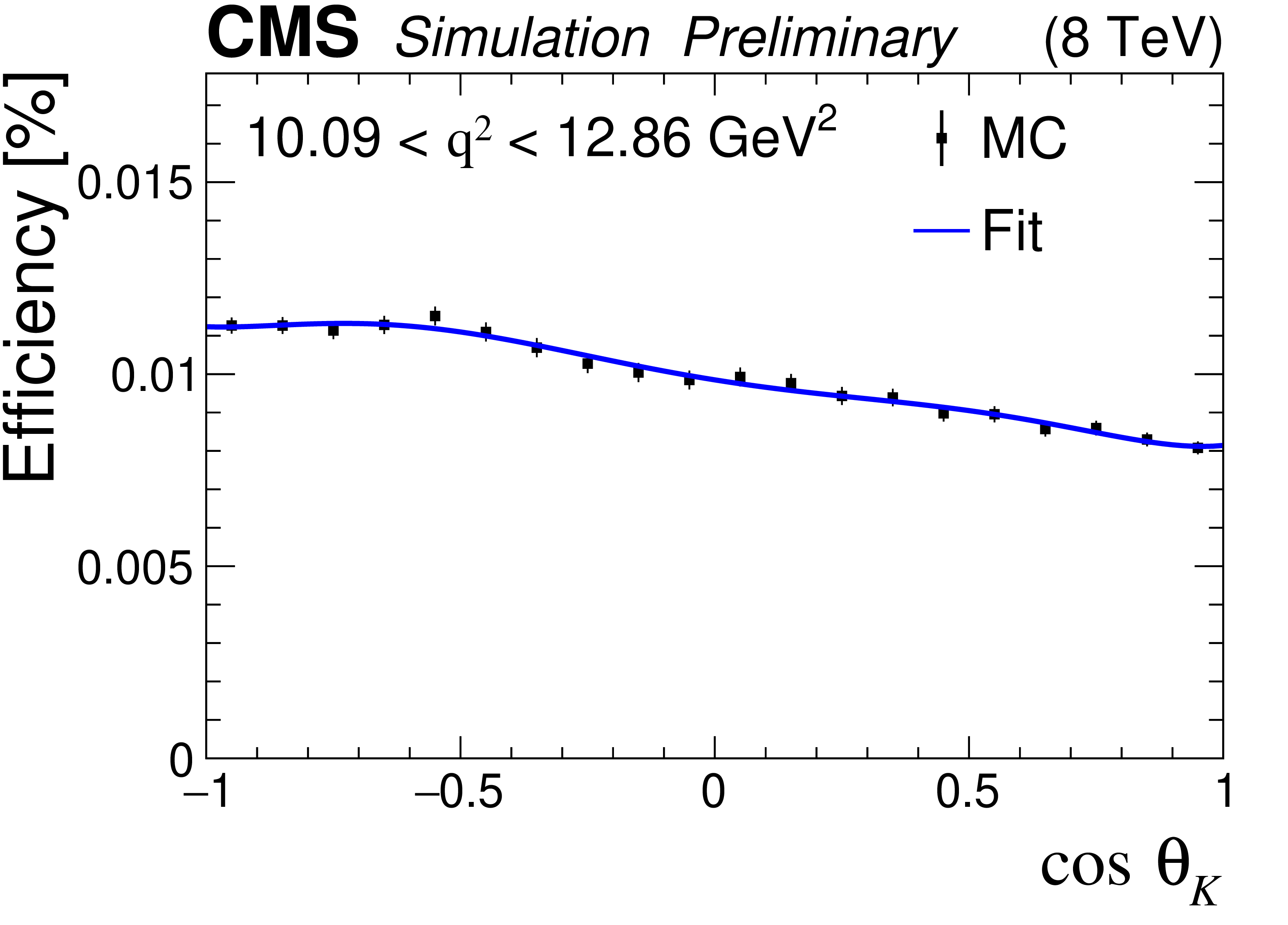
Figure 1-b:
The signal efficiency as a function $\cos\theta _{\mathrm{K}} $ for different ${q^2}$ ranges. The vertical bars indicate the statistical uncertainty. The curves show the fitted result, as described in the text. |
png pdf |
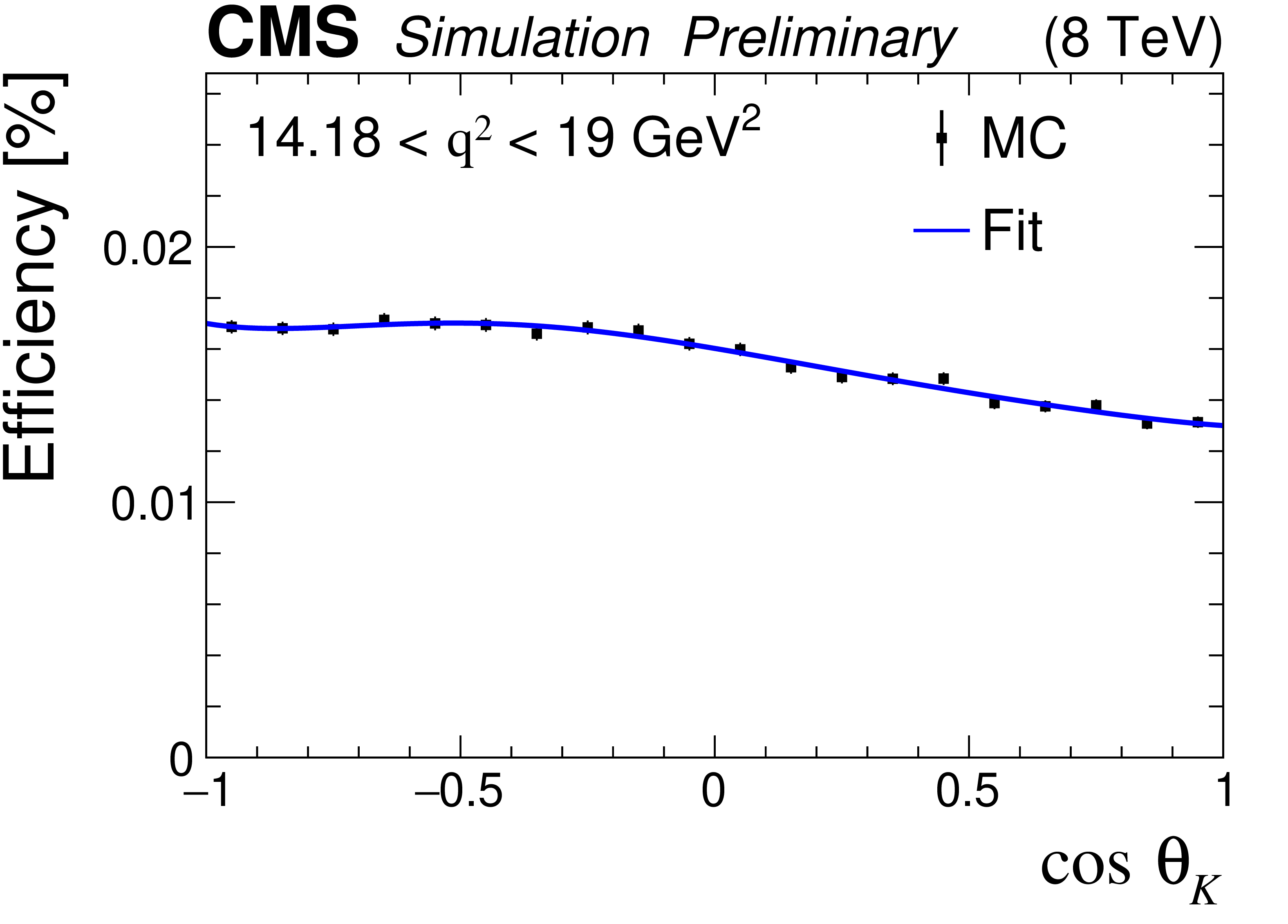
Figure 1-c:
The signal efficiency as a function $\cos\theta _{\mathrm{K}} $ for different ${q^2}$ ranges. The vertical bars indicate the statistical uncertainty. The curves show the fitted result, as described in the text. |
png pdf |
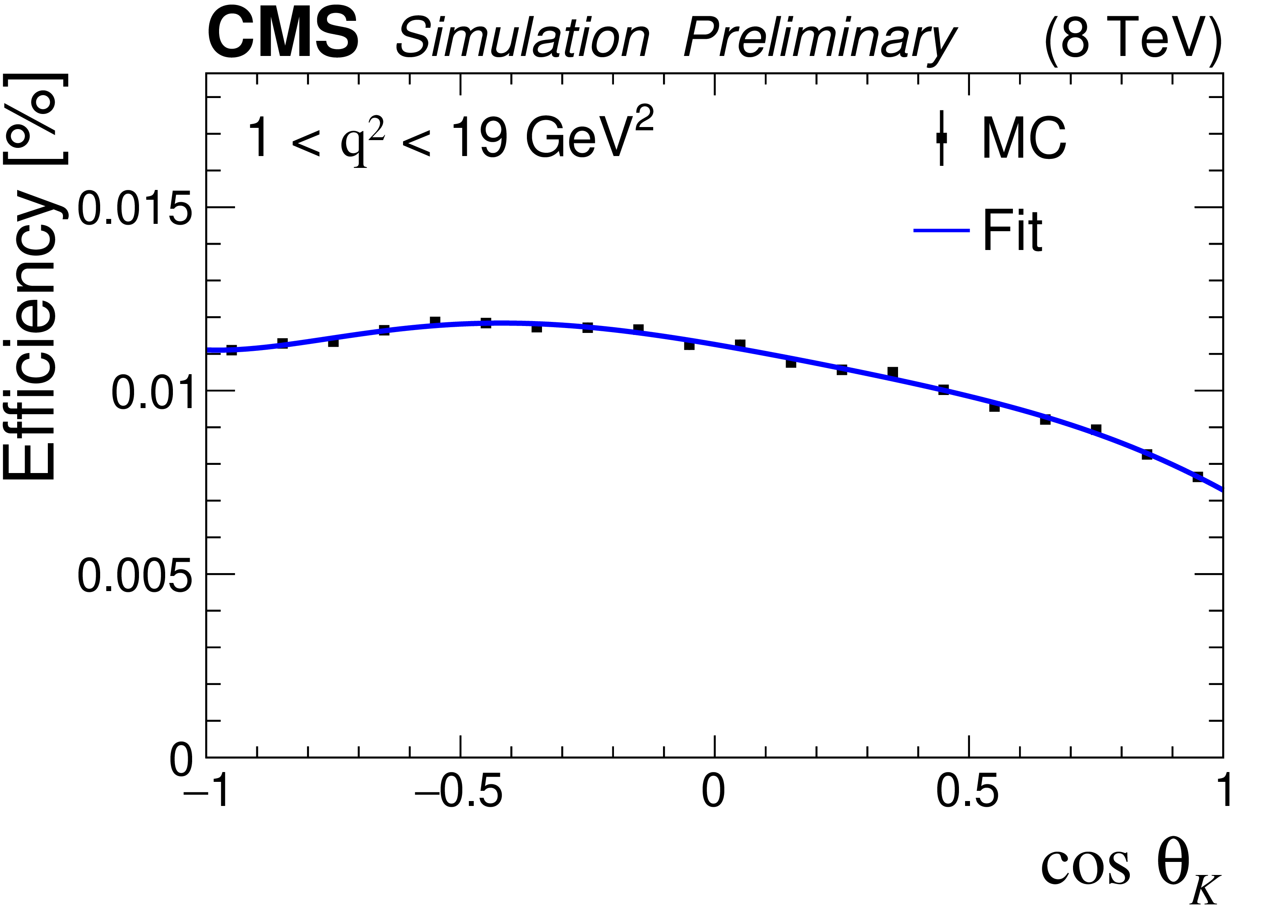
Figure 1-d:
The signal efficiency as a function $\cos\theta _{\mathrm{K}} $ for different ${q^2}$ ranges. The vertical bars indicate the statistical uncertainty. The curves show the fitted result, as described in the text. |
png pdf |
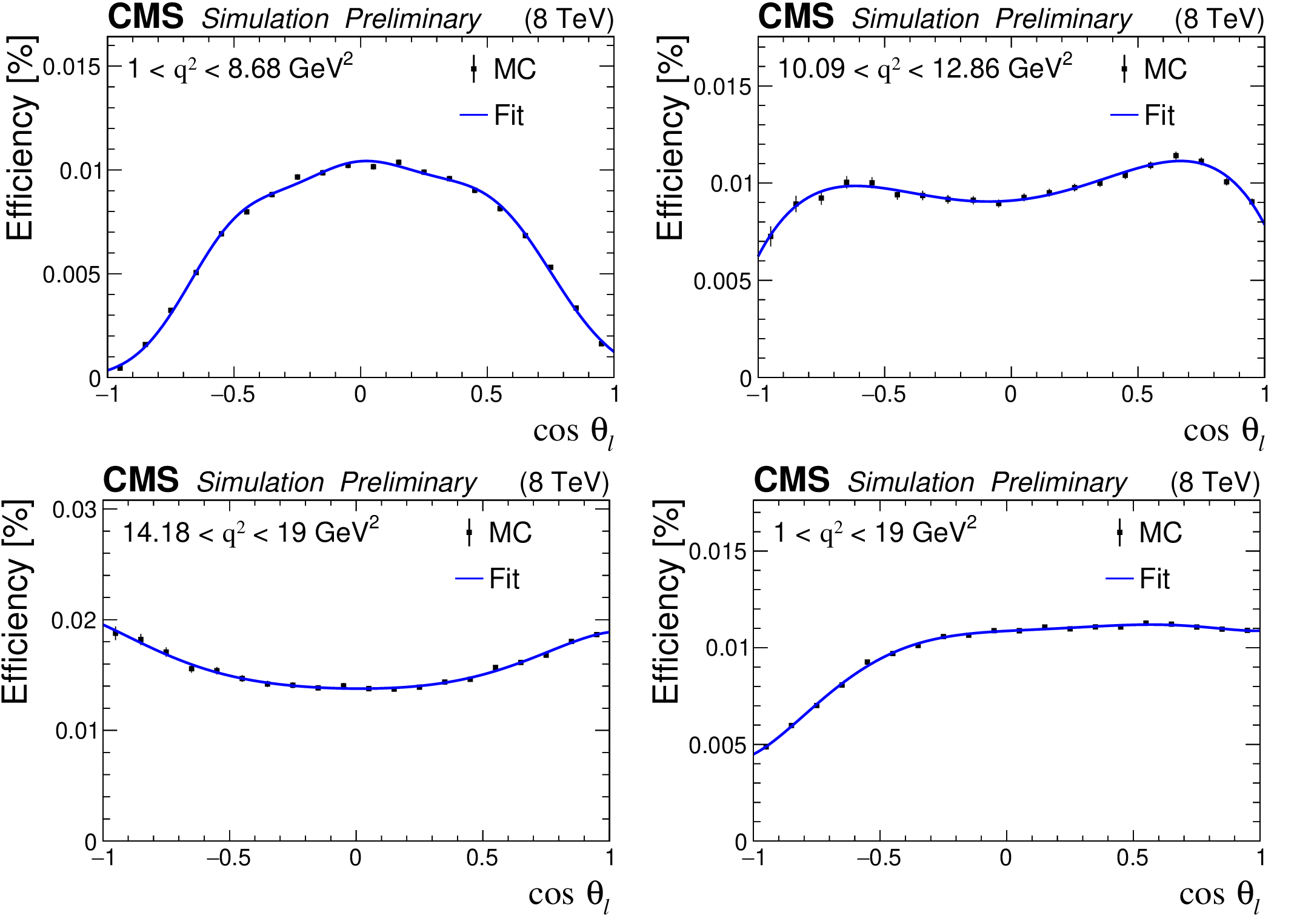
Figure 2:
The signal efficiency as a function $\cos\theta _{\ell} $ for different ${q^2}$ ranges. The vertical bars indicate the statistical uncertainty. The curves show the fitted result, as described in the text. |

png pdf |
Figure 2-a:
The signal efficiency as a function $\cos\theta _{\ell} $ for different ${q^2}$ ranges. The vertical bars indicate the statistical uncertainty. The curves show the fitted result, as described in the text. |
png pdf |
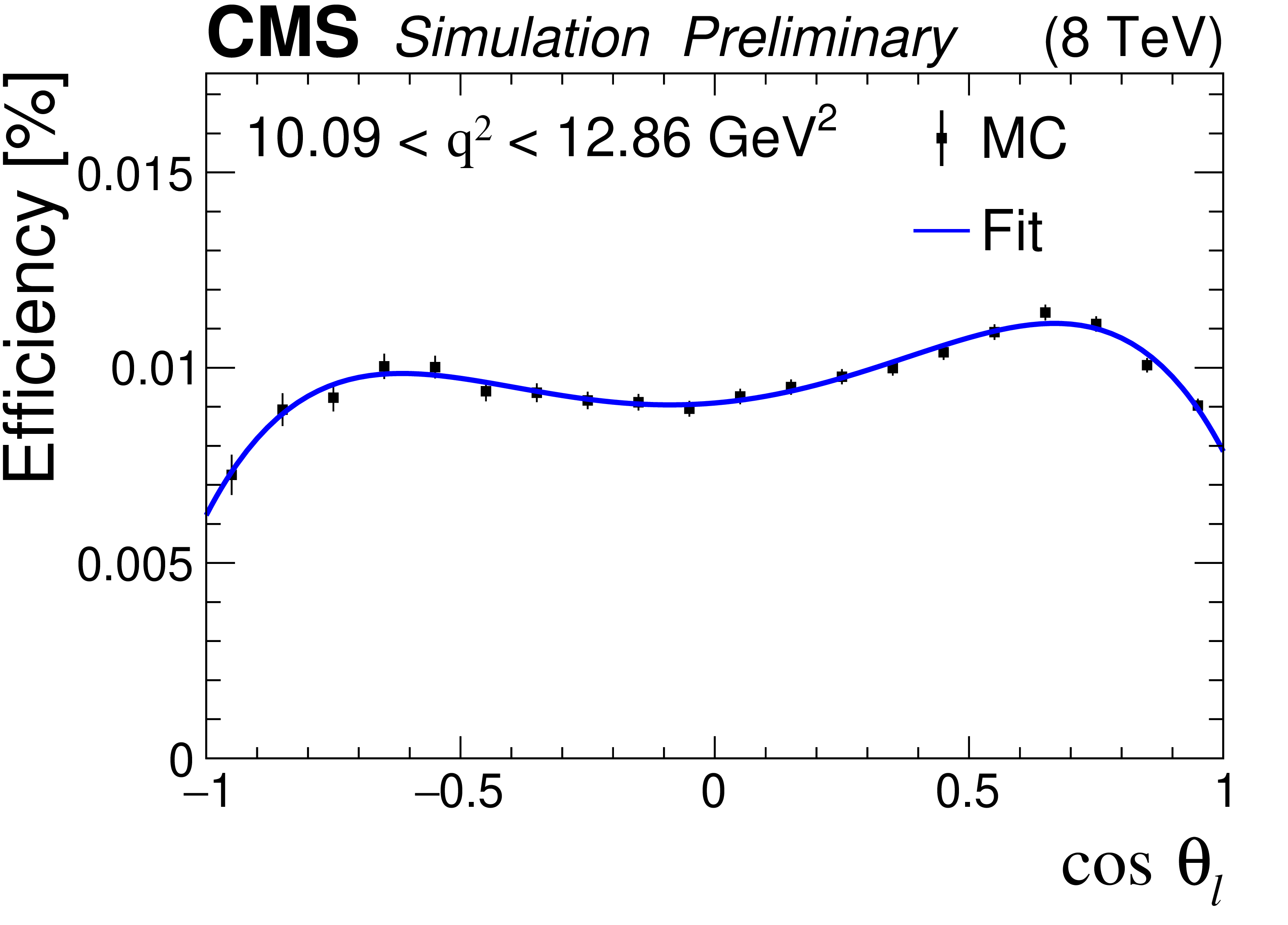
Figure 2-b:
The signal efficiency as a function $\cos\theta _{\ell} $ for different ${q^2}$ ranges. The vertical bars indicate the statistical uncertainty. The curves show the fitted result, as described in the text. |
png pdf |
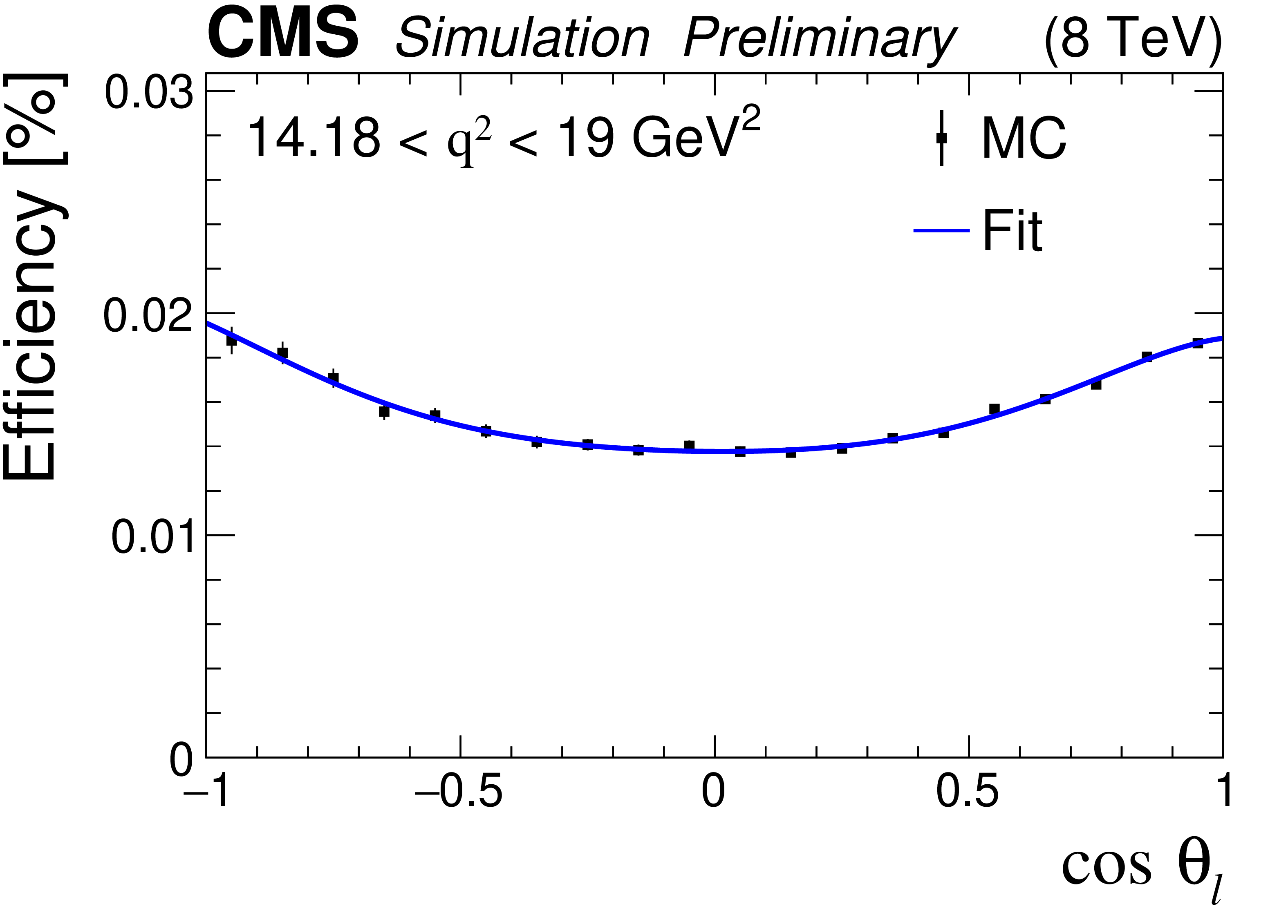
Figure 2-c:
The signal efficiency as a function $\cos\theta _{\ell} $ for different ${q^2}$ ranges. The vertical bars indicate the statistical uncertainty. The curves show the fitted result, as described in the text. |
png pdf |
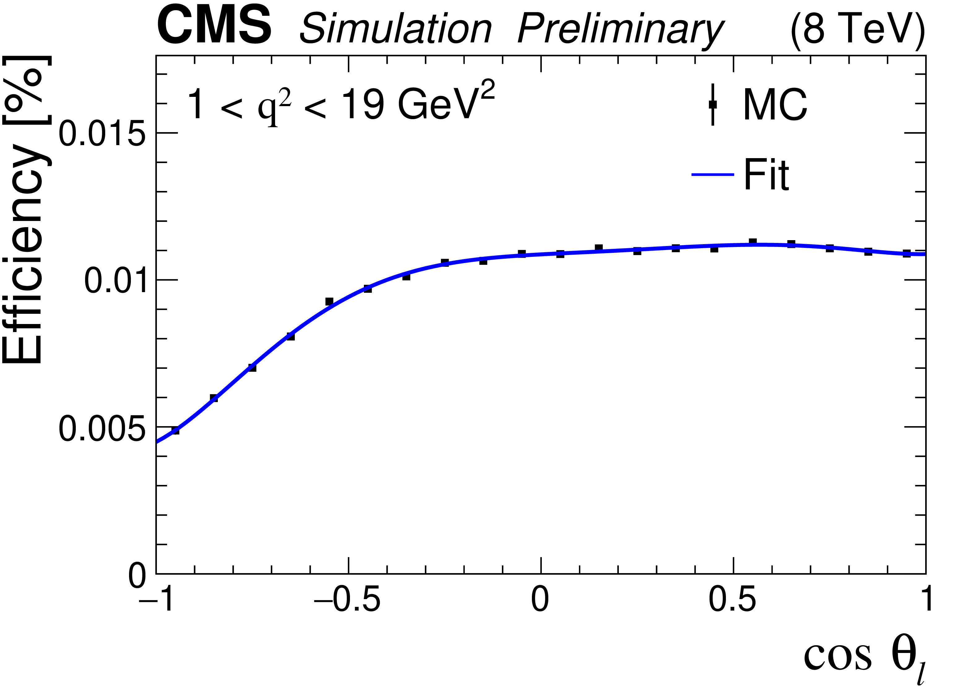
Figure 2-d:
The signal efficiency as a function $\cos\theta _{\ell} $ for different ${q^2}$ ranges. The vertical bars indicate the statistical uncertainty. The curves show the fitted result, as described in the text. |
png pdf |
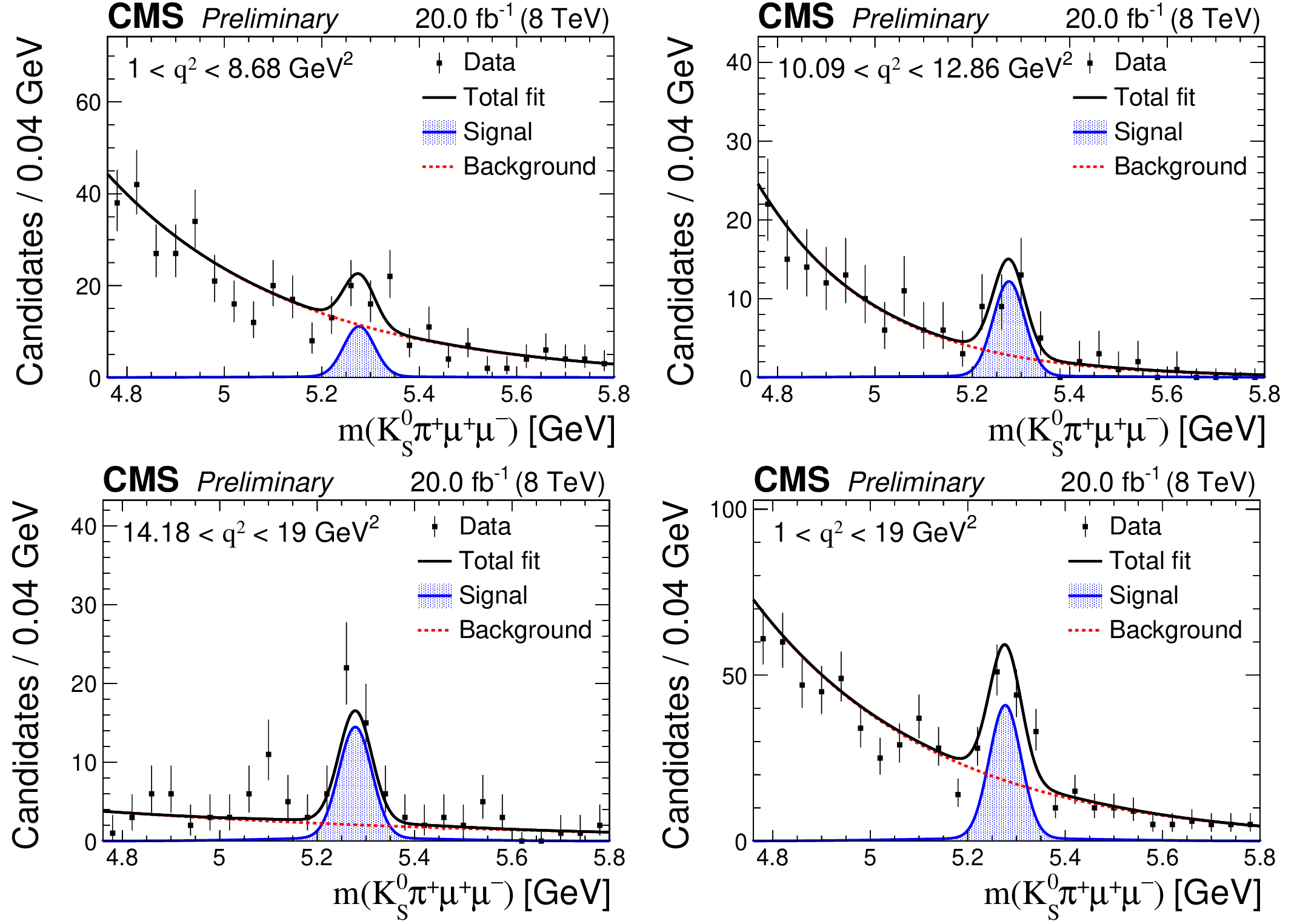
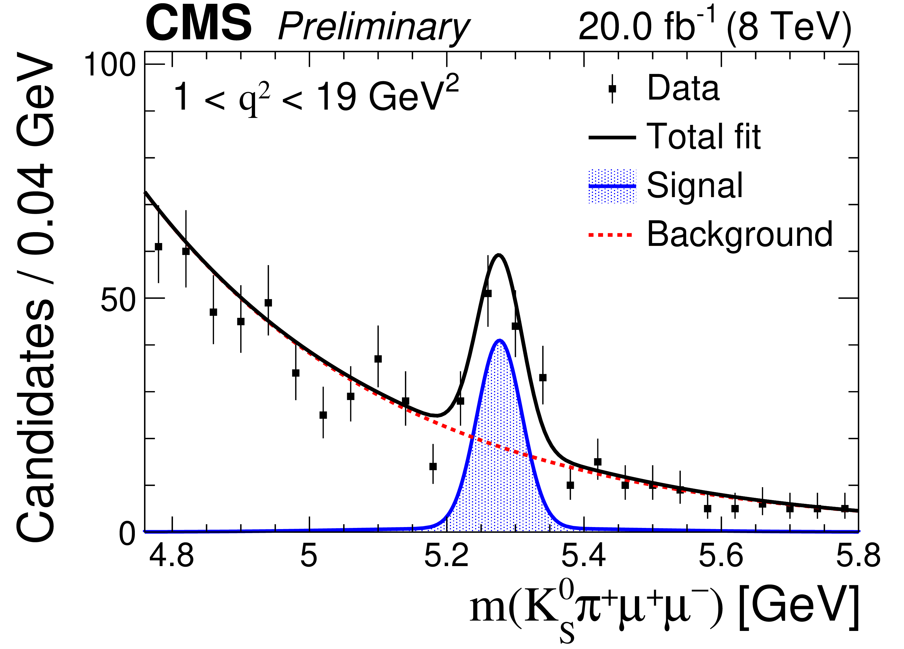
Figure 3:
The fitted $\mathrm{B^{+}}$ invariant mass, $\mathrm {m}$, for each ${q^2}$ range from the three-dimensional fit to the data. The filled area, dashed lines, and solid lines represent the signal, background, and total contributions, respectively. The vertical bars represent the statistical uncertainty. |
png pdf |
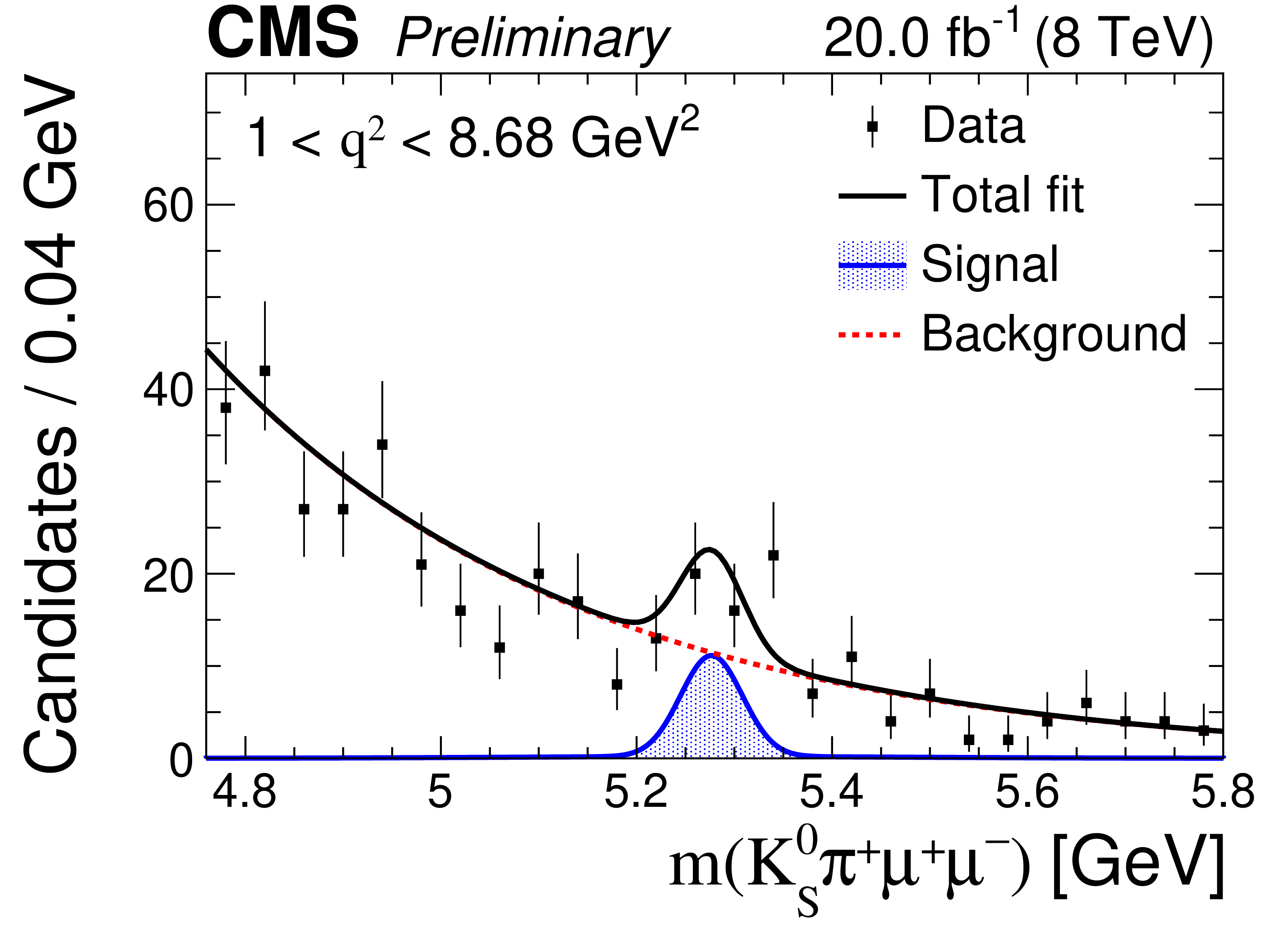
Figure 3-a:
The fitted $\mathrm{B^{+}}$ invariant mass, $\mathrm {m}$, for each ${q^2}$ range from the three-dimensional fit to the data. The filled area, dashed lines, and solid lines represent the signal, background, and total contributions, respectively. The vertical bars represent the statistical uncertainty. |
png pdf |
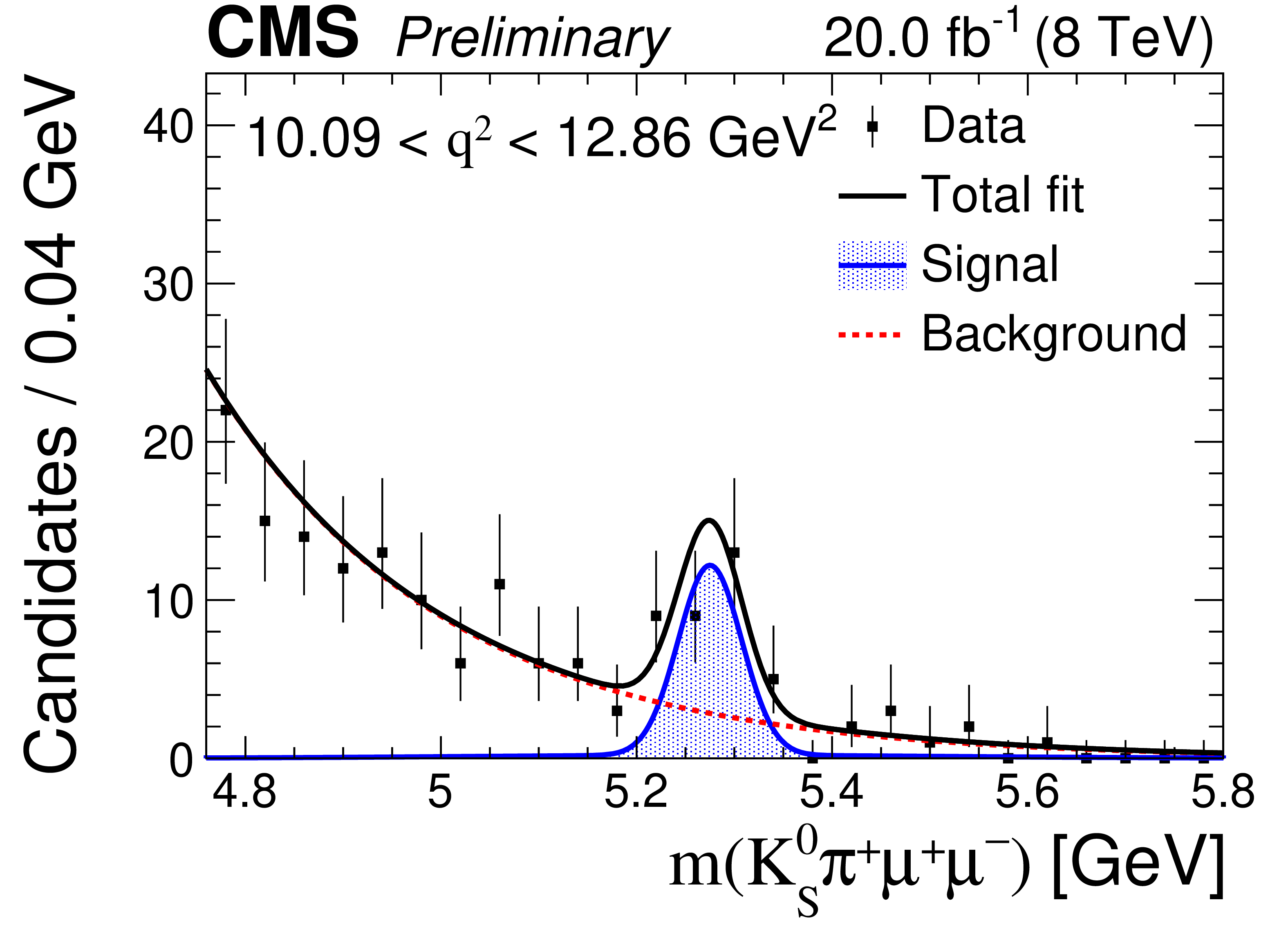
Figure 3-b:
The fitted $\mathrm{B^{+}}$ invariant mass, $\mathrm {m}$, for each ${q^2}$ range from the three-dimensional fit to the data. The filled area, dashed lines, and solid lines represent the signal, background, and total contributions, respectively. The vertical bars represent the statistical uncertainty. |
png pdf |
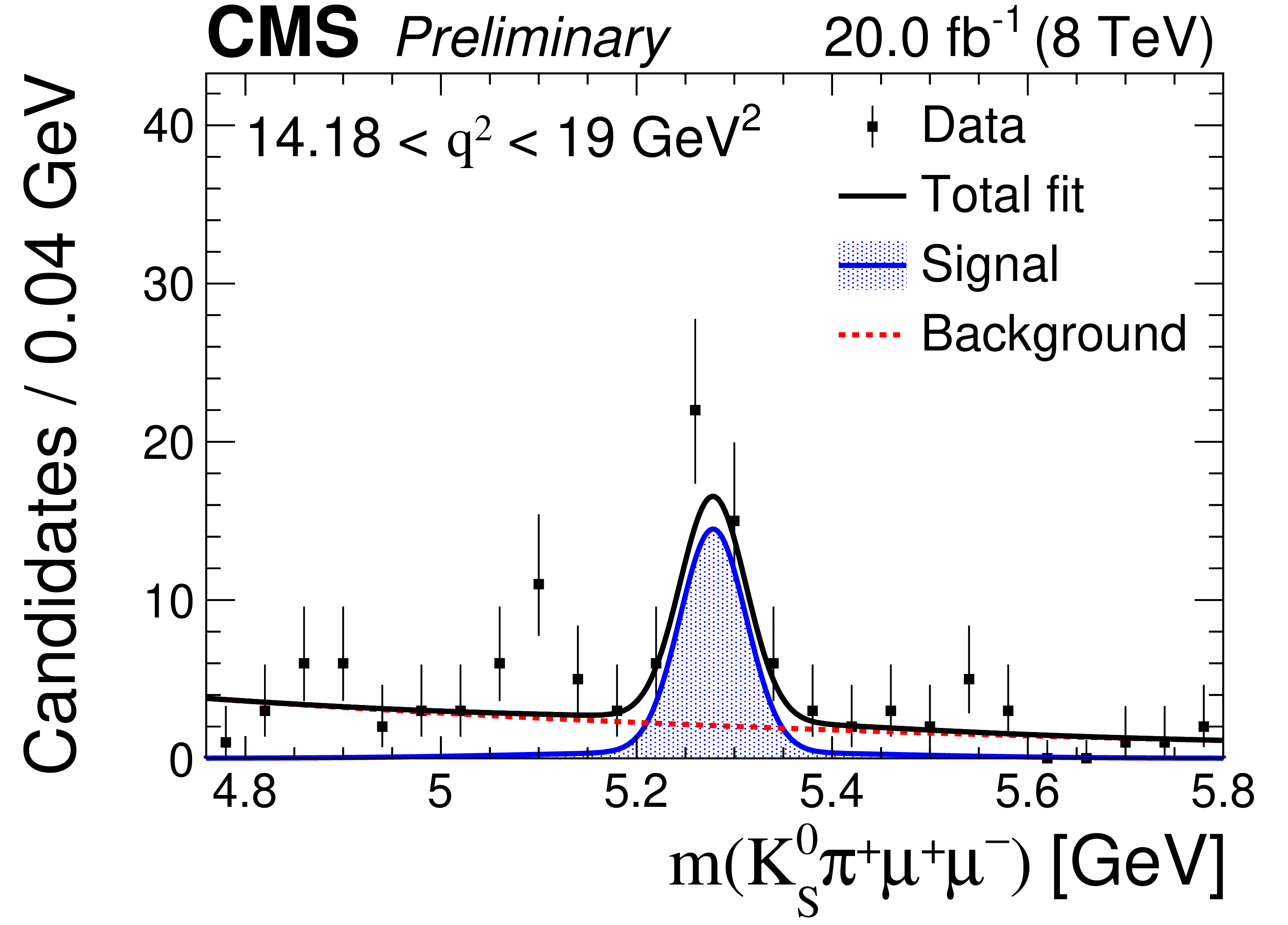
Figure 3-c:
The fitted $\mathrm{B^{+}}$ invariant mass, $\mathrm {m}$, for each ${q^2}$ range from the three-dimensional fit to the data. The filled area, dashed lines, and solid lines represent the signal, background, and total contributions, respectively. The vertical bars represent the statistical uncertainty. |
png pdf |
Figure 3-d:
The fitted $\mathrm{B^{+}}$ invariant mass, $\mathrm {m}$, for each ${q^2}$ range from the three-dimensional fit to the data. The filled area, dashed lines, and solid lines represent the signal, background, and total contributions, respectively. The vertical bars represent the statistical uncertainty. |
png pdf |
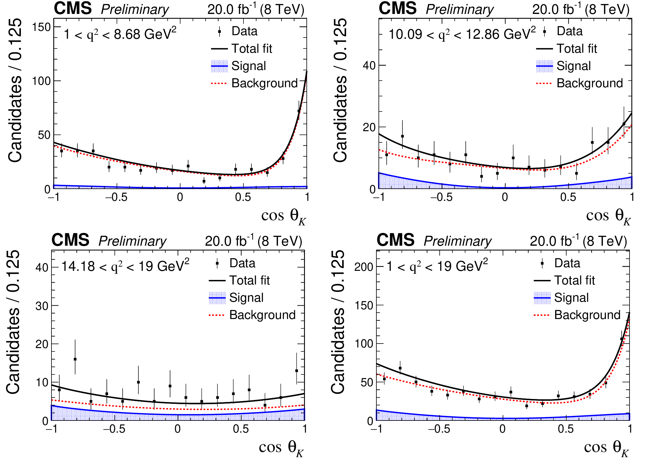
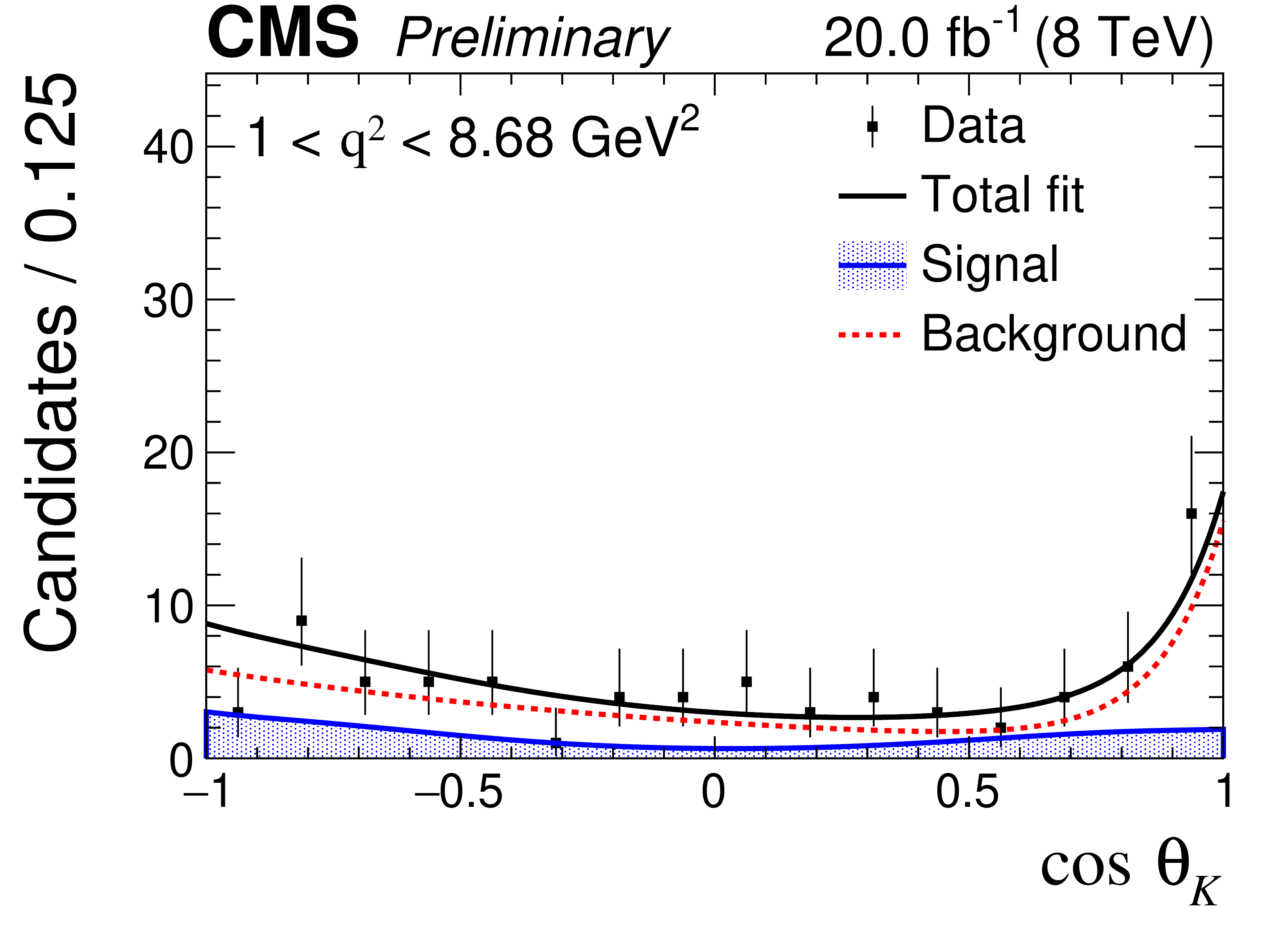
Figure 4:
The fitted angular variable $\cos\theta _{\mathrm{K}}$, for each ${q^2}$ range from the three dimensional fit to the data. The filled area, dashed lines, and solid lines represent the signal, background, and total contributions, respectively. The vertical bars represent the statistical uncertainty. |
png pdf |
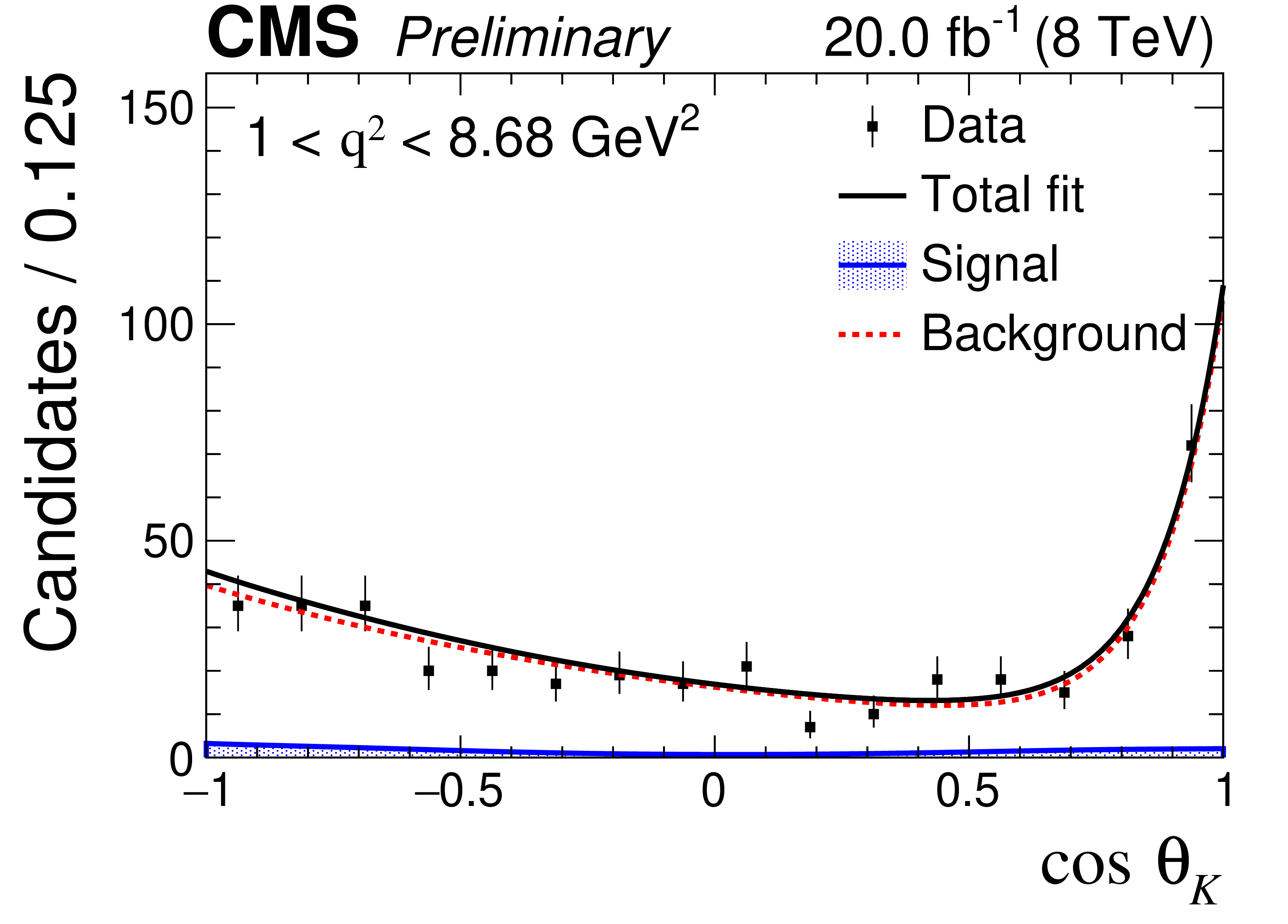
Figure 4-a:
The fitted angular variable $\cos\theta _{\mathrm{K}}$, for each ${q^2}$ range from the three dimensional fit to the data. The filled area, dashed lines, and solid lines represent the signal, background, and total contributions, respectively. The vertical bars represent the statistical uncertainty. |
png pdf |
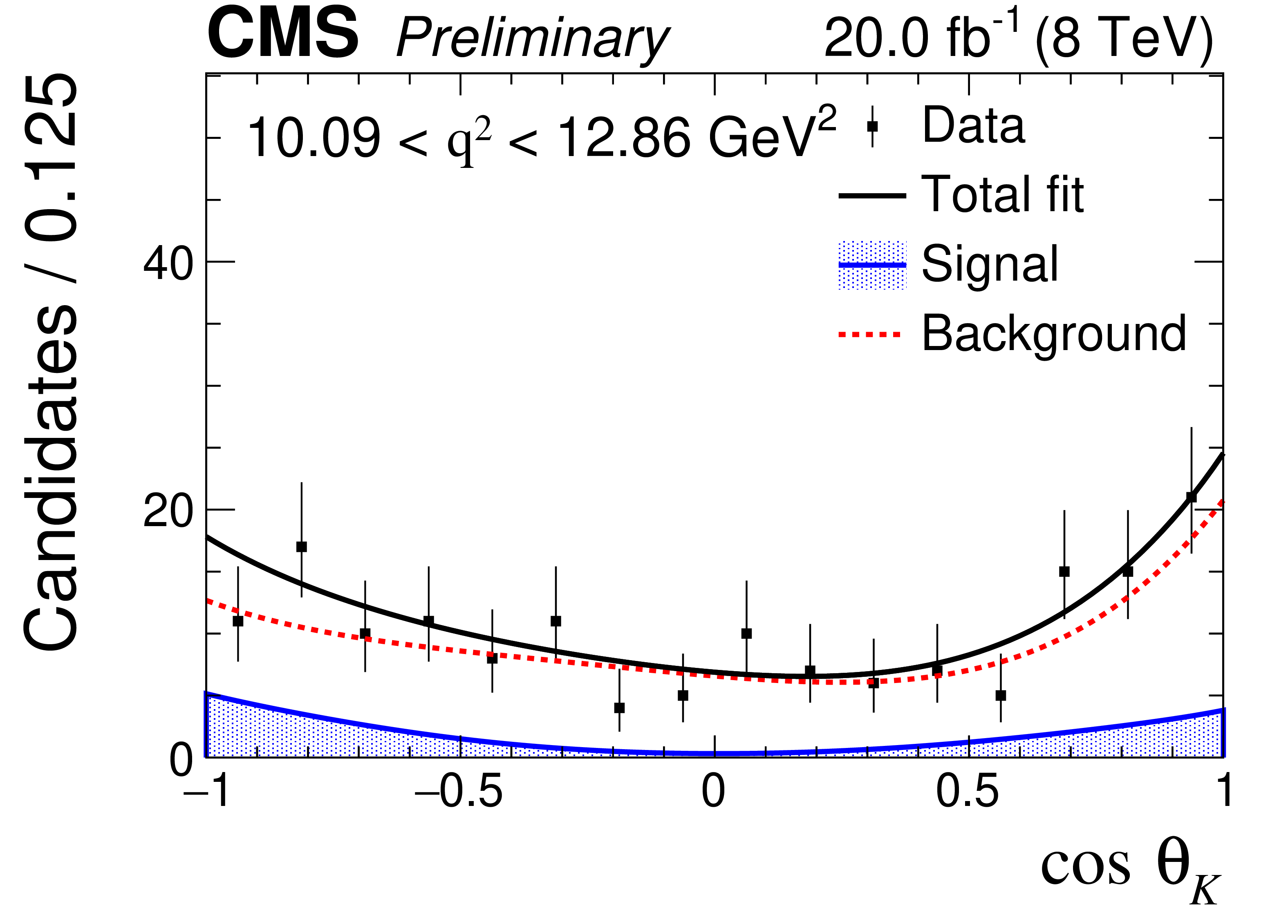
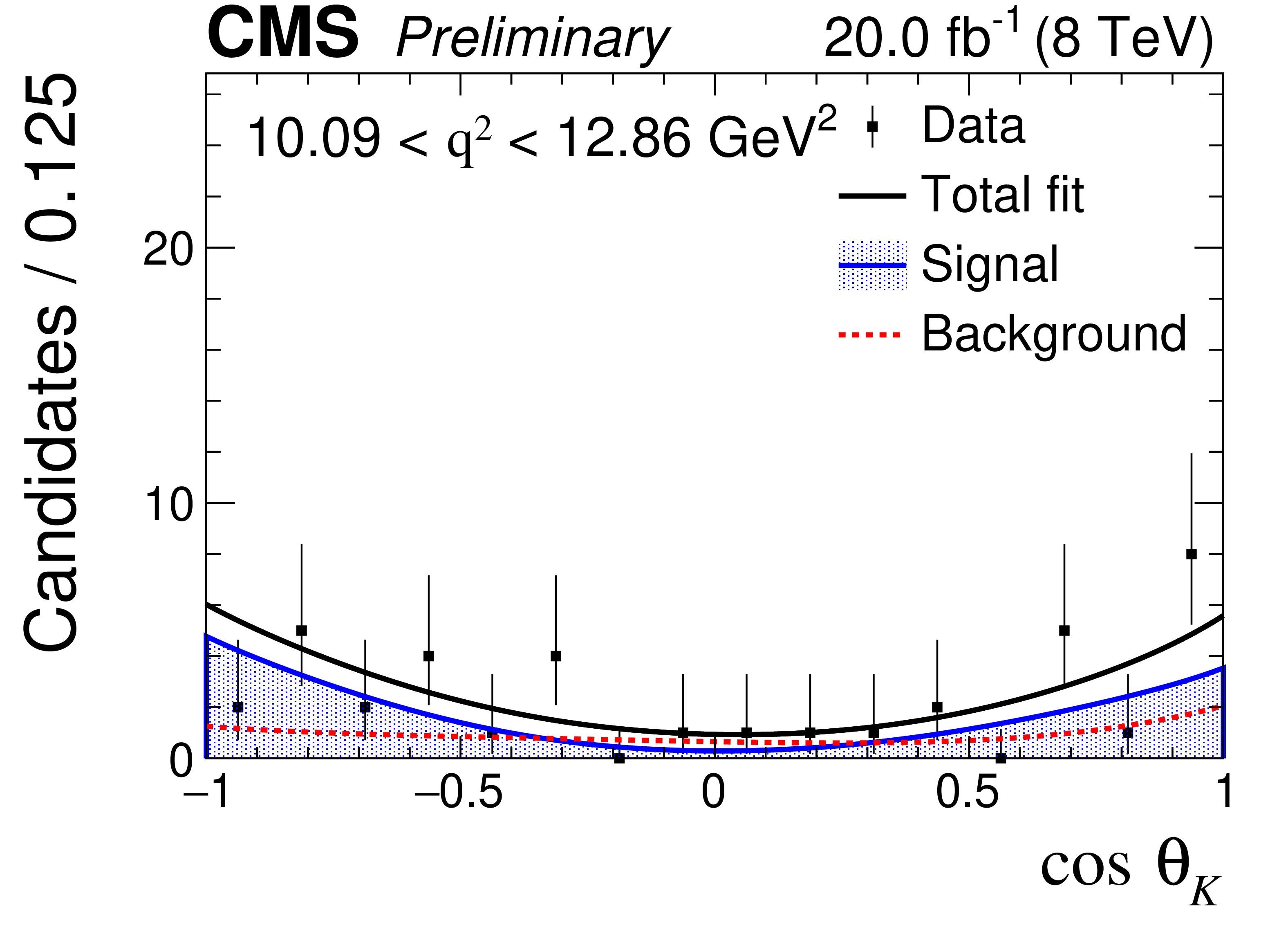
Figure 4-b:
The fitted angular variable $\cos\theta _{\mathrm{K}}$, for each ${q^2}$ range from the three dimensional fit to the data. The filled area, dashed lines, and solid lines represent the signal, background, and total contributions, respectively. The vertical bars represent the statistical uncertainty. |
png pdf |
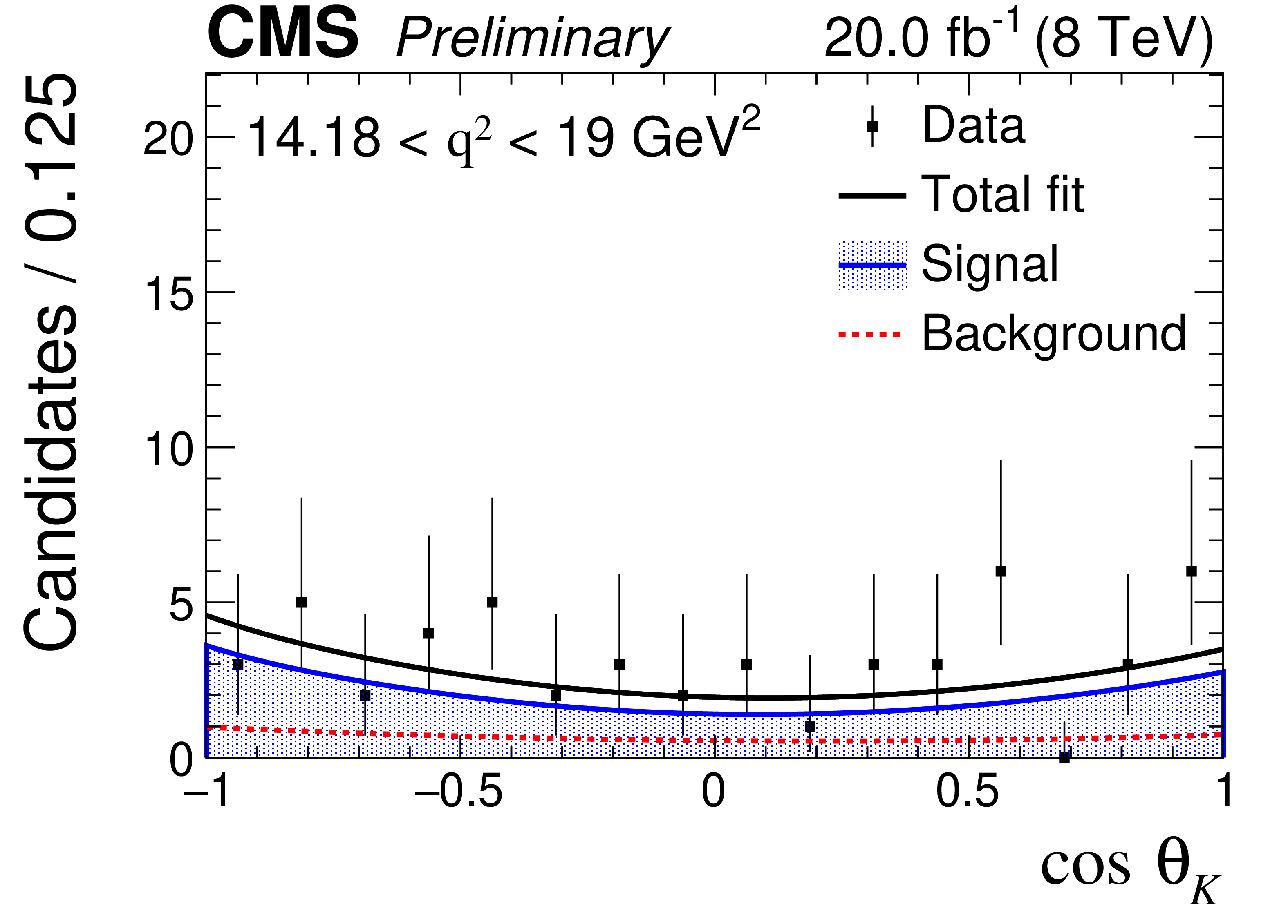
Figure 4-c:
The fitted angular variable $\cos\theta _{\mathrm{K}}$, for each ${q^2}$ range from the three dimensional fit to the data. The filled area, dashed lines, and solid lines represent the signal, background, and total contributions, respectively. The vertical bars represent the statistical uncertainty. |
png pdf |
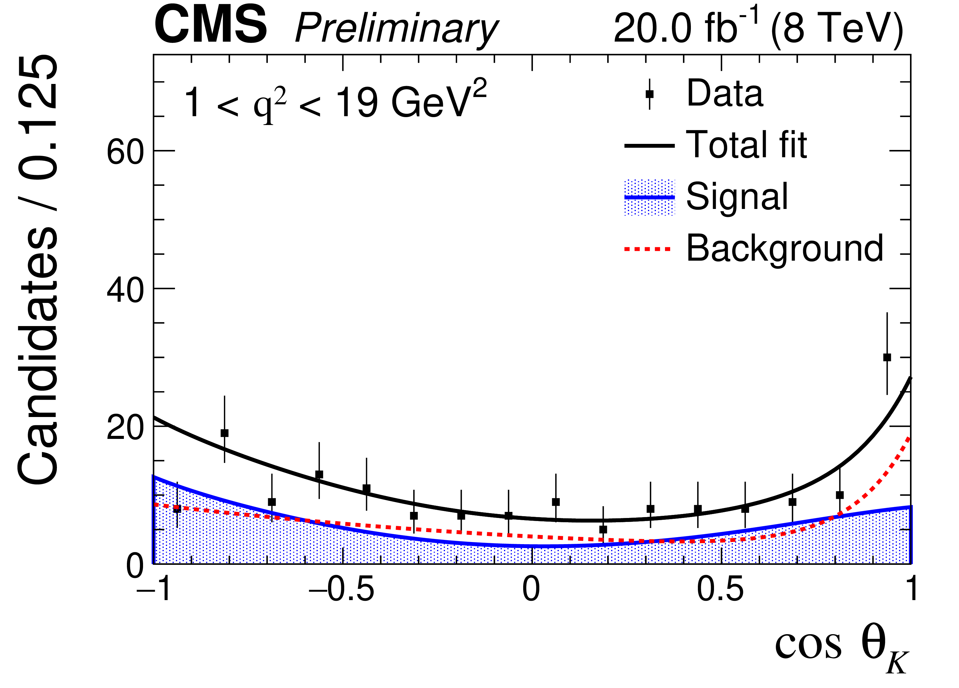
Figure 4-d:
The fitted angular variable $\cos\theta _{\mathrm{K}}$, for each ${q^2}$ range from the three dimensional fit to the data. The filled area, dashed lines, and solid lines represent the signal, background, and total contributions, respectively. The vertical bars represent the statistical uncertainty. |
png pdf |
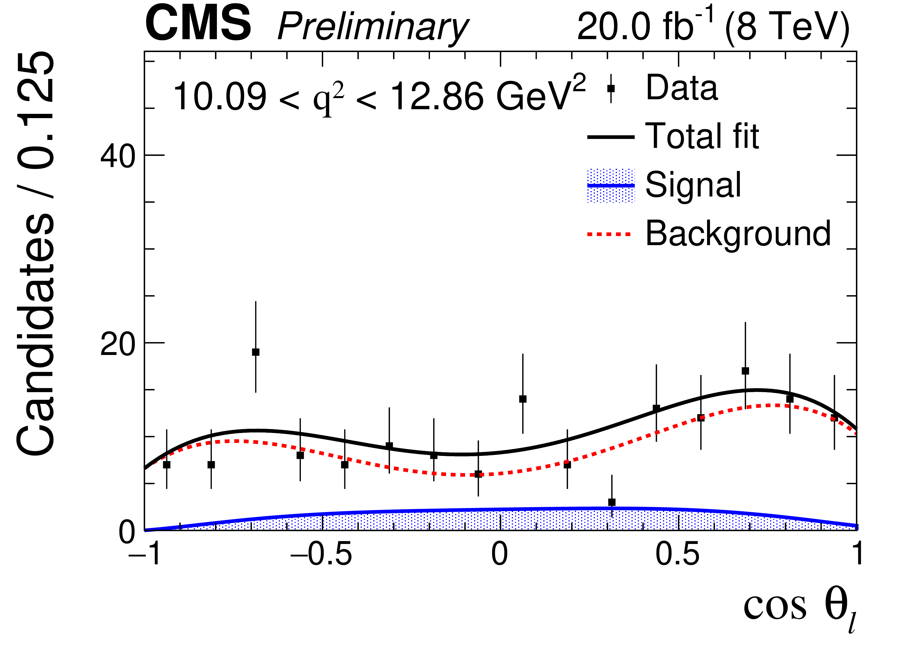
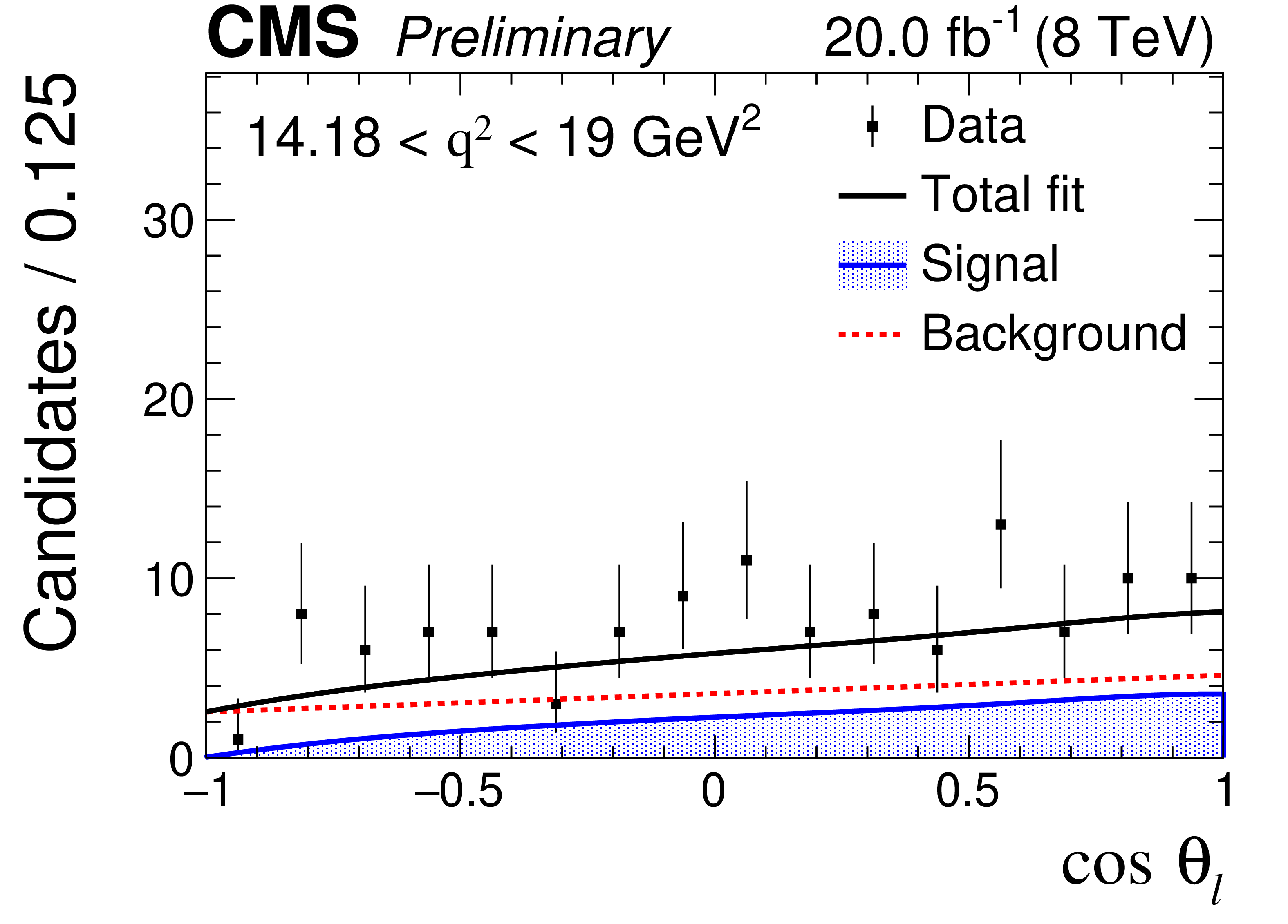
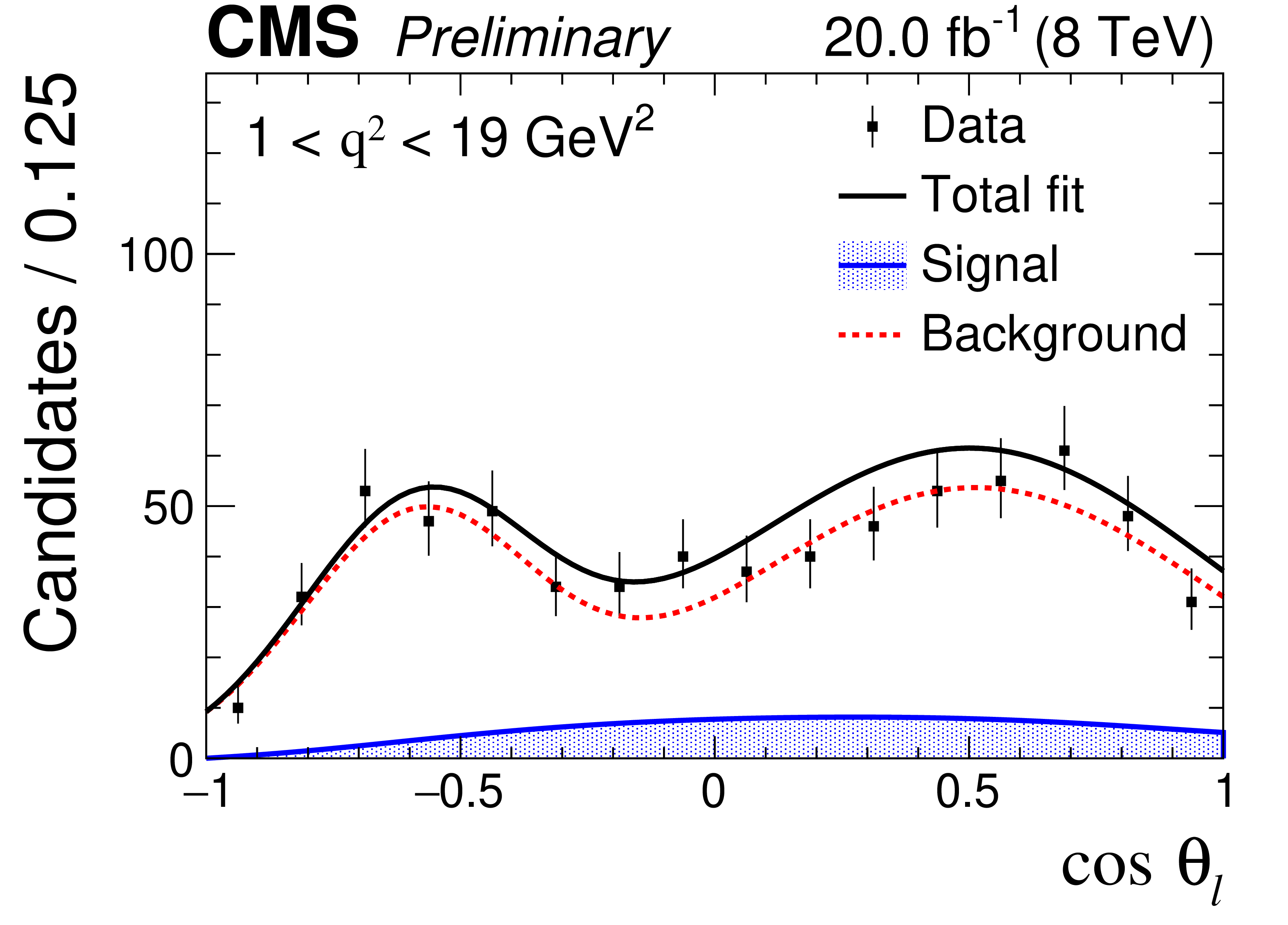
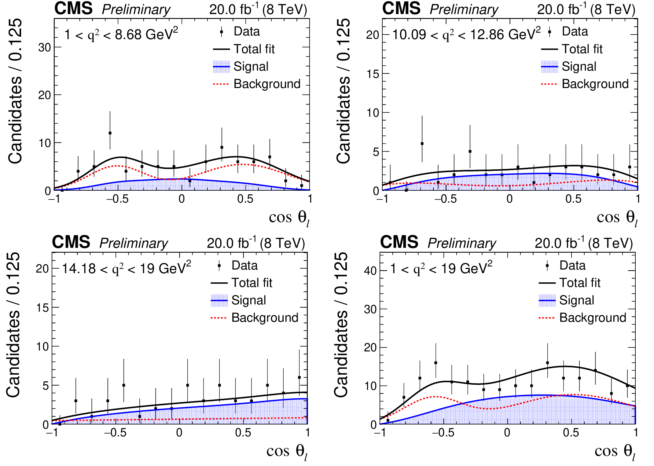
Figure 5:
The fitted angular variable $\cos\theta _{\ell} $, for each ${q^2}$ range from the three-dimensional fit to the data. The filled area, dashed lines, and solid lines represent the signal, background, and total contributions, respectively. The vertical bars on the points represent the statistical uncertainty. |
png pdf |
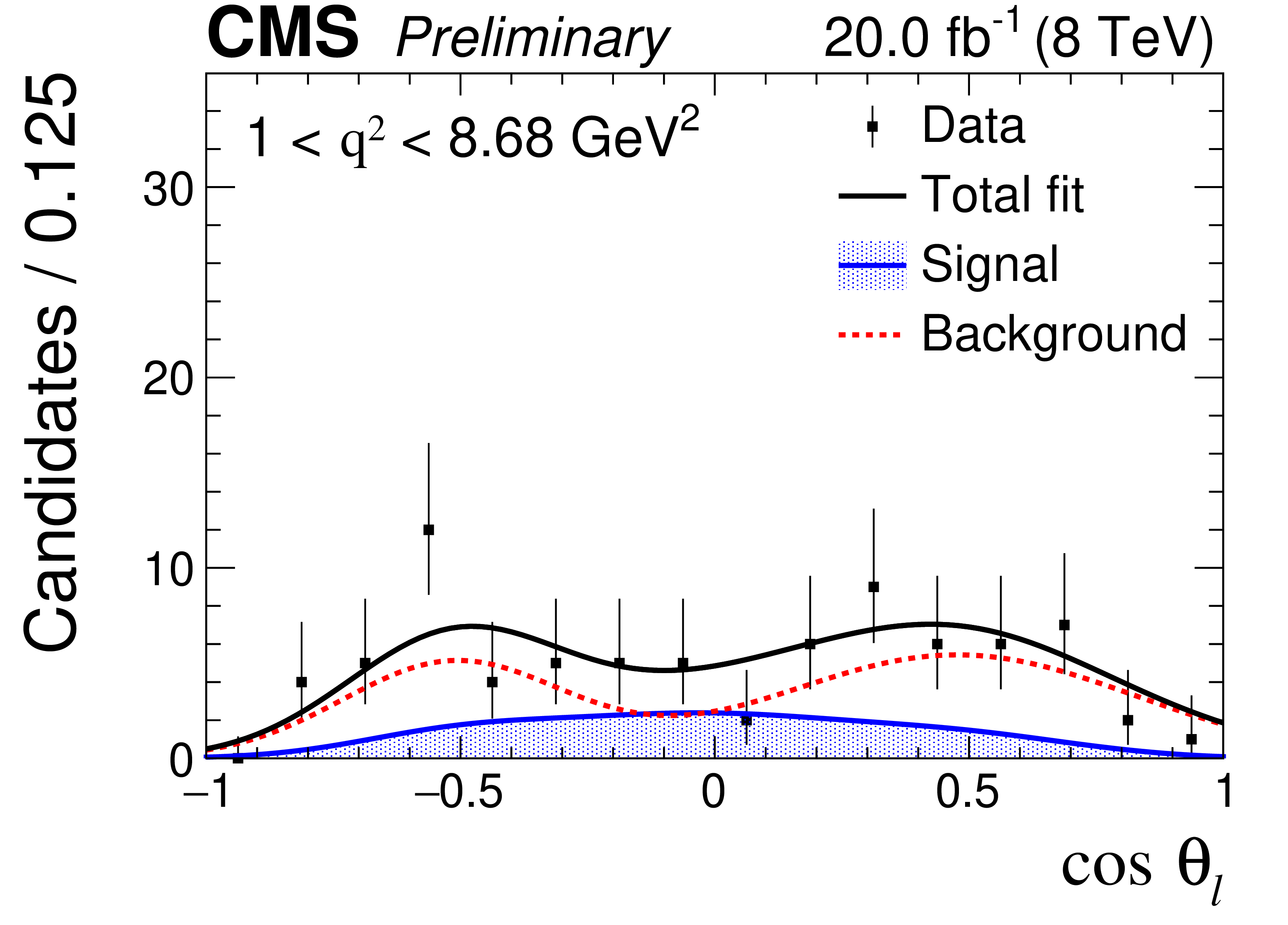
Figure 5-a:
The fitted angular variable $\cos\theta _{\ell} $, for each ${q^2}$ range from the three-dimensional fit to the data. The filled area, dashed lines, and solid lines represent the signal, background, and total contributions, respectively. The vertical bars on the points represent the statistical uncertainty. |
png pdf |
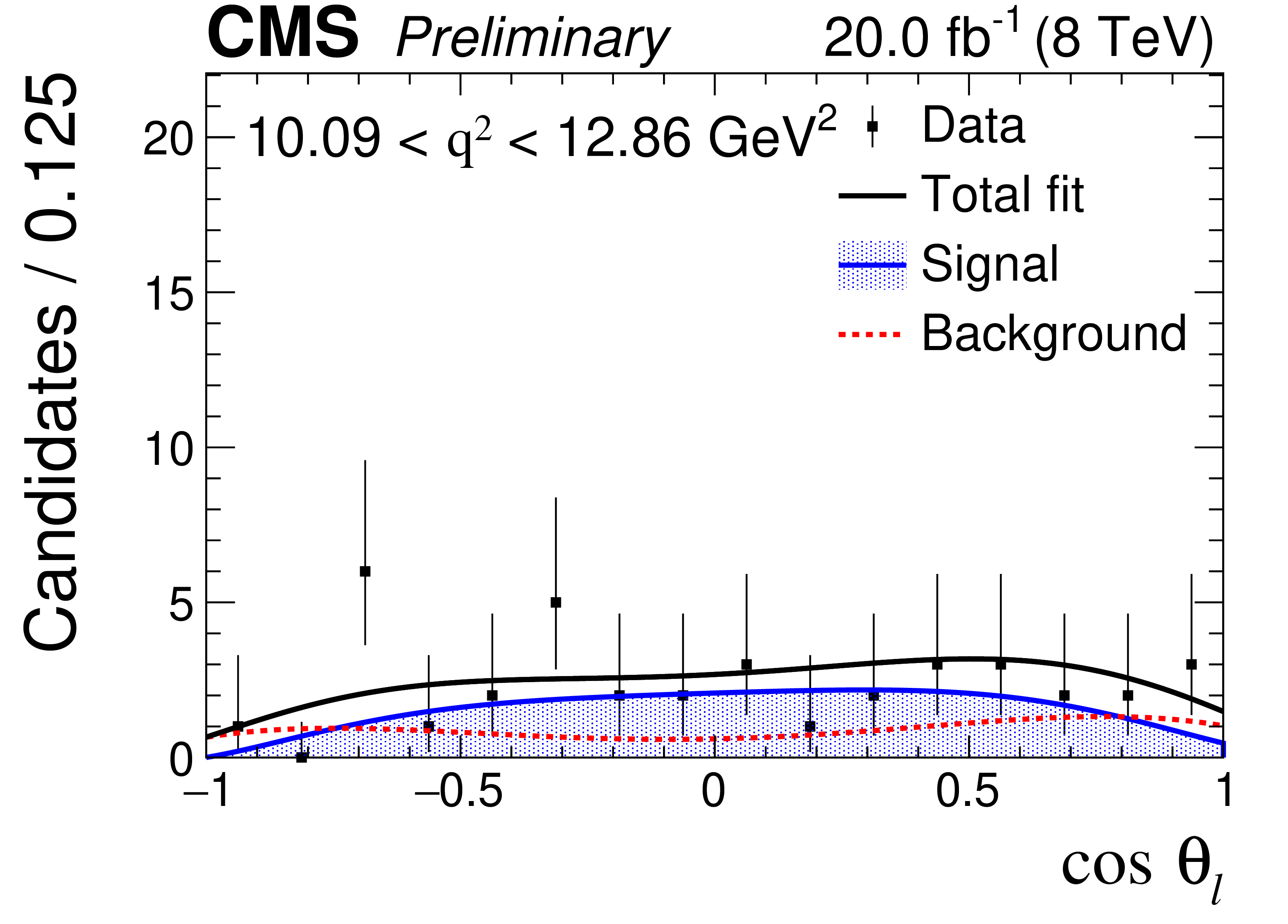
Figure 5-b:
The fitted angular variable $\cos\theta _{\ell} $, for each ${q^2}$ range from the three-dimensional fit to the data. The filled area, dashed lines, and solid lines represent the signal, background, and total contributions, respectively. The vertical bars on the points represent the statistical uncertainty. |
png pdf |
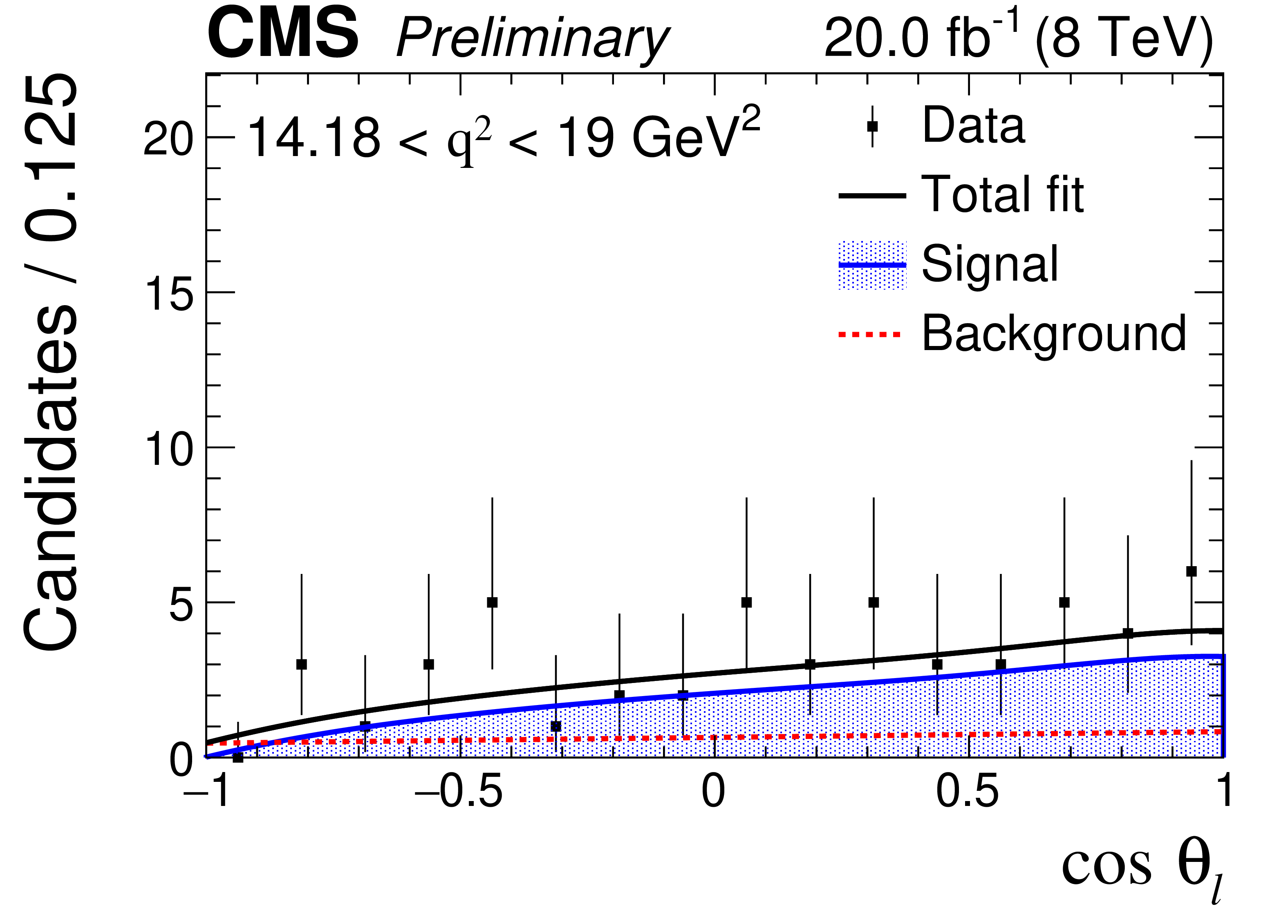
Figure 5-c:
The fitted angular variable $\cos\theta _{\ell} $, for each ${q^2}$ range from the three-dimensional fit to the data. The filled area, dashed lines, and solid lines represent the signal, background, and total contributions, respectively. The vertical bars on the points represent the statistical uncertainty. |
png pdf |
Figure 5-d:
The fitted angular variable $\cos\theta _{\ell} $, for each ${q^2}$ range from the three-dimensional fit to the data. The filled area, dashed lines, and solid lines represent the signal, background, and total contributions, respectively. The vertical bars on the points represent the statistical uncertainty. |
png pdf |
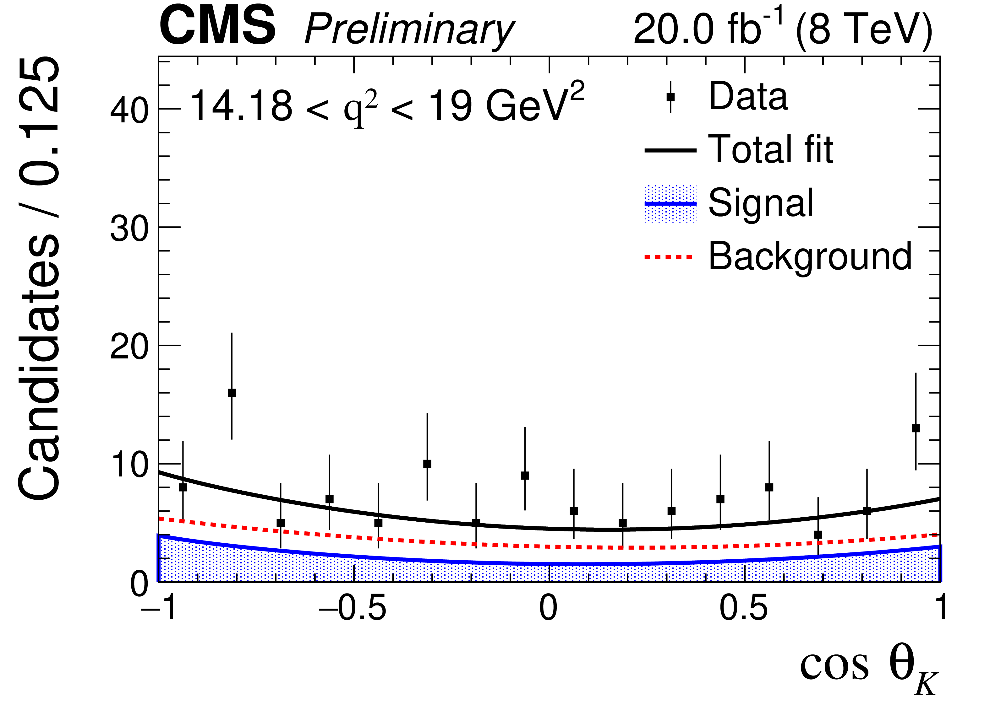
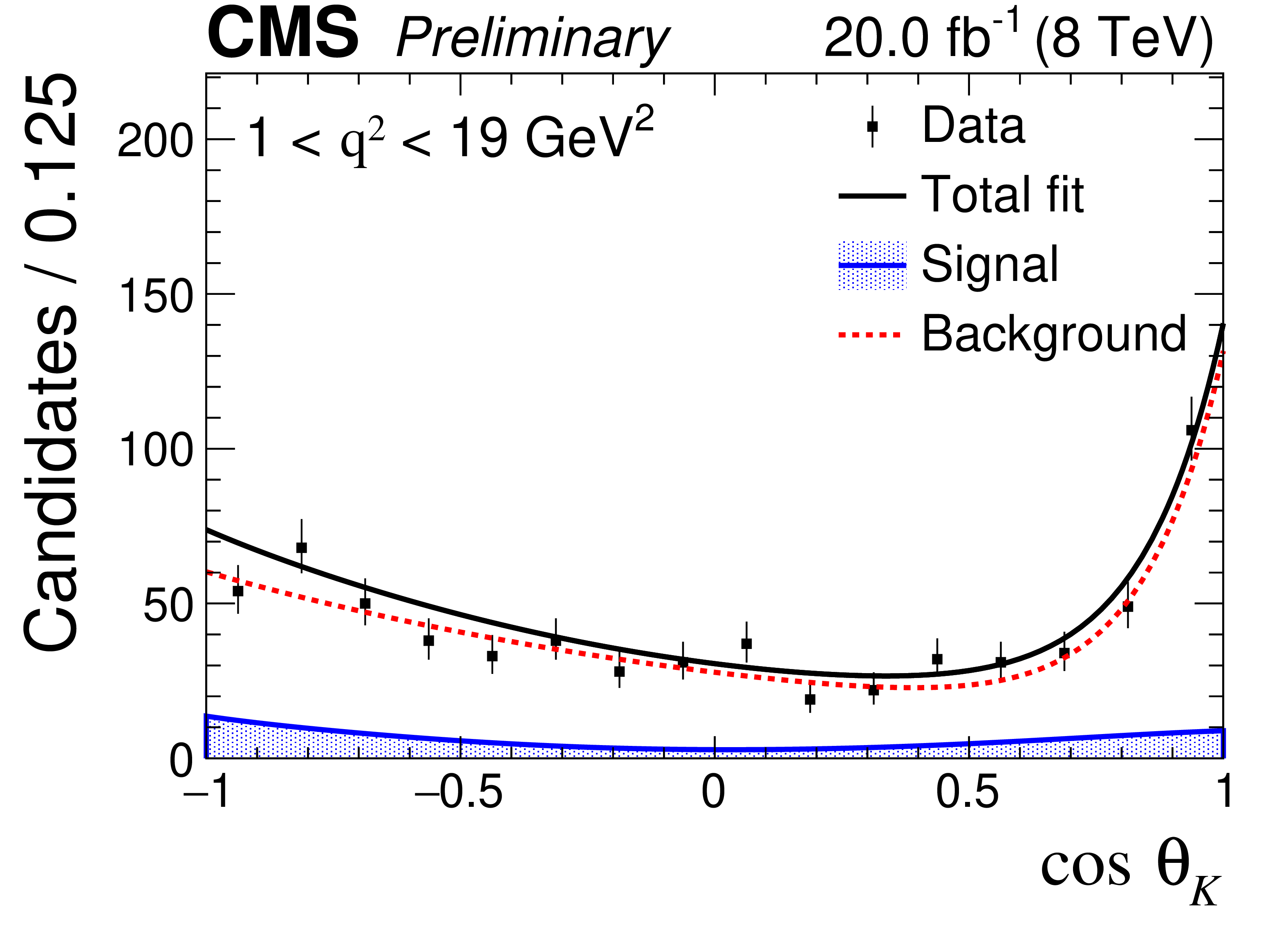
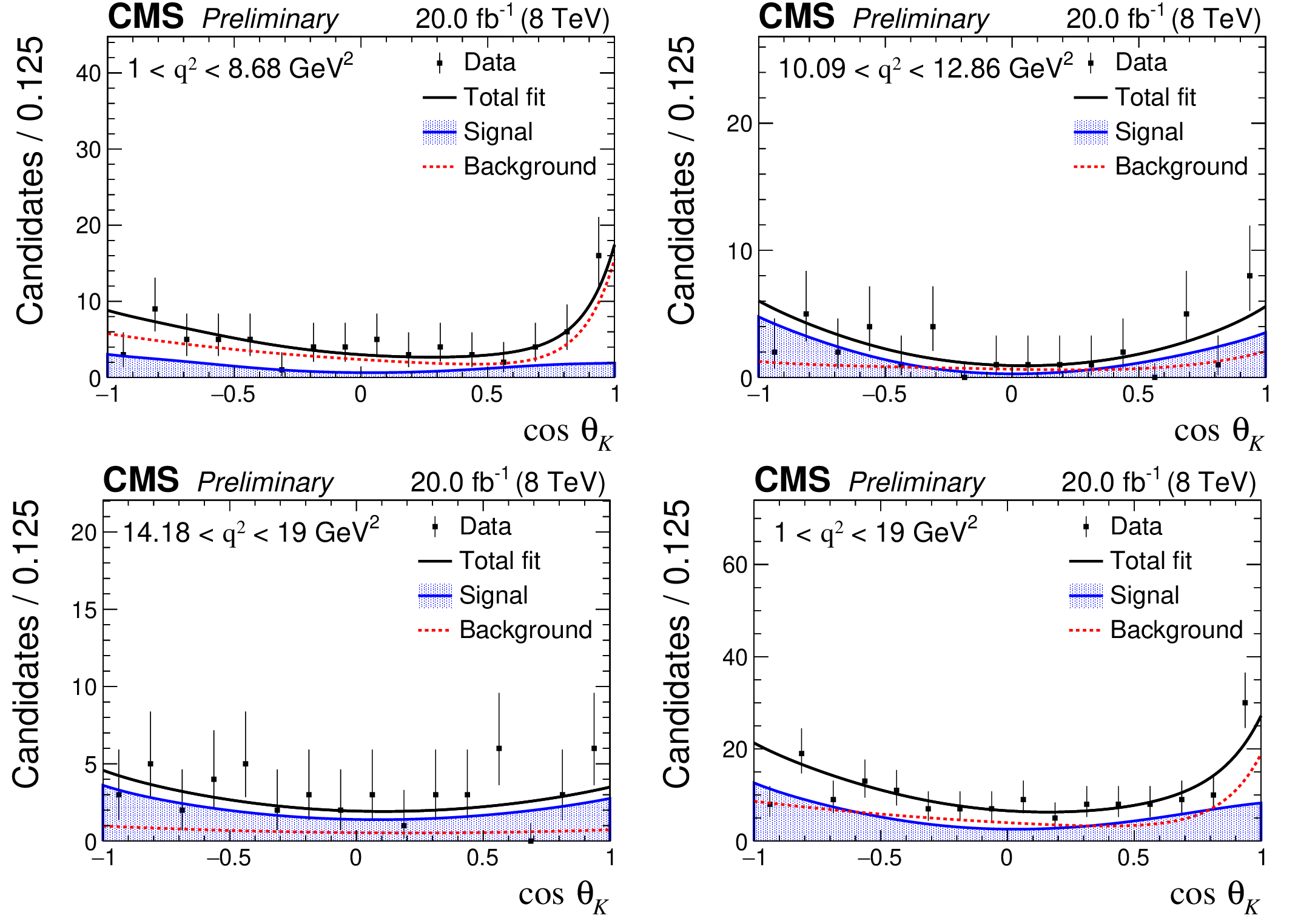
Figure 6:
The angular variable $\cos\theta _{\mathrm{K}}$ for the events in the signal region 5.18 $ < m < $ 5.38 GeV, overlayed with the corresponding signal, background and total pdfs obtained from the final fit, for each ${q^2}$ range. The filled area, dashed lines, and solid lines represent the signal, background, and total contributions, respectively. |
png pdf |
Figure 6-a:
The angular variable $\cos\theta _{\mathrm{K}}$ for the events in the signal region 5.18 $ < m < $ 5.38 GeV, overlayed with the corresponding signal, background and total pdfs obtained from the final fit, for each ${q^2}$ range. The filled area, dashed lines, and solid lines represent the signal, background, and total contributions, respectively. |
png pdf |
Figure 6-b:
The angular variable $\cos\theta _{\mathrm{K}}$ for the events in the signal region 5.18 $ < m < $ 5.38 GeV, overlayed with the corresponding signal, background and total pdfs obtained from the final fit, for each ${q^2}$ range. The filled area, dashed lines, and solid lines represent the signal, background, and total contributions, respectively. |
png pdf |
Figure 6-c:
The angular variable $\cos\theta _{\mathrm{K}}$ for the events in the signal region 5.18 $ < m < $ 5.38 GeV, overlayed with the corresponding signal, background and total pdfs obtained from the final fit, for each ${q^2}$ range. The filled area, dashed lines, and solid lines represent the signal, background, and total contributions, respectively. |
png pdf |
Figure 6-d:
The angular variable $\cos\theta _{\mathrm{K}}$ for the events in the signal region 5.18 $ < m < $ 5.38 GeV, overlayed with the corresponding signal, background and total pdfs obtained from the final fit, for each ${q^2}$ range. The filled area, dashed lines, and solid lines represent the signal, background, and total contributions, respectively. |
png pdf |
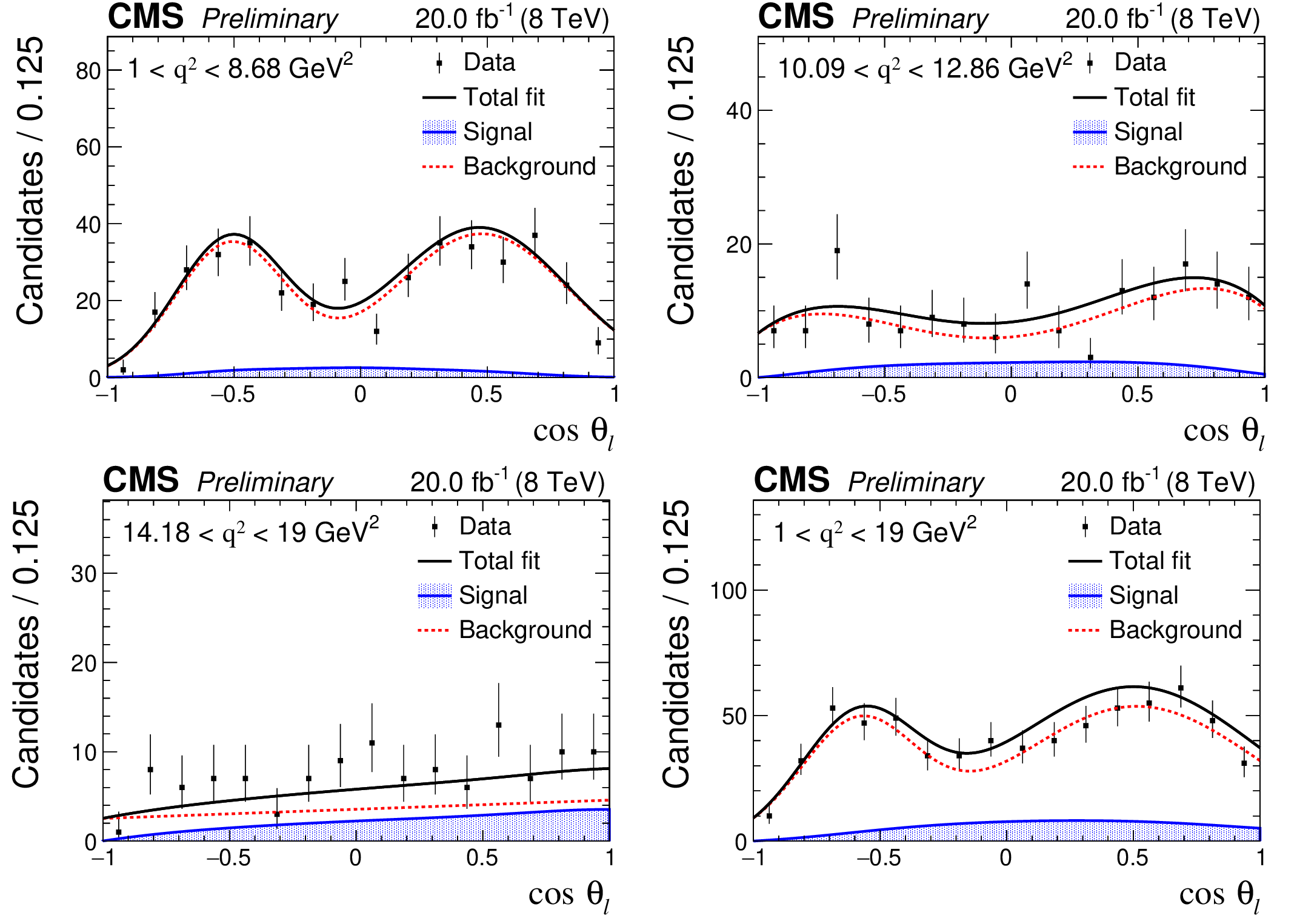
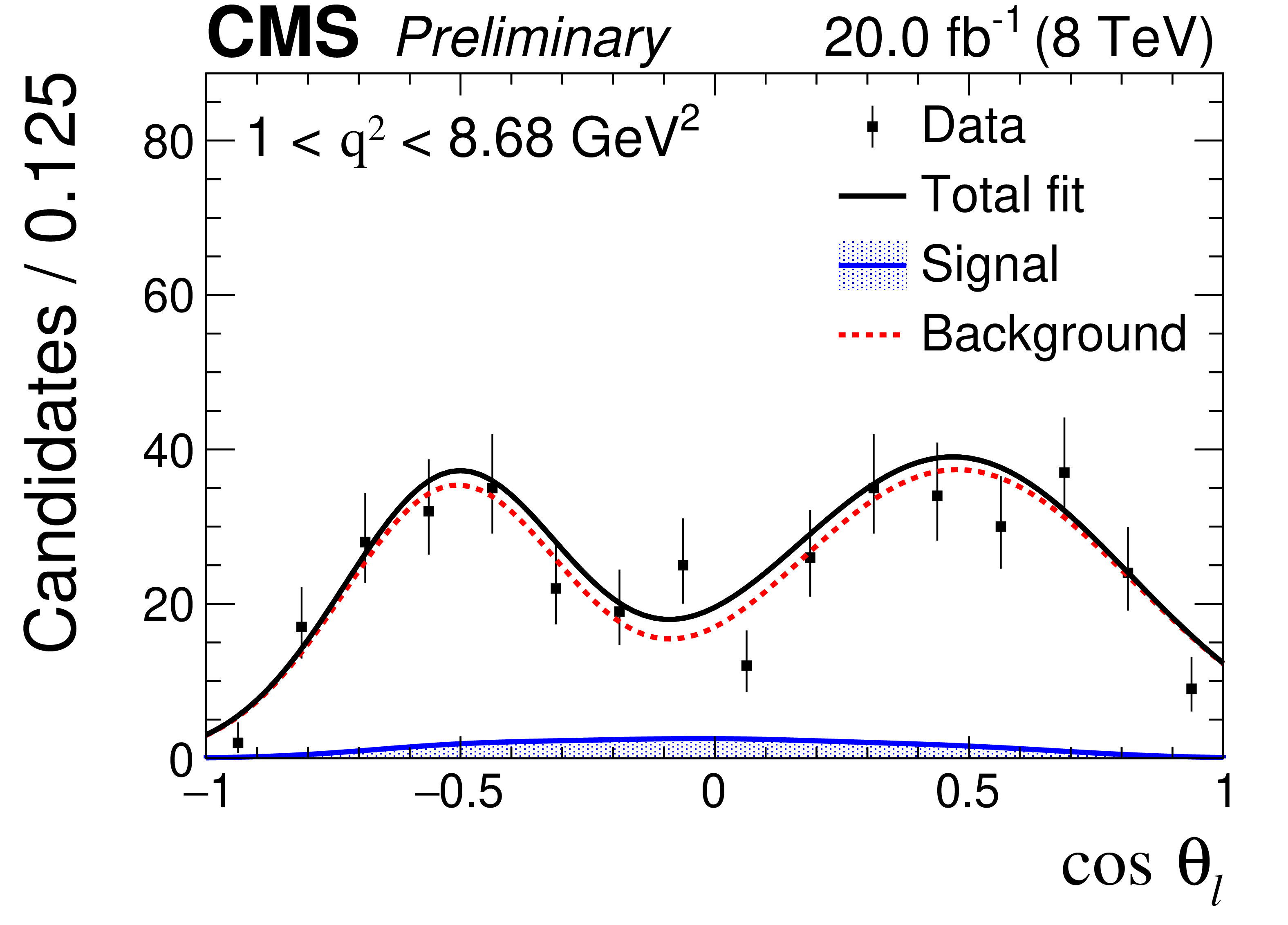
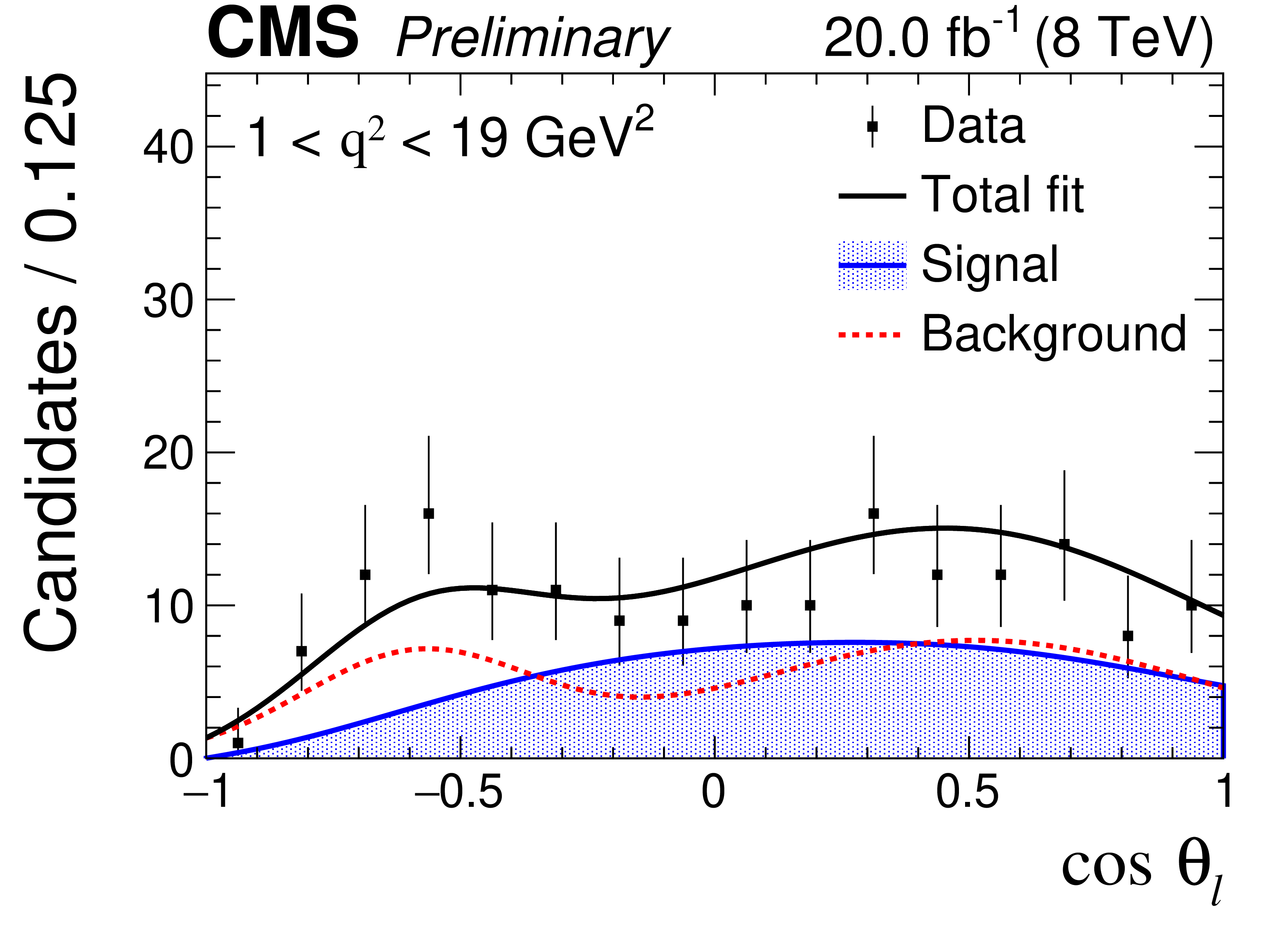
Figure 7:
The angular variable $\cos\theta _{\ell} $ for the events in the signal region 5.18 $ < m < $ 5.38 GeV, overlayed with the corresponding signal, background and total pdfs obtained from the final fit, for each ${q^2}$ range. The filled area, dashed lines, and solid lines represent the signal, background, and total contributions, respectively. |
png pdf |
Figure 7-a:
The angular variable $\cos\theta _{\ell} $ for the events in the signal region 5.18 $ < m < $ 5.38 GeV, overlayed with the corresponding signal, background and total pdfs obtained from the final fit, for each ${q^2}$ range. The filled area, dashed lines, and solid lines represent the signal, background, and total contributions, respectively. |
png pdf |
Figure 7-b:
The angular variable $\cos\theta _{\ell} $ for the events in the signal region 5.18 $ < m < $ 5.38 GeV, overlayed with the corresponding signal, background and total pdfs obtained from the final fit, for each ${q^2}$ range. The filled area, dashed lines, and solid lines represent the signal, background, and total contributions, respectively. |
png pdf |
Figure 7-c:
The angular variable $\cos\theta _{\ell} $ for the events in the signal region 5.18 $ < m < $ 5.38 GeV, overlayed with the corresponding signal, background and total pdfs obtained from the final fit, for each ${q^2}$ range. The filled area, dashed lines, and solid lines represent the signal, background, and total contributions, respectively. |
png pdf |
Figure 7-d:
The angular variable $\cos\theta _{\ell} $ for the events in the signal region 5.18 $ < m < $ 5.38 GeV, overlayed with the corresponding signal, background and total pdfs obtained from the final fit, for each ${q^2}$ range. The filled area, dashed lines, and solid lines represent the signal, background, and total contributions, respectively. |
png pdf |
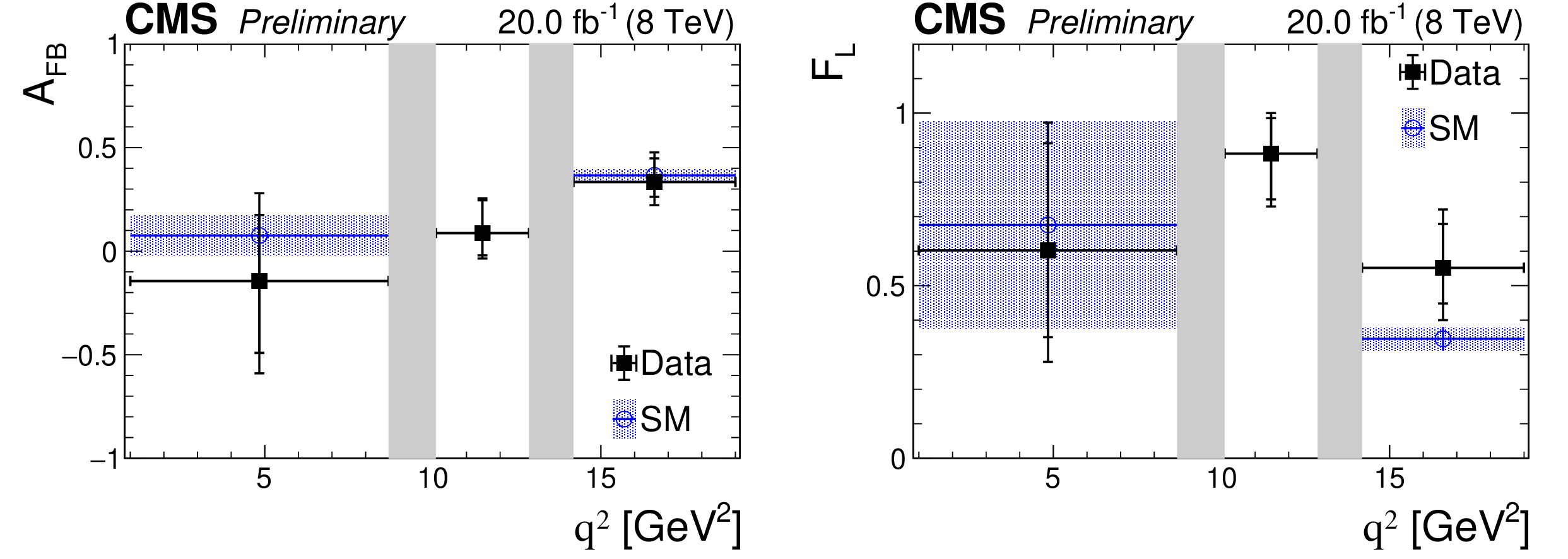
Figure 8:
The measured values of ${A_\mathrm {FB}}$ and ${F_\mathrm {L}}$ versus ${q^2}$ for ${\mathrm{B^{+}} \to {{\mathrm{K}} ^{*+}} \mu^{+} \mu^{-}}$ decays. The statistical (total) uncertainty is shown by inner (outer) vertical bars. The vertical shaded regions correspond to the ${\mathrm{B^{+}} \to {{\mathrm{K}} ^{*+}} {\mathrm{J}/\psi} (\mu^{+} \mu^{-})}$ and ${\mathrm{B^{+}} \to {{\mathrm{K}} ^{*+}} \psi(\text{2S})(\mu^{+} \mu^{-})}$ dominated regions. The blue band shows the SM predictions for the corresponding ${q^2}$ range. |
png pdf |
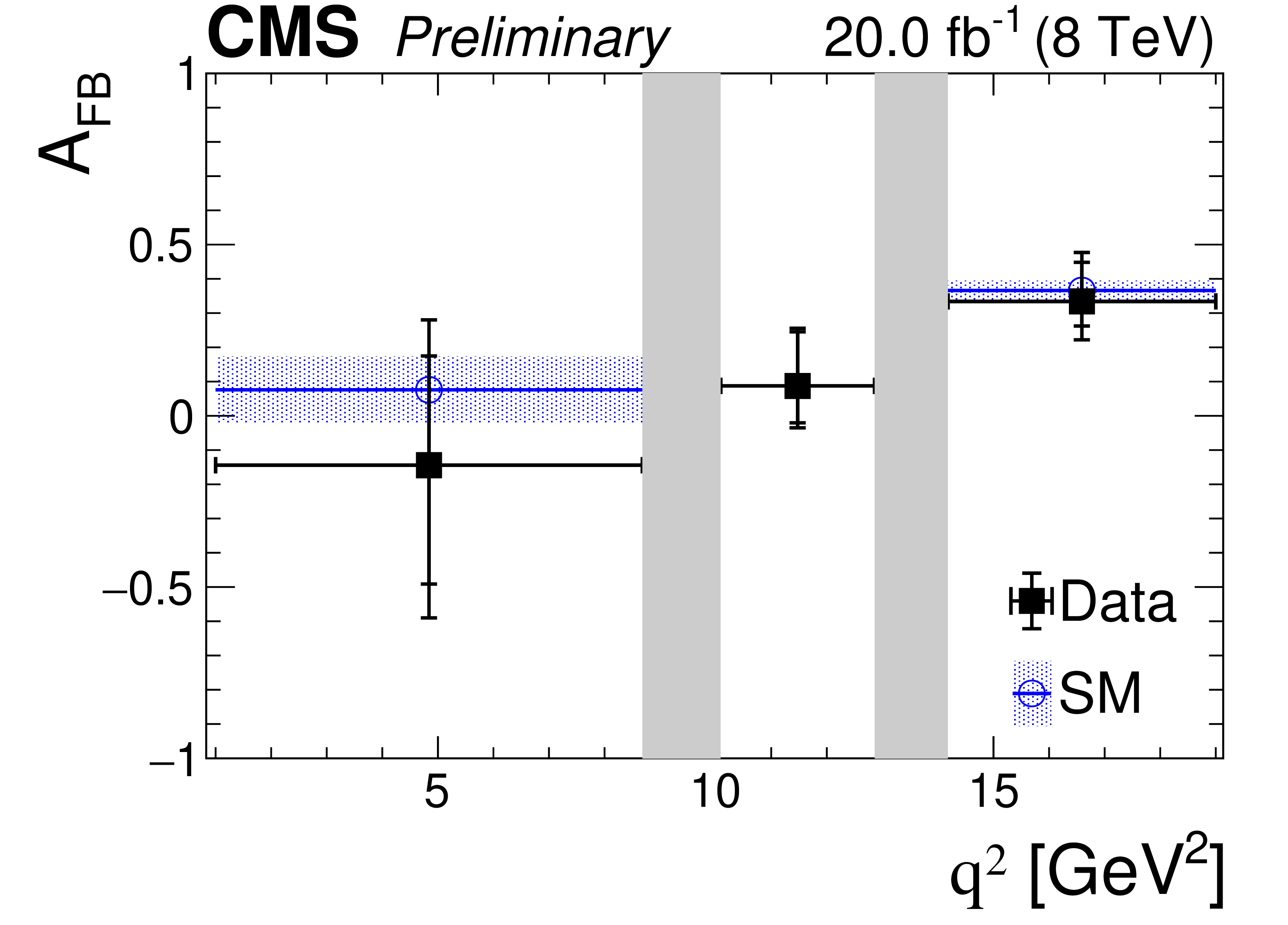
Figure 8-a:
The measured values of ${A_\mathrm {FB}}$ and ${F_\mathrm {L}}$ versus ${q^2}$ for ${\mathrm{B^{+}} \to {{\mathrm{K}} ^{*+}} \mu^{+} \mu^{-}}$ decays. The statistical (total) uncertainty is shown by inner (outer) vertical bars. The vertical shaded regions correspond to the ${\mathrm{B^{+}} \to {{\mathrm{K}} ^{*+}} {\mathrm{J}/\psi} (\mu^{+} \mu^{-})}$ and ${\mathrm{B^{+}} \to {{\mathrm{K}} ^{*+}} \psi(\text{2S})(\mu^{+} \mu^{-})}$ dominated regions. The blue band shows the SM predictions for the corresponding ${q^2}$ range. |
png pdf |
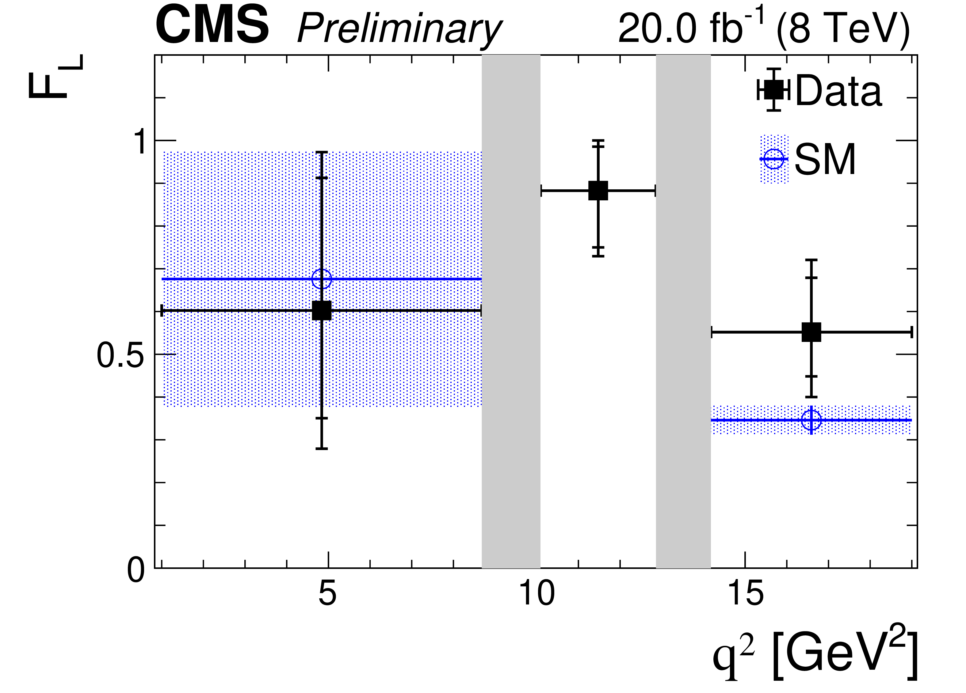
Figure 8-b:
The measured values of ${A_\mathrm {FB}}$ and ${F_\mathrm {L}}$ versus ${q^2}$ for ${\mathrm{B^{+}} \to {{\mathrm{K}} ^{*+}} \mu^{+} \mu^{-}}$ decays. The statistical (total) uncertainty is shown by inner (outer) vertical bars. The vertical shaded regions correspond to the ${\mathrm{B^{+}} \to {{\mathrm{K}} ^{*+}} {\mathrm{J}/\psi} (\mu^{+} \mu^{-})}$ and ${\mathrm{B^{+}} \to {{\mathrm{K}} ^{*+}} \psi(\text{2S})(\mu^{+} \mu^{-})}$ dominated regions. The blue band shows the SM predictions for the corresponding ${q^2}$ range. |
| Tables | |
png pdf |
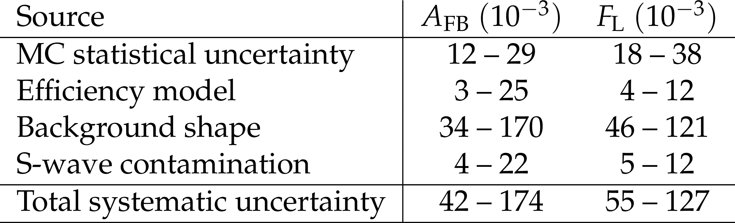
Table 1:
Sources of systematic uncertainties and the effect on ${A_\mathrm {FB}}$ and ${F_\mathrm {L}}$. The values given are absolute and the ranges indicate the variation over the four ${q^2}$ bins. |
png pdf |
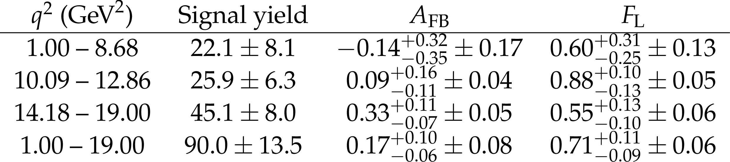
Table 2:
The signal yield with statistical uncertainty and the fitted ${A_\mathrm {FB}}$ and ${F_\mathrm {L}}$ values with statistical and systematic uncertainties, for each ${q^2}$ range. |
| Summary |
| The first angular analysis of the decay ${\mathrm{B^{+}}\to {\mathrm K^{*+}} \mu^{+} \mu^{-}}$ has been performed using a sample of proton-proton collisions at a center-of-mass energy of 8 TeV. The data were collected with the CMS detector in 2012 and correspond to an integrated luminosity of 20.0 fb$^{-1}$ . For each bin of dimuon invariant mass squared (${q^2} $), a three-dimensional unbinned maximum-likelihood fit was performed to the distributions of the ${\mathrm K^{*+}} \mu^{+}\mu^{-}$ invariant mass and two decay angles. The forward-backward asymmetry, ${A_\mathrm{FB}} $, of the muon system and the longitudinal polarization of ${\mathrm K^{*+}} , {F_\mathrm{L}} $, are extracted from the fit and compared with predictions from a standard model prediction. The results are consistent with standard model expectations. |
| References | ||||
| 1 | C. Bobeth, G. Hiller, and D. van Dyk | The benefits of $ \overline{B} \to \overline{K}^* \ell^+ \ell^- $ decays at low recoil | JHEP 07 (2010) 098 | 1006.5013 |
| 2 | C. Bobeth, G. Hiller, D. van Dyk, and C. Wacker | The decay $ \overline{B} \to \overline{K} \ell^+ \ell^- $ at low hadronic recoil and model-independent $ \delta b = $ 1 constraints | JHEP 01 (2012) 107 | 1111.2558 |
| 3 | C. Bobeth, G. Hiller, and D. van Dyk | General analysis of $ \overline{B} \to \overline{K}{}^{(*)} \ell^+ \ell^- $ decays at low recoil | PRD 87 (2012) 034016 | 1212.2321 |
| 4 | A. Ali, G. Kramer, and G. Zhu | $ B\to K^*\ell^+\ell^- $ decay in soft-collinear effective theory | EPJC 47 (2006) 625 | hep-ph/0601034 |
| 5 | W. Altmannshofer et al. | Symmetries and asymmetries of $ B \to K^{*} \mu^{+} \mu^{-} $ decays in the Standard Model and beyond | JHEP 01 (2009) 019 | 0811.1214 |
| 6 | W. Altmannshofer, P. Paradisi, and D. M. Straub | Model-independent constraints on new physics in $ b \to s $ transitions | JHEP 04 (2012) 008 | 1111.1257 |
| 7 | S. Jager and J. Martin Camalich | On $ B \to V \ell \ell $ at small dilepton invariant mass, power corrections, and new physics | JHEP 05 (2013) 043 | 1212.2263 |
| 8 | S. Descotes-Genon, T. Hurth, J. Matias, and J. Virto | Optimizing the basis of $ B \to {K}^{*}\ell^+ \ell^- $ observables in the full kinematic range | JHEP 05 (2013) 137 | 1303.5794 |
| 9 | S. Descotes-Genon, L. Hofer, J. Matias, and J. Virto | On the impact of power corrections in the prediction of $ B \to K^*\mu^+\mu^- $ observables | JHEP 12 (2014) 125 | 1407.8526 |
| 10 | M. Algueró et al. | Are we overlooking lepton flavour universal new physics in $ b\to s\ell\ell $? | PRD 99 (2019) 075017 | 1809.08447 |
| 11 | M. Algueró et al. | Emerging patterns of New Physics with and without Lepton Flavour Universal contributions | EPJC 79 (2019) 714 | 1903.09578 |
| 12 | CMS Collaboration | CMS luminosity based on pixel cluster counting - summer 2013 update | CMS-PAS-LUM-13-001 | CMS-PAS-LUM-13-001 |
| 13 | CDF Collaboration | Measurements of the angular distributions in the decays $ B \to K^{(*)} \mu^+ \mu^- $ at CDF | PRL 108 (2012) 081807 | 1108.0695 |
| 14 | LHCb Collaboration | Differential branching fraction and angular analysis of the decay $ B^{0} \to K^{*0} \mu^{+}\mu^{-} $ | JHEP 08 (2013) 131 | 1304.6325 |
| 15 | CMS Collaboration | Angular analysis and branching fraction measurement of the decay $ B^0 \to K^{*0} \mu^+\mu^- $ | PLB 727 (2013) 77 | CMS-BPH-11-009 1308.3409 |
| 16 | CMS Collaboration | Angular analysis of the decay $ B^0 \to K^{*0} \mu^+ \mu^- $ from pp collisions at $ \sqrt{s} = $ 8 TeV | PLB 753 (2016) 424 | CMS-BPH-13-010 1507.08126 |
| 17 | BaBar Collaboration | Angular distributions in the decay $ B \to K^* \ell^+ \ell^- $ | PRD 79 (2009) 031102 | 0804.4412 |
| 18 | Belle Collaboration | Measurement of the differential branching fraction and forward-backward asymmetry for $ B \to K^{(*)} \ell^+ \ell^- $ | PRL 103 (2009) 171801 | 0904.0770 |
| 19 | CMS Collaboration | The CMS experiment at the CERN LHC | JINST 3 (2008) S08004 | CMS-00-001 |
| 20 | CMS Collaboration | The CMS trigger system | JINST 12 (2017) P01020 | CMS-TRG-12-001 1609.02366 |
| 21 | T. Sjostrand, S. Mrenna, and P. Skands | PYTHIA 6.4 physics and manual | JHEP 05 (2006) 026 | hep-ph/0603175 |
| 22 | D. J. Lange | The EvtGen particle decay simulation package | NIMA 462 (2001) 152 | |
| 23 | GEANT4 Collaboration | GEANT4---a simulation toolkit | NIMA 506 (2003) 250 | |
| 24 | D. Be\vcirevi\'c and A. Tayduganov | Impact of $ B\to K^{*0} \ell^+\ell^- $ on the New Physics search in $ B\to K^* \ell^+\ell^- $ decay | NPB 868 (2013) 368 | 1207.4004 |
| 25 | J. Matias | On the S-wave pollution of $ B \to K^* \ell^+\ell^- $ observables | PRD 86 (2012) 094024 | 1209.1525 |
| 26 | T. Blake, U. Egede, and A. Shires | The effect of $ S $-wave interference on the $ B^0 \rightarrow K^{*0} \ell^+ \ell^- $ angular observables | JHEP 03 (2013) 027 | 1210.5279 |
| 27 | G. J. Feldman and R. D. Cousins | Unified approach to the classical statistical analysis of small signals | PRD 57 (1998) 3873 | physics/9711021 |
|
|
Compact Muon Solenoid LHC, CERN |
|

|

|

|

|

|