

Compact Muon Solenoid
LHC, CERN
| CMS-PAS-BPH-13-008 | ||
| Precision lifetime measurements of b hadrons reconstructed in final states with a $\mathrm{J}/\psi\,$ meson | ||
| CMS Collaboration | ||
| May 2017 | ||
|
Abstract:
We present measurements of the lifetimes of the $\mathrm{B^0}$, $\mathrm{B_{s}^0}$, $\Lambda^{0}_{\mathrm{b}}$, and $\mathrm{B}_\mathrm{c}^{+}$ hadrons using the decay channels $\mathrm{B}^{0}\to \mathrm{J}/\psi\, \mathrm{K}^{*}(892)^{0}$, $\mathrm{B}^{0}\to \mathrm{J}/\psi\, \mathrm{K_{S}}$, $\mathrm{B_{s}^0} \to \mathrm{J}/\psi\, \pi^{+} \pi^{-}$, $\mathrm{B_{s}^0} \to \mathrm{J}/\psi\, \phi(1020)$, $\Lambda^{0}_{\mathrm{b}} \to \mathrm{J}/\psi\, \Lambda^{0}$, and $\mathrm{B}_\mathrm{c}^{+} \to \mathrm{J}/\psi\, \pi^{+}$. The data sample, corresponding to 19.7 fb$^{-1}$, was collected from proton-proton collisions at $\sqrt{s}= $ 8 TeV using dedicated triggers to select oppositely charged muons in the $\mathrm{J}/\psi\,$ mass region. The lifetimes times the speed of light are measured to be $ c\tau_{\mathrm{B}^0} = $ 453.0 $\pm$ 1.6 (stat) $\pm$ 1.5 (syst) $\mu$m (in $\mathrm{J}/\psi\, \mathrm{K}^{*}(892)^{0}$), $ c\tau_{\mathrm{B}^0} = $ 457.8 $\pm$ 2.7 (stat) $\pm$ 2.7 (syst) $\mu$m (in $ \mathrm{J}/\psi\, \mathrm{K_{S}}$), $ c\tau_{\mathrm{B_{s}^0}} = $ 504.3 $\pm$ 10.5 (stat) $\pm$ 3.7 (syst) $\mu$m (in $ \mathrm{J}/\psi\, \pi^{+} \pi^{-}$), $ c\tau_{\mathrm{B_{s}^0}} = $ 443.9 $\pm$ 2.0 (stat) $\pm$ 1.2 (syst) $\mu$m (in $ \mathrm{J}/\psi\, \phi(1020)$), $ c\tau_{\Lambda^{0}_{\mathrm{b}}} = $ 443.1 $\pm$ 8.2 (stat) $\pm$ 2.7 (syst) $\mu$m, $ c\tau_{\mathrm{B}_\mathrm{c}^{+}} = $ 162.3 $\pm$ 8.2 (stat) $\pm$ 4.7 (syst) $\pm$ 0.1 ($\tau_{\mathrm{B}^{+}}$) $\mu$m, where the first uncertainty is statistical and the other is systematic. All results are in agreement with the current world average values. | ||
|
Links:
CDS record (PDF) ;
CADI line (restricted) ;
These preliminary results are superseded in this paper, EPJC 78 (2018) 457. The superseded preliminary plots can be found here. |
||
| Figures | |
png pdf |
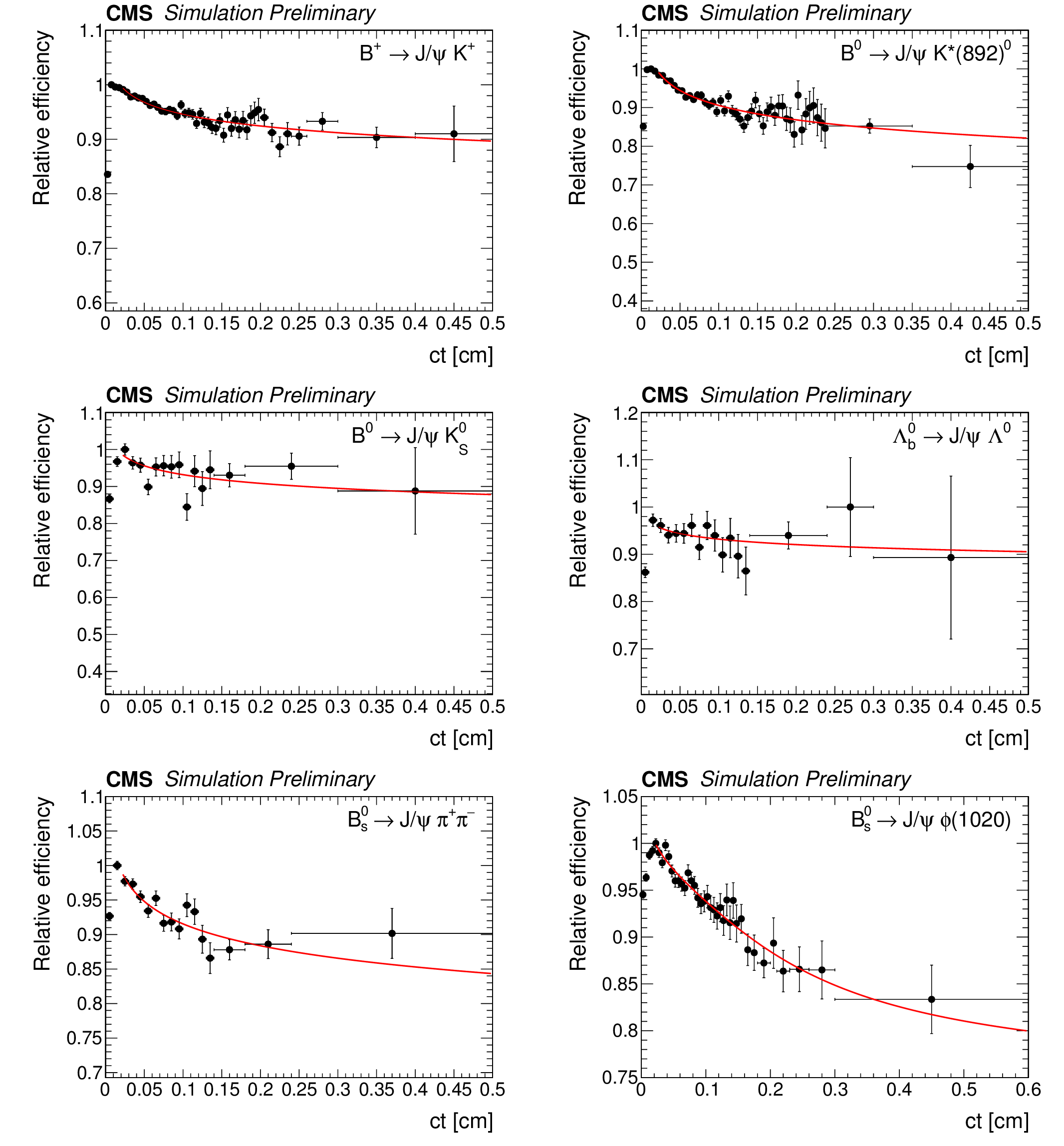
Figure 1:
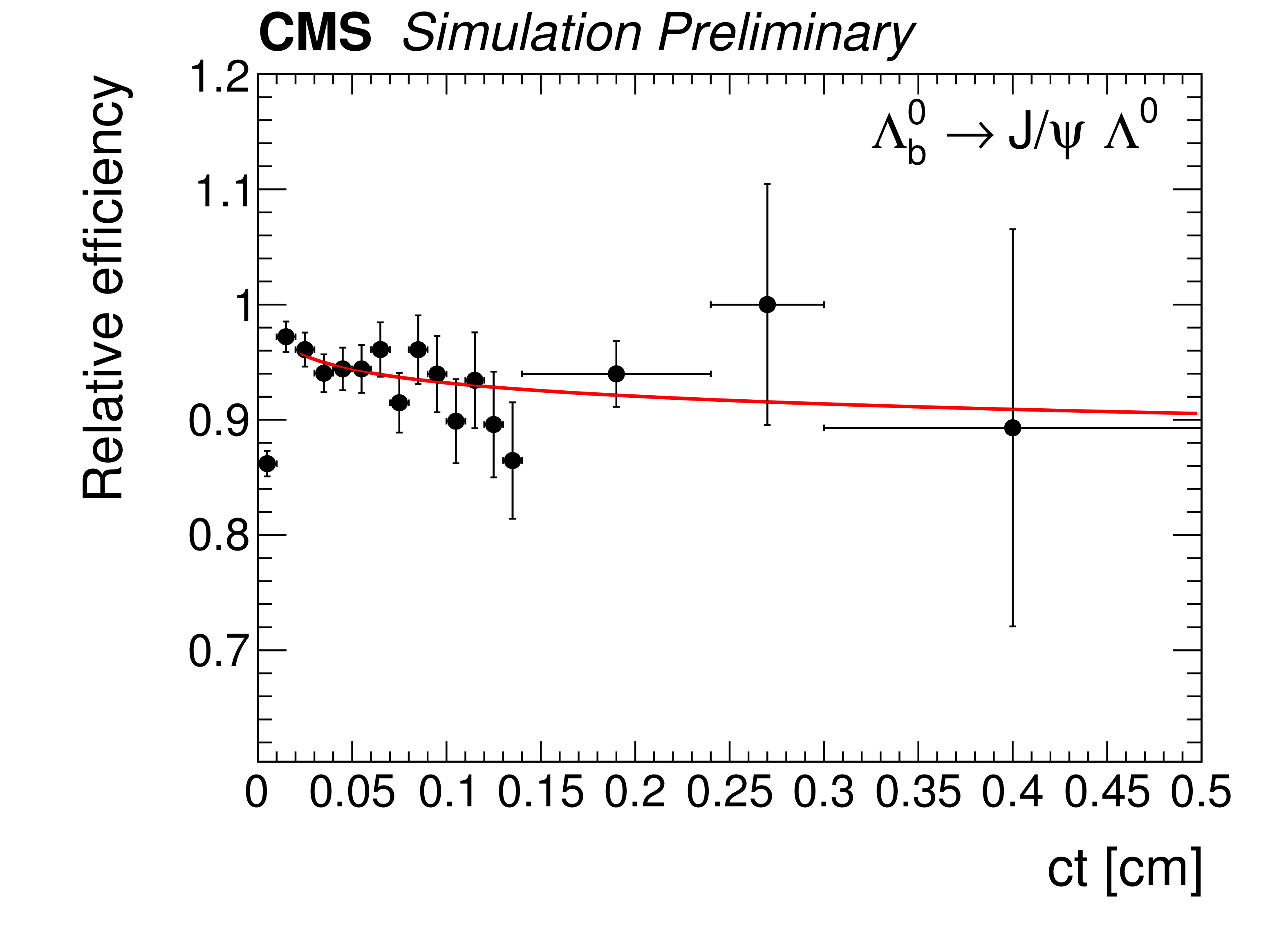
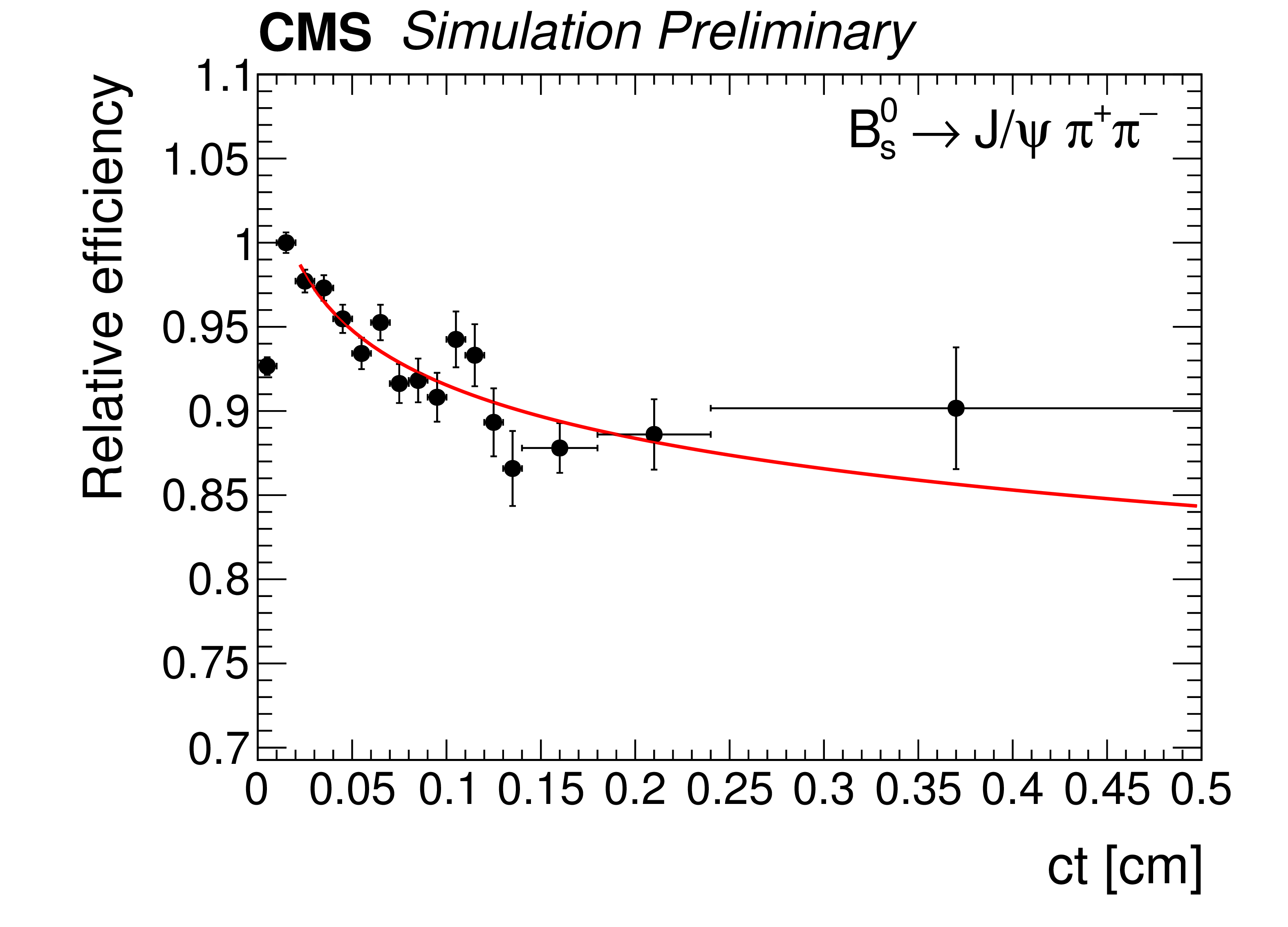
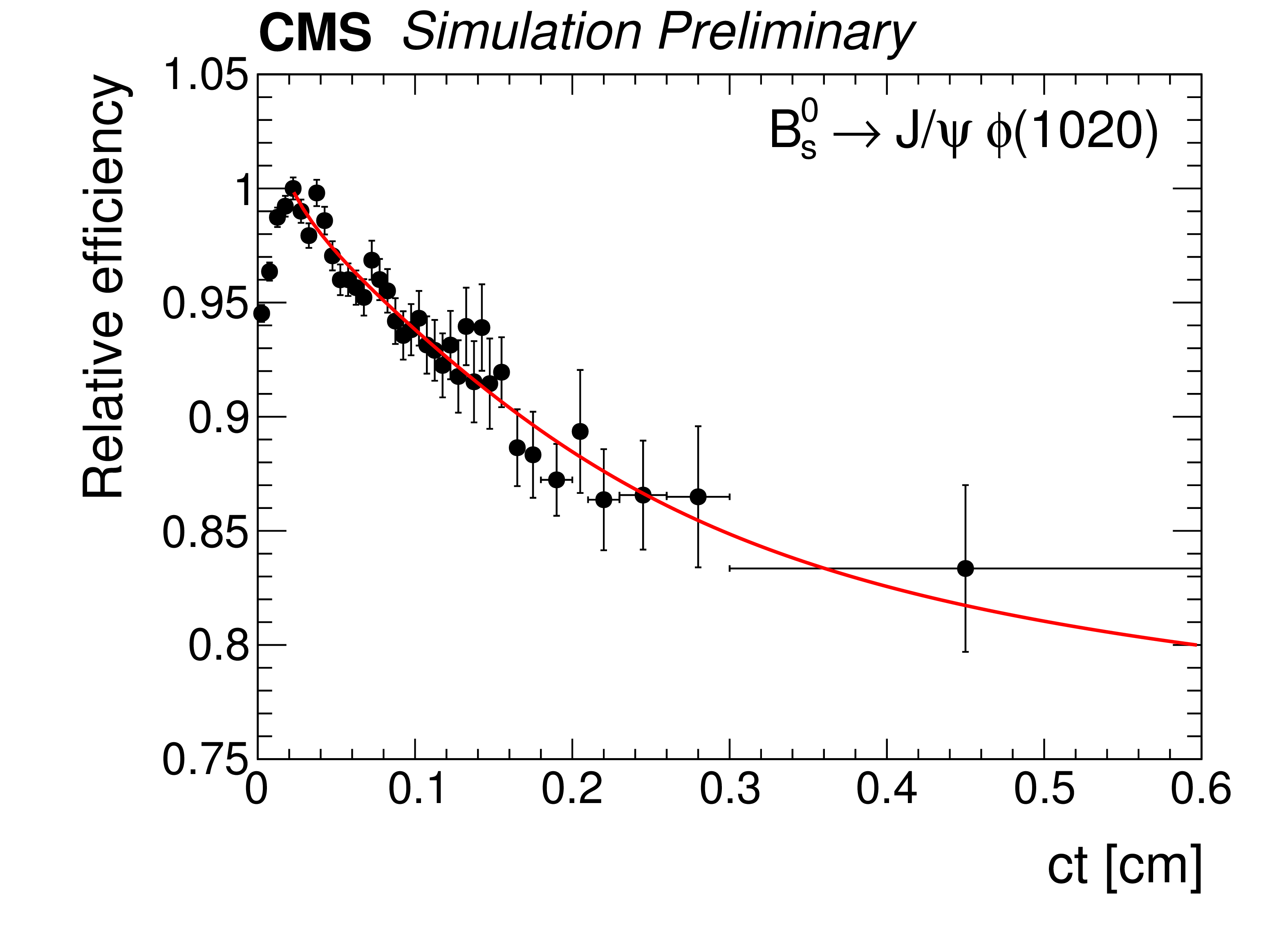
Efficiency versus $ct$ with a superimposed fit to a inverse power function for $ \mathrm{B}^{+} $ (top left), $\mathrm{B}^0 \to \mathrm{J}/\psi\, \mathrm{K}^{*0} $ (top right), $\mathrm{B}^0 \to \mathrm{J}/\psi\, \mathrm{K}_{s}^{0} $ (center left), $ \Lambda^{0}_\mathrm {b}$ (center right), $ \mathrm{B}^0_{s} \to \mathrm{J}/\psi\, \pi^{+} \pi^{-} $ (bottom left), and $ \mathrm{B}^0_{s} \to \mathrm{J}/\psi\, \phi(1020) $ (bottom right). The efficiency scale is arbitrary. |
png pdf |
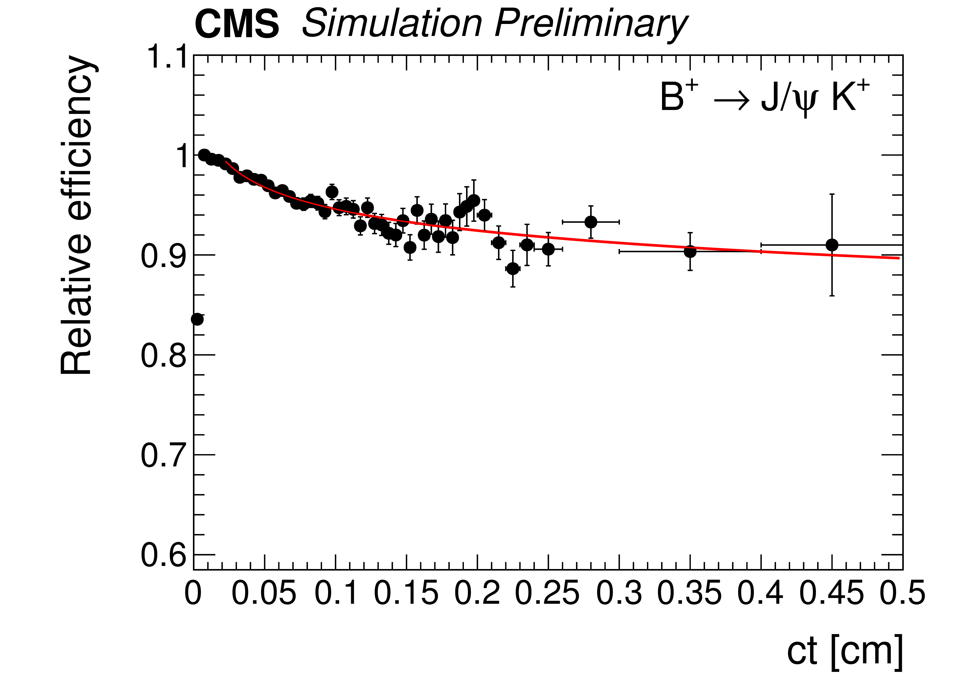
Figure 1-a:
Efficiency versus $ct$ with a superimposed fit to a inverse power function for $ \mathrm{B}^{+} $. The efficiency scale is arbitrary. |
png pdf |
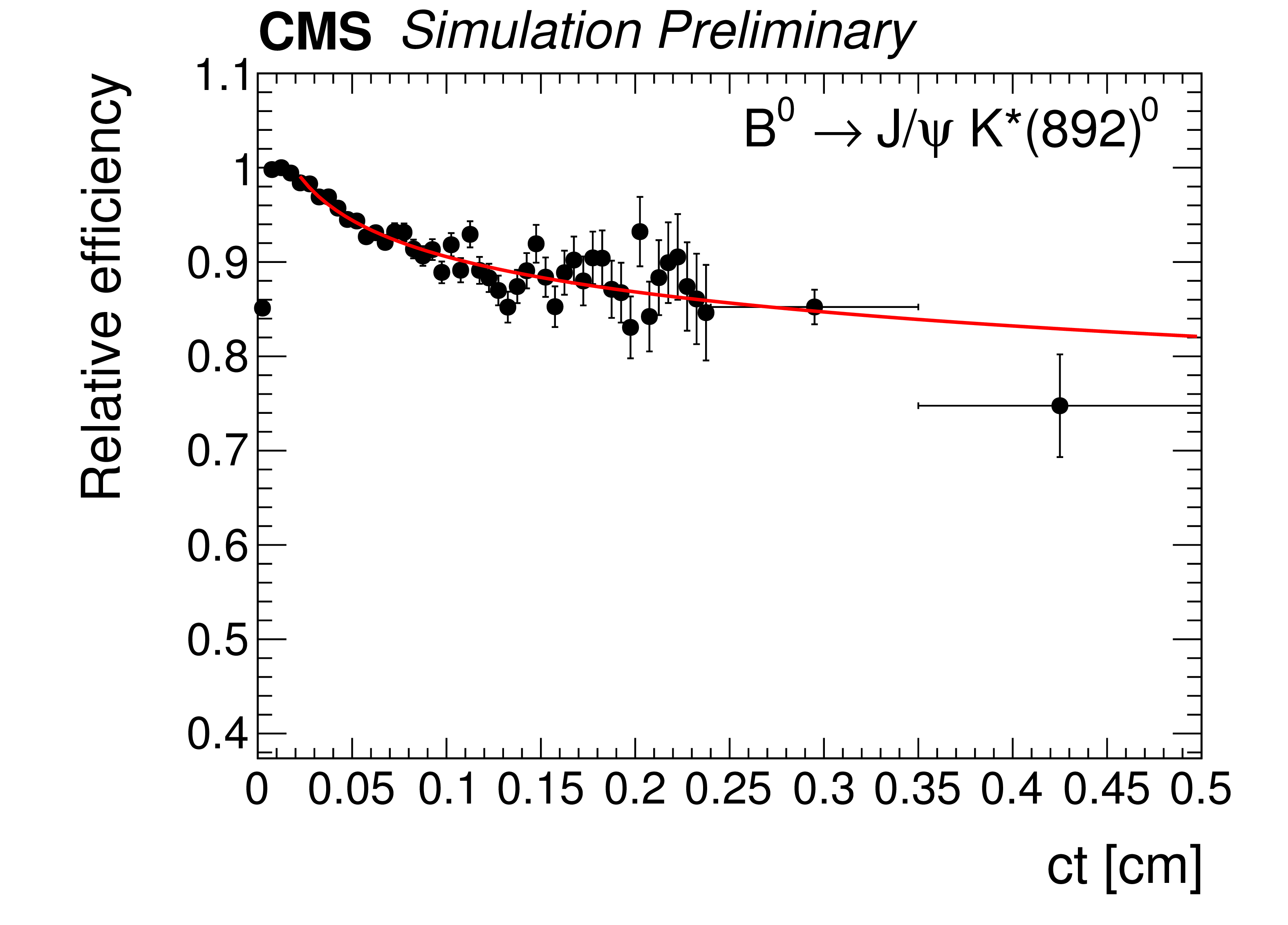
Figure 1-b:
Efficiency versus $ct$ with a superimposed fit to a inverse power function for $\mathrm{B}^0 \to \mathrm{J}/\psi\, \mathrm{K}^{*0} $. The efficiency scale is arbitrary. |
png pdf |
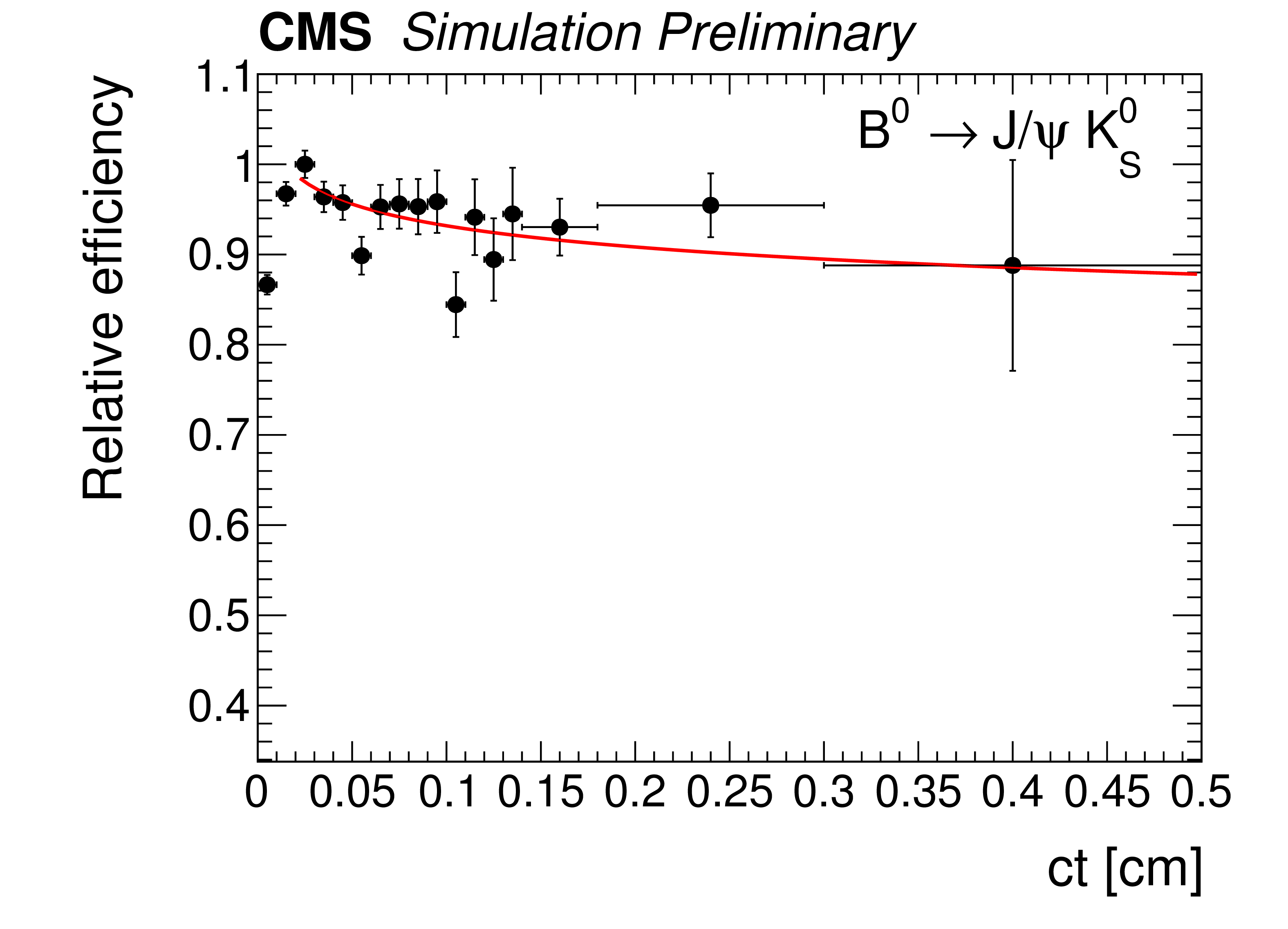
Figure 1-c:
Efficiency versus $ct$ with a superimposed fit to a inverse power function for $\mathrm{B}^0 \to \mathrm{J}/\psi\, \mathrm{K}_{s}^{0} $. The efficiency scale is arbitrary. |
png pdf |
Figure 1-d:
Efficiency versus $ct$ with a superimposed fit to a inverse power function for $ \Lambda^{0}_\mathrm {b}$. The efficiency scale is arbitrary. |
png pdf |
Figure 1-e:
Efficiency versus $ct$ with a superimposed fit to a inverse power function for $ \mathrm{B}^0_{s} \to \mathrm{J}/\psi\, \pi^{+} \pi^{-} $. The efficiency scale is arbitrary. |
png pdf |
Figure 1-f:
Efficiency versus $ct$ with a superimposed fit to a inverse power function for $ \mathrm{B}^0_{s} \to \mathrm{J}/\psi\, \phi(1020) $. The efficiency scale is arbitrary. |
png pdf |
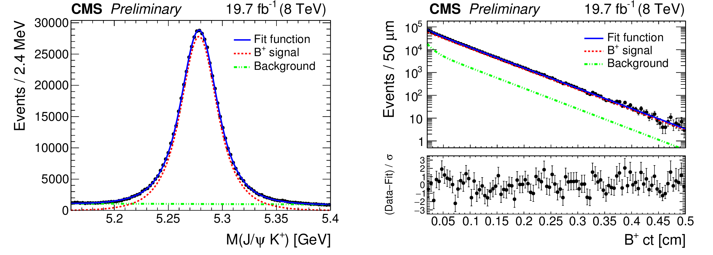
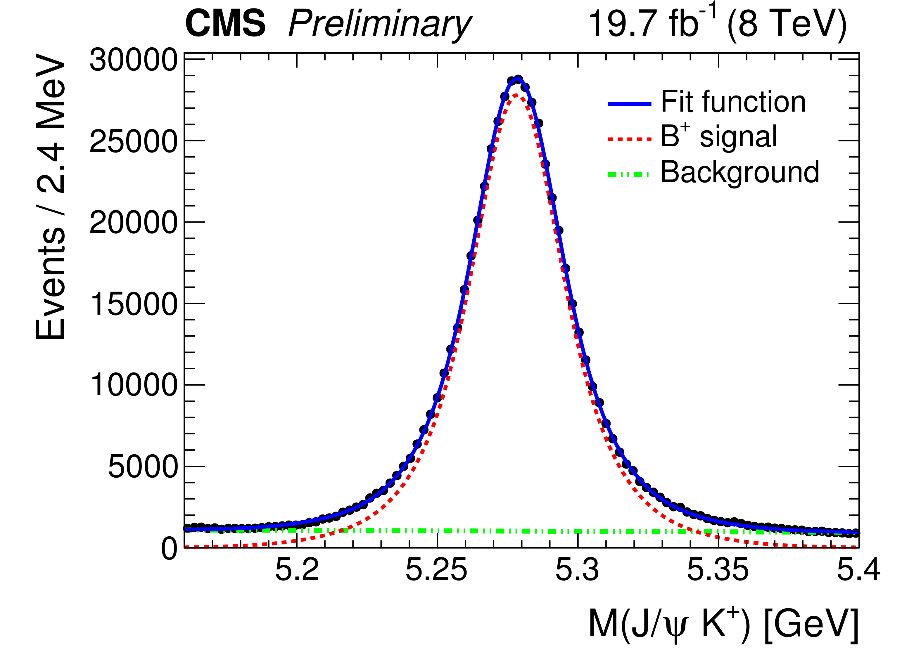
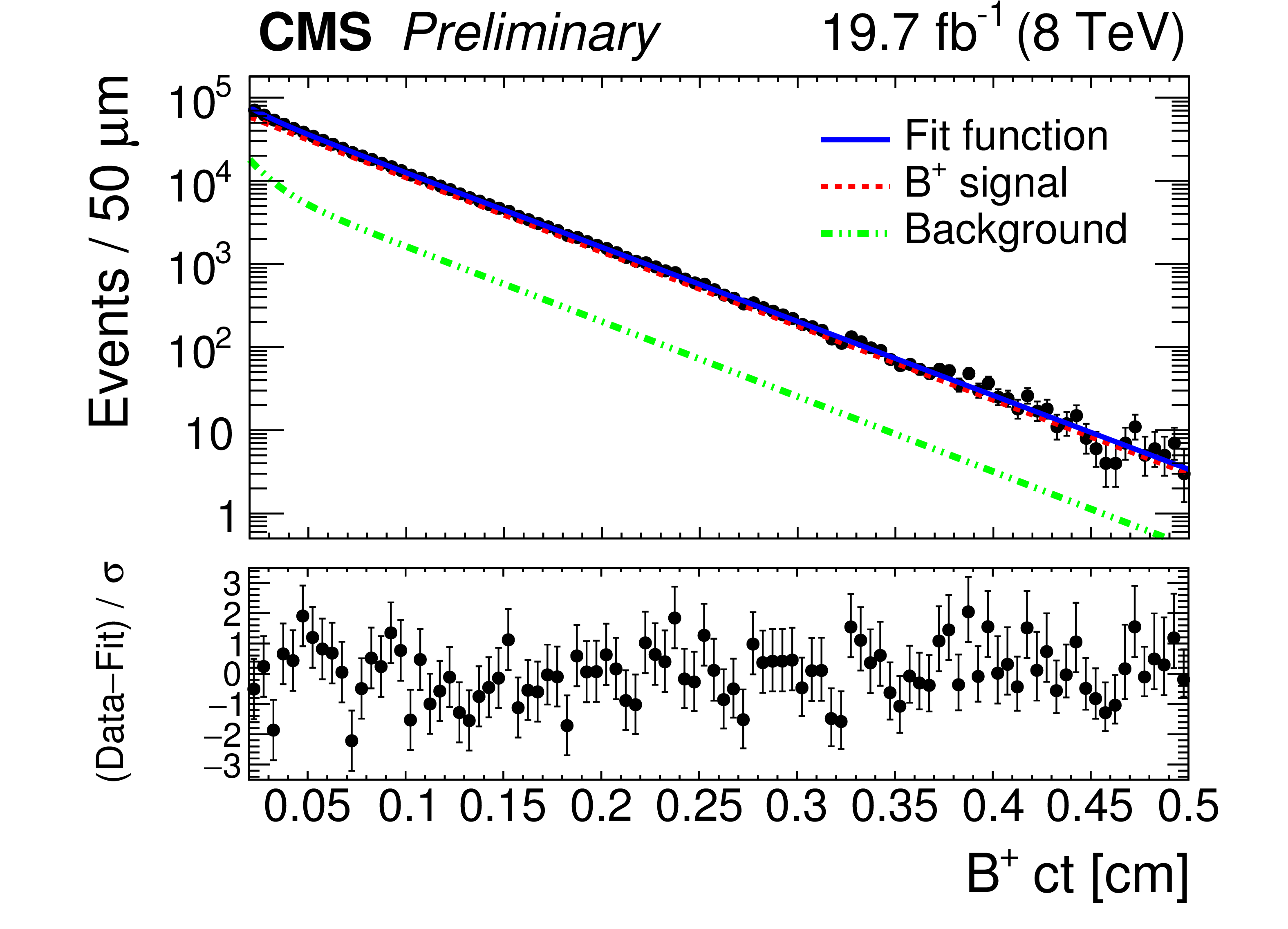
Figure 2:
Invariant mass (left) and $ct$ (right) distributions for $ \mathrm{B}^{+} $ candidates. The curves are projections of the maximum-likelihood fit to the data, with the contributions from signal (dashed), background (dotted), and the sum of signal and background (solid) shown. The bottom panel of the right figure shows the difference between the observed data and the fit divided by the data uncertainty. |
png pdf |
Figure 2-a:
Invariant mass distribution for $ \mathrm{B}^{+} $ candidates. The curves are projections of the maximum-likelihood fit to the data, with the contributions from signal (dashed), background (dotted), and the sum of signal and background (solid) shown. |
png pdf |
Figure 2-b:
$ct$ distribution for $ \mathrm{B}^{+} $ candidates. The curves are projections of the maximum-likelihood fit to the data, with the contributions from signal (dashed), background (dotted), and the sum of signal and background (solid) shown. The bottom panel shows the difference between the observed data and the fit divided by the data uncertainty. |
png pdf |
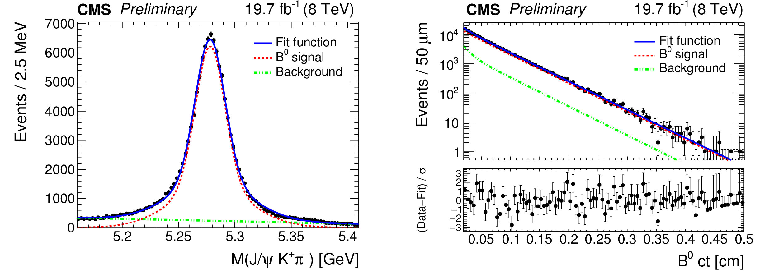
Figure 3:
Invariant mass (left) and $ct$ (right) distributions for $ {\mathrm{B}^0 } $ candidates reconstructed from $\mathrm{J}/\psi\, \mathrm{K}^{*0} $ decays. The curves are projections of the maximum-likelihood fit to the data, with the contributions from signal (dashed), background (dotted), and the sum of signal and background (solid) shown. The bottom panel of the right figure shows the difference between the observed data and the fit divided by the data uncertainty. |
png pdf |
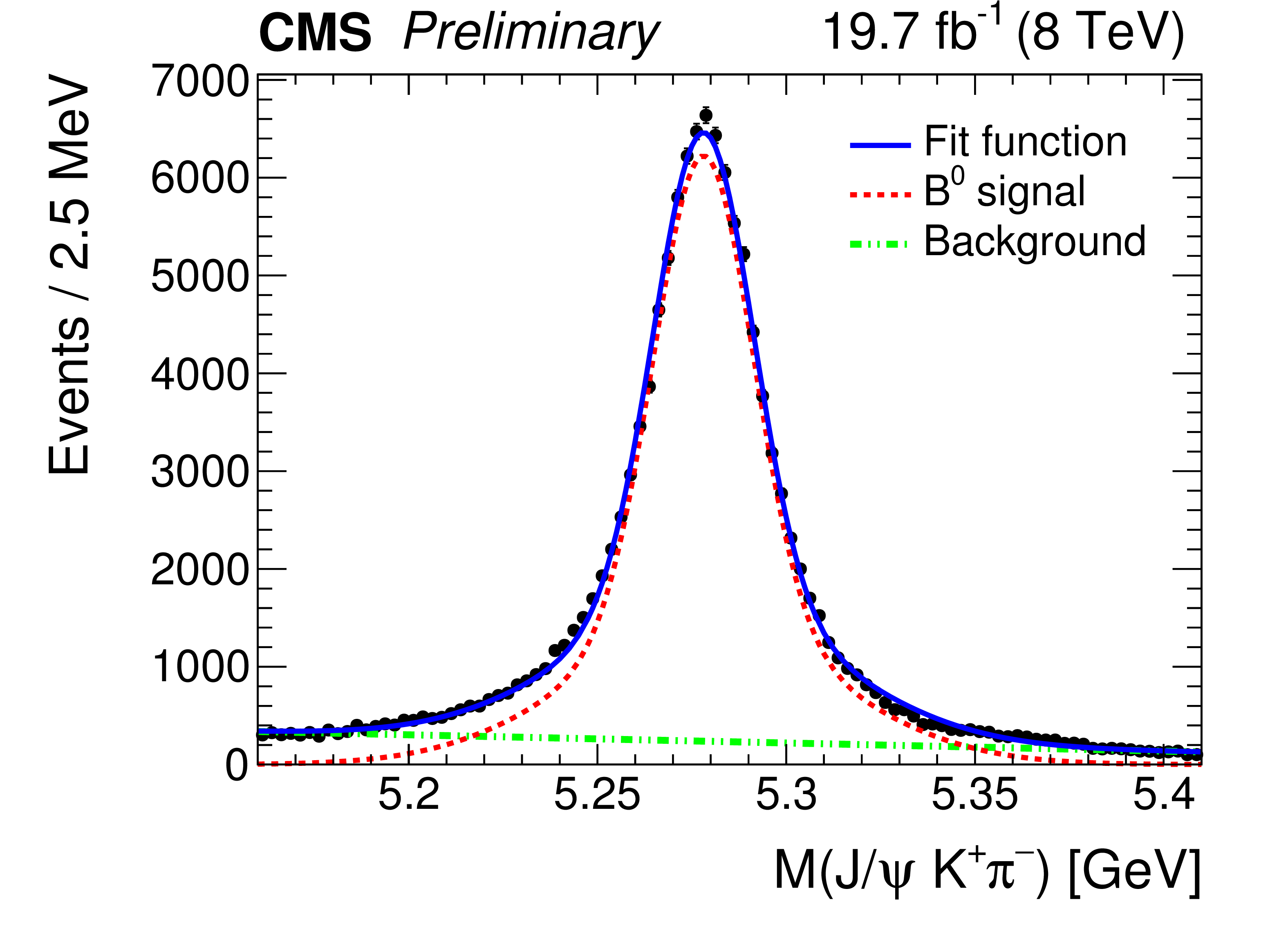
Figure 3-a:
Invariant mass distribution for $ {\mathrm{B}^0 } $ candidates reconstructed from $\mathrm{J}/\psi\, \mathrm{K}^{*0} $ decays. The curves are projections of the maximum-likelihood fit to the data, with the contributions from signal (dashed), background (dotted), and the sum of signal and background (solid) shown. |
png pdf |
Figure 3-b:
$ct$ distribution for $ {\mathrm{B}^0 } $ candidates reconstructed from $\mathrm{J}/\psi\, \mathrm{K}^{*0} $ decays. The curves are projections of the maximum-likelihood fit to the data, with the contributions from signal (dashed), background (dotted), and the sum of signal and background (solid) shown. |
png pdf |
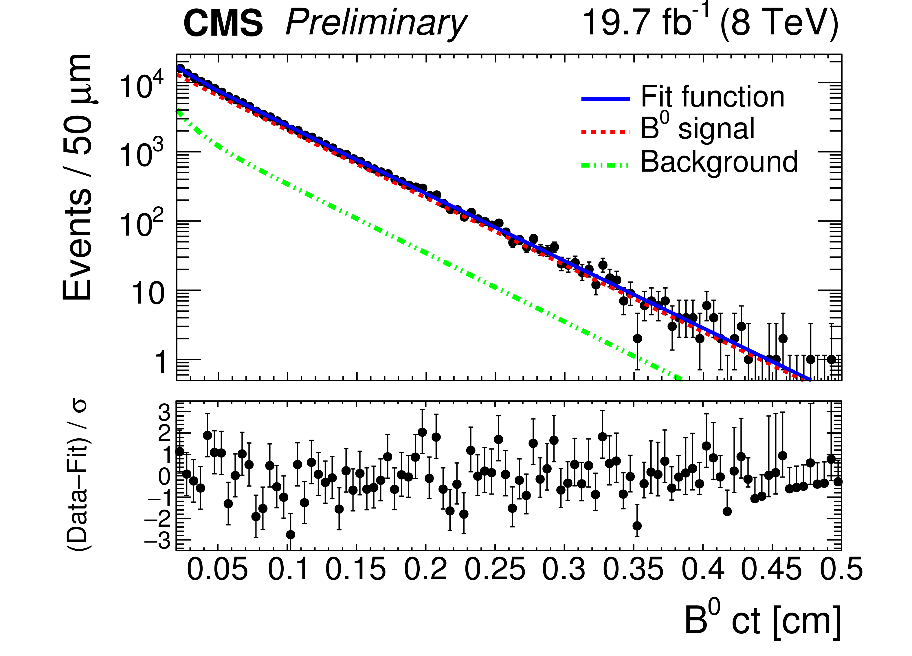
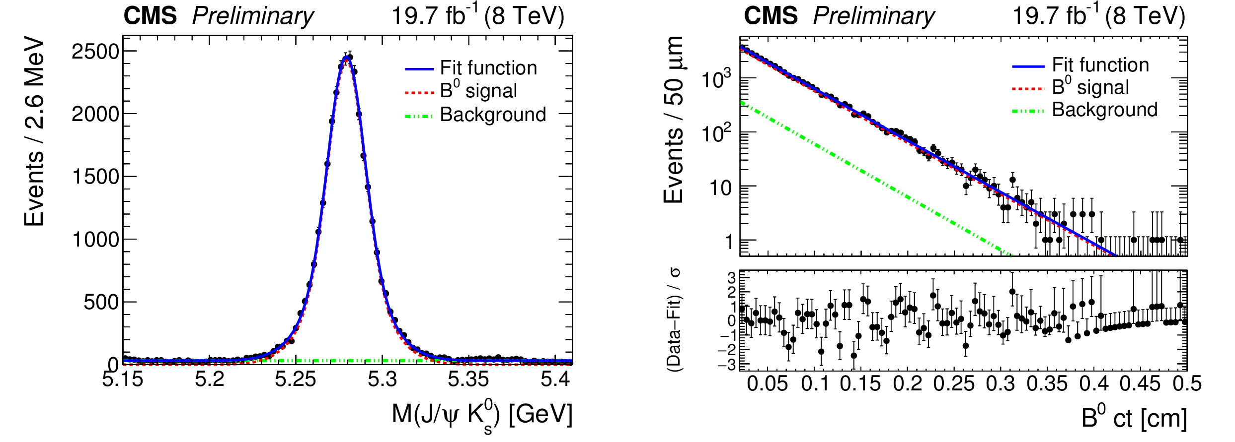
Figure 4:
Invariant mass (left) and $ct$ (right) distributions for $ {\mathrm{B}^0 } $ candidates reconstructed from $ \mathrm{J}/\psi\, \mathrm{K}_{s}^{0} $ decays. The curves are projections of the maximum-likelihood fit to the data, with the contributions from signal (dashed), background (dotted), and the sum of signal and background (solid) shown. The bottom panel of the right figure shows the difference between the observed data and the fit divided by the data uncertainty. |
png pdf |
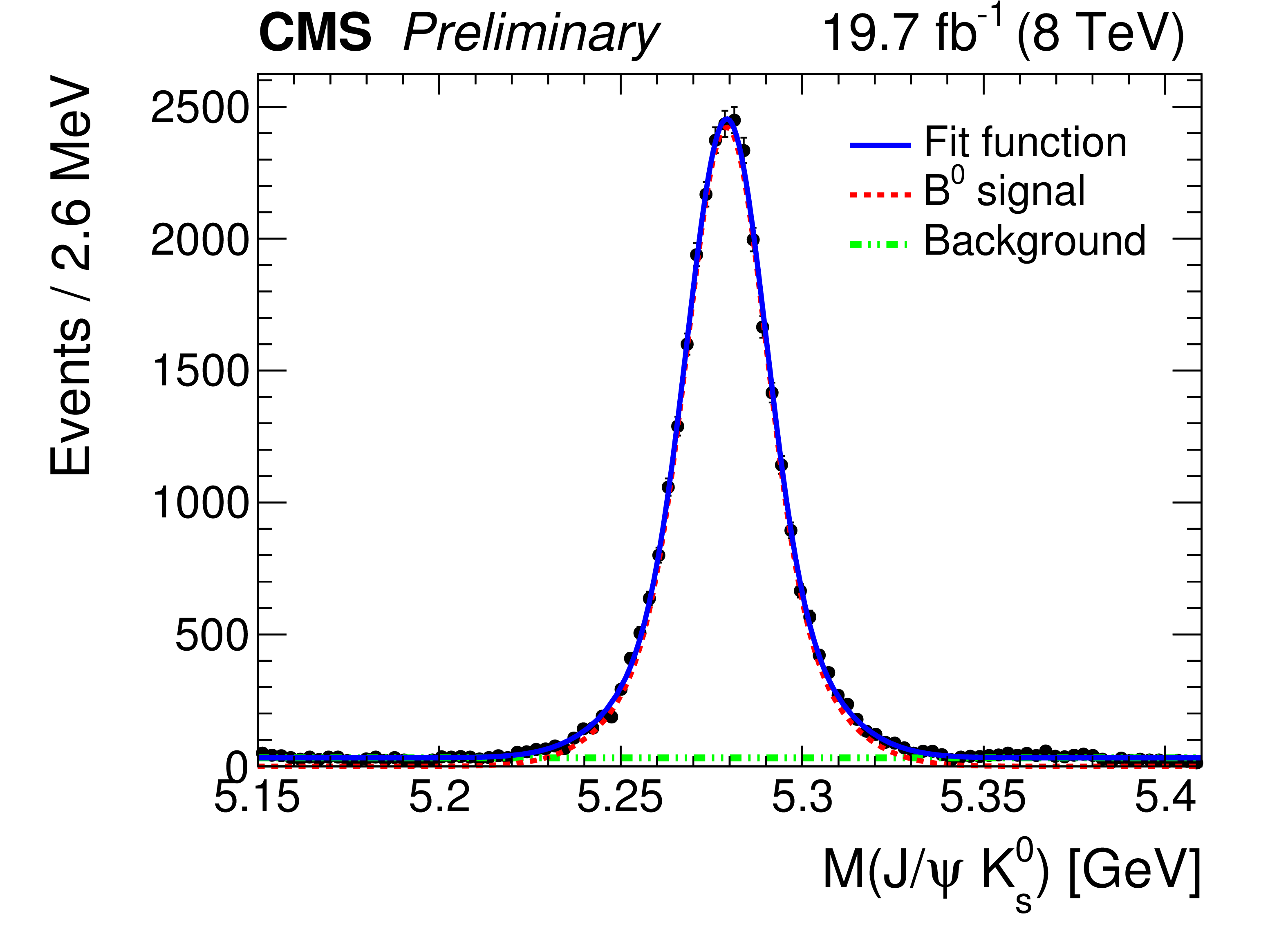
Figure 4-a:
Invariant mass distribution for $ {\mathrm{B}^0 } $ candidates reconstructed from $ \mathrm{J}/\psi\, \mathrm{K}_{s}^{0} $ decays. The curves are projections of the maximum-likelihood fit to the data, with the contributions from signal (dashed), background (dotted), and the sum of signal and background (solid) shown. |
png pdf |
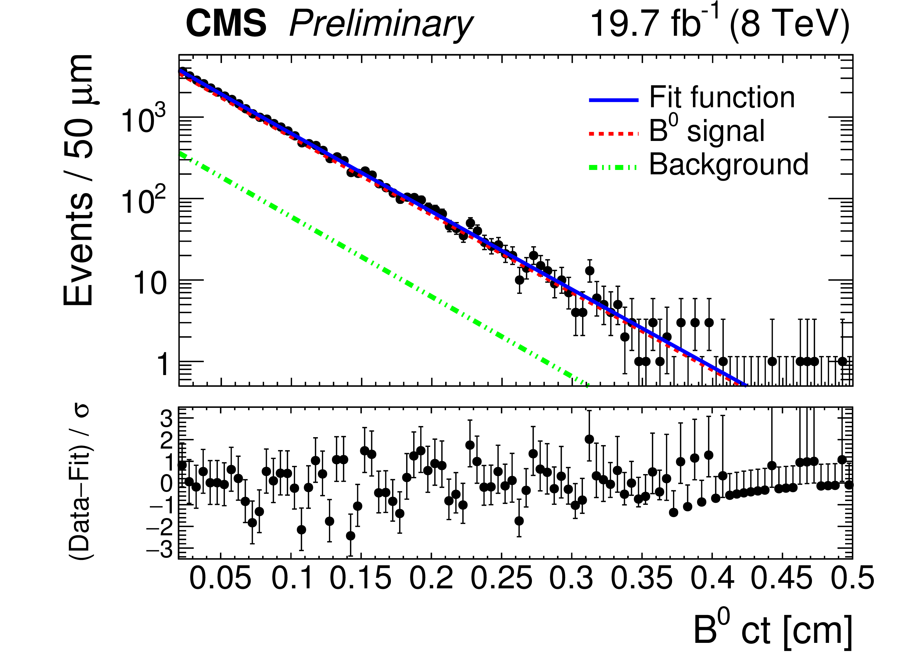
Figure 4-b:
$ct$ distribution for $ {\mathrm{B}^0 } $ candidates reconstructed from $ \mathrm{J}/\psi\, \mathrm{K}_{s}^{0} $ decays. The curves are projections of the maximum-likelihood fit to the data, with the contributions from signal (dashed), background (dotted), and the sum of signal and background (solid) shown. The bottom panel of the right figure shows the difference between the observed data and the fit divided by the data uncertainty. |
png pdf |
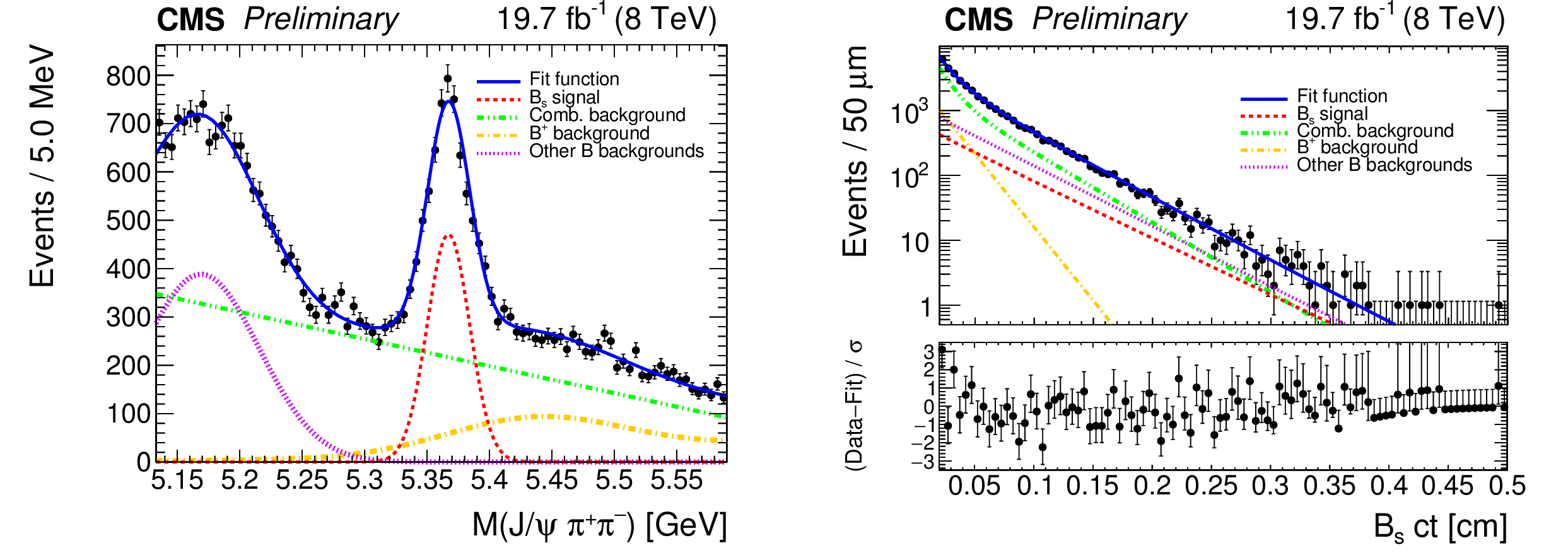
Figure 5:
Invariant mass (left) and $ct$ (right) distributions for $ \mathrm{B}^0_{s} $ candidates reconstructed from $\mathrm{J}/\psi\, \pi^{+} \pi^{-} $ decays. The curves are projections of the maximum-likelihood fit to the data, with the contributions from signal (dashed), combinatorial background (dotted), misidentified $\mathrm{B}^{+} \to \mathrm{J}/\psi\, \mathrm{K}^{+} $ background (dashed-dotted), partially reconstructed and (other) misidentified B backgrounds (vertical dashed), and the sum of signal and backgrounds (solid) shown. The bottom panel of the right figure shows the difference between the observed data and the fit divided by the data uncertainty. |
png pdf |
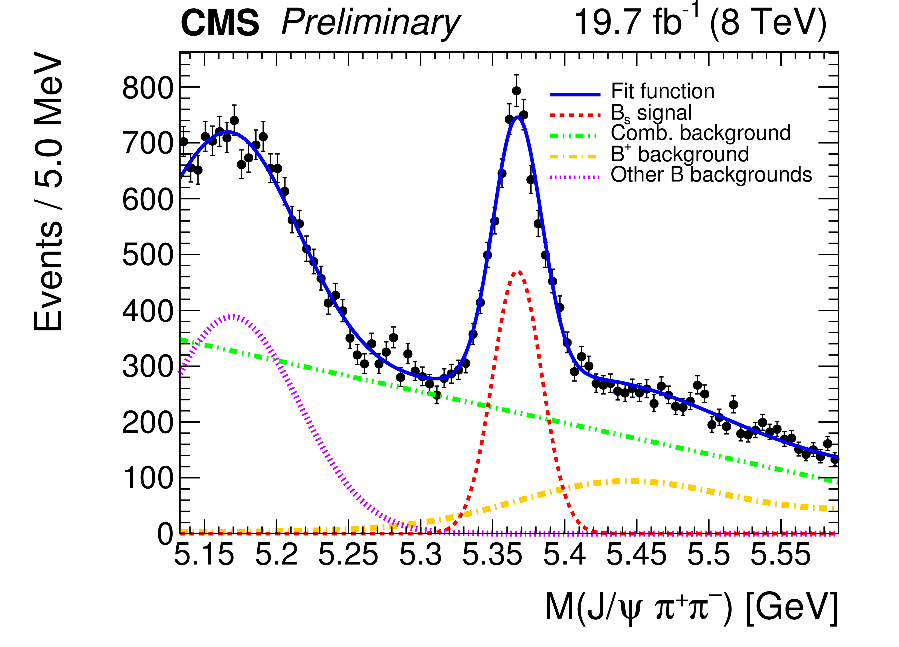
Figure 5-a:
Invariant mass distribution for $ \mathrm{B}^0_{s} $ candidates reconstructed from $\mathrm{J}/\psi\, \pi^{+} \pi^{-} $ decays. The curves are projections of the maximum-likelihood fit to the data, with the contributions from signal (dashed), combinatorial background (dotted), misidentified $\mathrm{B}^{+} \to \mathrm{J}/\psi\, \mathrm{K}^{+} $ background (dashed-dotted), partially reconstructed and (other) misidentified B backgrounds (vertical dashed), and the sum of signal and backgrounds (solid) shown. |
png pdf |
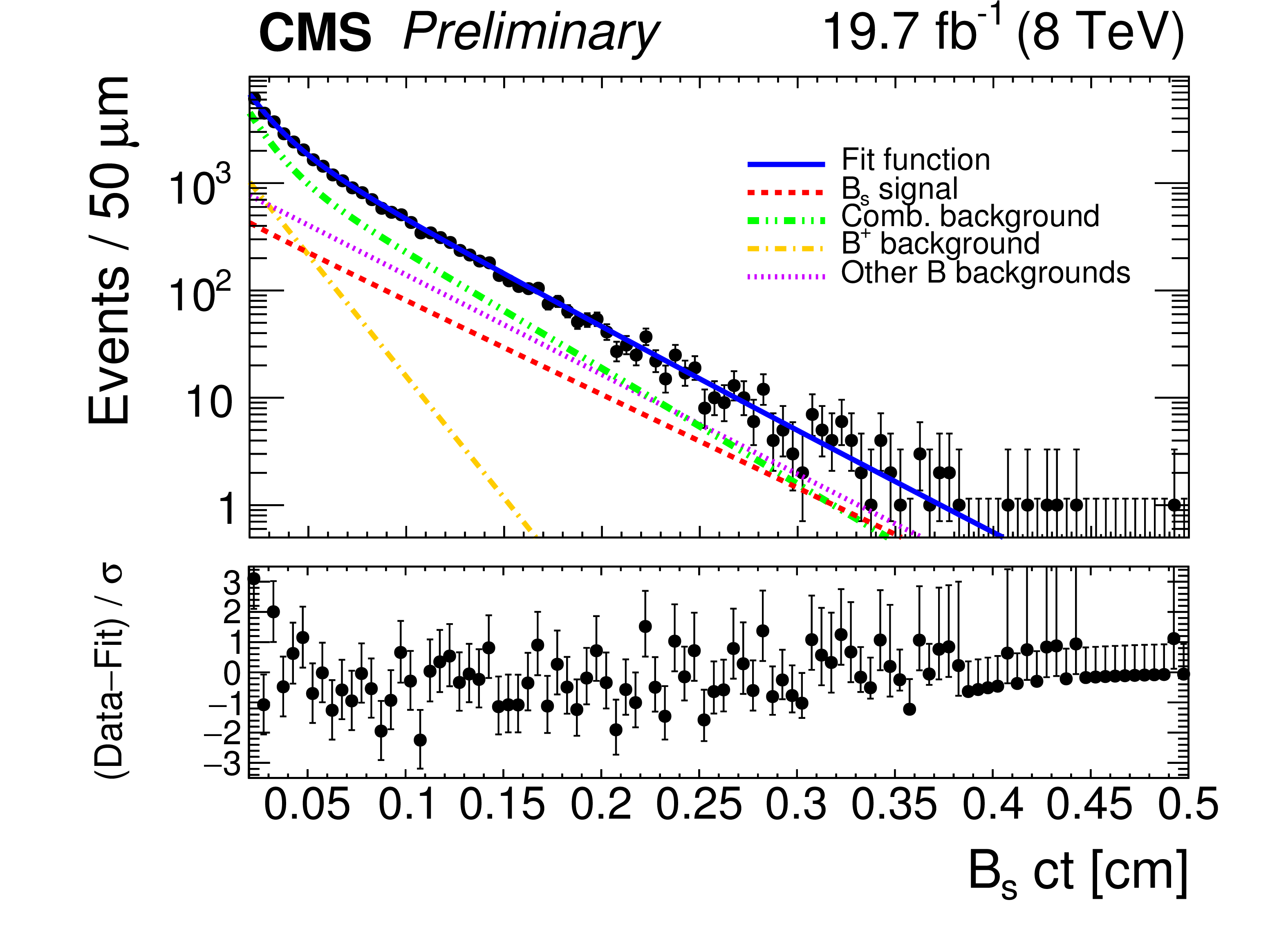
Figure 5-b:
$ct$ distribution for $ \mathrm{B}^0_{s} $ candidates reconstructed from $\mathrm{J}/\psi\, \pi^{+} \pi^{-} $ decays. The curves are projections of the maximum-likelihood fit to the data, with the contributions from signal (dashed), combinatorial background (dotted), misidentified $\mathrm{B}^{+} \to \mathrm{J}/\psi\, \mathrm{K}^{+} $ background (dashed-dotted), partially reconstructed and (other) misidentified B backgrounds (vertical dashed), and the sum of signal and backgrounds (solid) shown. The bottom panel of the right figure shows the difference between the observed data and the fit divided by the data uncertainty. |

png pdf |
Figure 6:
Invariant mass (left) and $ct$ (right) distributions for $ \mathrm{B}^0_{s} $ candidates reconstructed from $\mathrm{J}/\psi\, \phi {1020} $ decays. The curves are projections of the maximum-likelihood fit to the data, with the contributions from signal (dashed), background (dotted), and the sum of signal and background (solid) shown. The bottom panel of the right figure shows the difference between the observed data and the fit divided by the data uncertainty. |
png pdf |
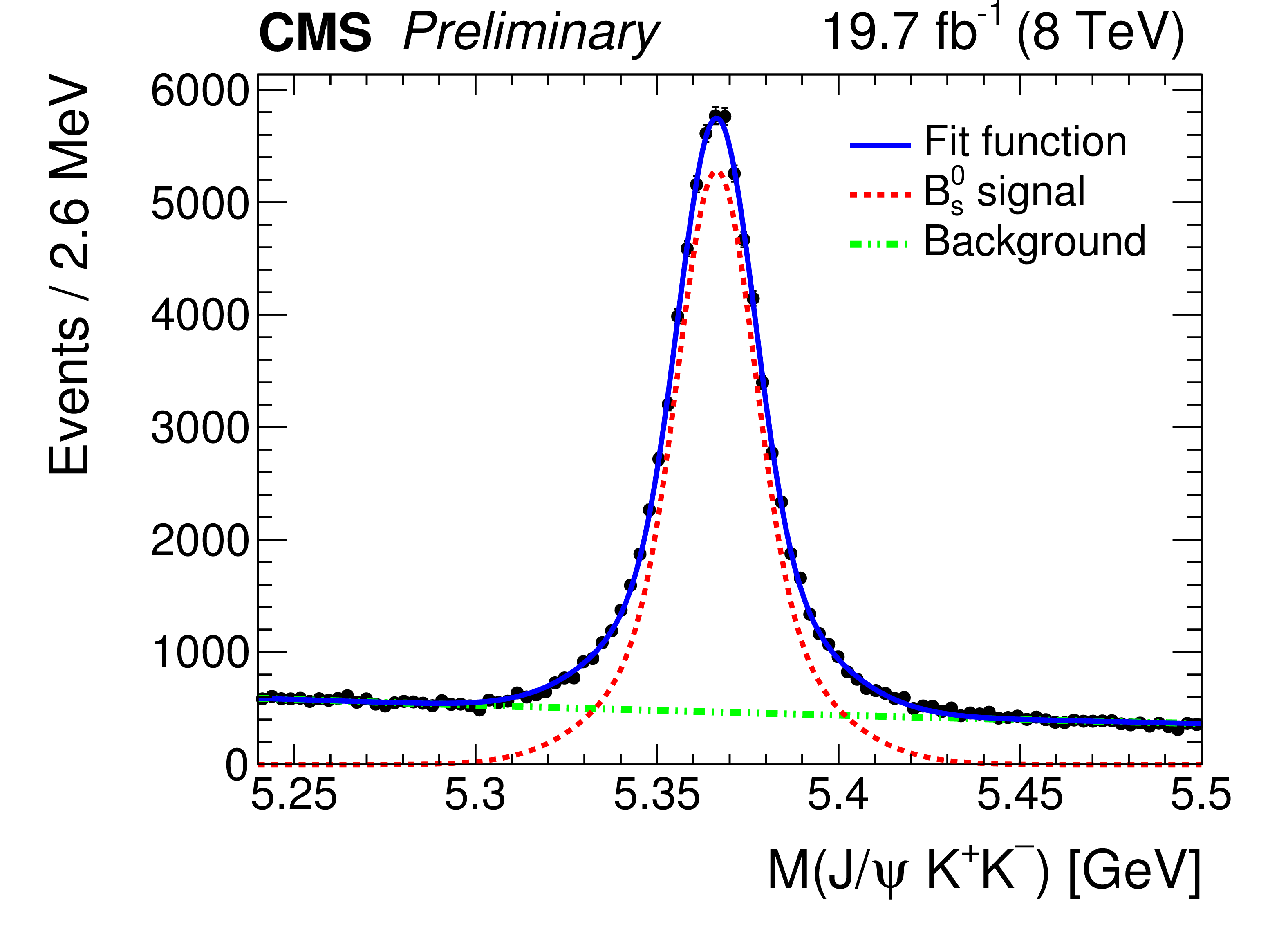
Figure 6-a:
Invariant mass distribution for $ \mathrm{B}^0_{s} $ candidates reconstructed from $\mathrm{J}/\psi\, \phi {1020} $ decays. The curves are projections of the maximum-likelihood fit to the data, with the contributions from signal (dashed), background (dotted), and the sum of signal and background (solid) shown. |
png pdf |
Figure 6-b:
$ct$ distribution for $ \mathrm{B}^0_{s} $ candidates reconstructed from $\mathrm{J}/\psi\, \phi {1020} $ decays. The curves are projections of the maximum-likelihood fit to the data, with the contributions from signal (dashed), background (dotted), and the sum of signal and background (solid) shown. The bottom panel of the right figure shows the difference between the observed data and the fit divided by the data uncertainty. |
png pdf |
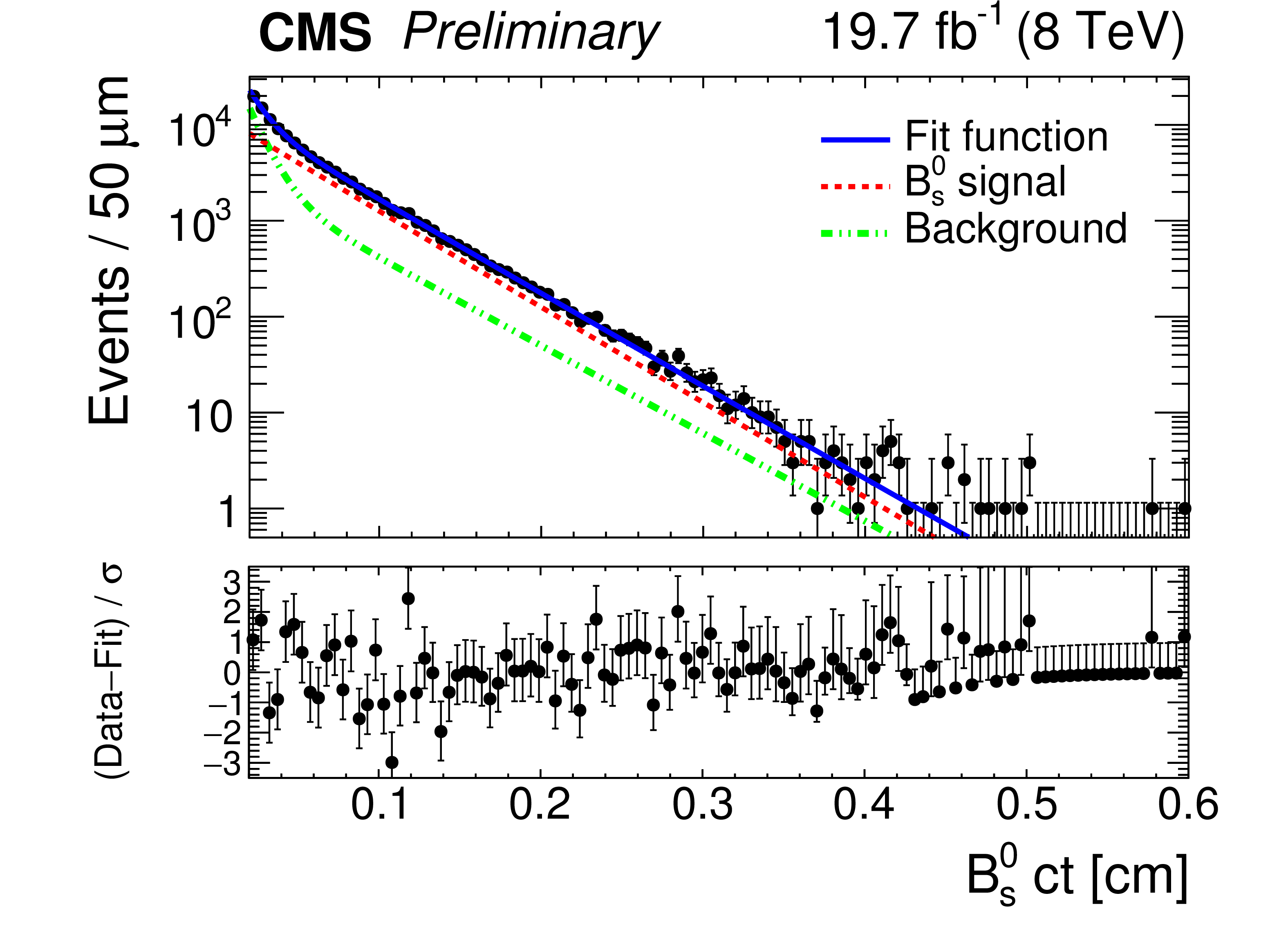
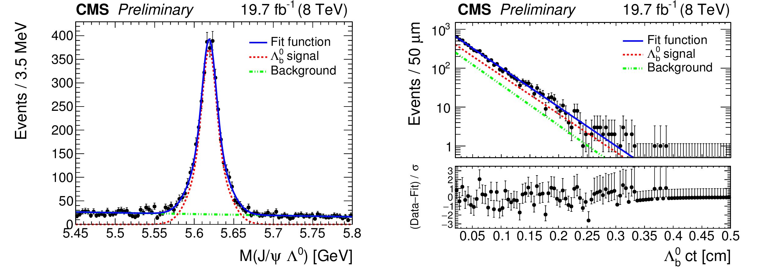
Figure 7:
Invariant mass (left) and $ct$ (right) distributions for $\Lambda^{0}_\mathrm {b}$ candidates. The curves are projections of the maximum-likelihood fit to the data, with the contributions from signal (dashed), background (dotted), and the sum of signal and background (solid) shown.The bottom panel of the right figure shows the difference between the observed data and the fit divided by the data uncertainty. |
png pdf |
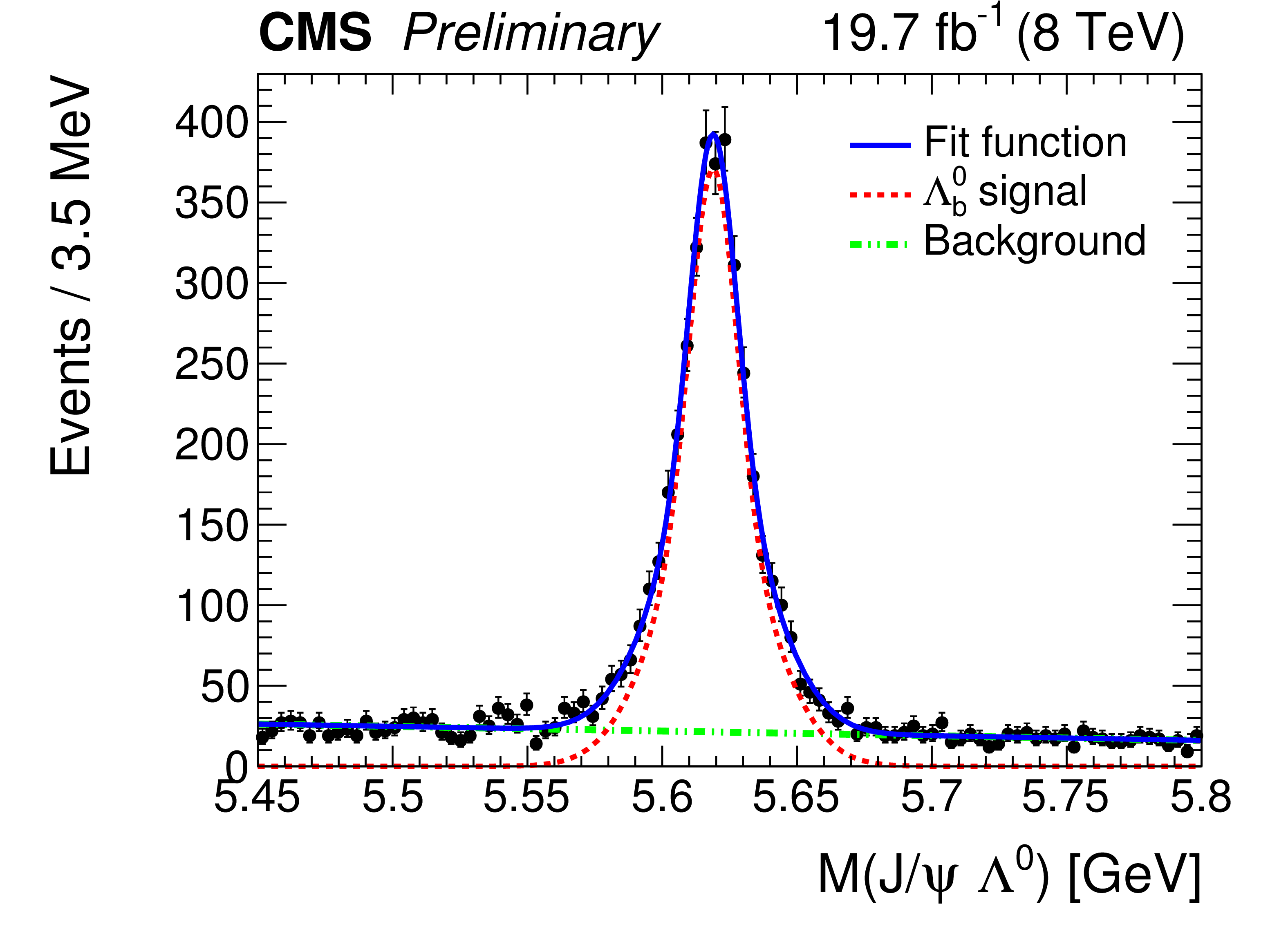
Figure 7-a:
Invariant mass distribution for $\Lambda^{0}_\mathrm {b}$ candidates. The curves are projections of the maximum-likelihood fit to the data, with the contributions from signal (dashed), background (dotted), and the sum of signal and background (solid) shown. |
png pdf |
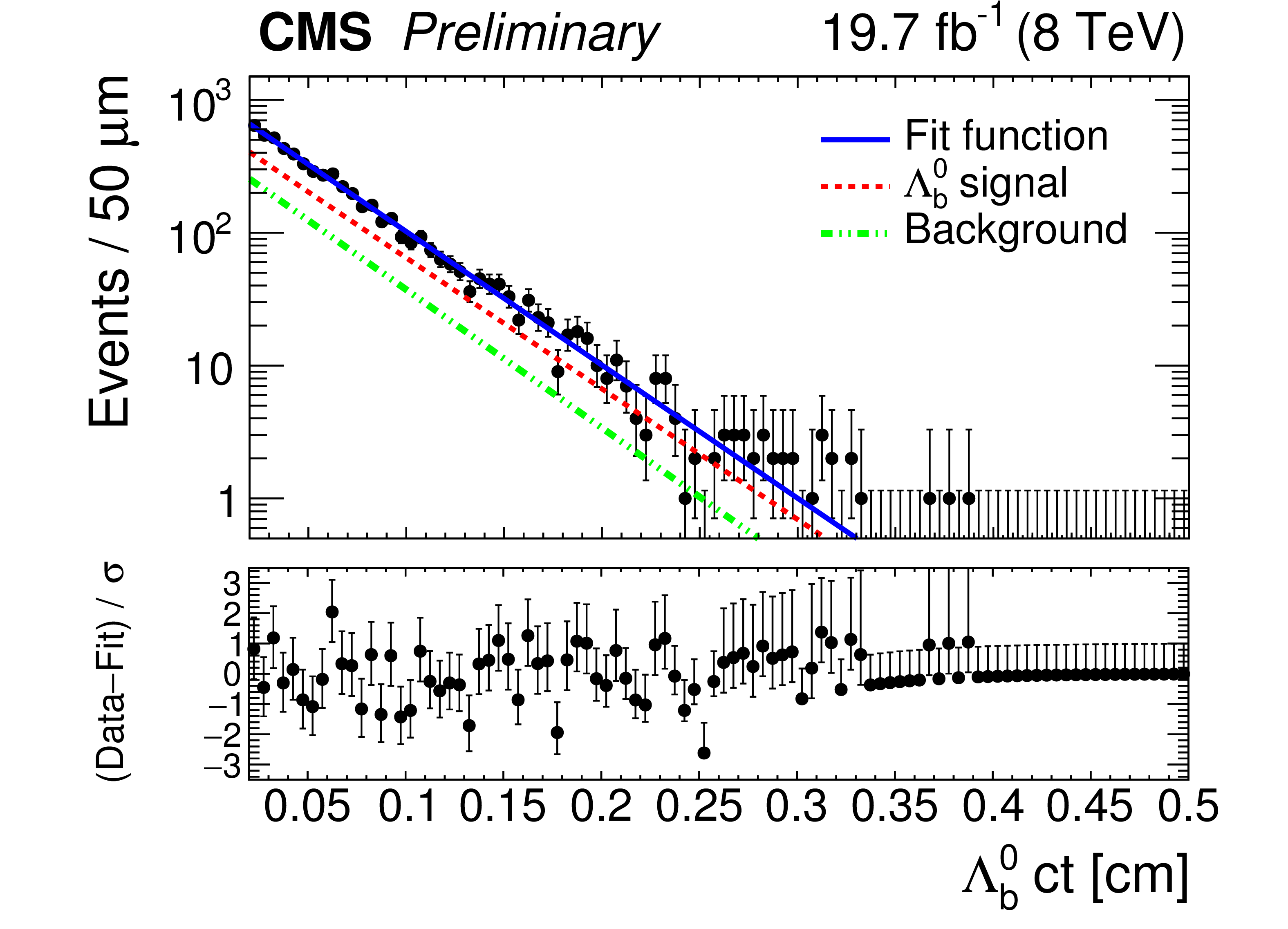
Figure 7-b:
$ct$ distribution for $\Lambda^{0}_\mathrm {b}$ candidates. The curves are projections of the maximum-likelihood fit to the data, with the contributions from signal (dashed), background (dotted), and the sum of signal and background (solid) shown.The bottom panel of the right figure shows the difference between the observed data and the fit divided by the data uncertainty. |
png pdf |
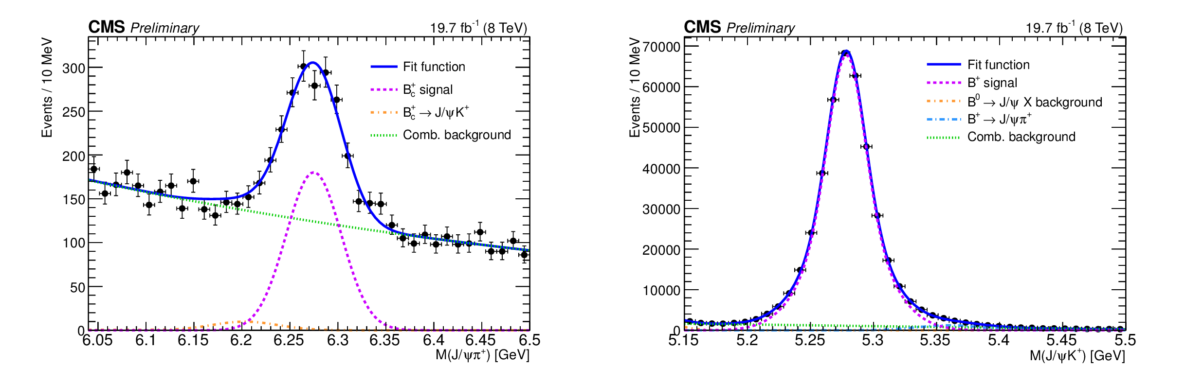
Figure 8:
The $\mathrm{J}/\psi\, \pi^{+} $ invariant mass distribution (left). The solid line represents the signal-plus-background fit. The dashed line represents the signal component, the dotted line the combinatorial background, and the dashed-dotted line the contribution from $\mathrm{B}_{c} \to \mathrm{J}/\psi\, \mathrm{K}^{+} $ decays. The $\mathrm{J}/\psi\, \mathrm{K}^{+} $ invariant mass distribution (right). The result of the fit is superimposed with a solid line. The signal is shown with a dashed line, the dotted-dashed curves represent the $\mathrm{B}^{+} \to {\mathrm{J}/\psi\, } \pi^{+} $ and $\mathrm{B}^0 $ contributions, and the dotted curve the combinatorial background. |
png pdf |
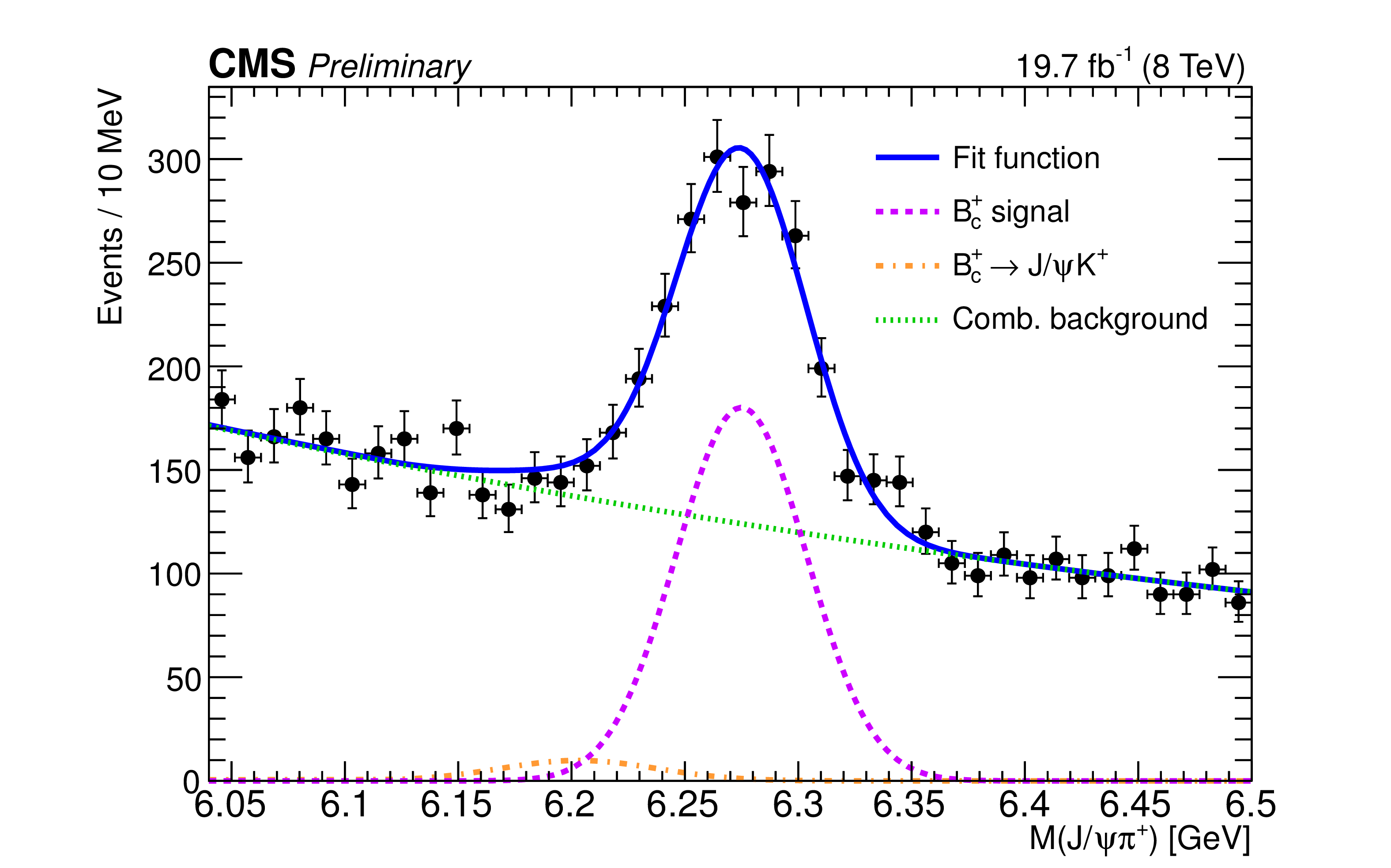
Figure 8-a:
The $\mathrm{J}/\psi\, \pi^{+} $ invariant mass distribution. The solid line represents the signal-plus-background fit. The dashed line represents the signal component, the dotted line the combinatorial background, and the dashed-dotted line the contribution from $\mathrm{B}_{c} \to \mathrm{J}/\psi\, \mathrm{K}^{+} $ decays. |
png pdf |
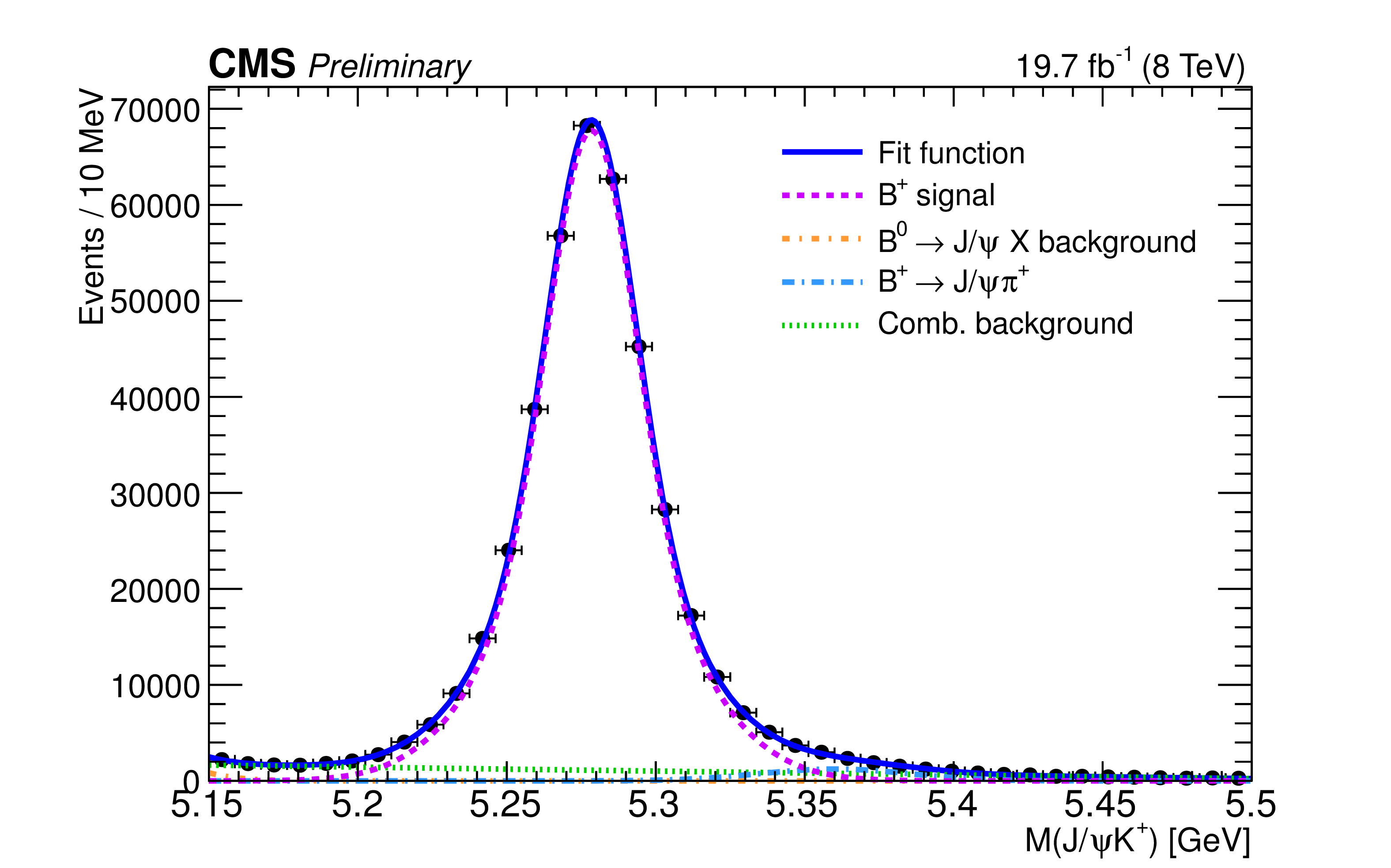
Figure 8-b:
The $\mathrm{J}/\psi\, \mathrm{K}^{+} $ invariant mass distribution. The result of the fit is superimposed with a solid line. The signal is shown with a dashed line, the dotted-dashed curves represent the $\mathrm{B}^{+} \to {\mathrm{J}/\psi\, } \pi^{+} $ and $\mathrm{B}^0 $ contributions, and the dotted curve the combinatorial background. |

png pdf |
Figure 9:
The yield (left) of $\mathrm{B}_{c}^{+} \to \mathrm{J}/\psi\, \pi^{+} $ and $\mathrm{B}^{+} \to \mathrm{J}/\psi\, \mathrm{K}^{+} $ events as a function of $ct$, normalized to the bin width, as determined from fits to the invariant mass distributions. Ratio (right) of the $\mathrm{B}_{c}$ and $\mathrm{B}^{+} $ efficiency distributions as a function of ${ct} $. |
png pdf |
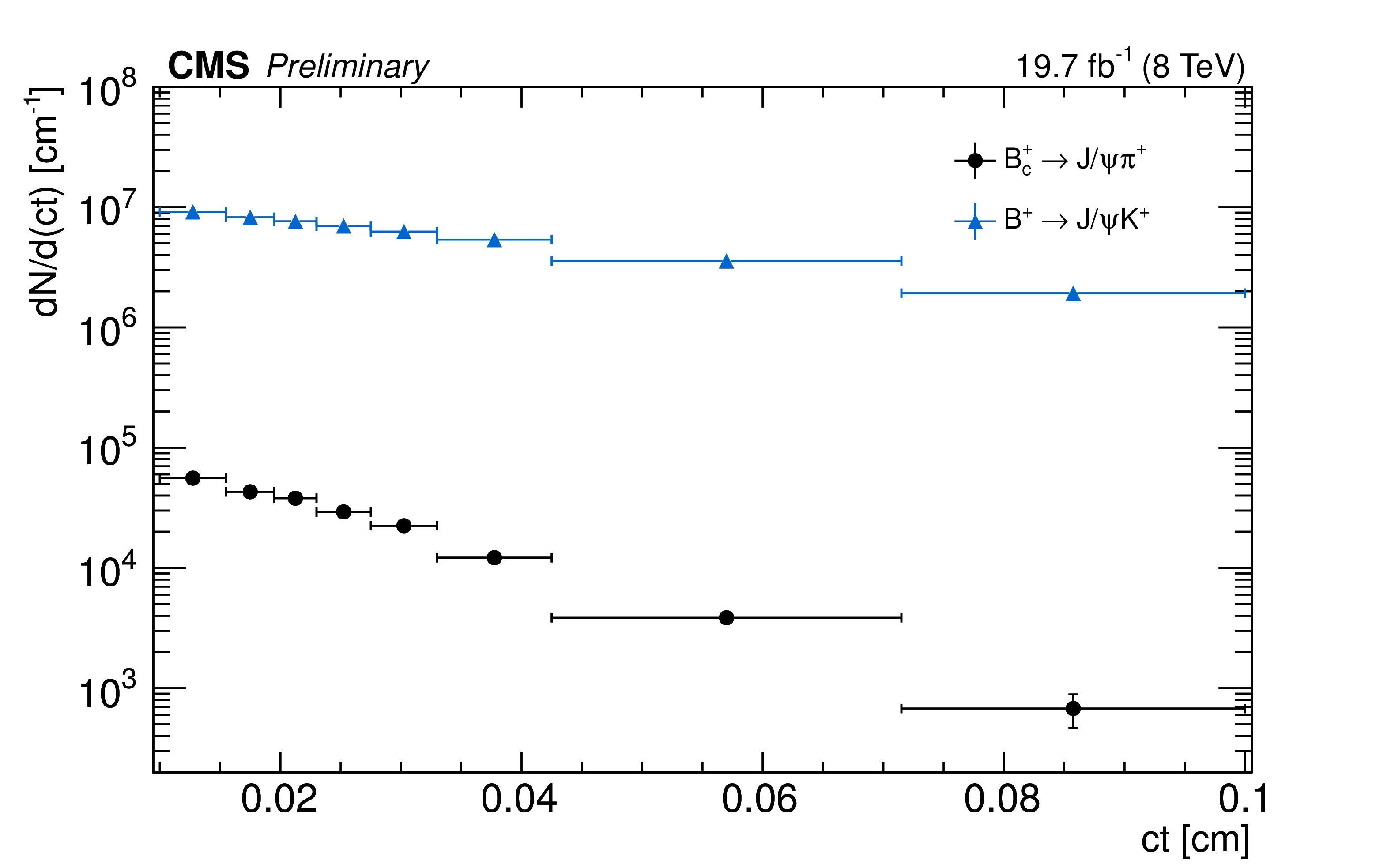
Figure 9-a:
The yield of $\mathrm{B}_{c}^{+} \to \mathrm{J}/\psi\, \pi^{+} $ and $\mathrm{B}^{+} \to \mathrm{J}/\psi\, \mathrm{K}^{+} $ events as a function of $ct$, normalized to the bin width, as determined from fits to the invariant mass distributions. |
png pdf |
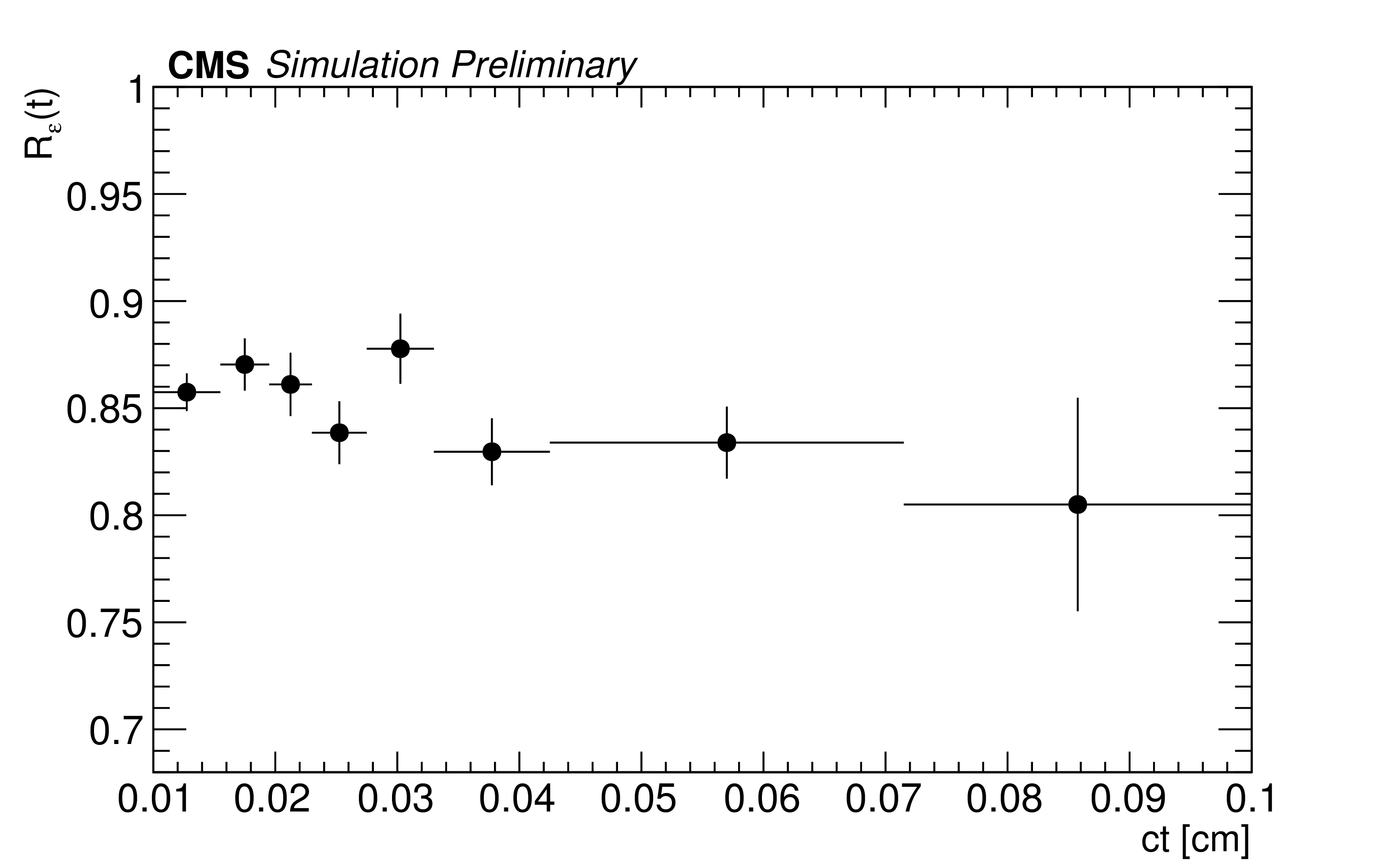
Figure 9-b:
Ratio of the $\mathrm{B}_{c}$ and $\mathrm{B}^{+} $ efficiency distributions as a function of ${ct} $. |
png pdf |
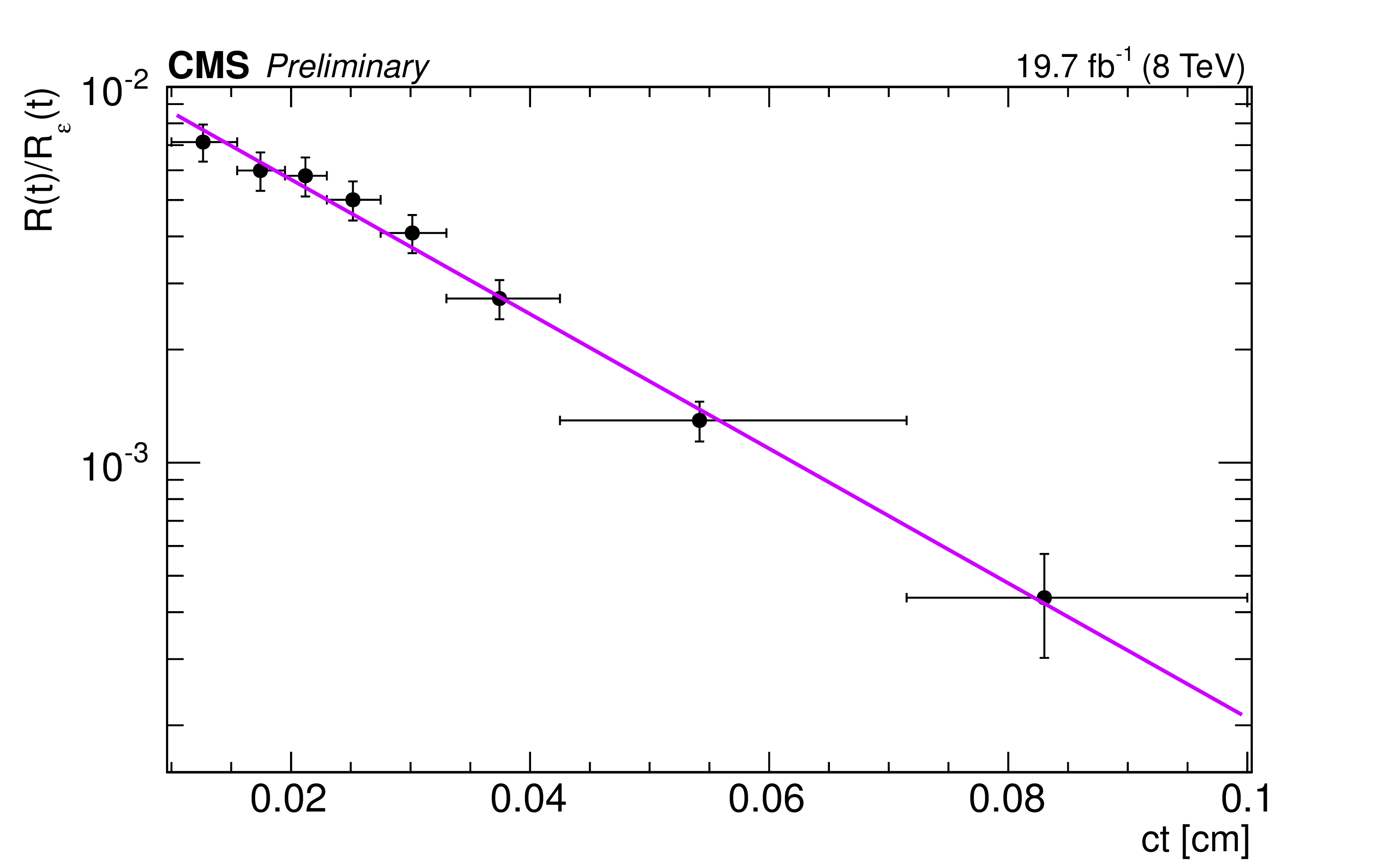
Figure 10:
Ratio of the efficiency-corrected ${ct}$ distributions for $\mathrm{B}_{c}$ and $\mathrm{B}^{+} $ signals. The line shows the result of fitting with an exponential function. |
| Tables | |
png pdf |
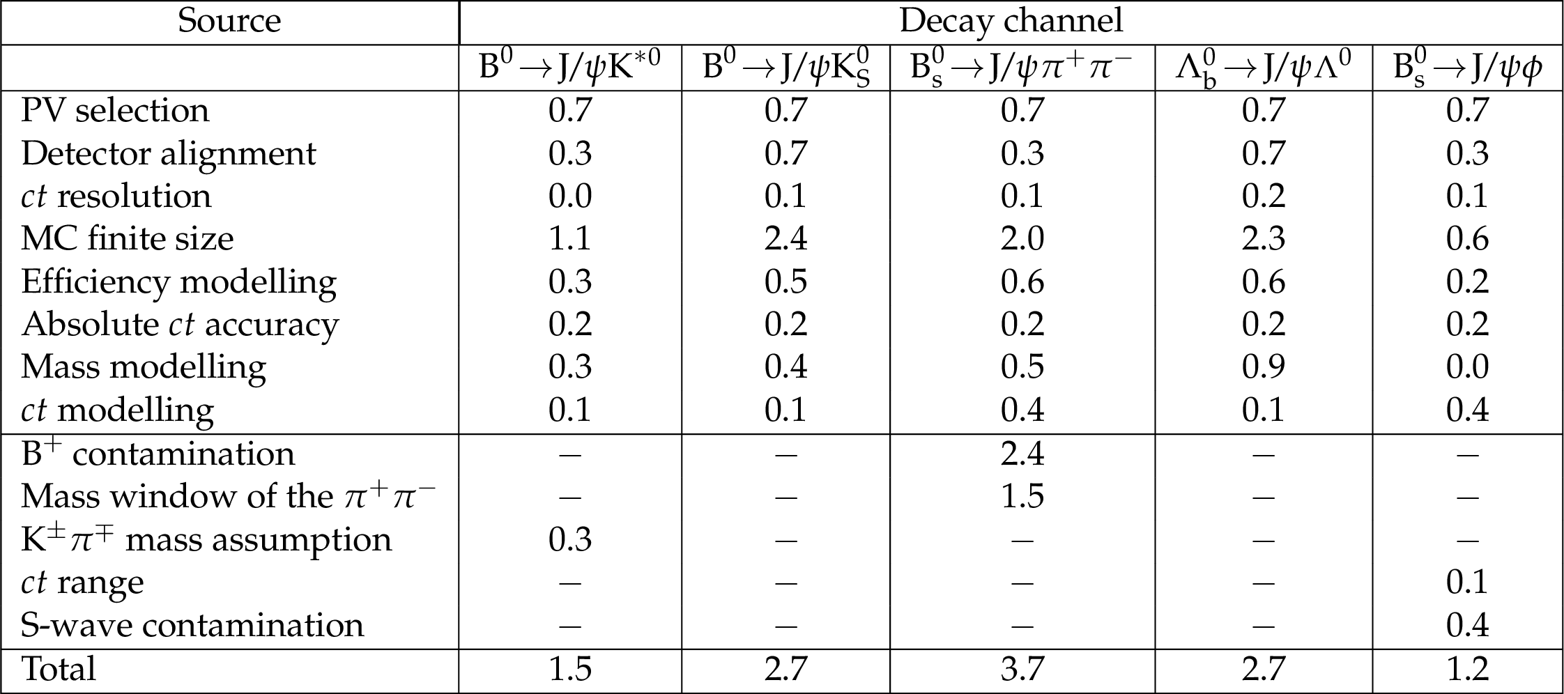
Table 1:
Summary of the systematic uncertainties on the lifetime measurements (in $\mu$m). The total systematic uncertainty is the sum in quadrature of all systematic sources. |
png pdf |
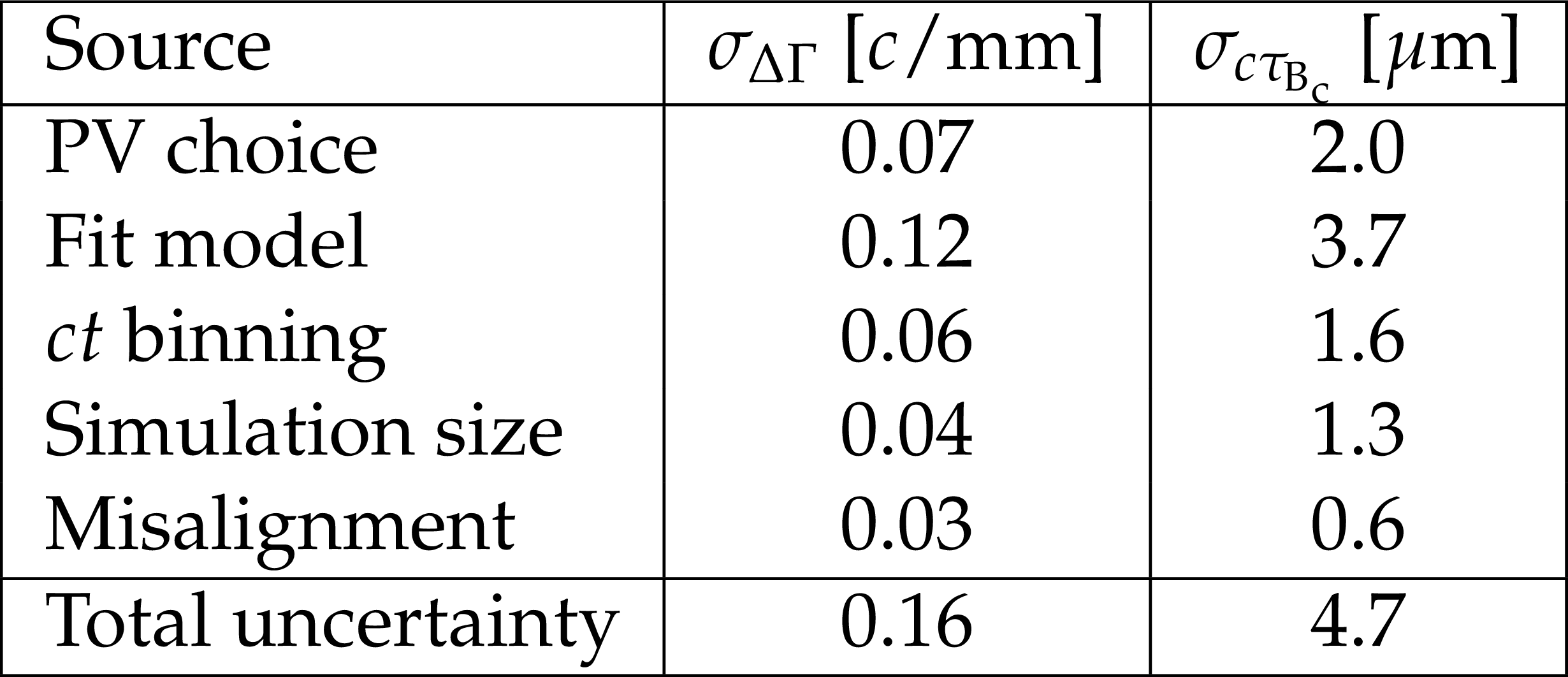
Table 2:
Summary of the systematic uncertainties on the $\Delta \Gamma $ and $\tau _{\mathrm{B}_{c} }$ measurements. |
| Summary |
| The lifetime measurements of the $ \mathrm{B}^0 $, $ \mathrm{B}^0_{s} $, $\mathrm{B}_{c}$, and $\Lambda_\mathrm{b}^0$ hadrons, exploiting the decay channels $\mathrm{B}^0 \to \mathrm{J}/\psi\, \mathrm{K}^{*0}$, $\mathrm{B}^0 \to \mathrm{J}/\psi\, \mathrm{K}_{s}^{0}$, $ \mathrm{B}^0_{s} \to \mathrm{J}/\psi\, \pi^{+} \pi^{-} $, $ \mathrm{B}^0_{s} \to \mathrm{J}/\psi\, \phi$, $\Lambda_\mathrm{b}^0 \to\mathrm{J}/\psi\, \Lambda^{0}$, and $\mathrm{B}^{+} \to \mathrm{J}/\psi\, \pi^{+}$, have been presented, using proton proton collision events collected by the CMS detector at a centre-of-mass energy of 8 TeV, corresponding to an integrated luminosity of 19.7 fb$^{-1}$. All measurements are in agreement with the world average values and some are at the precision of the world average of these parameters. |
| References | ||||
| 1 | CMS Collaboration | Prompt and non-prompt $ J/\psi $ production in pp collisions at $ \sqrt{s} = $ 7 TeV | EPJC 71 (2011) 1575 | CMS-BPH-10-002 1011.4193 |
| 2 | CMS Collaboration | The CMS experiment at the CERN LHC | JINST 3 (2008) S08004 | CMS-00-001 |
| 3 | R. Fleischer and R. Knegjens | Effective lifetimes of $ B_s $ decays and their constraints on the $ B_s^0 $-$ \bar{B}_s^0 $ mixing parameters | EPJC 71 (2011) 1789 | 1109.5115 |
| 4 | Particle Data Group, C. Patrignani et al. | Review of particle physics | CPC 40 (2016) 100001 | |
| 5 | LHCb Collaboration | Analysis of the resonant components in $ \bar{B}_s^0 \to J/\psi \pi^+ \pi^- $ | PRD 86 (2012) 052006 | 1301.5347 |
| 6 | LHCb Collaboration | Measurement of resonant and CP components in $ \bar{B}_s^0 \to J/\psi \pi^+ \pi^- $ | PRD 89 (2014) 092006 | 1402.6248 |
| 7 | CMS Collaboration | Measurement of the CP-violating weak phase $ \phi_s $ and the decay width difference $ \Delta \Gamma_s $ using the $ B _s^0 \to J/\psi\phi (1020)$ decay channel in pp collisions at $ \sqrt{s}= $ 8 TeV | PLB 757 (2016) 97 | CMS-BPH-13-012 1507.07527 |
| 8 | LHCb Collaboration | Measurement of the $ B^+_c $ meson lifetime using $ B^+_c \to J/\psi \mu{+} \nu X $ decays | JHEP 74 (2014) 2839 | 1401.6932 |
| 9 | LHCb Collaboration | Measurement of the lifetime of the $ B^+_c $ meson using the $ B^+_c \to J/\psi \pi^+ $ decay mode | PLB 742 (2015) 29 | 1411.6899 |
| 10 | CDF Collaboration | Measurement of the $ B^+_ c $ meson lifetime using $ B^+_ c \to J/\psi e^+ \nu_e $ | PRL 97 (2006) 012002 | hep-ex/0603027 |
| 11 | CDF Collaboration | Measurement of the $ B^-_ c $ meson lifetime in the decay $ B^-_ c \to J/\psi \pi^- $ | PRD. 87 (2013) 011101 | 1210.2366 |
| 12 | D0 Collaboration | Measurement of the lifetime of the $ B^{\pm}_ c $ meson in the semileptonic decay channel | PRL 102 (2009) 092001 | 0805.2614 |
| 13 | CMS Collaboration | Description and performance of track and primary-vertex reconstruction with the CMS tracker | JINST 9 (2014) P10009 | CMS-TRK-11-001 1405.6569 |
| 14 | T. Sjostrand, S. Mrenna, and P. Z. Skands | PYTHIA 6.4 Physics and Manual | JHEP 05 (2006) 026 | hep-ph/0603175 |
| 15 | C. Chang, C. Driouchi, P. Eerola, and X. Wu | BCVEGPY: an event generator for hadronic production of the $ \mathrm{B_c} $ meson | CPC 159 (2004) 192--224 | hep-ph/0309120 |
| 16 | J. Chang, C Wang and X. Wu | BCVEGPY2.0: An upgraded version of the generator BCVEGPY with the addition of hadroproduction of the P-wave $ \mathrm{B_c} $ states | CPC 174 (2006) 241--251 | hep-ph/0504017 |
| 17 | D. Lange | The EvtGen particle decay simulation package | NIMA 462 (2001) 152 | |
| 18 | P. Golonka and Z. Was | PHOTOS Monte Carlo: a precision tool for QED corrections in Z and W decays | Eur.Phys.J.C 45 (2006) 97 | 0506026 |
| 19 | GEANT4 Collaboration | GEANT4: A Simulation toolkit | NIMA 506 (2003) 250 | |
| 20 | CMS Collaboration | Performance of CMS muon reconstruction in $ pp $ collision events at $ \sqrt{s} = $ 7 TeV | JINST 7 (2012) P10002 | CMS-MUO-10-004 1206.4071 |
| 21 | CMS Collaboration | CMS tracking performance results from early LHC operation | EPJC 70 (2010) 1165 | CMS-TRK-10-001 1007.1988 |
| 22 | LHCb Collaboration | First observation of the decay $ \mathrm{B^+_c }\to \mathrm{J}/\psi \, \mathrm{K}^{+} $ | JHEP 09 (2013) 075 | 1306.6723 |
| 23 | T. Skwarnicki | A staudy of the radiative cascade transitions between the $\Upsilon'$ and the $\Upsilon$ resonances | PhD thesis, Cracow, INP | |
| 24 | M. J. Oreglia | A Study of the Reactions $ \psi' \to \gamma \gamma \psi$ | PhD thesis, Stanford University, 1980 SLAC Report SLAC-R-236, see Appendix D | |
| 25 | FOCUS Collaboration | Study of the Cabibbo-suppressed decay mode $ D^0 \to \pi^-\pi^+ $ and $ D^0 \to K^- K^+ $ | PLB 555 (2003) 167 | |
|
|
Compact Muon Solenoid LHC, CERN |
|

|

|

|

|

|