

Compact Muon Solenoid
LHC, CERN
| CMS-PAS-B2G-17-015 | ||
| Search for a heavy resonance decaying to a top quark and a vector-like top quark in the lepton+jets final state | ||
| CMS Collaboration | ||
| July 2018 | ||
| Abstract: A search is presented for a heavy spin-1 resonance Z' decaying to a top quark and a vector-like top quark T in the lepton+jets final state. The search is performed using a data set of proton-proton collisions at a centre-of-mass energy of 13 TeV corresponding to an integrated luminosity of 35.9 fb$^{-1}$ as recorded by the CMS experiment at the CERN LHC in the year 2016. The analysis is optimised for final states arising from the T decay modes to a top quark and a Higgs or a Z boson ($\mathrm{T} \to \mathrm{Ht},\,\mathrm{Zt}$). The event selection makes use of resolved and boosted top quark decays, as well as boosted decays of H bosons and heavy gauge bosons using jet substructure techniques. No signficant deviation from the standard model background expectation is observed. Model-independent exclusion limits on the product of the cross section and branching fraction are presented for various combinations of the Z' resonance mass and the vector-like T quark mass. In a benchmark model with extra dimensions, masses of the Z' resonance less than 2.4 TeV are excluded. These limits represent the most stringent limits to date for the decay mode $\mathrm{Z}^\prime \to \mathrm{tT} \to \mathrm{tHt}$. | ||
|
Links:
CDS record (PDF) ;
CADI line (restricted) ;
These preliminary results are superseded in this paper, EPJC 79 (2019) 208. The superseded preliminary plots can be found here. |
||
| Figures | |
png pdf |
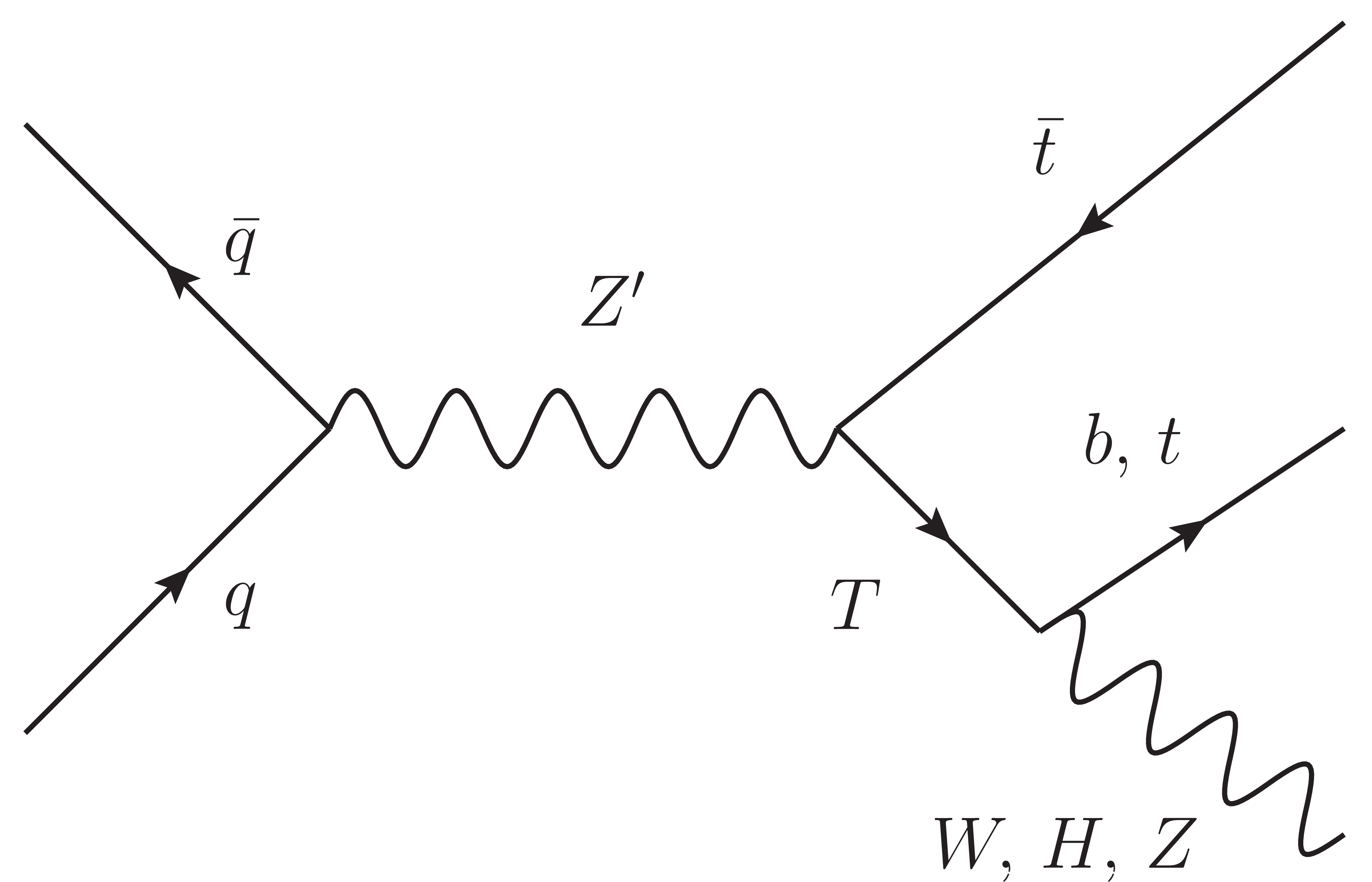
Figure 1:
Feynman diagram for the production of a spin-1 resonance Z' and its decay, along with the possible decays of the vector-like quark T. |
png pdf |
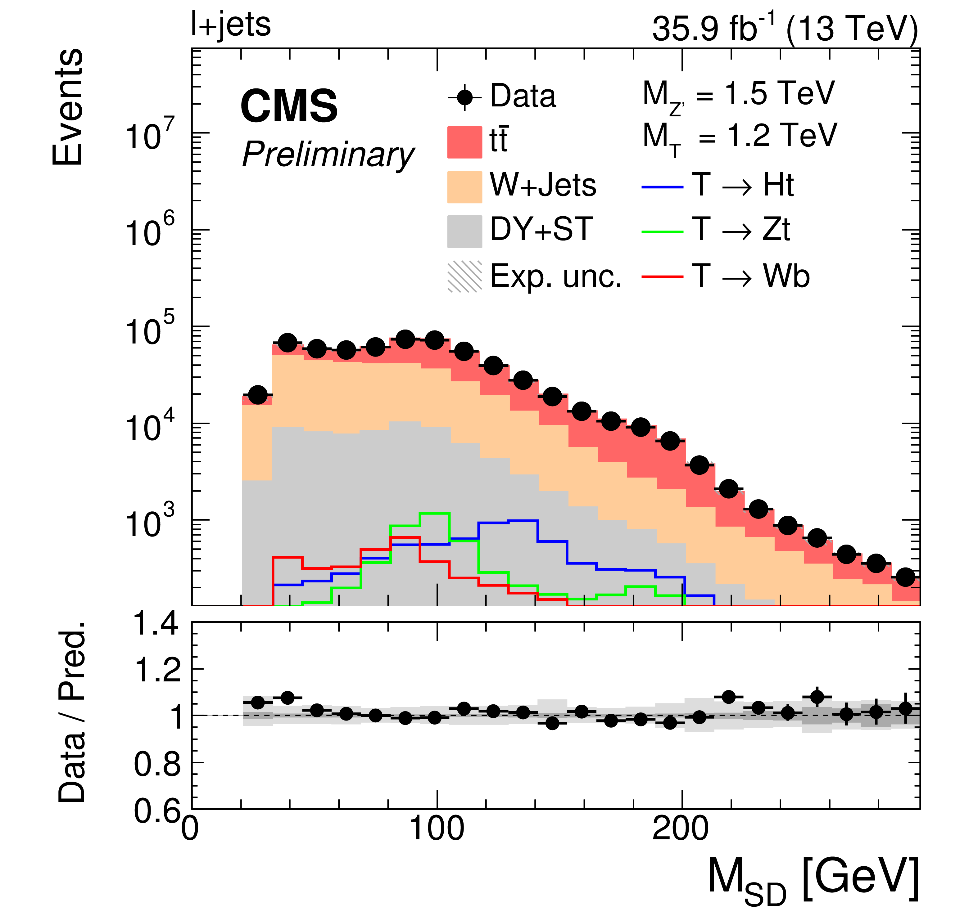
Figure 2:
Distribution of the soft drop mass of jets as reconstructed with the anti-$ {k_{\mathrm {T}}}$ jet algorithm with $R=0.8$ after the selection in data and simulated SM background for the combined lepton+jets channel. The expected signal distribution from various T decay modes is shown for the example mass configuration $ {M_{{{\mathrm {Z}} ^{\prime}}}} = $ 1.5 TeV and $ {M_{{\text {T}}}} = $ 1.2 TeV with a nominal cross section of 1 pb. |
png pdf |
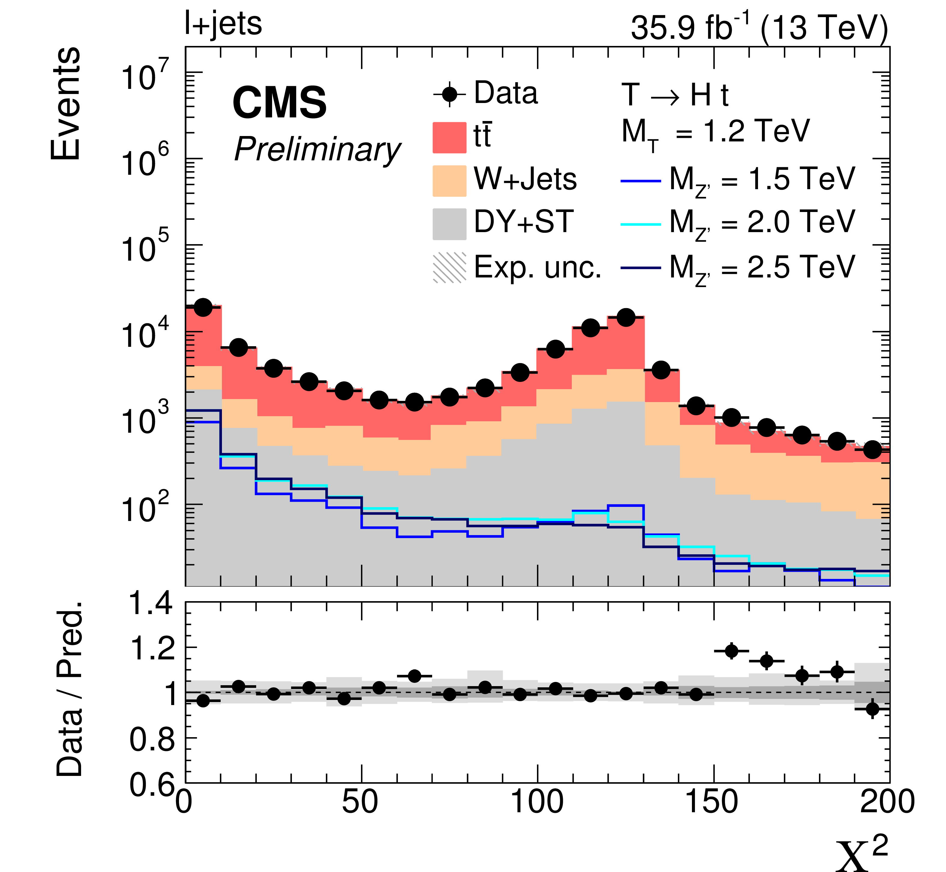
Figure 3:
Distribution of the $ {\chi ^2} $ discriminator for the combination of both top tag and no top tag categories after the $ {{\mathrm {t}\overline {\mathrm {t}}}} $ reconstruction, combining both lepton channels. The expected signal distribution is shown for various $ {M_{{{\mathrm {Z}} ^{\prime}}}} $ masses for a fixed mass $ {M_{{\text {T}}}} = $ 1.2 TeV in the $ {{\text {T}} \to {\mathrm {H}} {\mathrm {t}}}$ decay channel, each with a nominal cross section of 1 pb. |

png pdf |
Figure 4-a:
Distribution of the reconstructed Z' boson mass in the $\mu$+jets channel (top) and e+jets channel (bottom) for the $ {{\mathrm {t}\overline {\mathrm {t}}}} $-enriched control region (left) and for the W+jets-enriched region (right). The expected signal distribution is shown for various $ {M_{{{\mathrm {Z}} ^{\prime}}}} $ masses for a fixed mass $ {M_{{\text {T}}}} = $ 1.2 TeV in the $ {{\text {T}} \to {\mathrm {H}} {\mathrm {t}}}$ decay channel, each with a nominal cross section of 1 pb. |
png pdf |
Figure 4-b:
Distribution of the reconstructed Z' boson mass in the $\mu$+jets channel (top) and e+jets channel (bottom) for the $ {{\mathrm {t}\overline {\mathrm {t}}}} $-enriched control region (left) and for the W+jets-enriched region (right). The expected signal distribution is shown for various $ {M_{{{\mathrm {Z}} ^{\prime}}}} $ masses for a fixed mass $ {M_{{\text {T}}}} = $ 1.2 TeV in the $ {{\text {T}} \to {\mathrm {H}} {\mathrm {t}}}$ decay channel, each with a nominal cross section of 1 pb. |

png pdf |
Figure 4-c:
Distribution of the reconstructed Z' boson mass in the $\mu$+jets channel (top) and e+jets channel (bottom) for the $ {{\mathrm {t}\overline {\mathrm {t}}}} $-enriched control region (left) and for the W+jets-enriched region (right). The expected signal distribution is shown for various $ {M_{{{\mathrm {Z}} ^{\prime}}}} $ masses for a fixed mass $ {M_{{\text {T}}}} = $ 1.2 TeV in the $ {{\text {T}} \to {\mathrm {H}} {\mathrm {t}}}$ decay channel, each with a nominal cross section of 1 pb. |
png pdf |
Figure 4-d:
Distribution of the reconstructed Z' boson mass in the $\mu$+jets channel (top) and e+jets channel (bottom) for the $ {{\mathrm {t}\overline {\mathrm {t}}}} $-enriched control region (left) and for the W+jets-enriched region (right). The expected signal distribution is shown for various $ {M_{{{\mathrm {Z}} ^{\prime}}}} $ masses for a fixed mass $ {M_{{\text {T}}}} = $ 1.2 TeV in the $ {{\text {T}} \to {\mathrm {H}} {\mathrm {t}}}$ decay channel, each with a nominal cross section of 1 pb. |
png pdf |
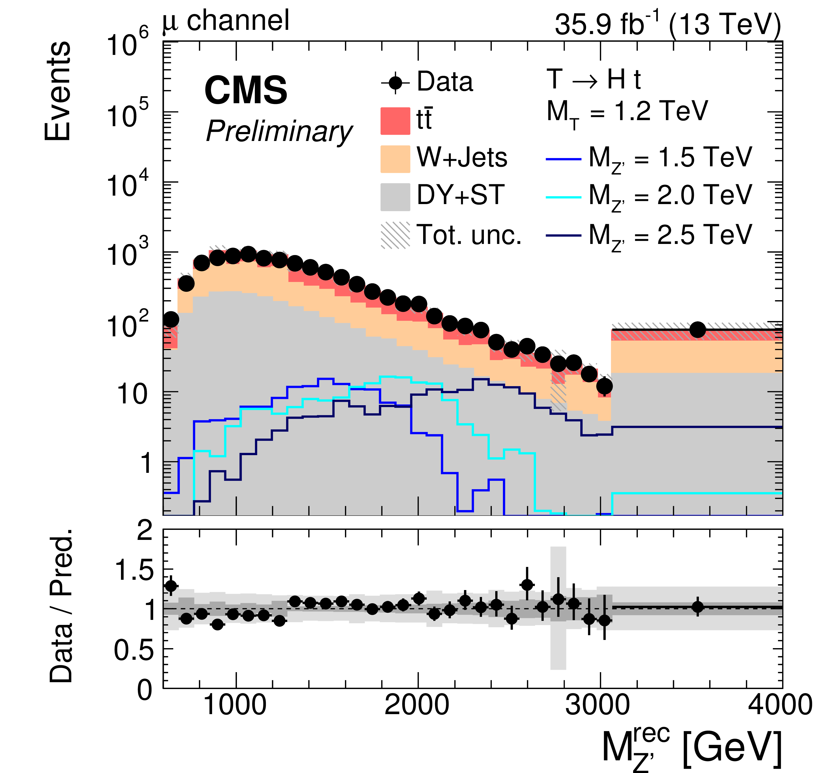
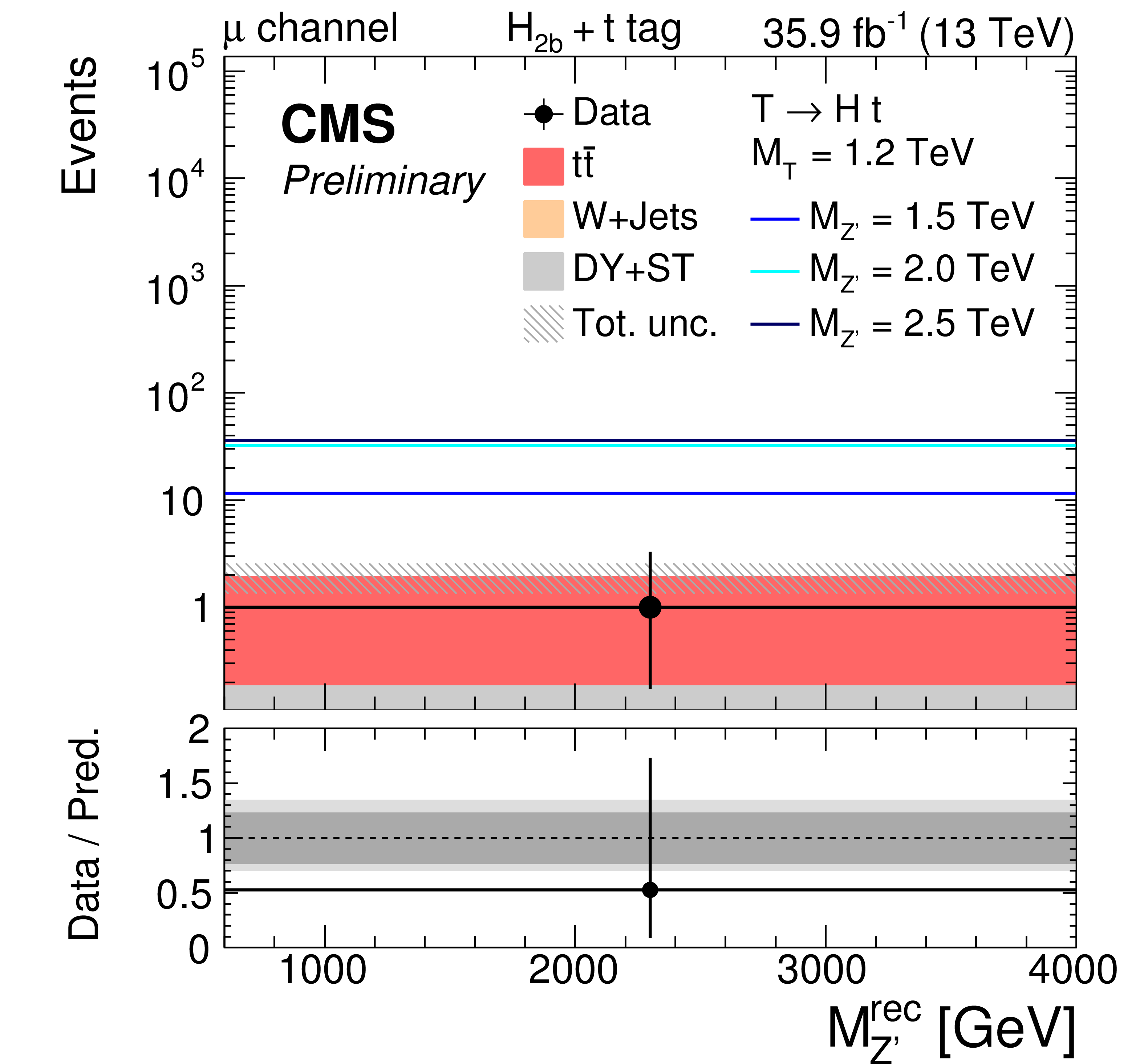
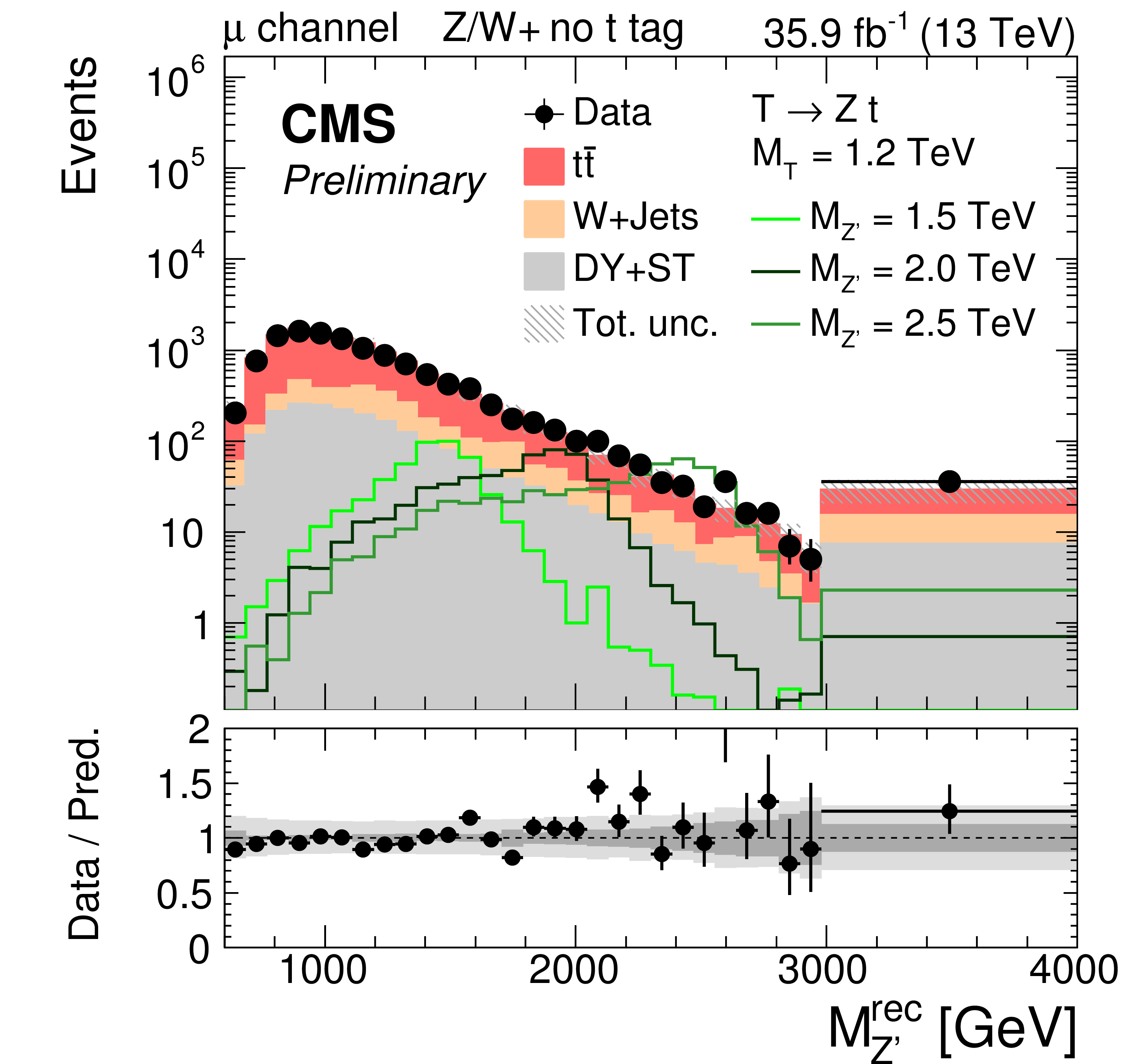
Figure 5-a:
Distribution of the reconstructed resonance mass after the full selection in the $\mu$+jets channel for the data, the expected SM background, and for the signal with different Z' masses for a fixed T mass of 1.2 TeV. In the left (right) column the results in the (no) top tag category are shown. Different rows display the distributions of events accepted by different taggers as well as the signal for the respective T decays: $ {{\mathrm {H}} _{2 {\mathrm {b}}}} $ tagger and $ {{\text {T}} \to {\mathrm {H}} {\mathrm {t}}}$ decay (top), $ {{\mathrm {H}} _{1 {\mathrm {b}}}} $ tagger and $ {{\text {T}} \to {\mathrm {H}} {\mathrm {t}}}$ decay (middle), and $ {\mathrm {Z}} / {\mathrm {W}}$ tagger and $ {{\text {T}} \to {\mathrm {Z}} {\mathrm {t}}}$ decay (bottom). The signal histograms correspond to a nominal cross section of 1 pb. |
png pdf |
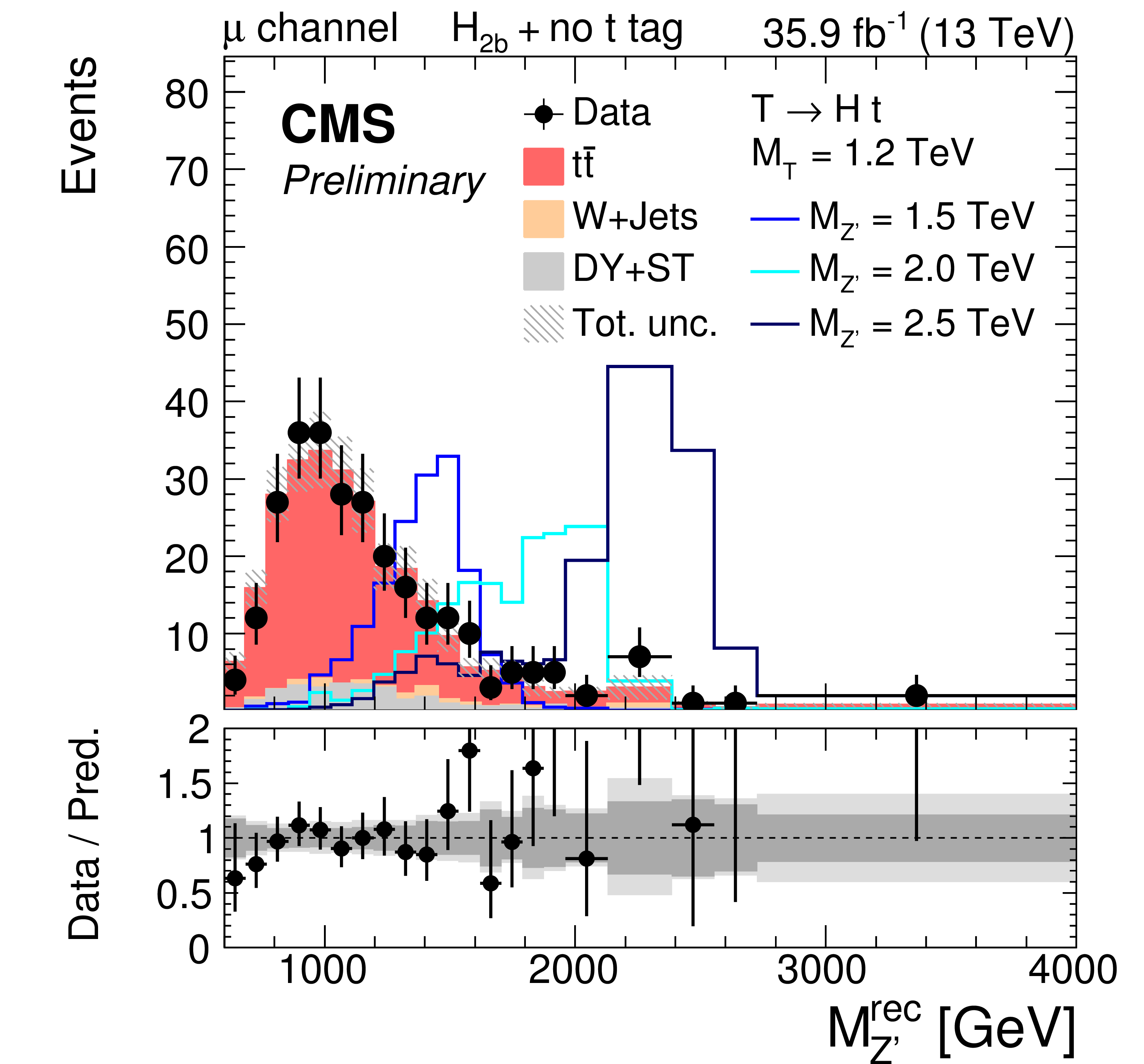
Figure 5-b:
Distribution of the reconstructed resonance mass after the full selection in the $\mu$+jets channel for the data, the expected SM background, and for the signal with different Z' masses for a fixed T mass of 1.2 TeV. In the left (right) column the results in the (no) top tag category are shown. Different rows display the distributions of events accepted by different taggers as well as the signal for the respective T decays: $ {{\mathrm {H}} _{2 {\mathrm {b}}}} $ tagger and $ {{\text {T}} \to {\mathrm {H}} {\mathrm {t}}}$ decay (top), $ {{\mathrm {H}} _{1 {\mathrm {b}}}} $ tagger and $ {{\text {T}} \to {\mathrm {H}} {\mathrm {t}}}$ decay (middle), and $ {\mathrm {Z}} / {\mathrm {W}}$ tagger and $ {{\text {T}} \to {\mathrm {Z}} {\mathrm {t}}}$ decay (bottom). The signal histograms correspond to a nominal cross section of 1 pb. |

png pdf |
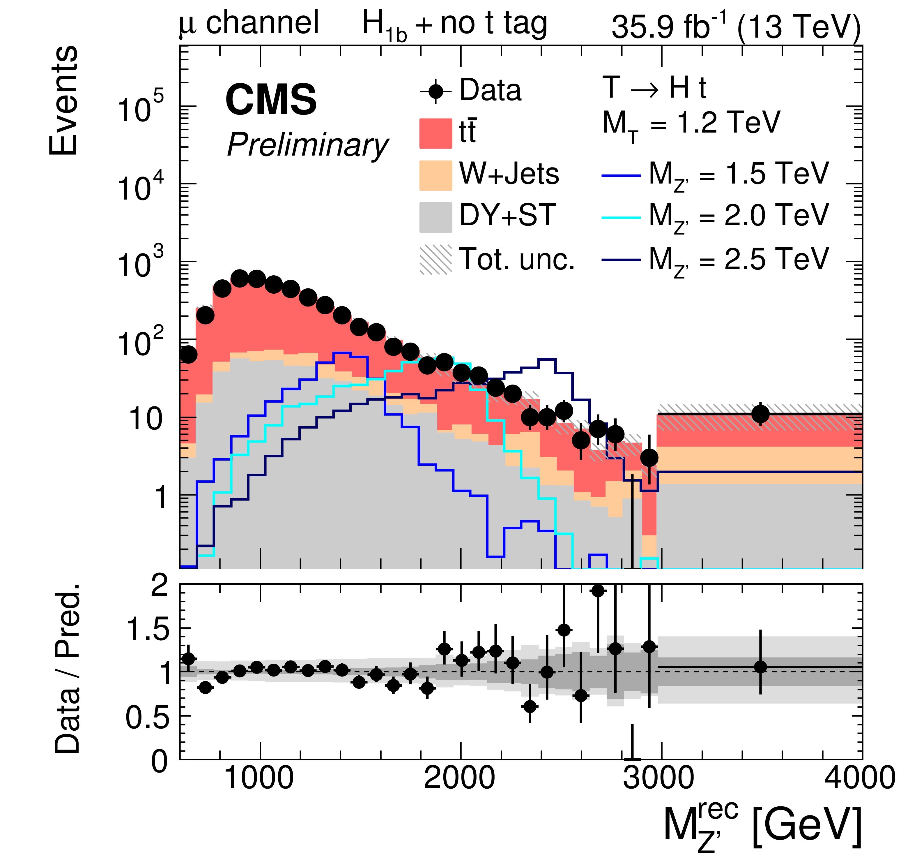
Figure 5-c:
Distribution of the reconstructed resonance mass after the full selection in the $\mu$+jets channel for the data, the expected SM background, and for the signal with different Z' masses for a fixed T mass of 1.2 TeV. In the left (right) column the results in the (no) top tag category are shown. Different rows display the distributions of events accepted by different taggers as well as the signal for the respective T decays: $ {{\mathrm {H}} _{2 {\mathrm {b}}}} $ tagger and $ {{\text {T}} \to {\mathrm {H}} {\mathrm {t}}}$ decay (top), $ {{\mathrm {H}} _{1 {\mathrm {b}}}} $ tagger and $ {{\text {T}} \to {\mathrm {H}} {\mathrm {t}}}$ decay (middle), and $ {\mathrm {Z}} / {\mathrm {W}}$ tagger and $ {{\text {T}} \to {\mathrm {Z}} {\mathrm {t}}}$ decay (bottom). The signal histograms correspond to a nominal cross section of 1 pb. |
png pdf |
Figure 5-d:
Distribution of the reconstructed resonance mass after the full selection in the $\mu$+jets channel for the data, the expected SM background, and for the signal with different Z' masses for a fixed T mass of 1.2 TeV. In the left (right) column the results in the (no) top tag category are shown. Different rows display the distributions of events accepted by different taggers as well as the signal for the respective T decays: $ {{\mathrm {H}} _{2 {\mathrm {b}}}} $ tagger and $ {{\text {T}} \to {\mathrm {H}} {\mathrm {t}}}$ decay (top), $ {{\mathrm {H}} _{1 {\mathrm {b}}}} $ tagger and $ {{\text {T}} \to {\mathrm {H}} {\mathrm {t}}}$ decay (middle), and $ {\mathrm {Z}} / {\mathrm {W}}$ tagger and $ {{\text {T}} \to {\mathrm {Z}} {\mathrm {t}}}$ decay (bottom). The signal histograms correspond to a nominal cross section of 1 pb. |

png pdf |
Figure 5-e:
Distribution of the reconstructed resonance mass after the full selection in the $\mu$+jets channel for the data, the expected SM background, and for the signal with different Z' masses for a fixed T mass of 1.2 TeV. In the left (right) column the results in the (no) top tag category are shown. Different rows display the distributions of events accepted by different taggers as well as the signal for the respective T decays: $ {{\mathrm {H}} _{2 {\mathrm {b}}}} $ tagger and $ {{\text {T}} \to {\mathrm {H}} {\mathrm {t}}}$ decay (top), $ {{\mathrm {H}} _{1 {\mathrm {b}}}} $ tagger and $ {{\text {T}} \to {\mathrm {H}} {\mathrm {t}}}$ decay (middle), and $ {\mathrm {Z}} / {\mathrm {W}}$ tagger and $ {{\text {T}} \to {\mathrm {Z}} {\mathrm {t}}}$ decay (bottom). The signal histograms correspond to a nominal cross section of 1 pb. |
png pdf |
Figure 5-f:
Distribution of the reconstructed resonance mass after the full selection in the $\mu$+jets channel for the data, the expected SM background, and for the signal with different Z' masses for a fixed T mass of 1.2 TeV. In the left (right) column the results in the (no) top tag category are shown. Different rows display the distributions of events accepted by different taggers as well as the signal for the respective T decays: $ {{\mathrm {H}} _{2 {\mathrm {b}}}} $ tagger and $ {{\text {T}} \to {\mathrm {H}} {\mathrm {t}}}$ decay (top), $ {{\mathrm {H}} _{1 {\mathrm {b}}}} $ tagger and $ {{\text {T}} \to {\mathrm {H}} {\mathrm {t}}}$ decay (middle), and $ {\mathrm {Z}} / {\mathrm {W}}$ tagger and $ {{\text {T}} \to {\mathrm {Z}} {\mathrm {t}}}$ decay (bottom). The signal histograms correspond to a nominal cross section of 1 pb. |

png pdf |
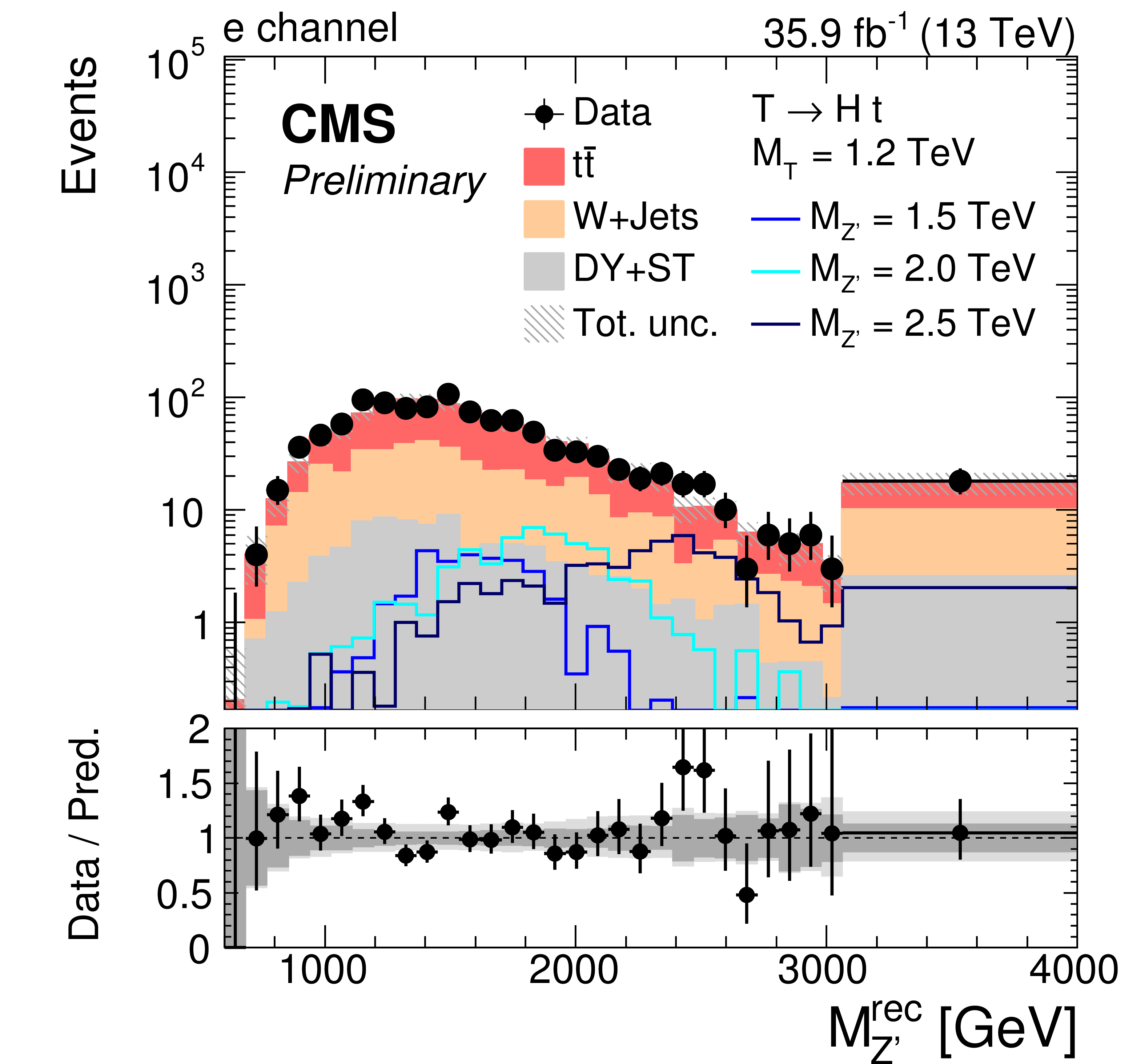
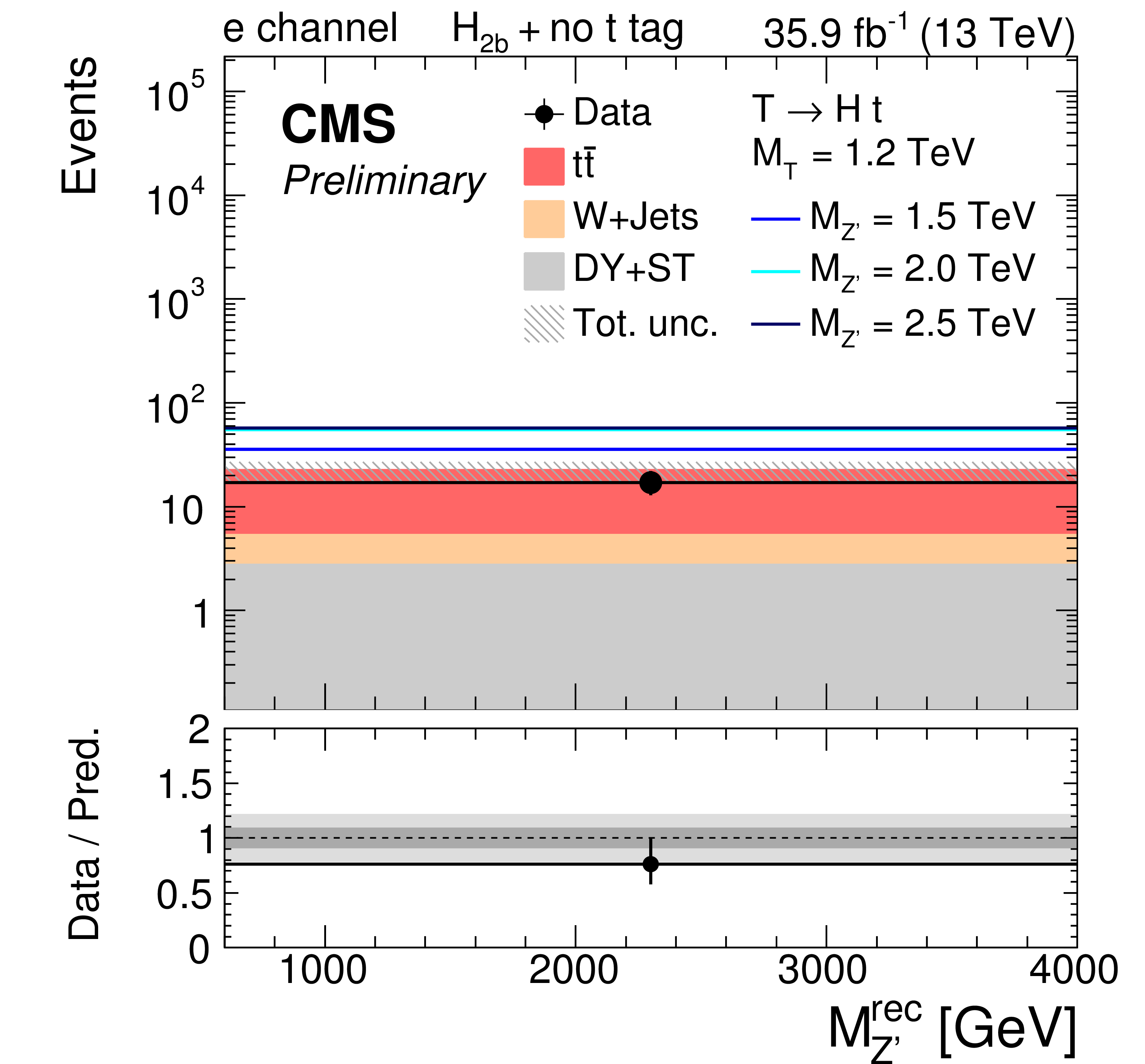
Figure 6-a:
Distribution of the reconstructed resonance mass after the full selection in the e+jets channel for the data, the expected SM background, and for the signal with different Z' masses for a fixed T mass of 1.2 TeV. In the left (right) column the results in the (no) top tag category are shown. Different rows display the distributions of events accepted by different taggers as well as the signal for the respective T decays: $ {{\mathrm {H}} _{2 {\mathrm {b}}}} $ tagger and $ {{\text {T}} \to {\mathrm {H}} {\mathrm {t}}}$ decay (top), $ {{\mathrm {H}} _{1 {\mathrm {b}}}} $ tagger and $ {{\text {T}} \to {\mathrm {H}} {\mathrm {t}}}$ decay (middle), and $ {\mathrm {Z}} / {\mathrm {W}}$ tagger and $ {{\text {T}} \to {\mathrm {Z}} {\mathrm {t}}}$ decay (bottom). The signal histograms correspond to a nominal cross section of 1 pb. |
png pdf |
Figure 6-b:
Distribution of the reconstructed resonance mass after the full selection in the e+jets channel for the data, the expected SM background, and for the signal with different Z' masses for a fixed T mass of 1.2 TeV. In the left (right) column the results in the (no) top tag category are shown. Different rows display the distributions of events accepted by different taggers as well as the signal for the respective T decays: $ {{\mathrm {H}} _{2 {\mathrm {b}}}} $ tagger and $ {{\text {T}} \to {\mathrm {H}} {\mathrm {t}}}$ decay (top), $ {{\mathrm {H}} _{1 {\mathrm {b}}}} $ tagger and $ {{\text {T}} \to {\mathrm {H}} {\mathrm {t}}}$ decay (middle), and $ {\mathrm {Z}} / {\mathrm {W}}$ tagger and $ {{\text {T}} \to {\mathrm {Z}} {\mathrm {t}}}$ decay (bottom). The signal histograms correspond to a nominal cross section of 1 pb. |

png pdf |
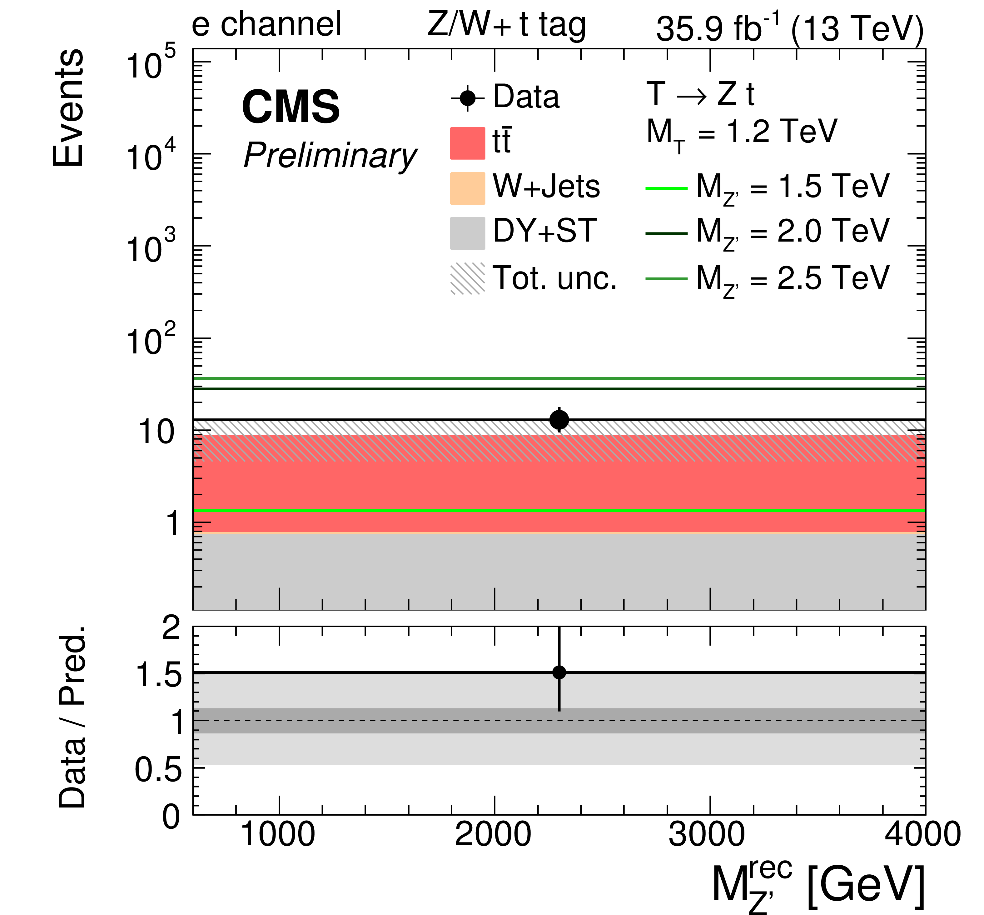
Figure 6-c:
Distribution of the reconstructed resonance mass after the full selection in the e+jets channel for the data, the expected SM background, and for the signal with different Z' masses for a fixed T mass of 1.2 TeV. In the left (right) column the results in the (no) top tag category are shown. Different rows display the distributions of events accepted by different taggers as well as the signal for the respective T decays: $ {{\mathrm {H}} _{2 {\mathrm {b}}}} $ tagger and $ {{\text {T}} \to {\mathrm {H}} {\mathrm {t}}}$ decay (top), $ {{\mathrm {H}} _{1 {\mathrm {b}}}} $ tagger and $ {{\text {T}} \to {\mathrm {H}} {\mathrm {t}}}$ decay (middle), and $ {\mathrm {Z}} / {\mathrm {W}}$ tagger and $ {{\text {T}} \to {\mathrm {Z}} {\mathrm {t}}}$ decay (bottom). The signal histograms correspond to a nominal cross section of 1 pb. |

png pdf |
Figure 6-d:
Distribution of the reconstructed resonance mass after the full selection in the e+jets channel for the data, the expected SM background, and for the signal with different Z' masses for a fixed T mass of 1.2 TeV. In the left (right) column the results in the (no) top tag category are shown. Different rows display the distributions of events accepted by different taggers as well as the signal for the respective T decays: $ {{\mathrm {H}} _{2 {\mathrm {b}}}} $ tagger and $ {{\text {T}} \to {\mathrm {H}} {\mathrm {t}}}$ decay (top), $ {{\mathrm {H}} _{1 {\mathrm {b}}}} $ tagger and $ {{\text {T}} \to {\mathrm {H}} {\mathrm {t}}}$ decay (middle), and $ {\mathrm {Z}} / {\mathrm {W}}$ tagger and $ {{\text {T}} \to {\mathrm {Z}} {\mathrm {t}}}$ decay (bottom). The signal histograms correspond to a nominal cross section of 1 pb. |
png pdf |
Figure 6-e:
Distribution of the reconstructed resonance mass after the full selection in the e+jets channel for the data, the expected SM background, and for the signal with different Z' masses for a fixed T mass of 1.2 TeV. In the left (right) column the results in the (no) top tag category are shown. Different rows display the distributions of events accepted by different taggers as well as the signal for the respective T decays: $ {{\mathrm {H}} _{2 {\mathrm {b}}}} $ tagger and $ {{\text {T}} \to {\mathrm {H}} {\mathrm {t}}}$ decay (top), $ {{\mathrm {H}} _{1 {\mathrm {b}}}} $ tagger and $ {{\text {T}} \to {\mathrm {H}} {\mathrm {t}}}$ decay (middle), and $ {\mathrm {Z}} / {\mathrm {W}}$ tagger and $ {{\text {T}} \to {\mathrm {Z}} {\mathrm {t}}}$ decay (bottom). The signal histograms correspond to a nominal cross section of 1 pb. |

png pdf |
Figure 6-f:
Distribution of the reconstructed resonance mass after the full selection in the e+jets channel for the data, the expected SM background, and for the signal with different Z' masses for a fixed T mass of 1.2 TeV. In the left (right) column the results in the (no) top tag category are shown. Different rows display the distributions of events accepted by different taggers as well as the signal for the respective T decays: $ {{\mathrm {H}} _{2 {\mathrm {b}}}} $ tagger and $ {{\text {T}} \to {\mathrm {H}} {\mathrm {t}}}$ decay (top), $ {{\mathrm {H}} _{1 {\mathrm {b}}}} $ tagger and $ {{\text {T}} \to {\mathrm {H}} {\mathrm {t}}}$ decay (middle), and $ {\mathrm {Z}} / {\mathrm {W}}$ tagger and $ {{\text {T}} \to {\mathrm {Z}} {\mathrm {t}}}$ decay (bottom). The signal histograms correspond to a nominal cross section of 1 pb. |

png pdf |
Figure 7-a:
Exclusion limits at 95% CL on the production cross section for various ($ {M_{{{\mathrm {Z}} ^{\prime}}}}, {M_{{\text {T}}}} $) combinations assuming a T branching fraction of 100% in the decay $ {{\text {T}} \to {\mathrm {H}} {\mathrm {t}}}$ (upper left), $ {{\text {T}} \to {\mathrm {Z}} {\mathrm {t}}}$ (upper right), and $ {{\text {T}} \to {\mathrm {W}} {\mathrm {b}}}$ (lower). |

png pdf |
Figure 7-b:
Exclusion limits at 95% CL on the production cross section for various ($ {M_{{{\mathrm {Z}} ^{\prime}}}}, {M_{{\text {T}}}} $) combinations assuming a T branching fraction of 100% in the decay $ {{\text {T}} \to {\mathrm {H}} {\mathrm {t}}}$ (upper left), $ {{\text {T}} \to {\mathrm {Z}} {\mathrm {t}}}$ (upper right), and $ {{\text {T}} \to {\mathrm {W}} {\mathrm {b}}}$ (lower). |
png pdf |
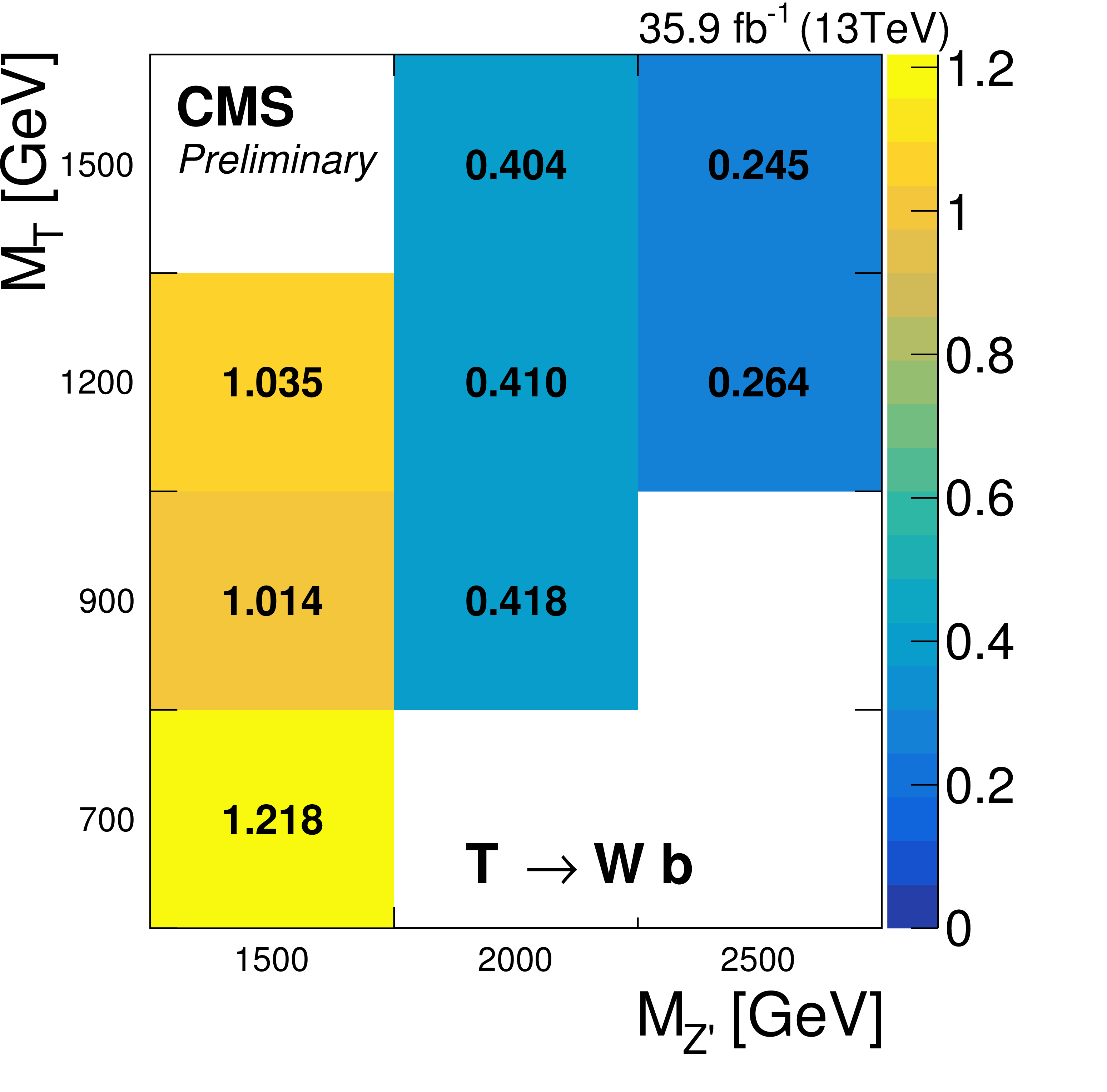
Figure 7-c:
Exclusion limits at 95% CL on the production cross section for various ($ {M_{{{\mathrm {Z}} ^{\prime}}}}, {M_{{\text {T}}}} $) combinations assuming a T branching fraction of 100% in the decay $ {{\text {T}} \to {\mathrm {H}} {\mathrm {t}}}$ (upper left), $ {{\text {T}} \to {\mathrm {Z}} {\mathrm {t}}}$ (upper right), and $ {{\text {T}} \to {\mathrm {W}} {\mathrm {b}}}$ (lower). |
png pdf |
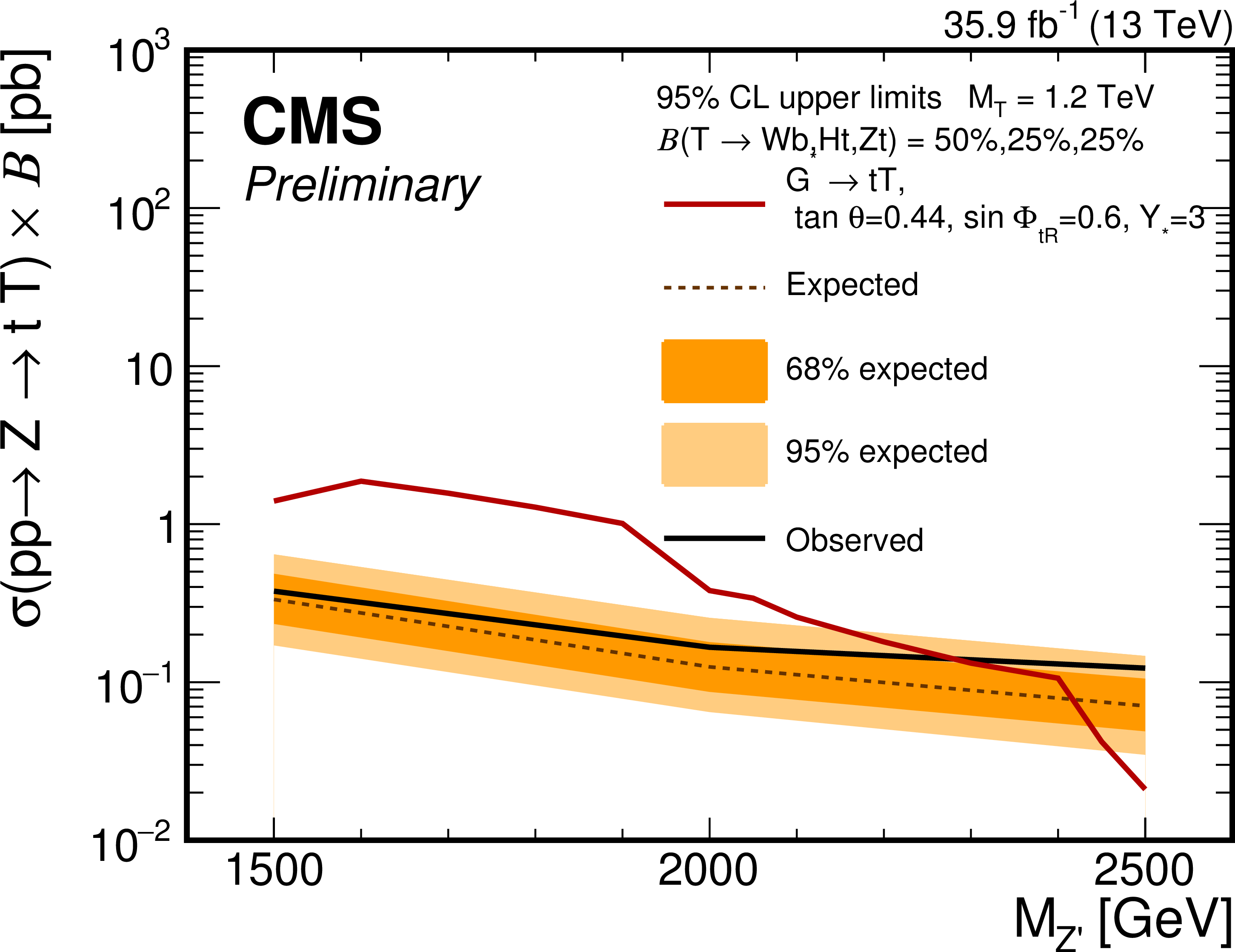
Figure 8-a:
Exclusion limits at 95% CL on the product of the cross section and branching fraction for an example T mass of 1.2 TeV as a function of the resonance mass for two different decay scenarios. Observed and expected limits are compared to the prediction of two different theory benchmark models, the $G^*$ model (left) and the $\rho ^0$ model (right). |
png pdf |
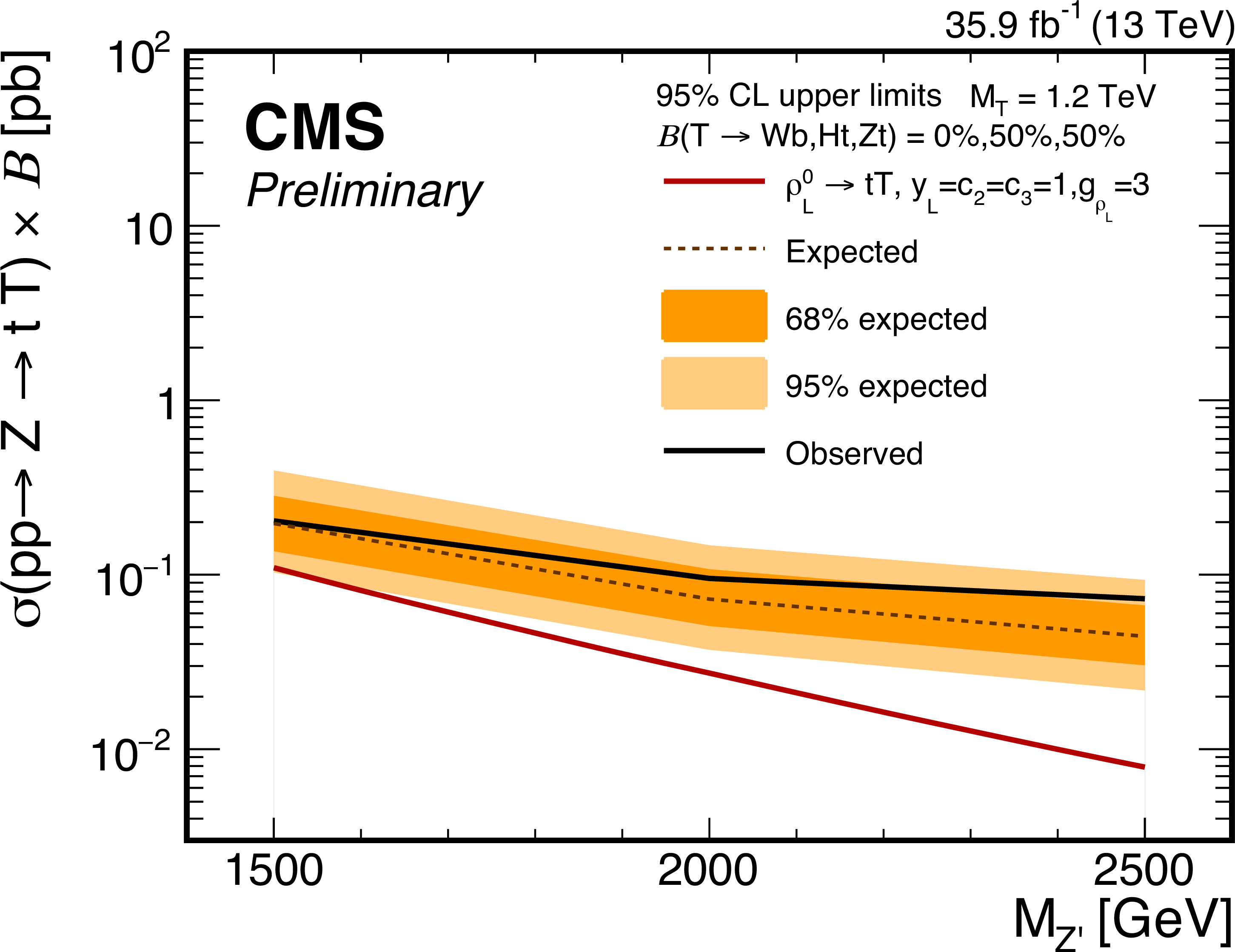
Figure 8-b:
Exclusion limits at 95% CL on the product of the cross section and branching fraction for an example T mass of 1.2 TeV as a function of the resonance mass for two different decay scenarios. Observed and expected limits are compared to the prediction of two different theory benchmark models, the $G^*$ model (left) and the $\rho ^0$ model (right). |
png pdf |
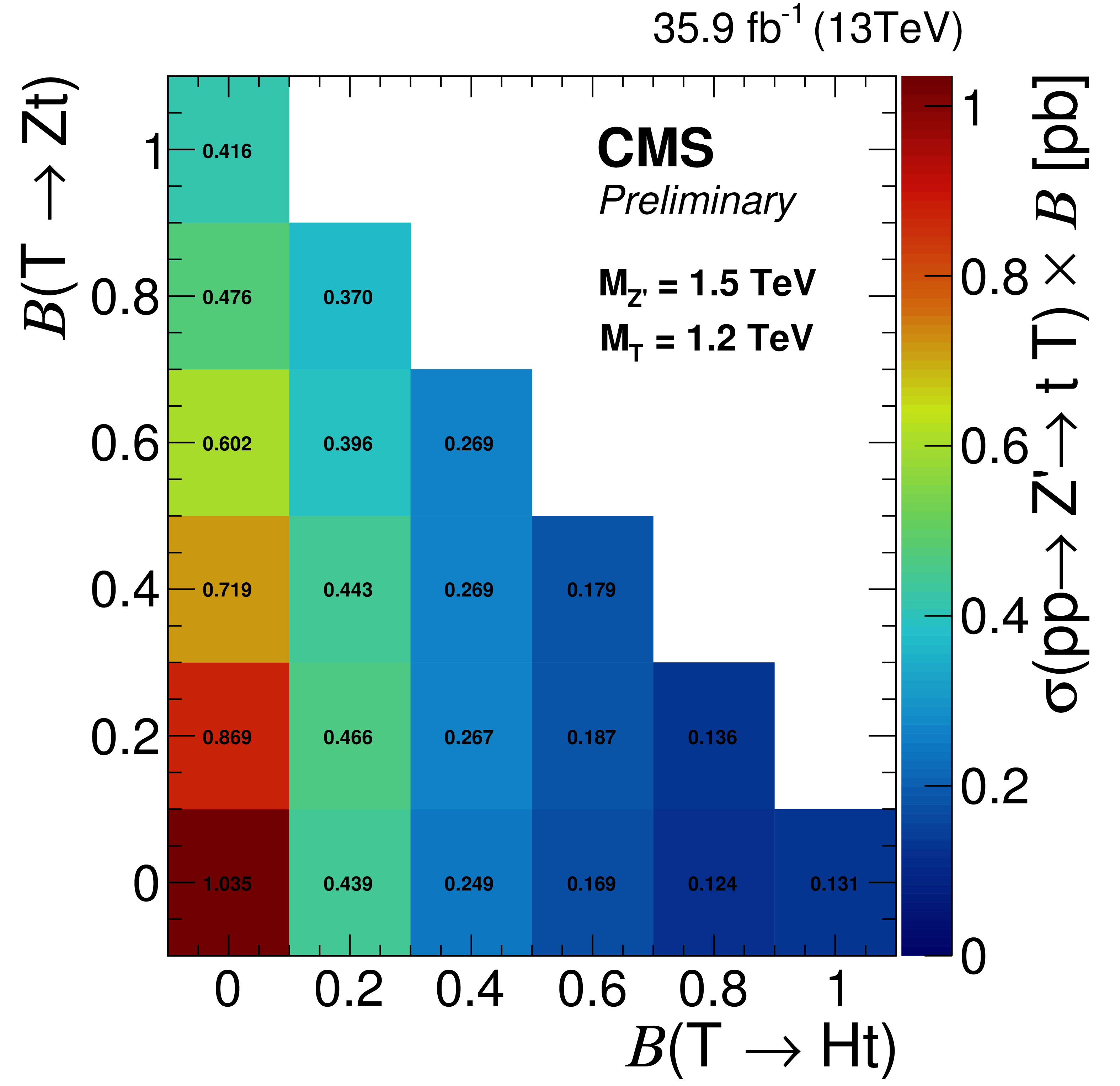
Figure 9:
Exclusion limits at 95% CL on the product of the cross section and branching fraction for an example mass configuration of $ {M_{{{\mathrm {Z}} ^{\prime}}}} = $ 1.5 TeV and $ {M_{{\text {T}}}} = $ 1.2 TeV as a function of the branching fractions, $\mathcal {B}({{\text {T}} \to {\mathrm {H}} {\mathrm {t}}})$ and $\mathcal {B}({{\text {T}} \to {\mathrm {Z}} {\mathrm {t}}})$. |
| Summary |
| A search for a heavy spin-1 resonance Z' decaying to a SM top quark and a vector-like quark T was presented. |
| References | ||||
| 1 | D. Greco and D. Liu | Hunting composite vector resonances at the LHC: naturalness facing data | JHEP 12 (2014) 126 | 1410.2883 |
| 2 | C. Bini, R. Contino, and N. Vignaroli | Heavy-light decay topologies as a new strategy to discover a heavy gluon | JHEP 01 (2012) 157 | 1110.6058 |
| 3 | CMS Collaboration | Search for $ \mathrm{t}\overline{\mathrm{t}} $ resonances in highly boosted lepton+jets and fully hadronic final states in proton-proton collisions at $ \sqrt{s}= $ 13 TeV | JHEP 07 (2017) 001 | CMS-B2G-16-015 1704.03366 |
| 4 | ATLAS Collaboration | A search for $ t\overline{t} $ resonances using lepton-plus-jets events in proton-proton collisions at $ \sqrt{s}= $ 8 TeV with the ATLAS detector | JHEP 08 (2015) 148 | 1505.07018 |
| 5 | A. De Simone, O. Matsedonskyi, R. Rattazzi, and A. Wulzer | A First Top Partner Hunter's Guide | JHEP 04 (2013) 004 | 1211.5663 |
| 6 | R. Contino, D. Marzocca, D. Pappadopulo, and R. Rattazzi | On the effect of resonances in composite Higgs phenomenology | JHEP 10 (2011) 081 | 1109.1570 |
| 7 | L. Randall and R. Sundrum | A large mass hierarchy from a small extra dimension | PRL 83 (1999) 3370 | hep-ph/9905221 |
| 8 | H. Davoudiasl, J. L. Hewett, and T. G. Rizzo | Bulk gauge fields in the Randall-Sundrum model | PLB 473 (2000) 43 | hep-ph/9911262 |
| 9 | J. A. Aguilar-Saavedra, R. Benbrik, S. Heinemeyer, and M. P\'erez-Victoria | Handbook of vectorlike quarks: Mixing and single production | PRD 88 (2013), no. 9, 094010 | 1306.0572 |
| 10 | CMS Collaboration | Search for a heavy resonance decaying to a top quark and a vector-like top quark at $ \sqrt{s}= $ 13 TeV | JHEP 09 (2017) 053 | CMS-B2G-16-013 1703.06352 |
| 11 | CMS Collaboration | Search for single production of a vector-like T quark decaying to a Z boson and a top quark in proton-proton collisions at $ \sqrt s = $ 13 TeV | PLB 781 (2018) 574 | CMS-B2G-17-007 1708.01062 |
| 12 | CMS Collaboration | CMS Luminosity Measurements for the 2016 Data Taking Period | CMS-PAS-LUM-17-001 | CMS-PAS-LUM-17-001 |
| 13 | CMS Collaboration | Jet algorithms performance in 13 TeV data | CMS-PAS-JME-16-003 | CMS-PAS-JME-16-003 |
| 14 | CMS Collaboration | The CMS experiment at the CERN LHC | JINST 3 (2008) S08004 | CMS-00-001 |
| 15 | CMS Collaboration | Particle-flow reconstruction and global event description with the CMS detector | JINST 12 (2017) P10003 | CMS-PRF-14-001 1706.04965 |
| 16 | M. Cacciari, G. P. Salam, and G. Soyez | The anti-$ k_t $ jet clustering algorithm | JHEP 04 (2008) 063 | 0802.1189 |
| 17 | M. Cacciari, G. P. Salam, and G. Soyez | FastJet User Manual | EPJC 72 (2012) 1896 | 1111.6097 |
| 18 | CMS Collaboration | Performance of CMS muon reconstruction in pp collision events at $ \sqrt{s}= $ 7 TeV | JINST 7 (2012) P10002 | CMS-MUO-10-004 1206.4071 |
| 19 | CMS Collaboration | Performance of electron reconstruction and selection with the CMS detector in proton-proton collisions at $ \sqrt{s}= $ 8 TeV | JINST 10 (2015) P06005 | CMS-EGM-13-001 1502.02701 |
| 20 | CMS Collaboration | Jet energy scale and resolution in the CMS experiment in pp collisions at 8 TeV | JINST 12 (2017) P02014 | CMS-JME-13-004 1607.03663 |
| 21 | CMS Collaboration | Identification of heavy-flavour jets with the CMS detector in pp collisions at 13 TeV | JINST 13 (2018) P05011 | CMS-BTV-16-002 1712.07158 |
| 22 | J. Thaler and K. Van Tilburg | Identifying boosted objects with N-subjettiness | JHEP 03 (2011) 015 | 1011.2268 |
| 23 | M. Dasgupta, A. Fregoso, S. Marzani, and G. P. Salam | Towards an understanding of jet substructure | JHEP 09 (2013) 029 | 1307.0007 |
| 24 | J. M. Butterworth, A. R. Davison, M. Rubin, and G. P. Salam | Jet substructure as a new Higgs search channel at the LHC | PRL 100 (2008) 242001 | 0802.2470 |
| 25 | A. J. Larkoski, S. Marzani, G. Soyez, and J. Thaler | Soft Drop | JHEP 05 (2014) 146 | 1402.2657 |
| 26 | J. Alwall et al. | The automated computation of tree-level and next-to-leading order differential cross sections, and their matching to parton shower simulations | JHEP 07 (2014) 079 | 1405.0301 |
| 27 | T. Sjostrand et al. | An Introduction to PYTHIA 8.2 | CPC 191 (2015) 159 | 1410.3012 |
| 28 | R. Frederix and S. Frixione | Merging meets matching in MC@NLO | JHEP 12 (2012) 061 | 1209.6215 |
| 29 | P. Skands, S. Carrazza, and J. Rojo | Tuning PYTHIA 8.1: the Monash 2013 tune | EPJC 74 (2014) 3024 | 1404.5630 |
| 30 | CMS Collaboration | Event generator tunes obtained from underlying event and multiparton scattering measurements | EPJC 76 (2016) 155 | CMS-GEN-14-001 1512.00815 |
| 31 | P. Nason | A new method for combining NLO QCD with shower Monte Carlo algorithms | JHEP 11 (2004) 040 | hep-ph/0409146 |
| 32 | S. Frixione, P. Nason, and C. Oleari | Matching NLO QCD computations with parton shower simulations: the POWHEG method | JHEP 11 (2007) 070 | 0709.2092 |
| 33 | S. Alioli, P. Nason, C. Oleari, and E. Re | A general framework for implementing NLO calculations in shower Monte Carlo programs: the POWHEG BOX | JHEP 06 (2010) 043 | 1002.2581 |
| 34 | S. Alioli, S.-O. Moch, and P. Uwer | Hadronic top-quark pair-production with one jet and parton showering | JHEP 01 (2012) 137 | 1110.5251 |
| 35 | S. Alioli, P. Nason, C. Oleari, and E. Re | NLO single-top production matched with shower in POWHEG: s- and t-channel contributions | JHEP 09 (2009) 111 | 0907.4076 |
| 36 | E. Re | Single-top Wt-channel production matched with parton showers using the POWHEG method | EPJC 71 (2011) 1547 | 1009.2450 |
| 37 | R. Frederix, E. Re, and P. Torrielli | Single-top t-channel hadroproduction in the four-flavour scheme with POWHEG and aMC@NLO | JHEP 09 (2012) 130 | 1207.5391 |
| 38 | CMS Collaboration | Measurement of normalized differential $ \mathrm{t}\overline{\mathrm{t}} $ cross sections in the dilepton channel from pp collisions at $ \sqrt{s}= $ 13 TeV | JHEP 04 (2018) 060 | CMS-TOP-16-007 1708.07638 |
| 39 | CMS Collaboration | Measurement of differential cross sections for top quark pair production using the lepton+jets final state in proton-proton collisions at 13 TeV | PRD 95 (2017) 092001 | CMS-TOP-16-008 1610.04191 |
| 40 | CMS Collaboration | Investigations of the impact of the parton shower tuning in Pythia 8 in the modelling of $ \mathrm{t\overline{t}} $ at $ \sqrt{s}= $ 8 and 13 TeV | CMS-PAS-TOP-16-021 | CMS-PAS-TOP-16-021 |
| 41 | NNPDF Collaboration | Parton distributions for the LHC Run II | JHEP 04 (2015) 040 | 1410.8849 |
| 42 | GEANT4 Collaboration | $ GEANT4--a $ simulation toolkit | NIMA 506 (2003) 250 | |
| 43 | CMS Collaboration | Description and performance of track and primary-vertex reconstruction with the CMS tracker | JINST 9 (2014) P10009 | CMS-TRK-11-001 1405.6569 |
| 44 | M. Bahr et al. | Herwig++ physics and manual | EPJC 58 (2008) 639 | 0803.0883 |
| 45 | M. Cacciari et al. | The $ \mathrm{t\bar{t}} $ cross-section at 1.8 TeV and 1.96 TeV: a study of the systematics due to parton densities and scale dependence | JHEP 04 (2004) 068 | hep-ph/0303085 |
| 46 | S. Catani, D. de Florian, M. Grazzini, and P. Nason | Soft gluon resummation for Higgs boson production at hadron colliders | JHEP 07 (2003) 028 | hep-ph/0306211 |
| 47 | J. Butterworth et al. | PDF4LHC recommendations for LHC Run II | JPG 43 (2016) 023001 | 1510.03865 |
| 48 | S. Carrazza, J. I. Latorre, J. Rojo, and G. Watt | A compression algorithm for the combination of PDF sets | EPJC 75 (2015) 474 | 1504.06469 |
| 49 | R. J. Barlow and C. Beeston | Fitting using finite Monte Carlo samples | CPC 77 (1993) 219 | |
| 50 | A. O'Hagan and J. Forster | Kendall?s Advanced Theory of Statistics: Volume 2B. Bayesian inference | Arnold, 2004 ISBN 0340807520 | |
| 51 | T. Muller, J. Ott, and J. Wagner-Kuhr | Theta -- A framework for template-based modeling and inference | 2010 \url http://www-ekp.physik.uni-karlsruhe.de/\ ott/theta/theta-auto | |
|
|
Compact Muon Solenoid LHC, CERN |
|

|

|

|

|

|