CMS-PAS-HIG-24-015

CMS-PAS-HIG-24-015
Search for triple Higgs production in Run 2 data of CMS using 4 $ b 2\gamma $ final state
CMS Collaboration
2025-07-07

Abstract: A search for triple Higgs boson production using the Run 2 data collected by the CMS experiment in the final state of four b jets and two photons is presented. The search is performed with proton-proton collision data at $ \sqrt{s}= $ 13 TeV, corresponding to an integrated luminosity of 138 fb$ ^{-1} $. The observed (expected) upper limit on the inclusive HHH production cross section is found to be 244 (152) fb at 95% confidence level. The results are interpreted in the $ \kappa $-framework and are parameterized as limits on the scaling coefficients of the trilinear ($ \lambda_3 $) and quartic ($ \lambda_4 $) Higgs boson self-coupling.
Links: CDS record (PDF) ; CADI line (restricted) ;

Figures	Summary	References	CMS Publications

Figures
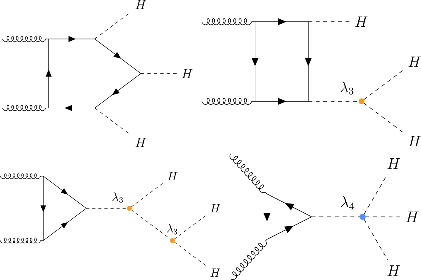
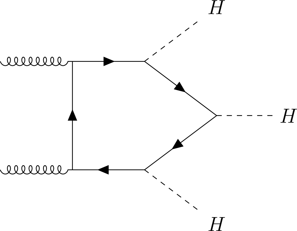
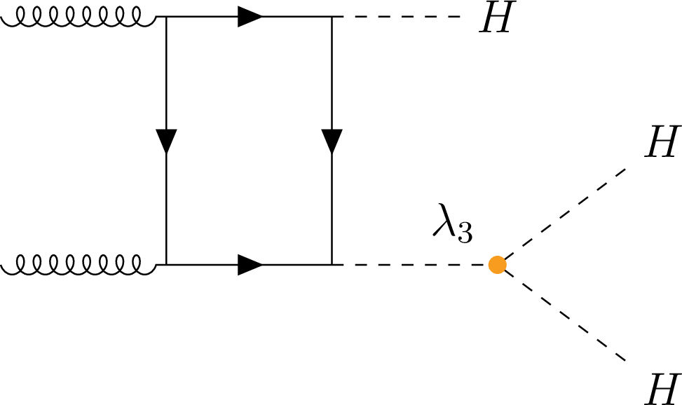
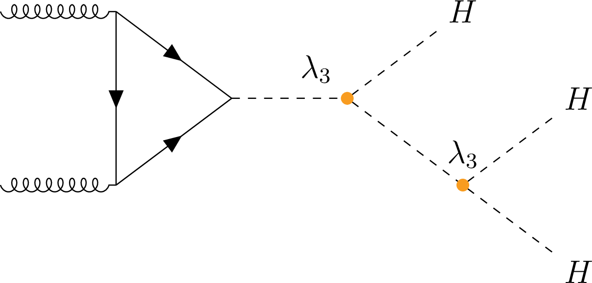
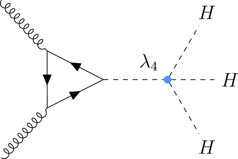
png pdf	Figure 1: Representative Feynman diagrams for HHH production via gluon-gluon fusion mode at LO. The vertices having contributions for $ \lambda_3 $ and $ \lambda_4 $ are marked in orange and blue, respectively.
png pdf	Figure 1-a: Representative Feynman diagrams for HHH production via gluon-gluon fusion mode at LO. The vertices having contributions for $ \lambda_3 $ and $ \lambda_4 $ are marked in orange and blue, respectively.
png pdf	Figure 1-b: Representative Feynman diagrams for HHH production via gluon-gluon fusion mode at LO. The vertices having contributions for $ \lambda_3 $ and $ \lambda_4 $ are marked in orange and blue, respectively.
png pdf	Figure 1-c: Representative Feynman diagrams for HHH production via gluon-gluon fusion mode at LO. The vertices having contributions for $ \lambda_3 $ and $ \lambda_4 $ are marked in orange and blue, respectively.
png pdf	Figure 1-d: Representative Feynman diagrams for HHH production via gluon-gluon fusion mode at LO. The vertices having contributions for $ \lambda_3 $ and $ \lambda_4 $ are marked in orange and blue, respectively.
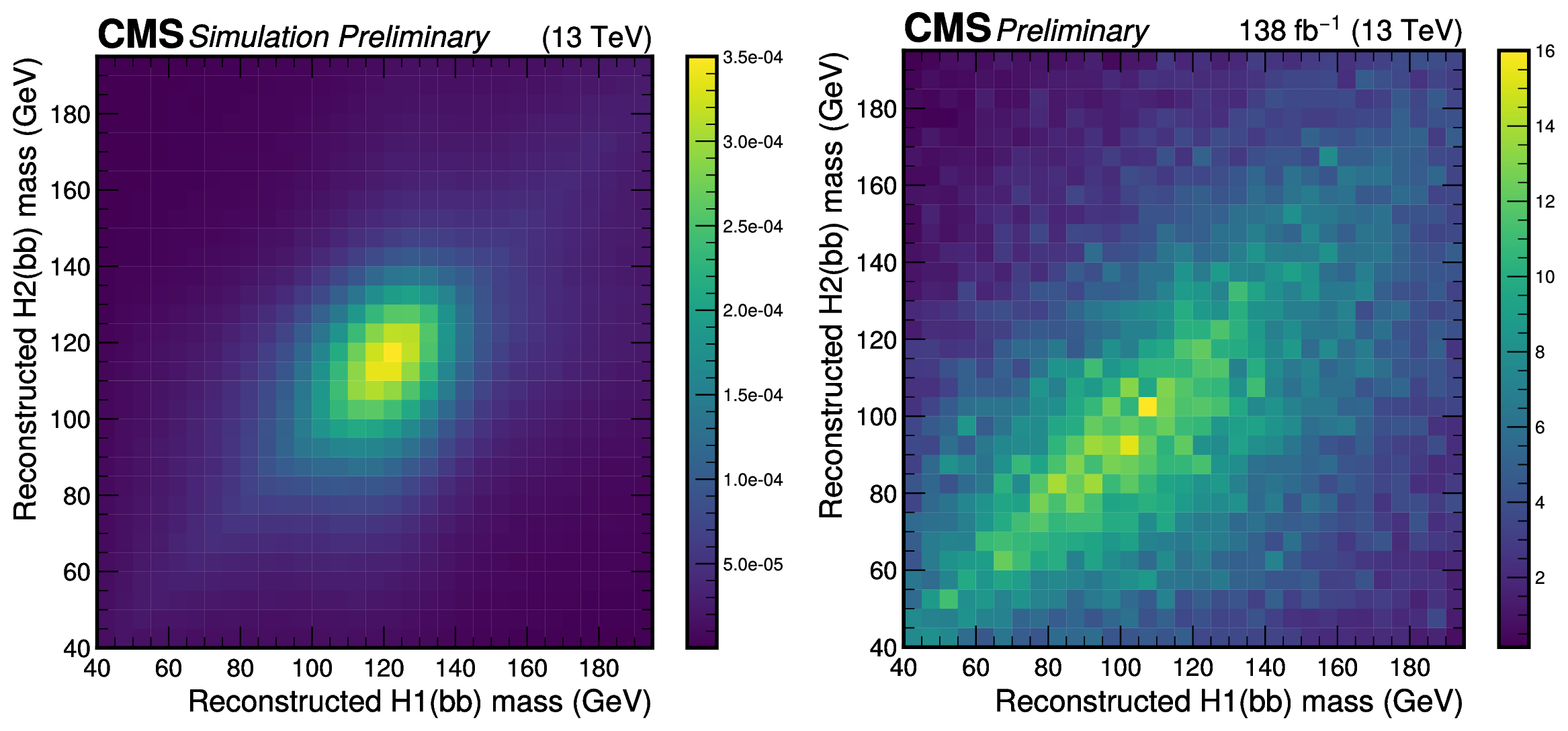
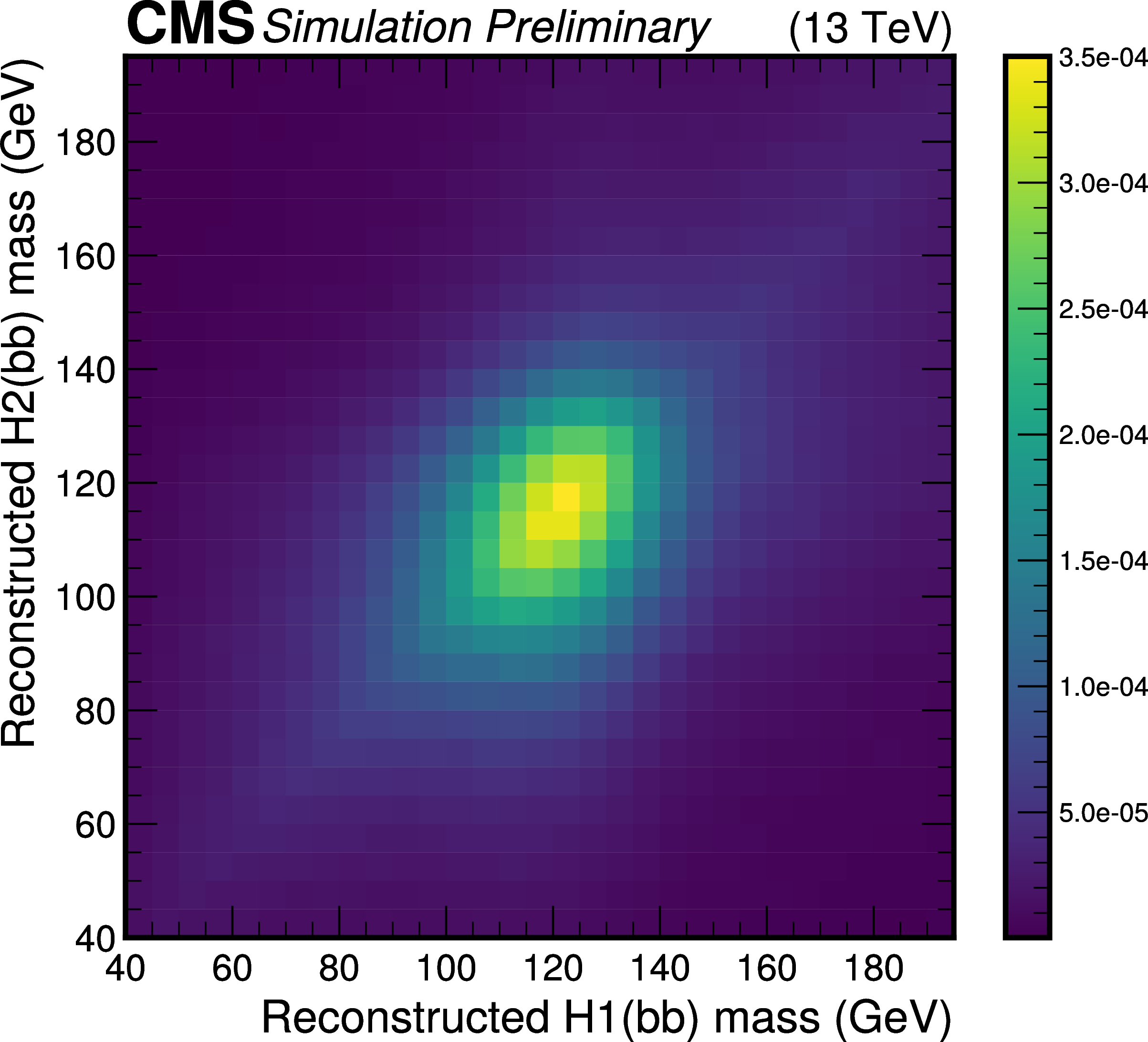
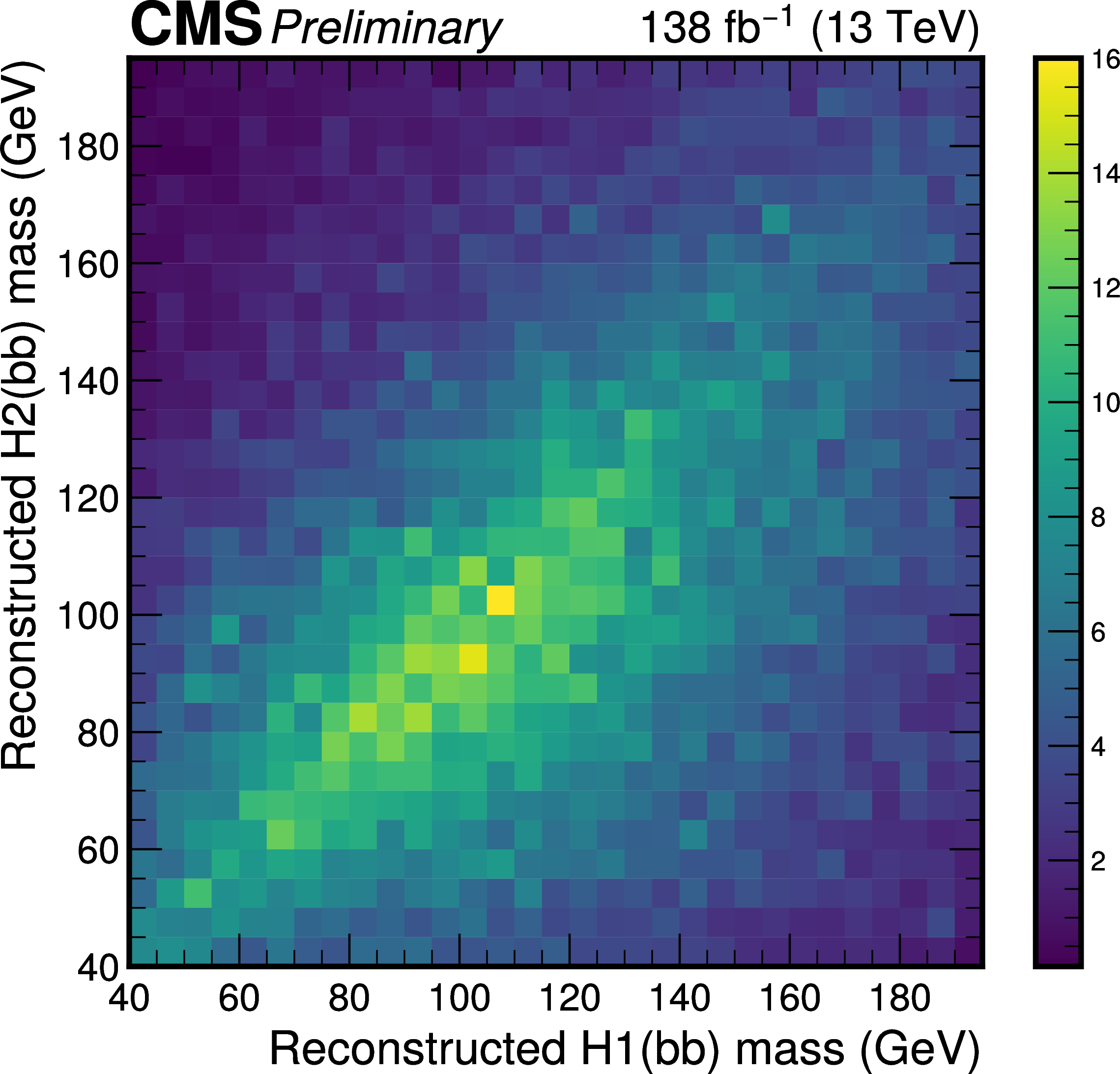
png pdf	Figure 2: Distributions of the reconstructed masses of the leading (H1) and subleading (H2) $ \mathrm{H}\to\mathrm{b}\overline{\mathrm{b}} $ candidates for signal events (left) and non-resonant backgrounds (right).
png pdf	Figure 2-a: Distributions of the reconstructed masses of the leading (H1) and subleading (H2) $ \mathrm{H}\to\mathrm{b}\overline{\mathrm{b}} $ candidates for signal events (left) and non-resonant backgrounds (right).
png pdf	Figure 2-b: Distributions of the reconstructed masses of the leading (H1) and subleading (H2) $ \mathrm{H}\to\mathrm{b}\overline{\mathrm{b}} $ candidates for signal events (left) and non-resonant backgrounds (right).
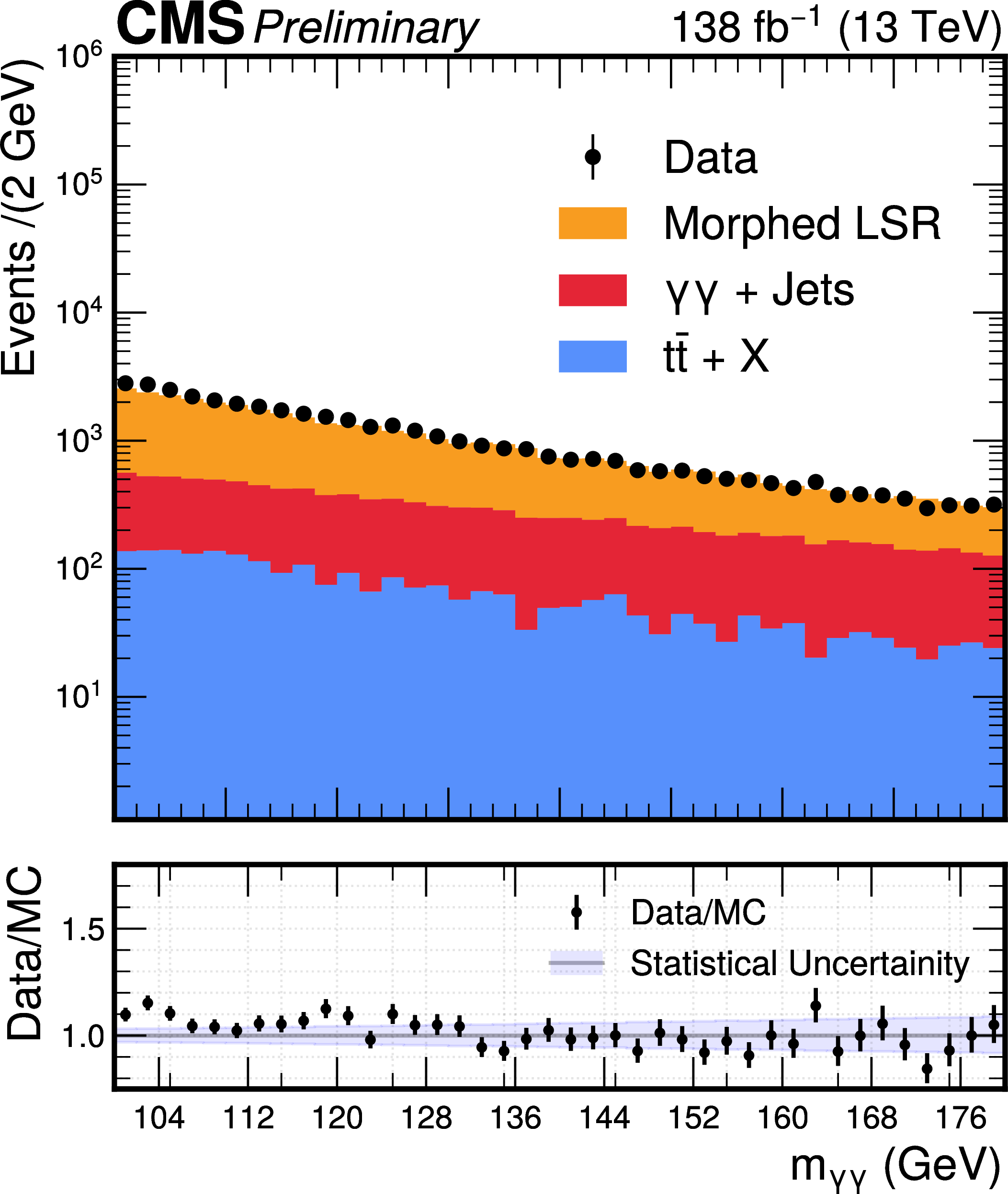
png pdf	Figure 3: Distribution of the reconstructed diphoton invariant mass in data (black points) and the predicted backgrounds (colored histograms) after event morphing. The vertical bars on the data points represent the statistical uncertainties associated with the data. The lower panel shows the ratio of data to the sum of background predictions. The light blue band in the lower panel represents the statistical uncertainty in the background predictions.
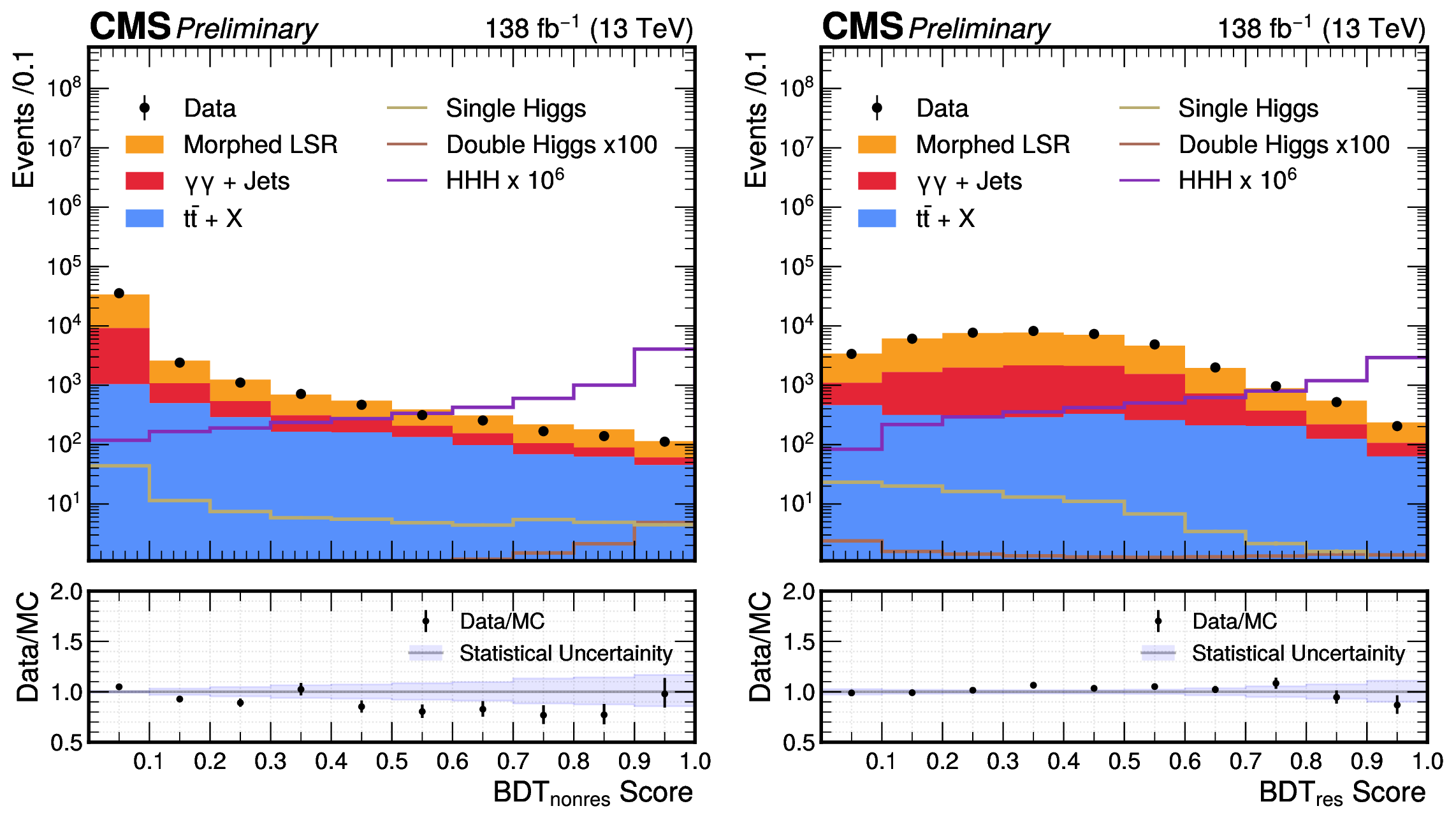
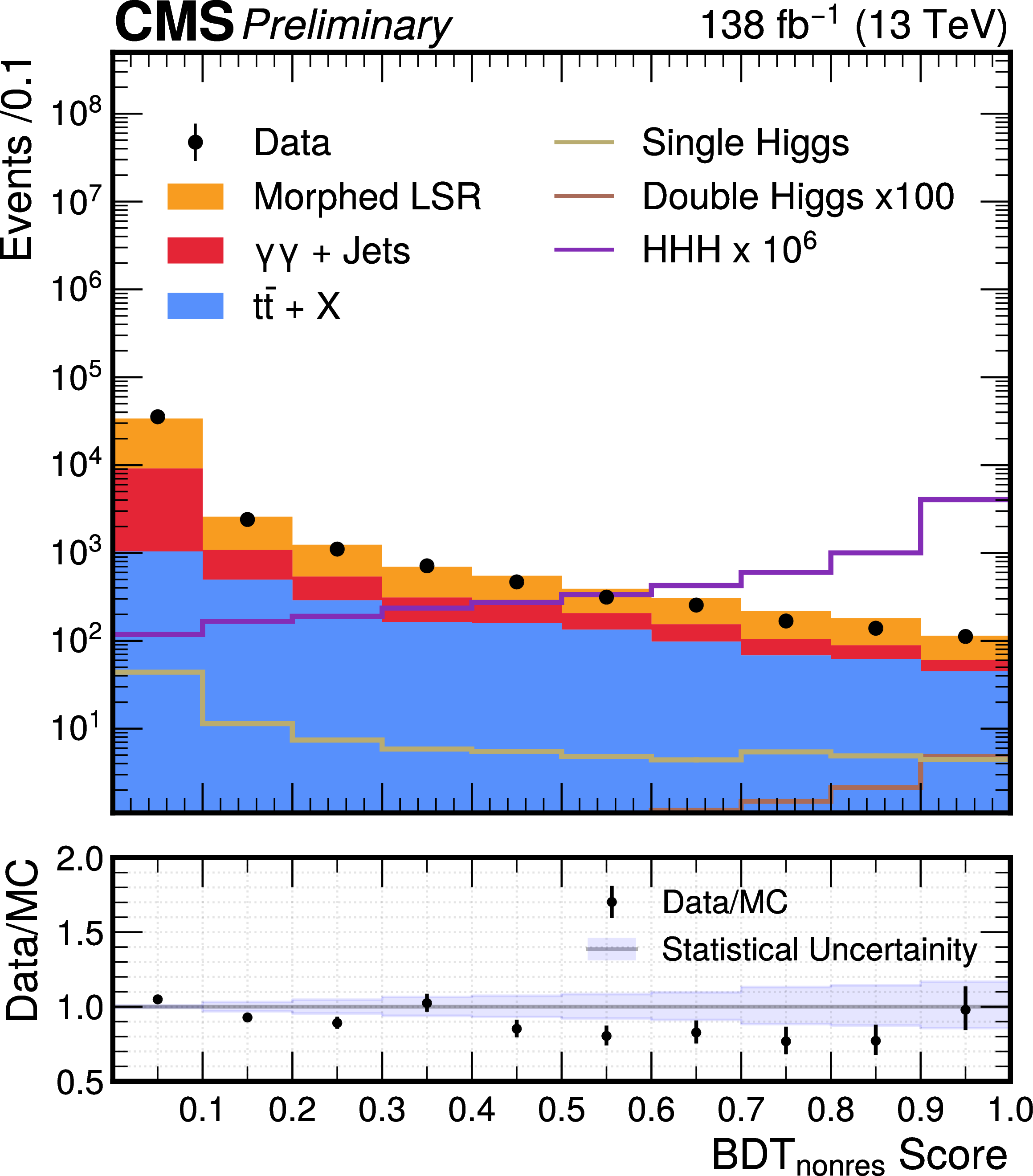
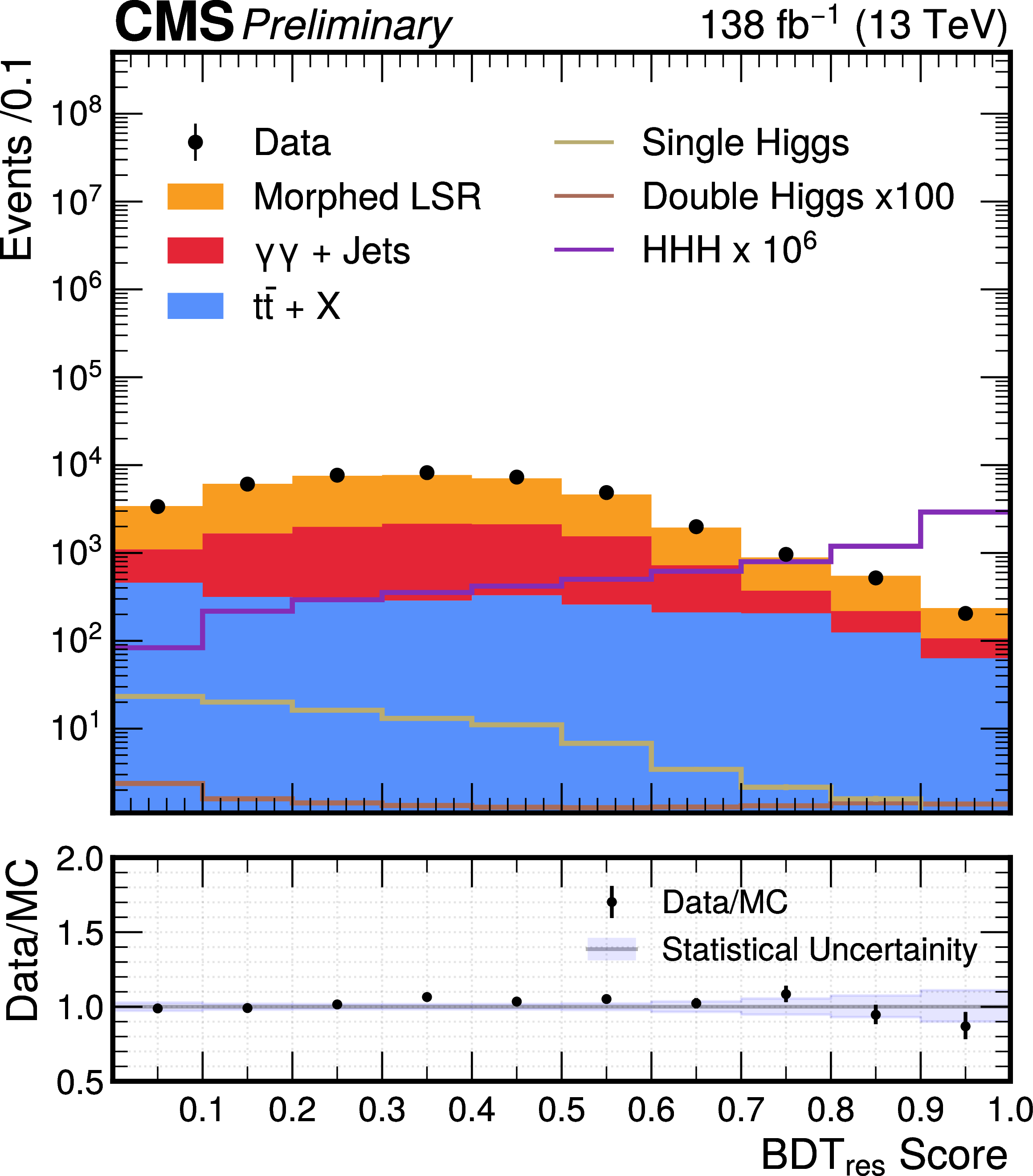
png pdf	Figure 4: Distribution of the BDT$ _{\text{nonres}} $ (left) and BDT$ _{\text{res}} $ (right) scores in data (black points) and predicted signal and backgrounds (colored histograms) after event morphing. The vertical error bars on the data points represent the statistical uncertainties in data. The violet line represents the expected distribution of signal HHH events, scaled by a factor of 10$ ^6 $. The lower panel shows the ratio of data to the sum of background predictions. The light blue band in the lower panel represents the statistical uncertainty in the background predictions. The imperfect description of the data by the simulation is not a concern in this context, as the scores from simulation are used solely for optimizing selections. The final background model for the non-resonant component is derived directly from the data. A highly magnified distribution due to the HH signal has been superposed for illustration.
png pdf	Figure 4-a: Distribution of the BDT$ _{\text{nonres}} $ (left) and BDT$ _{\text{res}} $ (right) scores in data (black points) and predicted signal and backgrounds (colored histograms) after event morphing. The vertical error bars on the data points represent the statistical uncertainties in data. The violet line represents the expected distribution of signal HHH events, scaled by a factor of 10$ ^6 $. The lower panel shows the ratio of data to the sum of background predictions. The light blue band in the lower panel represents the statistical uncertainty in the background predictions. The imperfect description of the data by the simulation is not a concern in this context, as the scores from simulation are used solely for optimizing selections. The final background model for the non-resonant component is derived directly from the data. A highly magnified distribution due to the HH signal has been superposed for illustration.
png pdf	Figure 4-b: Distribution of the BDT$ _{\text{nonres}} $ (left) and BDT$ _{\text{res}} $ (right) scores in data (black points) and predicted signal and backgrounds (colored histograms) after event morphing. The vertical error bars on the data points represent the statistical uncertainties in data. The violet line represents the expected distribution of signal HHH events, scaled by a factor of 10$ ^6 $. The lower panel shows the ratio of data to the sum of background predictions. The light blue band in the lower panel represents the statistical uncertainty in the background predictions. The imperfect description of the data by the simulation is not a concern in this context, as the scores from simulation are used solely for optimizing selections. The final background model for the non-resonant component is derived directly from the data. A highly magnified distribution due to the HH signal has been superposed for illustration.
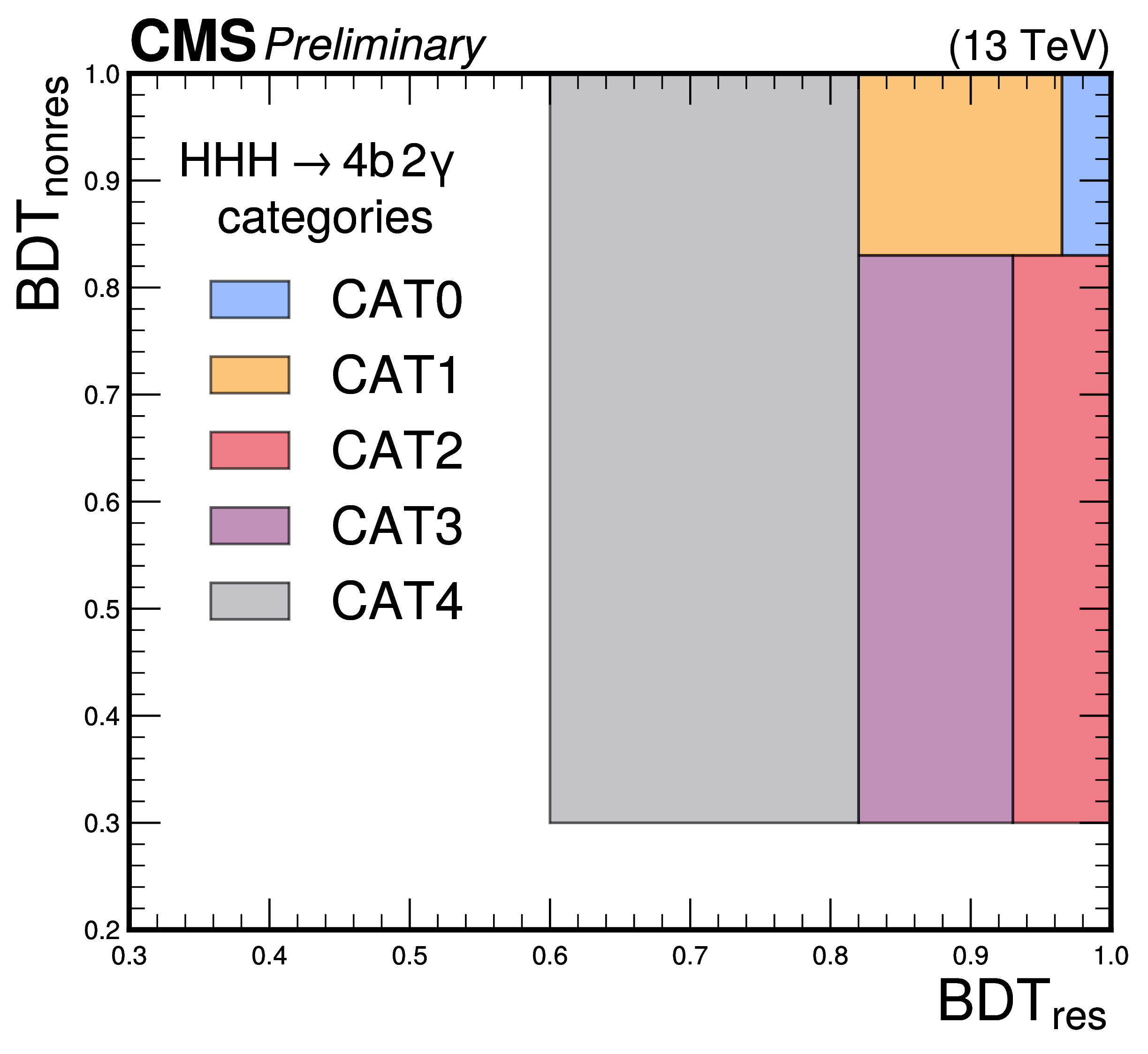
png pdf	Figure 5: Schematic representation of the analysis category definition in the two-dimensional plane of BDT$ _{\text{nonres}} $ and BDT$ _{\text{res}} $.
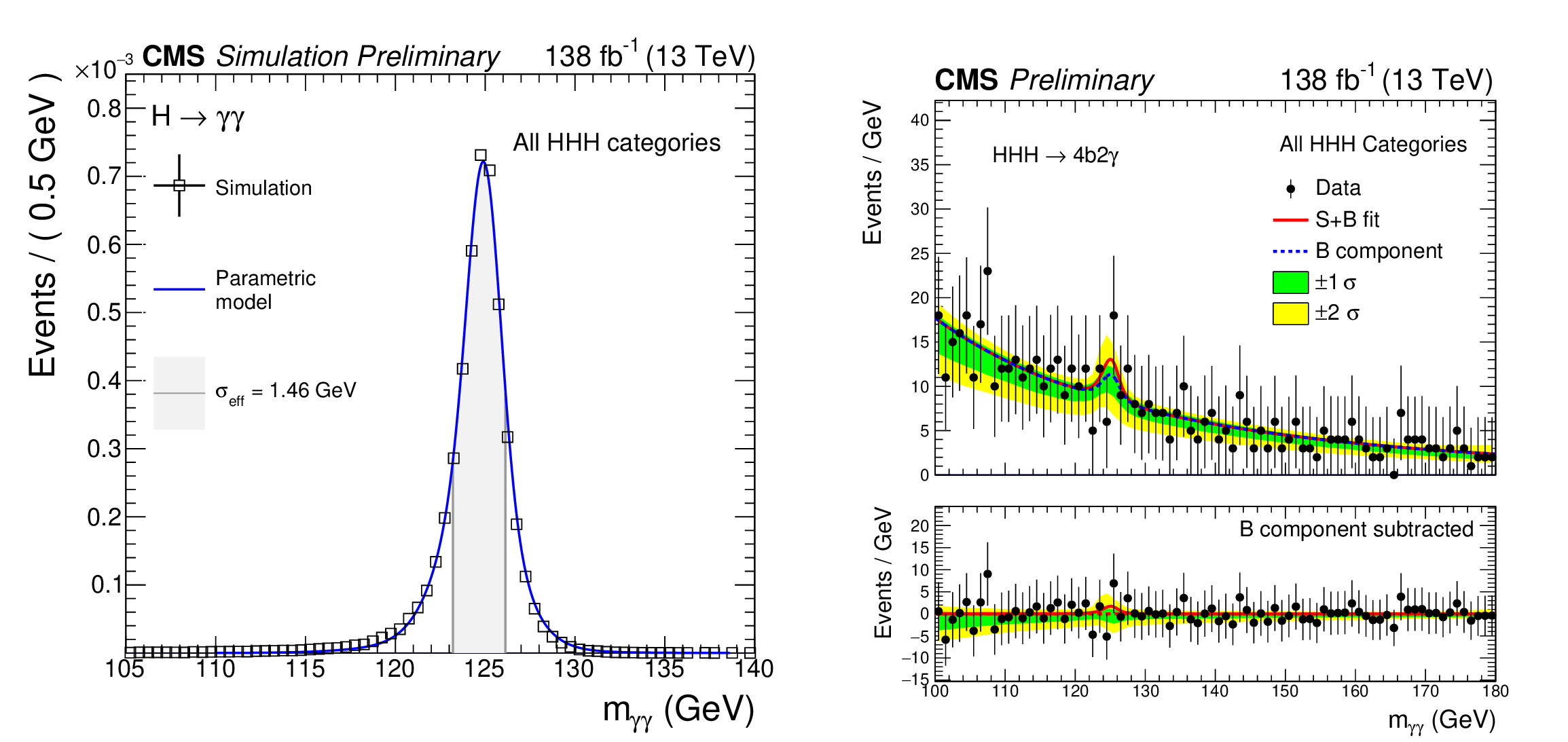
png pdf	Figure 6: Left: Parameterized signal shape for $ m_{\gamma\gamma} $. The open squares represent the simulated events and the blue lines are corresponding models. The corresponding interval as a gray band shows the $ \sigma_{\text{eff}} $ value (half the width of the narrowest interval containing 68.3% of the invariant mass distribution). Right: Invariant mass distribution of $ m_{\gamma\gamma} $ for the selected events in data (black points) from all analysis categories. The solid red lines demonstrates the fitted signal plus background model and the blue dotted line shows the background component. The lower panel shows the residual post fit signal yield after the background subtraction from data.
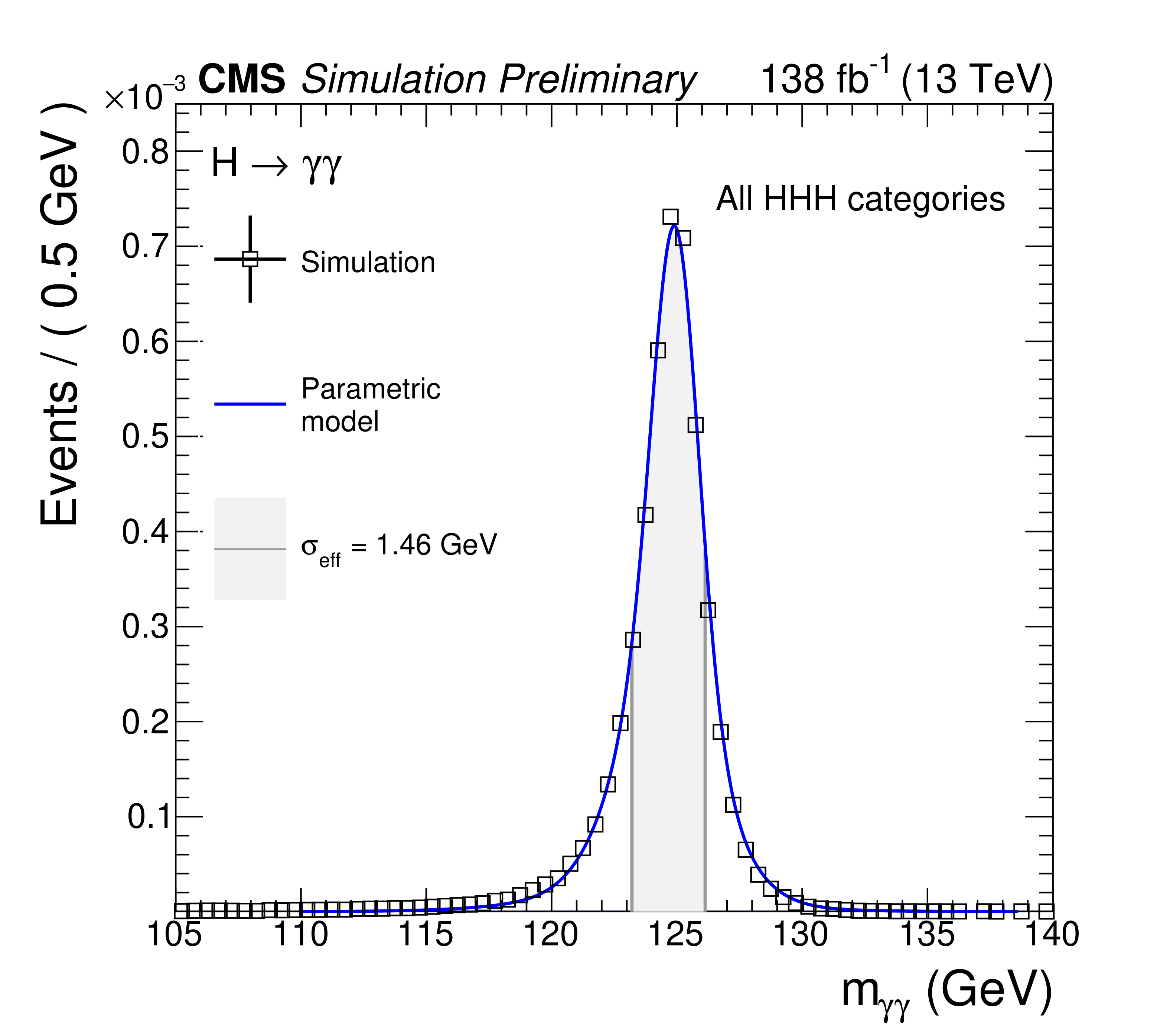
png pdf	Figure 6-a: Left: Parameterized signal shape for $ m_{\gamma\gamma} $. The open squares represent the simulated events and the blue lines are corresponding models. The corresponding interval as a gray band shows the $ \sigma_{\text{eff}} $ value (half the width of the narrowest interval containing 68.3% of the invariant mass distribution). Right: Invariant mass distribution of $ m_{\gamma\gamma} $ for the selected events in data (black points) from all analysis categories. The solid red lines demonstrates the fitted signal plus background model and the blue dotted line shows the background component. The lower panel shows the residual post fit signal yield after the background subtraction from data.
png pdf	Figure 6-b: Left: Parameterized signal shape for $ m_{\gamma\gamma} $. The open squares represent the simulated events and the blue lines are corresponding models. The corresponding interval as a gray band shows the $ \sigma_{\text{eff}} $ value (half the width of the narrowest interval containing 68.3% of the invariant mass distribution). Right: Invariant mass distribution of $ m_{\gamma\gamma} $ for the selected events in data (black points) from all analysis categories. The solid red lines demonstrates the fitted signal plus background model and the blue dotted line shows the background component. The lower panel shows the residual post fit signal yield after the background subtraction from data.
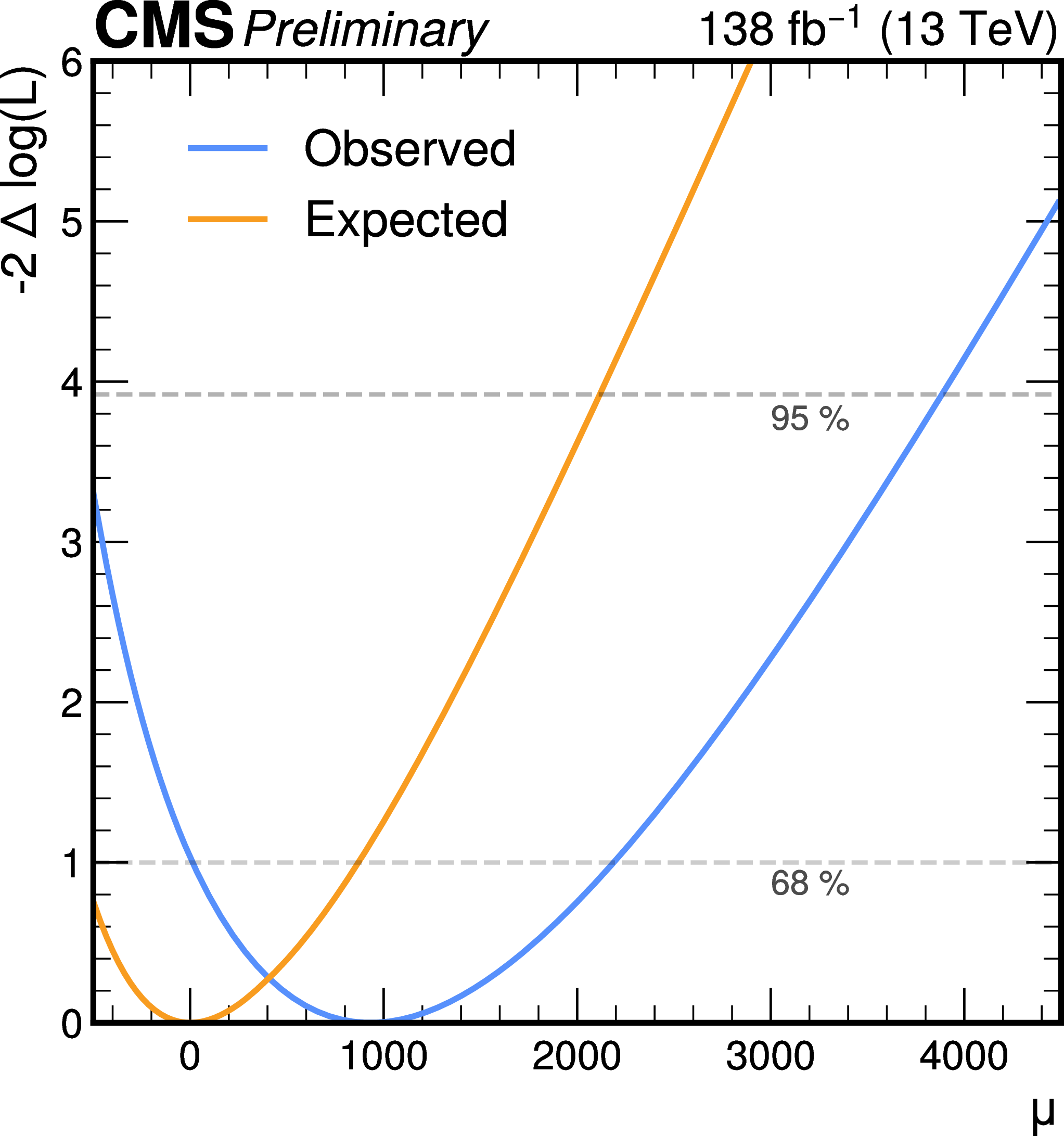
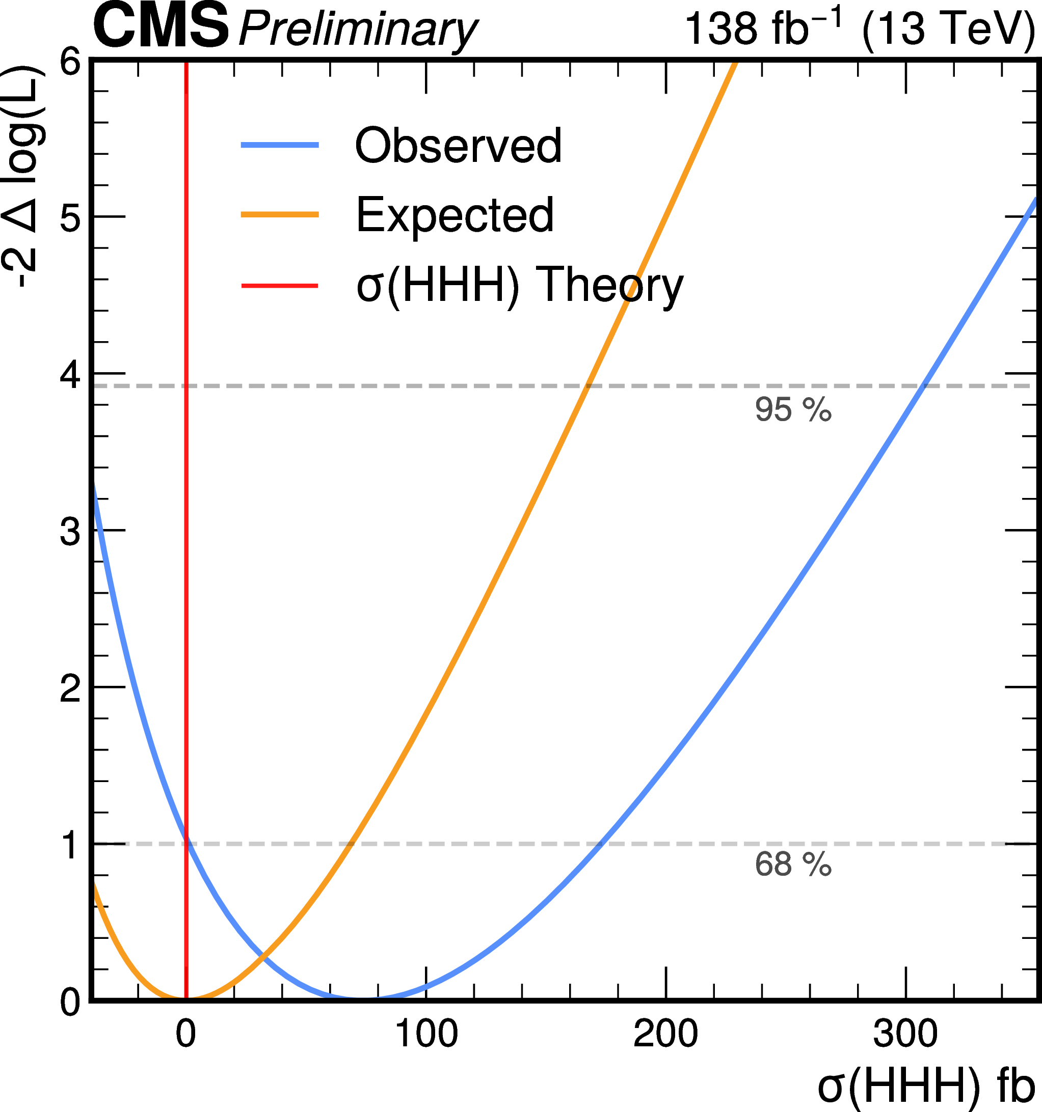
png pdf	Figure 7: Likelihood scan for the signal strength (left) and inclusive HHH crosssection (right). The blue and orange shows the observed and expected results respectively. The red line on the right plot shows the theoretical HHH crossection of 0.079 fb [11].
png pdf	Figure 7-a: Likelihood scan for the signal strength (left) and inclusive HHH crosssection (right). The blue and orange shows the observed and expected results respectively. The red line on the right plot shows the theoretical HHH crossection of 0.079 fb [11].
png pdf	Figure 7-b: Likelihood scan for the signal strength (left) and inclusive HHH crosssection (right). The blue and orange shows the observed and expected results respectively. The red line on the right plot shows the theoretical HHH crossection of 0.079 fb [11].
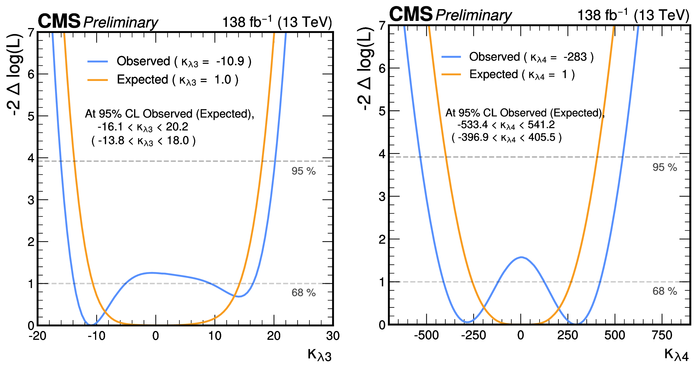
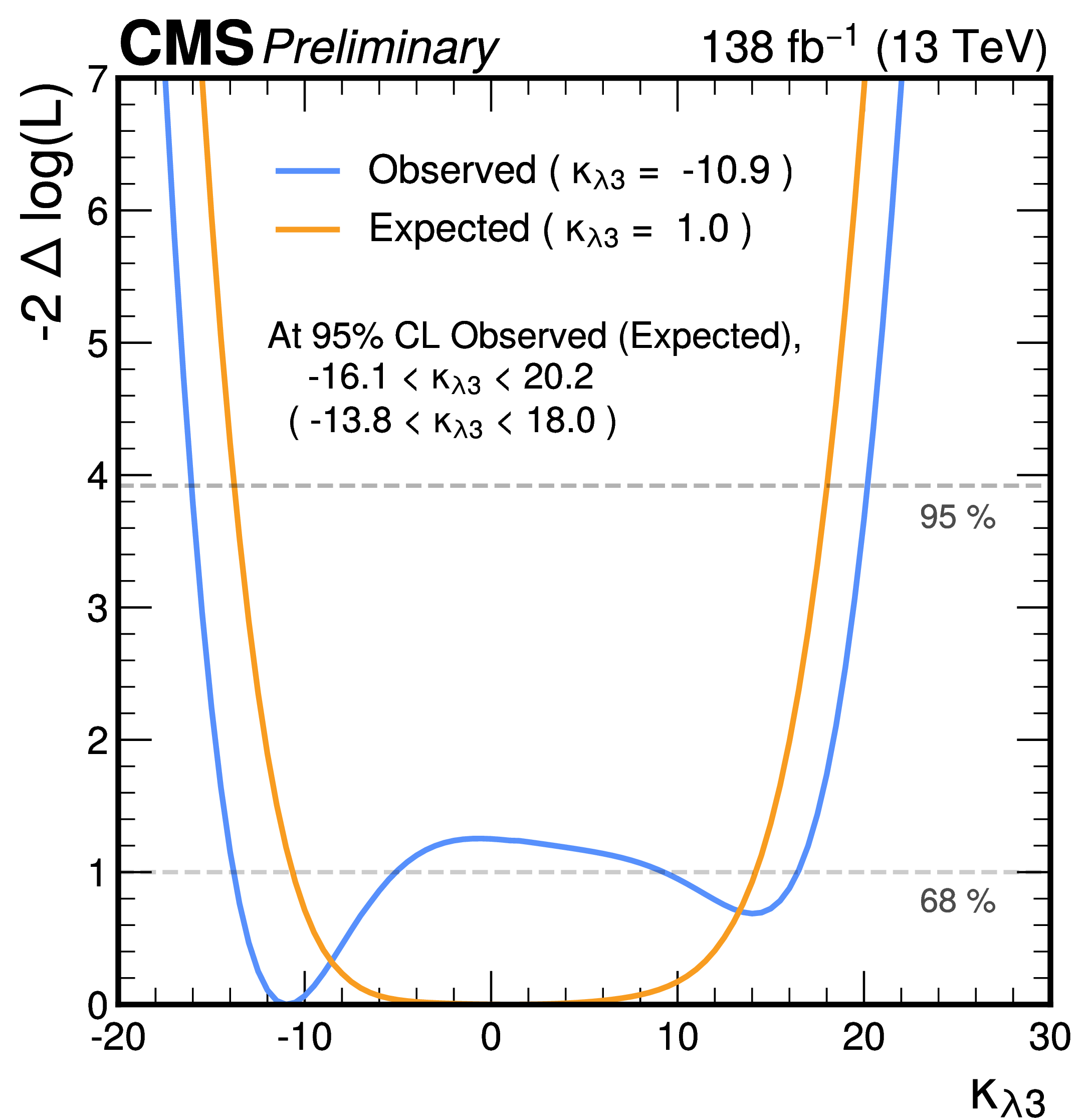
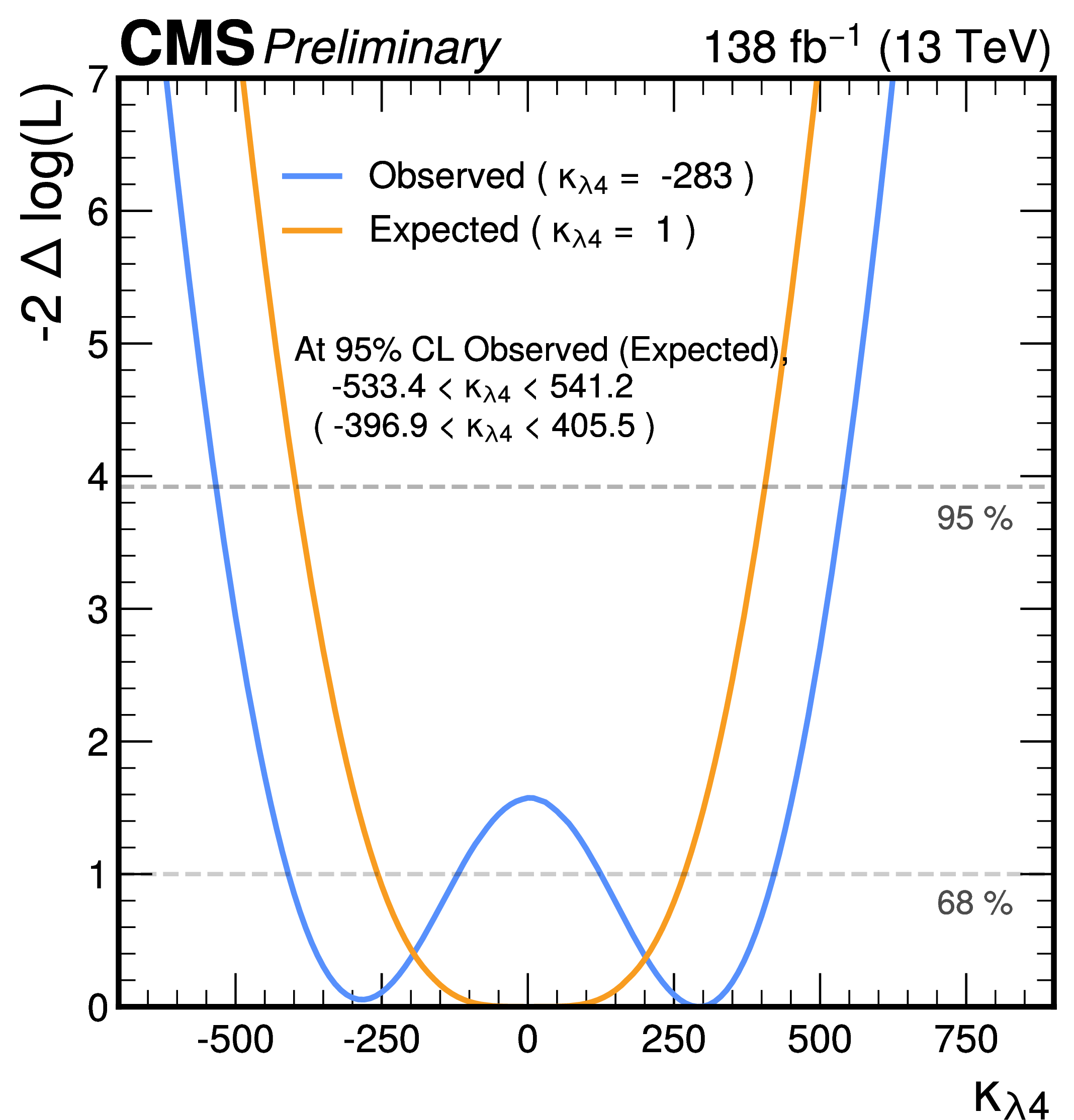
png pdf	Figure 8: Likelihood scan, as a function of $ \kappa_{\lambda 3} $ (left) and $ \kappa_{\lambda 4} $ (right). The blue and orange curves show the observed and expected results respectively. The 68% and 95% CL intervals are indicated by the horizontal dashed lines.
png pdf	Figure 8-a: Likelihood scan, as a function of $ \kappa_{\lambda 3} $ (left) and $ \kappa_{\lambda 4} $ (right). The blue and orange curves show the observed and expected results respectively. The 68% and 95% CL intervals are indicated by the horizontal dashed lines.
png pdf	Figure 8-b: Likelihood scan, as a function of $ \kappa_{\lambda 3} $ (left) and $ \kappa_{\lambda 4} $ (right). The blue and orange curves show the observed and expected results respectively. The 68% and 95% CL intervals are indicated by the horizontal dashed lines.
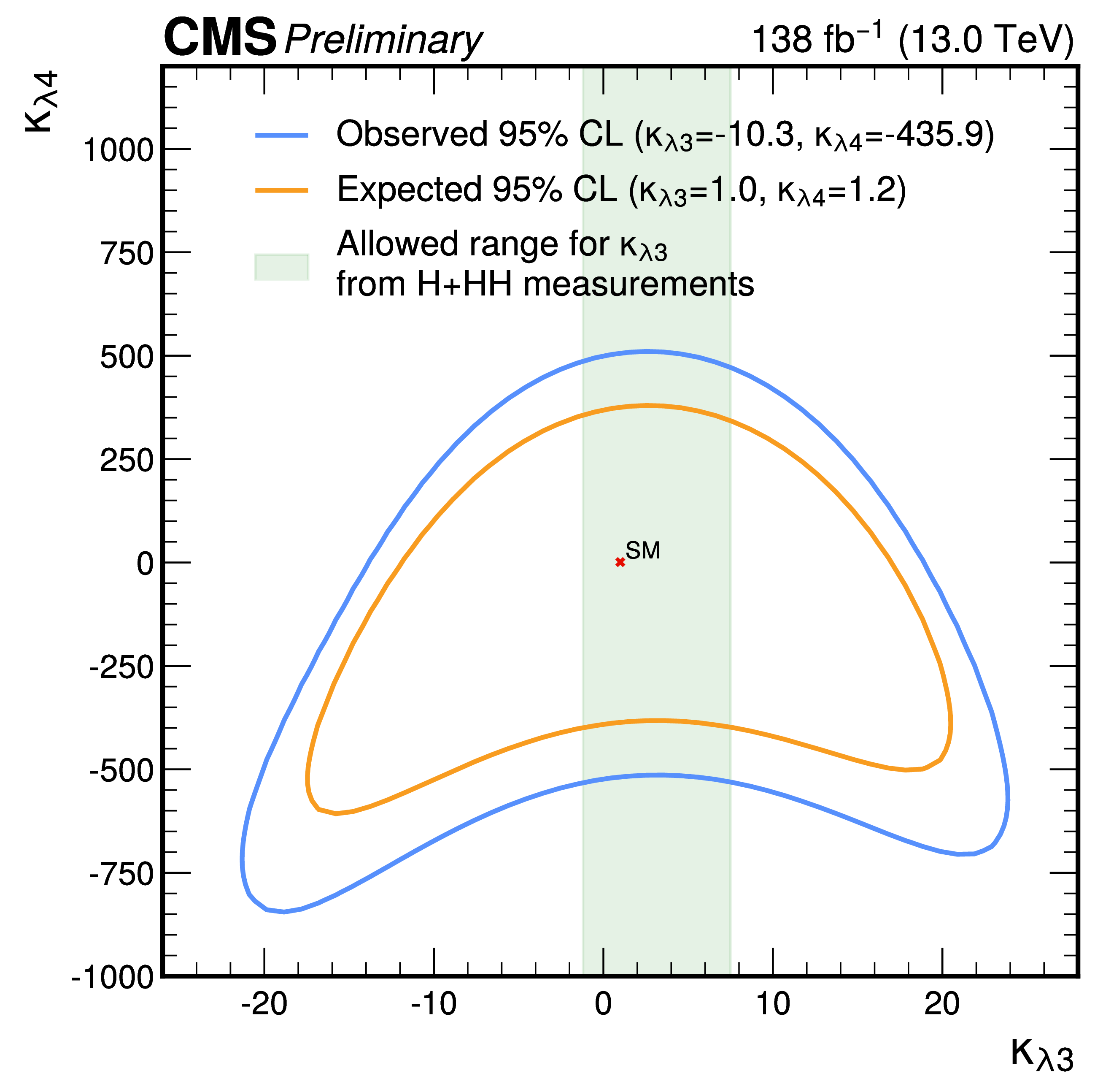
png pdf	Figure 9: Likelihood contours at 95% CL in the ($ \kappa_{\lambda 3} $, $ \kappa_{\lambda 4} $) plane evaluated with an Asimov data set assuming SM hypothesis (in orange line) and the observed data (in blue line). The green shaded region shows the allowed bounds on $ \kappa_{\lambda 3} $ from the H+HH combination measurements [9].

Summary

The first search for triple Higgs boson production (HHH) by the CMS collaboration has been presented, targeting the final state where two of the Higgs bosons decay to a pair of bottom quarks and one to a pair of photons. The search uses proton-proton collision data at $ \sqrt s $ = 13 TeV, corresponding to an integrated luminosity of 138 fb$ ^{-1} $. Upper limits on the product of the HHH production cross section and the $ \mathrm{HHH} \rightarrow4\mathrm{b}2\gamma $ branching fraction are extracted. The observed (expected) upper limit is 0.56 (0.35) fb at 95% confidence level (CL), corresponding to 3400 (2086) times the standard model cross section value. The results are interpreted in the $ \kappa $-framework, setting upper limits on the trilinear and quartic Higgs boson self-coupling modifiers $ \kappa_{\lambda 3} $ = $ \frac{\lambda_3}{\lambda_3^{SM}} $ and $ \kappa_{\lambda 4} $ = $ \frac{\lambda_4}{\lambda_4^{SM}} $ respectively, assuming that the top quark Yukawa coupling is standard model like. The trilinear self-coupling modifier $ \kappa_{\lambda 3} $ is observed (expected) to be constrained within a range of [$-$16.1,20.2] ([$-$13.8,18.0]) at 95% CL. The quartic self-coupling modifier $ \kappa_{\lambda 4} $ is observed (expected) to be constrained within a range of [$-$533,541] ( [$-$397,406] ) at 95% CL. The simultaneous constraints on the $ \kappa_{\lambda 3} $ and $ \kappa_{\lambda 4} $ has also been presented from the two-dimensional likelihood scan.

References
1	CMS Collaboration	A portrait of the Higgs boson by the CMS experiment ten years after the discovery.	Nature 607 (2022) 60	CMS-HIG-22-001 2207.00043
2	ATLAS Collaboration	A detailed map of Higgs boson interactions by the ATLAS experiment ten years after the discovery	Nature 607 (2022) 52	2207.00092
3	T. Robens, T. Stefaniak, and J. Wittbrodt	Two-real-scalar-singlet extension of the SM: LHC phenomenology and benchmark scenarios	EPJC 80 (2020) 151	1908.08554
4	T.-K. Chen, C.-W. Chiang, and I. Low	Simple model of dark matter and cp violation	Physical Review D 105 (2022)
5	H. Abouabid et al.	HHH whitepaper	EPJC 84 (2024) 1183	2407.03015
6	ATLAS Collaboration	Searches for Higgs boson pair production in the $ hh\to bb\tau\tau, \gamma\gamma WW^*, \gamma\gamma bb, bbbb $ channels with the ATLAS detector	PRD 92 (2015) 092004	1509.04670
7	CMS Collaboration	Search for Higgs boson pair production in the $ bb\tau\tau $ final state in proton-proton collisions at $ \sqrt{(}s)=8\text{ }\text{ }\mathrm{TeV} $	PRD 96 (2017) 072004	CMS-HIG-15-013 1707.00350
8	CMS Collaboration	Search for two Higgs bosons in final states containing two photons and two bottom quarks in proton-proton collisions at 8 TeV	PRD 94 (2016) 052012	CMS-HIG-13-032 1603.06896
9	CMS Collaboration	Constraints on the higgs boson self-coupling from the combination of single and double higgs boson production in proton-proton collisions at $ \sqrt{s} $ = 13 tev	link
10	ATLAS Collaboration Collaboration	Combination of searches for higgs boson pair production in $ pp $ collisions at $ \sqrt{s}=13\text{ }\text{ }\mathrm{TeV} $ with the atlas detector	PRL 133 (2024) 101801
11	D. de Florian, I. Fabre, and J. Mazzitelli	Triple Higgs production at hadron colliders at NNLO in QCD	JHEP 03 (2020) 155	1912.02760
12	ATLAS Collaboration	HL-LHC prospects for the measurement of triple-Higgs production in the 6b final state at the ATLAS experiment	technical report, CERN, ATL-PHYS-PUB-2025-003, 2025
13	CMS Collaboration	Precision luminosity measurement in proton-proton collisions at $ \sqrt{s} = $ 13 TeV in 2015 and 2016 at CMS	EPJC 81 (2021) 800	CMS-LUM-17-003 2104.01927
14	CMS Collaboration	The CMS Experiment at the CERN LHC	JINST 3 (2008) S08004
15	CMS Collaboration	Description and performance of track and primary-vertex reconstruction with the CMS tracker	JINST 9 (2014) P10009	CMS-TRK-11-001 1405.6569
16	CMS Collaboration	Performance of the CMS Level-1 trigger in proton-proton collisions at $ \sqrt{s} = $ 13 TeV	JINST 15 (2020) P10017	CMS-TRG-17-001 2006.10165
17	CMS Collaboration	The CMS trigger system	JINST 12 (2017) P01020	CMS-TRG-12-001 1609.02366
18	CMS Collaboration	Measurements of Higgs boson properties in the diphoton decay channel in proton-proton collisions at $ \sqrt{s} = $ 13 TeV	JHEP 11 (2018) 185	CMS-HIG-16-040 1804.02716
19	J. Alwall et al.	The automated computation of tree-level and next-to-leading order differential cross sections, and their matching to parton shower simulations	JHEP 07 (2014) 079	1405.0301
20	P. Nason and C. Oleari	NLO Higgs boson production via vector-boson fusion matched with shower in POWHEG	JHEP 02 (2010) 037	0911.5299
21	T. Sjöstrand et al.	An introduction to PYTHIA8.2	Comput. Phys. Commun. 191 (2015) 159	1410.3012
22	T. Gleisberg et al.	Event generation with SHERPA 1.1	JHEP 02 (2009) 007	0811.4622
23	CMS Collaboration	Event generator tunes obtained from underlying event and multiparton scattering measurements	EPJC 76 (2016) 155	CMS-GEN-14-001 1512.00815
24	CMS Collaboration	Extraction and validation of a new set of CMS PYTHIA8 tunes from underlying-event measurements	EPJC 80 (2020) 4	CMS-GEN-17-001 1903.12179
25	R. D. Ball et al.	Parton distributions from high-precision collider data: Nnpdf collaboration	The European Physical Journal C 77 (2017)
26	GEANT4 Collaboration	GEANT4---a simulation toolkit	NIM A 506 (2003) 250
27	M. Cacciari, G. P. Salam, and G. Soyez	The anti-$ k_{\mathrm{T}} $ jet clustering algorithm	JHEP 04 (2008) 063	0802.1189
28	M. Cacciari, G. P. Salam, and G. Soyez	FastJet user manual	EPJC 72 (2012) 1896	1111.6097
29	CMS Collaboration	Electron and photon reconstruction and identification with the CMS experiment at the CERN LHC	JINST 16 (2021) P05014	CMS-EGM-17-001 2012.06888
30	CMS Collaboration	Search for Higgs Boson Pair Production in the Four b Quark Final State in Proton-Proton Collisions at s=13\,\,TeV	PRL 129 (2022) 081802	CMS-HIG-20-005 2202.09617
31	E. Bols et al.	Jet Flavour Classification Using DeepJet	JINST 15 (2020) P12012	2008.10519
32	CMS Collaboration	Performance of the DeepJet b tagging algorithm using 41.9 fb$ ^{-1} $ of data from proton-proton collisions at 13 TeV with Phase 1 CMS detector	CMS Detector Performance Note CMS-DP-2018-058, 2018 CDS
33	CMS Collaboration	Measurements of $ \mathrm{t\bar{t}}H $ Production and the CP Structure of the Yukawa Interaction between the Higgs Boson and Top Quark in the Diphoton Decay Channel	PRL 125 (2020) 061801	CMS-HIG-19-013 2003.10866
34	T. Chen and C. Guestrin	Xgboost: A scalable tree boosting system	in Proceedings of the 22nd ACM SIGKDD International Conference on Knowledge Discovery and Data Mining, KDD '16. ACM, 2016 link
35	C. Adam-Bourdarios et al.	The higgs machine learning challenge	Journal of Physics, 2015 Conference Series 664 (2015) 072015
36	G. Cowan, K. Cranmer, E. Gross, and O. Vitells	Asymptotic formulae for likelihood-based tests of new physics	The European Physical Journal C 71 (2011)
37	CMS Collaboration	Search for the associated production of the higgs boson with a top-quark pair	Journal of High Energy Physics 2014 (2014) 87
38	CMS Collaboration	CMS luminosity measurement for the 2017 data-taking period at $ \sqrt{s} = $ 13 TeV	technical report, CERN, Geneva, 2018 CDS
39	CMS Collaboration	CMS luminosity measurement for the 2018 data-taking period at $ \sqrt{s} = $ 13 TeV	technical report, CERN, Geneva, 2019 CDS
40	CMS Collaboration	The CMS Statistical Analysis and Combination Tool: Combine	Comput. Softw. Big Sci. 8 (2024) 19	CMS-CAT-23-001 2404.06614