CMS-PAS-FTR-21-002

CMS-PAS-FTR-21-002
Prospects for the measurement of $\mathrm{t\bar{t}}$H production in the opposite-sign dilepton channel at $\sqrt{s}$ = 14 TeV at the High-Luminosity LHC
CMS Collaboration
March 2022

Abstract: Prospects for the measurement of top quark-antiquark associated Higgs boson ($\mathrm{t\bar{t}}$H) production in the HL-LHC era are presented. The measurement is performed in the opposite sign dilepton channel where $e^{+}e^{-}$, $\mu^{+}\mu^{-}$ and $e^{\pm}\mu^{\pm}$ are considered, while focusing on the H $ \to \mathrm{b\bar{b}}$ decay. A novel approach with respect to previous analyses and the projection study for the HL-LHC is explored. The analysis strategy is based on the reconstruction of the Higgs boson invariant mass through the analytical solution of the kinematic equations of the $\mathrm{t\bar{t}}$H system, employs a neural network for the selection of data and makes use of a data-based method to estimate the main backgrounds. The results are extrapolated to the full integrated luminosity expected at the High-Luminosity LHC at $\sqrt{s}=$ 14 TeV, with the signal strength being expected to be extracted with $^{+0.13}_{-0.12}$ uncertainty.
Links: CDS record (PDF) ; CADI line (restricted) ;

Figures & Tables	Summary	References	CMS Publications

Figures
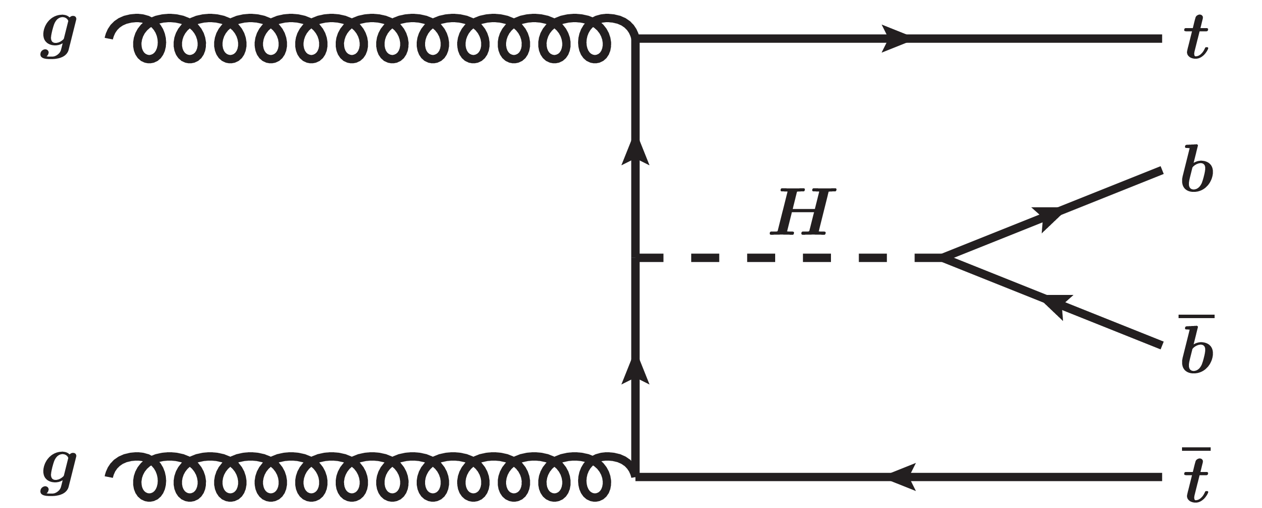
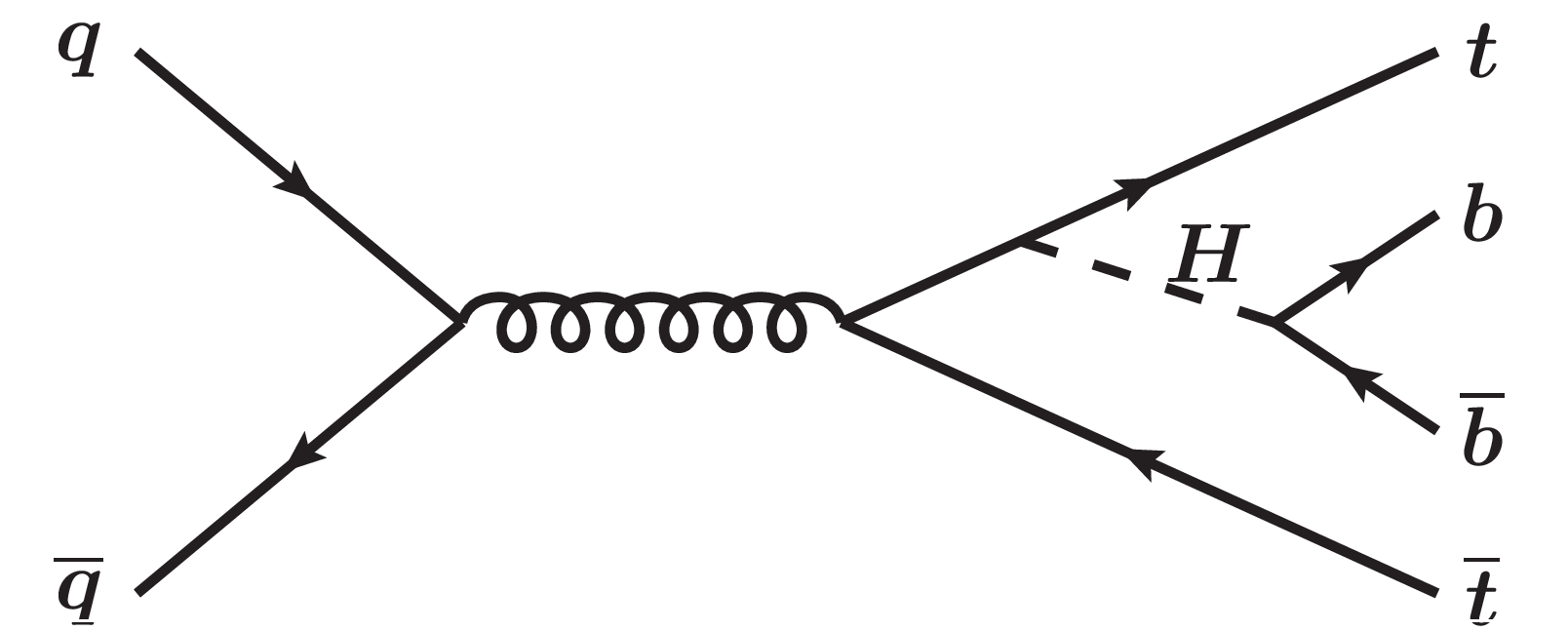
png pdf	Figure 1: Tree-level Feynman diagrams for the production of a Higgs boson in association with a top quark-antiquark pair ($\mathrm{t\bar{t}}$H) in the t-channel (left) and in the s-channel (right). In both cases the Higgs boson subsequently decays to a pair of b and anti-b quarks (H $ \to \mathrm{b\bar{b}}$).
png pdf	Figure 1-a: Tree-level Feynman diagrams for the production of a Higgs boson in association with a top quark-antiquark pair ($\mathrm{t\bar{t}}$H) in the t-channel (left) and in the s-channel (right). In both cases the Higgs boson subsequently decays to a pair of b and anti-b quarks (H $ \to \mathrm{b\bar{b}}$).
png	Figure 1-b: Tree-level Feynman diagrams for the production of a Higgs boson in association with a top quark-antiquark pair ($\mathrm{t\bar{t}}$H) in the t-channel (left) and in the s-channel (right). In both cases the Higgs boson subsequently decays to a pair of b and anti-b quarks (H $ \to \mathrm{b\bar{b}}$).
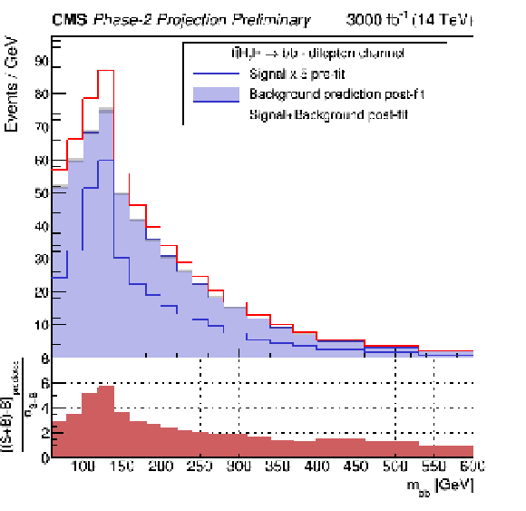
png pdf	Figure 2: Reconstructed invariant mass ${m_{\mathrm{b\bar{b}}}}$ distribution in the signal region after the fit to Asimov data. The expected signal+background distribution is shown with a red line and is constructed using simulated events in the signal region at $\sqrt {s} = $14 TeV scaled to an integrated luminosity of 3000 fb$^{-1}$. The background prediction has been extrapolated to the signal region using events in the control region by applying event probability weights. The post-fit background prediction distribution is shown with a filled purple histogram. The pre-fit $\mathrm{t\bar{t}}$H signal distribution, multiplied by a factor 5, is overlayed with a blue line. The bottom panel shows the pull distribution defined as the per-bin ratio of the expected number of data minus the expected number of background events over the per-bin statistical uncertainty of the expected data.
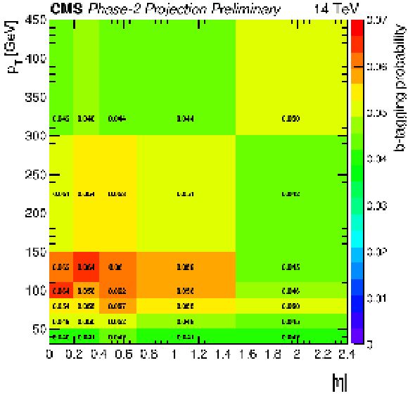
png pdf	Figure 3: B-tagging probability map as a function of ${p_{\text {T}}}$ and $\eta $.
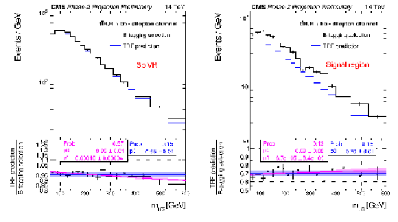
png pdf	Figure 4: Left: The ${m_{\mathrm{b\bar{b}}}}$ distribution is shown for $\mathrm{t\bar{t}} $+jets events in the 3b VR when applying the b-tagging selection (black) and when applying TRF weights to events in the 2b CR to predict the distribution in the 3b VR (blue) while the bottom panel shows the ratio of these two distributions (black points). The ratio has been fitted with a polynomial function of 0$^{th}$ degree (blue line) and of 1$^{st}$ degree (magenta line). The fitted parameter values of the 0$^{th}$ (1$^{st}$) degree polynomials are shown in the blue (magenta) box. The goodness-of-fit is assessed by a chi-square test, the probability of which is also denoted. Right: The ${m_{\mathrm{b\bar{b}}}}$ distribution is shown for $\mathrm{t\bar{t}} $+jets events in the SR when applying the b-tagging selection (black) and when applying TRF weights to events in the 2b CR to predict the distribution in the SR (blue) while the bottom panel shows the ratio of these two distributions (black points). The ratio has been fitted with a polynomial function of 0$^{th}$ degree (blue line) and of 1$^{st}$ degree (magenta line). The fitted parameter values of the 0$^{th}$ (1$^{st}$) degree polynomials are shown in the blue (magenta) box. The goodness-of-fit is assessed by a chi-square test, the probability of which is also denoted.
png	Figure 4-a: Left: The ${m_{\mathrm{b\bar{b}}}}$ distribution is shown for $\mathrm{t\bar{t}} $+jets events in the 3b VR when applying the b-tagging selection (black) and when applying TRF weights to events in the 2b CR to predict the distribution in the 3b VR (blue) while the bottom panel shows the ratio of these two distributions (black points). The ratio has been fitted with a polynomial function of 0$^{th}$ degree (blue line) and of 1$^{st}$ degree (magenta line). The fitted parameter values of the 0$^{th}$ (1$^{st}$) degree polynomials are shown in the blue (magenta) box. The goodness-of-fit is assessed by a chi-square test, the probability of which is also denoted. Right: The ${m_{\mathrm{b\bar{b}}}}$ distribution is shown for $\mathrm{t\bar{t}} $+jets events in the SR when applying the b-tagging selection (black) and when applying TRF weights to events in the 2b CR to predict the distribution in the SR (blue) while the bottom panel shows the ratio of these two distributions (black points). The ratio has been fitted with a polynomial function of 0$^{th}$ degree (blue line) and of 1$^{st}$ degree (magenta line). The fitted parameter values of the 0$^{th}$ (1$^{st}$) degree polynomials are shown in the blue (magenta) box. The goodness-of-fit is assessed by a chi-square test, the probability of which is also denoted.
png	Figure 4-b: Left: The ${m_{\mathrm{b\bar{b}}}}$ distribution is shown for $\mathrm{t\bar{t}} $+jets events in the 3b VR when applying the b-tagging selection (black) and when applying TRF weights to events in the 2b CR to predict the distribution in the 3b VR (blue) while the bottom panel shows the ratio of these two distributions (black points). The ratio has been fitted with a polynomial function of 0$^{th}$ degree (blue line) and of 1$^{st}$ degree (magenta line). The fitted parameter values of the 0$^{th}$ (1$^{st}$) degree polynomials are shown in the blue (magenta) box. The goodness-of-fit is assessed by a chi-square test, the probability of which is also denoted. Right: The ${m_{\mathrm{b\bar{b}}}}$ distribution is shown for $\mathrm{t\bar{t}} $+jets events in the SR when applying the b-tagging selection (black) and when applying TRF weights to events in the 2b CR to predict the distribution in the SR (blue) while the bottom panel shows the ratio of these two distributions (black points). The ratio has been fitted with a polynomial function of 0$^{th}$ degree (blue line) and of 1$^{st}$ degree (magenta line). The fitted parameter values of the 0$^{th}$ (1$^{st}$) degree polynomials are shown in the blue (magenta) box. The goodness-of-fit is assessed by a chi-square test, the probability of which is also denoted.
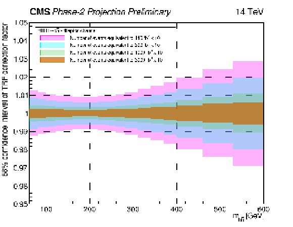
png pdf	Figure 5: The 68% confidence level uncertainty bands of the 1$^{st}$ degree polynomial used to correct the background prediction is shown as a function of the reconstructed $m_{\mathrm{b\bar{b}}}$ invariant mass. The number of events in simulation is assumed to be 10 times larger than the one expected in data. The progression of the uncertainty bands is shown for 140 fb$^{-1}$ x 10 (pink), 300 fb$^{-1}$ x 10 (light blue), 1000 fb$^{-1}$ x 10 (green) and 3000 fb$^{-1}$ x 10 (brown) of simulated events.
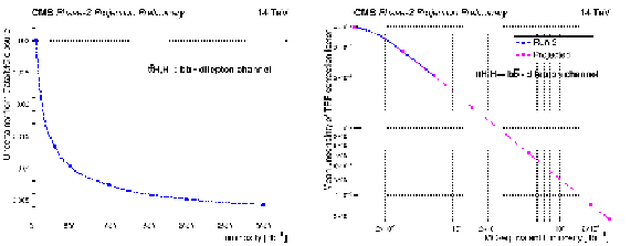
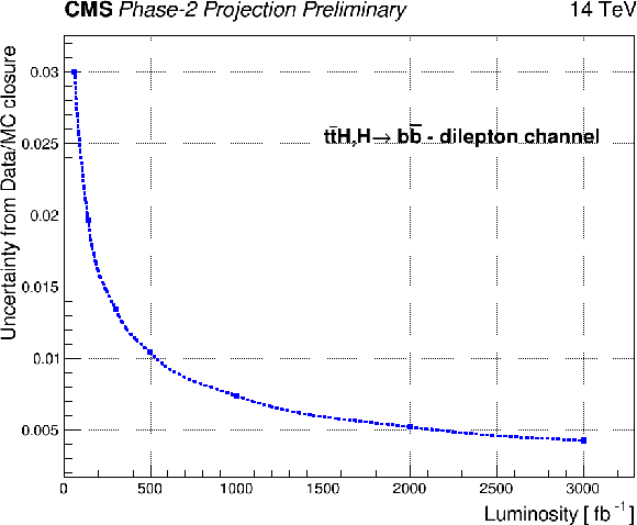
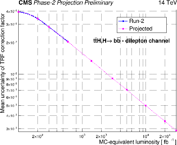
png pdf	Figure 6: Left: Projected background rate uncertainty originating from the data to simulation compatibility of the TRF prediction normalization in the 3b VR as a function of the integrated luminosity. Right: Projection of the uncertainty originating from the background prediction correction factor. The graph shows the average per- ${m_{\mathrm{b\bar{b}}}}$ -bin value of the 68% confidence interval of the 1$^{st}$ degree polynomial which is used to correct the background prediction as a function of the simulated luminosity.
png	Figure 6-a: Left: Projected background rate uncertainty originating from the data to simulation compatibility of the TRF prediction normalization in the 3b VR as a function of the integrated luminosity. Right: Projection of the uncertainty originating from the background prediction correction factor. The graph shows the average per- ${m_{\mathrm{b\bar{b}}}}$ -bin value of the 68% confidence interval of the 1$^{st}$ degree polynomial which is used to correct the background prediction as a function of the simulated luminosity.
png	Figure 6-b: Left: Projected background rate uncertainty originating from the data to simulation compatibility of the TRF prediction normalization in the 3b VR as a function of the integrated luminosity. Right: Projection of the uncertainty originating from the background prediction correction factor. The graph shows the average per- ${m_{\mathrm{b\bar{b}}}}$ -bin value of the 68% confidence interval of the 1$^{st}$ degree polynomial which is used to correct the background prediction as a function of the simulated luminosity.
png pdf	Figure 7: Projected estimated significance shown as a function of the integrated luminosity for the statistical uncertainties only scenario (black), the Run 2 uncertainty scenario (magenta), the conservative scenario (light blue) and the realistic scenario (green).
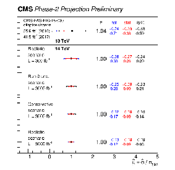
png pdf	Figure 8: Best fit values of the signal strength modifiers $\mu $ obtained in the latest CMS published result [4] (top) and for the fit of the Asimov dataset constructed for 3000 fb$^{-1}$ for the different uncertainty scenarios. Also shown are the 68% expected confidence intervals (blue error bar) which are additionally split into their statistical (red error bar) and systematic (black error bar) components.

Tables
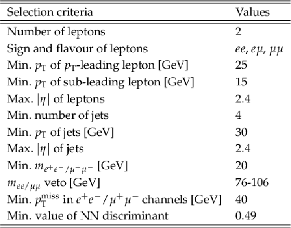
png pdf	Table 1: Baseline event selection criteria.
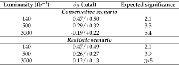
png pdf	Table 2: Expected significance and total (statistical and systematic) uncertainty on the signal strength modifier ($\delta \mu $) calculated for different values of integrated luminosity for the conservative and the most realistic uncertainty extrapolation scenarios.

Summary

The discovery of the Higgs boson has played a key role in understanding the SM. With increased integrated luminosity acquired, the LHC has opened a new era of precision measurements allowing us to study the properties of this important particle, thoroughly testing the consistency of the foundations of the SM. The HL-LHC will provide a unique opportunity to extensively test the Higgs boson properties with increased statistical precision. For the prospective studies presented in this summary, a novel alternative approach with respect to the one presented in Ref. [4] was considered. The novel approach introduced is able to overcome the hurdle of being systematic-uncertainty-limited since the main background, arising from $\mathrm{t\bar{t}} $+jets events, is predicted with a data-based method. It also provides a measurement utilizing the mass of the Higgs boson as an observable, hence being orthogonal and complementary to the approaches which utilize the output of a ML estimator. Different uncertainty extrapolation scenarios were studied to take into account the different running conditions and expected increase in luminosity. With this analysis approach, one should be able to reach discovery with the dilepton channel alone accompanied by a significantly improved precision with as much as 1/3 of the HL-LHC integrated luminosity. A measurement that will utilize the full HL-LHC integrated luminosity can result to approximately 13% total uncertainty on the signal cross section. This translates to a similar level of precision in measuring $y_{t}$ and will allow us to probe possible deviations from the SM expectation.

References
1	C. Englert et al.	Precision measurements of higgs couplings: implications for new physics scales	Journal of Physics G: Nuclear and Particle Physics 41 (Sep, 2014) 113001
2	ATLAS Collaboration	Observation of Higgs boson production in association with a top quark pair at the LHC with the ATLAS detector	PLB 784 (2018) 159	1806.00425
3	CMS Collaboration	Observation of $ \mathrm{t\overline{t}} $H production	PRL 120 (2018) 231801	CMS-HIG-17-035 1804.02610
4	CMS Collaboration	Measurement of $ \mathrm{t\overline{t}H} $ production in the $ \mathrm{H\rightarrow b\overline{b}} $ decay channel in $ 41.5 \mathrm{fb}^{-1} $ of proton-proton collision data at $ \sqrt{s}=13 \mathrm{TeV} $	CMS-PAS-HIG-18-030	CMS-PAS-HIG-18-030
5	CMS Collaboration	Search for $ \mathrm{t}\overline{\mathrm{t}}\mathrm{H} $ production in the $ \mathrm{H}\to \mathrm{b}\overline{\mathrm{b}} $ decay channel with leptonic $ \mathrm{t}\overline{\mathrm{t}} $ decays in proton-proton collisions at $ \sqrt{s}= $ 13 TeV	JHEP 03 (2019) 026	CMS-HIG-17-026 1804.03682
6	ATLAS Collaboration	Measurement of Higgs boson decay into $ b $-quarks in associated production with a top-quark pair in $ pp $ collisions at $ \sqrt{s}= $ 13 TeV with the ATLAS detector	11, 2021. Submitted to JHEP	2111.06712
7	LHC Higgs Cross Section Working Group Collaboration	Handbook of LHC Higgs Cross Sections: 4. Deciphering the Nature of the Higgs Sector		1610.07922
8	G. Anagnostou	Searching in 2-dimensional mass space for final states with 2 invisible particles	Journal of High Energy Physics 2021 (Jul, 2021)
9	G. Anagnostou	Model Independent Search in 2-Dimensional Mass Space	ArXiv e-prints (December, 2011)	1112.3379
10	ATLAS Collaboration	Search for the standard model higgs boson decaying into $ {\rm b\bar{b}} $ produced in association with top quarks decaying hadronically in pp collisions at $ \sqrt{s}=8 \mathrm{TeV} $ with the $ \mathrm{ATLAS} $ detector	Journal of High Energy Physics 2016 (May, 2016)
11	ATLAS and CMS Collaborations	Report from Working Group 2: Higgs Physics at the HL-LHC and HE-LHC	CERN Yellow Rep. Monogr. 7 (2019) 221--584	1902.00134
12	M. Czakon and A. Mitov	Top++: A program for the calculation of the top-pair cross-section at hadron colliders	Computer Physics Communications 185 (2014), no. 11, 2930--2938
13	CMS Collaboration	Technical Proposal for the Phase-II Upgrade of the CMS Detector	CMS-PAS-TDR-15-002	CMS-PAS-TDR-15-002
14	CMS Collaboration	The Phase-2 Upgrade of the CMS Tracker	CMS-PAS-TDR-17-001	CMS-PAS-TDR-17-001
15	CMS Collaboration	The Phase-2 Upgrade of the CMS Endcap Calorimeter	CMS-PAS-TDR-17-007	CMS-PAS-TDR-17-007
16	CMS Collaboration	The Phase-2 Upgrade of the CMS Muon Detectors	CMS-PAS-TDR-17-003	CMS-PAS-TDR-17-003
17	CMS Collaboration	A MIP Timing Detector for the CMS Phase-2 Upgrade	CMS-PAS-TDR-19-002	CMS-PAS-TDR-19-002
18	DELPHES 3 Collaboration	DELPHES 3, A modular framework for fast simulation of a generic collider experiment	JHEP 02 (2014) 057	1307.6346
19	GEANT4 Collaboration	GEANT4--a simulation toolkit	NIMA 506 (2003) 250--303
20	P. Nason	A New method for combining NLO QCD with shower Monte Carlo algorithms	JHEP 11 (2004) 040	hep-ph/0409146
21	S. Frixione, P. Nason, and C. Oleari	Matching NLO QCD computations with Parton Shower simulations: the POWHEG method	JHEP 11 (2007) 070	0709.2092
22	S. Alioli, P. Nason, C. Oleari, and E. Re	A general framework for implementing NLO calculations in shower Monte Carlo programs: the POWHEG BOX	JHEP 06 (2010) 043	1002.2581
23	H. B. Hartanto, B. Jager, L. Reina, and D. Wackeroth	Higgs boson production in association with top quarks in the POWHEG BOX	PRD 91 (2015), no. 9, 094003	1501.04498
24	T. Je\vzo and P. Nason	On the Treatment of Resonances in Next-to-Leading Order Calculations Matched to a Parton Shower	JHEP 12 (2015) 065	1509.09071
25	NNPDF Collaboration	Parton distributions from high-precision collider data	EPJC 77 (2017), no. 10, 663	1706.00428
26	T. Sjostrand et al.	An introduction to PYTHIA 8.2	CPC 191 (2015) 159--177	1410.3012
27	CMS Collaboration	Extraction and validation of a new set of CMS PYTHIA8 tunes from underlying-event measurements	EPJC 80 (2020), no. 1, 4	CMS-GEN-17-001 1903.12179
28	M. Czakon and A. Mitov	Top++: A Program for the Calculation of the Top-Pair Cross-Section at Hadron Colliders	CPC 185 (2014) 2930	1112.5675
29	M. Cacciari et al.	Top-pair production at hadron colliders with next-to-next-to-leading logarithmic soft-gluon resummation	PLB 710 (2012) 612--622	1111.5869
30	CMS Collaboration	Particle-flow reconstruction and global event description with the CMS detector	JINST 12 (2017) P10003	CMS-PRF-14-001 1706.04965
31	CMS Collaboration	Description and performance of track and primary-vertex reconstruction with the CMS tracker	JINST 9 (2014) P10009	CMS-TRK-11-001 1405.6569
32	CMS Collaboration	Performance of missing transverse momentum reconstruction in proton-proton collisions at $ \sqrt{s} = $ 13 TeV using the CMS detector	JINST 14 (2019), no. 07, P07004	CMS-JME-17-001 1903.06078
33	M. Cacciari, G. P. Salam, and G. Soyez	The anti-$ k_t $ jet clustering algorithm	JHEP 04 (2008) 063	0802.1189
34	M. Cacciari, G. P. Salam, and G. Soyez	The Catchment Area of Jets	JHEP 04 (2008) 005	0802.1188
35	CMS Collaboration	B-tagging performance of the $ \mathrm{CMS} \mathrm{L} $egacy dataset 2018.	CDS
36	CMS Collaboration	The Phase-2 Upgrade of the CMS Data Acquisition and High Level Trigger	CDS
37	F. Chollet et al.
38	L. Sonnenschein	Analytical solution of tt dilepton equations	73 (March, 2006) 054015	hep-ph/0603011
39	NNPDF Collaboration	Parton distributions for the LHC Run II	JHEP 04 (2015) 040	1410.8849
40	A. Buckley et al.	LHAPDF6: parton density access in the LHC precision era	EPJC 75 (2015) 132	1412.7420
41	CMS Collaboration	CMS luminosity measurement for the 2017 data-taking period at $ \sqrt{s} = $ 13 TeV	CDS
42	ATLAS Collaboration	Measurement of the Inelastic Proton-Proton Cross Section at $ \sqrt{s} = $ 13 TeV with the ATLAS Detector at the LHC	PRL 117 (2016), no. 18, 182002	1606.02625
43	R. J. Barlow and C. Beeston	Fitting using finite Monte Carlo samples	CPC 77 (1993) 219
44	ATLAS and CMS Collaborations	Addendum to the report on the physics at the HL-LHC, and perspectives for the HE-LHC: Collection of notes from ATLAS and CMS	CERN Yellow Rep. Monogr. 7 (2019) Addendum	1902.10229
45	CMS Collaboration	Sensitivity projections for Higgs boson properties measurements at the HL-LHC	CMS-PAS-FTR-18-011	CMS-PAS-FTR-18-011