CMS-PAS-BPH-16-003

CMS-PAS-BPH-16-003
Observation of the $\mathrm{B}^{*}_{\mathrm{s}2}(5840)^0\rightarrow\mathrm{B}^0\mathrm{K}^0_{\mathrm{S}}$ decay and studies of excited $\mathrm{B}^0_\mathrm{s}$ mesons in proton-proton collisions at $\sqrt{s}=$ 8 TeV
CMS Collaboration
June 2018

Abstract: The observation of the $\mathrm{B}^{}_{\mathrm{s}2}(5840)^0\rightarrow\mathrm{B}^0\mathrm{K}^0_{\mathrm{S}}$ decay is presented and a measurement of its relative branching fraction to the $\mathrm{B}^{}_{\mathrm{s}2}(5840)^0\rightarrow\mathrm{B}^+\mathrm{K}^{-}$ decay using a data sample of 19.6 fb $^{-1}$ collected with the CMS detector in proton-proton collision at the centre-of-mass energy 8 TeV. The analysis is performed by studying P-wave $\mathrm{B}^{0}_\mathrm{s}$ meson decays into $\mathrm{B}^+\mathrm{K}^-$ and $\mathrm{B}^0 \mathrm{K}^0_{\mathrm{S}}$ states, where the ground-state $\mathrm{B}$ mesons are identified using the decays $\mathrm{B}^+ \rightarrow \mathrm{J}/\psi\mathrm{K}^+$ and $\mathrm{B}^0 \rightarrow \mathrm{J}/\psi\mathrm{K}^+ \pi^-$ . The masses of P-wave $\mathrm{B}^0_\mathrm{s}$ meson states are measured and the natural width of the $\mathrm{B}^{}_{\mathrm{s}2}(5840)^0$ state is determined to be $\Gamma(\mathrm{B}^{}_{\mathrm{s}2}(5840)^0)=$ (1.52 $\pm$ 0.34 (stat) $\pm$ 0.30 (syst) MeV. The first measurement of the mass difference between the charged and neutral $\mathrm{B}^*$ mesons is also presented.
Links: CDS record (PDF) ; inSPIRE record ; CADI line (restricted) ; These preliminary results are superseded in this paper, EPJC 78 (2018) 939. The superseded preliminary plots can be found here.

Figures & Tables	Summary	References	CMS Publications

Figures
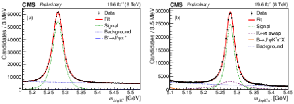
png pdf	Figure 1: Invariant mass distributions of ${\mathrm {J} / \psi} {{{\mathrm {K}}} ^+}$ (a) and ${\mathrm {J} / \psi} {{{\mathrm {K}}} ^+} {{\pi} ^-}$ (b) candidates in the data with the fit results superimposed.
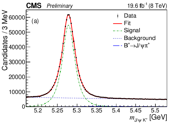
png pdf	Figure 1-a: Invariant mass distributions of ${\mathrm {J} / \psi} {{{\mathrm {K}}} ^+}$ (a) and ${\mathrm {J} / \psi} {{{\mathrm {K}}} ^+} {{\pi} ^-}$ (b) candidates in the data with the fit results superimposed.
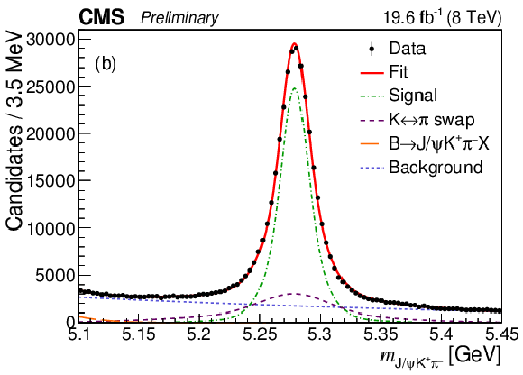
png pdf	Figure 1-b: Invariant mass distributions of ${\mathrm {J} / \psi} {{{\mathrm {K}}} ^+}$ (a) and ${\mathrm {J} / \psi} {{{\mathrm {K}}} ^+} {{\pi} ^-}$ (b) candidates in the data with the fit results superimposed.
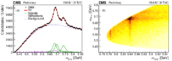
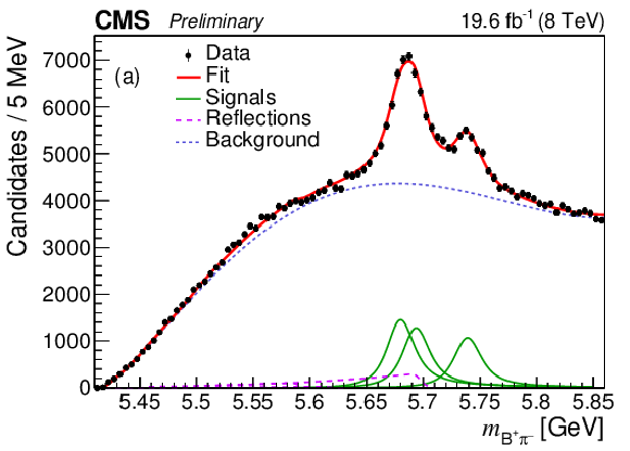
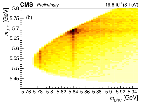
png pdf	Figure 2: (a) The fitted ${{{\mathrm {B}} ^+} {{\pi} ^-}}$ invariant mass distribution. The points represent the data, the thick solid curve is the fit projection, the thin lines indicate the excited ${{\mathrm {B}} ^0}$ signal contributions, the dashed curve is the background, and the long-dashed lines show the contributions from the excited ${{\mathrm {B}} ^0_ {\mathrm {s}}}$ decays. (b) Two-dimensional distribution of ${m_{{{{\mathrm {B}} ^+}} {{{\mathrm {K}}} ^-}}}$ versus ${m_{{{{\mathrm {B}} ^+}} {{\pi} ^-}}}$ in data.
png pdf	Figure 2-a: (a) The fitted ${{{\mathrm {B}} ^+} {{\pi} ^-}}$ invariant mass distribution. The points represent the data, the thick solid curve is the fit projection, the thin lines indicate the excited ${{\mathrm {B}} ^0}$ signal contributions, the dashed curve is the background, and the long-dashed lines show the contributions from the excited ${{\mathrm {B}} ^0_ {\mathrm {s}}}$ decays. (b) Two-dimensional distribution of ${m_{{{{\mathrm {B}} ^+}} {{{\mathrm {K}}} ^-}}}$ versus ${m_{{{{\mathrm {B}} ^+}} {{\pi} ^-}}}$ in data.
png pdf	Figure 2-b: (a) The fitted ${{{\mathrm {B}} ^+} {{\pi} ^-}}$ invariant mass distribution. The points represent the data, the thick solid curve is the fit projection, the thin lines indicate the excited ${{\mathrm {B}} ^0}$ signal contributions, the dashed curve is the background, and the long-dashed lines show the contributions from the excited ${{\mathrm {B}} ^0_ {\mathrm {s}}}$ decays. (b) Two-dimensional distribution of ${m_{{{{\mathrm {B}} ^+}} {{{\mathrm {K}}} ^-}}}$ versus ${m_{{{{\mathrm {B}} ^+}} {{\pi} ^-}}}$ in data.
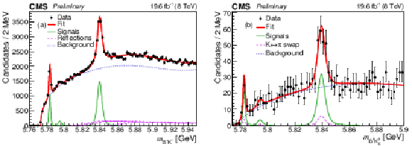
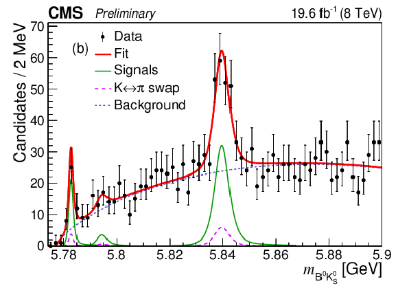
png pdf	Figure 3: Invariant mass distributions of ${{{\mathrm {B}} ^+} {{{\mathrm {K}}} ^-}}$ (a) and ${{{\mathrm {B}} ^0} {{{\mathrm {K}}} ^0_{\rm {S}}}}$ (b) candidates with the results of the fit overlaid. The points represent the data, the thick curves are the fit projections, the thin lines display the signal contributions, and the long-dashed lines show: in (a) the contributions from excited ${{\mathrm {B}} ^0}$ meson decays; in (b) the contributions from ${{{\mathrm {K}}} ^\pm} \leftrightarrow {{\pi} ^\pm}$ swap in ${{\mathrm {B}} ^0}$ reconstruction. The dashed lines show the background contribution.
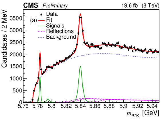
png pdf	Figure 3-a: Invariant mass distributions of ${{{\mathrm {B}} ^+} {{{\mathrm {K}}} ^-}}$ (a) and ${{{\mathrm {B}} ^0} {{{\mathrm {K}}} ^0_{\rm {S}}}}$ (b) candidates with the results of the fit overlaid. The points represent the data, the thick curves are the fit projections, the thin lines display the signal contributions, and the long-dashed lines show: in (a) the contributions from excited ${{\mathrm {B}} ^0}$ meson decays; in (b) the contributions from ${{{\mathrm {K}}} ^\pm} \leftrightarrow {{\pi} ^\pm}$ swap in ${{\mathrm {B}} ^0}$ reconstruction. The dashed lines show the background contribution.
png pdf	Figure 3-b: Invariant mass distributions of ${{{\mathrm {B}} ^+} {{{\mathrm {K}}} ^-}}$ (a) and ${{{\mathrm {B}} ^0} {{{\mathrm {K}}} ^0_{\rm {S}}}}$ (b) candidates with the results of the fit overlaid. The points represent the data, the thick curves are the fit projections, the thin lines display the signal contributions, and the long-dashed lines show: in (a) the contributions from excited ${{\mathrm {B}} ^0}$ meson decays; in (b) the contributions from ${{{\mathrm {K}}} ^\pm} \leftrightarrow {{\pi} ^\pm}$ swap in ${{\mathrm {B}} ^0}$ reconstruction. The dashed lines show the background contribution.
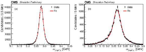
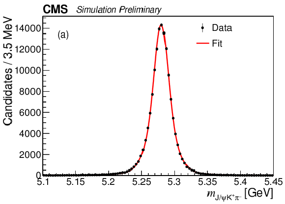
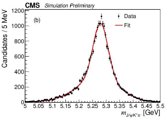
png pdf	Figure 4: ${m_{{{\mathrm {B}} ^0}}}$ distribution in simulation with the fit result superimposed. (a) signal with matching; (b) reflection from ' ${{{\mathrm {K}}} ^\pm} \leftrightarrow {{\pi} ^\pm}$ swap' obtained by requiring the reconstructed kaon candidate to be matched to the generated pion and vice versa.
png pdf	Figure 4-a: ${m_{{{\mathrm {B}} ^0}}}$ distribution in simulation with the fit result superimposed. (a) signal with matching; (b) reflection from ' ${{{\mathrm {K}}} ^\pm} \leftrightarrow {{\pi} ^\pm}$ swap' obtained by requiring the reconstructed kaon candidate to be matched to the generated pion and vice versa.
png pdf	Figure 4-b: ${m_{{{\mathrm {B}} ^0}}}$ distribution in simulation with the fit result superimposed. (a) signal with matching; (b) reflection from ' ${{{\mathrm {K}}} ^\pm} \leftrightarrow {{\pi} ^\pm}$ swap' obtained by requiring the reconstructed kaon candidate to be matched to the generated pion and vice versa.
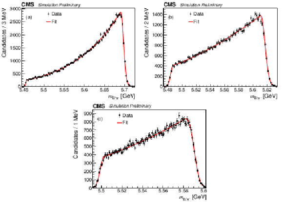
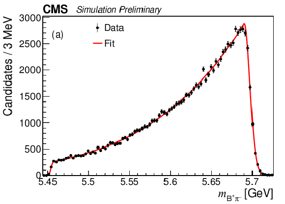
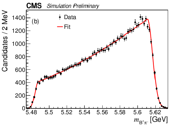
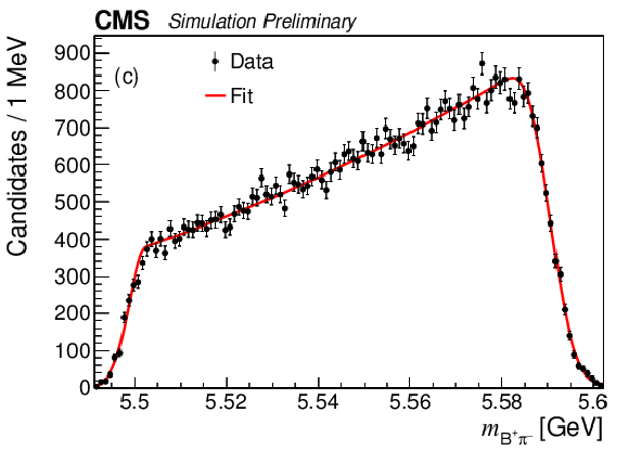
png pdf	Figure 5: The ${{{\mathrm {B}} ^+} {{\pi} ^-}}$ invariant mass distributions from the simulated decay: (a) ${{{\mathrm {B}} ^{}_{{\mathrm {s}} 2}} \to {{\mathrm {B}} ^+} {{{\mathrm {K}}} ^-}}$ ; (b) ${{{\mathrm {B}} ^{}_{{\mathrm {s}} 2}} \to {{\mathrm {B}} ^{+}} {{{\mathrm {K}}} ^-}}$ ; (c) ${{\mathrm {B}} _{{\mathrm {s}} 1}} \to {{\mathrm {B}} ^{+}} {{{\mathrm {K}}} ^-}$ .
png pdf	Figure 5-a: The ${{{\mathrm {B}} ^+} {{\pi} ^-}}$ invariant mass distributions from the simulated decay: (a) ${{{\mathrm {B}} ^{}_{{\mathrm {s}} 2}} \to {{\mathrm {B}} ^+} {{{\mathrm {K}}} ^-}}$ ; (b) ${{{\mathrm {B}} ^{}_{{\mathrm {s}} 2}} \to {{\mathrm {B}} ^{+}} {{{\mathrm {K}}} ^-}}$ ; (c) ${{\mathrm {B}} _{{\mathrm {s}} 1}} \to {{\mathrm {B}} ^{+}} {{{\mathrm {K}}} ^-}$ .
png pdf	Figure 5-b: The ${{{\mathrm {B}} ^+} {{\pi} ^-}}$ invariant mass distributions from the simulated decay: (a) ${{{\mathrm {B}} ^{}_{{\mathrm {s}} 2}} \to {{\mathrm {B}} ^+} {{{\mathrm {K}}} ^-}}$ ; (b) ${{{\mathrm {B}} ^{}_{{\mathrm {s}} 2}} \to {{\mathrm {B}} ^{+}} {{{\mathrm {K}}} ^-}}$ ; (c) ${{\mathrm {B}} _{{\mathrm {s}} 1}} \to {{\mathrm {B}} ^{+}} {{{\mathrm {K}}} ^-}$ .
png pdf	Figure 5-c: The ${{{\mathrm {B}} ^+} {{\pi} ^-}}$ invariant mass distributions from the simulated decay: (a) ${{{\mathrm {B}} ^{}_{{\mathrm {s}} 2}} \to {{\mathrm {B}} ^+} {{{\mathrm {K}}} ^-}}$ ; (b) ${{{\mathrm {B}} ^{}_{{\mathrm {s}} 2}} \to {{\mathrm {B}} ^{+}} {{{\mathrm {K}}} ^-}}$ ; (c) ${{\mathrm {B}} _{{\mathrm {s}} 1}} \to {{\mathrm {B}} ^{+}} {{{\mathrm {K}}} ^-}$ .
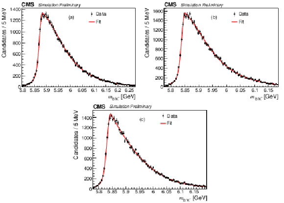
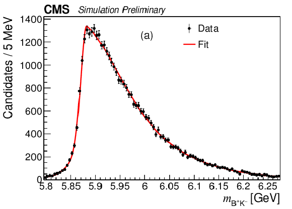
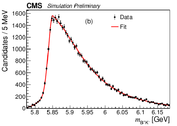
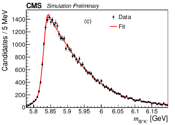
png pdf	Figure 6: The ${{{\mathrm {B}} ^+} {{{\mathrm {K}}} ^-}}$ invariant mass distributions from the simulated decay: (a) ${{\mathrm {B}} ^{}_{2}} \to {{\mathrm {B}} ^+} {{\pi} ^-}$ , (b) ${{\mathrm {B}} ^{}_{2}} \to {{\mathrm {B}} ^{+}} {{\pi} ^-}$ and (c) ${{\mathrm {B}} _{1}} \to {{\mathrm {B}} ^{+}} {{\pi} ^-}$ .
png pdf	Figure 6-a: The ${{{\mathrm {B}} ^+} {{{\mathrm {K}}} ^-}}$ invariant mass distributions from the simulated decay: (a) ${{\mathrm {B}} ^{}_{2}} \to {{\mathrm {B}} ^+} {{\pi} ^-}$ , (b) ${{\mathrm {B}} ^{}_{2}} \to {{\mathrm {B}} ^{+}} {{\pi} ^-}$ and (c) ${{\mathrm {B}} _{1}} \to {{\mathrm {B}} ^{+}} {{\pi} ^-}$ .
png pdf	Figure 6-b: The ${{{\mathrm {B}} ^+} {{{\mathrm {K}}} ^-}}$ invariant mass distributions from the simulated decay: (a) ${{\mathrm {B}} ^{}_{2}} \to {{\mathrm {B}} ^+} {{\pi} ^-}$ , (b) ${{\mathrm {B}} ^{}_{2}} \to {{\mathrm {B}} ^{+}} {{\pi} ^-}$ and (c) ${{\mathrm {B}} _{1}} \to {{\mathrm {B}} ^{+}} {{\pi} ^-}$ .
png pdf	Figure 6-c: The ${{{\mathrm {B}} ^+} {{{\mathrm {K}}} ^-}}$ invariant mass distributions from the simulated decay: (a) ${{\mathrm {B}} ^{}_{2}} \to {{\mathrm {B}} ^+} {{\pi} ^-}$ , (b) ${{\mathrm {B}} ^{}_{2}} \to {{\mathrm {B}} ^{+}} {{\pi} ^-}$ and (c) ${{\mathrm {B}} _{1}} \to {{\mathrm {B}} ^{+}} {{\pi} ^-}$ .

Tables
png pdf	Table 1: Results on ${{\mathrm {B}} ^{()}_{{\mathrm {s}} 1,2}}$ from previous measurements. Mass differences are designated as ${\Delta M_{{{\mathrm {B}} _{{\mathrm {s}} 1}}}^{\pm}} \equiv {M({{\mathrm {B}} _{{\mathrm {s}} 1}})-M({{\mathrm {B}} ^{+}})-M({{{\mathrm {K}}} ^-})}$ , ${\Delta M_{{{\mathrm {B}} ^{}_{{\mathrm {s}} 2}}}^{\pm}} \equiv {M({{\mathrm {B}} ^{}_{{\mathrm {s}} 2}})-M({{\mathrm {B}} ^+})-M({{{\mathrm {K}}} ^-})}$ .
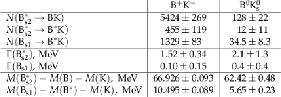
png pdf	Table 2: Results from the fits to the ${m_{{{\mathrm {B}} {{\mathrm {K}}}}}}$ distributions in data.
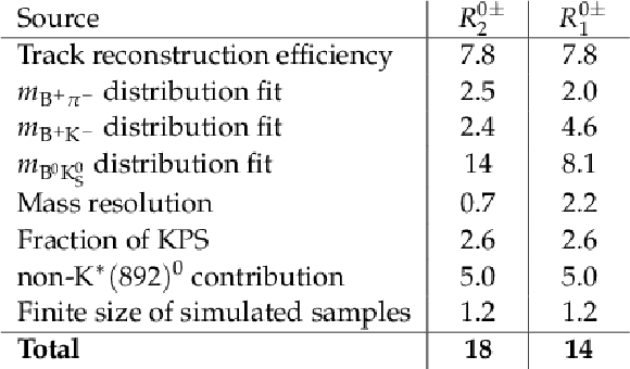
png pdf	Table 3: Systematic uncertainties in percent in the ratios ${R^{0\pm}_{2}}$ and ${R^{0\pm}_{1}}$ .
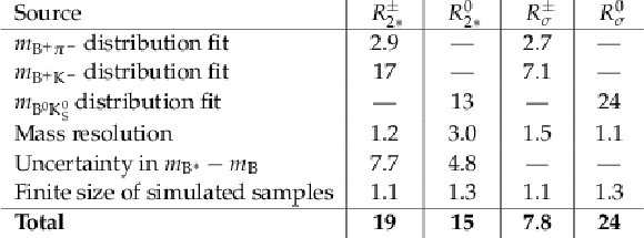
png pdf	Table 4: Systematic uncertainties (in%) in the ratios ${R^{\pm}_{2}}$ , ${R^{0}_{2}}$ , ${R^{\pm}_{\sigma}}$ , and ${R^{0}_{\sigma}}$ .
png pdf	Table 5: Systematic uncertainties (in MeV) in the measured mass differences and natural width ( ${\Gamma _{{{\mathrm {B}} ^{*}_{{\mathrm {s}} 2}}}}$ , measured only in ${{{\mathrm {B}} ^+} {{{\mathrm {K}}} ^-}}$ channel).

Summary

In summary, the P-wave

$\mathrm{B}^{0}_\mathrm{s}$ meson states are studied using a data sample corresponding to an integrated luminosity of 19.6 fb

$^{-1}$ of pp collisions collected by the CMS experiment at

$\sqrt{s} =$ 8 TeV in 2012. The observation and the first evidence are reported for the decays

$\mathrm{B}^{*}_{\mathrm{s}2}\rightarrow\mathrm{B}^0\mathrm{K}^0_{\mathrm{S}}$ and

$\mathrm{B}_{\mathrm{s}1}\rightarrow\mathrm{B}^{*0}\mathrm{K}^0_{\mathrm{S}}$ , respectively. Four ratios of branching fractions and two ratios of cross section multiplied by the branching fractions of the P-wave

$\mathrm{B}^{0}_\mathrm{s}$ mesons into B meson and kaon are measured. In addition, the differences between the

${\mathrm{B}^{(*)}_{\mathrm{s}1,2}}$ mass and the sum of B meson and kaon mass are determined, as well as the

${\mathrm{B}^{(*)}_{\mathrm{s}2}}$ natural width. Finally, using a new approach, the mass differences

$m_{\mathrm{B}^0}-m_{\mathrm{B}^+}$ and

$m_{\mathrm{B}^{*0}}-m_{\mathrm{B}^{*+}}$ are measured, where the latter mass difference is measured for the first time.

References
1	F. E. Close and Z.-p. Li	Effective heavy quark theory	PLB 289 (1992) 143	hep-ph/9206217
2	A. G. Grozin	Heavy quark effective theory	Springer Tracts Mod. Phys. 201 (2004) 1
3	CDF Collaboration	Observation of orbitally excited $\mathrm{B}_\mathrm{s}$ mesons	PRL 100 (2008) 082001	0710.4199
4	D0 Collaboration	Observation and properties of the orbitally excited B*(s2) meson	PRL 100 (2008) 082002	0711.0319
5	LHCb Collaboration	First observation of the decay $\mathrm{B}_{\rm{s2}}^(5840)^0 \to {\rm B}^{+} {\rm K}^-$ and studies of excited ${\rm B}^0_{\rm s}$ mesons	PRL 110 (2013) 151803	1211.5994
6	CDF Collaboration	Study of orbitally excited B mesons and evidence for a new $\mathrm{B}\pi$ resonance	PRD 90 (2014) 012013	1309.5961
7	CMS Collaboration	The CMS experiment at the CERN LHC	JINST 3 (2008) S08004	CMS-00-001
8	CMS Collaboration	Description and performance of track and primary-vertex reconstruction with the CMS tracker	JINST 9 (2014) P10009	CMS-TRK-11-001 1405.6569
9	CMS Collaboration	Performance of CMS muon reconstruction in $\rm{pp}$ collision events at $\sqrt{s} =$ 7 TeV	JINST 7 (2012) P10002	CMS-MUO-10-004 1206.4071
10	CMS Collaboration	The CMS trigger system	JINST 12 (2017) P01020	CMS-TRG-12-001 1609.02366
11	CMS Collaboration	Measurement of the CP-violating weak phase $\phi_s$ and the decay width difference $\Delta \Gamma_s$ using the B $_s^0 \to {\rm J}/\psi\phi$ (1020) decay channel in pp collisions at $\sqrt{s}=$ 8 ~TeV	PLB 757 (2016) 97	CMS-BPH-13-012 1507.07527
12	CMS Collaboration	Search for the X(5568) state decaying into $\mathrm{B}^{0}_{\mathrm{s}}\pi^{\pm}$ in proton-proton collisions at $\sqrt{s} =$ 8 TeV	PRL 120 (2018) 202005	CMS-BPH-16-002 1712.06144
13	Particle Data Group, C. Patrignani et al.	Review of particle physics	CPC 40 (2016) 100001
14	T. Sjostrand, S. Mrenna, and P. Skands	PYTHIA 6.4 physics and manual	JHEP 05 (2006) 026	hep-ph/0603175
15	D. J. Lange	The EvtGen particle decay simulation package	NIMA 462 (2001) 152
16	E. Barberio, B. van Eijk, and Z. W\cas	PHOTOS --- a universal Monte Carlo for QED radiative corrections in decays	CPC 66 (1991) 115
17	E. Barberio and Z. W\cas	PHOTOS -- a universal Monte Carlo for QED radiative corrections: version 2.0	CPC 79 (1994) 291
18	GEANT4 Collaboration	GEANT4---a simulation toolkit	NIMA 506 (2003) 250
19	M. Pivk and F. R. Le Diberder	${}_\mathrm{s}$ Plot: a statistical tool to unfold data distributions	NIMA 555 (2005) 356--369	physics/0402083
20	CMS Collaboration	Alignment of the CMS tracker with LHC and cosmic ray data	JINST 9 (2014) P06009	CMS-TRK-11-002 1403.2286
21	Z.-H. Wang, G.-L. Wang, H.-F. Fu, and Y. Jiang	The strong decays of orbitally excited $\mathrm{B}^{*}_{\rm sJ}$ mesons by improved Bethe-Salpeter method	PLB 706 (2012) 389	1202.1224
22	Q.-F. Lu et al.	Excited bottom and bottom-strange mesons in the quark model	PRD 94 (2016) 074012	1607.02812
23	X.-h. Zhong and Q. Zhao	Strong decays of heavy-light mesons in a chiral quark model	PRD 78 (2008) 014029	0803.2102
24	P. Colangelo, F. De Fazio, F. Giannuzzi, and S. Nicotri	New meson spectroscopy with open charm and beauty	PRD 86 (2012) 054024	1207.6940