

Compact Muon Solenoid
LHC, CERN
| CMS-PAS-TOP-15-014 | ||
| Measurement of the top quark mass in $\mathrm{t}\bar{\mathrm{t}}$ events with a $\mathrm{J}/\psi$ from pp collisions at 8 TeV | ||
| CMS Collaboration | ||
| March 2016 | ||
| Abstract: The first measurement of the top quark mass using top quark decays in the exclusive decay channel $\mathrm{t}\to(\mathrm{W}\to\ell\nu)$, $(\mathrm{b}\to\mathrm{J}/\psi+\mathrm{X}\to\mu^+\mu^-+\mathrm{X})$ is presented. Top quark pair events in proton-proton collisions recorded with the CMS detector at a center-of-mass energy of 8 TeV are selected. The dataset corresponds to an integrated luminosity of 19.7 fb$^{-1}$ and yields 666 $\mathrm{t}\bar{\mathrm{t}}$ events containing one $\mathrm{J}/\psi$ candidate in which the $\mathrm{J}/\psi$ decays into an opposite sign muon pair. The mass of the ($\mathrm{J}/\psi+\ell$) system, where $\ell$ is an electron or a muon from the W boson decay, is used to extract a top quark mass of $M_\mathrm{t} =$ 173.5 $\pm$ 3.0 (stat) $\pm$ 0.9 (syst) GeV. | ||
|
Links:
CDS record (PDF) ;
CADI line (restricted) ;
These preliminary results are superseded in this paper, JHEP 12 (2016) 123. The superseded preliminary plots can be found here. |
||
| Figures | |

png pdf |
Figure 1:
Pictorial view of an exclusive $ {\mathrm {J}/\psi }$ production in a $ \mathrm{ t \bar{t} } $ system. |
png pdf |
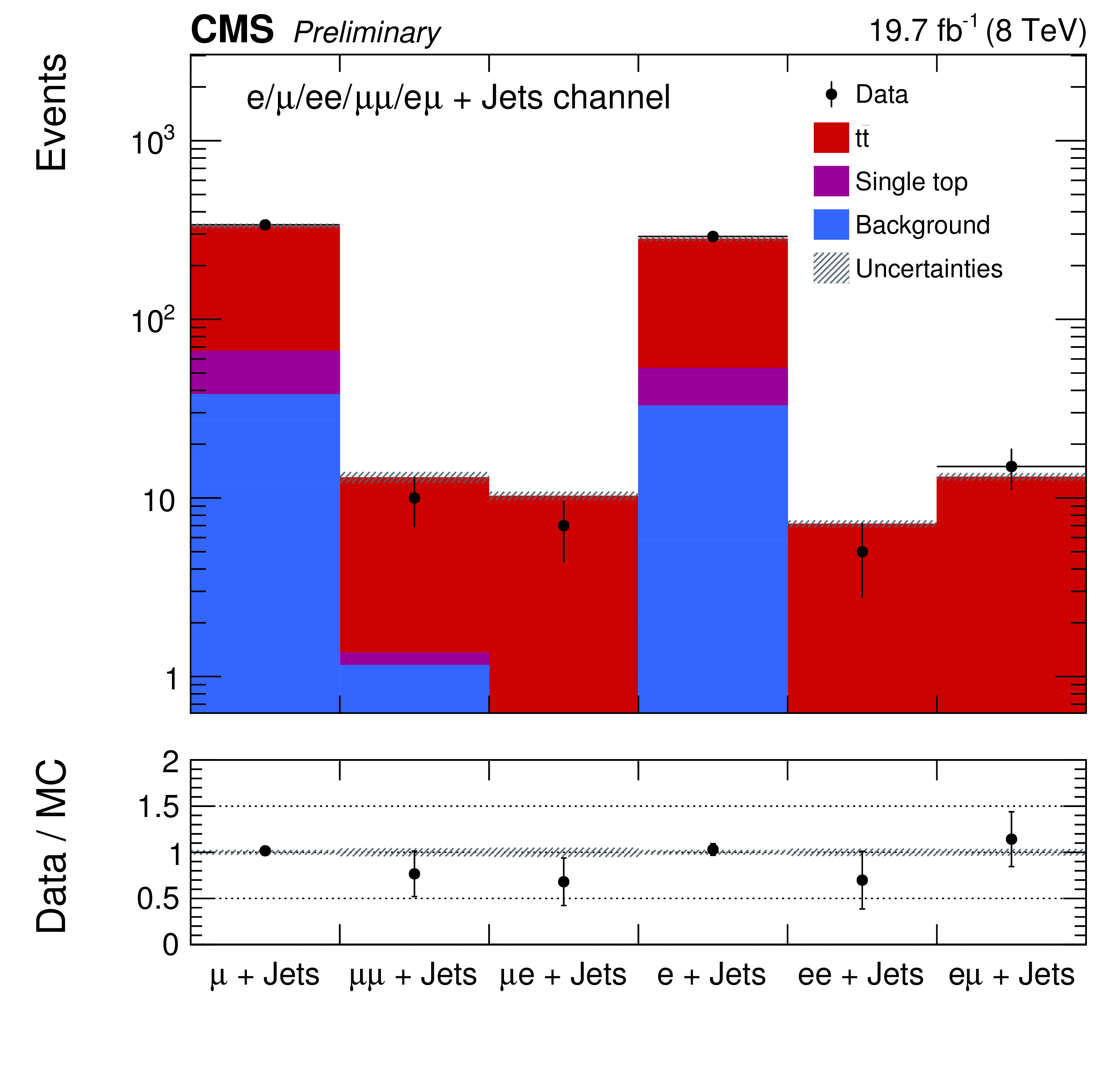
Figure 2:
Numbers of events selected in data and Monte Carlo simulations, in each channel. Processes are normalized to their theoretical cross section. The lower inset shows the ratio of the number of events observed in data over the number of events expected from simulations. |

png pdf |
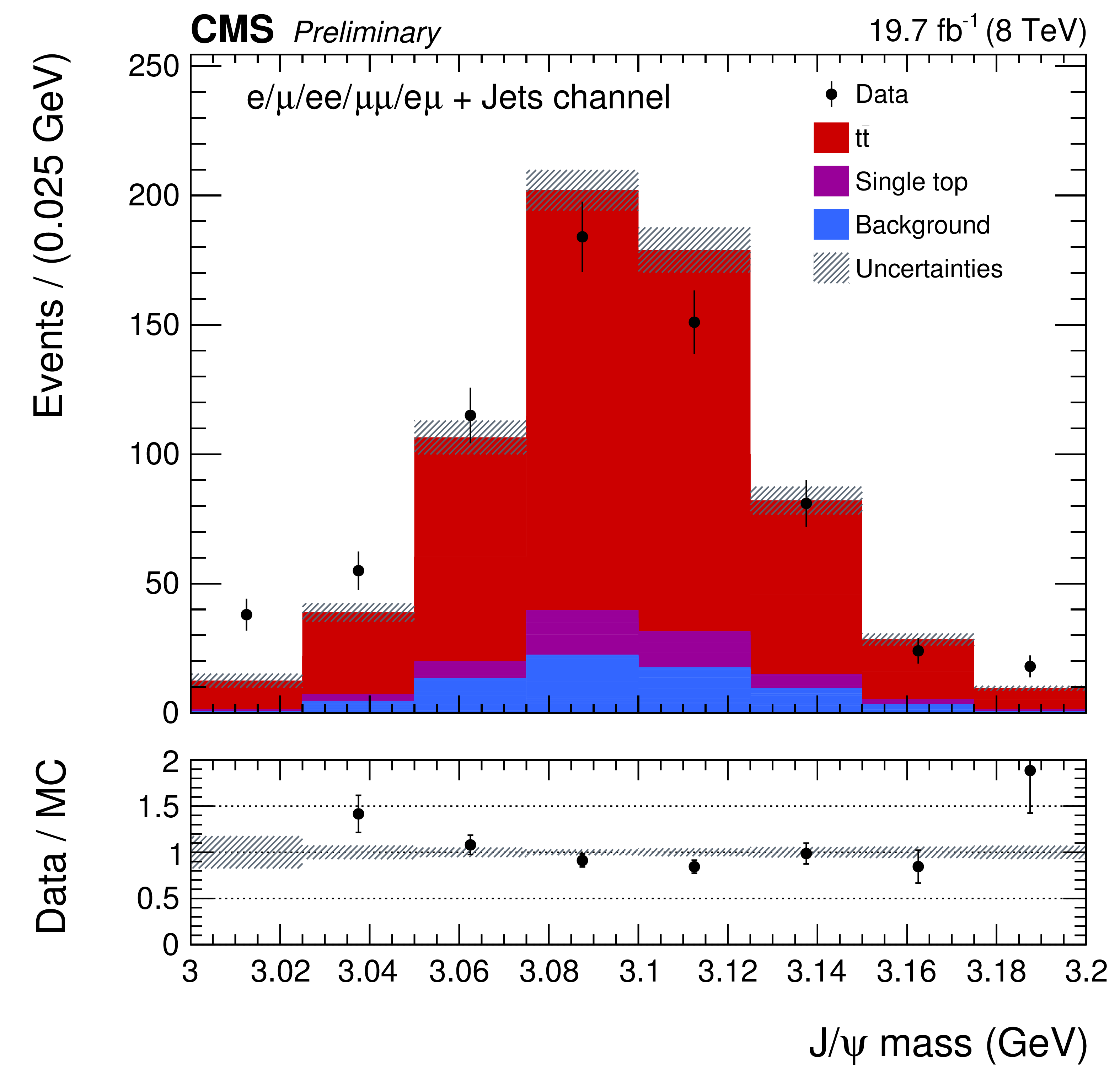
Figure 3:
Dimuon invariant mass between 2.8 and 3.4 GeV. Processes are normalized to their theoretical cross section. The lower inset shows the ratio of the number of events observed in data over the number of events expected from simulations. |

png pdf |
Figure 4-a:
Distributions of reconstructed $ {\mathrm {J}/\psi }\to \mu ^+\mu ^-$ candidate properties: transverse momentum (a), and mass(b). Processes are normalized to their theoretical cross section. The lower inset shows the ratio of the observed over the expected distributions. |
png pdf |
Figure 4-b:
Distributions of reconstructed $ {\mathrm {J}/\psi }\to \mu ^+\mu ^-$ candidate properties: transverse momentum (a), and mass(b). Processes are normalized to their theoretical cross section. The lower inset shows the ratio of the observed over the expected distributions. |

png pdf |
Figure 5-a:
Distributions of the distance in the $(\eta ,\phi )$ plane between the reconstructed $ {\mathrm {J}/\psi }$ candidate and the leading lepton (a,b), and of the invariant mass (c,d) of their combination, in the $\mu /\mu \mu /\mu \mathrm {e}+\mathrm {jets}$ channel (a,c) and in the $\mathrm {e}/\mathrm {ee}/\mathrm {e}\mu +\mathrm {jets}$ channel (b,d). Processes are normalized to their theoretical cross section. The lower inset shows the ratio of the observed over the expected distributions. |
png pdf |
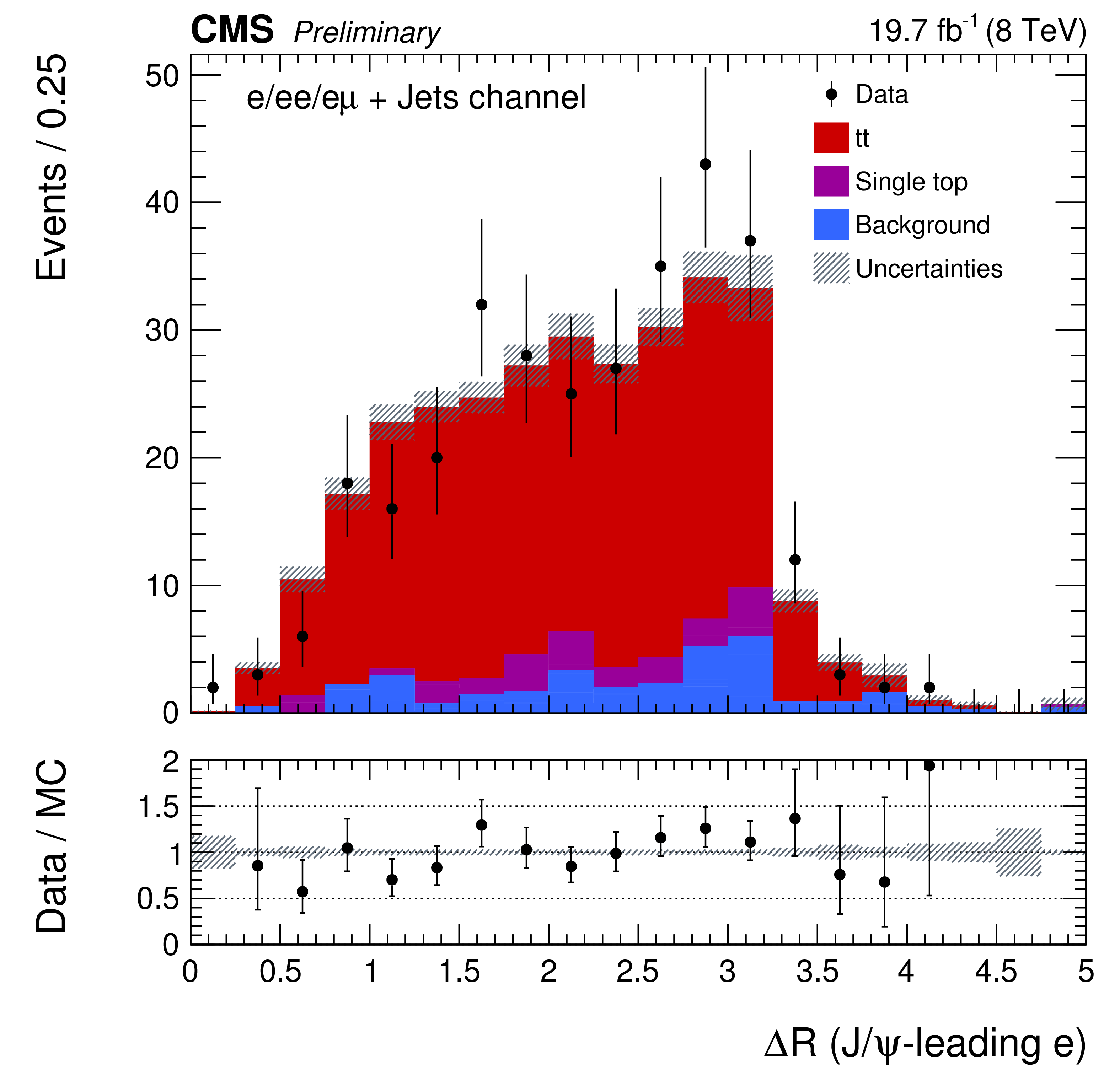
Figure 5-b:
Distributions of the distance in the $(\eta ,\phi )$ plane between the reconstructed $ {\mathrm {J}/\psi }$ candidate and the leading lepton (a,b), and of the invariant mass (c,d) of their combination, in the $\mu /\mu \mu /\mu \mathrm {e}+\mathrm {jets}$ channel (a,c) and in the $\mathrm {e}/\mathrm {ee}/\mathrm {e}\mu +\mathrm {jets}$ channel (b,d). Processes are normalized to their theoretical cross section. The lower inset shows the ratio of the observed over the expected distributions. |

png pdf |
Figure 5-c:
Distributions of the distance in the $(\eta ,\phi )$ plane between the reconstructed $ {\mathrm {J}/\psi }$ candidate and the leading lepton (a,b), and of the invariant mass (c,d) of their combination, in the $\mu /\mu \mu /\mu \mathrm {e}+\mathrm {jets}$ channel (a,c) and in the $\mathrm {e}/\mathrm {ee}/\mathrm {e}\mu +\mathrm {jets}$ channel (b,d). Processes are normalized to their theoretical cross section. The lower inset shows the ratio of the observed over the expected distributions. |
png pdf |
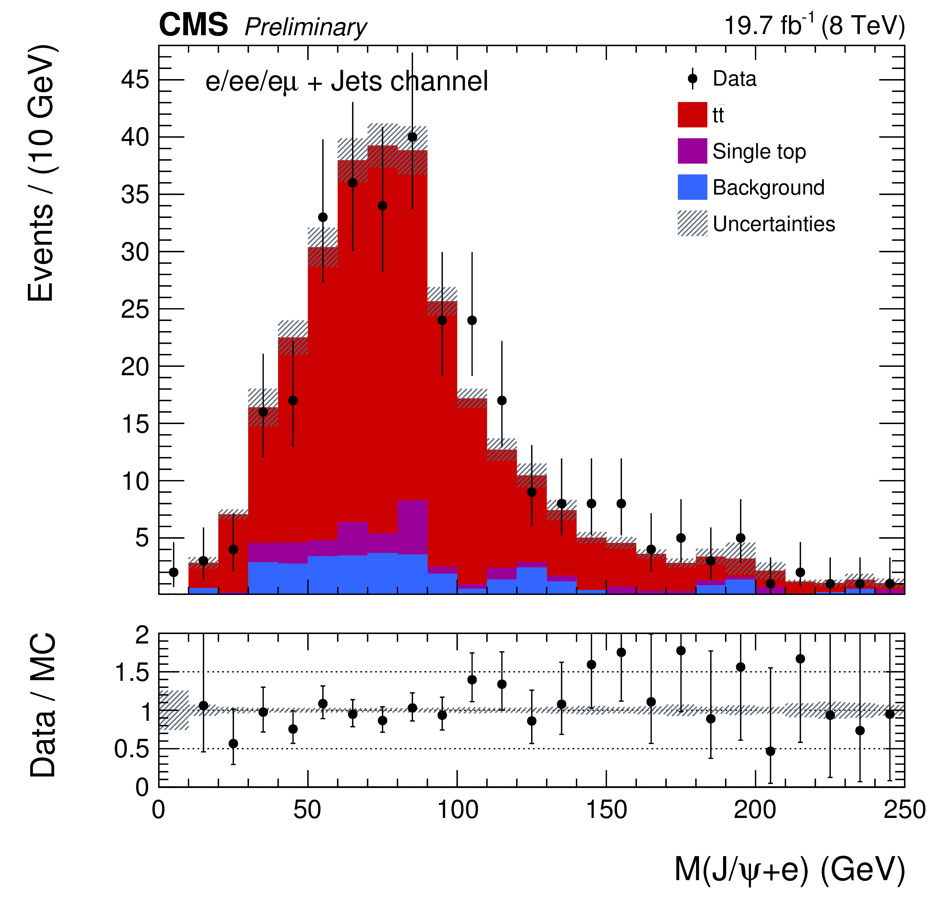
Figure 5-d:
Distributions of the distance in the $(\eta ,\phi )$ plane between the reconstructed $ {\mathrm {J}/\psi }$ candidate and the leading lepton (a,b), and of the invariant mass (c,d) of their combination, in the $\mu /\mu \mu /\mu \mathrm {e}+\mathrm {jets}$ channel (a,c) and in the $\mathrm {e}/\mathrm {ee}/\mathrm {e}\mu +\mathrm {jets}$ channel (b,d). Processes are normalized to their theoretical cross section. The lower inset shows the ratio of the observed over the expected distributions. |
png pdf |
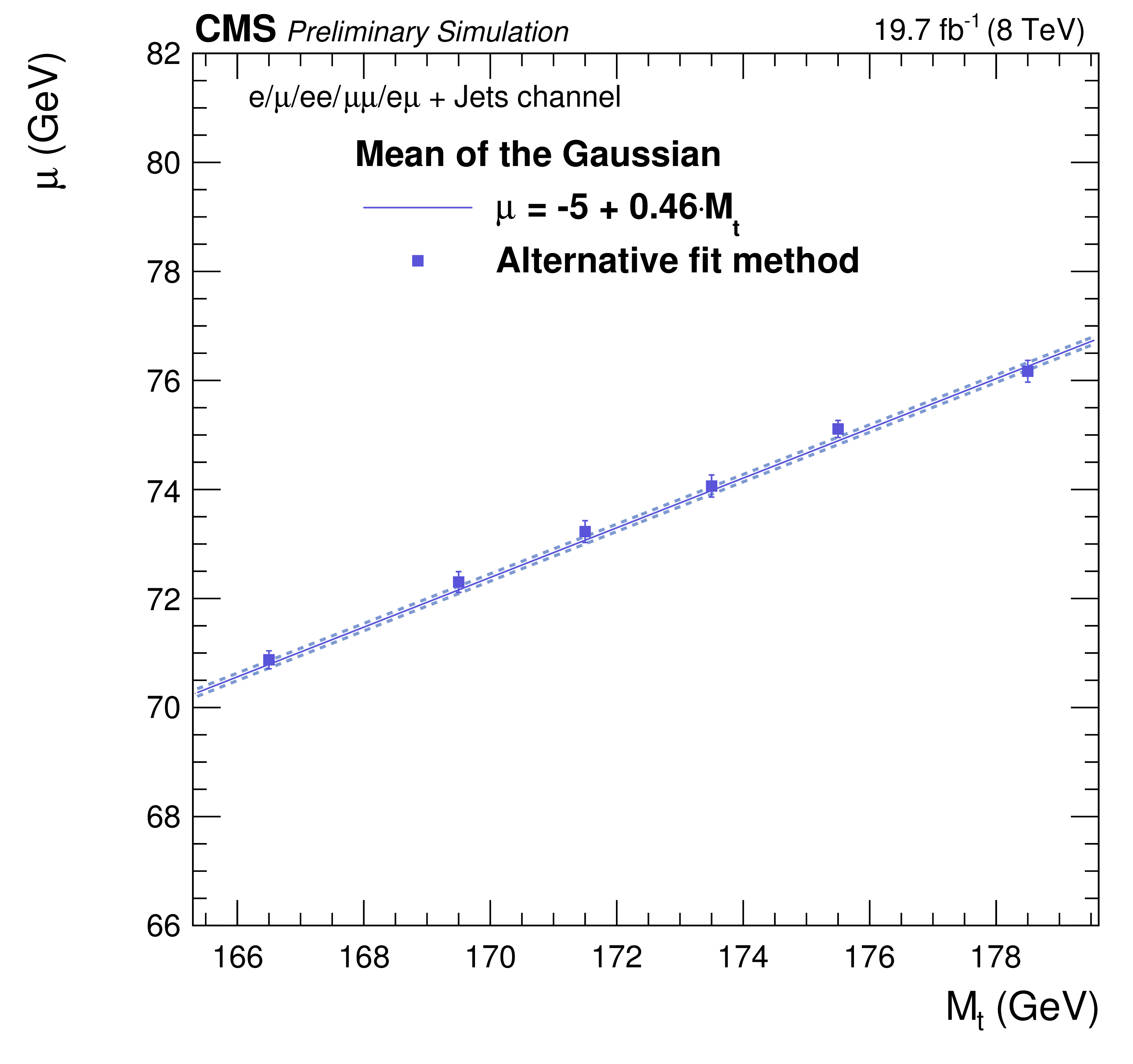
Figure 6-a:
Mean (a) and width (b) of the Gaussian function describing the peak of the $M_{ {\mathrm {J}/\psi }+\ell }$ distributions, as function of $M_\mathrm {t}$. These are the parameters with the strongest correlation to $M_\mathrm {t}$. Lines are a result of the simultaneous fit decribed in Section 4.1, while superimposed dots are a result of the alternative fit method described in Section 4.2. |

png pdf |
Figure 6-b:
Mean (a) and width (b) of the Gaussian function describing the peak of the $M_{ {\mathrm {J}/\psi }+\ell }$ distributions, as function of $M_\mathrm {t}$. These are the parameters with the strongest correlation to $M_\mathrm {t}$. Lines are a result of the simultaneous fit decribed in Section 4.1, while superimposed dots are a result of the alternative fit method described in Section 4.2. |
png pdf |
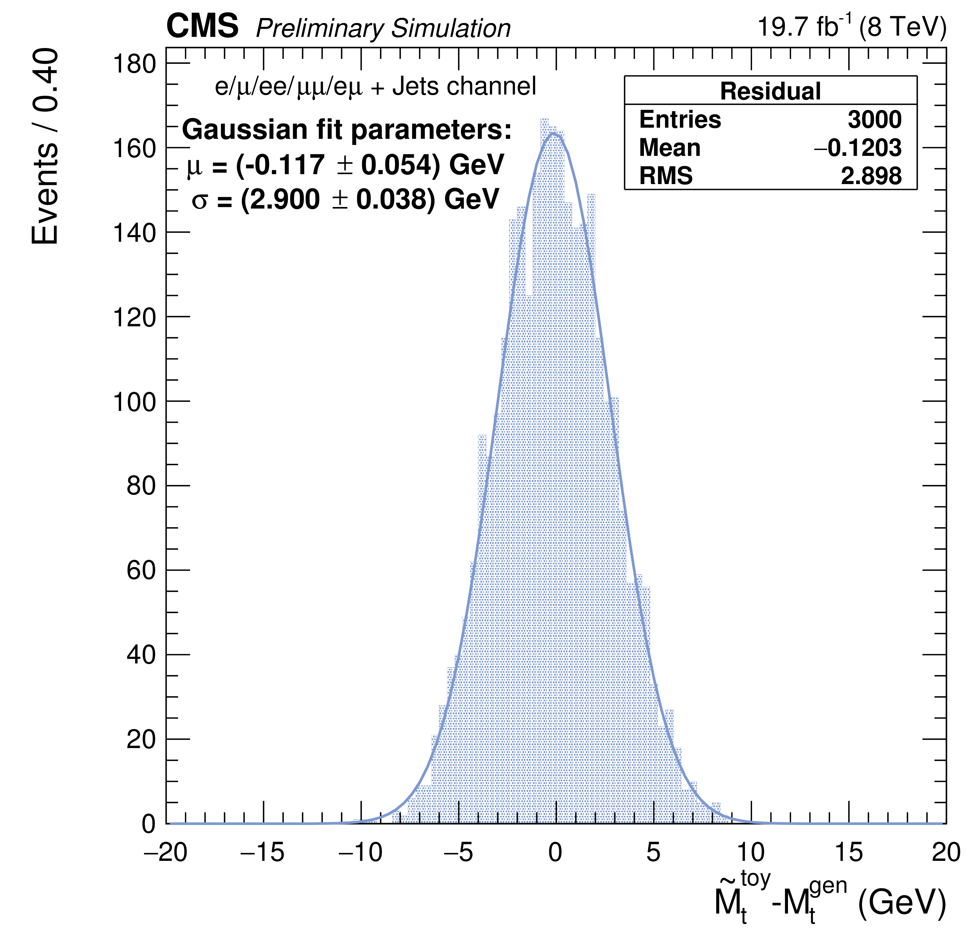
Figure 7-a:
Residual (a) and pull (b) distributions for 3 000 pseudoexperiments generated from $P_\mathrm {sig+bg}|_{M_\mathrm {t}=$ 172.5 GeV and fitted with $P_\mathrm {sig+bg}$. |

png pdf |
Figure 7-b:
Residual (a) and pull (b) distributions for 3 000 pseudoexperiments generated from $P_\mathrm {sig+bg}|_{M_\mathrm {t}=$ 172.5 GeV and fitted with $P_\mathrm {sig+bg}$. |
png pdf |
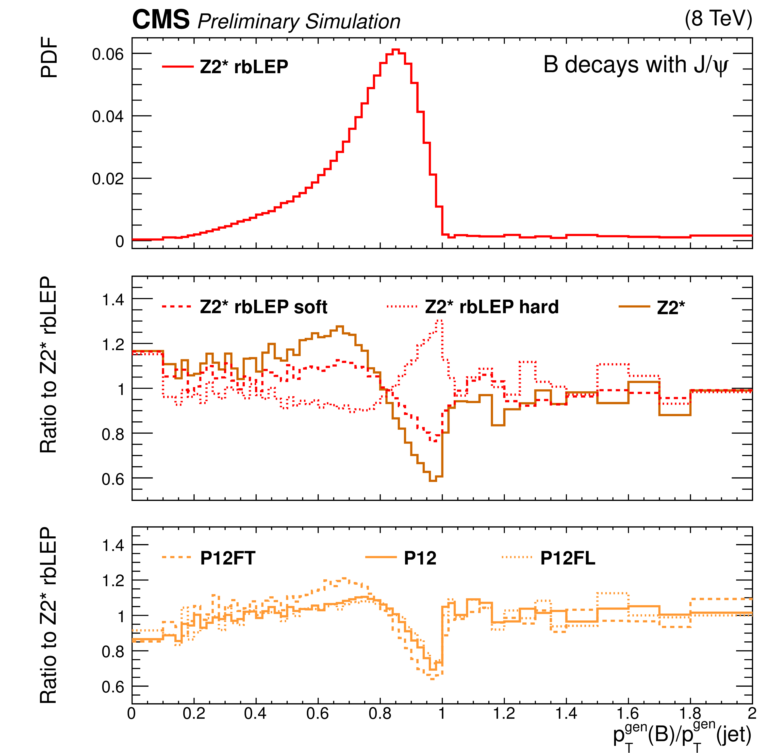
Figure 8:
Ratio of the $ {p_{\mathrm {T}}} $ of the B hadrons to the $ {p_{\mathrm {T}}} $ of the matched generator level jet for the $\mathrm {Z}2^\ast $rbLEP tune (a), the $Z2^\ast $ tune (b), and the variations of the $\mathrm {Z}2^\ast $rbLEP tune (b) and the P12 tune (c). |
png pdf |
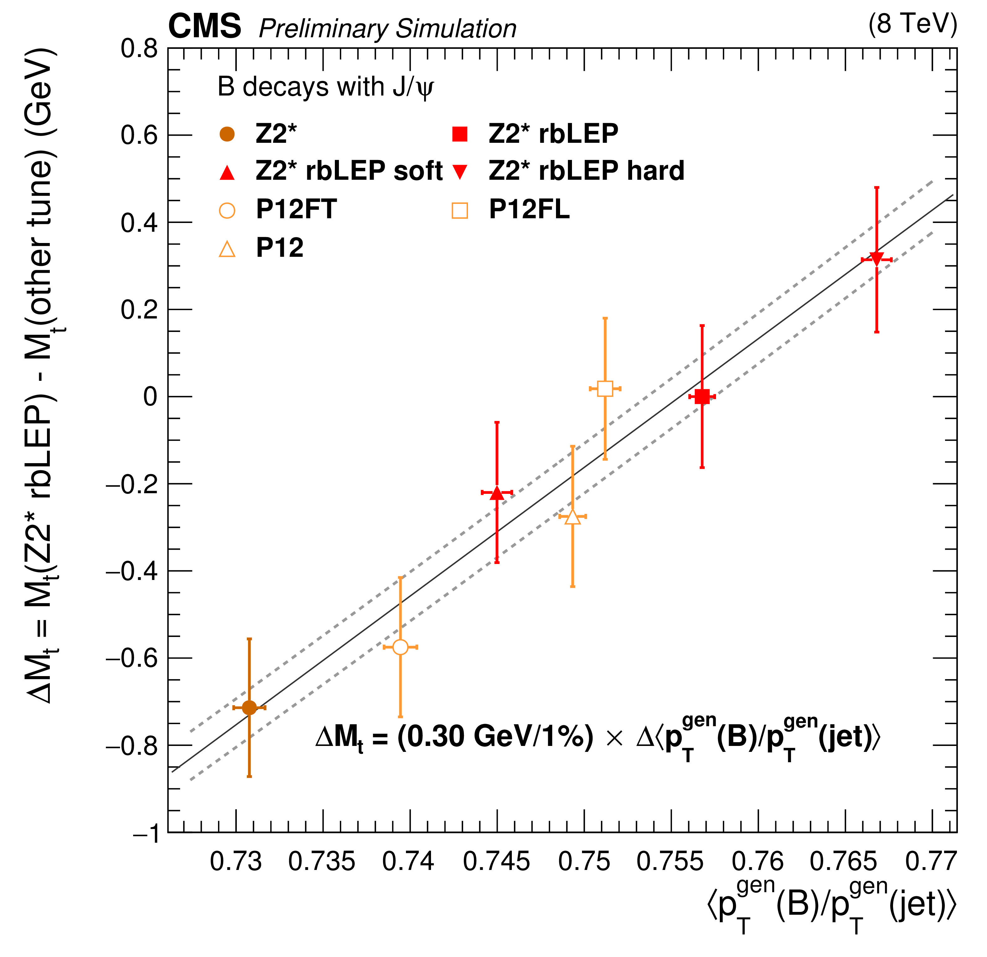
Figure 9:
Dependence of extracted $M_\mathrm {t}$ value on the average fragmentation $< {p_{\mathrm {T}}} ^\mathrm {gen}(\mathrm {B})/ {p_{\mathrm {T}}} ^\mathrm {gen}(jet) > $, fitted with a $1^\mathrm {st}$ order polynomial function. |
png pdf |
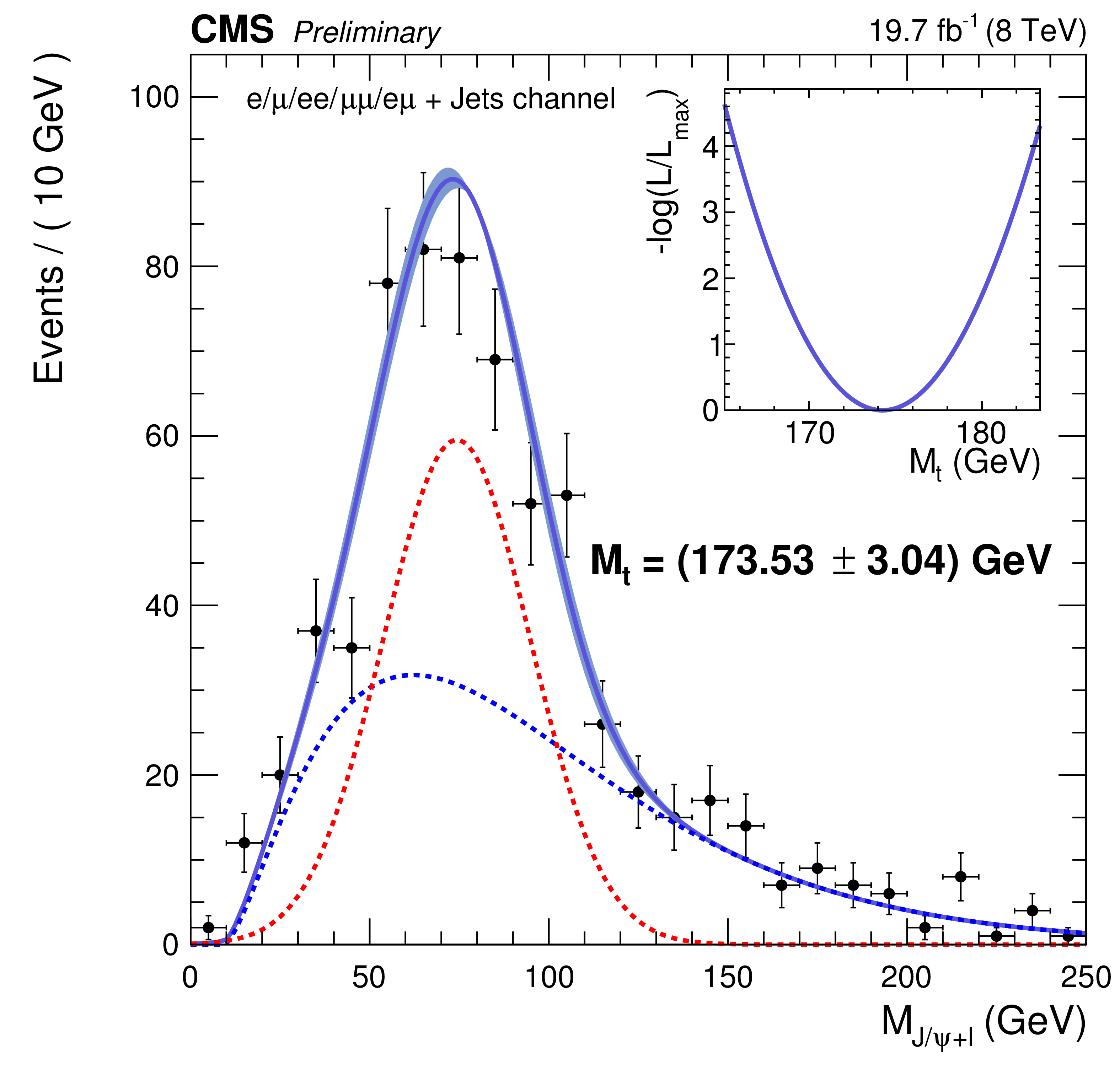
Figure 10:
Fit of the leading lepton-$ {\mathrm {J}/\psi }$ candidate invariant mass with $P_\mathrm {sig+bg}$. The inset shows the scan of the log likelihood as a function of the only free parameter which is $M_\mathrm {t}$. |
png pdf |
Figure 11-a:
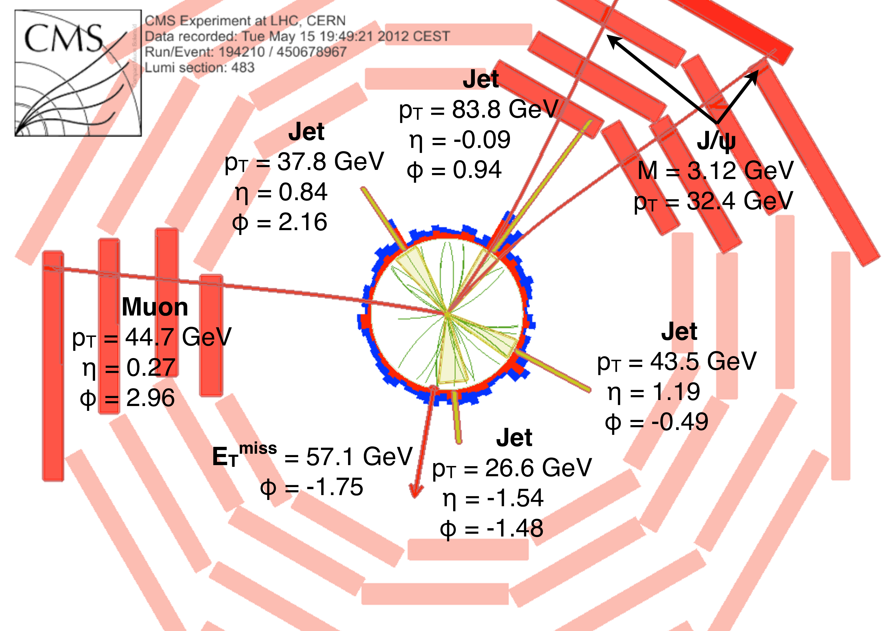
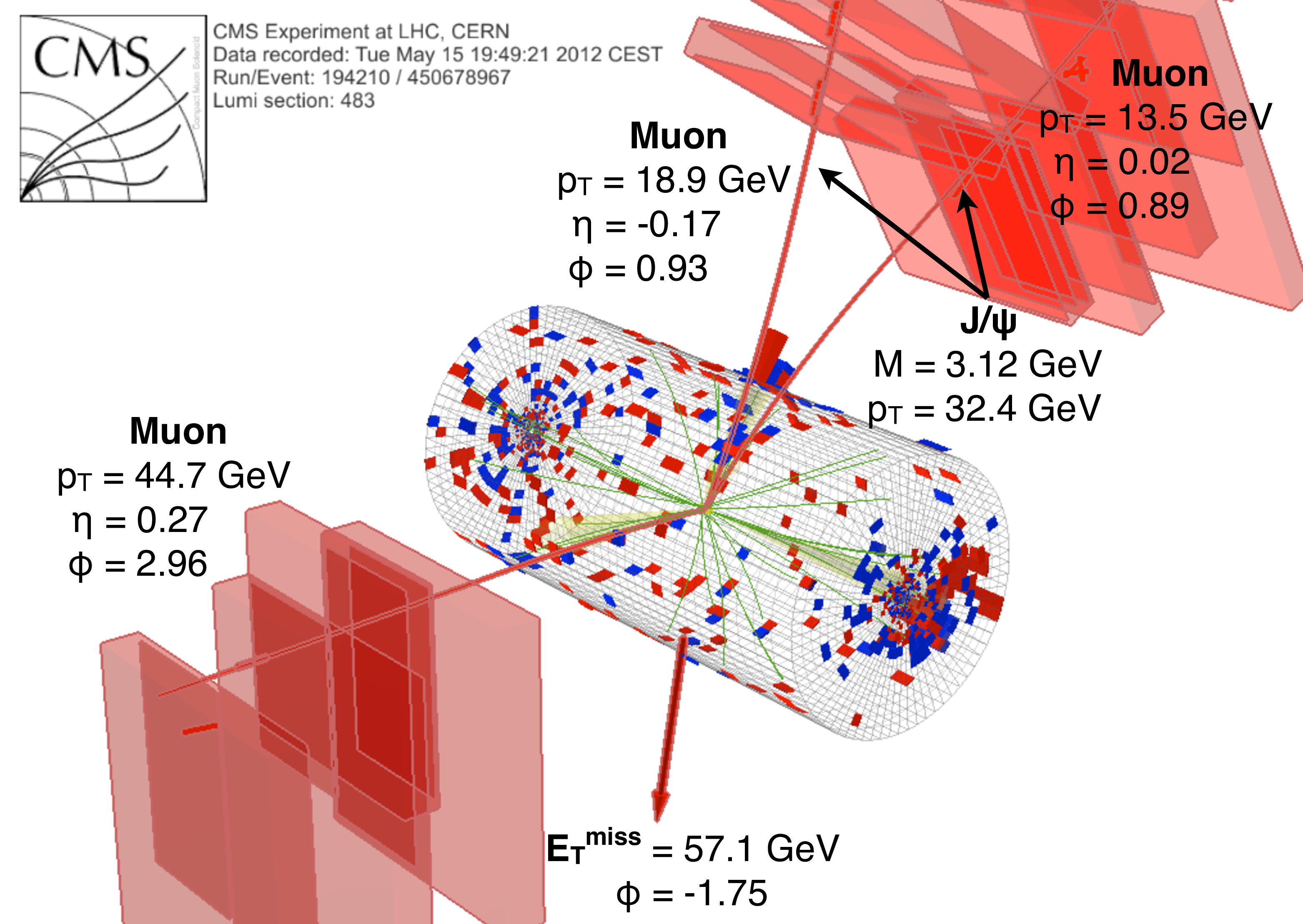
Display of the reconstructed tracks (green lines), calorimeter energy deposits (red for ECAL, blue for HCAL), jets (orange cones), muons (red lines) and missing transverse energy (red arrow) in one event selected in data, in which a pair of opposite sign secondary muons with a mass close to the $ {\mathrm {J}/\psi }$ is reconstructed within a jet. The positive and the negative muons are bent away from each other by the solenoidal magnetic field. |
png pdf |
Figure 11-b:
Display of the reconstructed tracks (green lines), calorimeter energy deposits (red for ECAL, blue for HCAL), jets (orange cones), muons (red lines) and missing transverse energy (red arrow) in one event selected in data, in which a pair of opposite sign secondary muons with a mass close to the $ {\mathrm {J}/\psi }$ is reconstructed within a jet. The positive and the negative muons are bent away from each other by the solenoidal magnetic field. |

png pdf |
Figure 11-c:
Display of the reconstructed tracks (green lines), calorimeter energy deposits (red for ECAL, blue for HCAL), jets (orange cones), muons (red lines) and missing transverse energy (red arrow) in one event selected in data, in which a pair of opposite sign secondary muons with a mass close to the $ {\mathrm {J}/\psi }$ is reconstructed within a jet. The positive and the negative muons are bent away from each other by the solenoidal magnetic field. |

png pdf |
Figure 12-a:
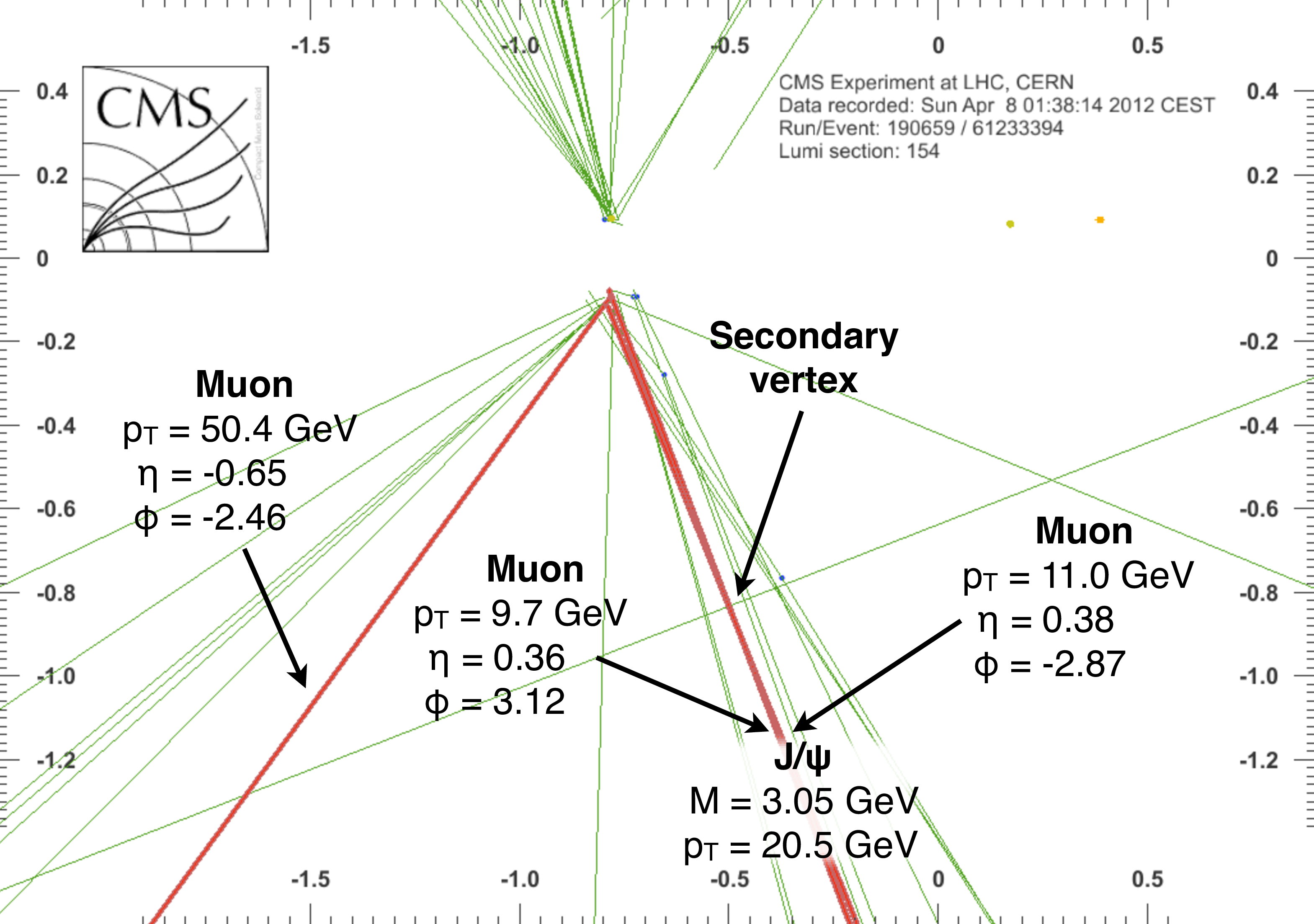
Display of the reconstructed tracks (green lines), calorimeter energy deposits (red for ECAL, blue for HCAL), jets (orange cones), muons (red lines) and missing transverse energy (red arrow) in one event selected in data, in which a pair of opposite sign secondary muons with a mass close to the $ {\mathrm {J}/\psi }$ is reconstructed within a jet. The positive and the negative muons are emitted in such a way that they are bent by the solenoidal magnetic field back together. |

png pdf |
Figure 12-b:
Display of the reconstructed tracks (green lines), calorimeter energy deposits (red for ECAL, blue for HCAL), jets (orange cones), muons (red lines) and missing transverse energy (red arrow) in one event selected in data, in which a pair of opposite sign secondary muons with a mass close to the $ {\mathrm {J}/\psi }$ is reconstructed within a jet. The positive and the negative muons are emitted in such a way that they are bent by the solenoidal magnetic field back together. |
png pdf |
Figure 12-c:
Display of the reconstructed tracks (green lines), calorimeter energy deposits (red for ECAL, blue for HCAL), jets (orange cones), muons (red lines) and missing transverse energy (red arrow) in one event selected in data, in which a pair of opposite sign secondary muons with a mass close to the $ {\mathrm {J}/\psi }$ is reconstructed within a jet. The positive and the negative muons are emitted in such a way that they are bent by the solenoidal magnetic field back together. |
| Tables | |
png pdf |
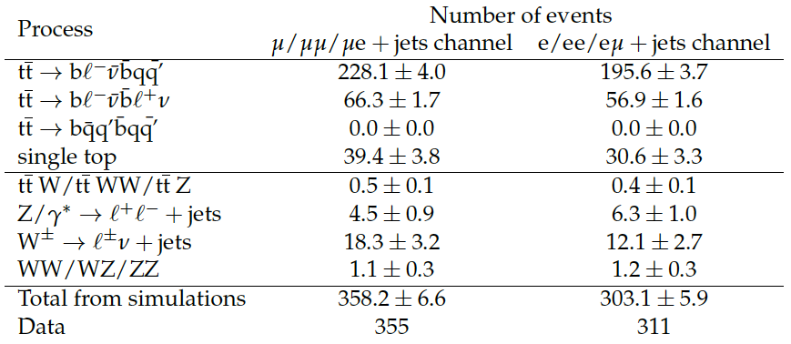
Table 1:
Number of selected events from MC simulations and observed in data for the electron and muon channels for 19.7 fb$^{-1}$. The quoted uncertainties are of statistical nature. |
png pdf |
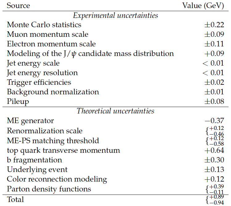
Table 2:
Summary of the systematic uncertainties on the top quark mass for each source. |
|
|
Compact Muon Solenoid LHC, CERN |
|

|

|

|

|

|