CMS-PAS-SUS-15-007

CMS-PAS-SUS-15-007
Search for supersymmetry in pp collisions at $\sqrt s =$ 13 TeV in the single-lepton final state using the sum of masses of large radius jets
CMS Collaboration
December 2015

Abstract: Results are reported from a search for supersymmetric particles in pp collisions in the final state with a single, high $p_{\rm T}$ lepton; multiple jets, including at least one b-tagged jet; and large missing transverse momentum. The data sample corresponds to 2.1 fb $^{-1}$ recorded by the CMS experiment at $\sqrt s=$ 13 TeV. The search focuses on processes leading to high jet multiplicities, such as ${\rm gg}\to{\rm \tilde g\tilde g}$ with ${\rm \tilde g}\to{\rm t}{\rm \bar t}\,{\tilde\chi^0_1}$ . The quantity $M_J$ , defined as the sum of the masses of the large-radius jets in the event, is used in conjunction with other kinematic variables to provide discrimination between signal and backgrounds and as a key part of the background estimation method. The observed event yields in the signal regions in data are consistent with those expected for standard model backgrounds, which are estimated from control regions. Exclusion limits are obtained for the simplified model T1tttt, which corresponds to gluino pair production with decays into top quarks plus neutralinos. Gluinos with mass below 1575 GeV are excluded at 95\% CL for T1tttt scenarios with low $\tilde\chi_1^0$ mass.
Links: CDS record (PDF) ; CADI line (restricted) ; These preliminary results are superseded in this paper, JHEP 08 (2016) 122. The superseded preliminary plots can be found here.

Figures
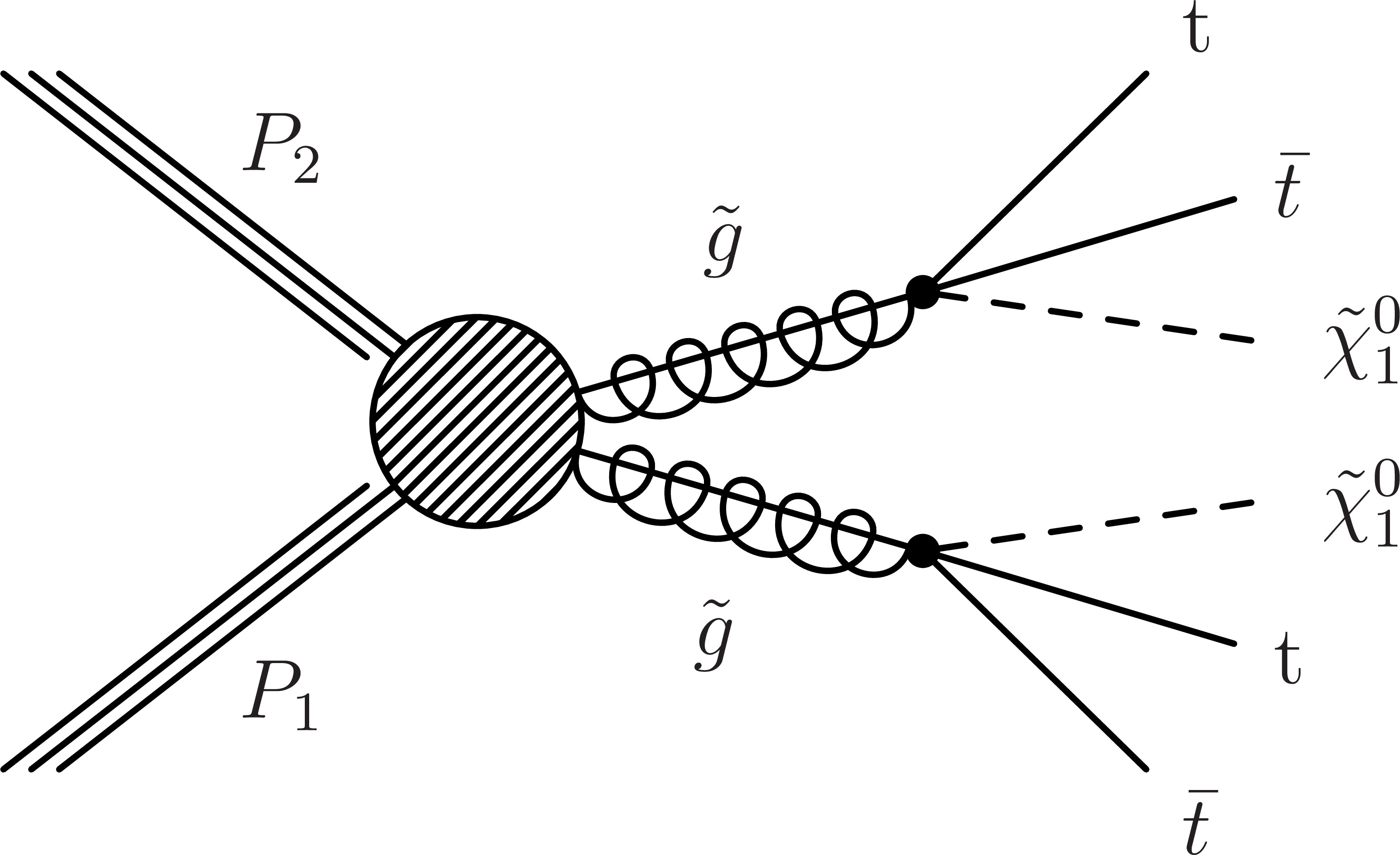
png ; pdf ;	Figure 1: Gluino pair production and decay for the simplified model T1tttt.
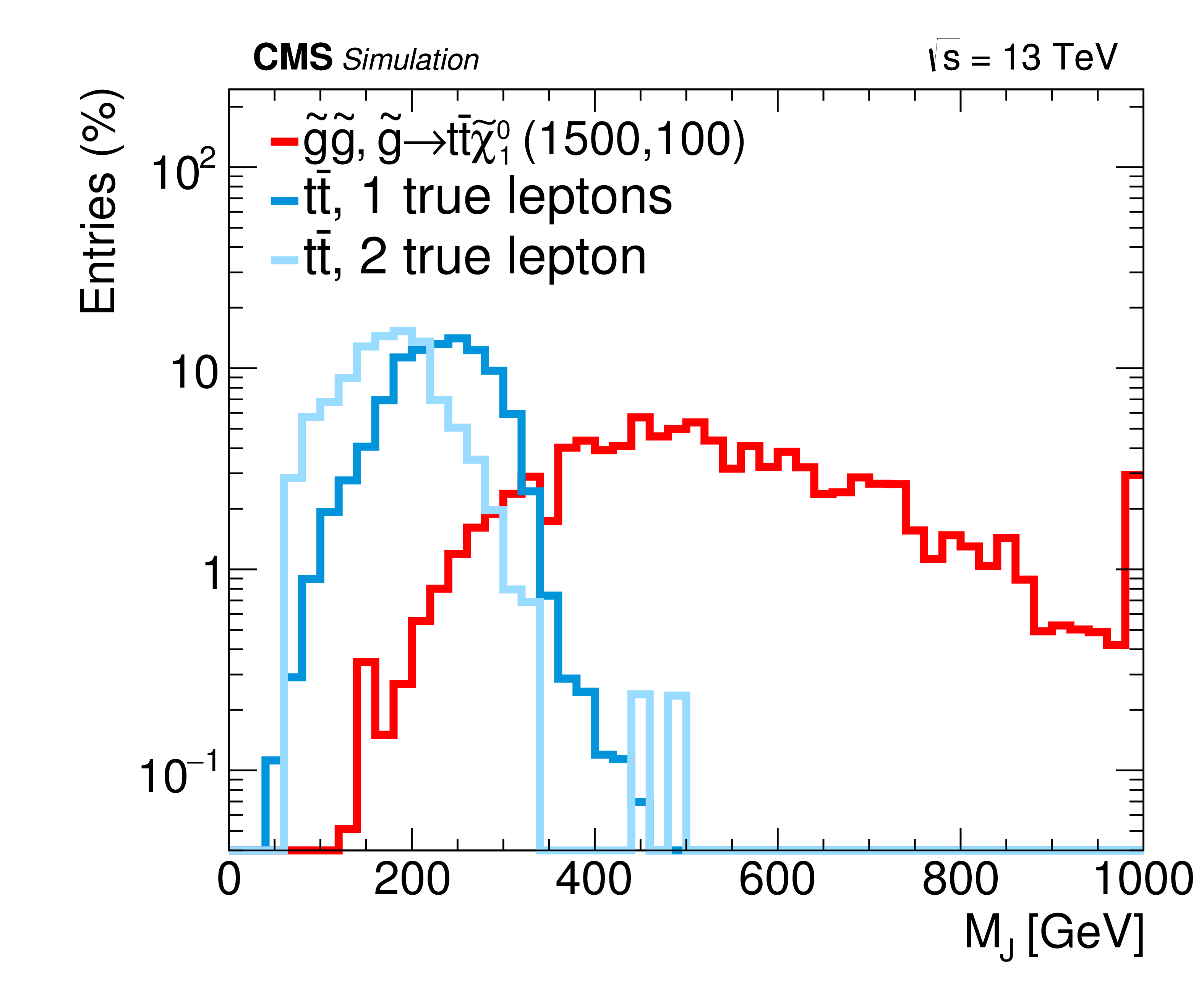
png ; pdf ;	Figure 2-a: Distributions of ${M_J}$ from simulated event samples with little ISR (a), and significant ISR (b). The amount of ISR is selected using the ${p_{\mathrm {T}}}$ of the $\mathrm{ t \bar{t} }$ or gluino-gluino system. The distributions are shown for $\mathrm{ t \bar{t} }$ single- and dilepton events and for a T1tttt SUSY model with a 1500 GeV gluino and a 100 GeV neutralino. When the ISR contribution is small, the ${M_J}$ distribution for $\mathrm{ t \bar{t} }$ events has a cutoff around $2m_{\rm t}$ (blue curves in the left-hand plot). If the ISR contribution is substantial, this tail is greatly extended (blue curves in the right-hand plot. The signal events have a large tail in the ${M_J}$ distribution regardless of the amount of ISR. For each distribution, the mean value ( $\mu$ ) is given in the legend.
png ; pdf ;	Figure 2-b: Distributions of ${M_J}$ from simulated event samples with little ISR (a), and significant ISR (b). The amount of ISR is selected using the ${p_{\mathrm {T}}}$ of the $\mathrm{ t \bar{t} }$ or gluino-gluino system. The distributions are shown for $\mathrm{ t \bar{t} }$ single- and dilepton events and for a T1tttt SUSY model with a 1500 GeV gluino and a 100 GeV neutralino. When the ISR contribution is small, the ${M_J}$ distribution for $\mathrm{ t \bar{t} }$ events has a cutoff around $2m_{\rm t}$ (blue curves in the left-hand plot). If the ISR contribution is substantial, this tail is greatly extended (blue curves in the right-hand plot. The signal events have a large tail in the ${M_J}$ distribution regardless of the amount of ISR. For each distribution, the mean value ( $\mu$ ) is given in the legend.
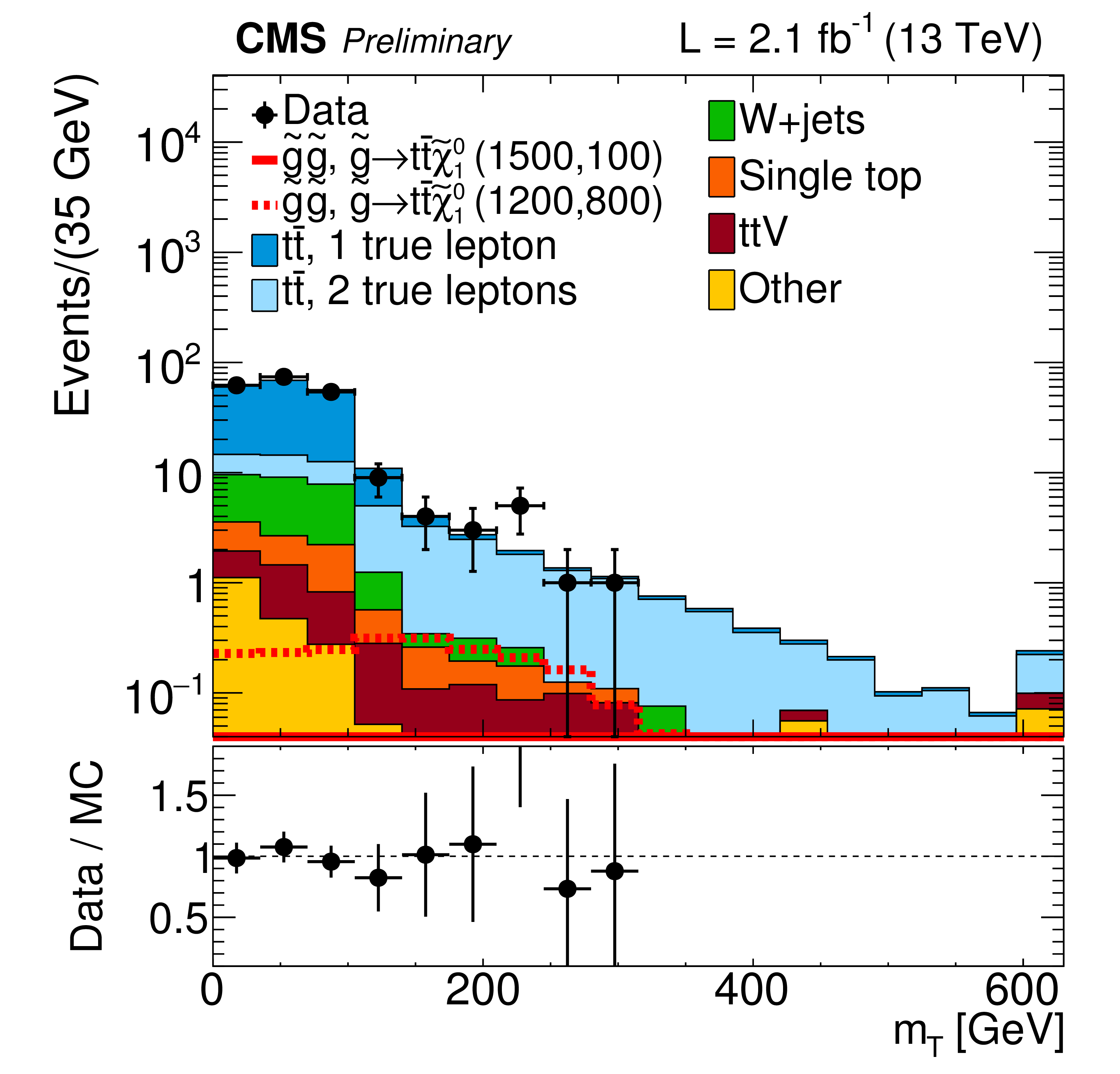
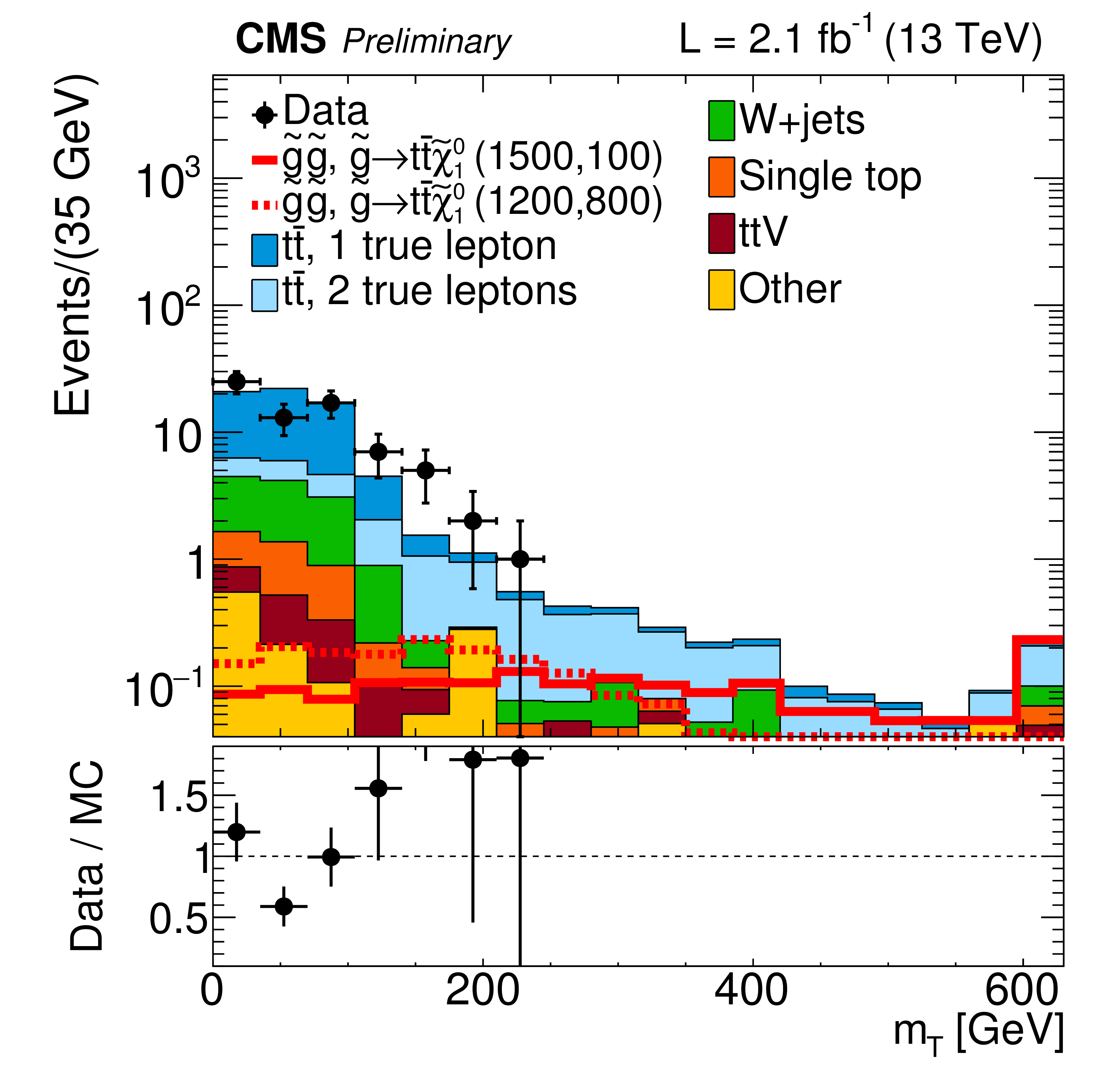
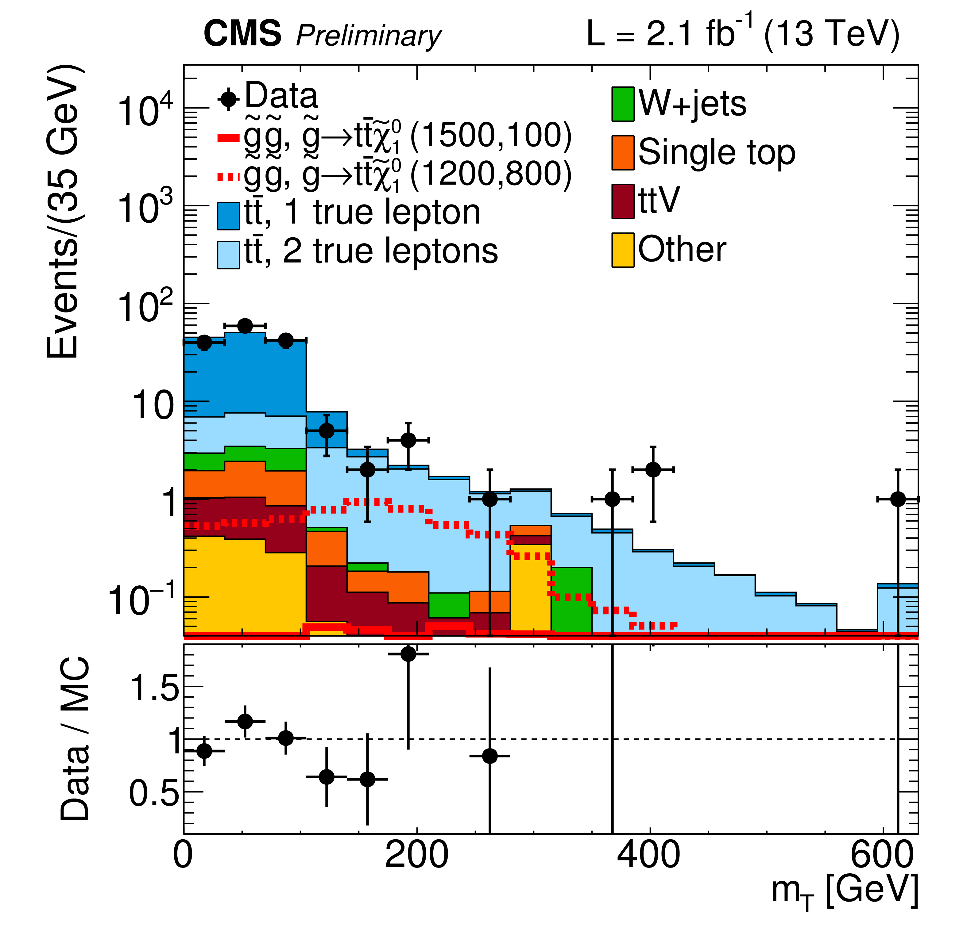
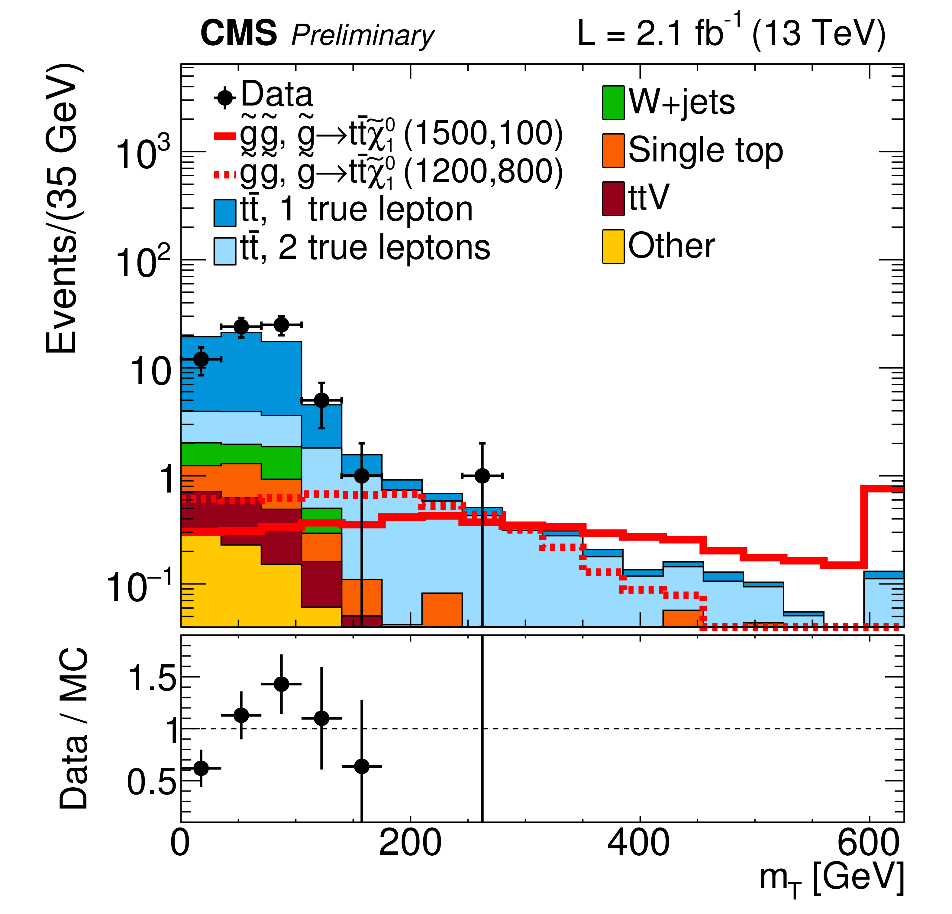
png ; pdf ;	Figure 3-a: Distributions of ${m_{\mathrm {T}}}$ after the baseline selection is applied (a) and ${M_J}$ after the baseline selection and the requirement ${m_{\mathrm {T}}} >$ 140 GeV are applied (b).
png ; pdf ;	Figure 3-b: Distributions of ${m_{\mathrm {T}}}$ after the baseline selection is applied (a) and ${M_J}$ after the baseline selection and the requirement ${m_{\mathrm {T}}} >$ 140 GeV are applied (b).
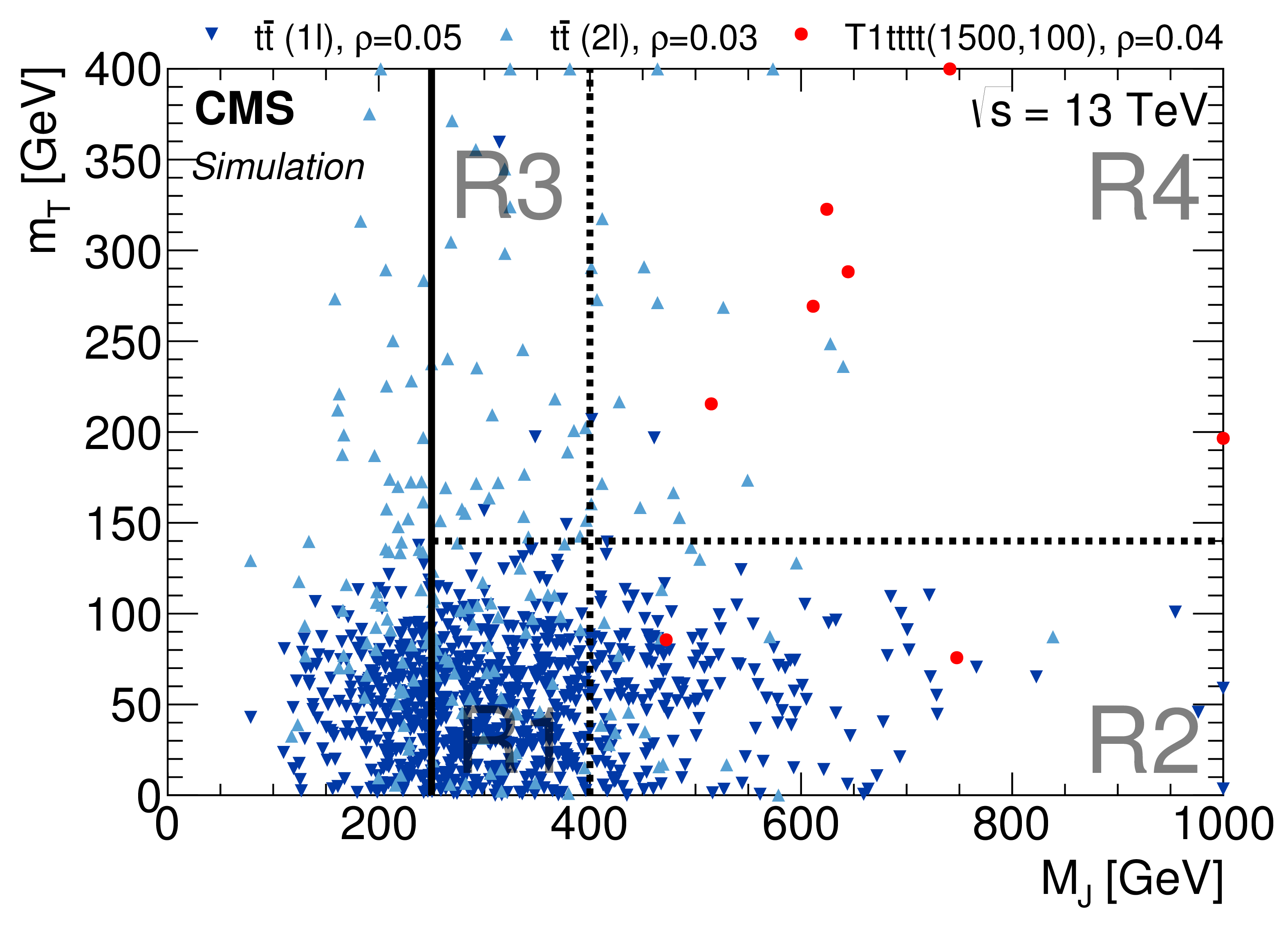
png ; pdf ;	Figure 4: Distribution of single lepton $\mathrm{ t \bar{t} }$ , dilepton $\mathrm{ t \bar{t} }$ , and T1tttt(1500,100) events in the ${M_J}$ - ${m_{\mathrm {T}}}$ plane after baseline selection. Each marker represents one expected event at ${\cal L}=$ 3 fb ${-1}$ . The correlation coefficients $\rho$ are shown in the legend.
png ; pdf ;	Figure 5: Binning used in the signal (R4) and control regions (R1, R2, and R3) of the analysis. The low ${M_J}$ region R1 and R3 are divided only into low and high MET regions. Because of the correlation with ${m_{\mathrm {T}}}$ , binning in MET is necessary in the low ${M_J}$ sideband to obtain the correct ${m_{\mathrm {T}}}$ shape. At high ${M_J}$ , we partition regions R2 and R4 into 10 bins each using ${N_{\text {jets}}}$ , ${N_{\text {b}}}$ , and ${E_{\mathrm {T}}^{\text {miss}}}$ .
png ; pdf ;	Figure 6-a: a: comparison of ${M_J}$ distribution in $\mathrm{ t \bar{t} }$ events with 2 true leptons at high and low ${m_{\mathrm {T}}}$ . Shapes are similar. 2 $\ell$ $\mathrm{ t \bar{t} }$ is subdominant at low ${m_{\mathrm {T}}}$ . b: comparison of ${M_J}$ distribution in $\mathrm{ t \bar{t} }$ events with 1 true lepton at high and low ${m_{\mathrm {T}}}$ . Shapes are rather different which can introduce a correlation between ${M_J}$ and ${m_{\mathrm {T}}}$ . However, the single lepton component of the high- ${m_{\mathrm {T}}}$ background is small, approximately 15% of the full sample. c: comparison of ${M_J}$ distribution in $\mathrm{ t \bar{t} }$ events with 2 true leptons at high ${m_{\mathrm {T}}}$ and 1 true lepton at low ${m_{\mathrm {T}}}$ . The shapes of these distributions are similar. These two are the dominant contributions to each of their respective ${m_{\mathrm {T}}}$ regions.
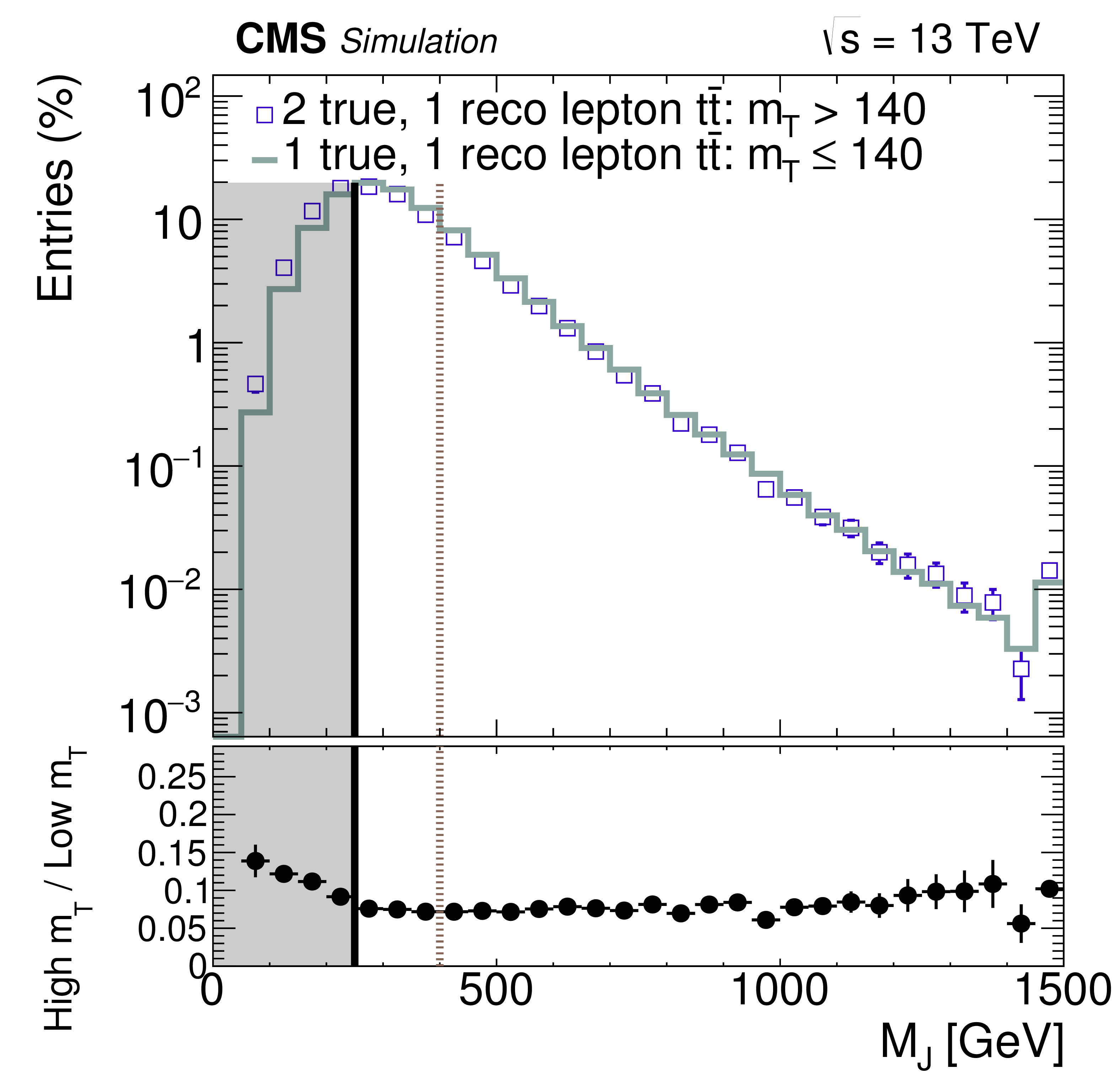
png ; pdf ;	Figure 6-b: a: comparison of ${M_J}$ distribution in $\mathrm{ t \bar{t} }$ events with 2 true leptons at high and low ${m_{\mathrm {T}}}$ . Shapes are similar. 2 $\ell$ $\mathrm{ t \bar{t} }$ is subdominant at low ${m_{\mathrm {T}}}$ . b: comparison of ${M_J}$ distribution in $\mathrm{ t \bar{t} }$ events with 1 true lepton at high and low ${m_{\mathrm {T}}}$ . Shapes are rather different which can introduce a correlation between ${M_J}$ and ${m_{\mathrm {T}}}$ . However, the single lepton component of the high- ${m_{\mathrm {T}}}$ background is small, approximately 15% of the full sample. c: comparison of ${M_J}$ distribution in $\mathrm{ t \bar{t} }$ events with 2 true leptons at high ${m_{\mathrm {T}}}$ and 1 true lepton at low ${m_{\mathrm {T}}}$ . The shapes of these distributions are similar. These two are the dominant contributions to each of their respective ${m_{\mathrm {T}}}$ regions.
png ; pdf ;	Figure 6-c: a: comparison of ${M_J}$ distribution in $\mathrm{ t \bar{t} }$ events with 2 true leptons at high and low ${m_{\mathrm {T}}}$ . Shapes are similar. 2 $\ell$ $\mathrm{ t \bar{t} }$ is subdominant at low ${m_{\mathrm {T}}}$ . b: comparison of ${M_J}$ distribution in $\mathrm{ t \bar{t} }$ events with 1 true lepton at high and low ${m_{\mathrm {T}}}$ . Shapes are rather different which can introduce a correlation between ${M_J}$ and ${m_{\mathrm {T}}}$ . However, the single lepton component of the high- ${m_{\mathrm {T}}}$ background is small, approximately 15% of the full sample. c: comparison of ${M_J}$ distribution in $\mathrm{ t \bar{t} }$ events with 2 true leptons at high ${m_{\mathrm {T}}}$ and 1 true lepton at low ${m_{\mathrm {T}}}$ . The shapes of these distributions are similar. These two are the dominant contributions to each of their respective ${m_{\mathrm {T}}}$ regions.
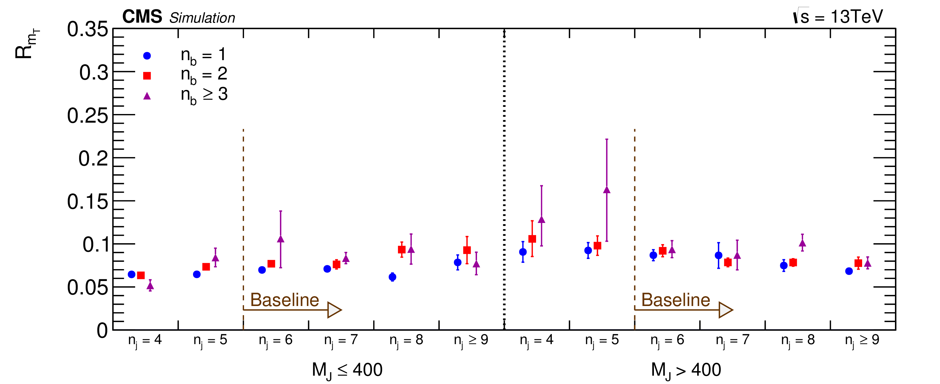
png ; pdf ;	Figure 7: The high-to-low- ${m_{\mathrm {T}}}$ ratio $R_{ {m_{\mathrm {T}}} }$ at low ${E_{\mathrm {T}}^{\text {miss}}}$ as a function of ${N_{\text {jets}}}$ and ${N_{\text {b}}}$ , showing that $R_{ {m_{\mathrm {T}}} }$ varies slowly from approximately 0.06 to 0.1.
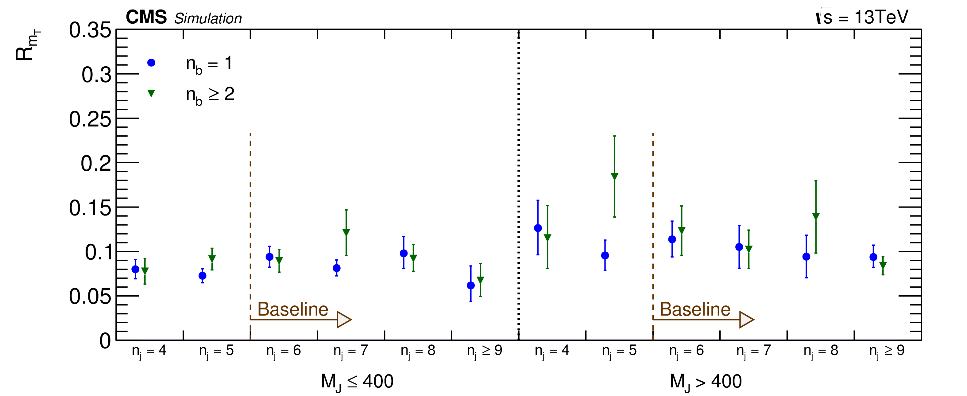
png ; pdf ;	Figure 8: The high-to-low- ${m_{\mathrm {T}}}$ ratio $R_{ {m_{\mathrm {T}}} }$ at high ${E_{\mathrm {T}}^{\text {miss}}}$ as a function of ${N_{\text {jets}}}$ and ${N_{\text {b}}}$ , showing that $R_{ {m_{\mathrm {T}}} }$ varies slowly from approximately 0.08 to 0.12, slightly higher than the values in Figure 7. The difference between the two figures indicates a ${E_{\mathrm {T}}^{\text {miss}}}$ dependence in $R_{ {m_{\mathrm {T}}} }$ .
png ; pdf ;	Figure 9: Double-ratio $\kappa$ in various kinematic bins defined in section 4. $\kappa$ is generally consistent with one, with the largest discrepancy in the bin with the tightest selection, ${E_{\mathrm {T}}^{\text {miss}}} >$ 400 and ${N_{\text {jets}}} \geq$ 9.
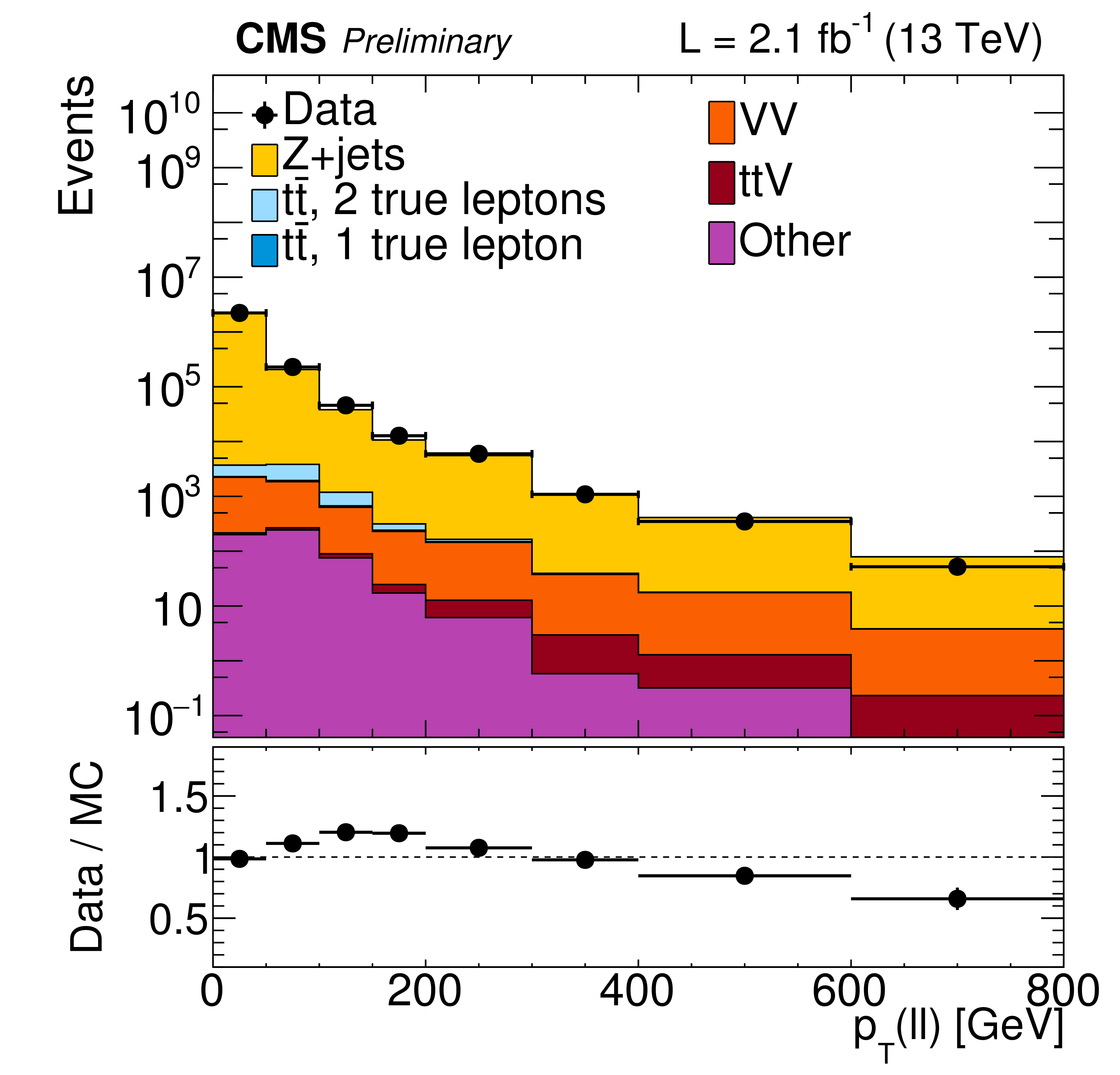
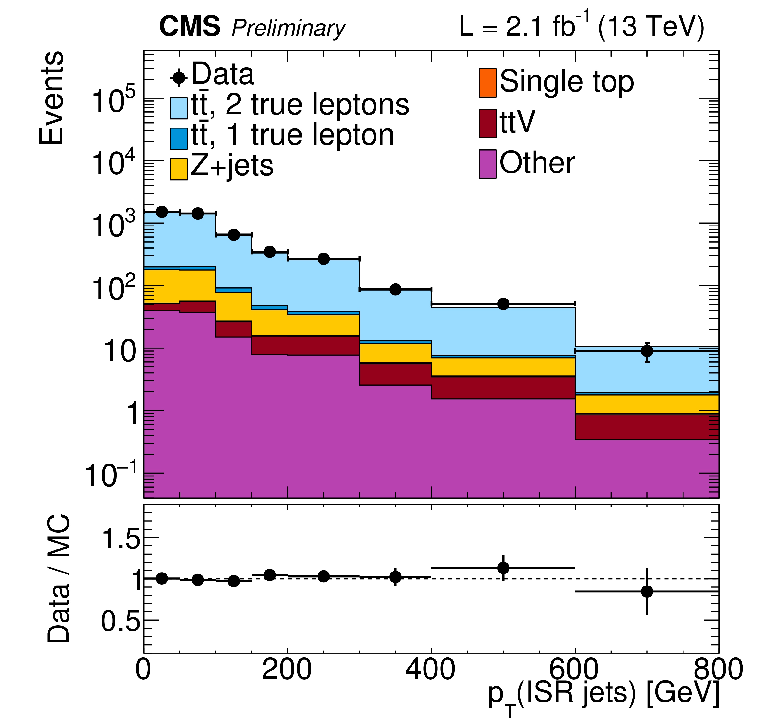
png ; pdf ;	Figure 10-a: The ISR ${p_{\mathrm {T}}}$ in ${\mathrm {Z+jets}}$ sample (a) and a dilepton $\mathrm{ t \bar{t} }$ sample (b).
png ; pdf ;	Figure 10-b: The ISR ${p_{\mathrm {T}}}$ in ${\mathrm {Z+jets}}$ sample (a) and a dilepton $\mathrm{ t \bar{t} }$ sample (b).
png ; pdf ;	Figure 11: Uncertainty measurement using the dilepton sample in data (2.1 fb $^{-1}$ ). Distribution of ${M_J}$ for single-lepton ${m_{\mathrm {T}}} <$ 140 GeV (blue histogram) and di-lepton events (black points with error bars). The overall yield from the singe-lepton events is normalized to that for the di-lepton sample to compare shapes.
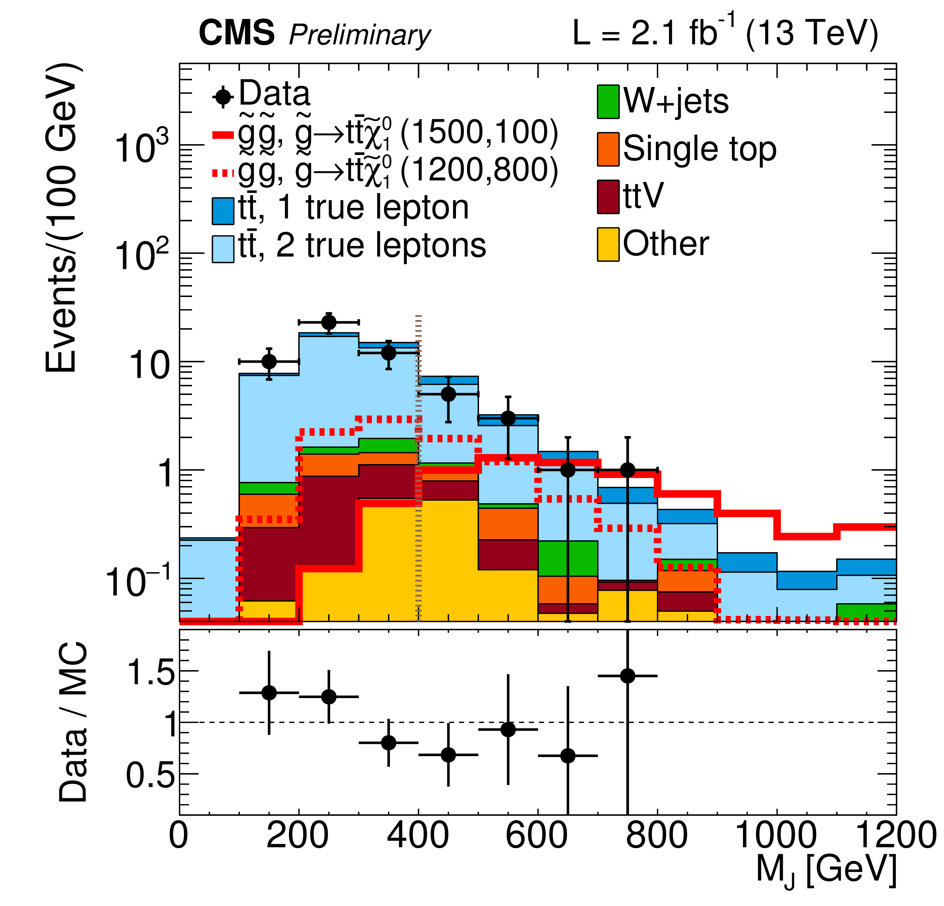
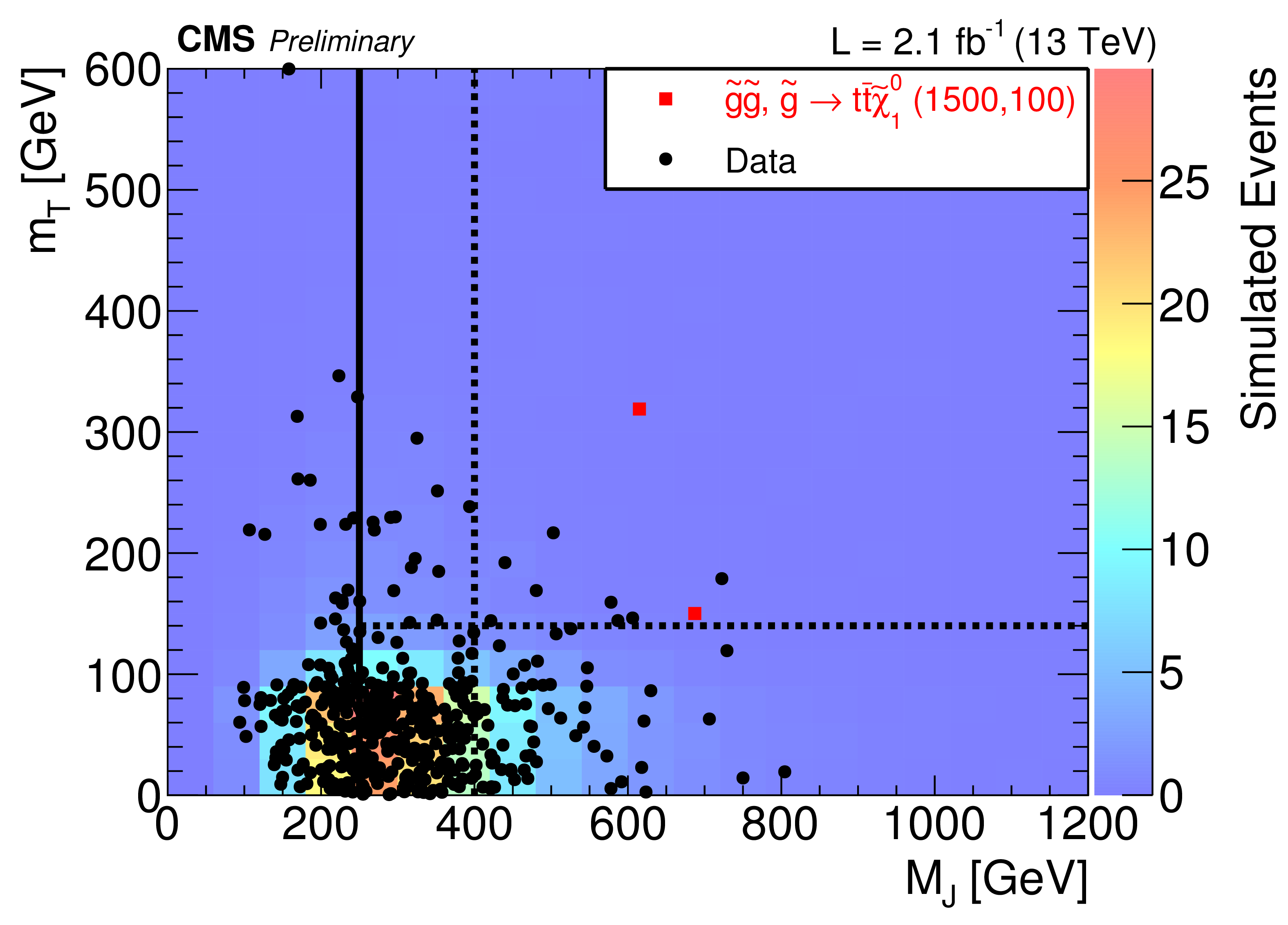
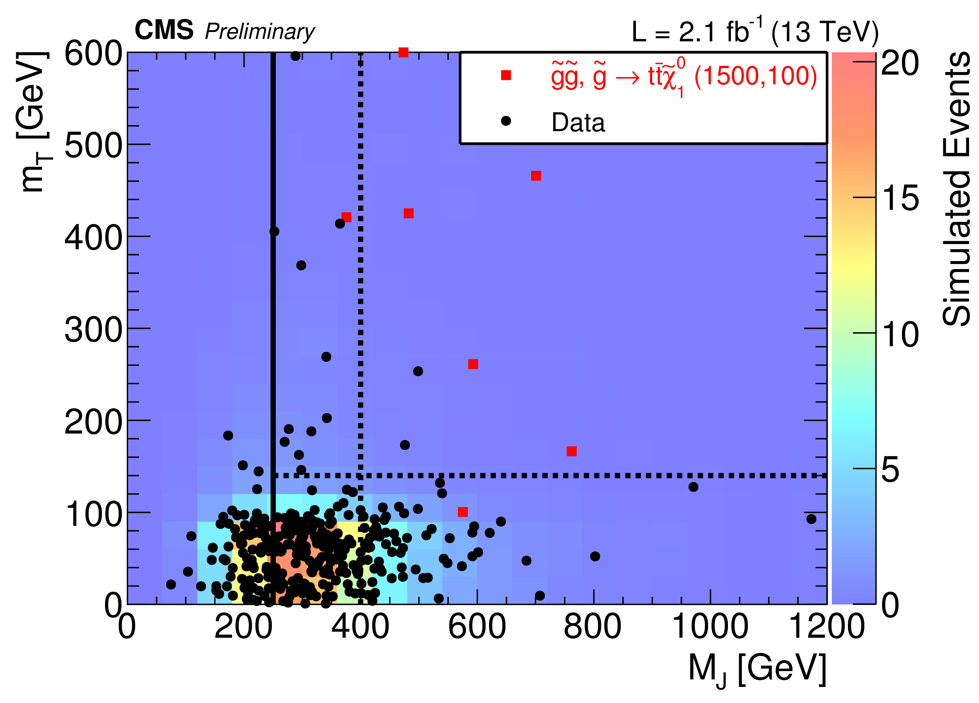
png ; pdf ;	Figure 12-a: Two-dimensional distributions of ${m_{\mathrm {T}}}$ and ${M_J}$ with ${N_{\text {b}}} =$ 1 (a) and ${N_{\text {b}}} \ge$ 2 (b) after the baseline selection. The colored histogram is all simulated background normalized to the data, the black dots are data, and the red dots are the expected T1tttt(1500,100) yield for 2.1 fb $^{-1}$ .
png ; pdf ;	Figure 12-b: Two-dimensional distributions of ${m_{\mathrm {T}}}$ and ${M_J}$ with ${N_{\text {b}}} =$ 1 (a) and ${N_{\text {b}}} \ge$ 2 (b) after the baseline selection. The colored histogram is all simulated background normalized to the data, the black dots are data, and the red dots are the expected T1tttt(1500,100) yield for 2.1 fb $^{-1}$ .
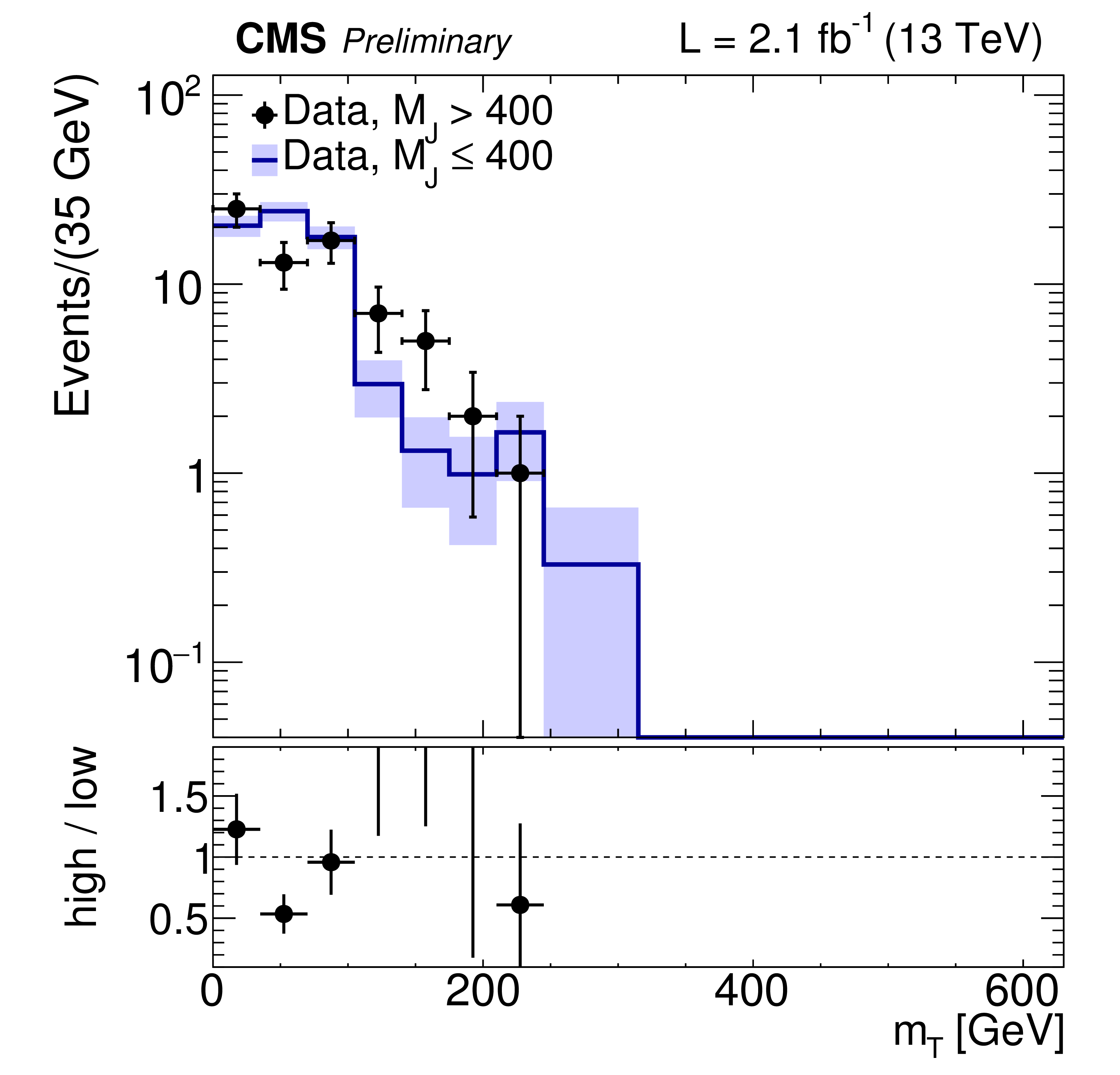
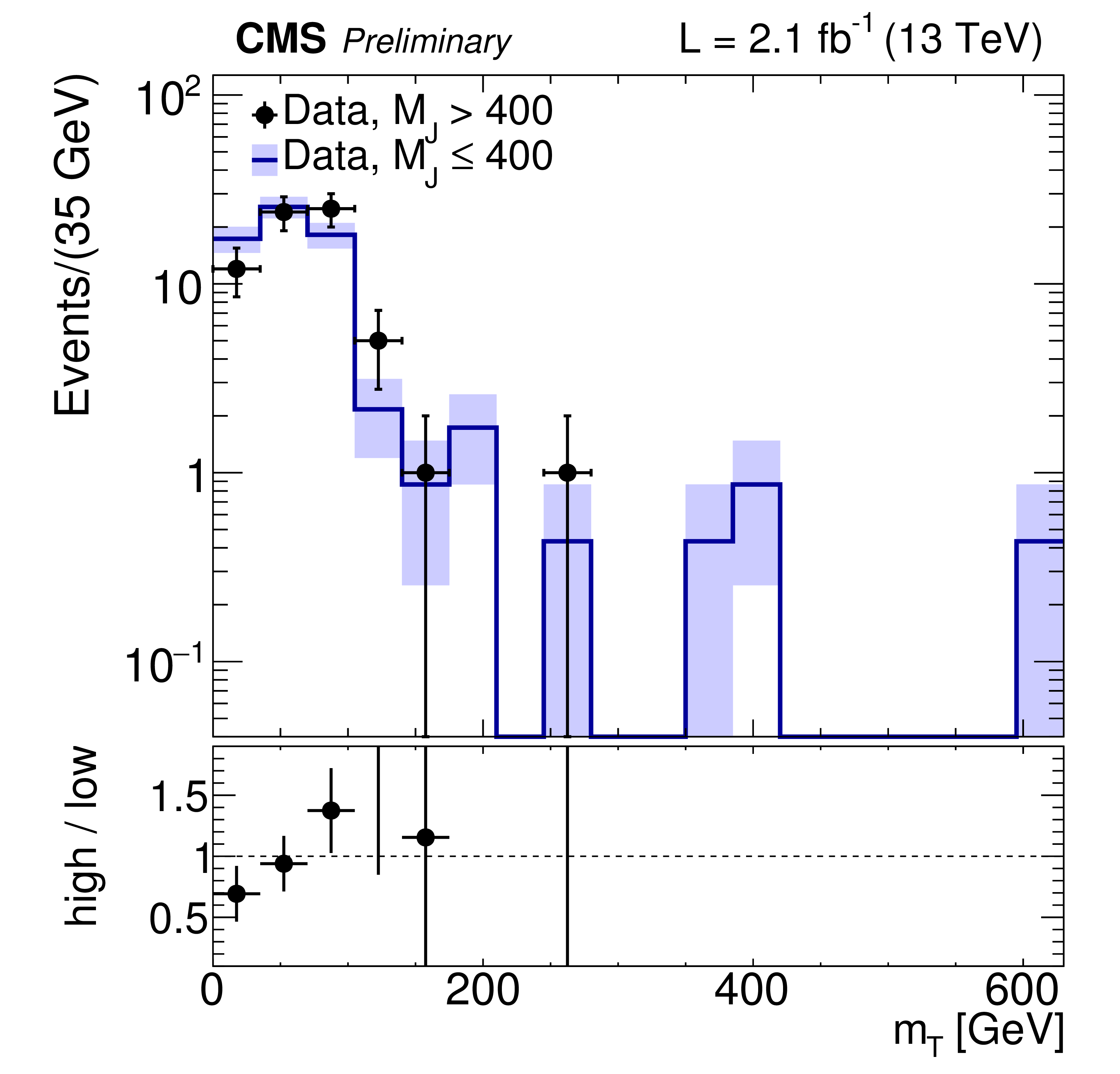
png ; pdf ;	Figure 13-a: Distributions of ${m_{\mathrm {T}}}$ for events with ${N_{\text {b}}} =$ 1 in data and simulated event samples (MC). a,b: ${m_{\mathrm {T}}}$ distributions for 250 $< {M_J} \leq$ 400 GeV (a) and ${M_J} >$ 400 GeV (b). The overall MC event yields are normalized to that in the data. c: comparison of the ${m_{\mathrm {T}}}$ distributions for low and high ${M_J}$ in data, the former normalized to the number of events in the latter. The uncertainties on the ratio plots include the uncertainties from the numerator and denominator added in quadrature.
png ; pdf ;	Figure 13-b: Distributions of ${m_{\mathrm {T}}}$ for events with ${N_{\text {b}}} =$ 1 in data and simulated event samples (MC). a,b: ${m_{\mathrm {T}}}$ distributions for 250 $< {M_J} \leq$ 400 GeV (a) and ${M_J} >$ 400 GeV (b). The overall MC event yields are normalized to that in the data. c: comparison of the ${m_{\mathrm {T}}}$ distributions for low and high ${M_J}$ in data, the former normalized to the number of events in the latter. The uncertainties on the ratio plots include the uncertainties from the numerator and denominator added in quadrature.
png ; pdf ;	Figure 13-c: Distributions of ${m_{\mathrm {T}}}$ for events with ${N_{\text {b}}} =$ 1 in data and simulated event samples (MC). a,b: ${m_{\mathrm {T}}}$ distributions for 250 $< {M_J} \leq$ 400 GeV (a) and ${M_J} >$ 400 GeV (b). The overall MC event yields are normalized to that in the data. c: comparison of the ${m_{\mathrm {T}}}$ distributions for low and high ${M_J}$ in data, the former normalized to the number of events in the latter. The uncertainties on the ratio plots include the uncertainties from the numerator and denominator added in quadrature.
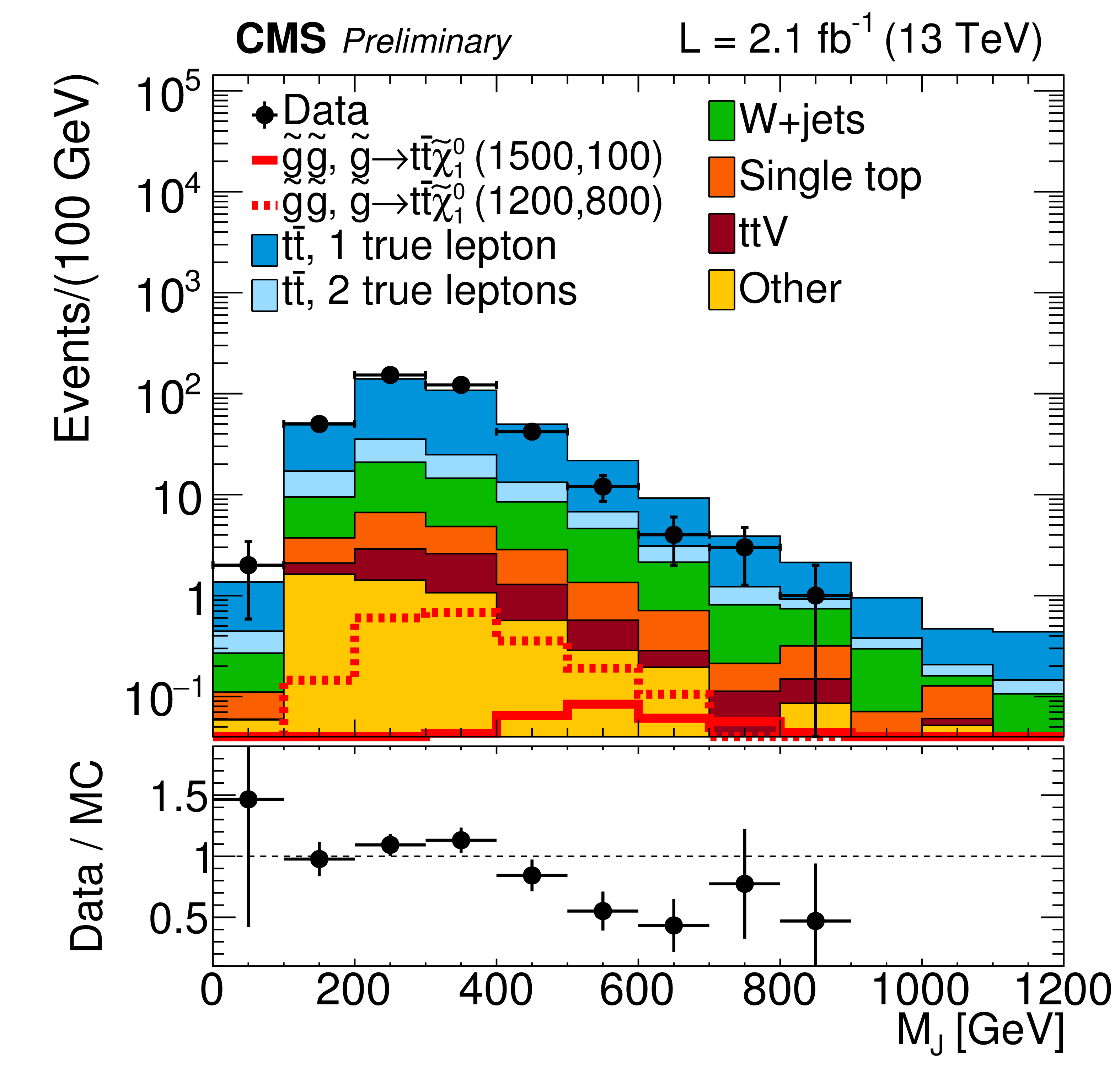
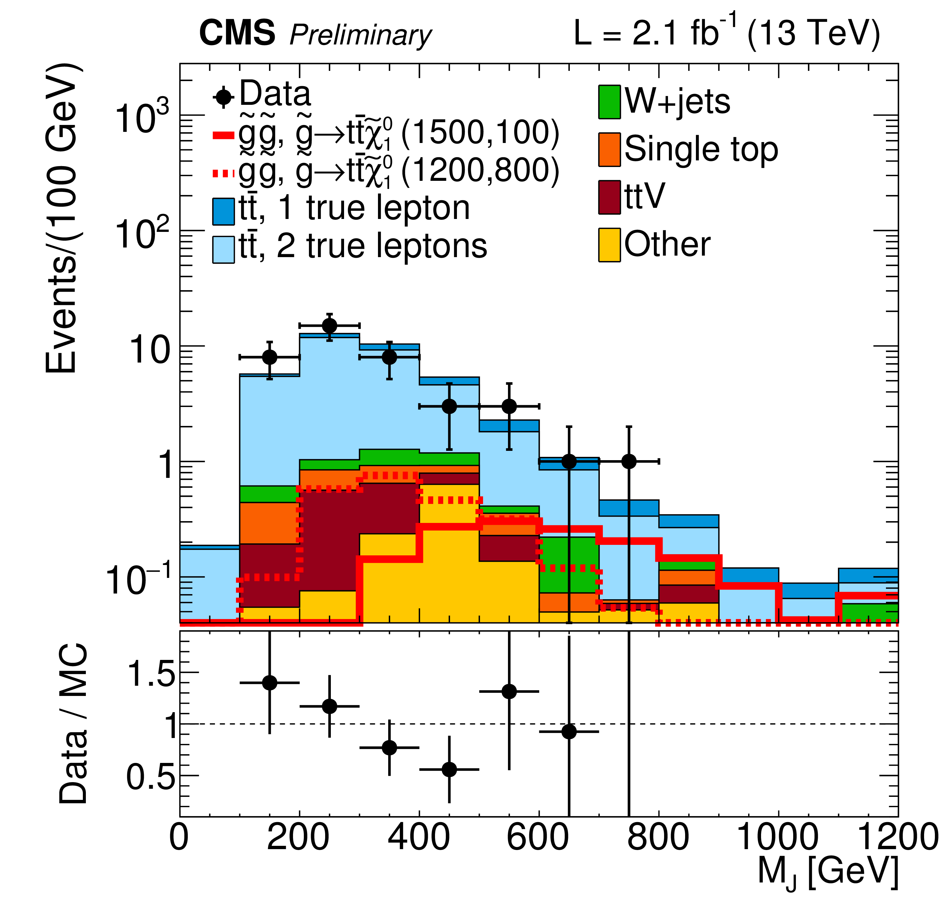
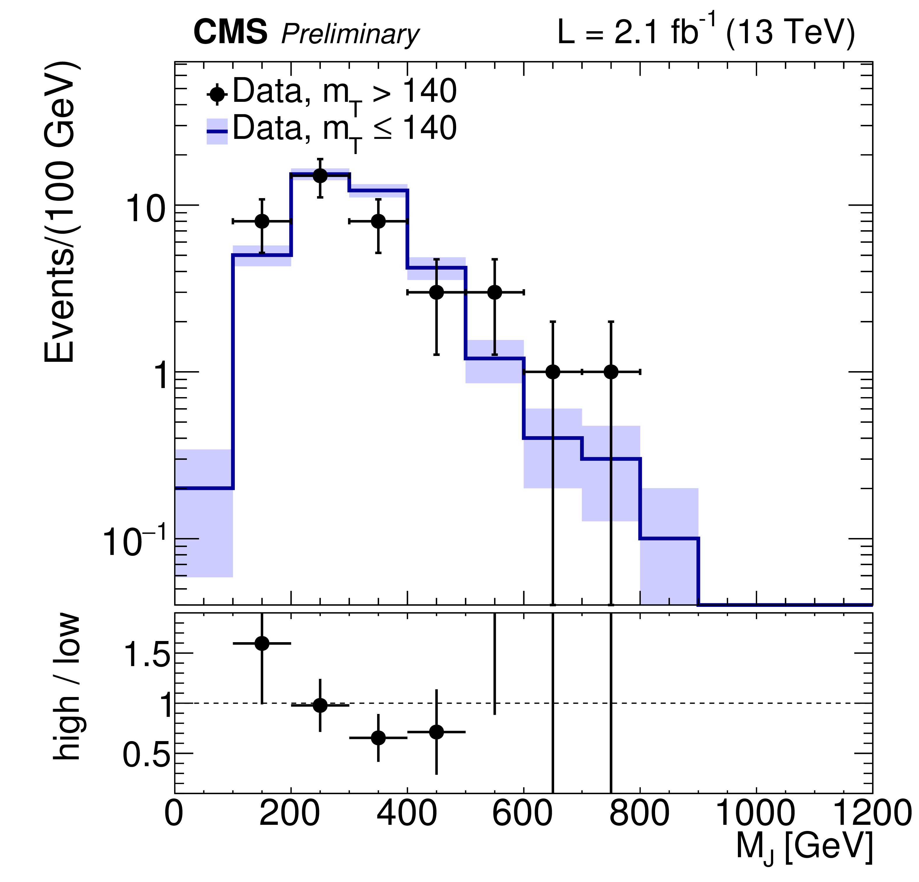
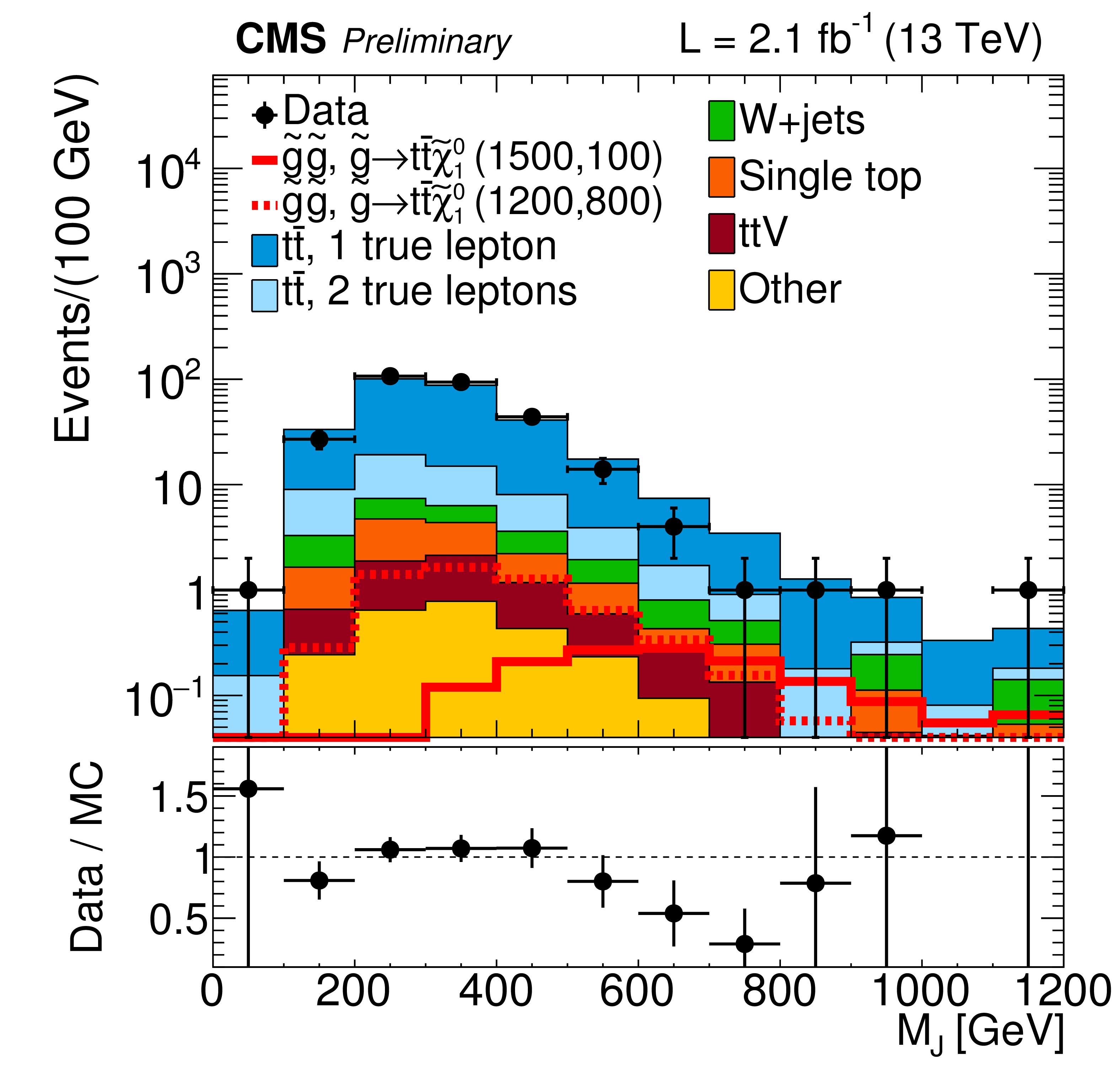
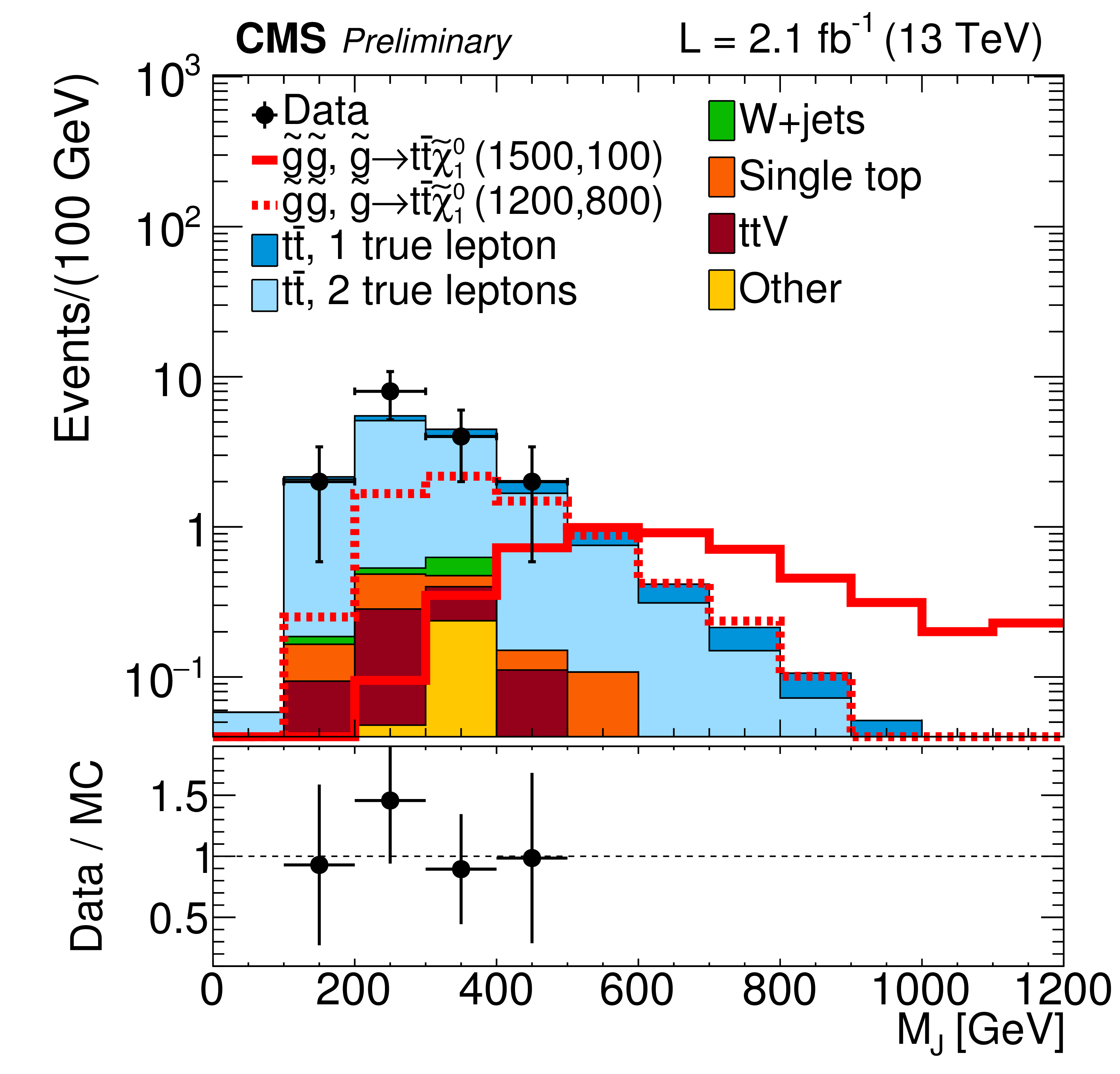
png ; pdf ;	Figure 14-a: Distributions of ${M_J}$ for events with ${N_{\text {b}}} =$ 1 in data and simulated event samples (MC). a,b: ${M_J}$ distributions for ${m_{\mathrm {T}}} \leq$ 140 GeV (a) and ${m_{\mathrm {T}}} >$ 140 GeV (b). The overall MC event yields are normalized to that in the data. c: comparison of the ${M_J}$ distributions for low and high ${m_{\mathrm {T}}}$ in data, the former normalized to the number of events in the latter. The uncertainties on the ratio plots include the uncertainties from the numerator and denominator added in quadrature.
png ; pdf ;	Figure 14-b: Distributions of ${M_J}$ for events with ${N_{\text {b}}} =$ 1 in data and simulated event samples (MC). a,b: ${M_J}$ distributions for ${m_{\mathrm {T}}} \leq$ 140 GeV (a) and ${m_{\mathrm {T}}} >$ 140 GeV (b). The overall MC event yields are normalized to that in the data. c: comparison of the ${M_J}$ distributions for low and high ${m_{\mathrm {T}}}$ in data, the former normalized to the number of events in the latter. The uncertainties on the ratio plots include the uncertainties from the numerator and denominator added in quadrature.
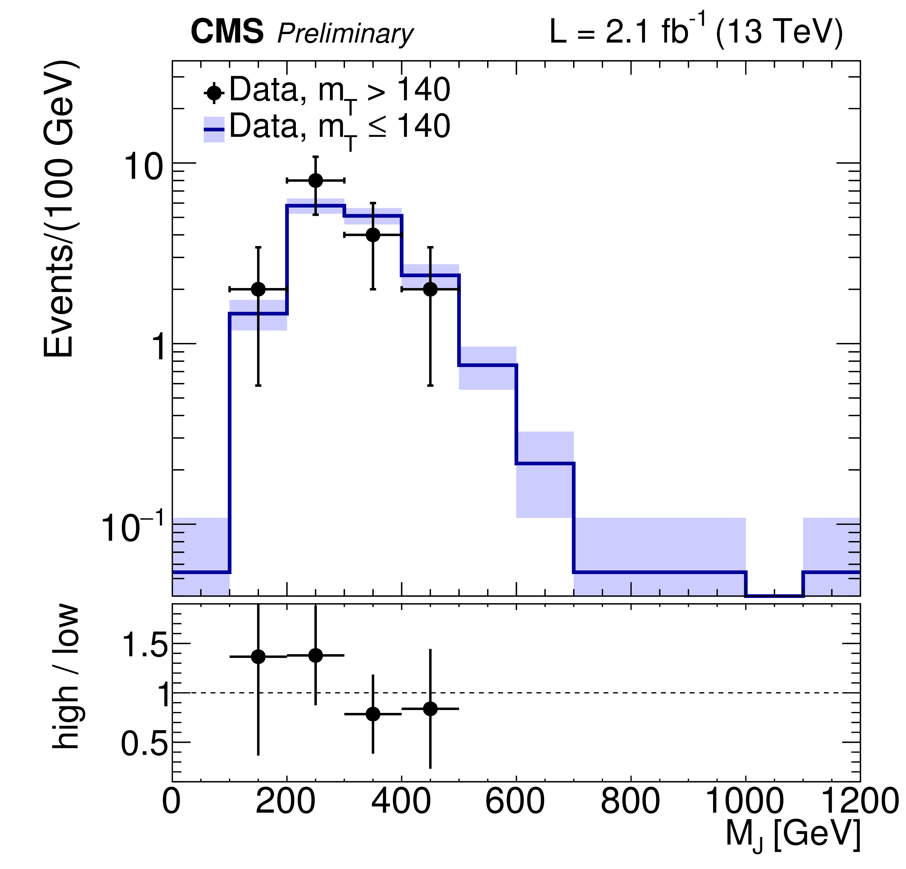
png ; pdf ;	Figure 14-c: Distributions of ${M_J}$ for events with ${N_{\text {b}}} =$ 1 in data and simulated event samples (MC). a,b: ${M_J}$ distributions for ${m_{\mathrm {T}}} \leq$ 140 GeV (a) and ${m_{\mathrm {T}}} >$ 140 GeV (b). The overall MC event yields are normalized to that in the data. c: comparison of the ${M_J}$ distributions for low and high ${m_{\mathrm {T}}}$ in data, the former normalized to the number of events in the latter. The uncertainties on the ratio plots include the uncertainties from the numerator and denominator added in quadrature.
png ; pdf ;	Figure 15-a: Distributions of ${m_{\mathrm {T}}}$ for events with ${N_{\text {b}}} \geq$ 2 in data and simulated event samples. a,b: ${m_{\mathrm {T}}}$ distributions for 250 $< {M_J} \leq$ 400 GeV (a) and ${M_J} >$ 400 GeV (b). The overall MC event yields are normalized to that in the data. c: comparison of the ${m_{\mathrm {T}}}$ distributions for low and high ${M_J}$ in data, the former normalized to the number of events in the latter. The uncertainties on the ratio plots include the uncertainties from the numerator and denominator added in quadrature.
png ; pdf ;	Figure 15-b: Distributions of ${m_{\mathrm {T}}}$ for events with ${N_{\text {b}}} \geq$ 2 in data and simulated event samples. a,b: ${m_{\mathrm {T}}}$ distributions for 250 $< {M_J} \leq$ 400 GeV (a) and ${M_J} >$ 400 GeV (b). The overall MC event yields are normalized to that in the data. c: comparison of the ${m_{\mathrm {T}}}$ distributions for low and high ${M_J}$ in data, the former normalized to the number of events in the latter. The uncertainties on the ratio plots include the uncertainties from the numerator and denominator added in quadrature.
png ; pdf ;	Figure 15-c: Distributions of ${m_{\mathrm {T}}}$ for events with ${N_{\text {b}}} \geq$ 2 in data and simulated event samples. a,b: ${m_{\mathrm {T}}}$ distributions for 250 $< {M_J} \leq$ 400 GeV (a) and ${M_J} >$ 400 GeV (b). The overall MC event yields are normalized to that in the data. c: comparison of the ${m_{\mathrm {T}}}$ distributions for low and high ${M_J}$ in data, the former normalized to the number of events in the latter. The uncertainties on the ratio plots include the uncertainties from the numerator and denominator added in quadrature.
png ; pdf ;	Figure 16-a: Distributions of ${M_J}$ for events with ${N_{\text {b}}} \geq$ 2. a,b: ${M_J}$ distributions for ${m_{\mathrm {T}}} \leq$ 140 GeV (a) and ${m_{\mathrm {T}}} >$ 140 GeV (b). The overall MC event yields are normalized to that in the data Bottom: comparison of the ${M_J}$ distributions for low and high ${m_{\mathrm {T}}}$ in data, the former normalized to the number of events in the latter. The uncertainties on the ratio plots include the uncertainties from the numerator and denominator added in quadrature.
png ; pdf ;	Figure 16-b: Distributions of ${M_J}$ for events with ${N_{\text {b}}} \geq$ 2. a,b: ${M_J}$ distributions for ${m_{\mathrm {T}}} \leq$ 140 GeV (a) and ${m_{\mathrm {T}}} >$ 140 GeV (b). The overall MC event yields are normalized to that in the data Bottom: comparison of the ${M_J}$ distributions for low and high ${m_{\mathrm {T}}}$ in data, the former normalized to the number of events in the latter. The uncertainties on the ratio plots include the uncertainties from the numerator and denominator added in quadrature.
png ; pdf ;	Figure 16-c: Distributions of ${M_J}$ for events with ${N_{\text {b}}} \geq$ 2. a,b: ${M_J}$ distributions for ${m_{\mathrm {T}}} \leq$ 140 GeV (a) and ${m_{\mathrm {T}}} >$ 140 GeV (b). The overall MC event yields are normalized to that in the data Bottom: comparison of the ${M_J}$ distributions for low and high ${m_{\mathrm {T}}}$ in data, the former normalized to the number of events in the latter. The uncertainties on the ratio plots include the uncertainties from the numerator and denominator added in quadrature.
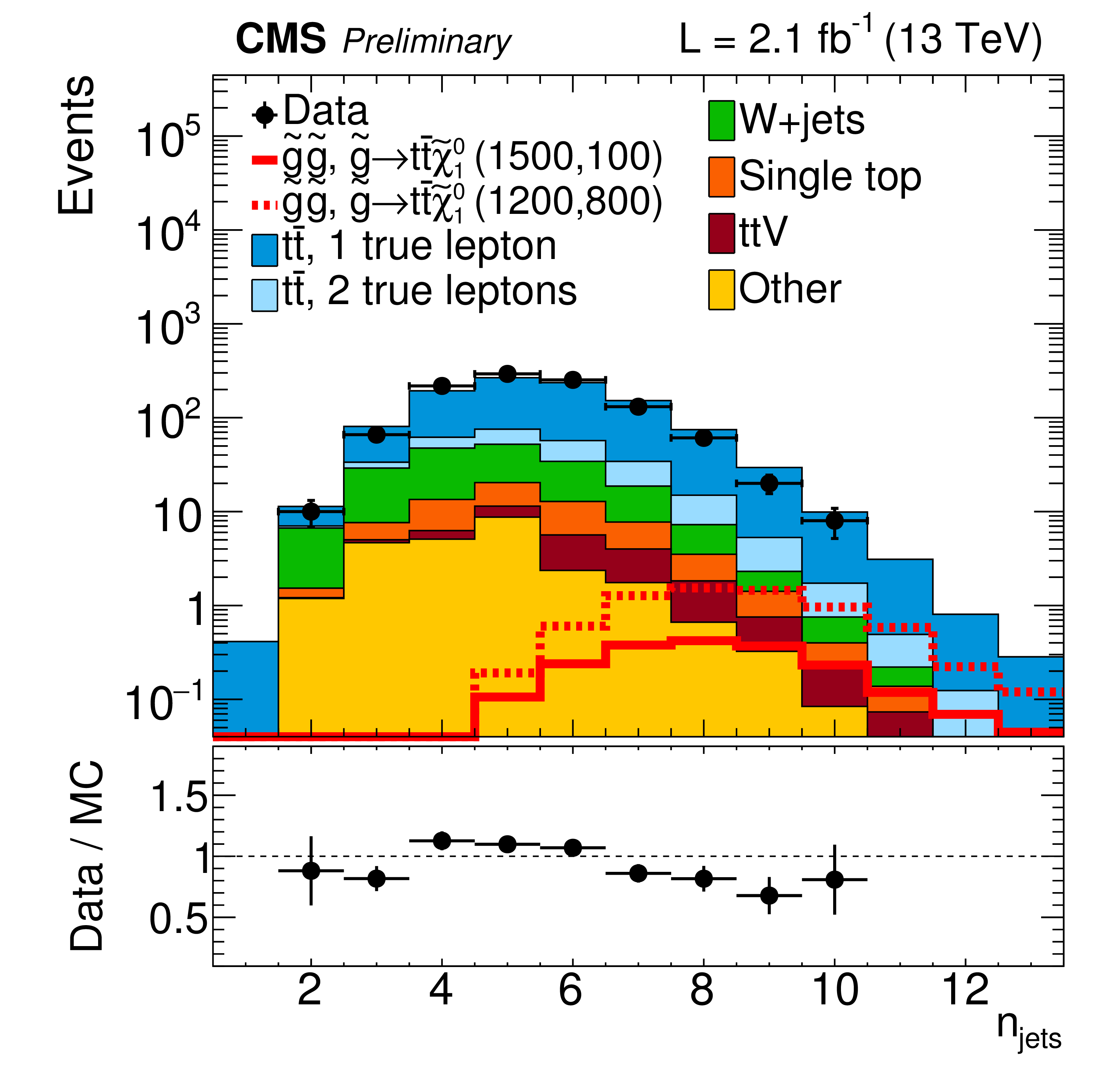
png ; pdf ;	Figure 17-a: Distributions ${E_{\mathrm {T}}^{\text {miss}}}$ and ${N_{\text {jets}}}$ for events with ${N_{\text {b}}} \geq$ 1 in data and simulated event samples. Distributions of ${E_{\mathrm {T}}^{\text {miss}}}$ (a,c) and ${N_{\text {jets}}}$ (b,d), for ${m_{\mathrm {T}}} \leq$ 140 GeV (c,d) and ${m_{\mathrm {T}}} >$ 140 GeV (a,b). The overall MC event yields are normalized to that in the data, with the normalization factor given below the legend.
png ; pdf ;	Figure 17-b: Distributions ${E_{\mathrm {T}}^{\text {miss}}}$ and ${N_{\text {jets}}}$ for events with ${N_{\text {b}}} \geq$ 1 in data and simulated event samples. Distributions of ${E_{\mathrm {T}}^{\text {miss}}}$ (a,c) and ${N_{\text {jets}}}$ (b,d), for ${m_{\mathrm {T}}} \leq$ 140 GeV (c,d) and ${m_{\mathrm {T}}} >$ 140 GeV (a,b). The overall MC event yields are normalized to that in the data, with the normalization factor given below the legend.
png ; pdf ;	Figure 17-c: Distributions ${E_{\mathrm {T}}^{\text {miss}}}$ and ${N_{\text {jets}}}$ for events with ${N_{\text {b}}} \geq$ 1 in data and simulated event samples. Distributions of ${E_{\mathrm {T}}^{\text {miss}}}$ (a,c) and ${N_{\text {jets}}}$ (b,d), for ${m_{\mathrm {T}}} \leq$ 140 GeV (c,d) and ${m_{\mathrm {T}}} >$ 140 GeV (a,b). The overall MC event yields are normalized to that in the data, with the normalization factor given below the legend.
png ; pdf ;	Figure 17-d: Distributions ${E_{\mathrm {T}}^{\text {miss}}}$ and ${N_{\text {jets}}}$ for events with ${N_{\text {b}}} \geq$ 1 in data and simulated event samples. Distributions of ${E_{\mathrm {T}}^{\text {miss}}}$ (a,c) and ${N_{\text {jets}}}$ (b,d), for ${m_{\mathrm {T}}} \leq$ 140 GeV (c,d) and ${m_{\mathrm {T}}} >$ 140 GeV (a,b). The overall MC event yields are normalized to that in the data, with the normalization factor given below the legend.
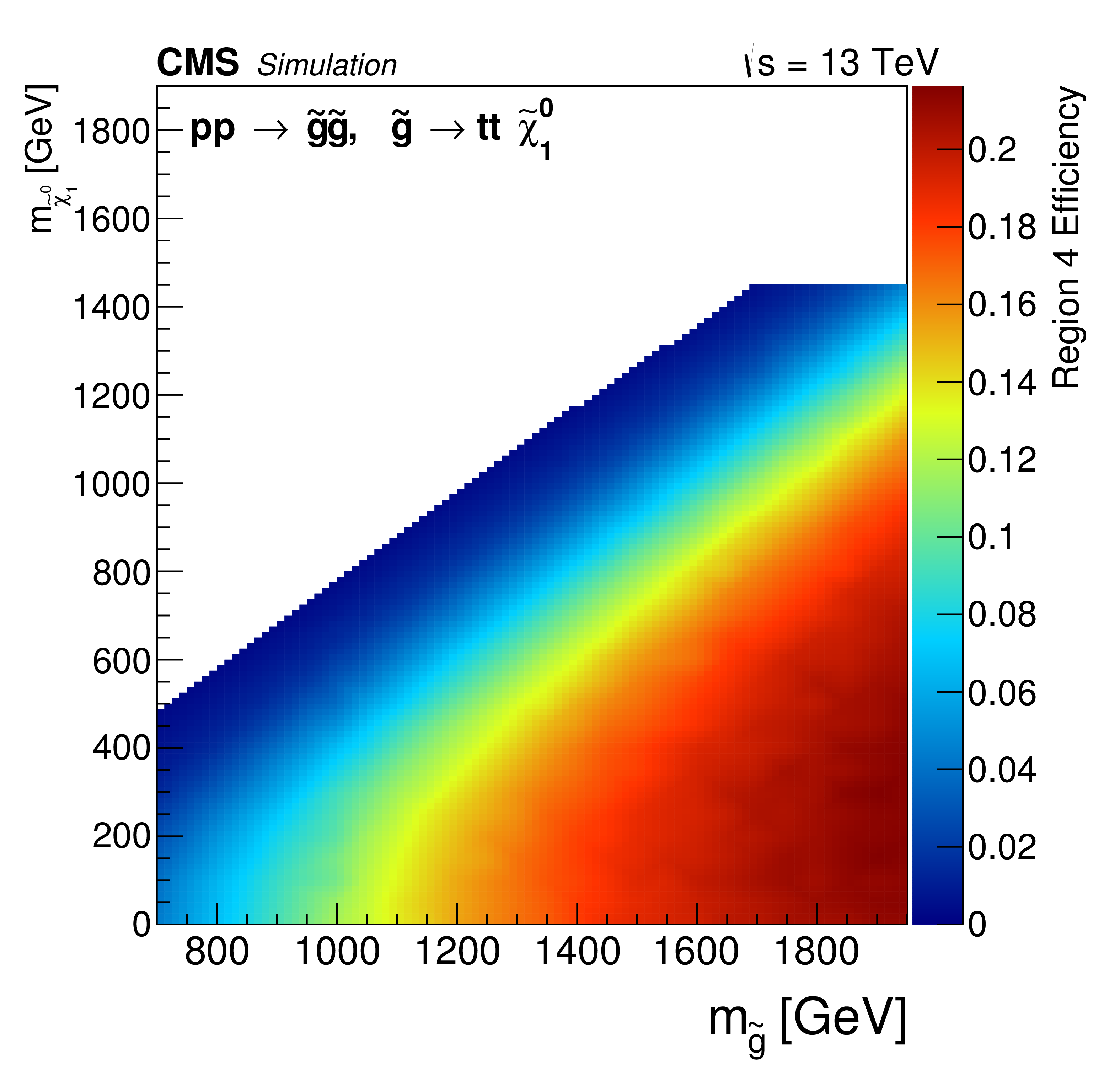
png ; pdf ;	Figure 18-a: Region 4 signal efficiency (a) and yields normalized to 2.1 fb $^{-1}$ (b) in the $m_{\mathrm{q} } - m_{ {\tilde{\chi }^0_1} }$ plane.
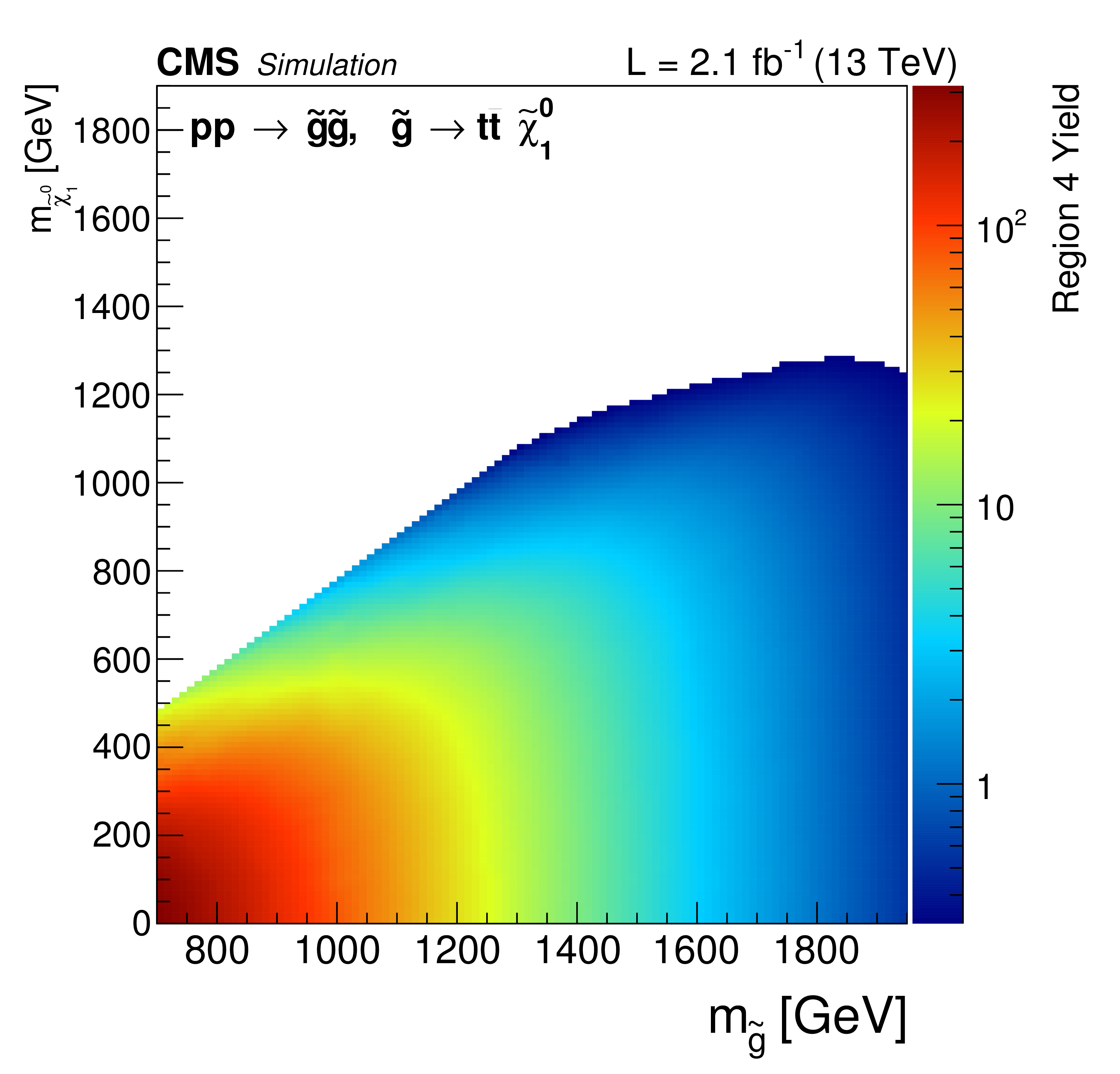
png ; pdf ;	Figure 18-b: Region 4 signal efficiency (a) and yields normalized to 2.1 fb $^{-1}$ (b) in the $m_{\mathrm{q} } - m_{ {\tilde{\chi }^0_1} }$ plane.
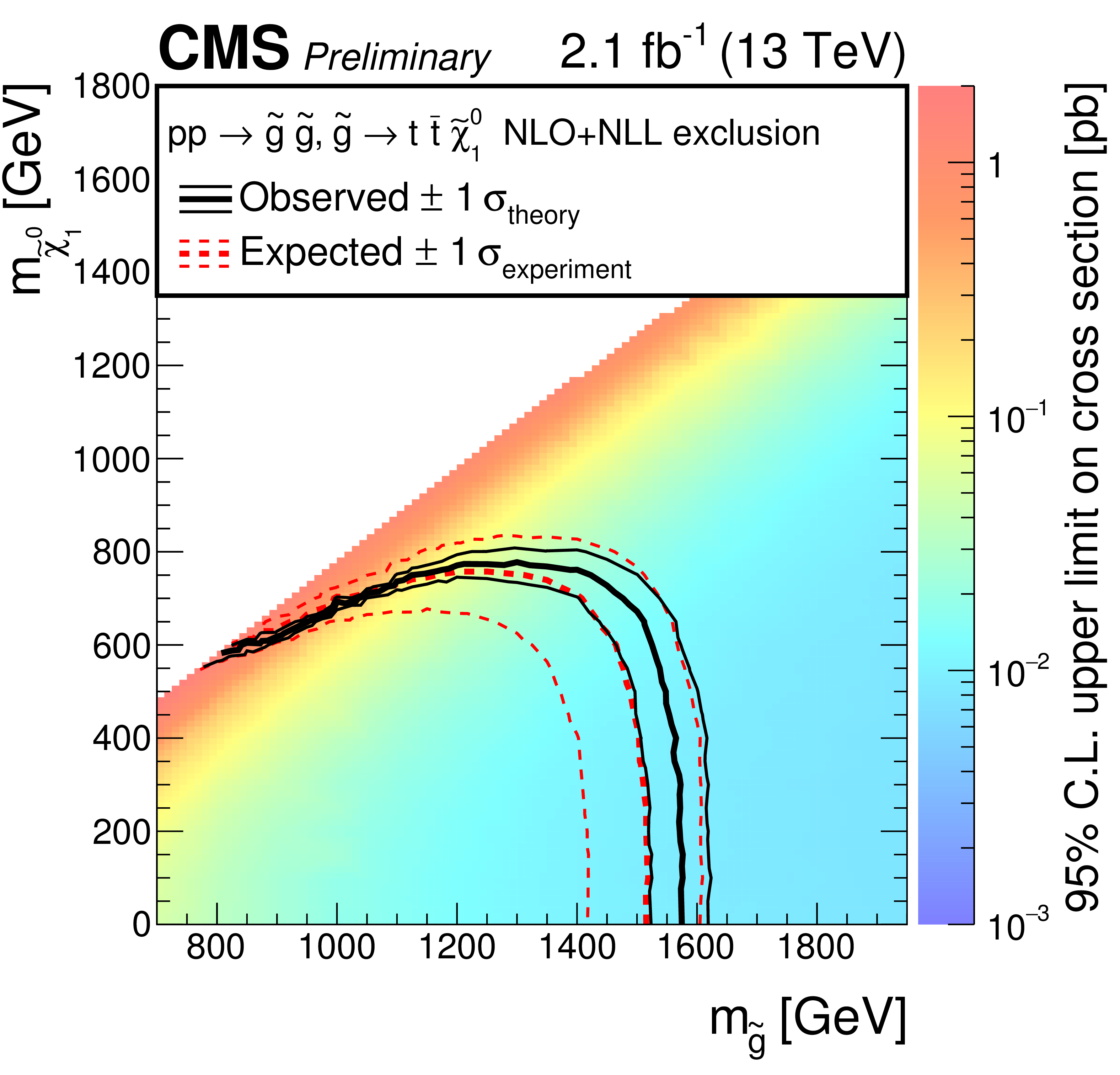
png ; pdf ;	Figure 19: The 95% confidence level upper limits on the production cross section for the $\mathrm{ pp \rightarrow \tilde{g} \tilde{g} }$ , $\mathrm{ \tilde{g} \rightarrow t \bar{t} \tilde{\chi }^0_1 }$ in the $m_{ \mathrm{ \tilde{g} } } - m_{ \tilde{\chi }^0_1 }$ plane.

Compact Muon Solenoid
LHC, CERN