

Compact Muon Solenoid
LHC, CERN
| CMS-PAS-SUS-15-004 | ||
| Inclusive search for supersymmetry using the razor variables at $\sqrt{s} =$ 13 TeV | ||
| CMS Collaboration | ||
| December 2015 | ||
| Abstract: An inclusive search for supersymmetry with the razor variables is performed using a data sample of proton-proton collisions corresponding to an integrated luminosity of 2.1 fb$^{-1}$ collected with the CMS experiment at a center-of-mass energy of $\sqrt{s} =$ 13 TeV. The search covers events with zero or one lepton, and four or more jets in the final state. No significant excess over the background prediction is observed in data, and 95\% confidence level exclusion limits are placed on the masses of new heavy particles in a variety of simplified models. Assuming the neutralino is the lightest supersymmetric particle with a mass of 100 GeV and the gluino decays to a neutralino and a bottom quark-antiquark pair, the pair production of gluinos is excluded for gluino masses up to 1650 GeV. For the corresponding decays to top quarks and first or second generation quarks, gluinos with masses up to 1600 GeV and 1350 GeV are excluded, respectively. | ||
|
Links:
CDS record (PDF) ;
CADI line (restricted) ;
These preliminary results are superseded in this paper, PRD 95 (2017) 012003. The superseded preliminary plots can be found here. |
||
| Figures | |
png ; pdf ; |
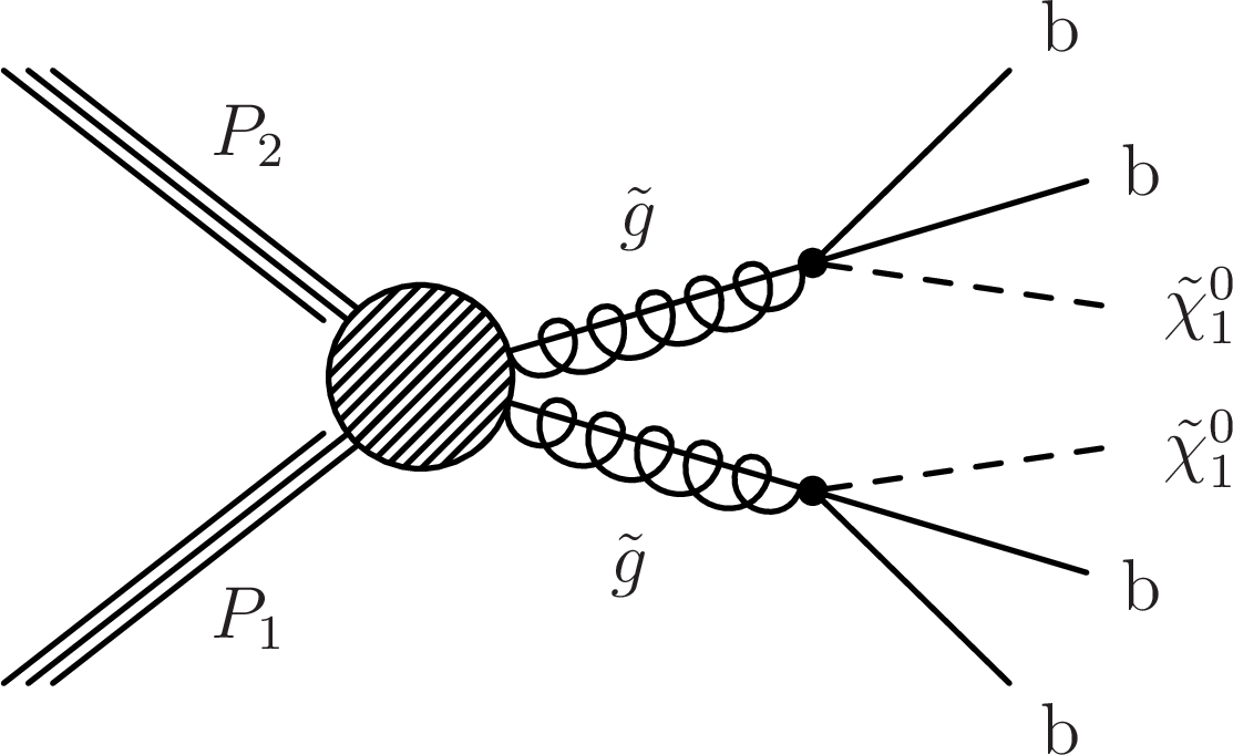
Figure 1-a:
Diagrams displaying the event topologies of gluino pair production considered in this analysis. |
png ; pdf ; |
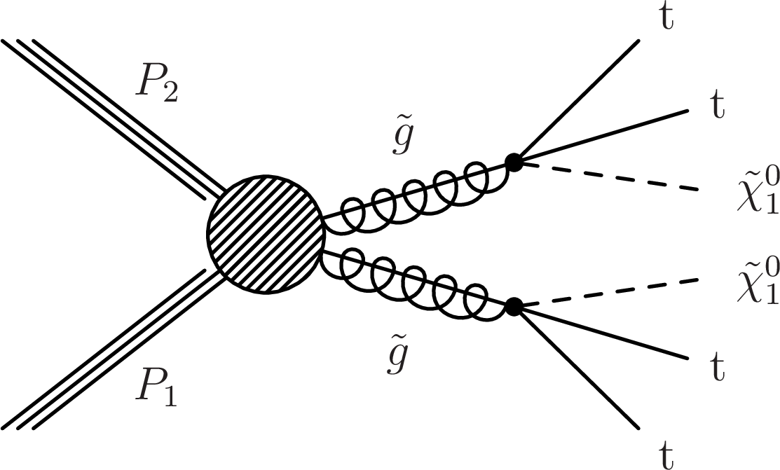
Figure 1-b:
Diagrams displaying the event topologies of gluino pair production considered in this analysis. |
png ; pdf ; |
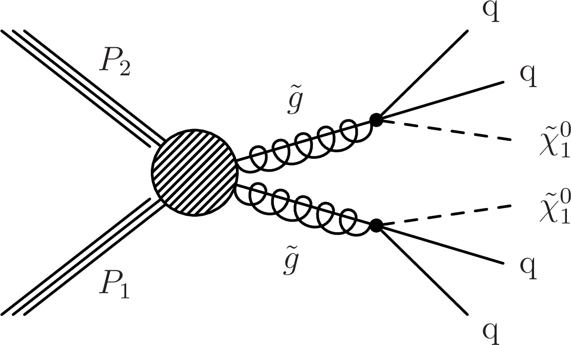
Figure 1-c:
Diagrams displaying the event topologies of gluino pair production considered in this analysis. |

png ; pdf ; |
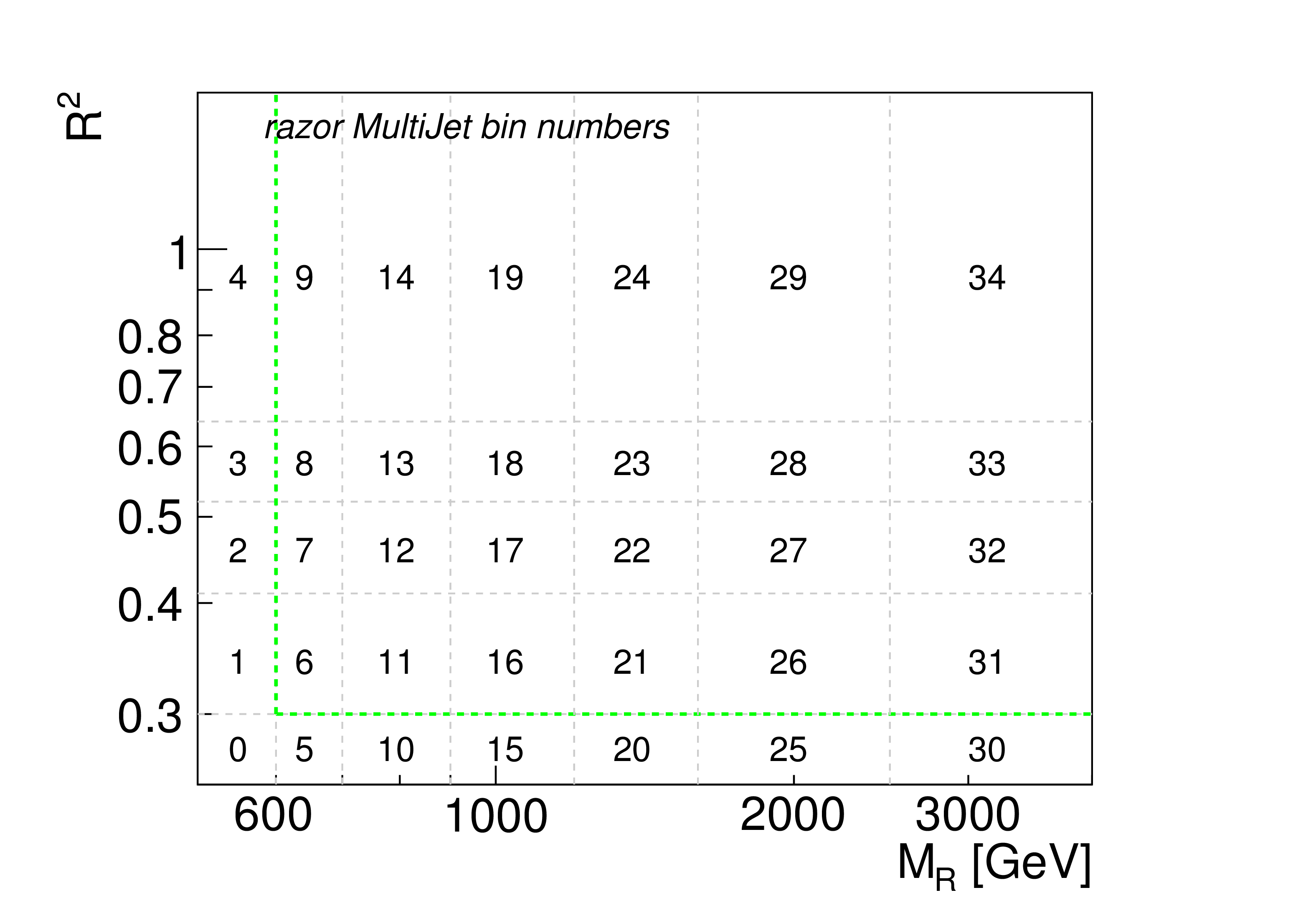
Figure 2-a:
Definition of the sideband and the signal-sensitive regions used in the analysis, for (a) the zero lepton category and (b) the one lepton categories. Definition of the bin numbers associated to each region in the $R^2$-$M_R$ plane for (c) the zero lepton category and (d) the one lepton categories. |
png ; pdf ; |
Figure 2-b:
Definition of the sideband and the signal-sensitive regions used in the analysis, for (a) the zero lepton category and (b) the one lepton categories. Definition of the bin numbers associated to each region in the $R^2$-$M_R$ plane for (c) the zero lepton category and (d) the one lepton categories. |
png ; pdf ; |
Figure 2-c:
Definition of the sideband and the signal-sensitive regions used in the analysis, for (a) the zero lepton category and (b) the one lepton categories. Definition of the bin numbers associated to each region in the $R^2$-$M_R$ plane for (c) the zero lepton category and (d) the one lepton categories. |
png ; pdf ; |
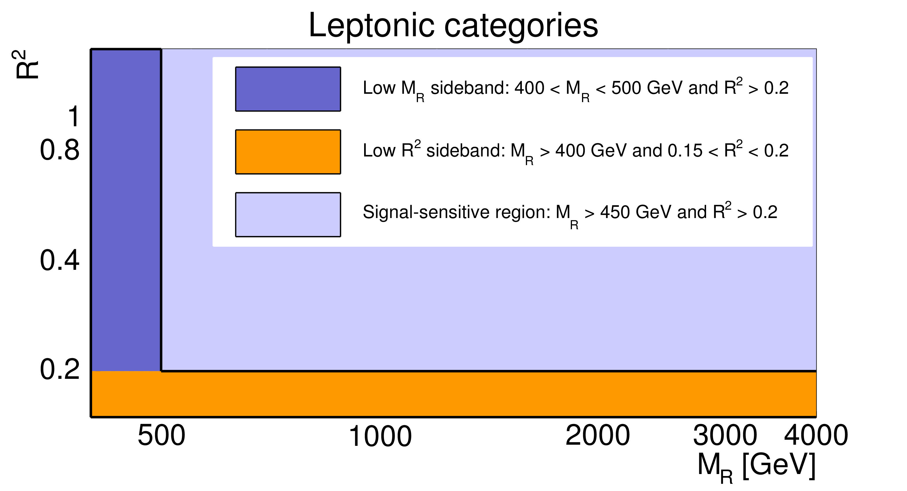
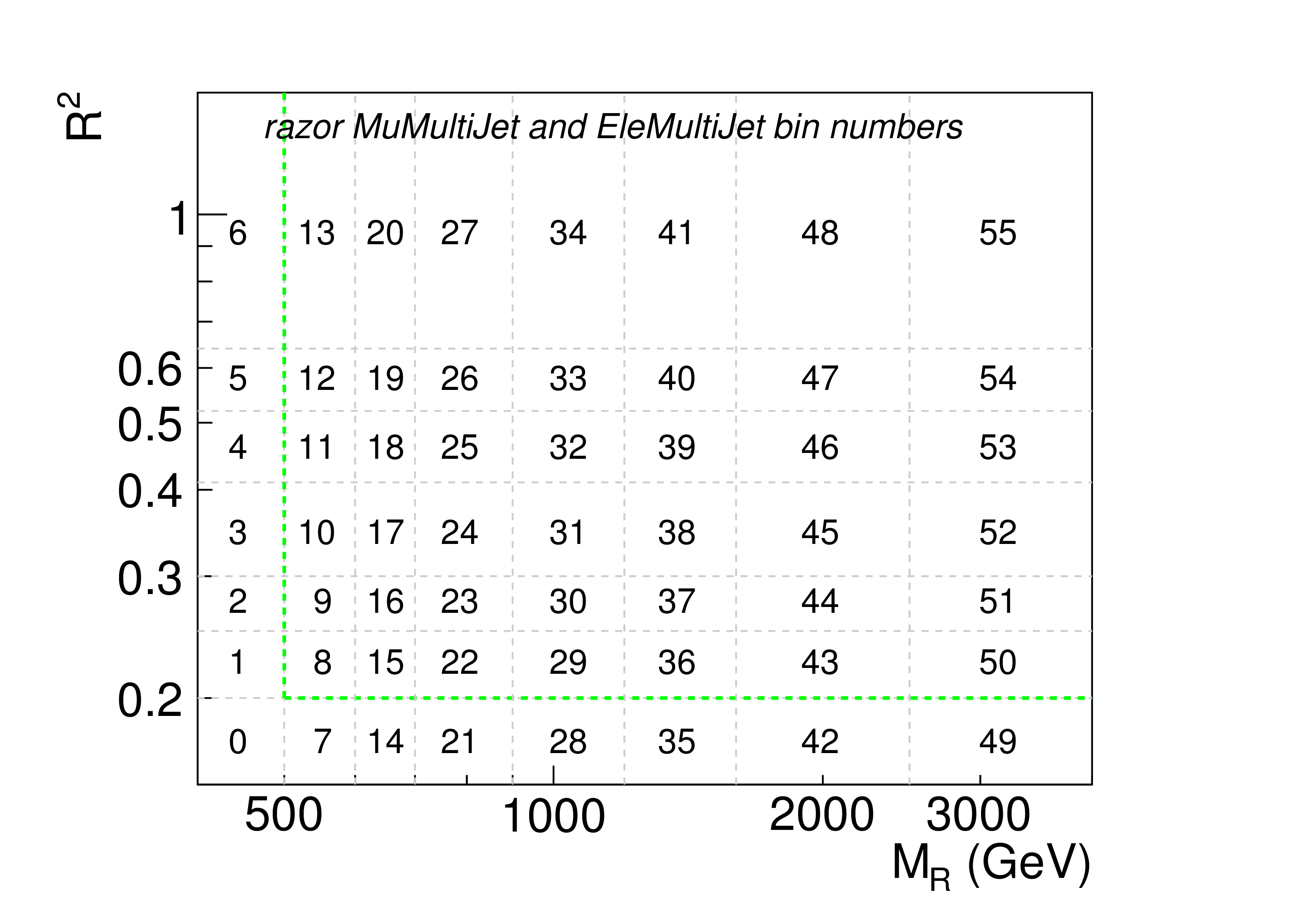
Figure 2-d:
Definition of the sideband and the signal-sensitive regions used in the analysis, for (a) the zero lepton category and (b) the one lepton categories. Definition of the bin numbers associated to each region in the $R^2$-$M_R$ plane for (c) the zero lepton category and (d) the one lepton categories. |
png ; pdf ; |
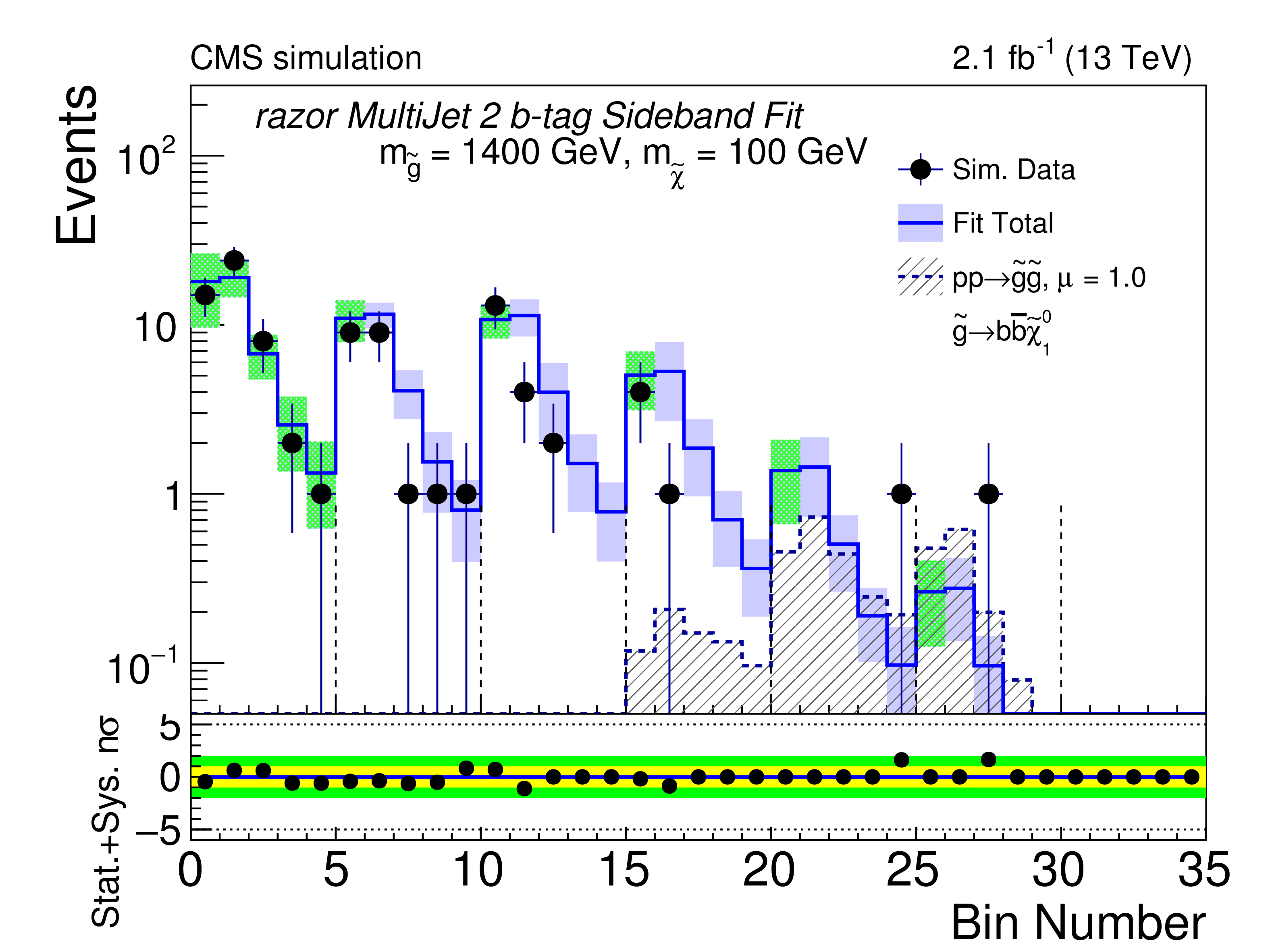
Figure 3-a:
The result of the background-only fit performed in the sideband on a signal-plus-background toy dataset using gluino pair-production simplified models signals, where gluinos decay with a 100% branching fraction to a $ \mathrm{ t \bar{t} } $ pair and the LSP, with $m_{\tilde{g}} = $ 1400 GeV and $m_{\tilde{\chi }}=$ 100 GeV, at nominal signal strength. One-dimensional representations of the fit result for the 2 b-tag (top left) and $\geq 3$ b-tag categories (bottom left) are shown on the left, where the uncertainty band for the sideband bins are shown in green. Vertical dashed lines denote the boundaries of different $M_R$ bins, as defined in Fig. 2. The distributions of deviations in the $R^2$-$M_R$ plane, expressed in units of standard deviations, are shown on the right for the 2 b-tag (top right) and $\geq 3$ b-tag categories (bottom right). Statistical and systematic uncertainties are both considered in the calculation of the deviations. |
png ; pdf ; |
Figure 3-b:
The result of the background-only fit performed in the sideband on a signal-plus-background toy dataset using gluino pair-production simplified models signals, where gluinos decay with a 100% branching fraction to a $ \mathrm{ t \bar{t} } $ pair and the LSP, with $m_{\tilde{g}} = $ 1400 GeV and $m_{\tilde{\chi }}=$ 100 GeV, at nominal signal strength. One-dimensional representations of the fit result for the 2 b-tag (top left) and $\geq 3$ b-tag categories (bottom left) are shown on the left, where the uncertainty band for the sideband bins are shown in green. Vertical dashed lines denote the boundaries of different $M_R$ bins, as defined in Fig. 2. The distributions of deviations in the $R^2$-$M_R$ plane, expressed in units of standard deviations, are shown on the right for the 2 b-tag (top right) and $\geq 3$ b-tag categories (bottom right). Statistical and systematic uncertainties are both considered in the calculation of the deviations. |

png ; pdf ; |
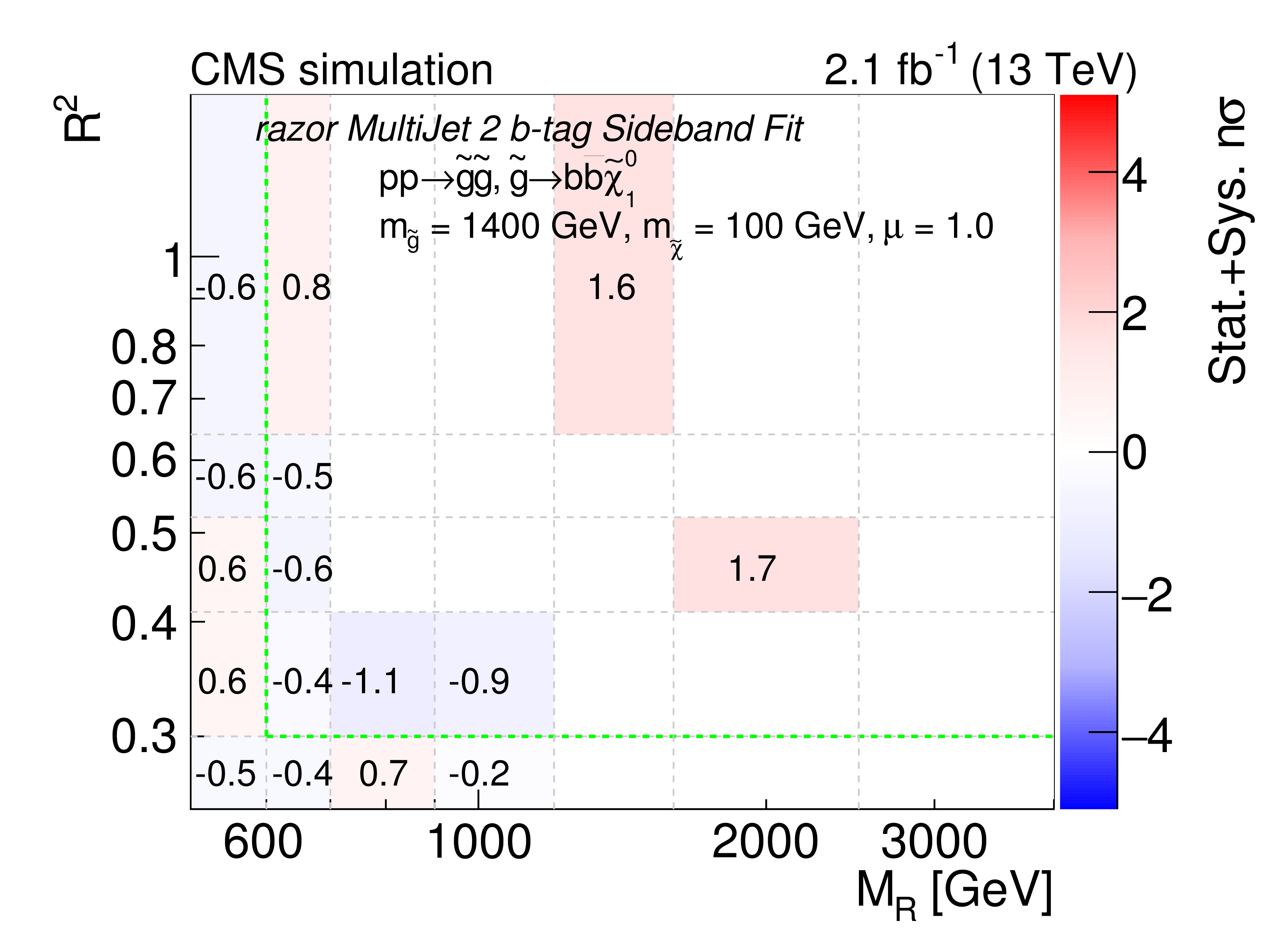
Figure 3-c:
The result of the background-only fit performed in the sideband on a signal-plus-background toy dataset using gluino pair-production simplified models signals, where gluinos decay with a 100% branching fraction to a $ \mathrm{ t \bar{t} } $ pair and the LSP, with $m_{\tilde{g}} = $ 1400 GeV and $m_{\tilde{\chi }}=$ 100 GeV, at nominal signal strength. One-dimensional representations of the fit result for the 2 b-tag (top left) and $\geq 3$ b-tag categories (bottom left) are shown on the left, where the uncertainty band for the sideband bins are shown in green. Vertical dashed lines denote the boundaries of different $M_R$ bins, as defined in Fig. 2. The distributions of deviations in the $R^2$-$M_R$ plane, expressed in units of standard deviations, are shown on the right for the 2 b-tag (top right) and $\geq 3$ b-tag categories (bottom right). Statistical and systematic uncertainties are both considered in the calculation of the deviations. |
png ; pdf ; |
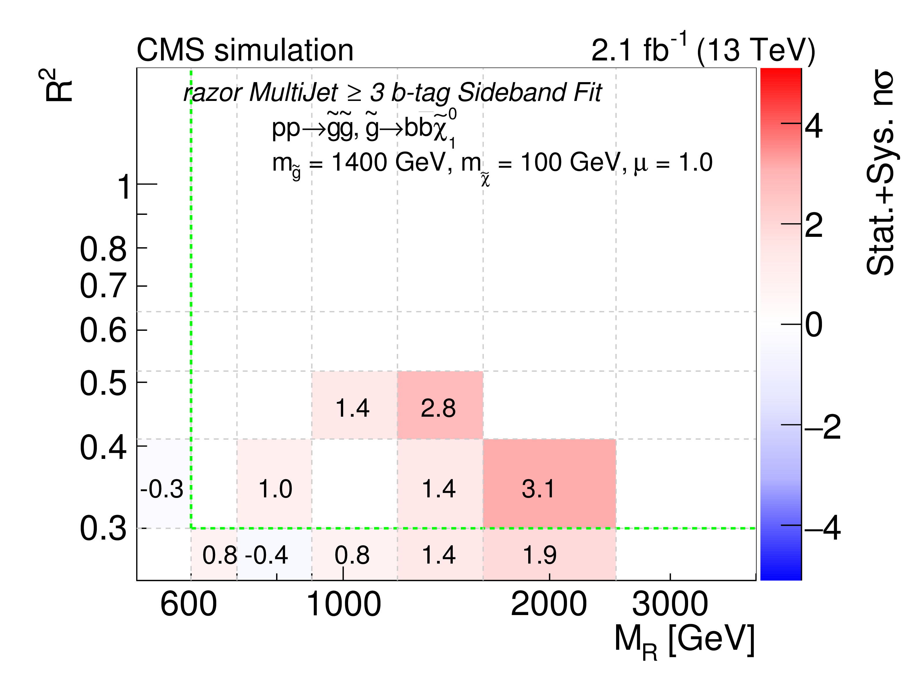
Figure 3-d:
The result of the background-only fit performed in the sideband on a signal-plus-background toy dataset using gluino pair-production simplified models signals, where gluinos decay with a 100% branching fraction to a $ \mathrm{ t \bar{t} } $ pair and the LSP, with $m_{\tilde{g}} = $ 1400 GeV and $m_{\tilde{\chi }}=$ 100 GeV, at nominal signal strength. One-dimensional representations of the fit result for the 2 b-tag (top left) and $\geq 3$ b-tag categories (bottom left) are shown on the left, where the uncertainty band for the sideband bins are shown in green. Vertical dashed lines denote the boundaries of different $M_R$ bins, as defined in Fig. 2. The distributions of deviations in the $R^2$-$M_R$ plane, expressed in units of standard deviations, are shown on the right for the 2 b-tag (top right) and $\geq 3$ b-tag categories (bottom right). Statistical and systematic uncertainties are both considered in the calculation of the deviations. |

png ; pdf ; |
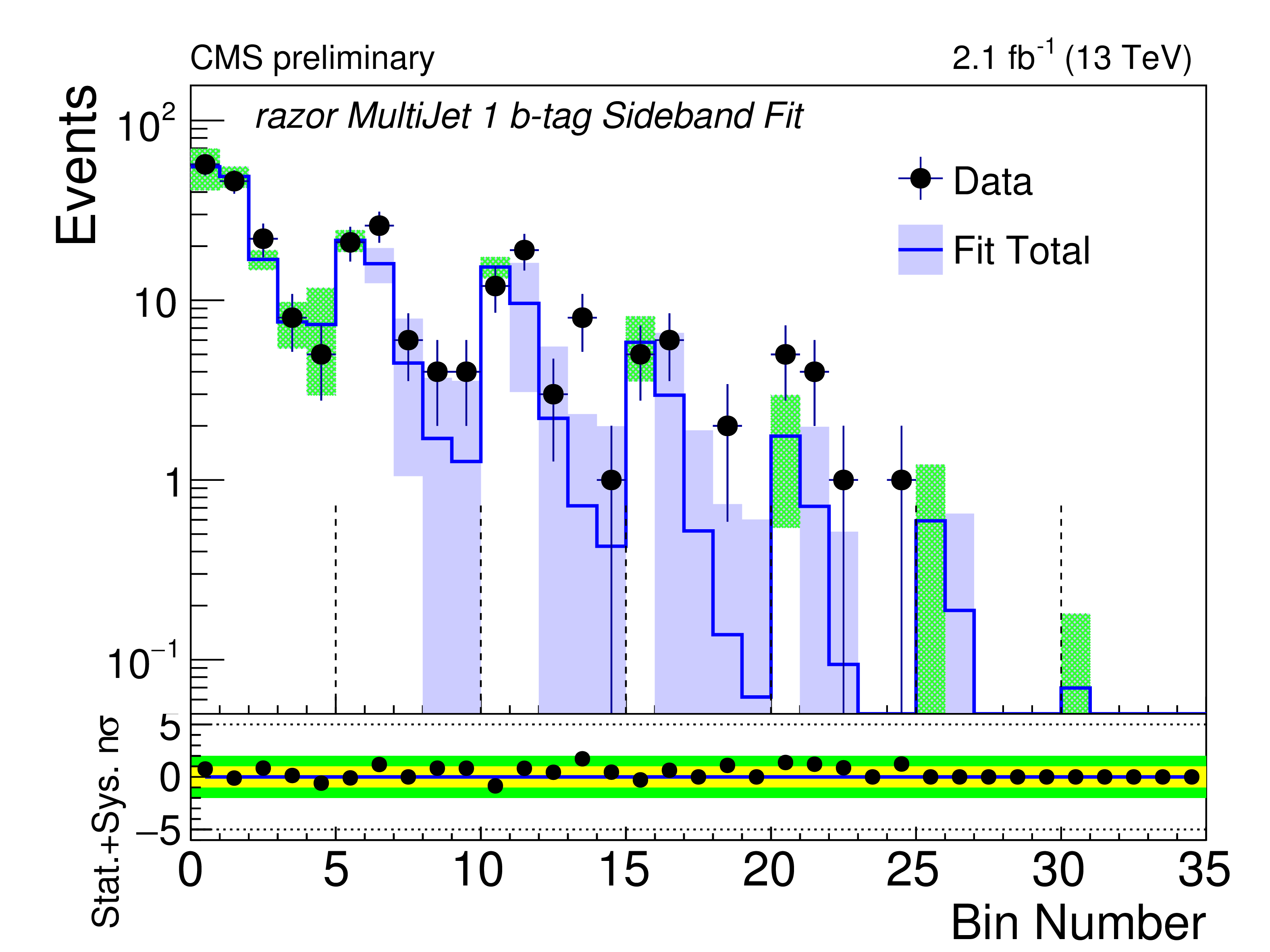
Figure 4-a:
Comparison of the predicted background with the observed data in bins of $M_R$ and $R^2$ variables in the Multijet category. The colored bands represents the systematic uncertainties in the background prediction. The uncertainty bands for the sideband bins are shown in green. On the bottom inset, the deviation between the observed data and the background prediction are plotted in units of standard deviation, taking into account both statistical and systematic uncertainties. Vertical dashed lines denote the boundaries of different $M_R$ bins, as defined in Figure 2. |
png ; pdf ; |
Figure 4-b:
Comparison of the predicted background with the observed data in bins of $M_R$ and $R^2$ variables in the Multijet category. The colored bands represents the systematic uncertainties in the background prediction. The uncertainty bands for the sideband bins are shown in green. On the bottom inset, the deviation between the observed data and the background prediction are plotted in units of standard deviation, taking into account both statistical and systematic uncertainties. Vertical dashed lines denote the boundaries of different $M_R$ bins, as defined in Figure 2. |

png ; pdf ; |
Figure 4-c:
Comparison of the predicted background with the observed data in bins of $M_R$ and $R^2$ variables in the Multijet category. The colored bands represents the systematic uncertainties in the background prediction. The uncertainty bands for the sideband bins are shown in green. On the bottom inset, the deviation between the observed data and the background prediction are plotted in units of standard deviation, taking into account both statistical and systematic uncertainties. Vertical dashed lines denote the boundaries of different $M_R$ bins, as defined in Figure 2. |

png ; pdf ; |
Figure 4-d:
Comparison of the predicted background with the observed data in bins of $M_R$ and $R^2$ variables in the Multijet category. The colored bands represents the systematic uncertainties in the background prediction. The uncertainty bands for the sideband bins are shown in green. On the bottom inset, the deviation between the observed data and the background prediction are plotted in units of standard deviation, taking into account both statistical and systematic uncertainties. Vertical dashed lines denote the boundaries of different $M_R$ bins, as defined in Figure 2. |
png ; pdf ; |
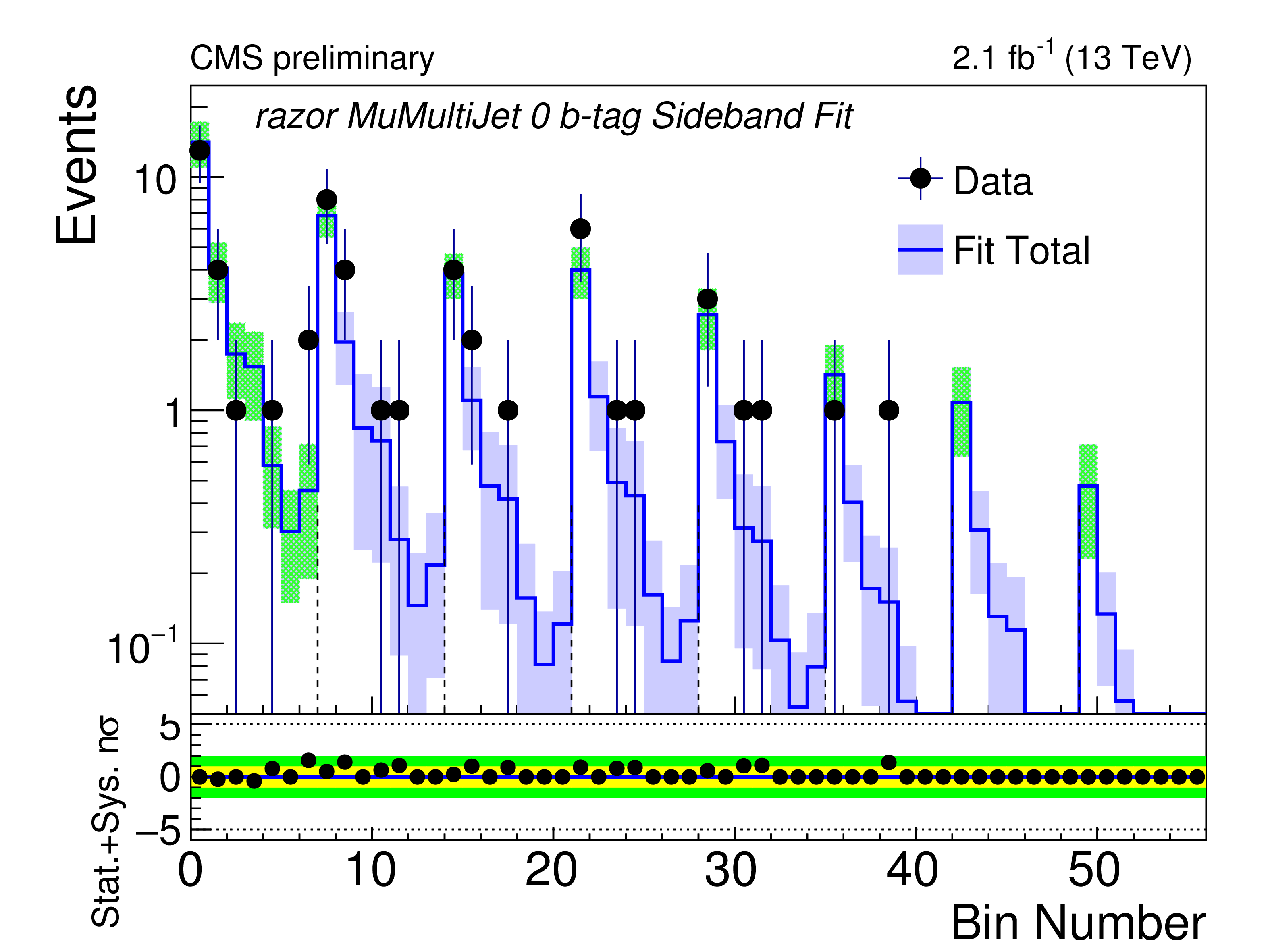
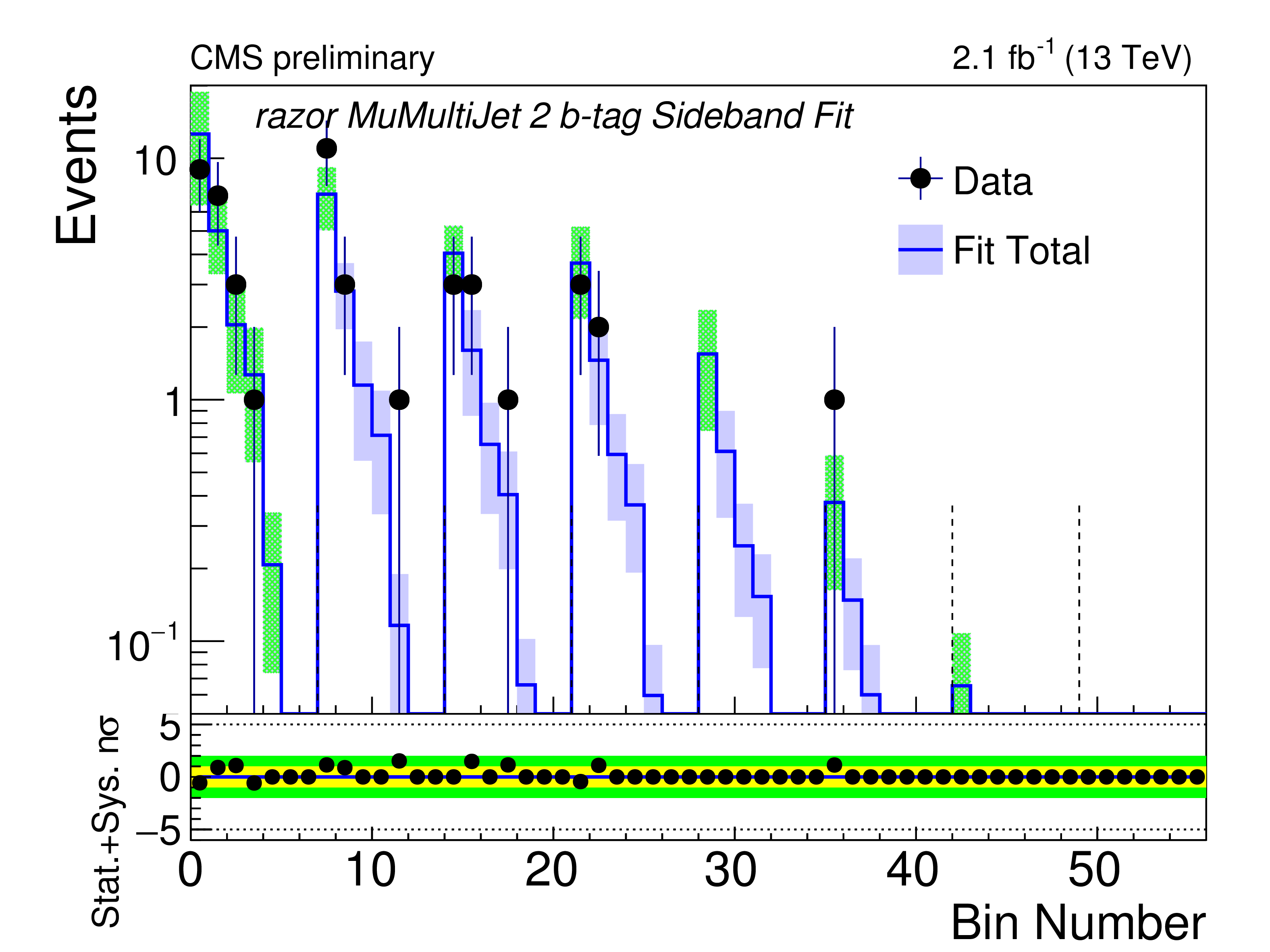
Figure 5-a:
Comparison of the predicted background with the observed data in bins of $M_R$ and $R^2$ variables in the Muon Multijet category. The colored bands represents the systematic uncertainties in the background prediction. The uncertainty bands for the sideband bins are shown in green. On the bottom inset, the deviation between the observed data and the background prediction are plotted in units of standard deviation, taking into account both statistical and systematic uncertainties. Vertical dashed lines denote the boundaries of different $M_R$ bins, as defined in Figure 2. |
png ; pdf ; |
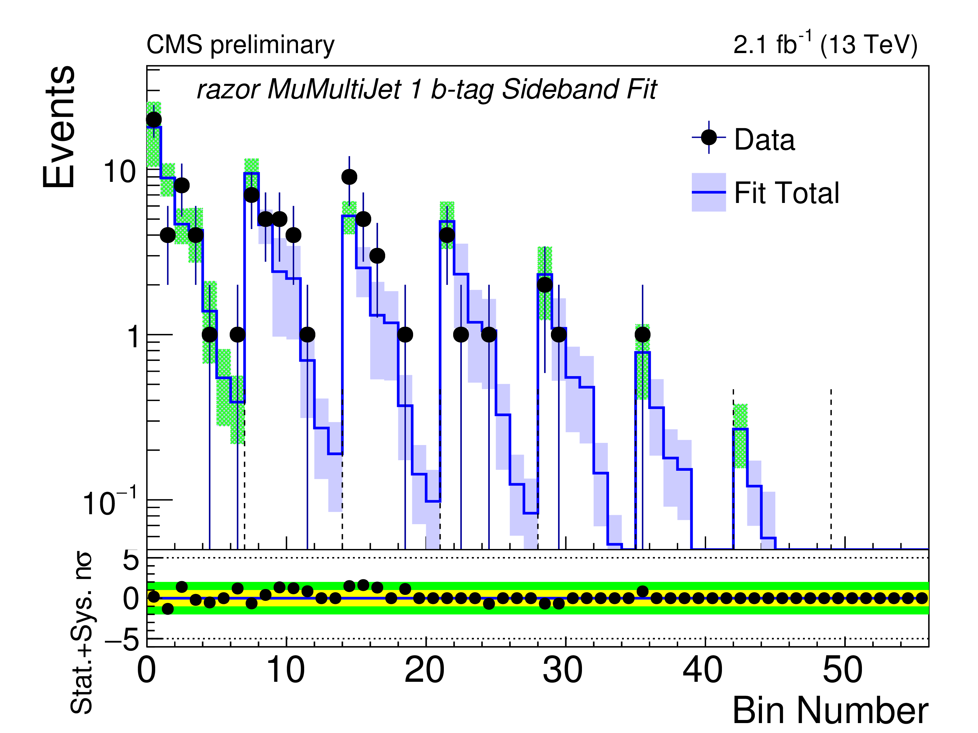
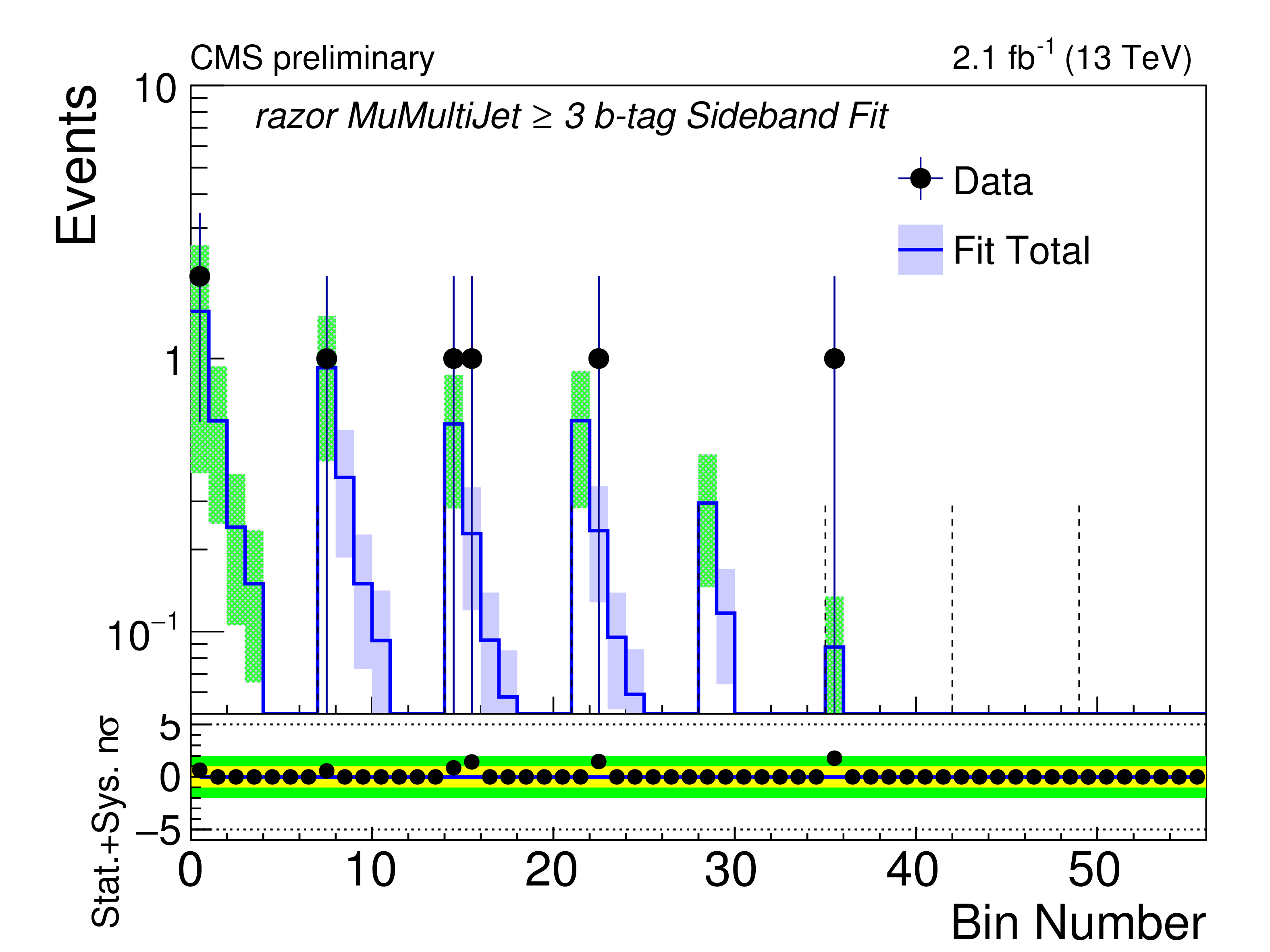
Figure 5-b:
Comparison of the predicted background with the observed data in bins of $M_R$ and $R^2$ variables in the Muon Multijet category. The colored bands represents the systematic uncertainties in the background prediction. The uncertainty bands for the sideband bins are shown in green. On the bottom inset, the deviation between the observed data and the background prediction are plotted in units of standard deviation, taking into account both statistical and systematic uncertainties. Vertical dashed lines denote the boundaries of different $M_R$ bins, as defined in Figure 2. |
png ; pdf ; |
Figure 5-c:
Comparison of the predicted background with the observed data in bins of $M_R$ and $R^2$ variables in the Muon Multijet category. The colored bands represents the systematic uncertainties in the background prediction. The uncertainty bands for the sideband bins are shown in green. On the bottom inset, the deviation between the observed data and the background prediction are plotted in units of standard deviation, taking into account both statistical and systematic uncertainties. Vertical dashed lines denote the boundaries of different $M_R$ bins, as defined in Figure 2. |
png ; pdf ; |
Figure 5-d:
Comparison of the predicted background with the observed data in bins of $M_R$ and $R^2$ variables in the Muon Multijet category. The colored bands represents the systematic uncertainties in the background prediction. The uncertainty bands for the sideband bins are shown in green. On the bottom inset, the deviation between the observed data and the background prediction are plotted in units of standard deviation, taking into account both statistical and systematic uncertainties. Vertical dashed lines denote the boundaries of different $M_R$ bins, as defined in Figure 2. |
png ; pdf ; |
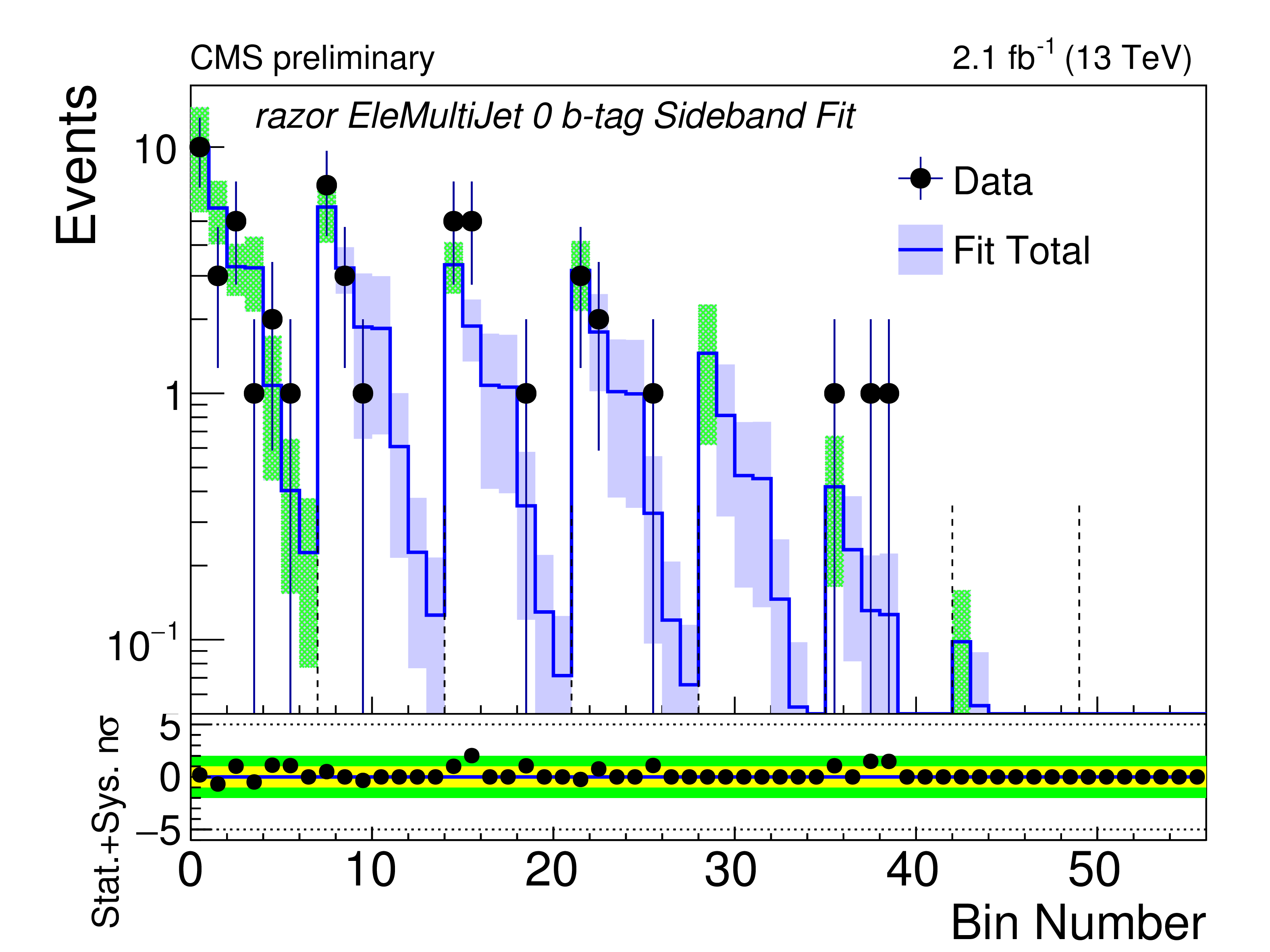
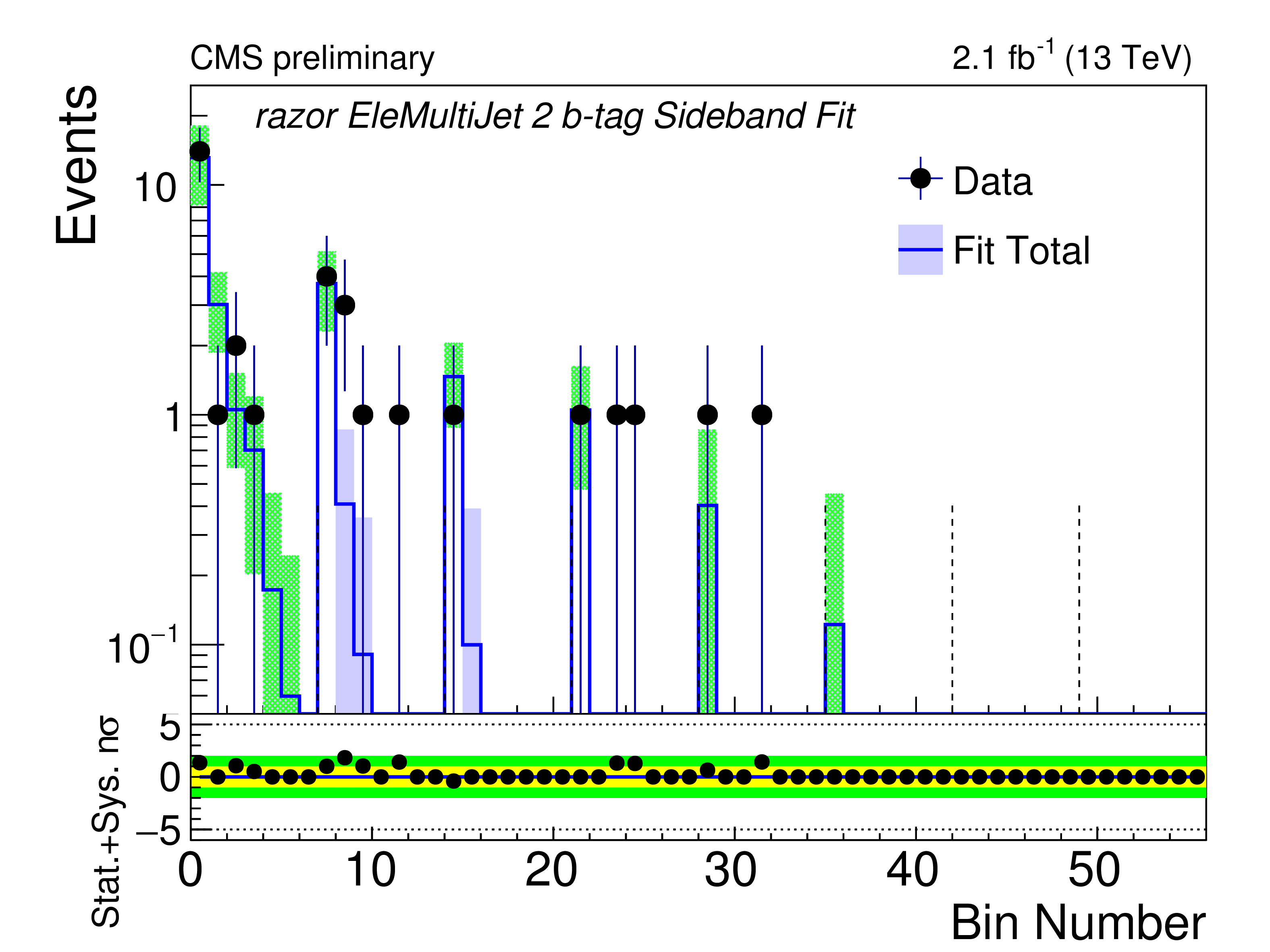
Figure 6-a:
Comparison of the predicted background with the observed data in bins of $M_R$ and $R^2$ variables in the Electron Multijet category. The colored bands represents the systematic uncertainties in the background prediction. The uncertainty bands for the sideband bins are shown in green. On the bottom inset, the deviation between the observed data and the background prediction are plotted in units of standard deviation, taking into account both statistical and systematic uncertainties. Vertical dashed lines denote the boundaries of different $M_R$ bins, as defined in Figure 2. |
png ; pdf ; |
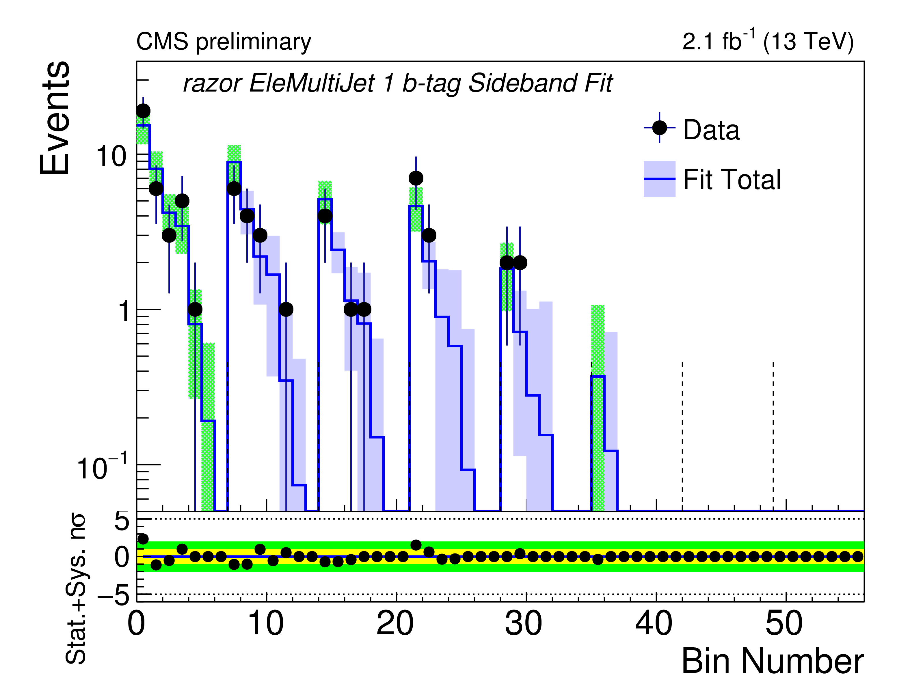
Figure 6-b:
Comparison of the predicted background with the observed data in bins of $M_R$ and $R^2$ variables in the Electron Multijet category. The colored bands represents the systematic uncertainties in the background prediction. The uncertainty bands for the sideband bins are shown in green. On the bottom inset, the deviation between the observed data and the background prediction are plotted in units of standard deviation, taking into account both statistical and systematic uncertainties. Vertical dashed lines denote the boundaries of different $M_R$ bins, as defined in Figure 2. |
png ; pdf ; |
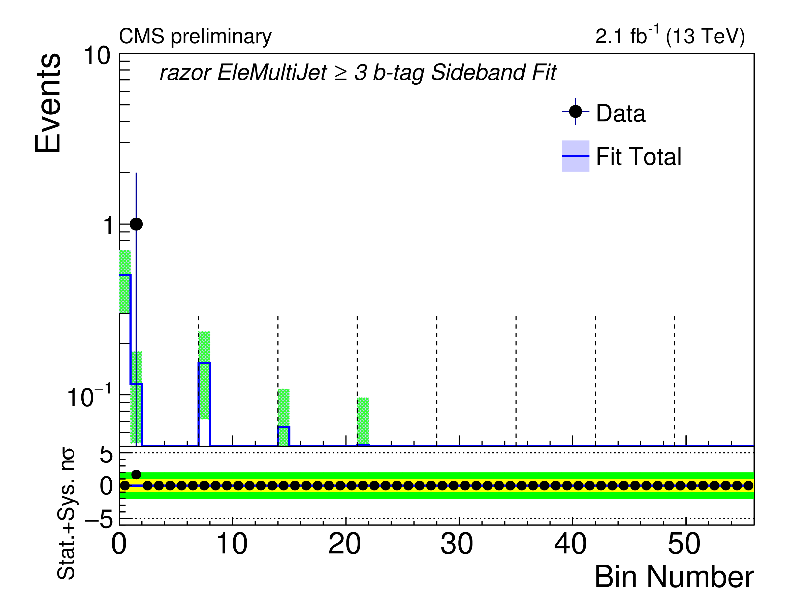
Figure 6-c:
Comparison of the predicted background with the observed data in bins of $M_R$ and $R^2$ variables in the Electron Multijet category. The colored bands represents the systematic uncertainties in the background prediction. The uncertainty bands for the sideband bins are shown in green. On the bottom inset, the deviation between the observed data and the background prediction are plotted in units of standard deviation, taking into account both statistical and systematic uncertainties. Vertical dashed lines denote the boundaries of different $M_R$ bins, as defined in Figure 2. |
png ; pdf ; |
Figure 6-d:
Comparison of the predicted background with the observed data in bins of $M_R$ and $R^2$ variables in the Electron Multijet category. The colored bands represents the systematic uncertainties in the background prediction. The uncertainty bands for the sideband bins are shown in green. On the bottom inset, the deviation between the observed data and the background prediction are plotted in units of standard deviation, taking into account both statistical and systematic uncertainties. Vertical dashed lines denote the boundaries of different $M_R$ bins, as defined in Figure 2. |
png ; pdf ; |
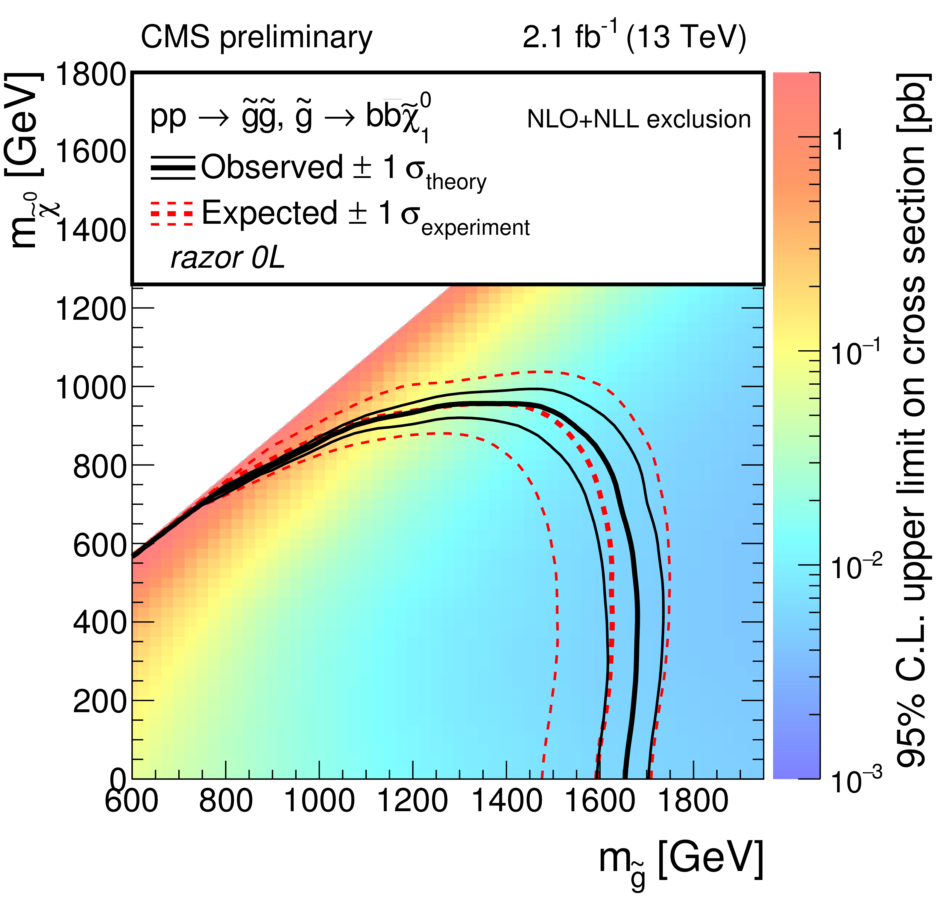
Figure 7:
Interpretation of the search results with razor variables in the context of the gluino pair-production simplified model, in which the gluino decays with a 100% branching fraction to a $ \mathrm{ b \bar{b} } $ pair and the LSP. The color coding indicates the observed 95% CL upper limit on the signal cross section. The dashed and solid lines represent the expected and observed exclusion contours at 95% CL, respectively. The solid contours around the observed limit and the dashed contours around the expected one represent the one standard deviation theoretical uncertainties in the cross section and the combination of the statistical and experimental systematic uncertainties, respectively. |
png ; pdf ; |
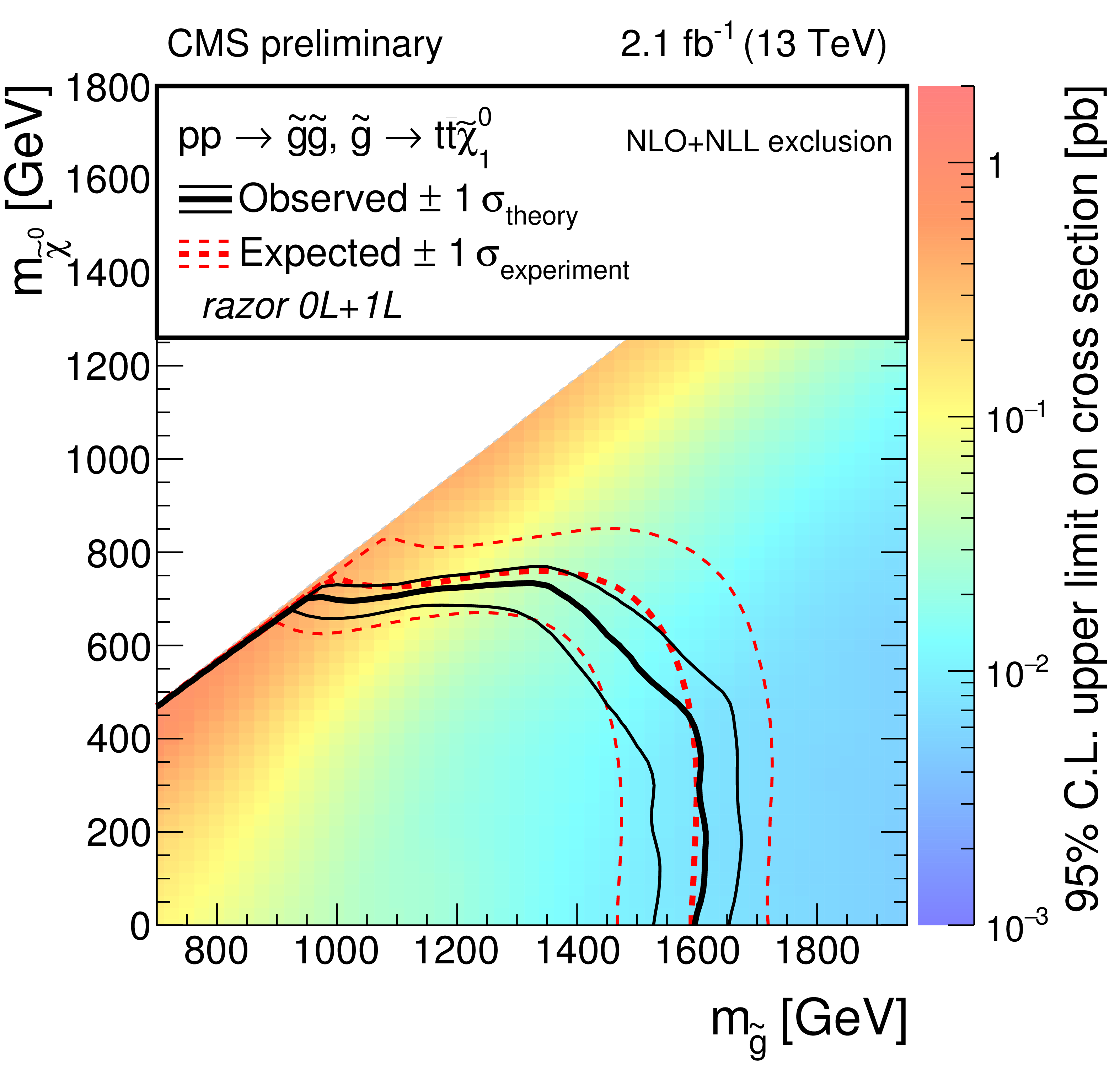
Figure 8:
Interpretation of the search results with razor variables in the context of the gluino pair-production simplified model, in which the gluino decays with a 100% branching fraction to a $ \mathrm{ t \bar{t} } $ pair and the LSP. The color coding indicates the observed 95% CL upper limit on the signal cross section. The dashed and solid lines represent the expected and observed exclusion contours at 95% CL, respectively. The solid contours around the observed limit and the dashed contours around the expected one represent the one standard deviation theoretical uncertainties in the cross section and the combination of the statistical and experimental systematic uncertainties, respectively. |
png ; pdf ; |
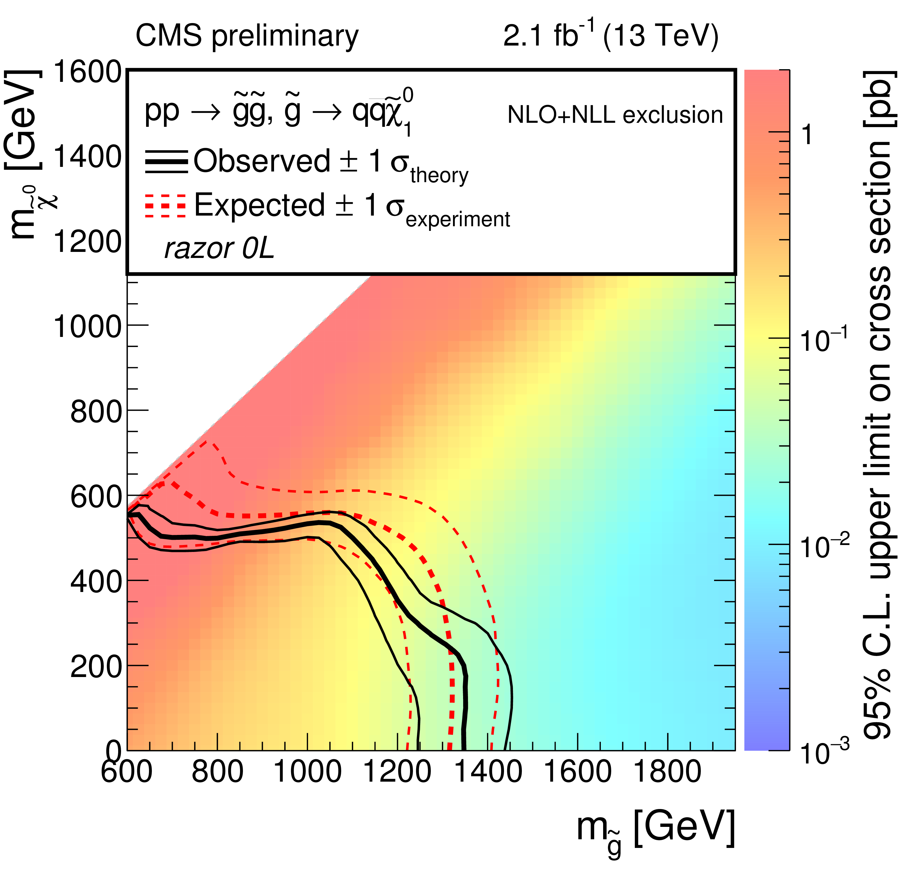
Figure 9:
Interpretation of the search results with razor variables in the context of the gluino pair-production simplified model, in which the gluino decays with a 100% branching fraction to a $ \mathrm{ q \bar{q} } $ pair and the LSP. The color coding indicates the observed 95% CL upper limit on the signal cross section. The dashed and solid lines represent the expected and observed exclusion contours at 95% CL, respectively. The solid contours around the observed limit and the dashed contours around the expected one represent the one standard deviation theoretical uncertainties in the cross section and the combination of the statistical and experimental systematic uncertainties, respectively. |
png ; pdf ; |
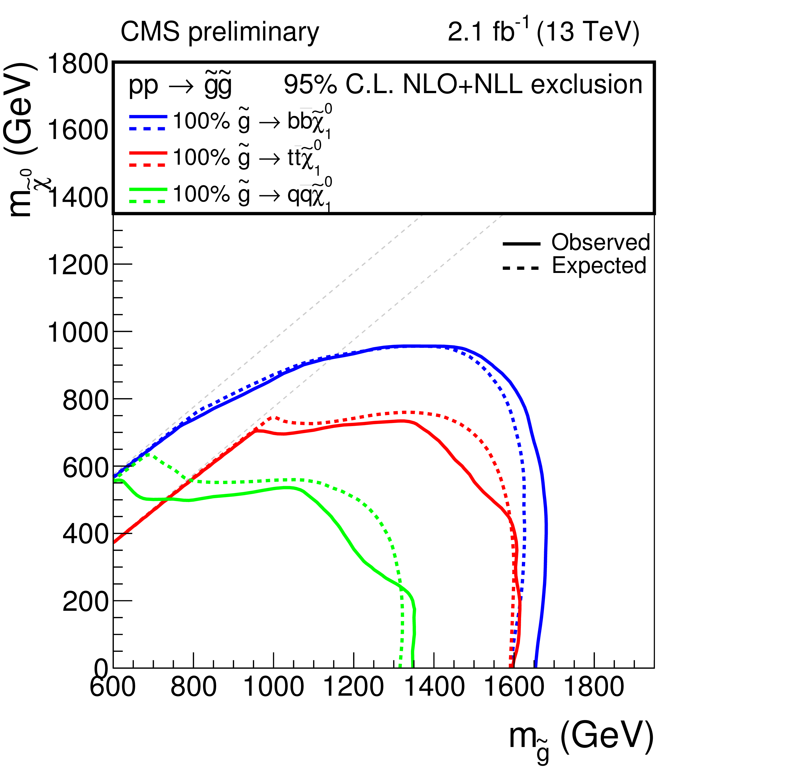
Figure 10:
Summary of the exclusion contours at 95% CL in the context of gluino pair-production simplified models signals, where gluinos decay with a 100% branching fraction to an LSP and a $ \mathrm{ t \bar{t} } $, $ \mathrm{ t \bar{t} } $, and $ \mathrm{ q \bar{q} } $ pair respectively. The dashed and solid lines represent the expected and observed exclusion contours at 95% CL, respectively. The two dashed diagonal lines indicate the boundaries of the respective mass scans ($m_{\tilde{g}} = m_{\tilde{\chi }^0} +$ 25 GeV for the simplified model with bottom quarks and first or second generation quarks in the final state and $m_{\tilde{g}} = m_{\tilde{\chi }^0} +$ 225 GeV for for the simplified model with top quarks in the final state). |
|
|
Compact Muon Solenoid LHC, CERN |
|

|

|

|

|

|