

Compact Muon Solenoid
LHC, CERN
| CMS-PAS-MLG-24-001 | ||
| Reweighting of simulated events using machine learning techniques in CMS | ||
| CMS Collaboration | ||
| 19 July 2024 | ||
| Abstract: Data analyses in particle physics rely on the accurate simulation of particle collisions and a detailed detector simulation to extract physical knowledge from the recorded data. Event generators together with a GEANT-based simulation of the detectors are used to produce large samples of simulated events for analysis by the LHC experiments. These simulations come at a high computational cost, where the detector simulation and reconstruction algorithms have the largest CPU demands. This note describes how machine learning (ML) techniques are used to reweight simulated samples to different model parameters or entirely different models. The ML method avoids the need for simulating the detector response multiple times by incorporating the relevant information in a single sample through event weights. Results are presented for reweightings to model variations and higher-order calculations in simulated top quark pair production at the LHC. This ML-based reweighting is an important element of the future computing model of the CMS Collaboration and will enable precision measurements with the CMS experiment at the High-Luminosity LHC. | ||
|
Links:
CDS record (PDF) ;
Physics Briefing ;
CADI line (restricted) ;
These preliminary results are superseded in this paper, Submitted to CSBS. The superseded preliminary plots can be found here. |
||
| Figures | |

png pdf |
Figure 1:
The normalised differential cross section of $ \mathrm{t} \overline{\mathrm{t}} $ production in pp collisions at 13 TeV as a function of the $ p_{\mathrm{T}} $ (left) and $ \eta $ (right) of the $ {\mathrm{t}\overline{\mathrm{t}}} $ system obtained with the POWHEG program. The standard setting of $ h_\text{{damp}} = 1.379 m_{\mathrm{t}} $ (black) is compared to down (green) and up (magenta) variations in $ h_\text{{damp}} $. The ratios of the predictions with the $ h_\text{{damp}} $ variations to the nominal one are shown in the lower panels. The error bars represent the statistical uncertainties in the MC samples. |

png pdf |
Figure 1-a:
The normalised differential cross section of $ \mathrm{t} \overline{\mathrm{t}} $ production in pp collisions at 13 TeV as a function of the $ p_{\mathrm{T}} $ (left) and $ \eta $ (right) of the $ {\mathrm{t}\overline{\mathrm{t}}} $ system obtained with the POWHEG program. The standard setting of $ h_\text{{damp}} = 1.379 m_{\mathrm{t}} $ (black) is compared to down (green) and up (magenta) variations in $ h_\text{{damp}} $. The ratios of the predictions with the $ h_\text{{damp}} $ variations to the nominal one are shown in the lower panels. The error bars represent the statistical uncertainties in the MC samples. |

png pdf |
Figure 1-b:
The normalised differential cross section of $ \mathrm{t} \overline{\mathrm{t}} $ production in pp collisions at 13 TeV as a function of the $ p_{\mathrm{T}} $ (left) and $ \eta $ (right) of the $ {\mathrm{t}\overline{\mathrm{t}}} $ system obtained with the POWHEG program. The standard setting of $ h_\text{{damp}} = 1.379 m_{\mathrm{t}} $ (black) is compared to down (green) and up (magenta) variations in $ h_\text{{damp}} $. The ratios of the predictions with the $ h_\text{{damp}} $ variations to the nominal one are shown in the lower panels. The error bars represent the statistical uncertainties in the MC samples. |

png pdf |
Figure 2:
The NN histories of the training for the $ h_\text{{damp}} $ parameter reweighting. Shown are the loss functions for the training data (blue) and the validation data (orange) for the down (left) and up (right) variations of $ h_\text{{damp}} $. |

png pdf |
Figure 2-a:
The NN histories of the training for the $ h_\text{{damp}} $ parameter reweighting. Shown are the loss functions for the training data (blue) and the validation data (orange) for the down (left) and up (right) variations of $ h_\text{{damp}} $. |

png pdf |
Figure 2-b:
The NN histories of the training for the $ h_\text{{damp}} $ parameter reweighting. Shown are the loss functions for the training data (blue) and the validation data (orange) for the down (left) and up (right) variations of $ h_\text{{damp}} $. |

png pdf |
Figure 3:
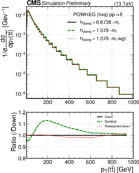
The normalised differential cross section as a function of the $ p_{\mathrm{T}} $ (upper) and $ \eta $ (lower) of the $ {\mathrm{t}\overline{\mathrm{t}}} $ system. The black line shows the predictions from the down (left) and up (right) variations in $ h_\text{{damp}} $, and the green line shows the prediction from the nominal sample. The red line shows the nominal sample reweighted to the down (left) and up (right) $ h_\text{{damp}} $ variations using the DCTR method. The ratios to the samples with the target values of $ h_\text{{damp}} $ are shown below the distributions. Vertical bars represent statistical uncertainties. |
png pdf |
Figure 3-a:
The normalised differential cross section as a function of the $ p_{\mathrm{T}} $ (upper) and $ \eta $ (lower) of the $ {\mathrm{t}\overline{\mathrm{t}}} $ system. The black line shows the predictions from the down (left) and up (right) variations in $ h_\text{{damp}} $, and the green line shows the prediction from the nominal sample. The red line shows the nominal sample reweighted to the down (left) and up (right) $ h_\text{{damp}} $ variations using the DCTR method. The ratios to the samples with the target values of $ h_\text{{damp}} $ are shown below the distributions. Vertical bars represent statistical uncertainties. |

png pdf |
Figure 3-b:
The normalised differential cross section as a function of the $ p_{\mathrm{T}} $ (upper) and $ \eta $ (lower) of the $ {\mathrm{t}\overline{\mathrm{t}}} $ system. The black line shows the predictions from the down (left) and up (right) variations in $ h_\text{{damp}} $, and the green line shows the prediction from the nominal sample. The red line shows the nominal sample reweighted to the down (left) and up (right) $ h_\text{{damp}} $ variations using the DCTR method. The ratios to the samples with the target values of $ h_\text{{damp}} $ are shown below the distributions. Vertical bars represent statistical uncertainties. |

png pdf |
Figure 3-c:
The normalised differential cross section as a function of the $ p_{\mathrm{T}} $ (upper) and $ \eta $ (lower) of the $ {\mathrm{t}\overline{\mathrm{t}}} $ system. The black line shows the predictions from the down (left) and up (right) variations in $ h_\text{{damp}} $, and the green line shows the prediction from the nominal sample. The red line shows the nominal sample reweighted to the down (left) and up (right) $ h_\text{{damp}} $ variations using the DCTR method. The ratios to the samples with the target values of $ h_\text{{damp}} $ are shown below the distributions. Vertical bars represent statistical uncertainties. |

png pdf |
Figure 3-d:
The normalised differential cross section as a function of the $ p_{\mathrm{T}} $ (upper) and $ \eta $ (lower) of the $ {\mathrm{t}\overline{\mathrm{t}}} $ system. The black line shows the predictions from the down (left) and up (right) variations in $ h_\text{{damp}} $, and the green line shows the prediction from the nominal sample. The red line shows the nominal sample reweighted to the down (left) and up (right) $ h_\text{{damp}} $ variations using the DCTR method. The ratios to the samples with the target values of $ h_\text{{damp}} $ are shown below the distributions. Vertical bars represent statistical uncertainties. |

png pdf |
Figure 4:
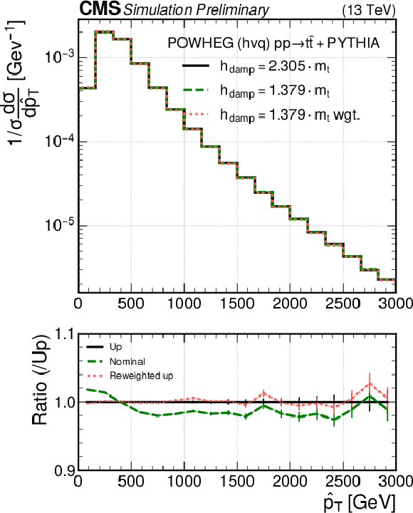
The normalised differential cross section as a function of $ N_{jet} $ (left) and $ \hat{p_{\mathrm{T}}} $ (right). The black line shows the predictions from the up variation in $ h_\text{{damp}} $ and the green line shows the prediction from the nominal sample. The red line shows the nominal sample reweighted to the $ h_\text{{damp}} $ variation using the DCTR method. The ratios to the target distributions are shown in the pads below. Vertical bars represent statistical uncertainties. |

png pdf |
Figure 4-a:
The normalised differential cross section as a function of $ N_{jet} $ (left) and $ \hat{p_{\mathrm{T}}} $ (right). The black line shows the predictions from the up variation in $ h_\text{{damp}} $ and the green line shows the prediction from the nominal sample. The red line shows the nominal sample reweighted to the $ h_\text{{damp}} $ variation using the DCTR method. The ratios to the target distributions are shown in the pads below. Vertical bars represent statistical uncertainties. |
png pdf |
Figure 4-b:
The normalised differential cross section as a function of $ N_{jet} $ (left) and $ \hat{p_{\mathrm{T}}} $ (right). The black line shows the predictions from the up variation in $ h_\text{{damp}} $ and the green line shows the prediction from the nominal sample. The red line shows the nominal sample reweighted to the $ h_\text{{damp}} $ variation using the DCTR method. The ratios to the target distributions are shown in the pads below. Vertical bars represent statistical uncertainties. |

png pdf |
Figure 5:
Ratios between the $ h_\text{{damp}} $ target distributions in $ p_{\mathrm{T}}({\mathrm{t}\overline{\mathrm{t}}} ) $ (left) and $ \eta({\mathrm{t}\overline{\mathrm{t}}} ) $ (right), and 50 different reweightings (grey lines). The ratio to the target before the reweighting is shown as a green dashed line and the mean of the different reweightings as a red dashed line. The red band represents the statistical uncertainty of the method obtained from the standard deviation of the 50 reweightings. |

png pdf |
Figure 5-a:
Ratios between the $ h_\text{{damp}} $ target distributions in $ p_{\mathrm{T}}({\mathrm{t}\overline{\mathrm{t}}} ) $ (left) and $ \eta({\mathrm{t}\overline{\mathrm{t}}} ) $ (right), and 50 different reweightings (grey lines). The ratio to the target before the reweighting is shown as a green dashed line and the mean of the different reweightings as a red dashed line. The red band represents the statistical uncertainty of the method obtained from the standard deviation of the 50 reweightings. |

png pdf |
Figure 5-b:
Ratios between the $ h_\text{{damp}} $ target distributions in $ p_{\mathrm{T}}({\mathrm{t}\overline{\mathrm{t}}} ) $ (left) and $ \eta({\mathrm{t}\overline{\mathrm{t}}} ) $ (right), and 50 different reweightings (grey lines). The ratio to the target before the reweighting is shown as a green dashed line and the mean of the different reweightings as a red dashed line. The red band represents the statistical uncertainty of the method obtained from the standard deviation of the 50 reweightings. |
png pdf |
Figure 6:
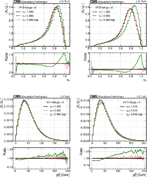
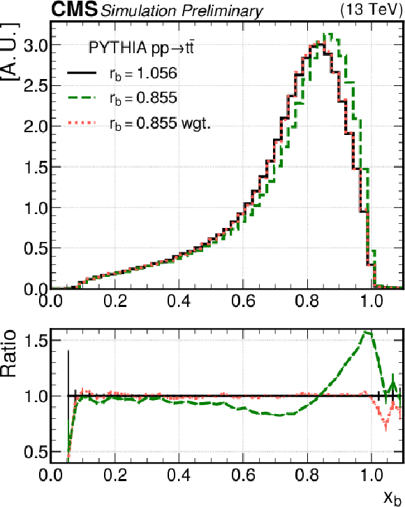
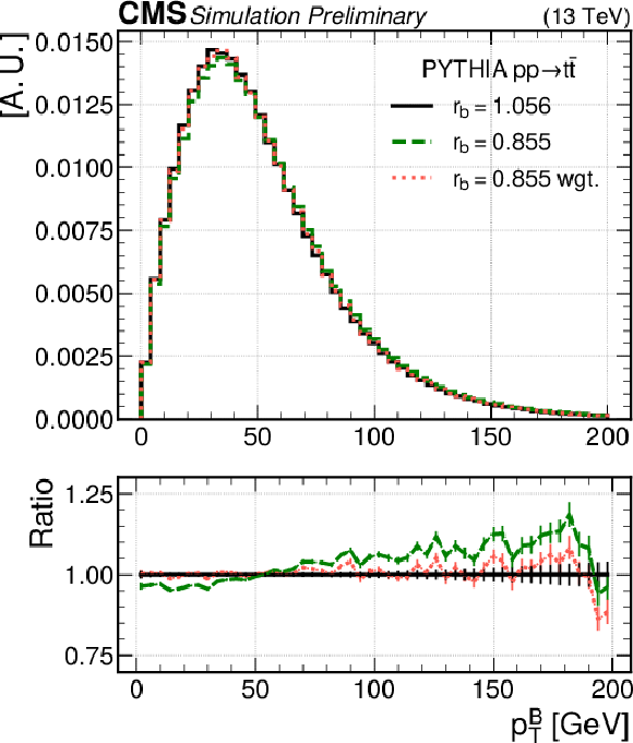
Distributions in $ x_{\mathrm{b}} $ (upper) and $ p_{\mathrm{T},{\mathrm{B}}} $ (lower) from $ \mathrm{t} \overline{\mathrm{t}} $ simulations with PYTHIA 8 with value $ r_{\mathrm{b}}= $ 0.855 (dashed green line) and a second value of $ r_{\mathrm{b}} $ (solid black line). The nominal sample reweighted to $ r_{\mathrm{b}}= $ 1.056 (left) and $ r_{\mathrm{b}}= $ 1.252 (right) are is shown as red dotted lines. Below each distribution, the ratios to the target distribution are shown. The vertical bars represent the statistical uncertainties. |
png pdf |
Figure 6-a:
Distributions in $ x_{\mathrm{b}} $ (upper) and $ p_{\mathrm{T},{\mathrm{B}}} $ (lower) from $ \mathrm{t} \overline{\mathrm{t}} $ simulations with PYTHIA 8 with value $ r_{\mathrm{b}}= $ 0.855 (dashed green line) and a second value of $ r_{\mathrm{b}} $ (solid black line). The nominal sample reweighted to $ r_{\mathrm{b}}= $ 1.056 (left) and $ r_{\mathrm{b}}= $ 1.252 (right) are is shown as red dotted lines. Below each distribution, the ratios to the target distribution are shown. The vertical bars represent the statistical uncertainties. |

png pdf |
Figure 6-b:
Distributions in $ x_{\mathrm{b}} $ (upper) and $ p_{\mathrm{T},{\mathrm{B}}} $ (lower) from $ \mathrm{t} \overline{\mathrm{t}} $ simulations with PYTHIA 8 with value $ r_{\mathrm{b}}= $ 0.855 (dashed green line) and a second value of $ r_{\mathrm{b}} $ (solid black line). The nominal sample reweighted to $ r_{\mathrm{b}}= $ 1.056 (left) and $ r_{\mathrm{b}}= $ 1.252 (right) are is shown as red dotted lines. Below each distribution, the ratios to the target distribution are shown. The vertical bars represent the statistical uncertainties. |
png pdf |
Figure 6-c:
Distributions in $ x_{\mathrm{b}} $ (upper) and $ p_{\mathrm{T},{\mathrm{B}}} $ (lower) from $ \mathrm{t} \overline{\mathrm{t}} $ simulations with PYTHIA 8 with value $ r_{\mathrm{b}}= $ 0.855 (dashed green line) and a second value of $ r_{\mathrm{b}} $ (solid black line). The nominal sample reweighted to $ r_{\mathrm{b}}= $ 1.056 (left) and $ r_{\mathrm{b}}= $ 1.252 (right) are is shown as red dotted lines. Below each distribution, the ratios to the target distribution are shown. The vertical bars represent the statistical uncertainties. |

png pdf |
Figure 6-d:
Distributions in $ x_{\mathrm{b}} $ (upper) and $ p_{\mathrm{T},{\mathrm{B}}} $ (lower) from $ \mathrm{t} \overline{\mathrm{t}} $ simulations with PYTHIA 8 with value $ r_{\mathrm{b}}= $ 0.855 (dashed green line) and a second value of $ r_{\mathrm{b}} $ (solid black line). The nominal sample reweighted to $ r_{\mathrm{b}}= $ 1.056 (left) and $ r_{\mathrm{b}}= $ 1.252 (right) are is shown as red dotted lines. Below each distribution, the ratios to the target distribution are shown. The vertical bars represent the statistical uncertainties. |
png pdf |
Figure 7:
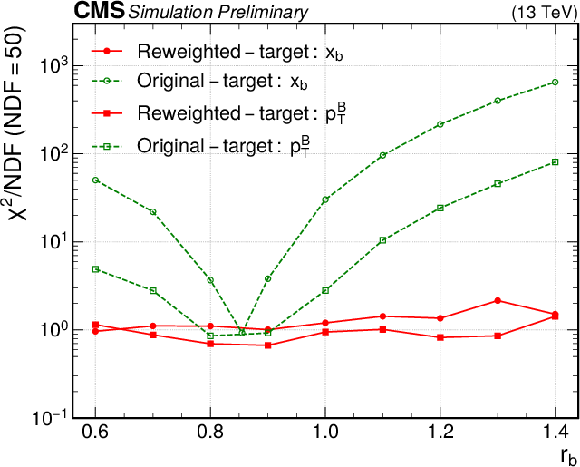
Values of $ \chi^{2}/\text{NDF} $ obtained for distributions in $ x_{\mathrm{b}} $ (circles) and $ p_{\mathrm{T}}^{{\mathrm{B}}} $ (squares), where target distributions for events with different $ r_{\mathrm{b}} $ values are compared to a distribution with the nominal value of $ r_{\mathrm{b}}= $ 0.855 before the reweighting (green) and after the reweighting to the target value of $ r_{\mathrm{b}} $ (red). The lines connecting the markers are shown for illustration purposes only. |

png pdf |
Figure 8:
Distributions in top quark $ p_{\mathrm{T}} $ (left) and $ \eta $ (right) obtained from simulations at NNLO accuracy (black solid lines), NLO accuracy (green dashed lines), and NLO reweighted to NNLO with the DCTR method (red dotted lines). The ratio to the NNLO predictions is shown in the lower panels, where the vertical bars correspond to the statistical uncertainties. |

png pdf |
Figure 8-a:
Distributions in top quark $ p_{\mathrm{T}} $ (left) and $ \eta $ (right) obtained from simulations at NNLO accuracy (black solid lines), NLO accuracy (green dashed lines), and NLO reweighted to NNLO with the DCTR method (red dotted lines). The ratio to the NNLO predictions is shown in the lower panels, where the vertical bars correspond to the statistical uncertainties. |

png pdf |
Figure 8-b:
Distributions in top quark $ p_{\mathrm{T}} $ (left) and $ \eta $ (right) obtained from simulations at NNLO accuracy (black solid lines), NLO accuracy (green dashed lines), and NLO reweighted to NNLO with the DCTR method (red dotted lines). The ratio to the NNLO predictions is shown in the lower panels, where the vertical bars correspond to the statistical uncertainties. |

png pdf |
Figure 9:
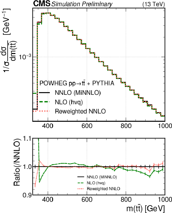
Distributions in $ p_{\mathrm{T}} $ (upper left), $ \eta $ (upper right), $ \Delta\phi $ (lower left), and mass (lower right) of the $ \mathrm{t} \overline{\mathrm{t}} $ system obtained from simulations at NNLO accuracy (black solid lines), NLO accuracy (green dashed lines), and NLO reweighted to NNLO with the DCTR method (red dotted lines). The ratio to the NNLO predictions is shown in the lower panels, where the vertical bars correspond to the statistical uncertainties. |

png pdf |
Figure 9-a:
Distributions in $ p_{\mathrm{T}} $ (upper left), $ \eta $ (upper right), $ \Delta\phi $ (lower left), and mass (lower right) of the $ \mathrm{t} \overline{\mathrm{t}} $ system obtained from simulations at NNLO accuracy (black solid lines), NLO accuracy (green dashed lines), and NLO reweighted to NNLO with the DCTR method (red dotted lines). The ratio to the NNLO predictions is shown in the lower panels, where the vertical bars correspond to the statistical uncertainties. |

png pdf |
Figure 9-b:
Distributions in $ p_{\mathrm{T}} $ (upper left), $ \eta $ (upper right), $ \Delta\phi $ (lower left), and mass (lower right) of the $ \mathrm{t} \overline{\mathrm{t}} $ system obtained from simulations at NNLO accuracy (black solid lines), NLO accuracy (green dashed lines), and NLO reweighted to NNLO with the DCTR method (red dotted lines). The ratio to the NNLO predictions is shown in the lower panels, where the vertical bars correspond to the statistical uncertainties. |

png pdf |
Figure 9-c:
Distributions in $ p_{\mathrm{T}} $ (upper left), $ \eta $ (upper right), $ \Delta\phi $ (lower left), and mass (lower right) of the $ \mathrm{t} \overline{\mathrm{t}} $ system obtained from simulations at NNLO accuracy (black solid lines), NLO accuracy (green dashed lines), and NLO reweighted to NNLO with the DCTR method (red dotted lines). The ratio to the NNLO predictions is shown in the lower panels, where the vertical bars correspond to the statistical uncertainties. |
png pdf |
Figure 9-d:
Distributions in $ p_{\mathrm{T}} $ (upper left), $ \eta $ (upper right), $ \Delta\phi $ (lower left), and mass (lower right) of the $ \mathrm{t} \overline{\mathrm{t}} $ system obtained from simulations at NNLO accuracy (black solid lines), NLO accuracy (green dashed lines), and NLO reweighted to NNLO with the DCTR method (red dotted lines). The ratio to the NNLO predictions is shown in the lower panels, where the vertical bars correspond to the statistical uncertainties. |

png pdf |
Figure 10:
Distributions in $ p_{\mathrm{T}} $ of the $ \mathrm{t} \overline{\mathrm{t}} $ system (left) and $ p_{\mathrm{T}} $ of the t (right) obtained from simulations at NNLO accuracy (black solid lines), NLO accuracy (green dashed lines), NLO reweighted to NNLO with the DCTR method (red dotted lines), and NLO reweighted using a two-dimensional reweighting in $ p_{\mathrm{T}} $ of the $ \mathrm{t} \overline{\mathrm{t}} $ system and of the t (blue dash-dotted line). The ratio to the NNLO predictions is shown in the lower panels, where the vertical bars correspond to the statistical uncertainties. |

png pdf |
Figure 10-a:
Distributions in $ p_{\mathrm{T}} $ of the $ \mathrm{t} \overline{\mathrm{t}} $ system (left) and $ p_{\mathrm{T}} $ of the t (right) obtained from simulations at NNLO accuracy (black solid lines), NLO accuracy (green dashed lines), NLO reweighted to NNLO with the DCTR method (red dotted lines), and NLO reweighted using a two-dimensional reweighting in $ p_{\mathrm{T}} $ of the $ \mathrm{t} \overline{\mathrm{t}} $ system and of the t (blue dash-dotted line). The ratio to the NNLO predictions is shown in the lower panels, where the vertical bars correspond to the statistical uncertainties. |

png pdf |
Figure 10-b:
Distributions in $ p_{\mathrm{T}} $ of the $ \mathrm{t} \overline{\mathrm{t}} $ system (left) and $ p_{\mathrm{T}} $ of the t (right) obtained from simulations at NNLO accuracy (black solid lines), NLO accuracy (green dashed lines), NLO reweighted to NNLO with the DCTR method (red dotted lines), and NLO reweighted using a two-dimensional reweighting in $ p_{\mathrm{T}} $ of the $ \mathrm{t} \overline{\mathrm{t}} $ system and of the t (blue dash-dotted line). The ratio to the NNLO predictions is shown in the lower panels, where the vertical bars correspond to the statistical uncertainties. |
| Summary |
| Particle physics relies on the simulation of events using Monte Carlo (MC) event generators for data-to-theory comparisons. Data analyses require the production of several samples simulating the same physical process to estimate systematic uncertainties or the impact of higher-order calculations. To have statistically significant value, these samples have to be very large with millions of events generated and simulated at a high computational cost. Nevertheless, the statistical precision from the finite size of these samples can become a limiting factor in precision analyses. The production of sufficiently large MC samples, such that the statistical precision of these samples is better than the statistical precision of the data, will become increasingly prohibitive at the High-Luminosity LHC (HL-LHC) with the expected computing resources. Current estimates assume that 160 billion fully simulated and reconstructed MC events have to be produced per year after the start of the HL-LHC. This number may become larger by up to 30% because of negative events in next-to-leading order (NLO) and next-to-NLO (NNLO) simulations, which reduce the statistical precision of the MC samples. In this note, the deep neural network using classification for tuning and reweighting (DCTR) method has been introduced to reweight MC samples used in CMS analyses. The weights calculated with the DCTR model enable the modification of one central sample to mimic other samples obtained with different parameters or different simulation programs. This methodology avoids the need for simulating the detector response for multiple samples by incorporating the relevant variations in a single sample. While dedicated samples have to be generated for the training and validation of the model, these do not need to have the full detector simulation and reconstruction, saving up to 75% of the typical CPU resources needed for the production of MC samples in CMS. In addition, after the training of the DCTR model, the training samples can be deleted saving storage space for multiple billions of events. This method will become an integral part of the computing model of the CMS Collaboration for the HL-LHC. The DCTR method has been shown to work reliably for two important sources of modelling uncertainties in the simulation of top quark pair ($ \mathrm{t} \overline{\mathrm{t}} $) production. The systematic uncertainty connected to the matching of radiation from matrix elements and the parton shower previously had to be estimated with dedicated samples. The reweighting of variations in the b quark fragmentation shows that a continuous reweighting in a model parameter is possible, paving the way for the determination of model parameters directly from collision data. Additionally, the method has been extended to reweight an NLO simulation to an NNLO one for $ \mathrm{t} \overline{\mathrm{t}} $ production, which will allow for a fast evaluation of the impact of higher-order corrections on data analyses. The DCTR reweighting can be seamlessly integrated into CMS analyses, providing an elegant solution to address the computational challenges posed by the production of large MC samples, particularly for the HL-LHC. |
| References | ||||
| 1 | ATLAS Collaboration | ATLAS software and computing HL-LHC roadmap | Technical Report CERN-LHCC-2022-005, LHCC-G-182, 2022 | |
| 2 | CMS Offline Software and Computing Group | CMS Phase-2 computing model: Update document | CMS Note CMS-NOTE-2022-008, 2022 | |
| 3 | The HEP Software Foundation | A roadmap for HEP software and computing R&D for the 2020s | Comput. Softw. Big Sci. 3 (2019) 7 | 1712.06982 |
| 4 | G. Apollinari et al. | High-Luminosity Large Hadron Collider (HL-LHC): Technical design report | CERN Yellow Reports: Monographs, 2017 link |
|
| 5 | CMS Collaboration | Measurement of the $ \mathrm{t}\overline{\mathrm{t}} $ production cross section, the top quark mass, and the strong coupling constant using dilepton events in pp collisions at $ \sqrt{s} = $ 13 TeV | EPJC 79 (2019) 368 | CMS-TOP-17-001 1812.10505 |
| 6 | A. Rogozhnikov | Reweighting with boosted decision trees | J. Phys. Conf. Ser. 762 (2016) 012036 | 1608.05806 |
| 7 | K. Cranmer, J. Pavez, and G. Louppe | Approximating likelihood ratios with calibrated discriminative classifiers | 1506.02169 | |
| 8 | A. Andreassen and B. Nachman | Neural networks for full phase-space reweighting and parameter tuning | PRD 101 (2020) 091901 | 1907.08209 |
| 9 | B. Nachman and J. Thaler | Neural conditional reweighting | PRD 105 (2022) 076015 | 2107.08979 |
| 10 | B. Amos, L. Xu, and J. Z. Kolter | Input convex neural networks | in Proceedings of the 34th International Conference on Machine Learning, D. Precup and Y. W. Teh, eds., volume 70 of Proceedings of Machine Learning Research, PMLR, 2017 | 1609.07152 |
| 11 | C. Pollard and P. Windischhofer | Transport away your problems: Calibrating stochastic simulations with optimal transport | NIM A 1027 (2022) 166119 | 2107.08648 |
| 12 | E. G. Tabak and C. V. Turner | A family of nonparametric density estimation algorithms | Comm. Pure and Appl. Math. 66 (2013) 145 | |
| 13 | E. G. Tabak and E. Vanden-Eijnden | Density estimation by dual ascent of the log-likelihood | Comm. Math. Sci. 8 (2010) 217 | |
| 14 | T. Golling, S. Klein, R. Mastandrea, and B. Nachman | Flow-enhanced transportation for anomaly detection | PRD 107 (2023) 096025 | 2212.11285 |
| 15 | J. A. Raine, S. Klein, D. Sengupta, and T. Golling | CURTAINs for your sliding window: Constructing unobserved regions by transforming adjacent intervals | Front. Big Data 6 (2023) 899345 | 2203.09470 |
| 16 | A. Hallin et al. | Classifying anomalies through outer density estimation | PRD 106 (2022) 055006 | 2109.00546 |
| 17 | M. Algren et al. | Flow away your differences: Conditional normalizing flows as an improvement to reweighting | 2304.14963 | |
| 18 | S. Diefenbacher et al. | DCTRGAN: Improving the precision of generative models with reweighting | JINST 15 (2020) P11004 | 2009.03796 |
| 19 | S. Alioli, P. Nason, C. Oleari, and E. Re | A general framework for implementing NLO calculations in shower Monte Carlo programs: The POWHEG BOX | JHEP 06 (2010) 043 | 1002.2581 |
| 20 | S. Frixione, P. Nason, and G. Ridolfi | A positive-weight next-to-leading-order Monte Carlo for heavy flavour hadroproduction | JHEP 09 (2007) 126 | 0707.3088 |
| 21 | S. Frixione, P. Nason, and C. Oleari | Matching NLO QCD computations with parton shower simulations: The POWHEG method | JHEP 11 (2007) 070 | 0709.2092 |
| 22 | T. Sjöstrand et al. | An introduction to PYTHIA 8.2 | Comput. Phys. Commun. 191 (2015) 159 | 1410.3012 |
| 23 | P. T. Komiske, E. M. Metodiev, and J. Thaler | Energy flow networks: Deep sets for particle jets | JHEP 01 (2019) 121 | 1810.05165 |
| 24 | P. Baldi et al. | Parameterized neural networks for high-energy physics | EPJC 76 (2016) 235 | 1601.07913 |
| 25 | M. Zaheer et al. | Deep sets | 1703.06114 | |
| 26 | A. F. Agarap | Deep learning using rectified linear units (ReLU) | 1803.08375 | |
| 27 | F. Chollet et al. | Keras | https://keras.io | |
| 28 | R. L. T. Hahnloser | On the piecewise analysis of networks of linear threshold neurons | Neural Networks 11 (1998) 691 | |
| 29 | D. P. Kingma and J. Ba | Adam: A method for stochastic optimization | in International Conference on Learning Representations (ICLR) San Diega, CA, USA, 2014 | 1412.6980 |
| 30 | S. Alioli, P. Nason, C. Oleari, and E. Re | NLO Higgs boson production via gluon fusion matched with shower in POWHEG | JHEP 04 (2009) 002 | 0812.0578 |
| 31 | CMS Collaboration | Extraction and validation of a new set of CMS PYTHIA8 tunes from underlying-event measurements | EPJC 80 (2020) 4 | CMS-GEN-17-001 1903.12179 |
| 32 | M. Cacciari, G. P. Salam, and G. Soyez | The anti-$ k_{\mathrm{T}} $ jet clustering algorithm | JHEP 04 (2008) 063 | 0802.1189 |
| 33 | C. Bierlich et al. | A comprehensive guide to the physics and usage of PYTHIA 8.3 | SciPost Phys. Codeb. 2022 (2022) 8 | 2203.11601 |
| 34 | M. G. Bowler | $ \mathrm{e}^+ \mathrm{e}^- $ production of heavy quarks in the string model | Z. Phys. C 11 (1981) 169 | |
| 35 | P. Skands, S. Carrazza, and J. Rojo | Tuning PYTHIA 8.1: The Monash 2013 tune | EPJC 74 (2014) 3024 | 1404.5630 |
| 36 | G. Corcella and A. D. Mitov | Bottom quark fragmentation in top quark decay | NPB 623 (2002) 247 | hep-ph/0110319 |
| 37 | M. Cacciari, G. Corcella, and A. D. Mitov | Soft gluon resummation for bottom fragmentation in top quark decay | JHEP 12 (2002) 015 | hep-ph/0209204 |
| 38 | P. B ä rnreuther, M. Czakon, and A. Mitov | Percent level precision physics at the Tevatron: First genuine NNLO QCD corrections to $ \mathrm{q} \overline{\mathrm{q}} \to {\mathrm{t}\overline{\mathrm{t}}} + \mathrm{X} $ | PRL 109 (2012) 132001 | 1204.5201 |
| 39 | M. Czakon and A. Mitov | NNLO corrections to top-pair production at hadron colliders: The all-fermionic scattering channels | JHEP 12 (2012) 054 | 1207.0236 |
| 40 | M. Czakon and A. Mitov | NNLO corrections to top pair production at hadron colliders: The quark-gluon reaction | JHEP 01 (2013) 080 | 1210.6832 |
| 41 | M. Czakon, P. Fiedler, and A. Mitov | Total top-quark pair-production cross section at hadron colliders through $ O(\alpha^4_S) $ | PRL 110 (2013) 252004 | 1303.6254 |
| 42 | M. Czakon, D. Heymes, and A. Mitov | High-precision differential predictions for top-quark pairs at the LHC | PRL 116 (2016) 082003 | 1511.00549 |
| 43 | M. Czakon, P. Fiedler, D. Heymes, and A. Mitov | NNLO QCD predictions for fully-differential top-quark pair production at the Tevatron | JHEP 05 (2016) 034 | 1601.05375 |
| 44 | S. Catani et al. | Top-quark pair hadroproduction at next-to-next-to-leading order in QCD | PRD 99 (2019) 051501 | 1901.04005 |
| 45 | S. Catani et al. | Top-quark pair production at the LHC: Fully differential QCD predictions at NNLO | JHEP 07 (2019) 100 | 1906.06535 |
| 46 | S. Catani et al. | Top-quark pair hadroproduction at NNLO: Differential predictions with the $ \overline{\text{MS}} $ mass | JHEP 08 (2020) 027 | 2005.00557 |
| 47 | CMS Collaboration | Measurement of differential cross sections for top quark pair production using the lepton+jets final state in proton-proton collisions at 13 TeV | PRD 95 (2017) 092001 | CMS-TOP-16-008 1610.04191 |
| 48 | CMS Collaboration | Measurement of double-differential cross sections for top quark pair production in pp collisions at $ \sqrt{s} = $ 8 TeV and impact on parton distribution functions | EPJC 77 (2017) 459 | CMS-TOP-14-013 1703.01630 |
| 49 | CMS Collaboration | Measurement of normalized differential $ \mathrm{t} \overline{\mathrm{t}} $ cross sections in the dilepton channel from pp collisions at $ \sqrt{s} = $ 13 TeV | JHEP 04 (2018) 060 | CMS-TOP-16-007 1708.07638 |
| 50 | CMS Collaboration | Measurements of differential cross sections of top quark pair production as a function of kinematic event variables in proton-proton collisions at $ \sqrt{s}= $ 13 TeV | JHEP 06 (2018) 002 | CMS-TOP-16-014 1803.03991 |
| 51 | CMS Collaboration | Measurements of $ \mathrm{t} \overline{\mathrm{t}} $ differential cross sections in proton-proton collisions at $ \sqrt{s}= $ 13 TeV using events containing two leptons | JHEP 02 (2019) 149 | CMS-TOP-17-014 1811.06625 |
| 52 | CMS Collaboration | Measurement of the top quark mass in the all-jets final state at $ \sqrt{s} = $ 13 TeV and combination with the lepton+jets channel | EPJC 79 (2019) 313 | CMS-TOP-17-008 1812.10534 |
| 53 | CMS Collaboration | Measurement of $ \mathrm{t} \overline{\mathrm{t}} $ normalised multi-differential cross sections in pp collisions at $ \sqrt{s}= $ 13 TeV, and simultaneous determination of the strong coupling strength, top quark pole mass, and parton distribution functions | EPJC 80 (2020) 658 | CMS-TOP-18-004 1904.05237 |
| 54 | CMS Collaboration | Measurement of differential $ \mathrm{t} \overline{\mathrm{t}} $ production cross sections in the full kinematic range using lepton+jets events from proton-proton collisions at $ \sqrt{s} = $ 13 TeV | PRD 104 (2021) 092013 | CMS-TOP-20-001 2108.02803 |
| 55 | ATLAS Collaboration | Measurements of top-quark pair differential cross-sections in the lepton+jets channel in pp collisions at $ \sqrt{s}= $ 8 TeV using the ATLAS detector | EPJC 76 (2016) 538 | 1511.04716 |
| 56 | ATLAS Collaboration | Measurement of top quark pair differential cross-sections in the dilepton channel in pp collisions at $ \sqrt{s} = $ 7 and 8 TeV with ATLAS | PRD 94 (2016) 092003 | 1607.07281 |
| 57 | ATLAS Collaboration | Measurements of top-quark pair differential cross-sections in the $ {\mathrm{e}\mu} $ channel in pp collisions at $ \sqrt{s} = $ 13 TeV using the ATLAS detector | EPJC 77 (2017) 292 | 1612.05220 |
| 58 | ATLAS Collaboration | Measurements of top-quark pair differential cross-sections in the lepton+jets channel in pp collisions at $ \sqrt{s}= $ 13 TeV using the ATLAS detector | JHEP 11 (2017) 191 | 1708.00727 |
| 59 | ATLAS Collaboration | Measurement of lepton differential distributions and the top quark mass in $ \mathrm{t} \overline{\mathrm{t}} $ production in pp collisions at $ \sqrt{s}= $8 TeV with the ATLAS detector | EPJC 77 (2017) 804 | 1709.09407 |
| 60 | ATLAS Collaboration | Measurements of top-quark pair differential and double-differential cross-sections in the $ \ell $+jets channel with pp collisions at $ \sqrt{s}= $ 13 TeV using the ATLAS detector | EPJC 79 (2019) 1028 | 1908.07305 |
| 61 | ATLAS Collaboration | Measurement of the $ \mathrm{t} \overline{\mathrm{t}} $ production cross-section and lepton differential distributions in $ {\mathrm{e}\mu} $ dilepton events from pp collisions at $ \sqrt{s}= $ 13 TeV with the ATLAS detector | EPJC 80 (2020) 528 | 1910.08819 |
| 62 | M. Beneke, P. Falgari, S. Klein, and C. Schwinn | Hadronic top-quark pair production with NNLL threshold resummation | NPB 855 (2012) 695 | 1109.1536 |
| 63 | M. Beneke et al. | Inclusive top-pair production phenomenology with TOPIXS | JHEP 07 (2012) 194 | 1206.2454 |
| 64 | H. X. Zhu et al. | Transverse-momentum resummation for top-quark pairs at hadron colliders | PRL 110 (2013) 082001 | 1208.5774 |
| 65 | H. T. Li et al. | Top quark pair production at small transverse momentum in hadronic collisions | PRD 88 (2013) 074004 | 1307.2464 |
| 66 | S. Catani, M. Grazzini, and A. Torre | Transverse-momentum resummation for heavy-quark hadroproduction | NPB 890 (2014) 518 | 1408.4564 |
| 67 | S. Catani, M. Grazzini, and H. Sargsyan | Transverse-momentum resummation for top-quark pair production at the LHC | JHEP 11 (2018) 061 | 1806.01601 |
| 68 | W.-L. Ju et al. | Top quark pair production near threshold: Single/double distributions and mass determination | JHEP 06 (2020) 158 | 2004.03088 |
| 69 | S. Alioli, A. Broggio, and M. A. Lim | Zero-jettiness resummation for top-quark pair production at the LHC | JHEP 01 (2022) 066 | 2111.03632 |
| 70 | K. Hamilton, P. Nason, C. Oleari, and G. Zanderighi | Merging H/W/Z+0 and 1 jet at NLO with no merging scale: A path to parton shower+NNLO matching | JHEP 05 (2013) 082 | 1212.4504 |
| 71 | S. Alioli et al. | Matching fully differential NNLO calculations and parton showers | JHEP 06 (2014) 089 | 1311.0286 |
| 72 | S. Höche, Y. Li, and S. Prestel | Drell--Yan lepton pair production at NNLO QCD with parton showers | PRD 91 (2015) 074015 | 1405.3607 |
| 73 | P. F. Monni et al. | MiNNLO$ _{\text{PS}} $: A new method to match NNLO QCD to parton showers | JHEP 05 (2020) 143 | 1908.06987 |
| 74 | P. F. Monni, E. Re, and M. Wiesemann | MiNNLO$ _{\text {PS}} $: Optimizing 2 $ \to $ 1 hadronic processes | EPJC 80 (2020) 1075 | 2006.04133 |
| 75 | J. Mazzitelli et al. | Next-to-next-to-leading order event generation for top-quark pair production | PRL 127 (2021) 062001 | 2012.14267 |
| 76 | J. Mazzitelli et al. | Top-pair production at the LHC with MINNLO$ _{\text{PS}} $ | JHEP 04 (2022) 079 | 2112.12135 |
| 77 | CMS Collaboration | Search for a heavy resonance decaying to a top quark and a W boson at $ \sqrt{s}= $ 13 TeV in the fully hadronic final state | JHEP 12 (2021) 106 | 2104.12853 |
| 78 | CMS Collaboration | Search for a heavy resonance decaying into a top quark and a W boson in the lepton+jets final state at $ \sqrt{s}= $ 13 TeV | JHEP 04 (2022) 048 | 2111.10216 |
| 79 | ATLAS Collaboration | Measurements of differential cross-sections in top-quark pair events with a high transverse momentum top quark and limits on beyond the standard model contributions to top-quark pair production with the ATLAS detector at $ \sqrt{s} = $ 13 TeV | JHEP 06 (2022) 063 | 2202.12134 |
| 80 | B. Nachman and J. Thaler | Neural resampler for Monte Carlo reweighting with preserved uncertainties | PRD 102 (2020) 076004 | 2007.11586 |
| 81 | Open neural network exchange | (ONNX) | https://onnx.ai | |
| 82 | M. Abadi et al. | TensorFlow: Large-scale machine learning on heterogeneous systems | Software available from tensorflow.org link |
|
| 83 | A. Paszke et al. | PyTorch: An imperative style, high-performance deep learning library | 1912.01703 | |
| 84 | T. Chen and C. Guestrin | XGBoost: A scalable tree boosting system | 1603.02754 | |

|
Compact Muon Solenoid LHC, CERN |

|

|

|

|

|

|