

Compact Muon Solenoid
LHC, CERN
| ATLAS-CONF-2015-044; CMS-PAS-HIG-15-002 | ||
| Measurements of the Higgs boson production and decay rates and constraints on its couplings from a combined ATLAS and CMS analysis of the LHC $pp$ collision data at $\sqrt{s} =$ 7 and 8 TeV | ||
| ATLAS and CMS Collaborations | ||
| September 2015 | ||
| Abstract: Combined ATLAS and CMS measurements of the Higgs boson production and decay rates, as well as constraints on its couplings to vector bosons and fermions, are presented. The combination is based on the analysis of five production processes and of the $H \to ZZ$, $WW$, $\gamma\gamma$, $\tau\tau$, $bb$ and $\mu\mu$ decay modes. All results are reported assuming a value of 125.09 GeV for the Higgs boson mass, the result of the combined Higgs boson mass measurement by ATLAS and CMS. The analysis uses the LHC proton-proton collision datasets recorded by the ATLAS and CMS detectors in 2011 and 2012, corresponding to integrated luminosities per experiment of approximately 5 fb$^{-1}$ at $\sqrt{s}=$ 7 TeV and 20 fb$^{-1}$ at $\sqrt{s} =$ 8 TeV. The Higgs boson production and decay rates of the two experiments are combined within the context of two generic parameterisations: one based on ratios of cross sections and branching ratios and the other based on ratios of coupling modifiers, introduced within the context of a leading-order Higgs boson coupling framework. The combined signal yield relative to the Standard Model expectation is measured to be 1.09 $\pm$ 0.11 and the combination of the two experiments leads to observed significances of the $V$BF production process and of the $H \to \tau \tau $ decay at the level of 5.4$\sigma$ and 5.5$\sigma$, respectively. Several interpretations of the results with more model-dependent parameterisations, derived from the generic ones, are also given. The data are consistent with the Standard Model predictions for all parameterisations considered. | ||
|
Links:
CDS record (PDF) ;
CADI line (restricted) ; Figures are also available from the CDS record. These preliminary results are superseded in this paper, JHEP 08 (2016) 045. The superseded preliminary plots can be found here. |
||
| Figures | |
png ; pdf |
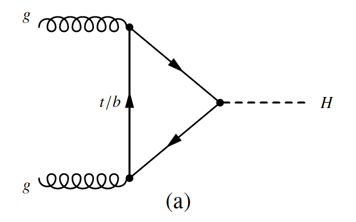
Figure 1-a:
Leading-order Feynman diagrams for Higgs boson production via the (a) ${gg\mathrm {F}}$ and (b) $ {V\mathrm {BF}}$ production processes. |
png ; pdf |
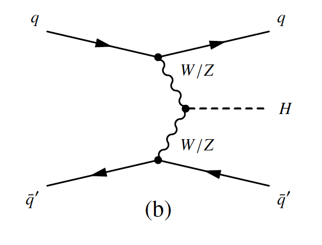
Figure 1-b:
Leading-order Feynman diagrams for Higgs boson production via the (a) ${gg\mathrm {F}}$ and (b) $ {V\mathrm {BF}}$ production processes. |
png ; pdf |
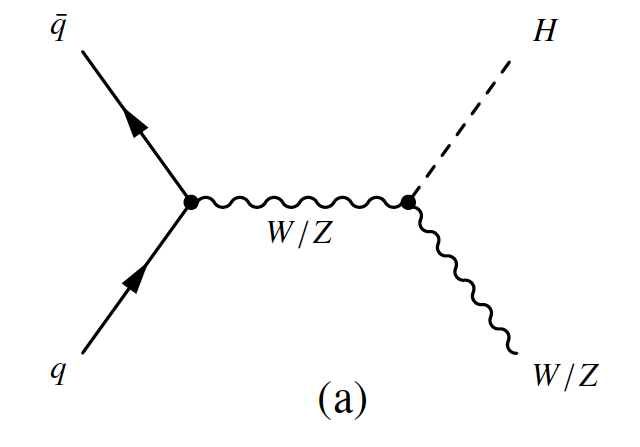
Figure 2-a:
Leading-order Feynman diagrams of Higgs boson production via the (a) $q\bar {q} \to VH$ and (b,c) $ {gg\to ZH}$ production processes. |
png ; pdf |
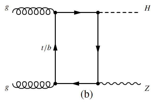
Figure 2-b:
Leading-order Feynman diagrams of Higgs boson production via the (a) $q\bar {q} \to VH$ and (b,c) $ {gg\to ZH}$ production processes. |
png ; pdf |
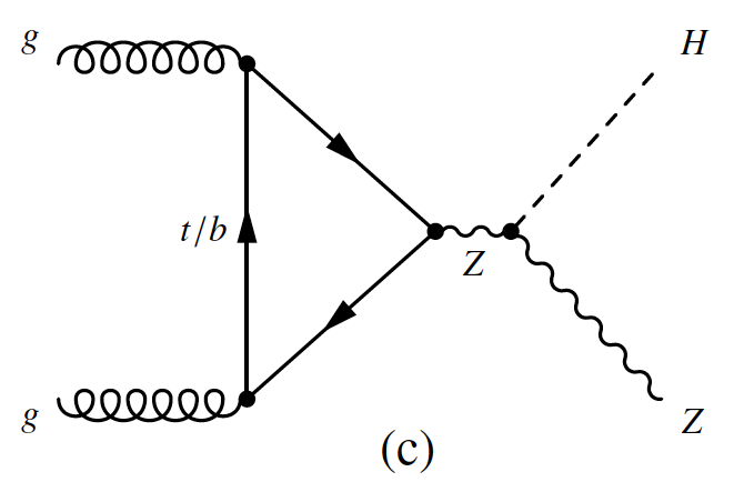
Figure 2-c:
Leading-order Feynman diagrams of Higgs boson production via the (a) $q\bar {q} \to VH$ and (b,c) $ {gg\to ZH}$ production processes. |
png ; pdf |
Figure 3-a:
Leading-order Feynman diagrams of Higgs boson production via the $ {q\bar {q}/gg \to t\bar {t}H}$ and $ {q\bar {q}/gg \to bbH}$ processes. |

png ; pdf |
Figure 3-b:
Leading-order Feynman diagrams of Higgs boson production via the $ {q\bar {q}/gg \to t\bar {t}H}$ and $ {q\bar {q}/gg \to bbH}$ processes. |

png ; pdf |
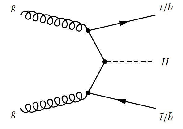
Figure 3-c:
Leading-order Feynman diagrams of Higgs boson production via the $ {q\bar {q}/gg \to t\bar {t}H}$ and $ {q\bar {q}/gg \to bbH}$ processes. |

png ; pdf |
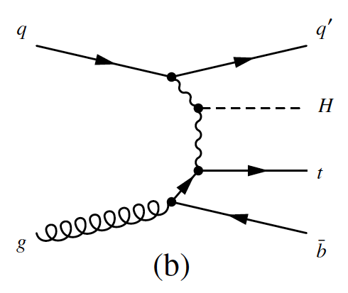
Figure 4-a:
Leading-order Feynman diagrams of the Higgs boson production in association with a single top quark: (a,b) $ {tHq}$ and (c,d) $ {tHW}$. |
png ; pdf |
Figure 4-b:
Leading-order Feynman diagrams of the Higgs boson production in association with a single top quark: (a,b) $ {tHq}$ and (c,d) $ {tHW}$. |
png ; pdf |
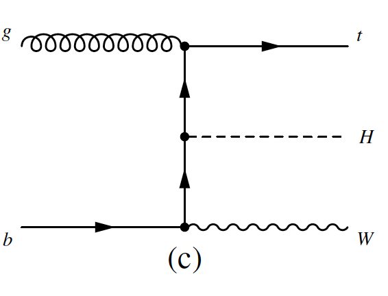
Figure 4-c:
Leading-order Feynman diagrams of the Higgs boson production in association with a single top quark: (a,b) $ {tHq}$ and (c,d) $ {tHW}$. |
png ; pdf |
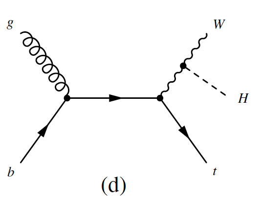
Figure 4-d:
Leading-order Feynman diagrams of the Higgs boson production in association with a single top quark: (a,b) $ {tHq}$ and (c,d) $ {tHW}$. |

png ; pdf |
Figure 5-a:
Leading-order Feynman diagrams of Higgs boson decays (a) to $W$ and $Z$ bosons and (b) to fermions. |
png ; pdf |
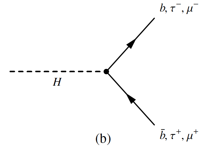
Figure 5-b:
Leading-order Feynman diagrams of Higgs boson decays (a) to $W$ and $Z$ bosons and (b) to fermions. |
png ; pdf |
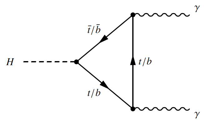
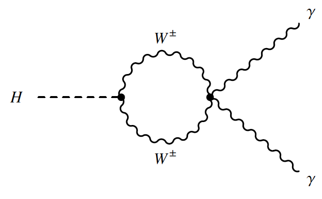
Figure 6-a:
Leading-order Feynman diagrams of Higgs boson decays to a pair of photons. |
png ; pdf |
Figure 6-b:
Leading-order Feynman diagrams of Higgs boson decays to a pair of photons. |
png ; pdf |
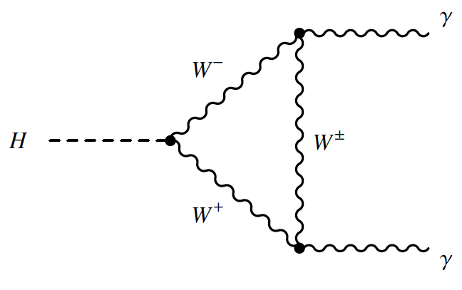
Figure 6-c:
Leading-order Feynman diagrams of Higgs boson decays to a pair of photons. |
png ; pdf |
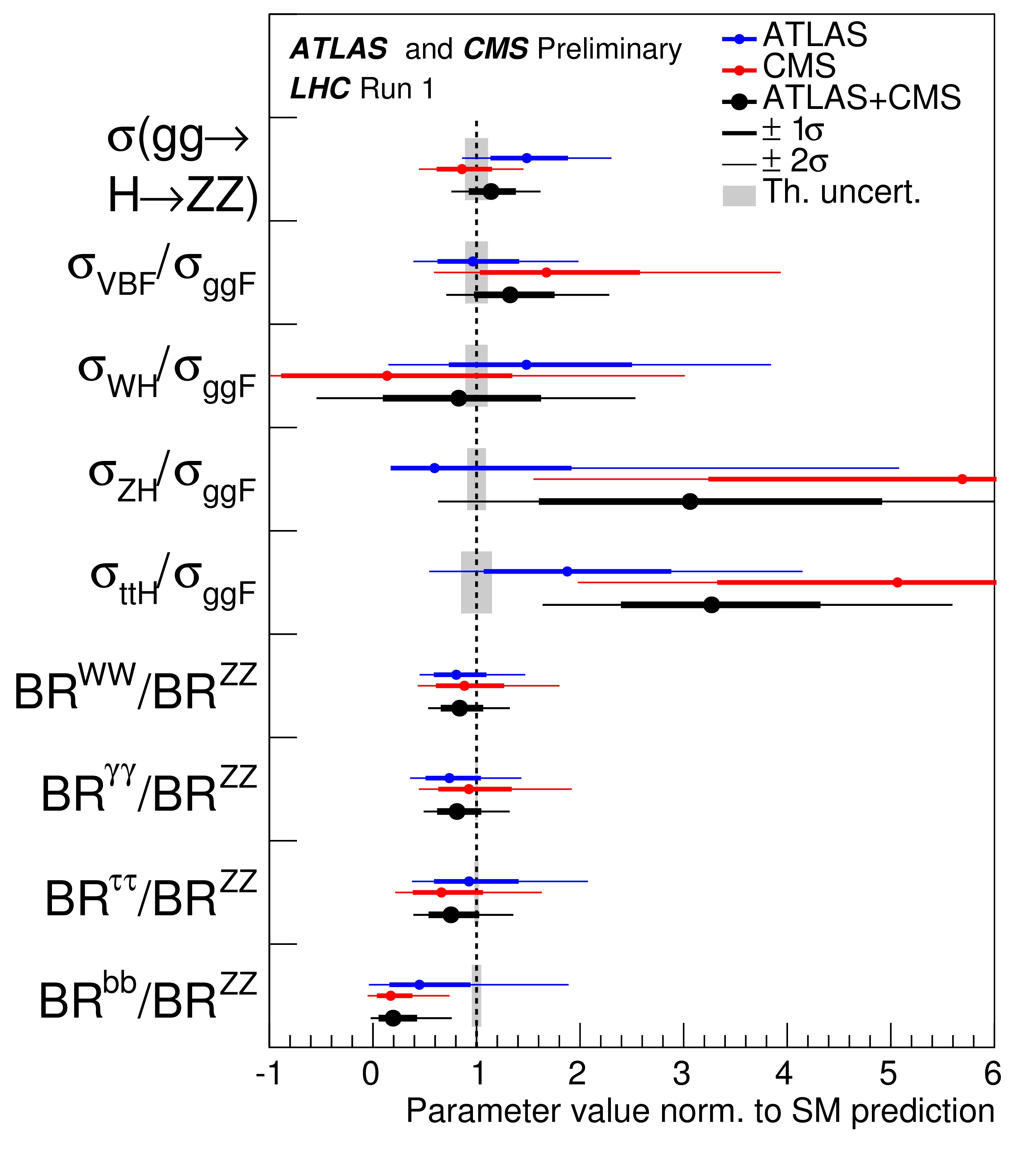
Figure 7:
Best-fit values of the $\sigma (gg \to H \to ZZ)$ cross section and of ratios of cross sections and branching ratios, as obtained from the generic parameterisation described in the text and as tabulated in Table 7 for the combination of ATLAS and CMS measurements. Also shown for completeness are the results for each experiment. The error bars indicate the $1\sigma $ (thick lines) and $2\sigma $ (thin lines) intervals. In this figure, the fit results are normalised to the SM predictions for the various parameters and the shaded bands indicate the theory uncertainties on these predictions. |
png ; pdf |
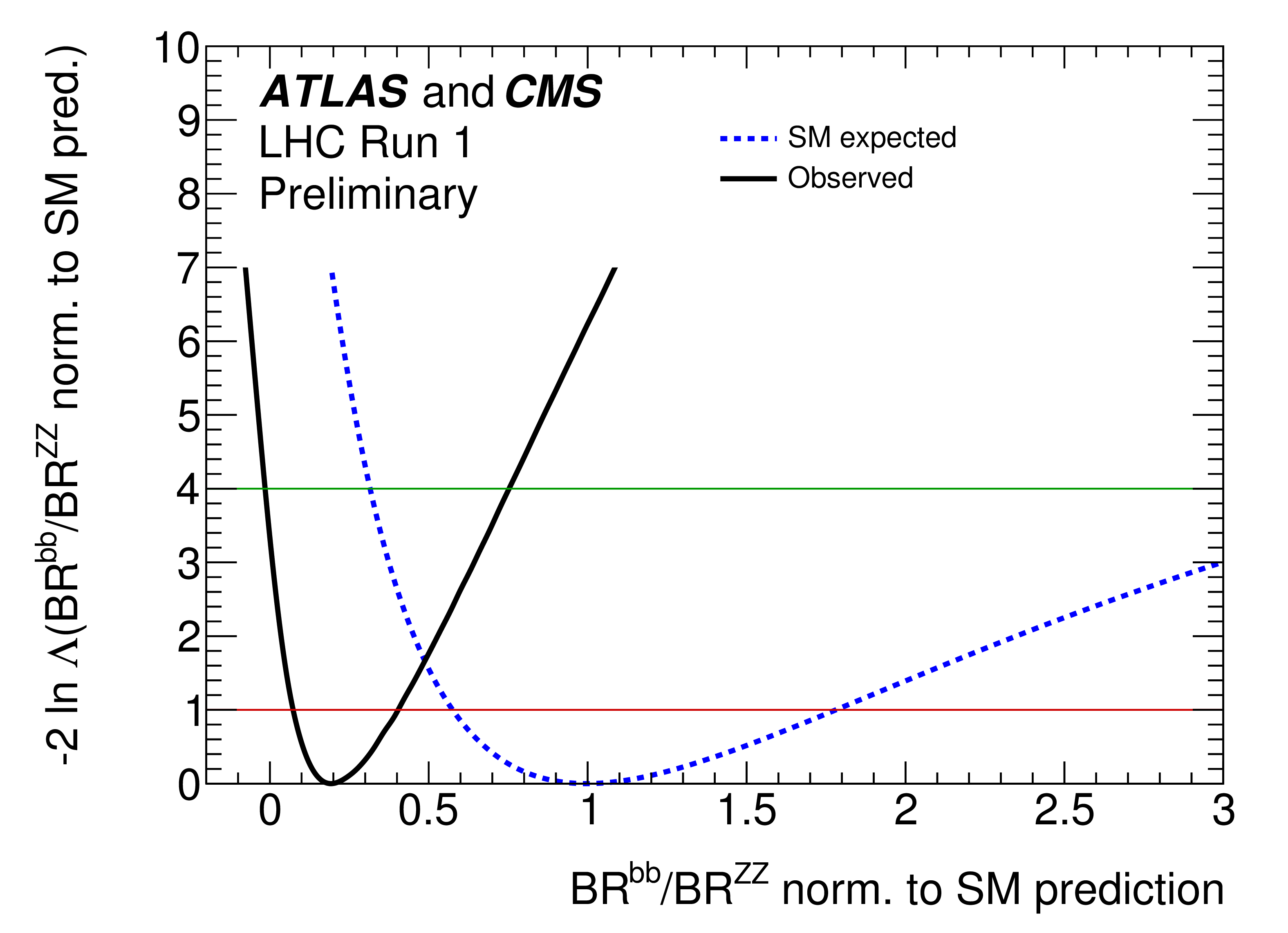
Figure 8:
Observed (solid line) and expected (dashed line) negative log-likelihood scan of the $\mathrm {BR}^{bb}/\mathrm {BR}^{ZZ}$ parameter. All the other ratios of cross sections and branching ratios in the parameterisation are profiled. The red (green) horizontal line indicates the value of the profile likelihood ratio corresponding to a $1\sigma $ ($2\sigma $) confidence interval for the parameter of interest, assuming the asymptotic $\chi ^2$ distribution for the test statistic. |

png ; pdf |
Figure 9:
Best-fit values of ratios of Higgs boson coupling modifiers, as obtained from the generic parameterisation described in the text and as tabulated in Table 8 for the combination of ATLAS and CMS measurements. Also shown for completeness are the results for each experiment. The error bars indicate the $1\sigma $ (thick lines) and $2\sigma $ (thin lines) intervals. The hatched areas indicate the parameters which are assumed to be positive without loss of generality. |

png ; pdf |
Figure 10-a:
Negative log-likelihood scans for $ {\lambda }_{W Z }$ and $ {\lambda }_{t g}$, the two parameters of Fig. 9 which are of interest in the negative range in the the generic parameterisation of ratios of Higgs boson coupling modifiers described in the text. |
png ; pdf |
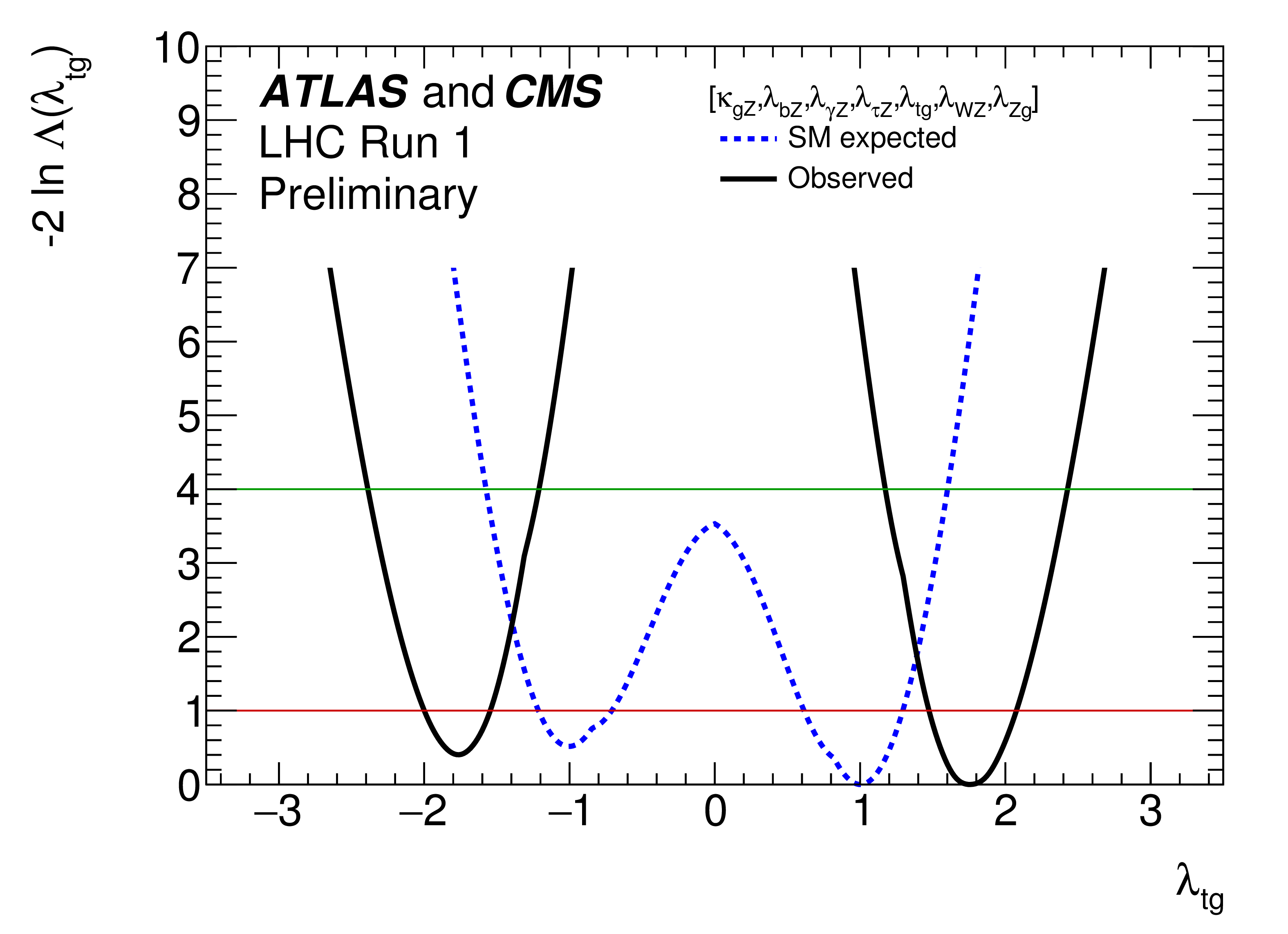
Figure 10-b:
Negative log-likelihood scans for $ {\lambda }_{W Z }$ and $ {\lambda }_{t g}$, the two parameters of Fig. 9 which are of interest in the negative range in the the generic parameterisation of ratios of Higgs boson coupling modifiers described in the text. |
png ; pdf |
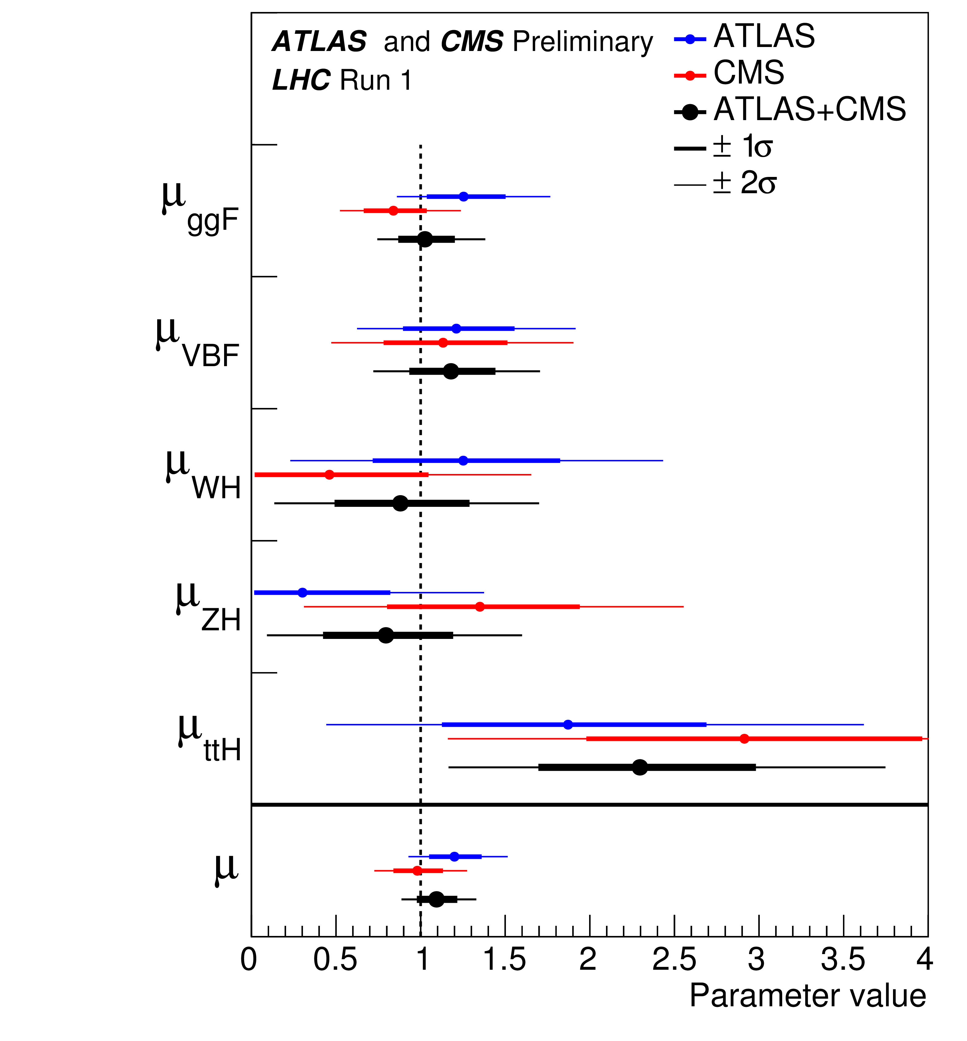
Figure 11:
Best-fit results for the production signal strengths for the combination of ATLAS and CMS. Also shown for completeness are the results for each experiment. The error bars indicate the $1\sigma $ (thick lines) and $2\sigma $ (thin lines) intervals. The measurements of the global signal strength $\mu $ are also shown. |
png ; pdf |
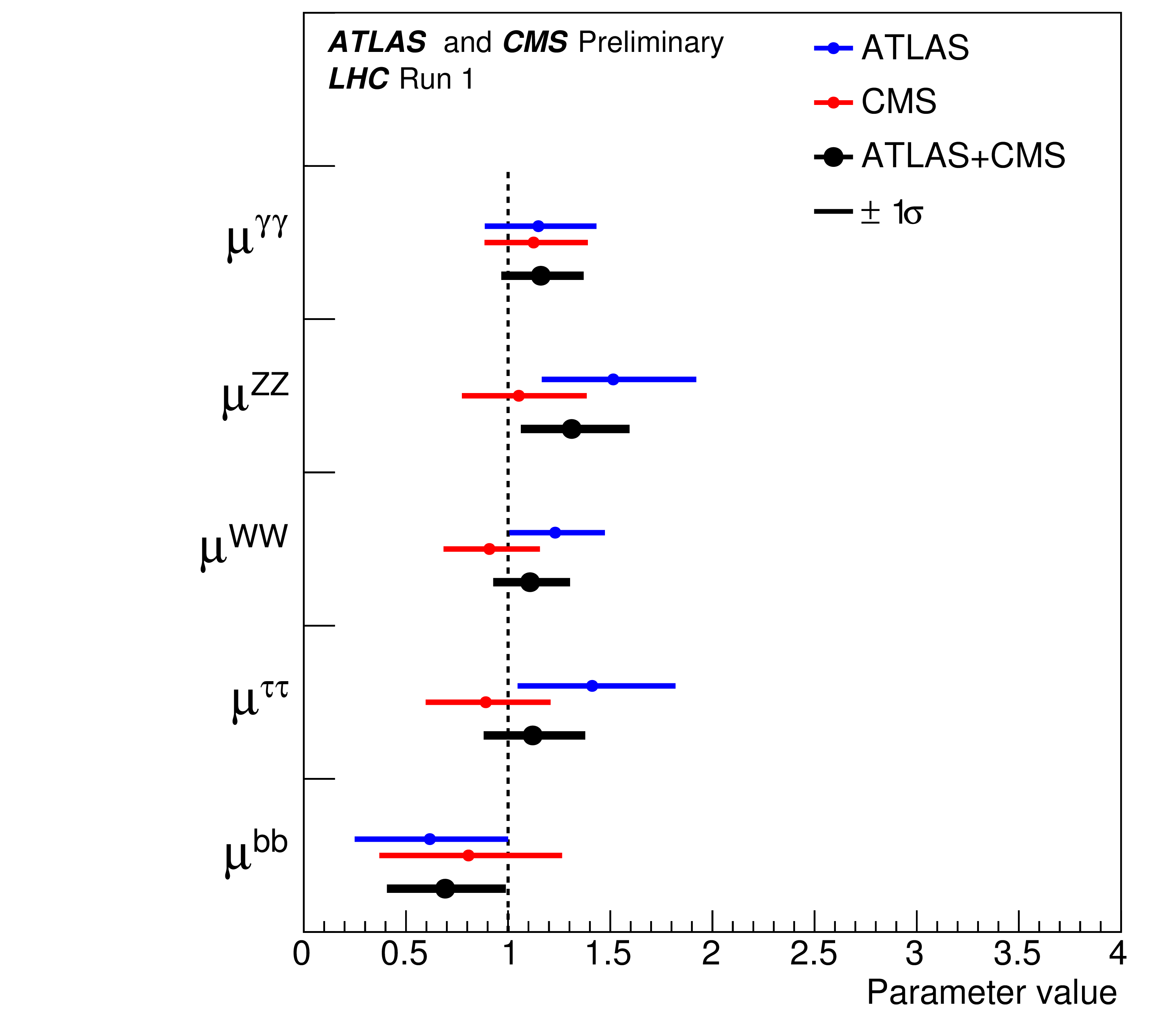
Figure 12:
Best-fit results for the decay signal strengths for the combination of ATLAS and CMS. Also shown for completeness are the results for each experiment. The error bars indicate the $1\sigma $ intervals. |
png ; pdf |
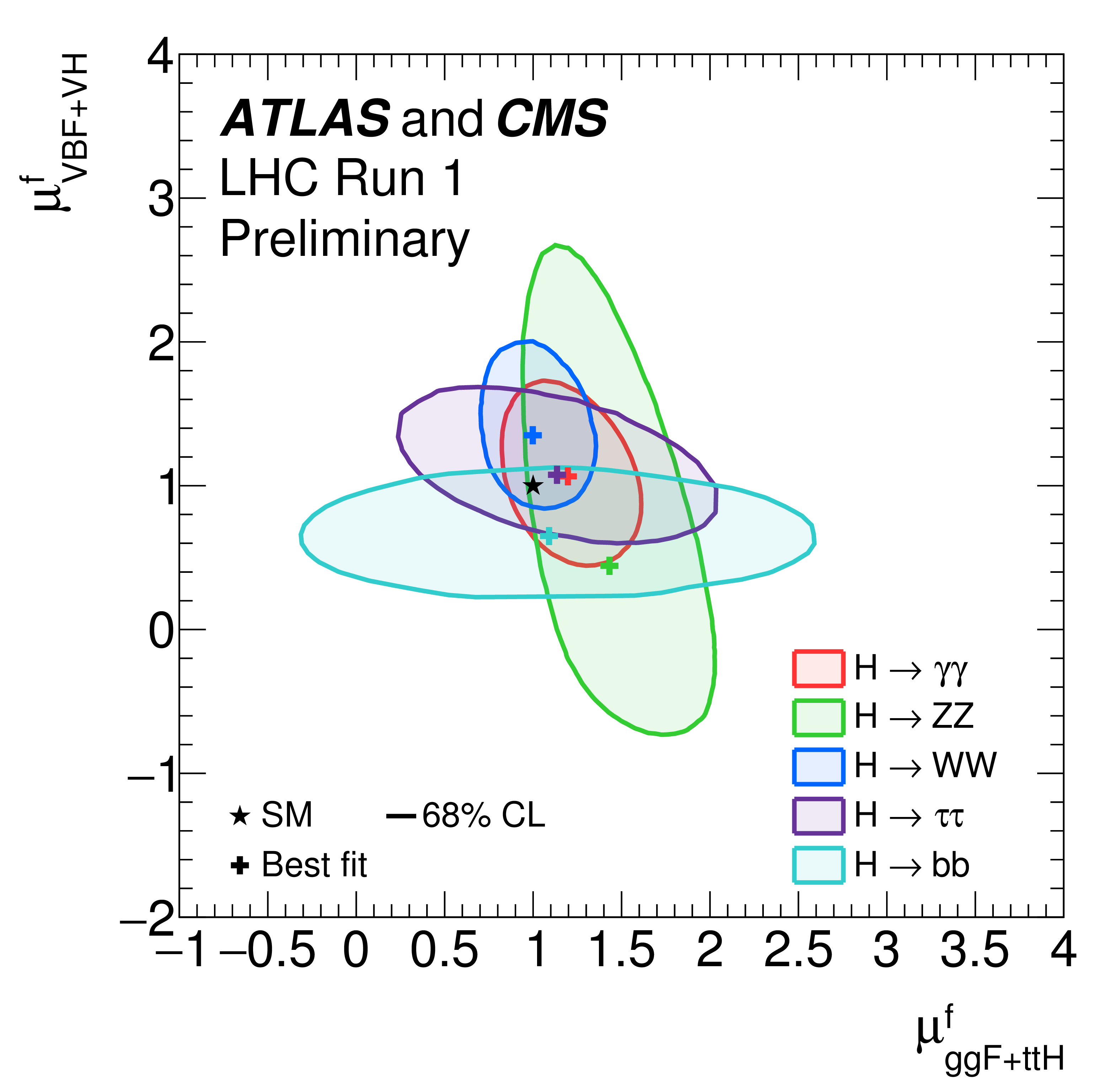
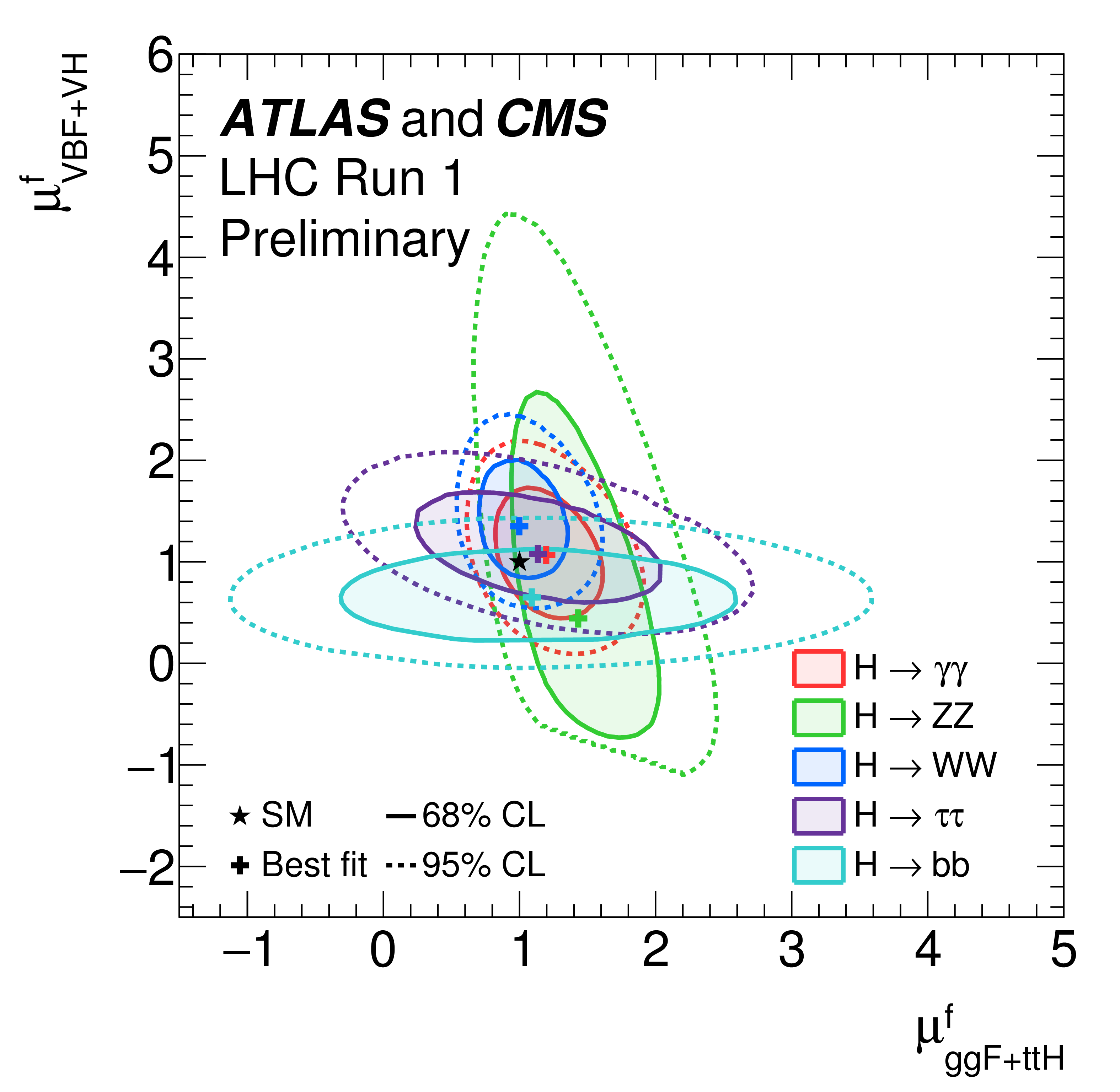
Figure 13:
Likelihood contours in the ($\mu _{ {gg\mathrm {F}}+ {ttH}}^f$, $\mu _{ {V\mathrm {BF}}+ {VH}}^f$) plane for the combination of ATLAS and CMS, shown for the five decay channels, $ {H \to ZZ}$, $H \to WW$, $ {H \to \gamma \gamma }$, $H \to \tau \tau $, and $H \to bb$. The results are shown as 68% CL contours, together with the best-fit values to the data and the SM~expectation. Figure 28 in Appendix C shows both the 68% and 95% contours for the results of these fits. |
png ; pdf |
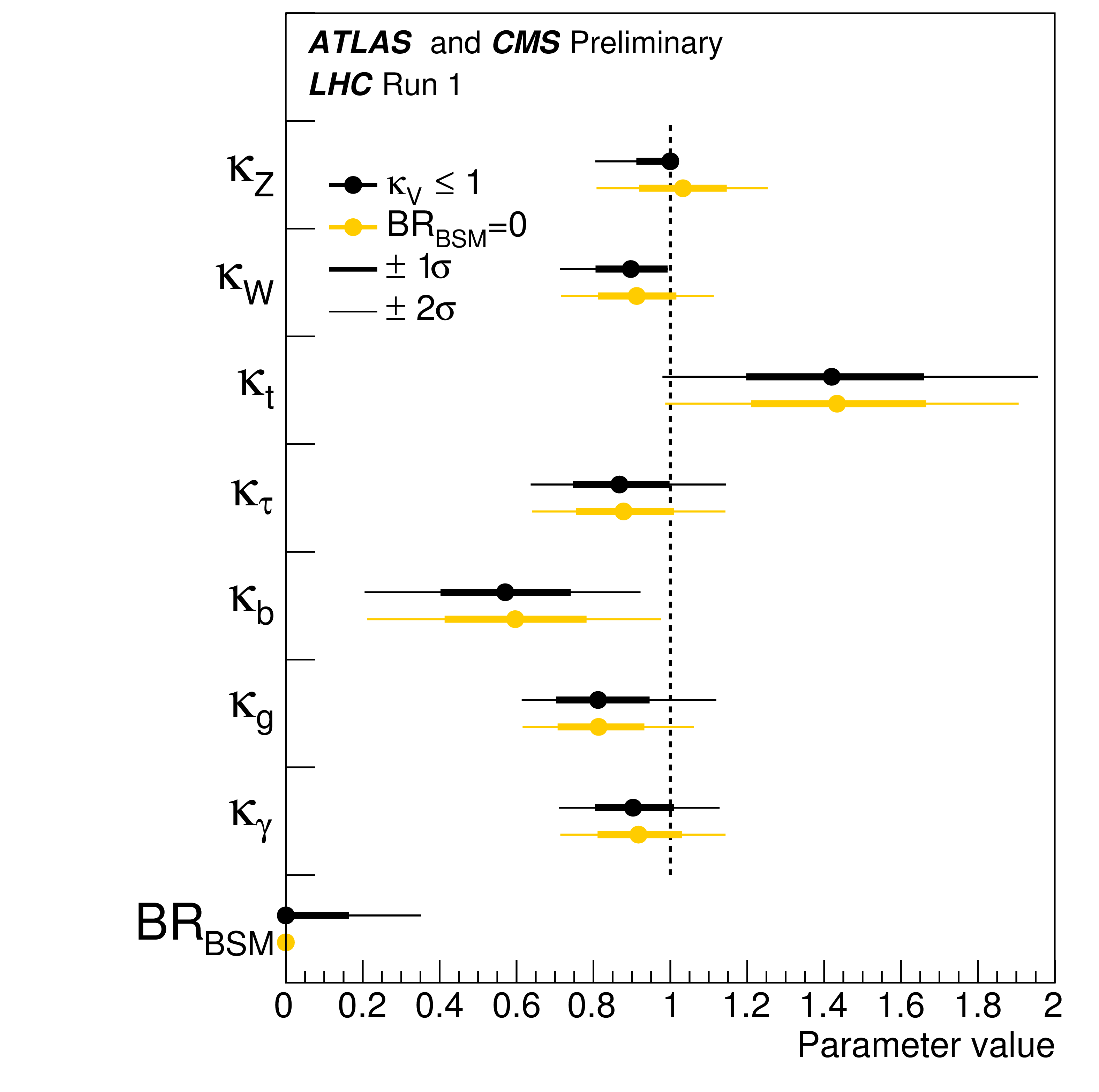
Figure 14:
Fit results for the two parameterisations allowing BSM loop couplings, with $ {\kappa }_{V} \le 1$, where $ {\kappa }_{V}$ stands for $ {\kappa }_{Z}$ or $ {\kappa }_{W}$, or without additional BSM contributions to the Higgs boson width, i.e. $ {\mathrm {BR_{BSM}}}=0$. The measured results for the combination of ATLAS and CMS are reported together with their uncertainties. The error bars indicate the $1\sigma $ (thick lines) and $2\sigma $ (thin lines) intervals. The uncertainties are not indicated when the parameters are constrained and hit a boundary, namely $ {\kappa }_{V} = 1$ or $ {\mathrm {BR_{BSM}}}= 0$. |
png ; pdf |
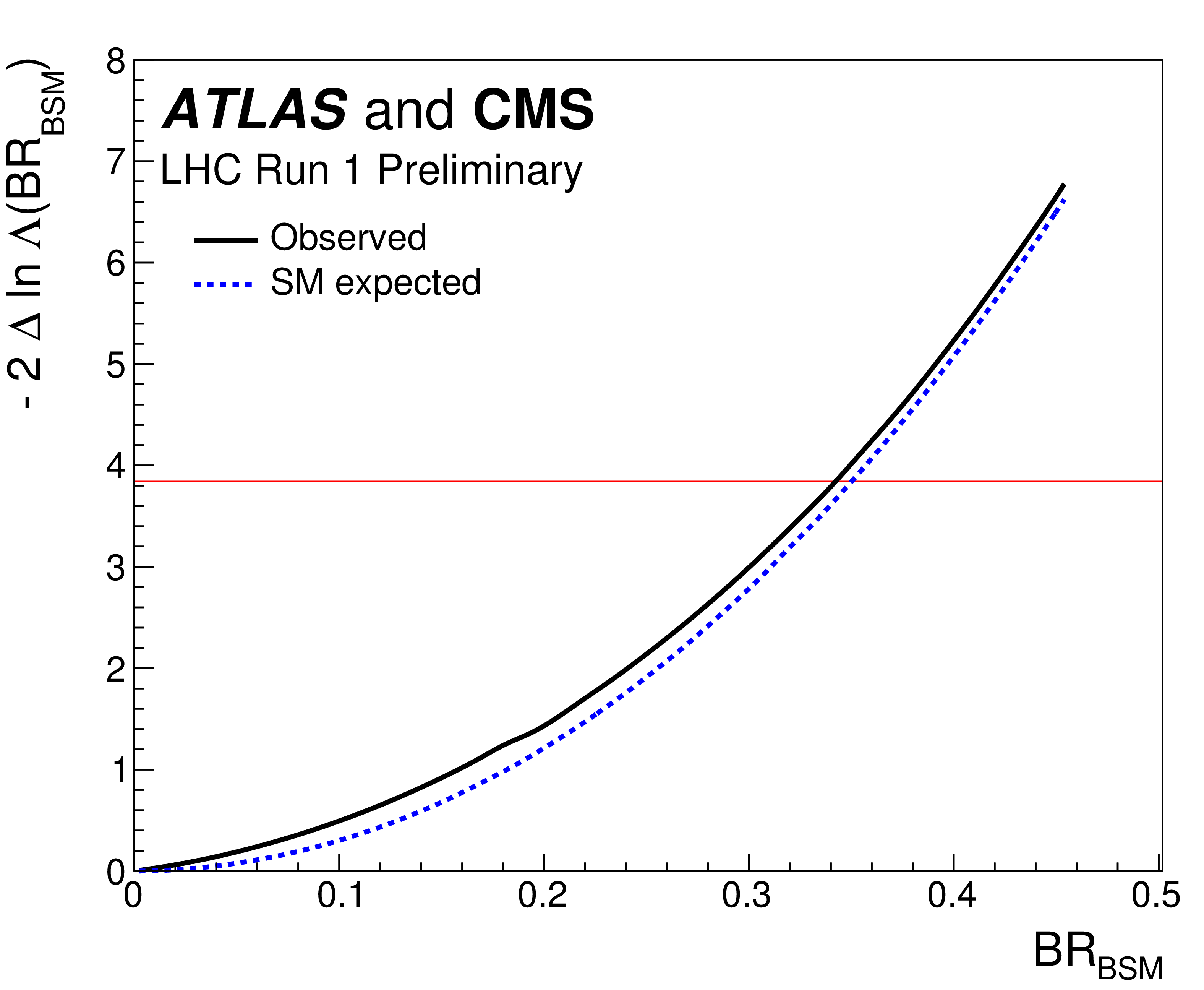
Figure 15:
Observed and expected negative log-likelihood scan of $ {\mathrm {BR_{BSM}}}$, shown for the combination of ATLAS and CMS in the case of the parameterisation allowing non-SM loop couplings with additional BSM contributions to the Higgs boson width. This corresponds to the constraint $ {\kappa }_{V}\le 1$ in Fig.14. The red horizontal line at 3.84 indicates the log-likelihood variation corresponding to the 95% CL upper limit, as discussed in Section 3.2. |
png ; pdf |
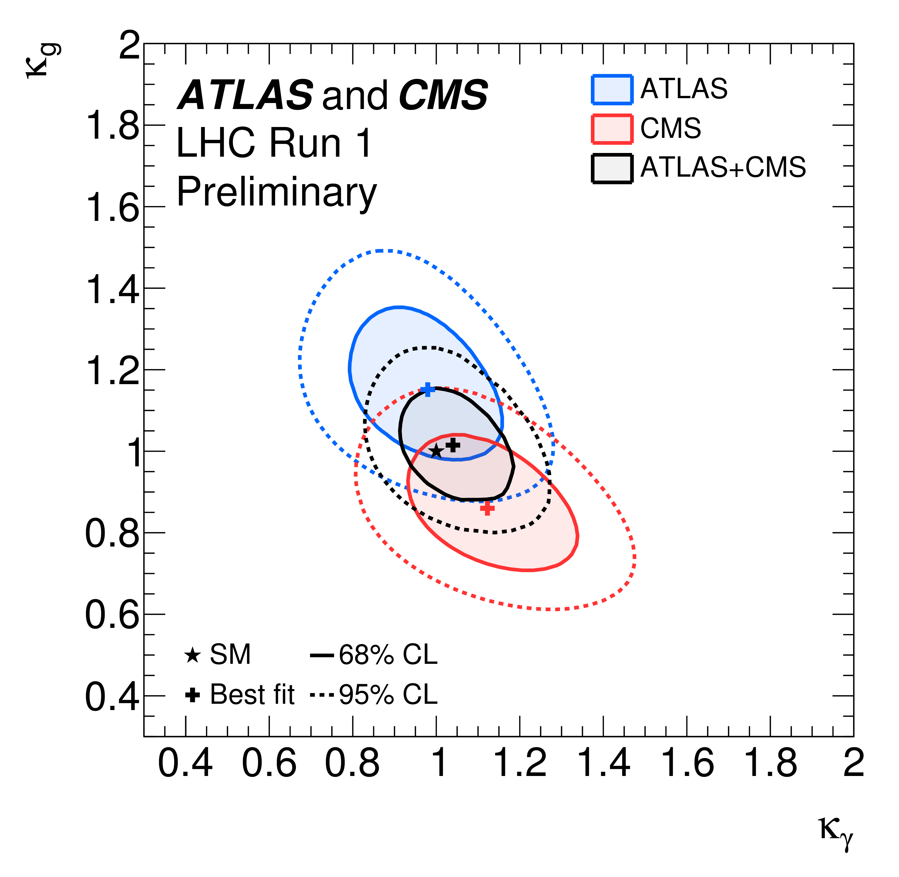
Figure 16:
Negative log-likelihood contours at 68% and 95% CL of $ {\kappa _\gamma }$ versus $ {\kappa _g}$ for the combination of ATLAS and CMS and for each experiment separately, for the parameterisation constraining all the other coupling modifiers to their SM values and assuming $ {\mathrm {BR_{BSM}}}= 0$. |
png ; pdf |
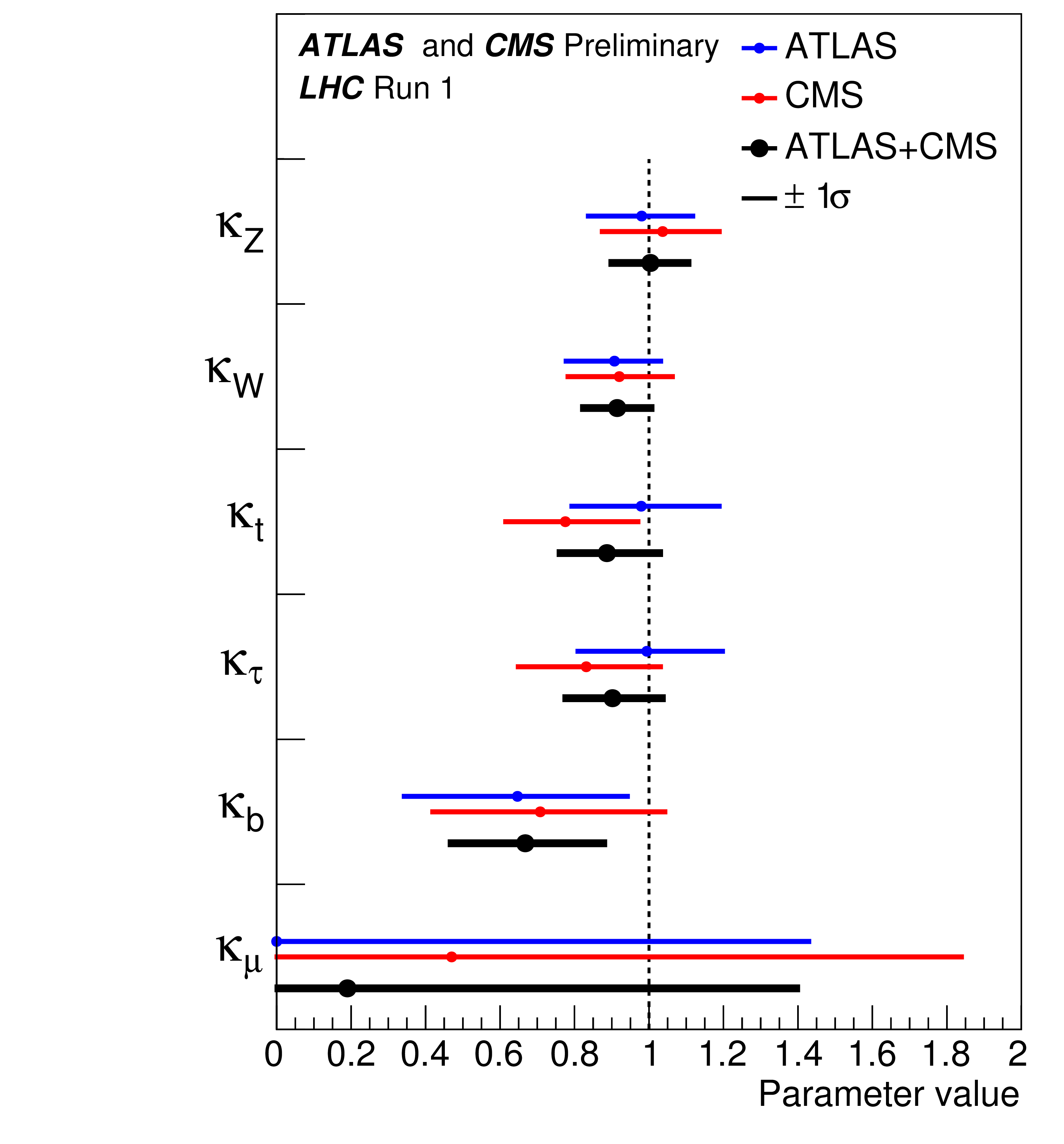
Figure 17:
Best-fit values of parameters for the combination of ATLAS and CMS and separately for each experiment, for the parameterisation assuming the absence of BSM particles in the loops, $ {\mathrm {BR_{BSM}}}=0$, and $\kappa _j \ge 0$. The uncertainties are not indicated when the parameters are constrained and hit a boundary, namely $\kappa _j = 0$. |
png ; pdf |
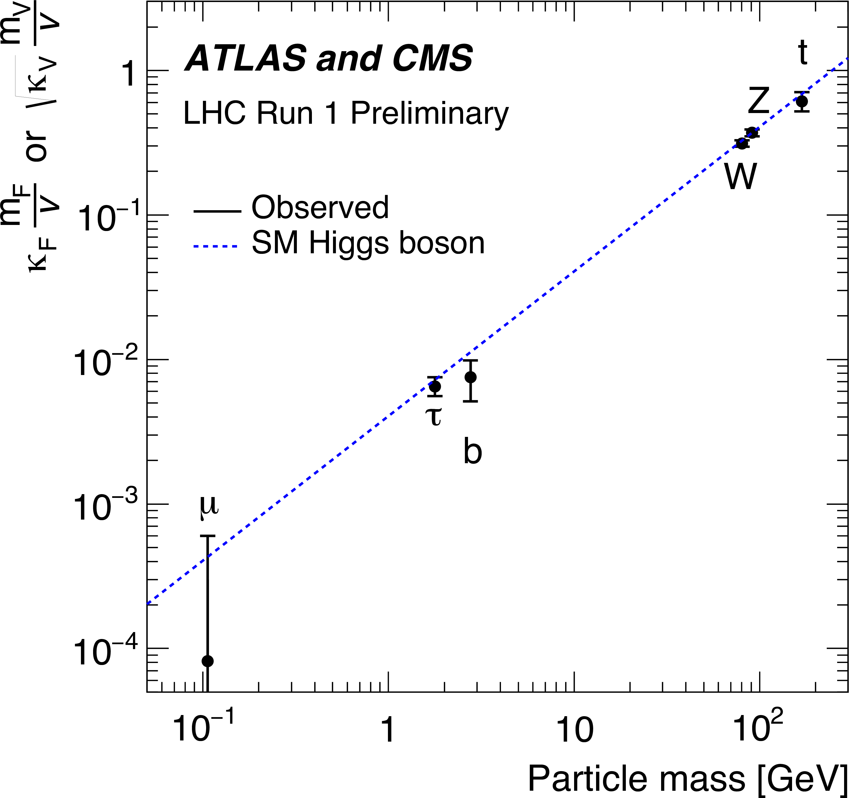
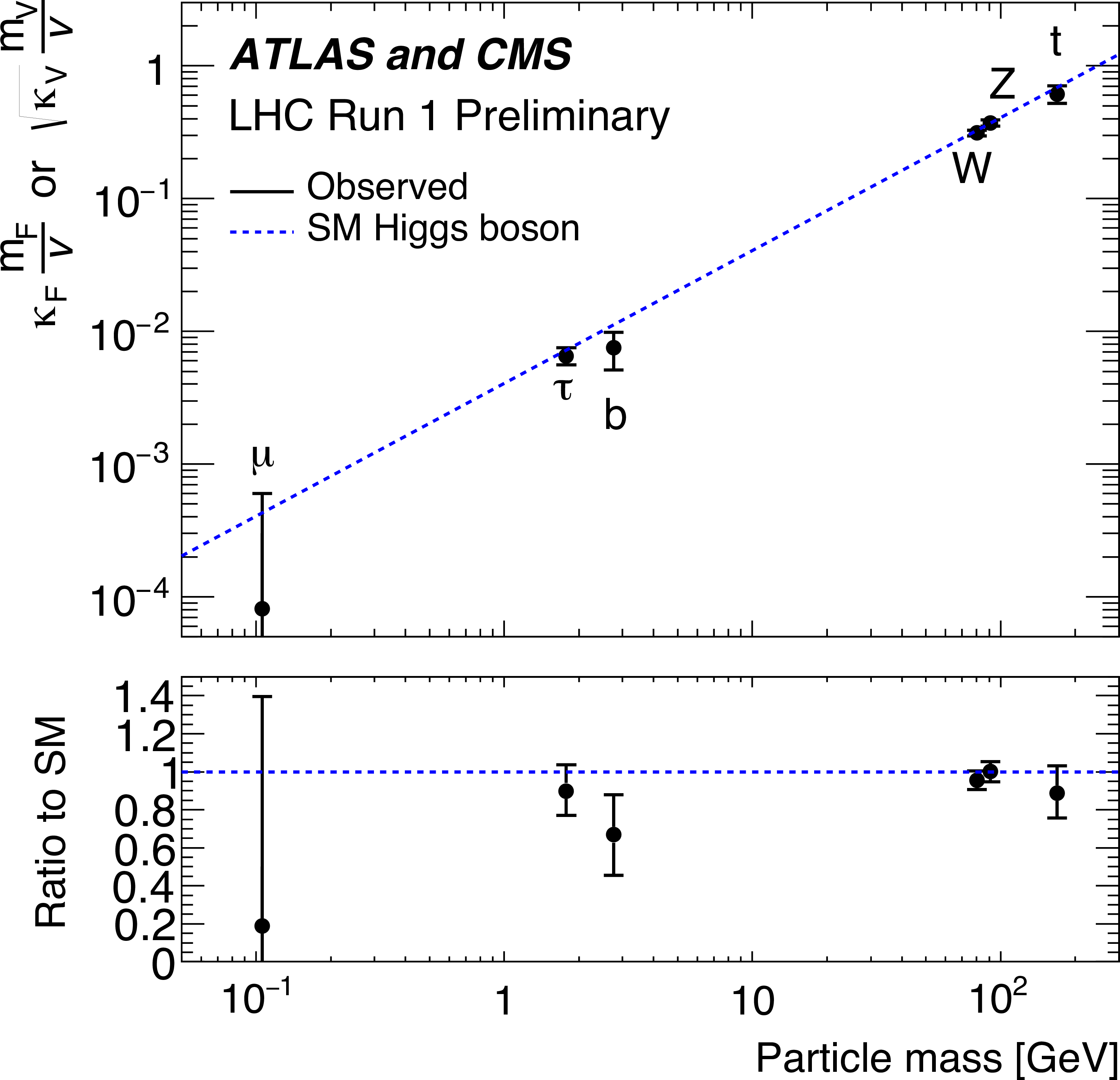
Figure 18:
Fit results for the combination of ATLAS and CMS in the case of the parameterisation with reduced coupling modifiers $y_{V,i} = \sqrt { {\kappa }_{V,i} \frac {g_{V,i}}{2v} } = \sqrt { {\kappa }_{V,i}}\frac {m_{V,i}}{v}$ for the weak vector bosons, and $y_{F,i} = {\kappa }_{F,i}\frac {g_{F,i}}{\sqrt {2}} = {\kappa }_{F,i}\frac {m_{F,i}}{v}$ for the fermions, as a function of the particle mass. The dashed line indicates the predicted dependence on the particle mass for the SM Higgs boson. |
png ; pdf |
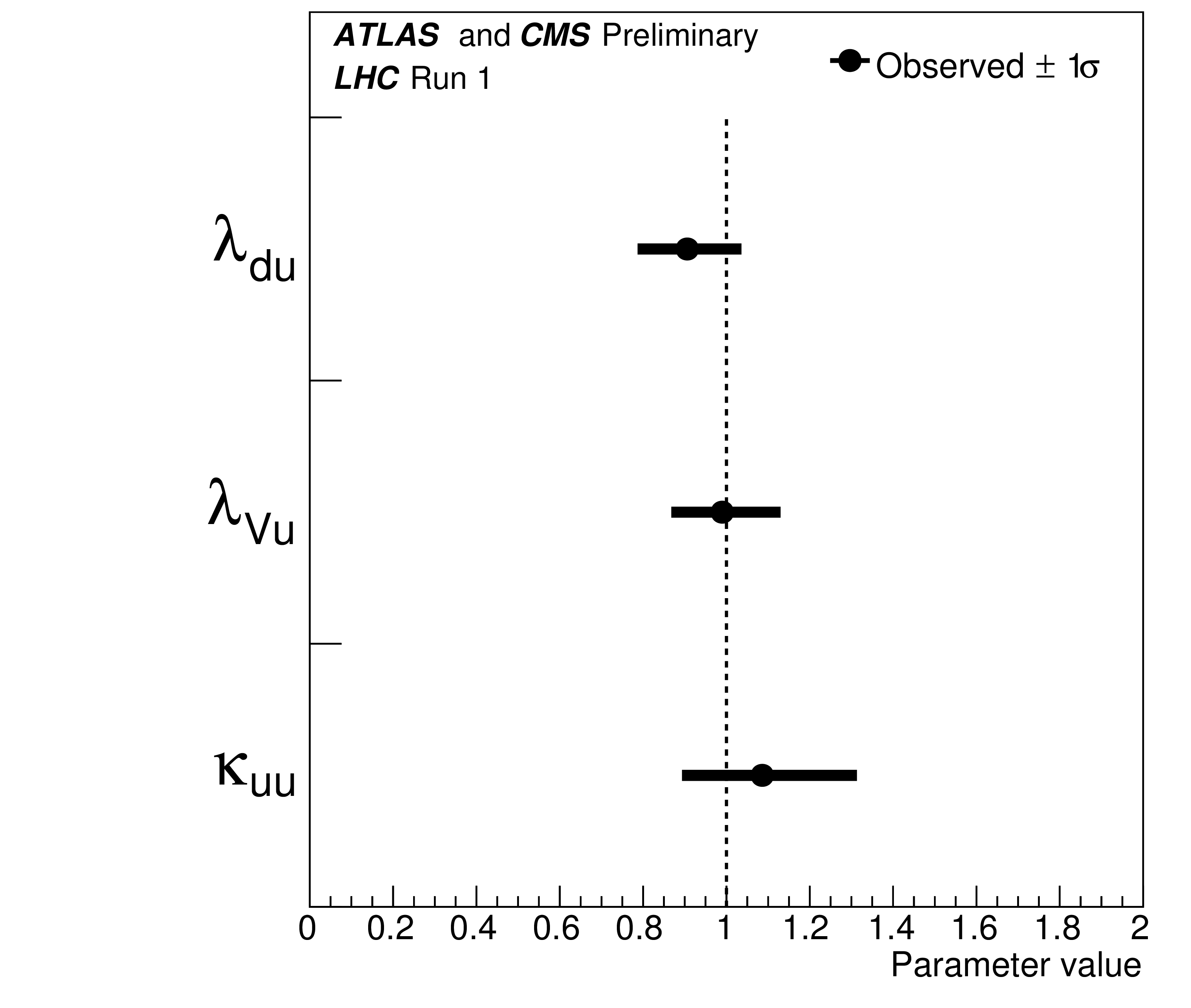
Figure 19:
$1\sigma $ intervals for combined results of the $\lambda _{du}$, $\lambda _{Vu}$ and $\kappa _{uu}$ parameters from fits with the most general parameterisation testing the up- and down-fermion coupling ratios. The negative range for $\lambda _{du}$ is not shown because no values are allowed in the 68% CL interval, as can be seen in Fig. 20. |
png ; pdf |
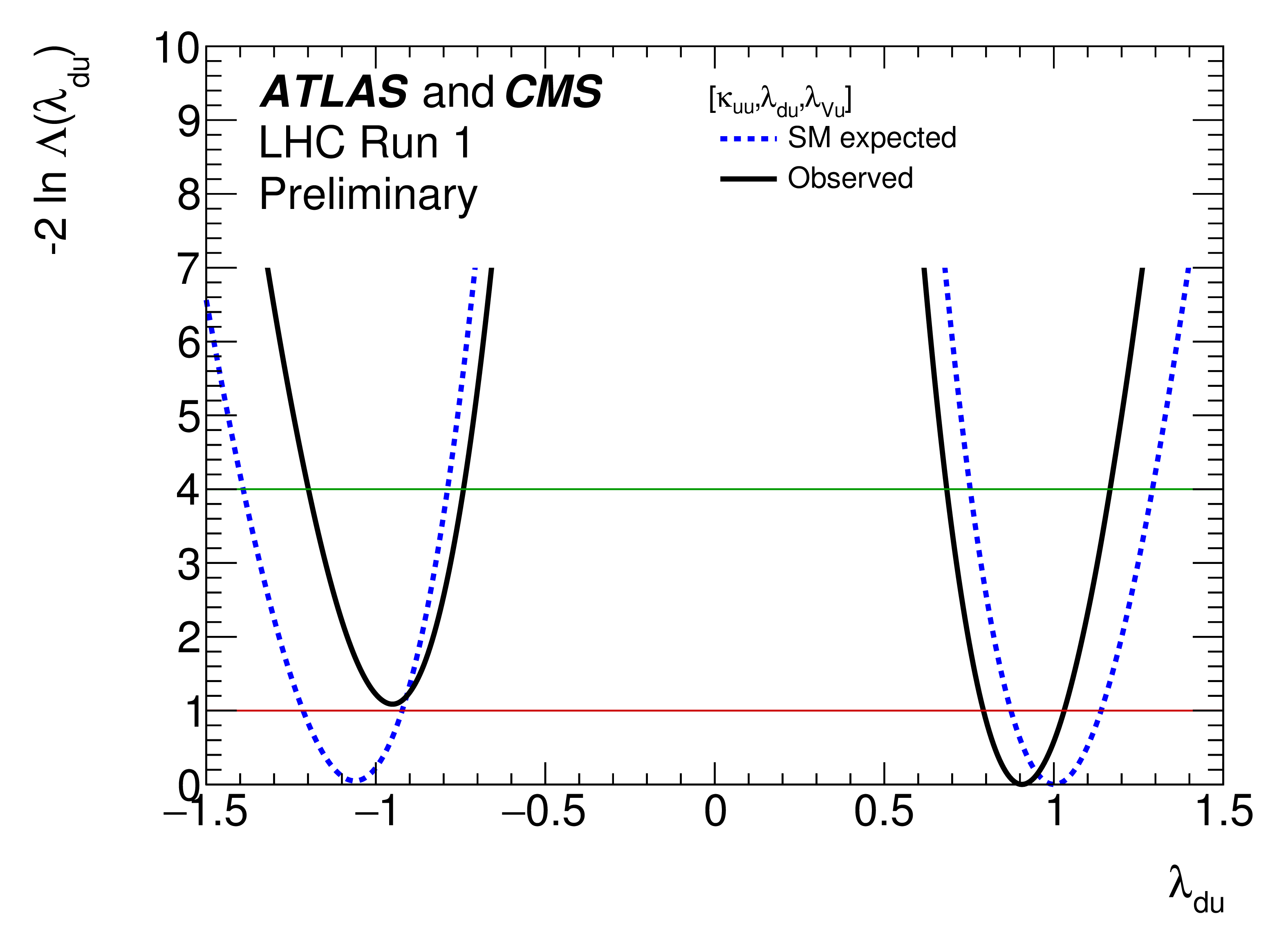
Figure 20:
Negative log-likelihood scan of the $\lambda _{du}$ parameter, probing the ratios of coupling modifiers for up-type versus down-type fermions for the combination of ATLAS and CMS, while profiling the other two parameters $\lambda _{Vu}$ and $\kappa _{uu}$. Both observed (solid) and expected (dotted) curves are shown. |
png ; pdf |
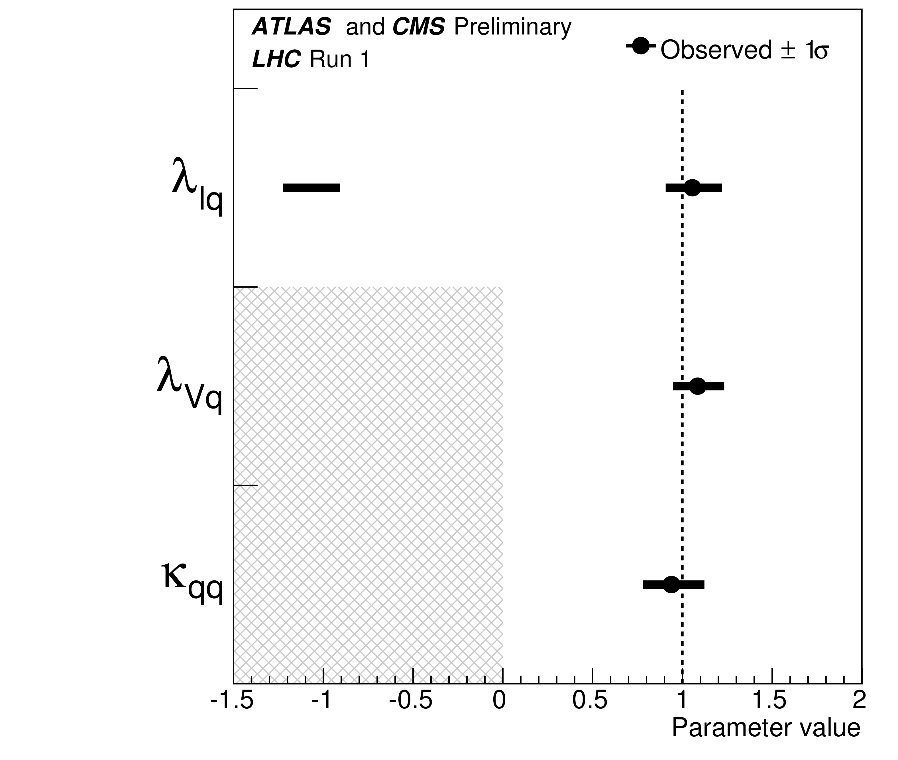
Figure 21:
$1\sigma $ intervals for combined results of the $\lambda _{lq}$, $\lambda _{Vq}$ and $\kappa _{qq}$ parameters from fits with the most general parameterisation testing the lepton and quark coupling ratios. The hatched areas indicate the parameters which are assumed to be positive without loss of generality. |
png ; pdf |
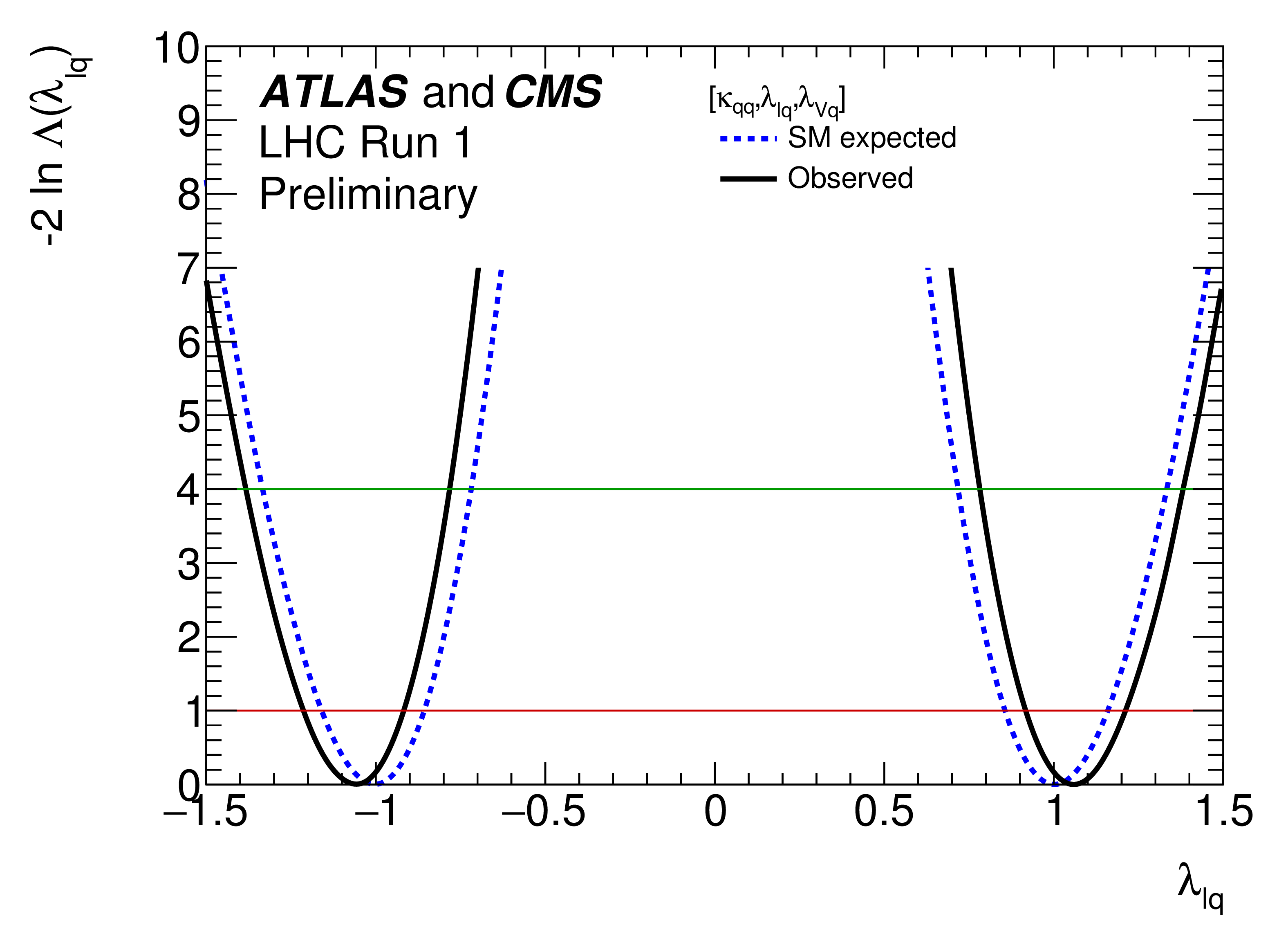
Figure 22:
Negative log-likelihood scan of the $\lambda _{lq}$ parameter, profiling the other two parameters $\lambda _{Vq}$ and $\kappa _{qq}$. Both observed (solid) and expected (dotted) curves are shown. |

png ; pdf |
Figure 23-a:
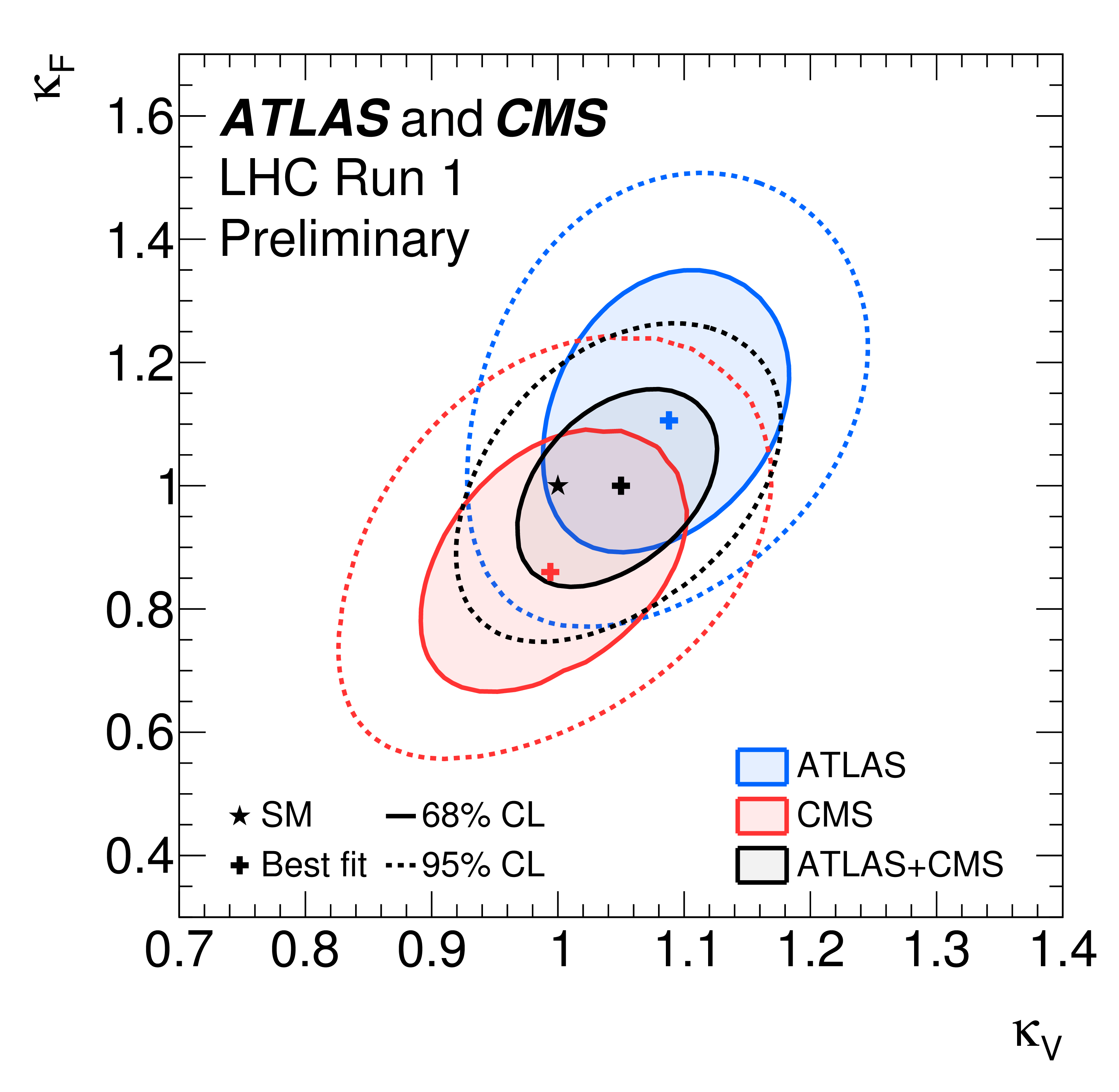
a: negative log-likelihood contours of $\kappa _F^f$ versus $\kappa _V^f$ for the combination of ATLAS and CMS and for the individual decay channels as well as for their global combination ($\kappa _F$ versus $\kappa _V$ shown in black), assuming that all coupling modifiers are positive. b: negative log-likelihood contours of $\kappa _F$ versus $\kappa _V$ on an enlarged scale for the combination of ATLAS and CMS and for the global fit of all channels. Also shown are the contours obtained for each experiment. |
png ; pdf |
Figure 23-b:
a: negative log-likelihood contours of $\kappa _F^f$ versus $\kappa _V^f$ for the combination of ATLAS and CMS and for the individual decay channels as well as for their global combination ($\kappa _F$ versus $\kappa _V$ shown in black), assuming that all coupling modifiers are positive. b: negative log-likelihood contours of $\kappa _F$ versus $\kappa _V$ on an enlarged scale for the combination of ATLAS and CMS and for the global fit of all channels. Also shown are the contours obtained for each experiment. |
png ; pdf |
Figure 24:
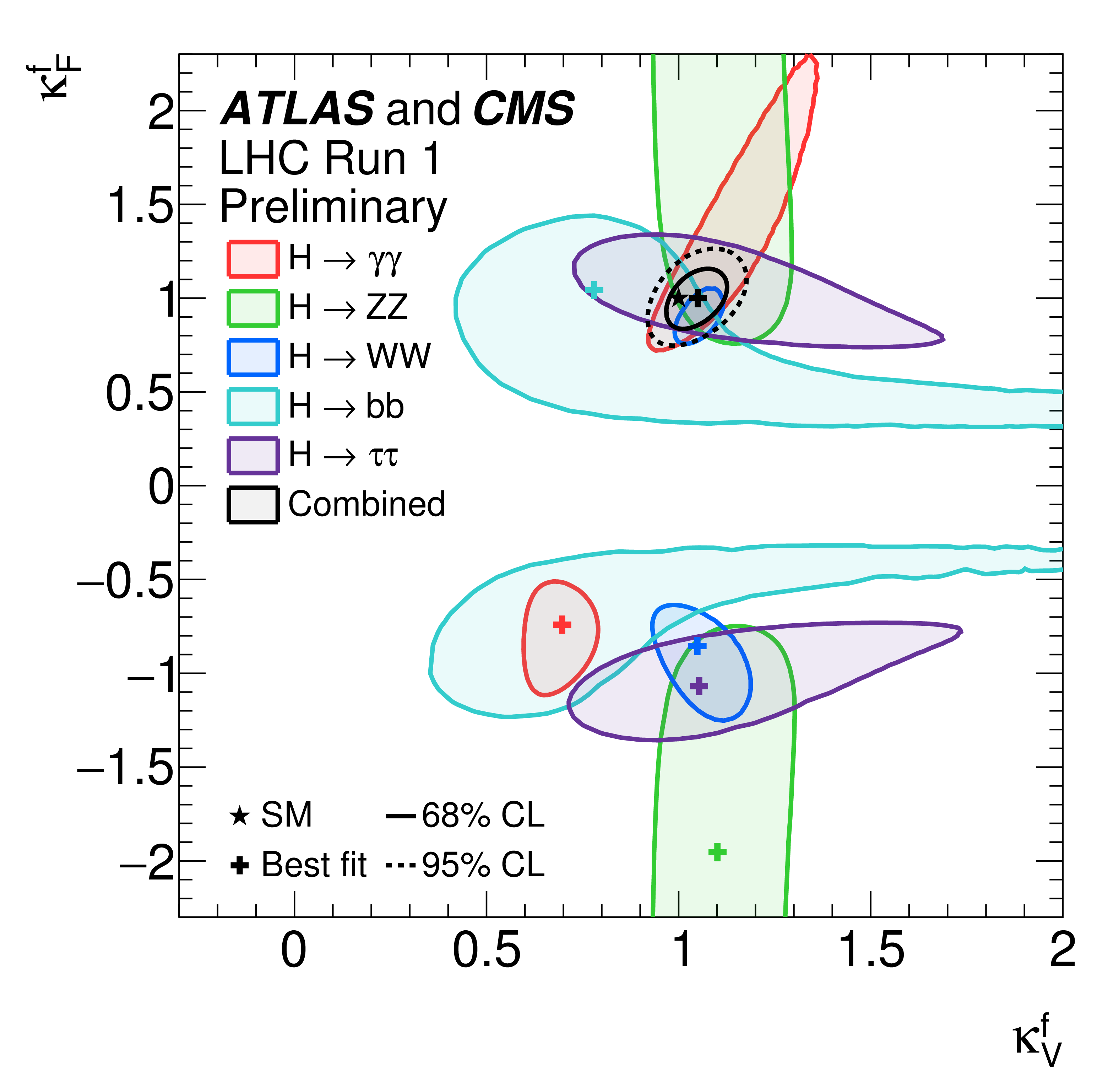
Negative log-likelihood contours of $\kappa _F^f$ versus $\kappa _V^f$ for the combination of ATLAS and CMS and for the individual decay channels, as well as for their global combination ($\kappa _F$ versus $\kappa _V$ shown in black), without any assumptions on the sign of the coupling modifiers. The other two quadrants (not shown) are symmetric with respect to the point (0,0). |
png ; pdf |
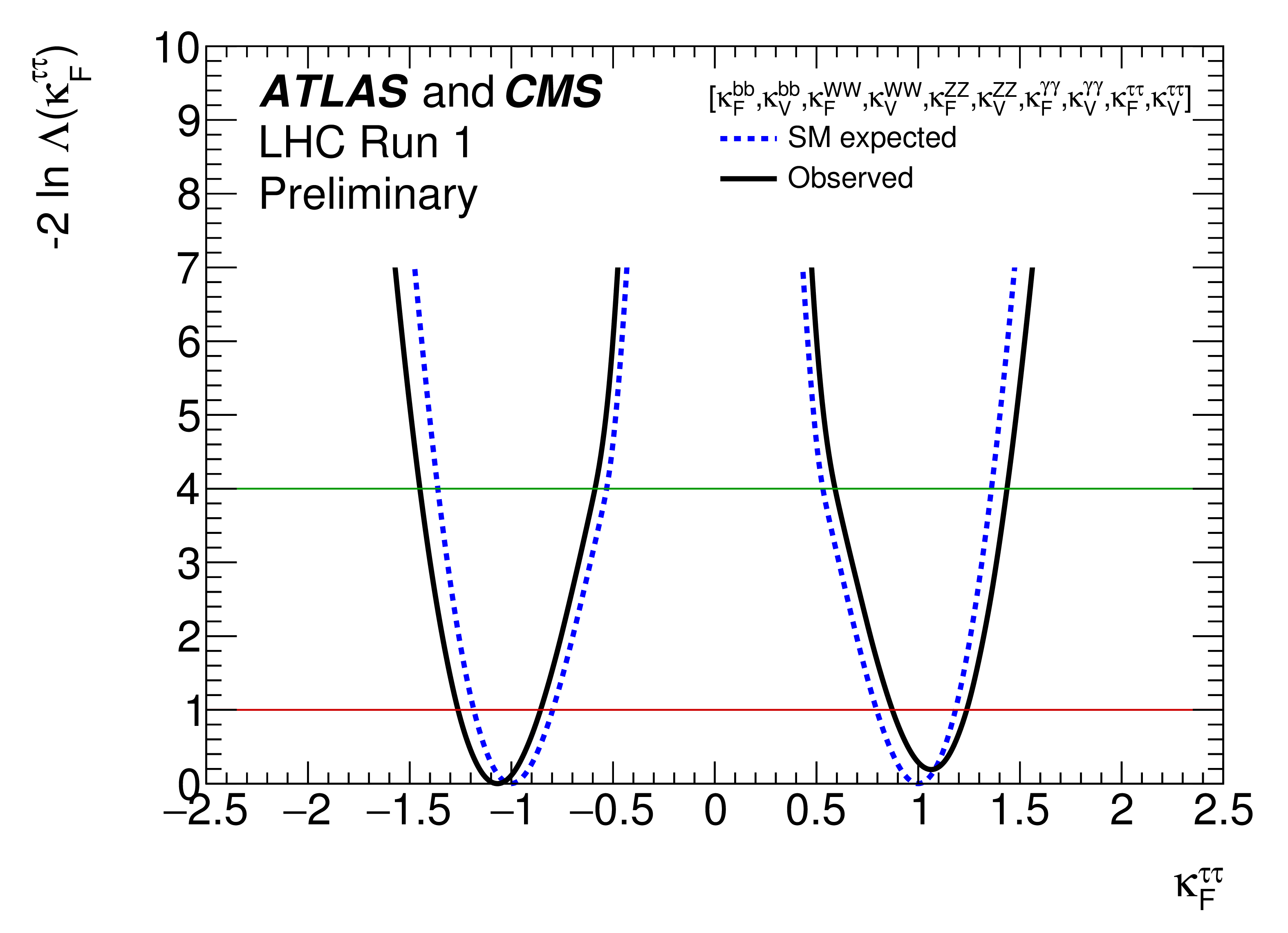
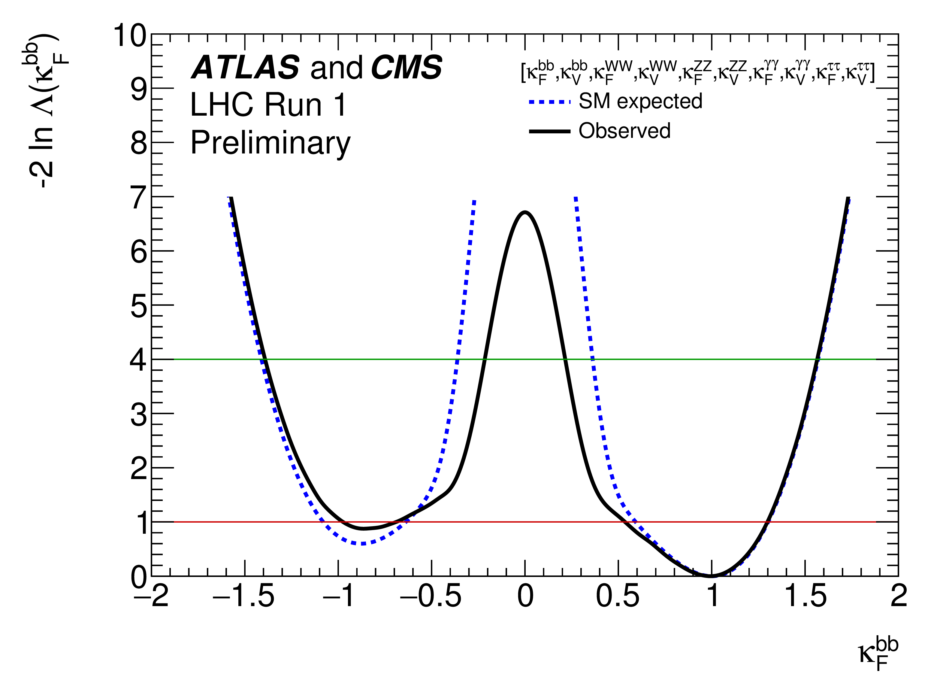
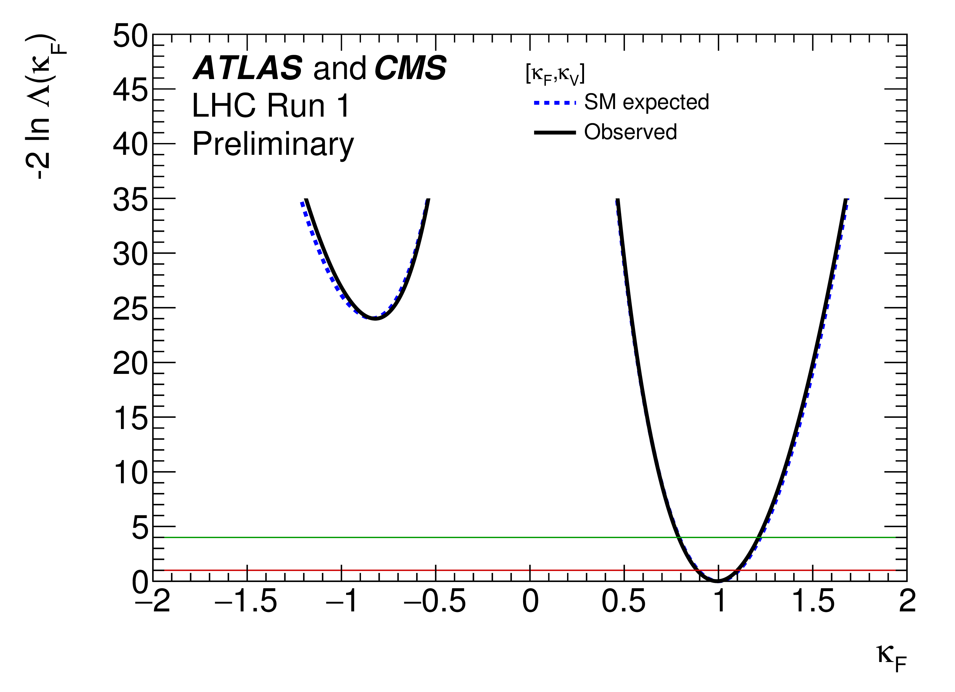
Figure 25-a:
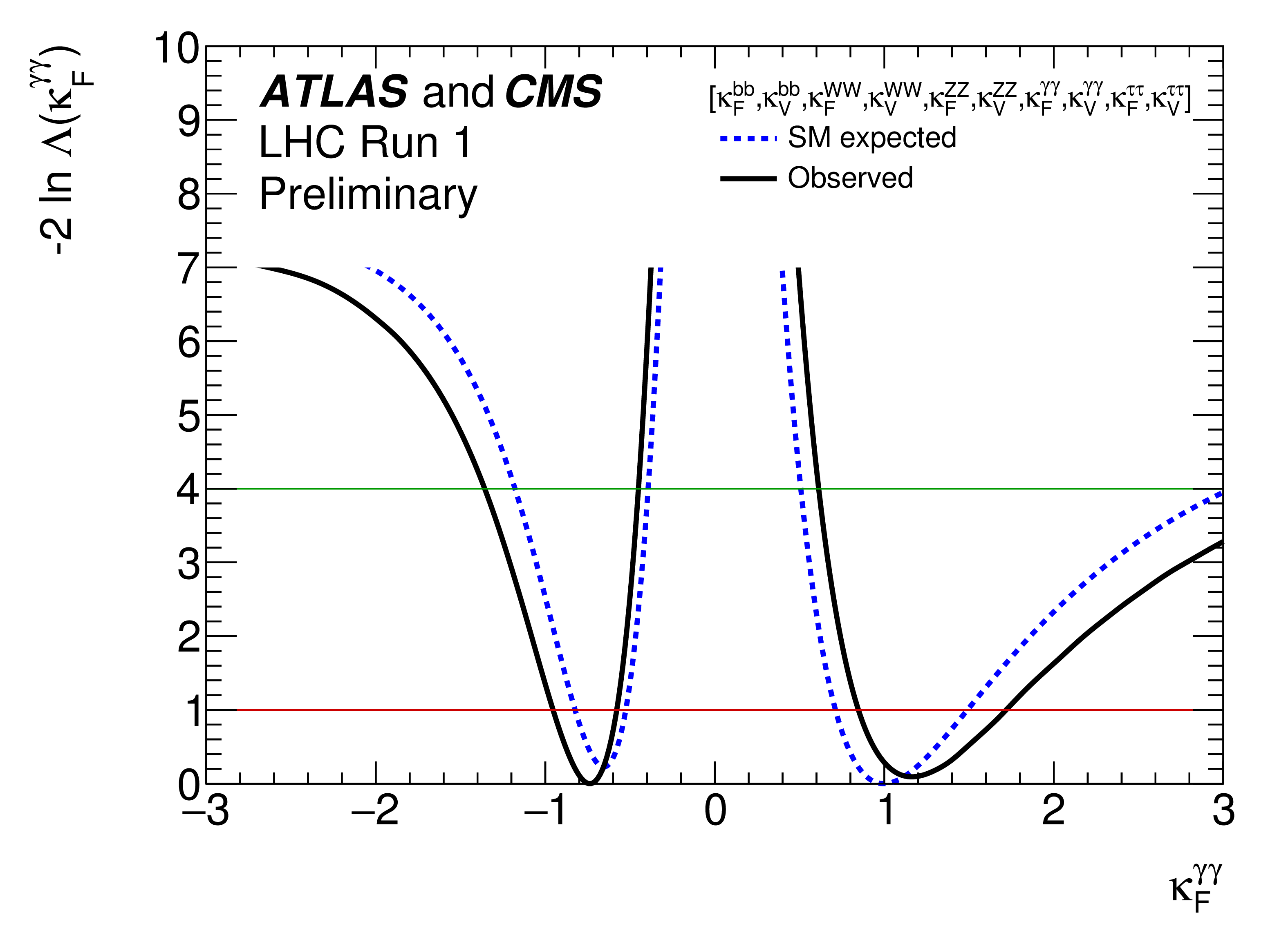
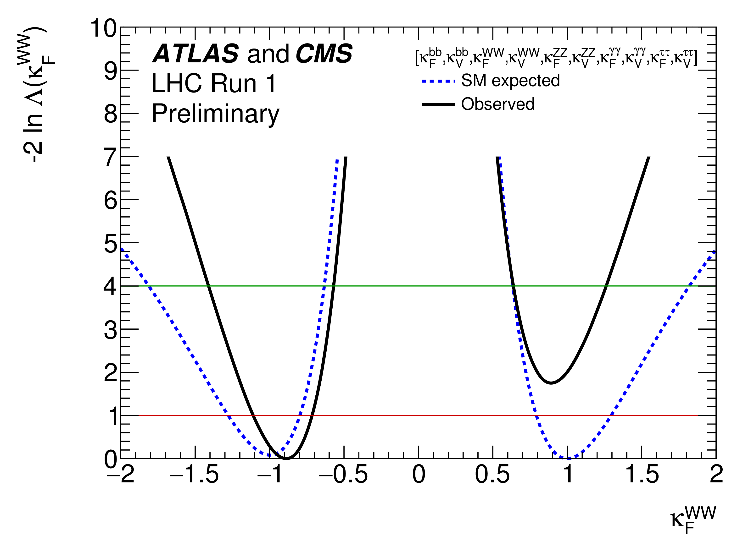
Negative log-likelihood scans for the five $\kappa _F^f$ parameters, corresponding to each individual decay channel, and for the global $\kappa _F$ parameter, corresponding to the combination of all decay channels: (a) $\kappa _{F}^{\gamma \gamma }$, (b) $\kappa _{F}^{ZZ}$, (c) $\kappa _{F}^{WW}$, (d) $\kappa _{F}^{\tau \tau }$, (e) $\kappa _{F}^{bb}$, and (f) $\kappa _F$. |

png ; pdf |
Figure 25-b:
Negative log-likelihood scans for the five $\kappa _F^f$ parameters, corresponding to each individual decay channel, and for the global $\kappa _F$ parameter, corresponding to the combination of all decay channels: (a) $\kappa _{F}^{\gamma \gamma }$, (b) $\kappa _{F}^{ZZ}$, (c) $\kappa _{F}^{WW}$, (d) $\kappa _{F}^{\tau \tau }$, (e) $\kappa _{F}^{bb}$, and (f) $\kappa _F$. |
png ; pdf |
Figure 25-c:
Negative log-likelihood scans for the five $\kappa _F^f$ parameters, corresponding to each individual decay channel, and for the global $\kappa _F$ parameter, corresponding to the combination of all decay channels: (a) $\kappa _{F}^{\gamma \gamma }$, (b) $\kappa _{F}^{ZZ}$, (c) $\kappa _{F}^{WW}$, (d) $\kappa _{F}^{\tau \tau }$, (e) $\kappa _{F}^{bb}$, and (f) $\kappa _F$. |
png ; pdf |
Figure 25-d:
Negative log-likelihood scans for the five $\kappa _F^f$ parameters, corresponding to each individual decay channel, and for the global $\kappa _F$ parameter, corresponding to the combination of all decay channels: (a) $\kappa _{F}^{\gamma \gamma }$, (b) $\kappa _{F}^{ZZ}$, (c) $\kappa _{F}^{WW}$, (d) $\kappa _{F}^{\tau \tau }$, (e) $\kappa _{F}^{bb}$, and (f) $\kappa _F$. |
png ; pdf |
Figure 25-e:
Negative log-likelihood scans for the five $\kappa _F^f$ parameters, corresponding to each individual decay channel, and for the global $\kappa _F$ parameter, corresponding to the combination of all decay channels: (a) $\kappa _{F}^{\gamma \gamma }$, (b) $\kappa _{F}^{ZZ}$, (c) $\kappa _{F}^{WW}$, (d) $\kappa _{F}^{\tau \tau }$, (e) $\kappa _{F}^{bb}$, and (f) $\kappa _F$. |
png ; pdf |
Figure 25-f:
Negative log-likelihood scans for the five $\kappa _F^f$ parameters, corresponding to each individual decay channel, and for the global $\kappa _F$ parameter, corresponding to the combination of all decay channels: (a) $\kappa _{F}^{\gamma \gamma }$, (b) $\kappa _{F}^{ZZ}$, (c) $\kappa _{F}^{WW}$, (d) $\kappa _{F}^{\tau \tau }$, (e) $\kappa _{F}^{bb}$, and (f) $\kappa _F$. |
png ; pdf |
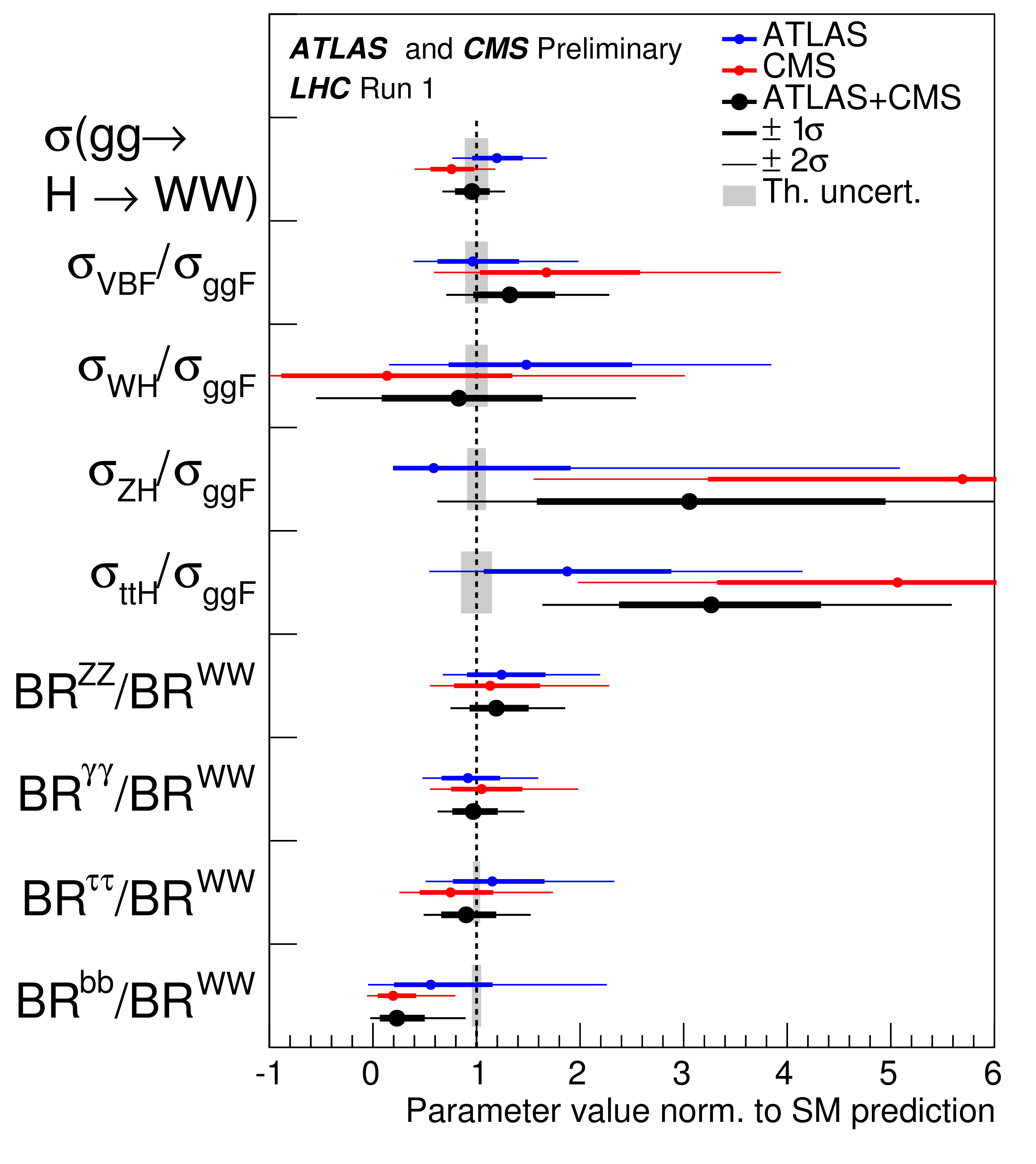
Figure 26:
Best-fit values of the $\sigma (gg\to H\to WW)$ cross section and of ratios of cross sections and branching ratios, as obtained from the generic parameterisation described in Section 4.1 and as tabulated in Table 18 for the combination of ATLAS and CMS measurements. Also shown for completeness are the results for each experiment. The error bars indicate the $1\sigma $ (thick lines) and $2\sigma $ (thin lines) intervals. In this figure, the fit results are normalised to the SM predictions for the various parameters and the shaded bands indicate the theory uncertainties on these predictions. |
png ; pdf |
Figure 27:
Fit results for the combination of ATLAS and CMS in the case of the parameterisation with reduced coupling modifiers $y_{V,i} = \sqrt { {\kappa }_{V,i} \frac {g_{V,i}}{2v} } = \sqrt { {\kappa }_{V,i}}\frac {m_{V,i}}{v}$ for the weak vector bosons, and $y_{F,i} = {\kappa }_{F,i}\frac {g_{F,i}}{\sqrt {2}} = {\kappa }_{F,i}\frac {m_{F,i}}{v}$ for the fermions, as a function of the particle mass. The dashed line indicates the predicted dependence on the particle mass for the SM Higgs boson. The bottom panel shows the ratios of the reduced coupling modifiers to the SM predictions with their total uncertainties as a function of the particle mass. |
png ; pdf |
Figure 28:
Likelihood contours in the ($\mu _{ggF+ttH}^f$, $\mu _{VBF+VH}^f$) plane for the ATLAS+CMS combination, shown for the five decay channels, $ {H\to ZZ}$, $H\to WW$, $ {H\to \gamma \gamma }$, $H\to \tau \tau $, and $H\to bb$. The results are shown as 68% (full) and 95% (dashed) CL contours, together with the best-fit values to the data and the SM expectation. |
| Tables | |
png ; pdf |
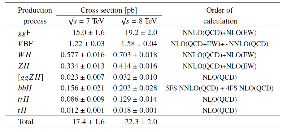
Table 1:
SM predictions for the Higgs boson production cross sections together with their theory uncertainties. The value of the Higgs boson mass is assumed to be $m_H=$ 125.09 GeV and the predictions are obtained by linear interpolation from those at 125.0 and 125.1 GeV from Ref. [26] except for the ${tH}$ cross section, which is obtained from Ref.[62]. The ${ZH}$ cross section includes at NNLO(QCD) both the quark-initiated, i.e. $qq \to ZH$ or $qg \to ZH$, and the $gg\to ZH$ contributions. The contribution from the $ {ggZH}$ production process, indicated in brackets, is given with a theoretical uncertainty assumed to be 30%. The uncertainties on the cross sections are evaluated as the quadratic sum of the uncertainties resulting from variations of QCD scales, parton distribution functions and $\alpha _s$. The uncertainty on the $tH$ cross section is calculated following the procedure of Ref.[28]. The order of the theory calculations for the different production processes is also indicated. |
png ; pdf |
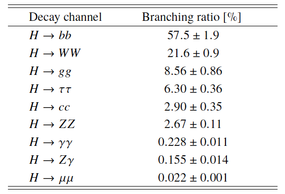
Table 2:
SM predictions for the decay branching ratios of a Higgs boson with a mass of 125.09 GeV, together with their uncertainties. The predictions are obtained from Ref.[26]. Included are decay modes that are either directly studied or important for the combination due to their contributions to the Higgs boson width. |
png ; pdf |
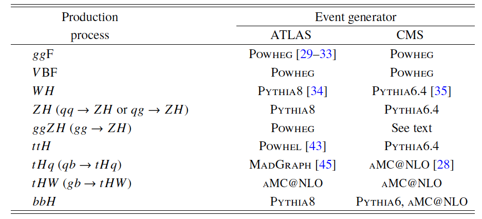
Table 3:
Summary of the event generators used to model the Higgs boson production processes and decay channels at $\sqrt {s}=$ 8 TeV in the ATLAS and CMS experiments. |
png ; pdf |
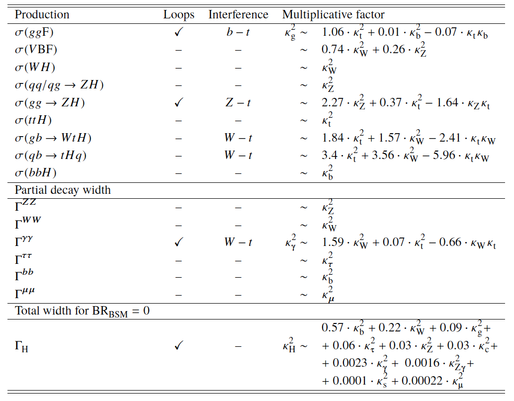
Table 4:
Higgs boson production cross sections $\sigma _{i}$, partial decay widths $\Gamma ^{f}$ and total decay width (in the absence of BSM decays) parameterised as a function of the $ {\kappa }$ coupling modifiers, including higher-order QCD and EW corrections to the inclusive cross sections, as described in Section 2.1. The numerical values are given for $ {\sqrt {s}} =$ 8 TeV and $m_H =$ 125.09 GeV (they are similar for $ {\sqrt {s}} =$ 7 TeV). Contributions which are negligible or not relevant to the analyses presented in this paper are not shown. |
png ; pdf |
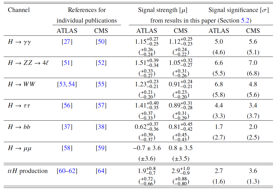
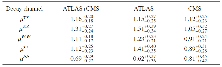
Table 5:
Overview of the decay and production channels analysed in this paper. To show the relative importance of the various channels, the results from the combined analysis presented in this paper for $ {m_{H}} =$ 125.09 GeV (see Tables 10 and 11 in Section 5.2) are shown as observed signal strengths $\mu $ with their uncertainties (the expected uncertainties are shown in parentheses). Also shown are the observed statistical significances (the expected significances are shown in parentheses) except for the $H \to \mu \mu $ channel which has very low sensitivity. For most decay channels, only the most sensitive analyses are quoted as references, e.g. the $ {gg\mathrm {F}}$ and $ {V\mathrm {BF}}$ analyses for the $H\to WW$ decay channel or the $ {VH}$ analysis for the $H\to bb$ decay channel. The results are nevertheless close to those from the individual publications, in which, in addition, slightly different values for the Higgs boson mass were assumed and in which the signal modelling and signal uncertainties were slightly different, as discussed in the text. |
png ; pdf |
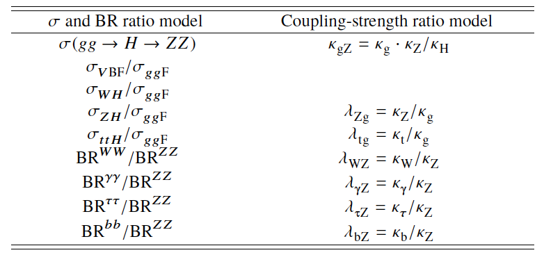
Table 6:
Parameters of interest in the two generic parameterisations described in Sections 4.1 and 4.2. For both parameterisations, the $gg \to H \to ZZ$ channel is chosen as a reference, expressed through the first row in the table. All other measurements are expressed as ratios of cross sections or branching ratios in the first column and of coupling modifiers in the second column. There are more parameters of interest in the case of the first parameterisation, because the ratios of cross sections for the $ {WH}$, $ {ZH}$, and $ {V\mathrm {BF}}$ processes can all be expressed as functions of two parameters $ {\lambda }_{W Z }$ and $ {\lambda }_{Z g }$ in the coupling parameterisation. The slightly different additional assumptions in each parameterisation are discussed in the text. |
png ; pdf |
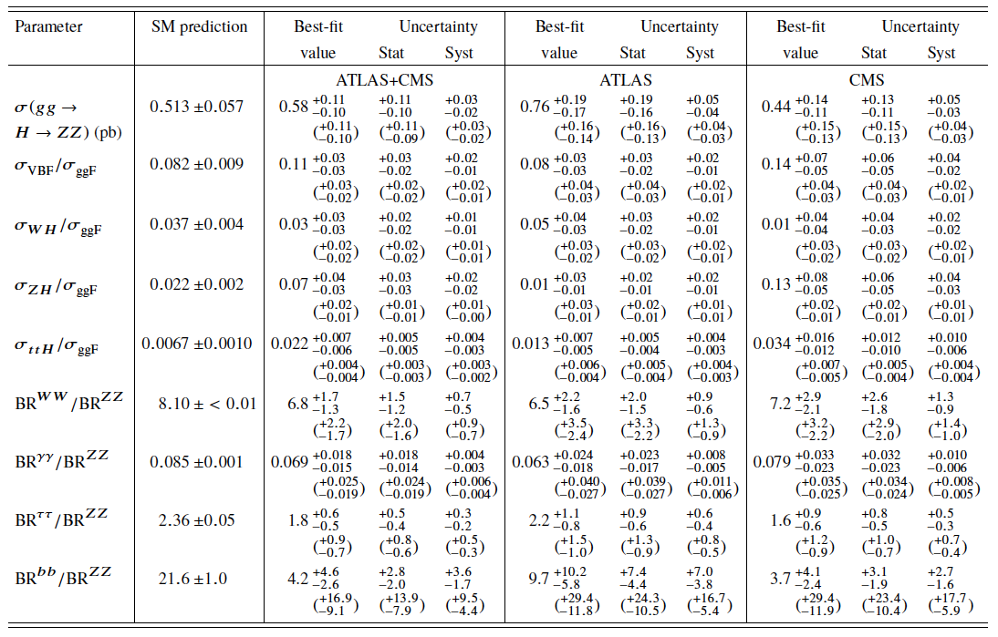
Table 7:
Best-fit values of $\sigma (gg\to H\to ZZ)$, $\sigma _i/\sigma _{\rm ggF}$ and $BR^f/BR^{ZZ}$ from the combined analysis of the $\sqrt {s} =$ 7 and 8 TeV data. The cross-section ratios are given for $\sqrt {s}=$ 8 TeV, assuming the SM values for $\sigma _i(7 \mathrm{TeV} )/\sigma _i(8 \mathrm{TeV} )$. The results are reported for the combination of ATLAS and CMS and also separately for each experiment, together with their total uncertainties and their breakdown into statistical and systematic components. The expected uncertainties on the measurements are also displayed (in parentheses). The SM predictions [26] are also shown with their total uncertainties. |
png ; pdf |
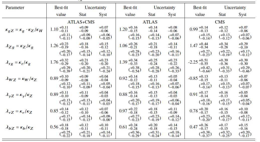
Table 8:
Best-fit values of $ {\kappa }_{g Z }= {\kappa }_{ g }\cdot {\kappa }_{ Z } / {\kappa }_{ H } $ and of the ratios of coupling modifiers, as defined in the most generic model studied in the context of the $ {\kappa }$-framework, from the combined analysis of the $\sqrt {s}=$ 7 and 8 TeV data. The results are shown for the ATLAS+CMS combination and also separately for each experiment, together with their total uncertainties and their breakdown into statistical and systematic components. The total uncertainties on $\lambda _{tg}$ and $\lambda _{WZ}$, for which a negative solution is allowed, are calculated around the overall best-fit value, while the uncertainty breakdown is performed in the positive range. The full ATLAS+CMS 68% CL limits are $\lambda _{WZ} = [-0.97,-0.82] \cup [0.80,0.98]$ and $\lambda _{tg} = [-2.00,-1.55] \cup [1.47,2.08]$. |
png ; pdf |
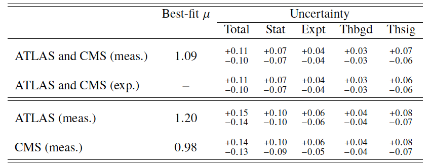
Table 9:
Measured (meas.) global signal strengths $\mu $ together with their total observed and expected (exp.) uncertainties, and with the breakdown of these uncertainties into their four components as defined in Section 3.3. The results are shown for the combination of ATLAS and CMS and separately for each experiment. These results are derived assuming that the Higgs boson production cross sections and branching ratios are the same as in the SM. |
png ; pdf |
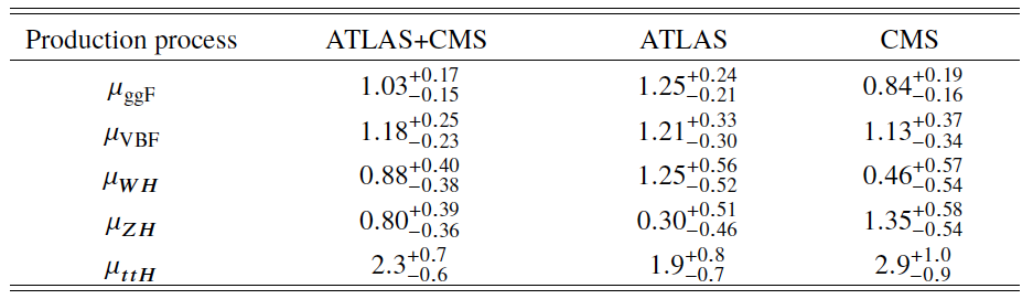
Table 10:
Measured signal strengths $\mu $ and their total uncertainties for different Higgs boson production processes. The results are shown for the combination of ATLAS and CMS and separately for each experiment, for the combined $\sqrt {s}=$ 7 and 8 TeV data. These results are derived assuming that the Higgs boson branching ratios are the same as in the SM. |
png ; pdf |
Table 11:
Measured signal strengths $\mu $ and their total uncertainties for different Higgs boson decay channels. The results are shown for the combination of ATLAS and CMS and separately for each experiment, for the combined $\sqrt {s}=$ 7 and 8 TeV data. These results are derived assuming that the Higgs boson production process cross sections at $\sqrt {s} =$ 7 and 8 TeV are the same as in the SM. |
png ; pdf |
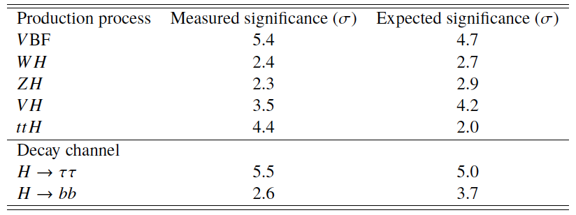
Table 12:
Measured and expected significances for the observation of Higgs boson production processes and decay channels for the combination of ATLAS and CMS. Not included here are the $ {gg\mathrm {F}}$ production process and the $ {H\to ZZ}$, $H\to WW$, and $ {H\to \gamma \gamma }$ decay channels, which have been already clearly observed. All results are obtained constraining the decays to their SM values when considering the production modes, and constraining the production modes to their SM values when studying the decays. |
png ; pdf |
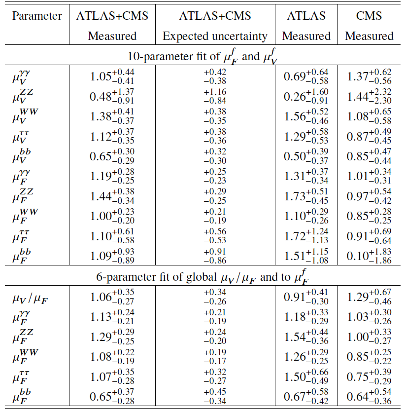
Table 13:
Results of the 10-parameter fit of $\mu _F^f = \mu _{ggF+ttH}^f$ and $\mu _V^f = \mu _{VBF+VH}^f$ for each of the five decay channels, and of the 6-parameter fit of the global ratio $\mu _V/\mu _F = \mu _{VBF+VH}/\mu _{ggF+ttH}$ together with $\mu _F^f$ for each of the five decay channels. The results are shown for the combination of ATLAS and CMS, together with their measured and expected uncertainties, and the measured results are also shown separately for each experiment. |
png ; pdf |
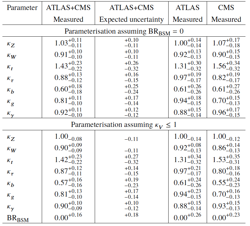
Table 14:
Fit results for the two parameterisations allowing BSM loop couplings, with $ {\kappa }_{V} \le 1$, where $ {\kappa }_{V}$ stands for $ {\kappa }_{Z}$ or $ {\kappa }_{W}$, or without additional BSM contributions to the Higgs boson width, i.e. $ {\mathrm {BR_{BSM}}}=$ 0. The measured results for the combination of ATLAS and CMS are reported together with their measured and expected uncertainties, as well as the measured results for each experiment. The uncertainties are not indicated when the parameters are constrained and hit a boundary, namely $ {\kappa }_{V} =$ 1 or $ {\mathrm {BR_{BSM}}}=$ 0. |
png ; pdf |
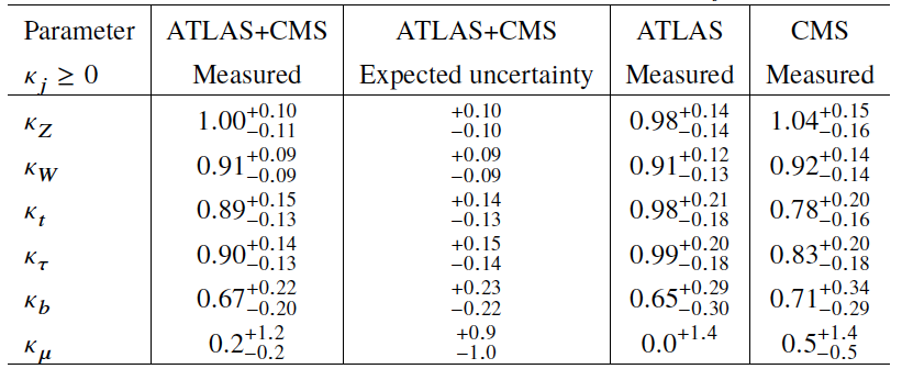
Table 15:
Fit results for the parameterisation assuming the absence of BSM particles in the loops, $ {\mathrm {BR_{BSM}}}=$ 0, and $\kappa _j \ge$ 0. The measured results with their measured and expected uncertainties are reported for the combination of ATLAS and CMS, together with the measured results with their uncertainties for each experiment. The uncertainties are not indicated when the parameters are constrained and hit a boundary, namely $\kappa _j =$ 0. |
png ; pdf |
Table 16:
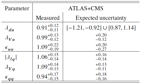
Summary of fit results for the two parameterisations probing the ratios of coupling modifiers for up-type versus down-type fermions and for leptons versus quarks. The measured results are reported for the combination of ATLAS and CMS, together with the measured and expected uncertainties. |
png ; pdf |
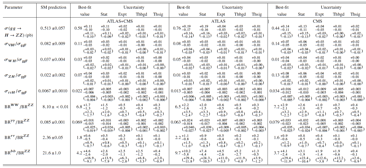
Table 17:
Best-fit values of $\sigma (gg\to H\to ZZ)$, $\sigma _i/\sigma _{\rm ggF}$ and $BR^f/BR^{ZZ}$ from the combined analysis of the $\sqrt {s}=$ 7 and 8 TeV data. The cross-section ratios are given for $\sqrt {s}= $ 8 TeV, assuming the SM values for $\sigma _i(7 \mathrm{TeV} )/\sigma _i(8 \mathrm{TeV} )$. The results are shown for the ATLAS+CMS combination and also separately for each experiment, together with their total uncertainties and their breakdown into the four components described in the text. The expected total uncertainties on the measurements are also shown (in parentheses). The SM predictions [26] are also shown with their total uncertainties. |
png ; pdf |
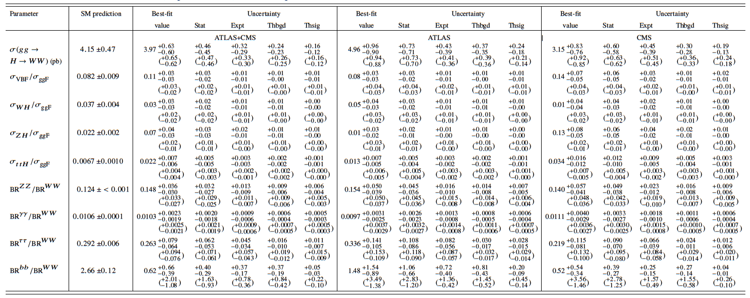
Table 18:
Best-fit values of $\sigma (gg\to H\to WW)$, $\sigma _i/\sigma _{\rm ggF}$ and $BR^f/BR^{WW}$ from the combined analysis of the $\sqrt {s}=7$ and 8 TeV data. The cross-section ratios are given for $\sqrt {s}=8$ TeV, assuming the SM values for $\sigma _i(7 \mathrm{TeV} )/\sigma _i(8 \mathrm{TeV} )$. The results are shown for the ATLAS+CMS combination and also separately for each experiment, together with their total uncertainties and their breakdown into the four components described in the text. The expected total uncertainties on the measurements are also shown (in parentheses). The SM predictions [26] are also shown with their total uncertainties. |

png ; pdf |
Table 19:
Best-fit values of $ {\kappa }_{g Z }= {\kappa }_{g }\cdot {\kappa }_{Z } / {\kappa }_{H } $ and of the ratios of coupling modifiers, as defined in the most generic model described in the context of the $ {\kappa }$ framework, from the combined analysis of the $\sqrt {s}=$ 7 and 8 TeV data. The results are shown for the ATLAS+CMS combination and also separately for each experiment, together with their total uncertainties and their breakdown into the four components described in the text. The total uncertainties on $\lambda _{WZ}$ and $\lambda _{tg}$, for which a negative solution is allowed, are calculated around the overall best-fit value, while the uncertainty breakdown is performed in the positive range. The full ATLAS+CMS 68% CL limits are $\lambda _{tg} = [-2.00,-1.55] \cup [1.47,2.08]$ and $\lambda _{WZ} = [-0.97,-0.82] \cup [0.80,0.98]$. |
png ; pdf |
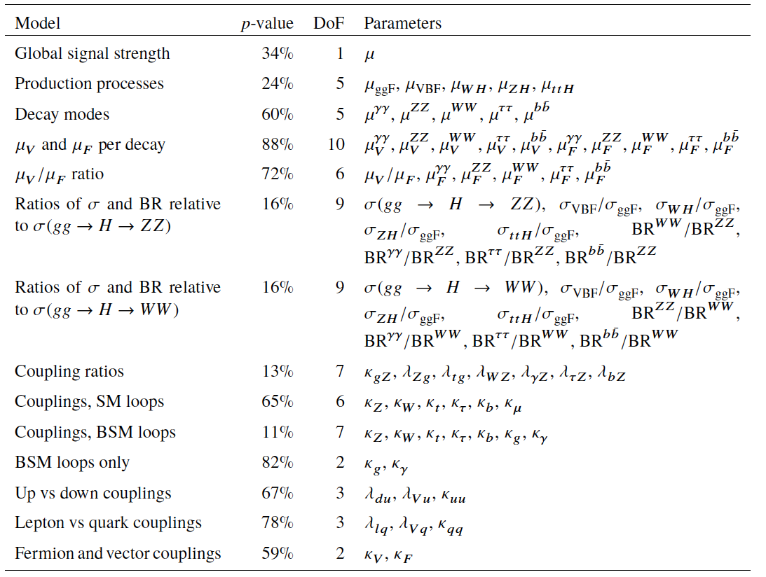
Table 20:
Compatibility with the SM prediction of fit results as a whole under the asymptotic approximation. For each model, the unconditional best-fit is compared with the conditional fit where all parameters are set to their SM values. The conversion from $-2\ln\Lambda $ to the quoted $p$-value is performed assuming a two-sided distribution with the specified number of degrees of freedom (DoF). Note that the quoted $p$-values are partially correlated between the different models. |
| Summary |
| Combined ATLAS and CMS measurements of the Higgs boson production and decay rates have been performed and constraints on its couplings to vector bosons and fermions have been derived. The combination is based on the analysis of five production processes, $gg$F, $V$BF, $WH$, $ZH$ and $ttH$, and of six decay channels, $H \to ZZ$, $WW$, $\gamma \gamma$, $\tau \tau$, $bb$ and $\mu \mu$. All results are reported assuming a value of 125.09 GeV for the Higgs boson mass, the result of the combined Higgs boson mass measurement by the two experiments. The analysis uses the LHC proton-proton collision datasets recorded by the ATLAS and CMS detectors in 2011 and 2012, corresponding to integrated luminosities per experiment of approximately 5 fb$^{-1}$ at $ \sqrt{s} =$ 7 TeV and 20 fb$^{-1}$ at $\sqrt{s} =$ 8 TeV. The Higgs boson production and decay rates of the two experiments are combined within the context of two generic parameterisations: one based on ratios of cross sections and branching ratios and the other based on ratios of coupling modifiers, introduced within the context of a leading-order Higgs boson coupling framework. The combined signal yield relative to the Standard Model expectation is measured to be 1.09 $\pm$ 0.11 and the combination of the two experiments leads to observed significances of the $V$BF production process and of the $H \to \tau\tau$ decay at the level of 5.4$\sigma$ and 5.5$\sigma$, respectively. Several interpretations of the results with more model-dependent parameterisations, derived from the generic ones, are also given. The data are consistent with the StandardModel predictions for all parameterisations considered. |
|
|
Compact Muon Solenoid LHC, CERN |
|

|

|

|

|

|