

Compact Muon Solenoid
LHC, CERN
| CMS-PAS-EXO-15-007 | ||
| Search for black holes at $ \sqrt{s} = $ 13 TeV | ||
| CMS Collaboration | ||
| December 2015 | ||
| Abstract: A search for black holes using a data sample corresponding to an integrated luminosity of 2.2 fb$^{-1}$ collected with the CMS experiment at the LHC in pp collisions at a center-of-mass energy of 13 TeV in 2015 is presented. No excess characteristic of a black hole production or other new physics signals resulting in energetic multiparticle final states was observed. Standard model background, dominated by QCD multijet production, was determined exclusively from control regions in data, without any reliance on simulation. Model-independent limits on the cross section of a new physics signal in these final states are set and further interpreted in terms of limits on black hole production. In the context of models with large extra dimensions, semiclassical black holes with masses below $\sim$ 8.7 TeV and quantum black holes with masses below $\sim$ 8 TeV are excluded by this search, thus significantly extending limits set in the LHC Run 1. | ||
|
Links:
CDS record (PDF) ;
CADI line (restricted) ;
These preliminary results are superseded in this paper, PLB 774 (2017) 279. The superseded preliminary plots can be found here. |
||
| Figures | |
png ; pdf ; |
Figure 1:
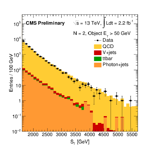
Contributions of the main QCD multijet background, as well as V+jets (where V = Z, W), $ {\gamma }$ + jets, and $ \mathrm{ t \bar{t} } $ + jets backgrounds to the $ {S_{\mathrm {T}}} $ distribution for multiplicity $N=$ 2. |
png ; pdf ; |
Figure 2-a:
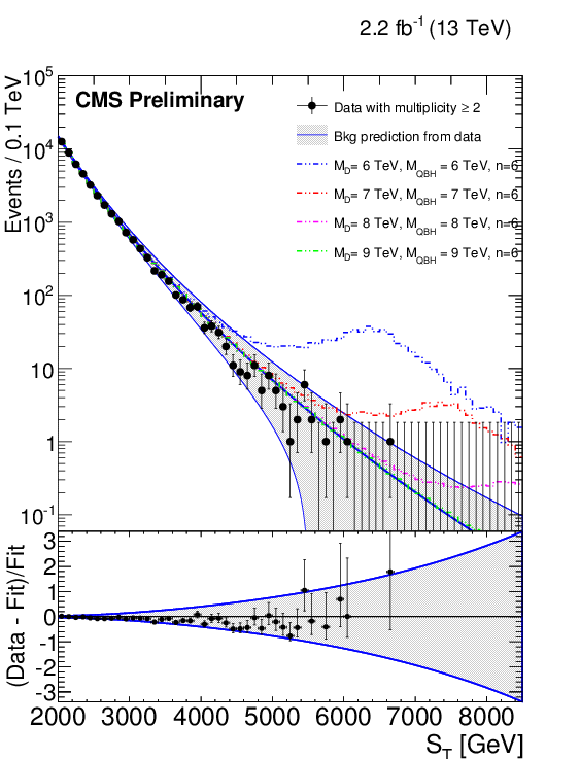
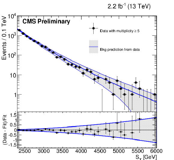
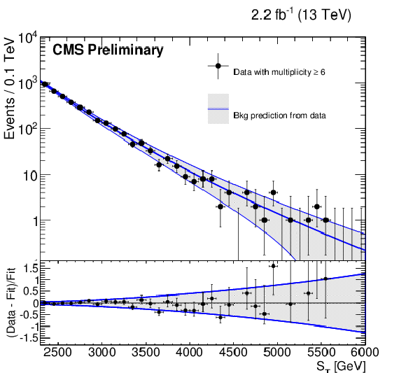
The distributions of the total transverse energy, $ {S_{\mathrm {T}}} $ for inclusive multiplicities of objects (photons, muons, photons or jets) $ N \geq $ 2, 3, 4, 5. Observed data are shown by points with error bars, the solid blue lines along with the grey shaded band show the main background estimation (central blue line), along with the uncertainty band (outer blue lines). The deviation of the fit from the data is shown in the lower panes. The top two plots also show several quantum black hole signal points. |
png ; pdf ; |
Figure 2-b:
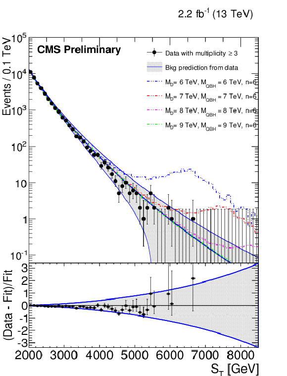
The distributions of the total transverse energy, $ {S_{\mathrm {T}}} $ for inclusive multiplicities of objects (photons, muons, photons or jets) $ N \geq $ 2, 3, 4, 5. Observed data are shown by points with error bars, the solid blue lines along with the grey shaded band show the main background estimation (central blue line), along with the uncertainty band (outer blue lines). The deviation of the fit from the data is shown in the lower panes. The top two plots also show several quantum black hole signal points. |
png ; pdf ; |
Figure 2-c:
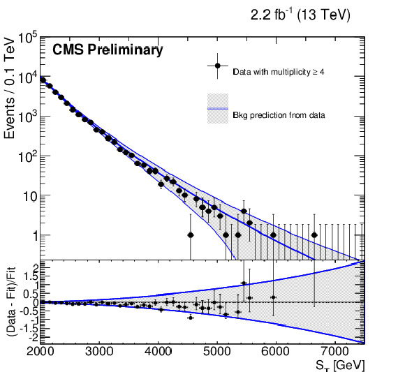
The distributions of the total transverse energy, $ {S_{\mathrm {T}}} $ for inclusive multiplicities of objects (photons, muons, photons or jets) $ N \geq $ 2, 3, 4, 5. Observed data are shown by points with error bars, the solid blue lines along with the grey shaded band show the main background estimation (central blue line), along with the uncertainty band (outer blue lines). The deviation of the fit from the data is shown in the lower panes. The top two plots also show several quantum black hole signal points. |
png ; pdf ; |
Figure 2-d:
The distributions of the total transverse energy, $ {S_{\mathrm {T}}} $ for inclusive multiplicities of objects (photons, muons, photons or jets) $ N \geq $ 2, 3, 4, 5. Observed data are shown by points with error bars, the solid blue lines along with the grey shaded band show the main background estimation (central blue line), along with the uncertainty band (outer blue lines). The deviation of the fit from the data is shown in the lower panes. The top two plots also show several quantum black hole signal points. |
png ; pdf ; |
Figure 3-a:
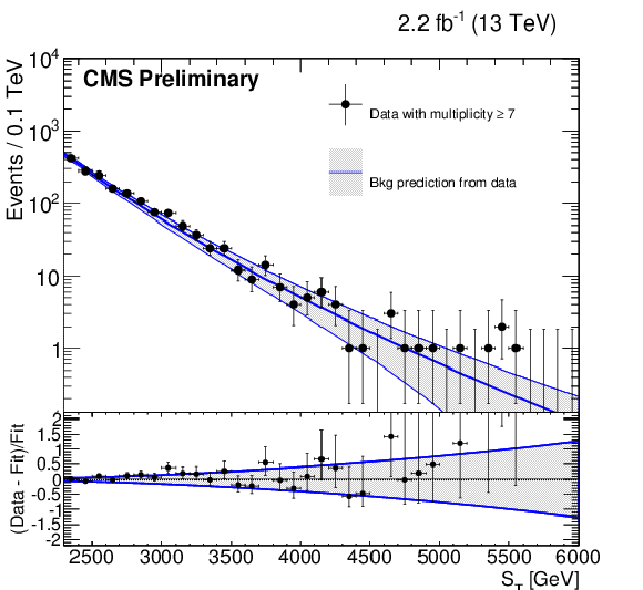
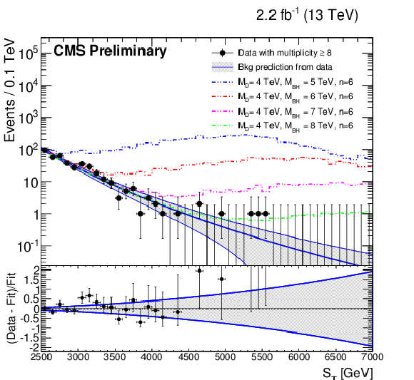
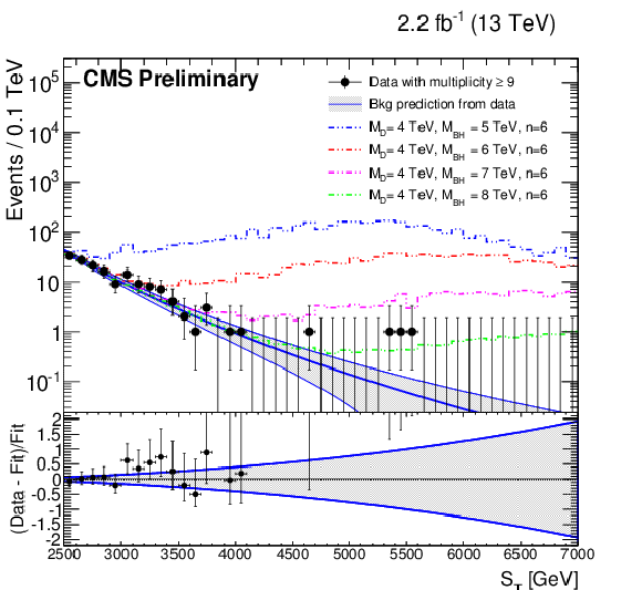
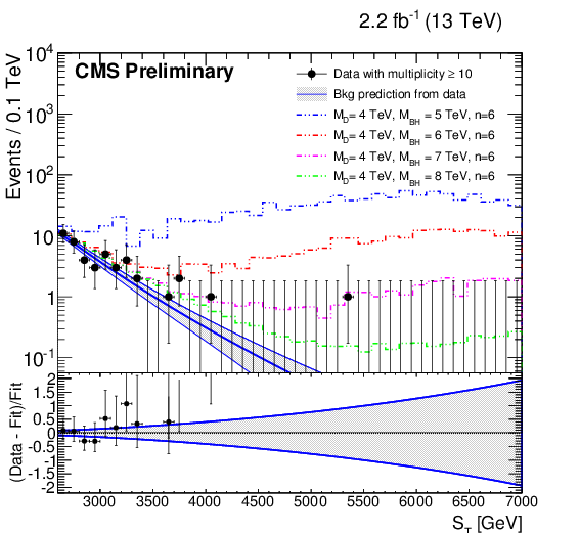
The distributions of the total transverse energy, $ {S_{\mathrm {T}}} $ for inclusive multiplicities of objects (photons, muons, photons or jets) $ N \geq $ 6, 7, 8, 9, 10. Observed data are shown by points with error bars, the solid blue lines along with the grey shaded band show the main background estimation (central blue line), along with the uncertainty band (outer blue lines). The deviation of the fit from the data is shown in the lower panes. The (c,d,f) plots also show several semiclassical black hole signal points. |
png ; pdf ; |
Figure 3-b:
The distributions of the total transverse energy, $ {S_{\mathrm {T}}} $ for inclusive multiplicities of objects (photons, muons, photons or jets) $ N \geq $ 6, 7, 8, 9, 10. Observed data are shown by points with error bars, the solid blue lines along with the grey shaded band show the main background estimation (central blue line), along with the uncertainty band (outer blue lines). The deviation of the fit from the data is shown in the lower panes. The (c,d,f) plots also show several semiclassical black hole signal points. |
png ; pdf ; |
Figure 3-c:
The distributions of the total transverse energy, $ {S_{\mathrm {T}}} $ for inclusive multiplicities of objects (photons, muons, photons or jets) $ N \geq $ 6, 7, 8, 9, 10. Observed data are shown by points with error bars, the solid blue lines along with the grey shaded band show the main background estimation (central blue line), along with the uncertainty band (outer blue lines). The deviation of the fit from the data is shown in the lower panes. The (c,d,f) plots also show several semiclassical black hole signal points. |
png ; pdf ; |
Figure 3-d:
The distributions of the total transverse energy, $ {S_{\mathrm {T}}} $ for inclusive multiplicities of objects (photons, muons, photons or jets) $ N \geq $ 6, 7, 8, 9, 10. Observed data are shown by points with error bars, the solid blue lines along with the grey shaded band show the main background estimation (central blue line), along with the uncertainty band (outer blue lines). The deviation of the fit from the data is shown in the lower panes. The (c,d,f) plots also show several semiclassical black hole signal points. |
png ; pdf ; |
Figure 3-e:
The distributions of the total transverse energy, $ {S_{\mathrm {T}}} $ for inclusive multiplicities of objects (photons, muons, photons or jets) $ N \geq $ 6, 7, 8, 9, 10. Observed data are shown by points with error bars, the solid blue lines along with the grey shaded band show the main background estimation (central blue line), along with the uncertainty band (outer blue lines). The deviation of the fit from the data is shown in the lower panes. The (c,d,f) plots also show several semiclassical black hole signal points. |
png ; pdf ; |
Figure 4-a:
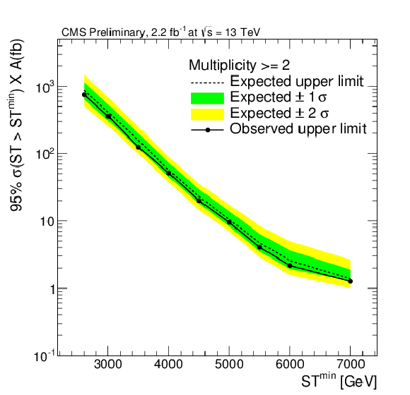
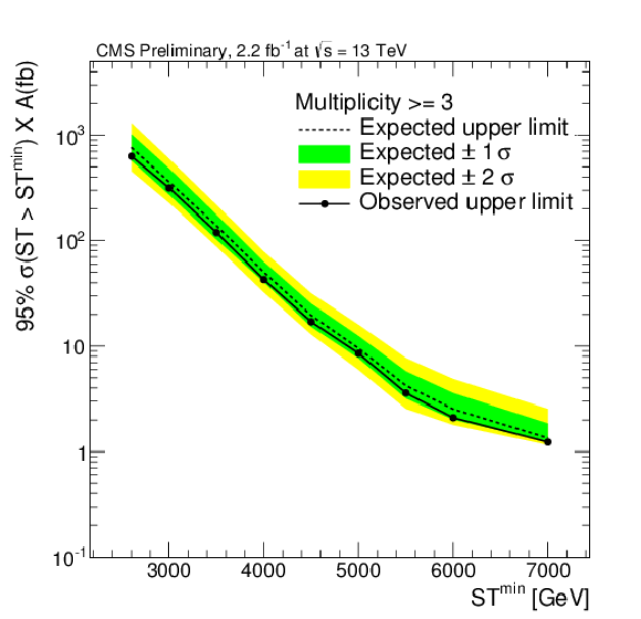
Model-independent upper limits on the cross section times acceptance for four sets of inclusive multiplicity thresholds: a) $ N \ge $ 2, b) $ N \geq $ 3, c) $ N \geq $ 4, and d) $ N \geq $ 5. Observed (expected) limits are shown as solid (dotted) lines. |
png ; pdf ; |
Figure 4-b:
Model-independent upper limits on the cross section times acceptance for four sets of inclusive multiplicity thresholds: a) $ N \ge $ 2, b) $ N \geq $ 3, c) $ N \geq $ 4, and d) $ N \geq $ 5. Observed (expected) limits are shown as solid (dotted) lines. |
png ; pdf ; |
Figure 4-c:
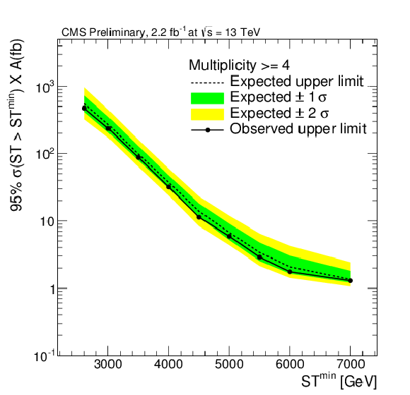
Model-independent upper limits on the cross section times acceptance for four sets of inclusive multiplicity thresholds: a) $ N \ge $ 2, b) $ N \geq $ 3, c) $ N \geq $ 4, and d) $ N \geq $ 5. Observed (expected) limits are shown as solid (dotted) lines. |
png ; pdf ; |
Figure 4-d:
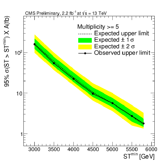
Model-independent upper limits on the cross section times acceptance for four sets of inclusive multiplicity thresholds: a) $ N \ge $ 2, b) $ N \geq $ 3, c) $ N \geq $ 4, and d) $ N \geq $ 5. Observed (expected) limits are shown as solid (dotted) lines. |
png ; pdf ; |
Figure 5-a:
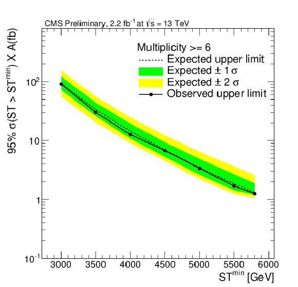
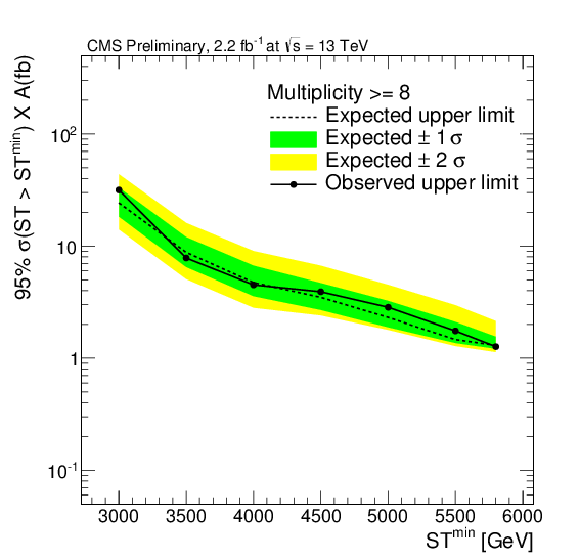
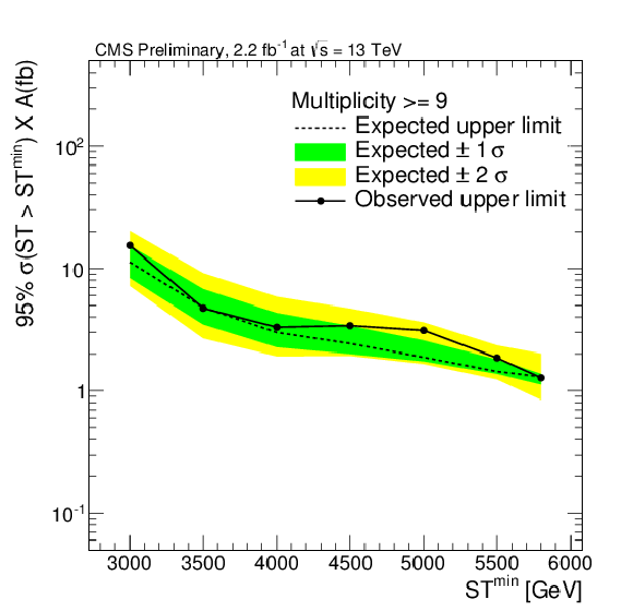
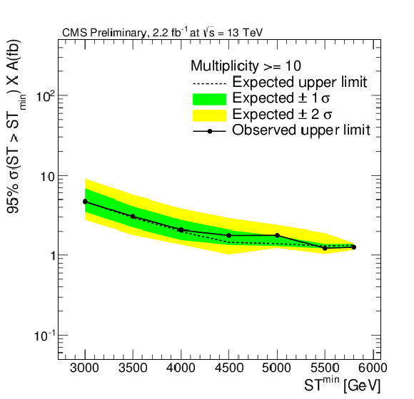
Model-independent upper limits on the cross section times acceptance for four sets of inclusive multiplicity thresholds: a) $ N \ge $ 6, b) $ N \geq $ 7, c) $ N \geq $ 8, d) $ N \geq $ 9, and e) $ N \geq $ 10. Observed (expected) limits are shown as a solid (dotted) line. |
png ; pdf ; |
Figure 5-b:
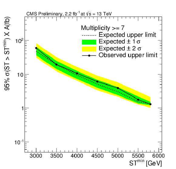
Model-independent upper limits on the cross section times acceptance for four sets of inclusive multiplicity thresholds: a) $ N \ge $ 6, b) $ N \geq $ 7, c) $ N \geq $ 8, d) $ N \geq $ 9, and e) $ N \geq $ 10. Observed (expected) limits are shown as a solid (dotted) line. |
png ; pdf ; |
Figure 5-c:
Model-independent upper limits on the cross section times acceptance for four sets of inclusive multiplicity thresholds: a) $ N \ge $ 6, b) $ N \geq $ 7, c) $ N \geq $ 8, d) $ N \geq $ 9, and e) $ N \geq $ 10. Observed (expected) limits are shown as a solid (dotted) line. |
png ; pdf ; |
Figure 5-d:
Model-independent upper limits on the cross section times acceptance for four sets of inclusive multiplicity thresholds: a) $ N \ge $ 6, b) $ N \geq $ 7, c) $ N \geq $ 8, d) $ N \geq $ 9, and e) $ N \geq $ 10. Observed (expected) limits are shown as a solid (dotted) line. |
png ; pdf ; |
Figure 5-e:
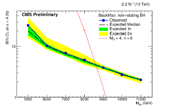
Model-independent upper limits on the cross section times acceptance for four sets of inclusive multiplicity thresholds: a) $ N \ge $ 6, b) $ N \geq $ 7, c) $ N \geq $ 8, d) $ N \geq $ 9, and e) $ N \geq $ 10. Observed (expected) limits are shown as a solid (dotted) line. |
png ; pdf ; |
Figure 6-a:
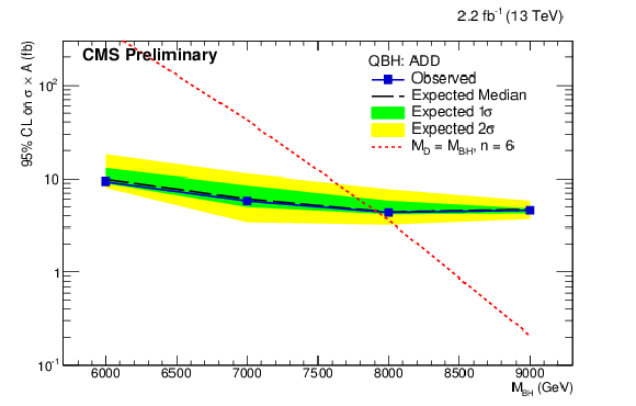
(a) Observed and expected upper 95% CL cross section times acceptance limits overlaid with the predicted values for a semiclassical BH with $M_D =$ 4 TeV, $ n= $ 6, and varying $ {M_{\mathrm {BH}}^\text {min}} $, at the multiplicity and $ {S_{\mathrm {T}}^\text {min}} $ values maximizing the $Z_{Bi}$ test statistic. Depending on the signal point, optimal sensitivity is achieved for $ N \ge $ 9 or 10. (b) Same for a quantum BH model with $ {M_{\mathrm {BH}}^\text {min}} = M_D$; in this case the limits come from the $ N \ge $ 3 spectrum, which provides optimal sensitivity. |
png ; pdf ; |
Figure 6-b:
(a) Observed and expected upper 95% CL cross section times acceptance limits overlaid with the predicted values for a semiclassical BH with $M_D =$ 4 TeV, $ n= $ 6, and varying $ {M_{\mathrm {BH}}^\text {min}} $, at the multiplicity and $ {S_{\mathrm {T}}^\text {min}} $ values maximizing the $Z_{Bi}$ test statistic. Depending on the signal point, optimal sensitivity is achieved for $ N \ge $ 9 or 10. (b) Same for a quantum BH model with $ {M_{\mathrm {BH}}^\text {min}} = M_D$; in this case the limits come from the $ N \ge $ 3 spectrum, which provides optimal sensitivity. |
png ; pdf ; |
Figure 7:
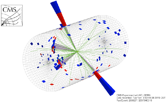
Event display for a quantum black hole candidate collected in Run 260627, Event 2097040310. This event has 4 jets, $S_T$ of 6.67 TeV, $ {E_{\mathrm {T}}^{\text {miss}}} $ of 110 GeV, and the multiplicity $ N = $ 4. |
png ; pdf ; |
Figure 8:
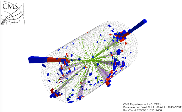
Event display for a black hole candidate collected in Run 259685, Event 155512460. This event has 9 jets, $S_T$ of 5.56 TeV, $ {E_{\mathrm {T}}^{\text {miss}}} $ of 8.4 GeV, and the multiplicity $ N = $ 9. |
png ; pdf ; |
Figure 9:
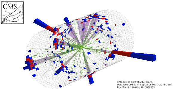
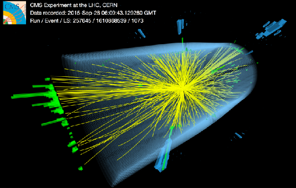
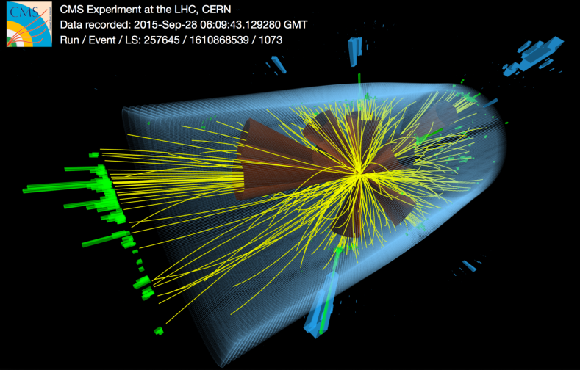
Event display for a black hole candidate collected in Run 257645, Event 1610868539. This event has 12 jets, $S_T$ of 5.48 TeV, $ {E_{\mathrm {T}}^{\text {miss}}} $ of 120 GeV, and the multiplicity $ N = $ 12. |
| Auxiliary Figures | |
png ; pdf ; |
Auxiliary Figure 1-a:
Artistic renderings of an event display for a black hole candidate collected in Run 257645, Event 1610868539. This event has 12 jets, $S_T$ of 5.48 TeV, $E_{\mathrm{T}}^{\text{miss}}$ of 120 GeV, and the multiplicity $N = $ 12. |
png ; pdf ; |
Auxiliary Figure 1-b:
Artistic renderings of an event display for a black hole candidate collected in Run 257645, Event 1610868539. This event has 12 jets, $S_T$ of 5.48 TeV, $E_{\mathrm{T}}^{\text{miss}}$ of 120 GeV, and the multiplicity $N = $ 12. |

|
Compact Muon Solenoid LHC, CERN |

|

|

|

|

|

|