CMS-PAS-BPH-15-002

CMS-PAS-BPH-15-002
Measurement of the $\Lambda_{b}$ polarization and the angular parameters of the decay $\Lambda_{b}\to J/\psi(\mu^{+}\mu^{-}) \Lambda^{0}(p\pi^{-})$
CMS Collaboration
August 2016

Abstract: We present a measurement of the $\Lambda_{b}$ polarization based on an angular analysis of the decay $\Lambda_{b}\to J/\psi(\mu^{+}\mu^{-}) \Lambda^{0}(p\pi^{-})$, using data from pp collisions at $\sqrt{s} =$ 7 TeV and 8 TeV collected with the CMS detector. A transverse $\Lambda_{b}$ polarization of 0.00 $\pm$ 0.06 (stat) $\pm$ 0.02 (syst) is measured.
Links: CDS record (PDF) ; CADI line (restricted) ; These preliminary results are superseded in this paper, PRD 97 (2018) 072010. The superseded preliminary plots can be found here.

Figures & Tables	Summary	References	CMS Publications

Figures
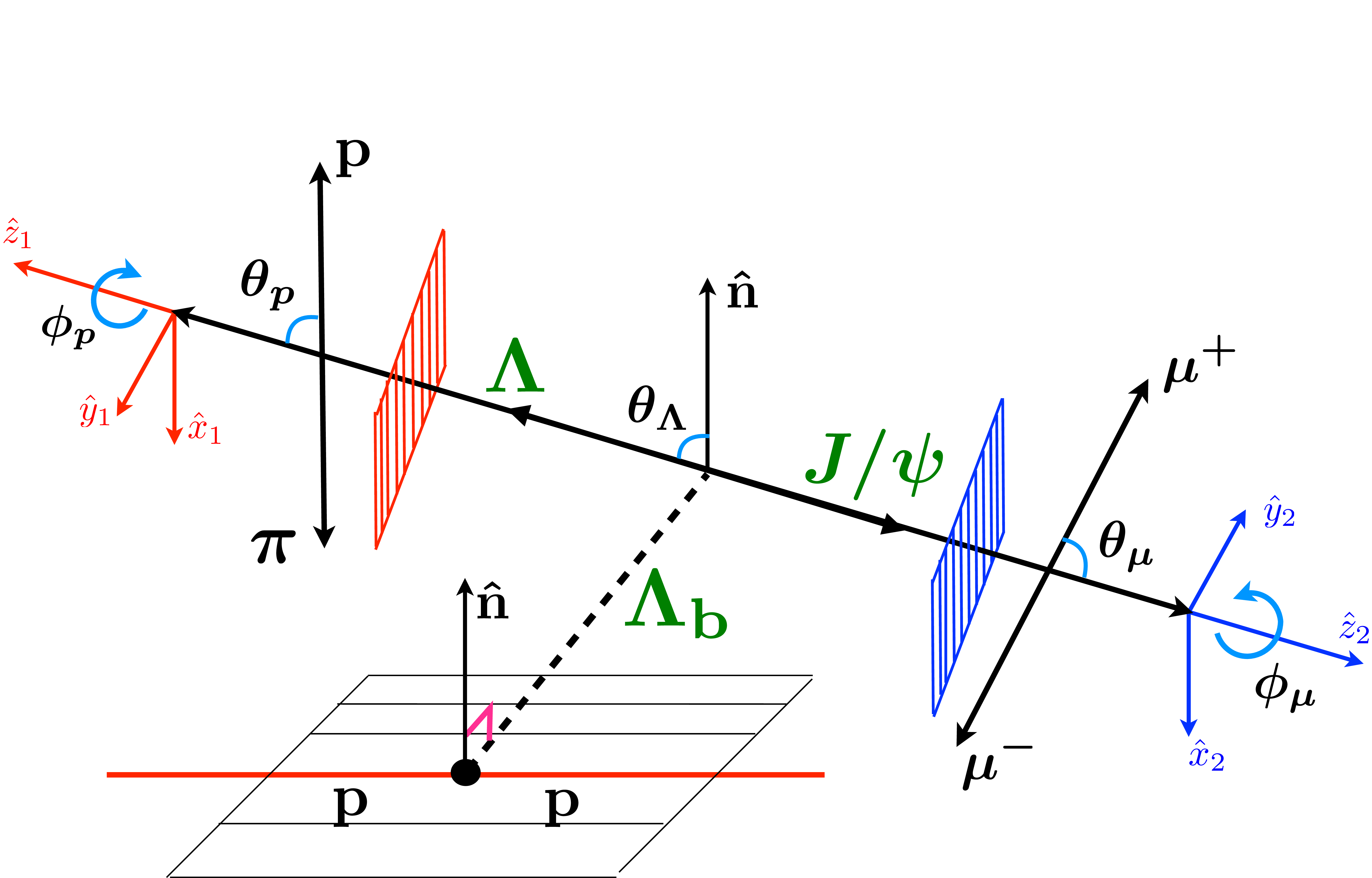
png pdf	Figure 1: Definition of the angles used to describe the $\Lambda _{b} \rightarrow J/\psi (\rightarrow \mu ^{+}\mu ^{-})\Lambda ^{0}(\rightarrow p\pi ^{-})$ decay.
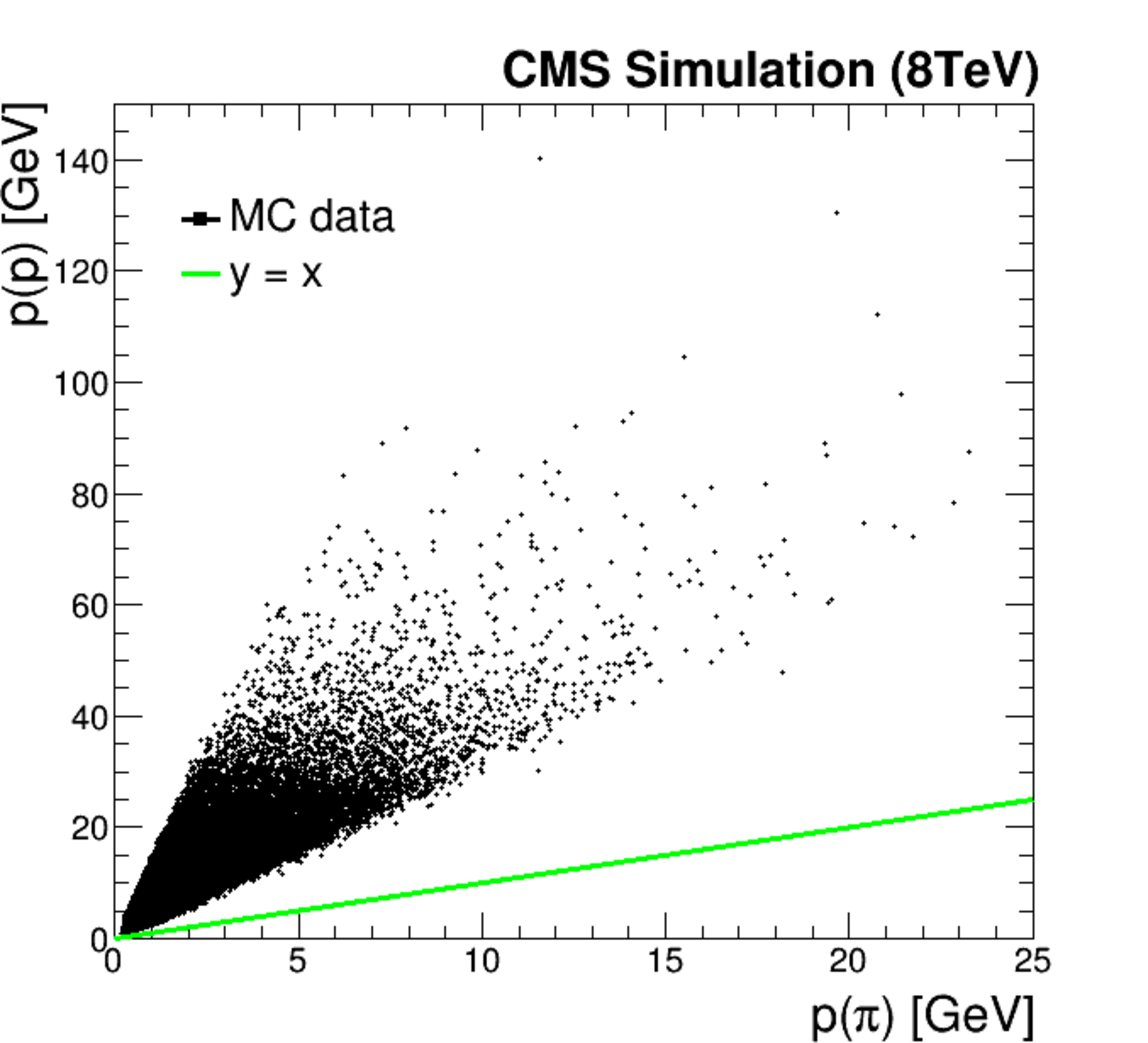
png pdf	Figure 2: Distribution of the $p$ vs $\pi $ momentum obtained from the simulation of $\Lambda _{b}\to J/\psi \Lambda (p \pi ^{-})$ (and complex conjugate) decays. Events lie always above the green line, ie., the $p^{+}$ ($p^{-}$) momentum is always greater than $\pi ^{-}$ ($\pi ^{+}$) momentum.
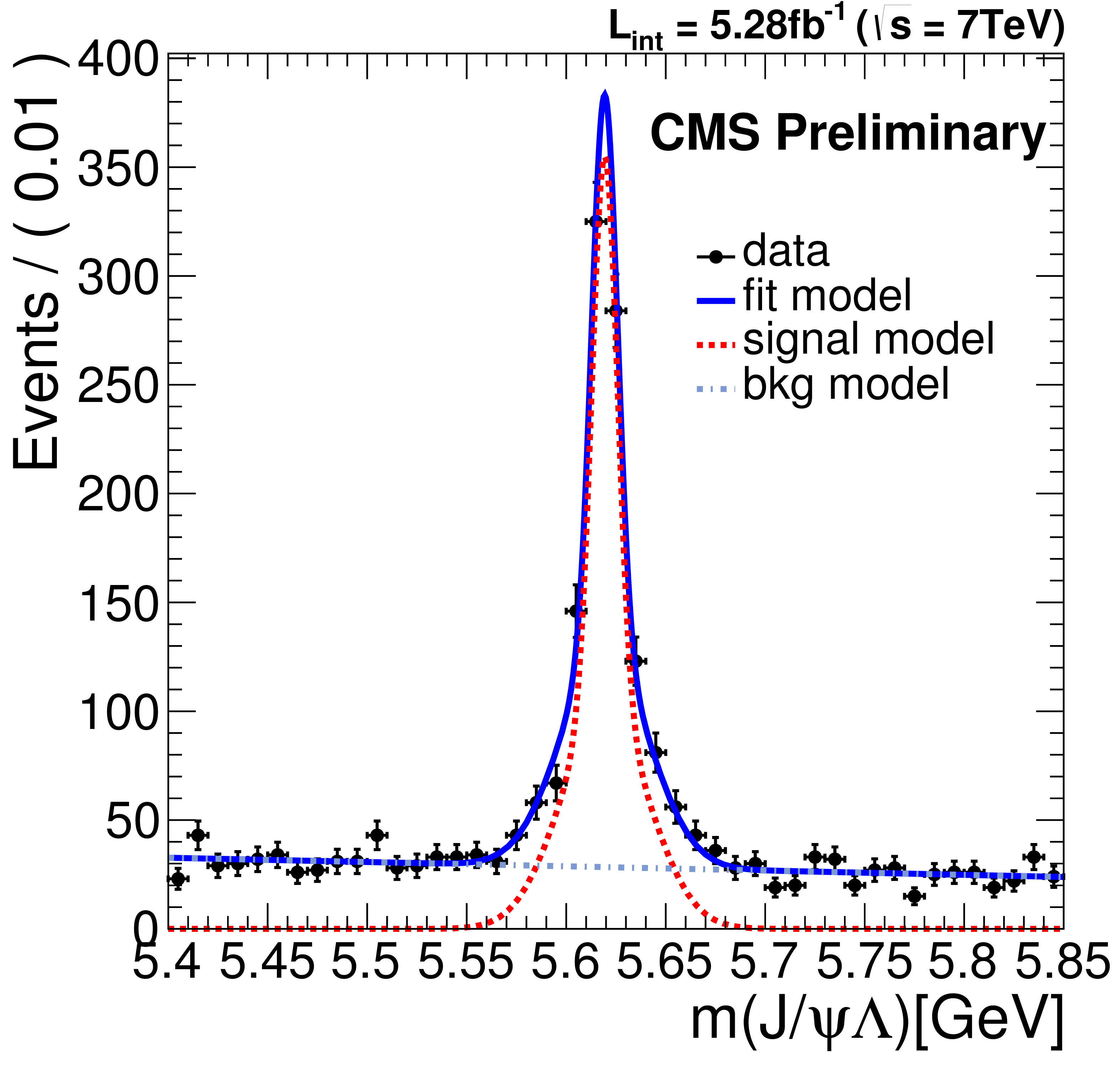
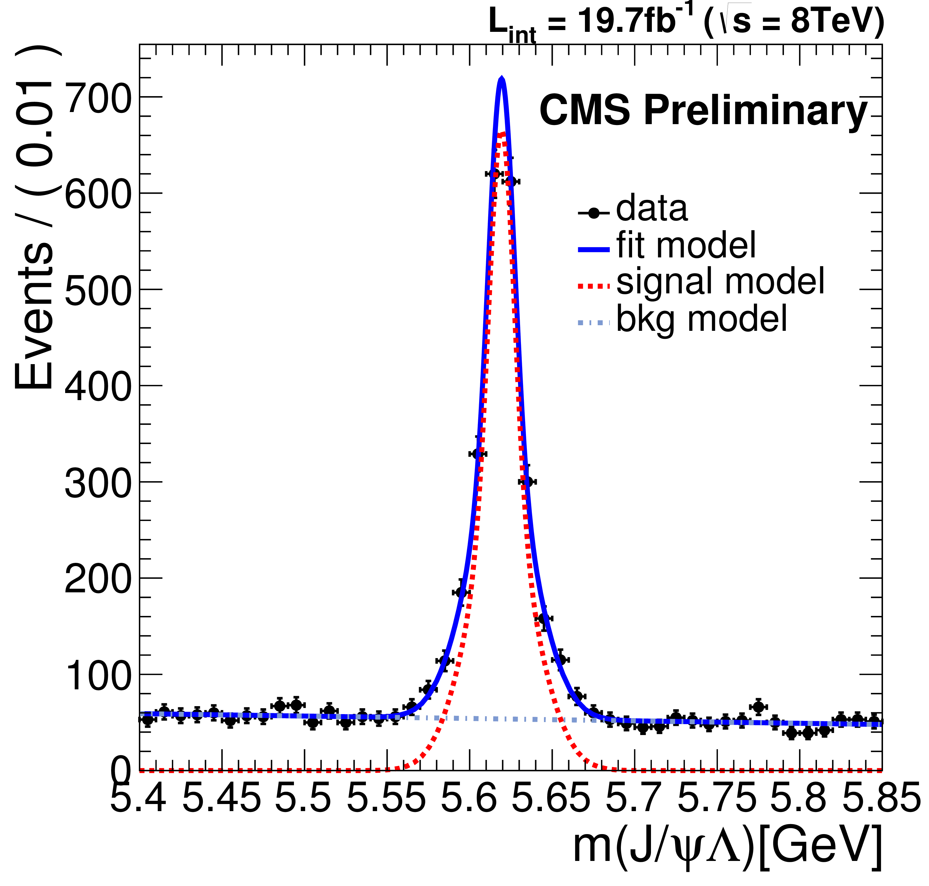
png pdf	Figure 3-a: Invariant mass distribution of $\Lambda_b$ (a and c) and $\overline{\Lambda}_b$ (b and d) candidates in (a-b) 2011 and (c-d) 2012 samples. The solid blue line represents the fit result. The signal (background) projection is shown with a dashed (dot-dashed) red (blue) line.
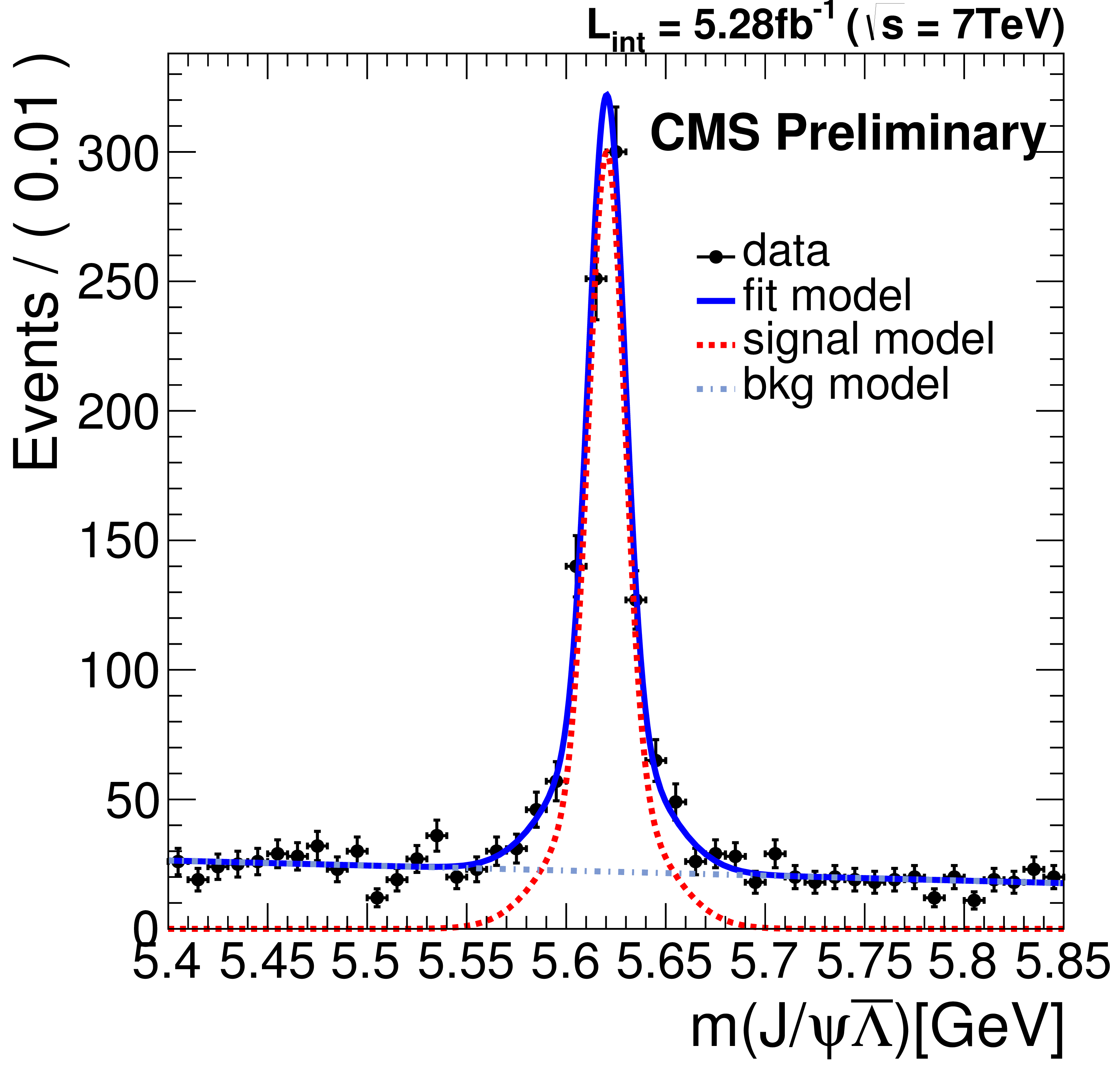
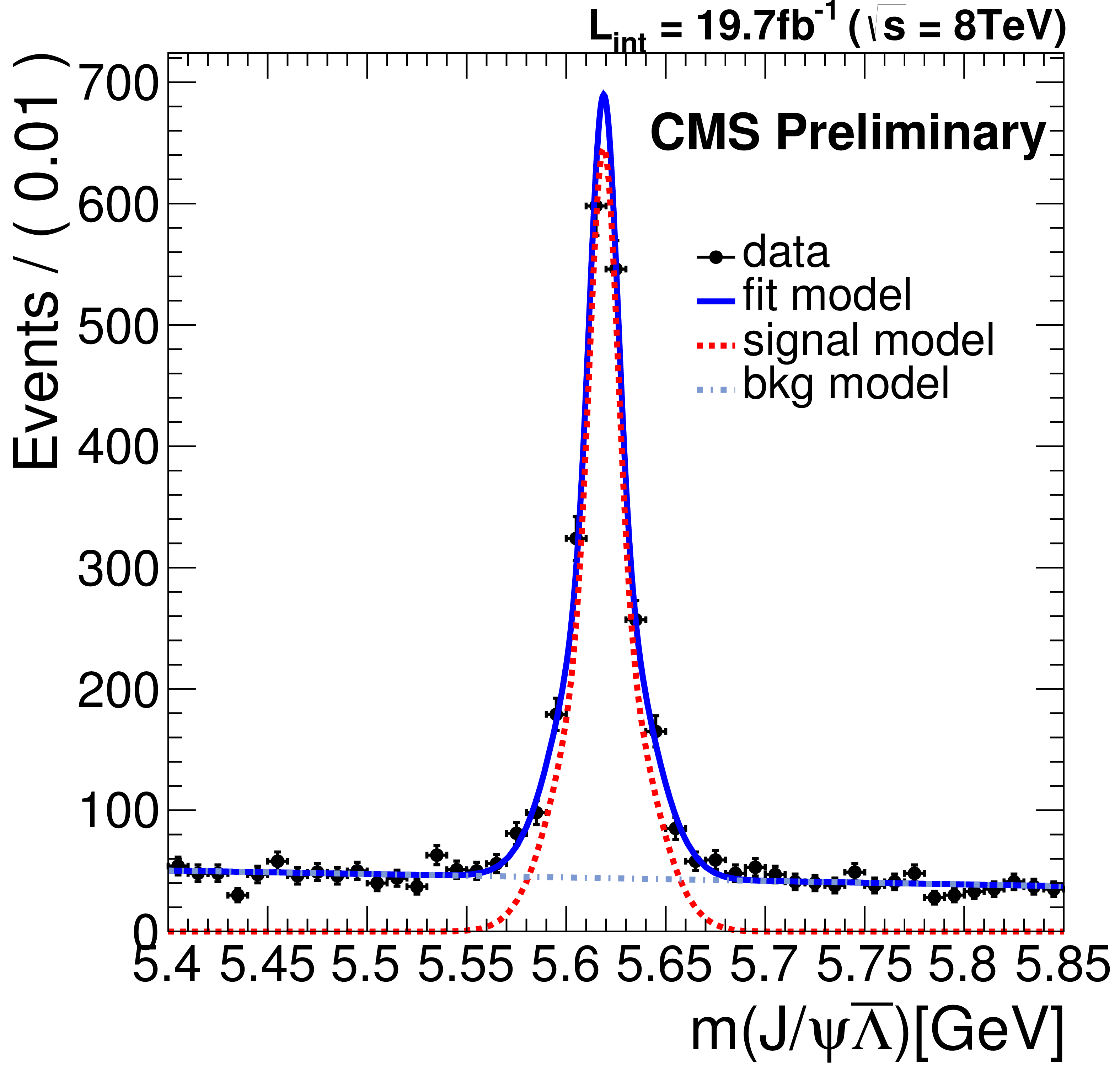
png pdf	Figure 3-b: Invariant mass distribution of $\Lambda_b$ (a and c) and $\overline{\Lambda}_b$ (b and d) candidates in (a-b) 2011 and (c-d) 2012 samples. The solid blue line represents the fit result. The signal (background) projection is shown with a dashed (dot-dashed) red (blue) line.
png pdf	Figure 3-c: Invariant mass distribution of $\Lambda_b$ (a and c) and $\overline{\Lambda}_b$ (b and d) candidates in (a-b) 2011 and (c-d) 2012 samples. The solid blue line represents the fit result. The signal (background) projection is shown with a dashed (dot-dashed) red (blue) line.
png pdf	Figure 3-d: Invariant mass distribution of $\Lambda_b$ (a and c) and $\overline{\Lambda}_b$ (b and d) candidates in (a-b) 2011 and (c-d) 2012 samples. The solid blue line represents the fit result. The signal (background) projection is shown with a dashed (dot-dashed) red (blue) line.
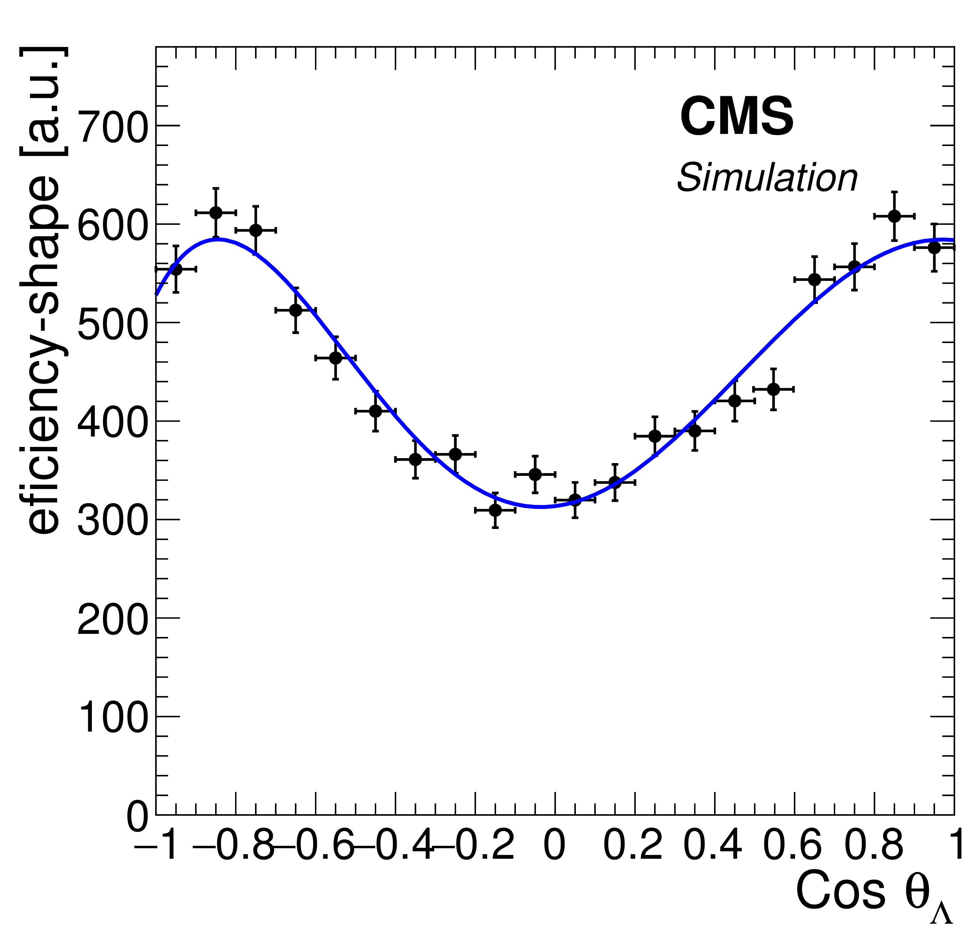
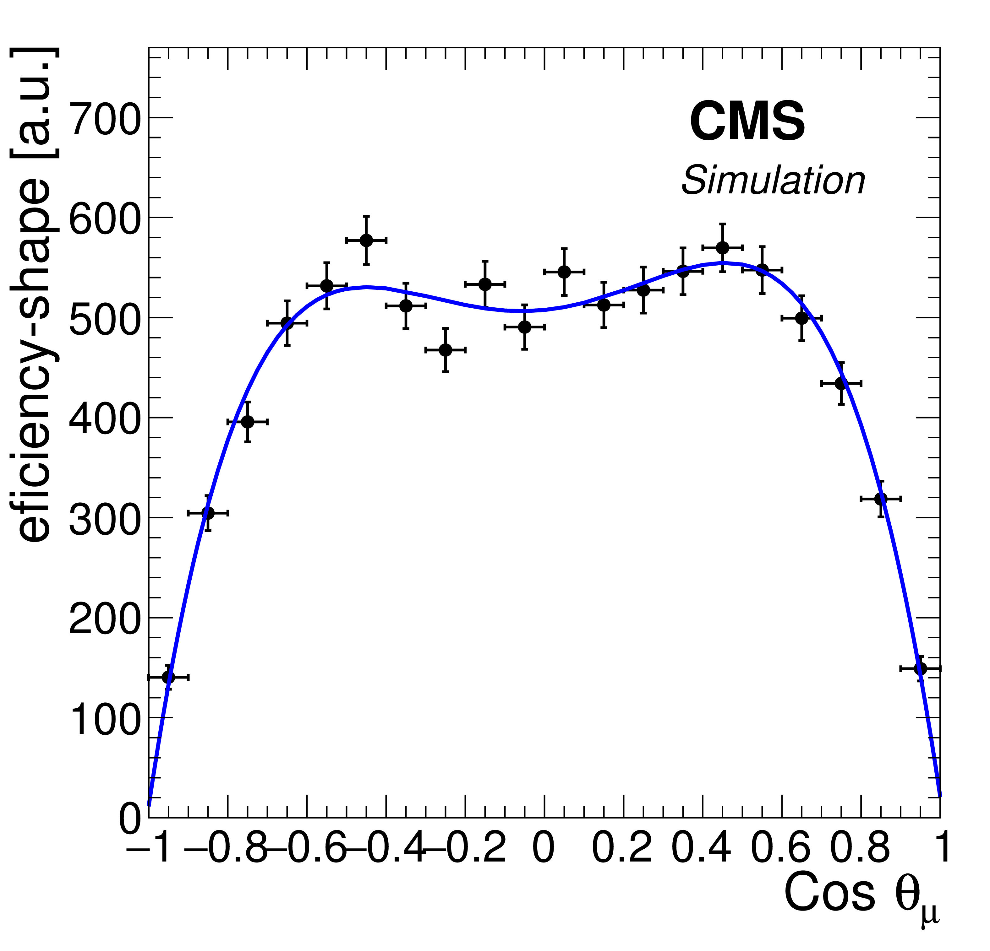
png pdf	Figure 4-a: Angular efficiencies for $\cos\theta _{\Lambda }$, $\cos\theta _{p}$, $\cos\theta _{\mu }$ (from a to c) obtained from simulated $\Lambda _b \rightarrow J/\psi \Lambda ^0$. The angular efficiencies are parametrized with Chebychev polynomials and are fitted simultaneously to the three angular distributions.
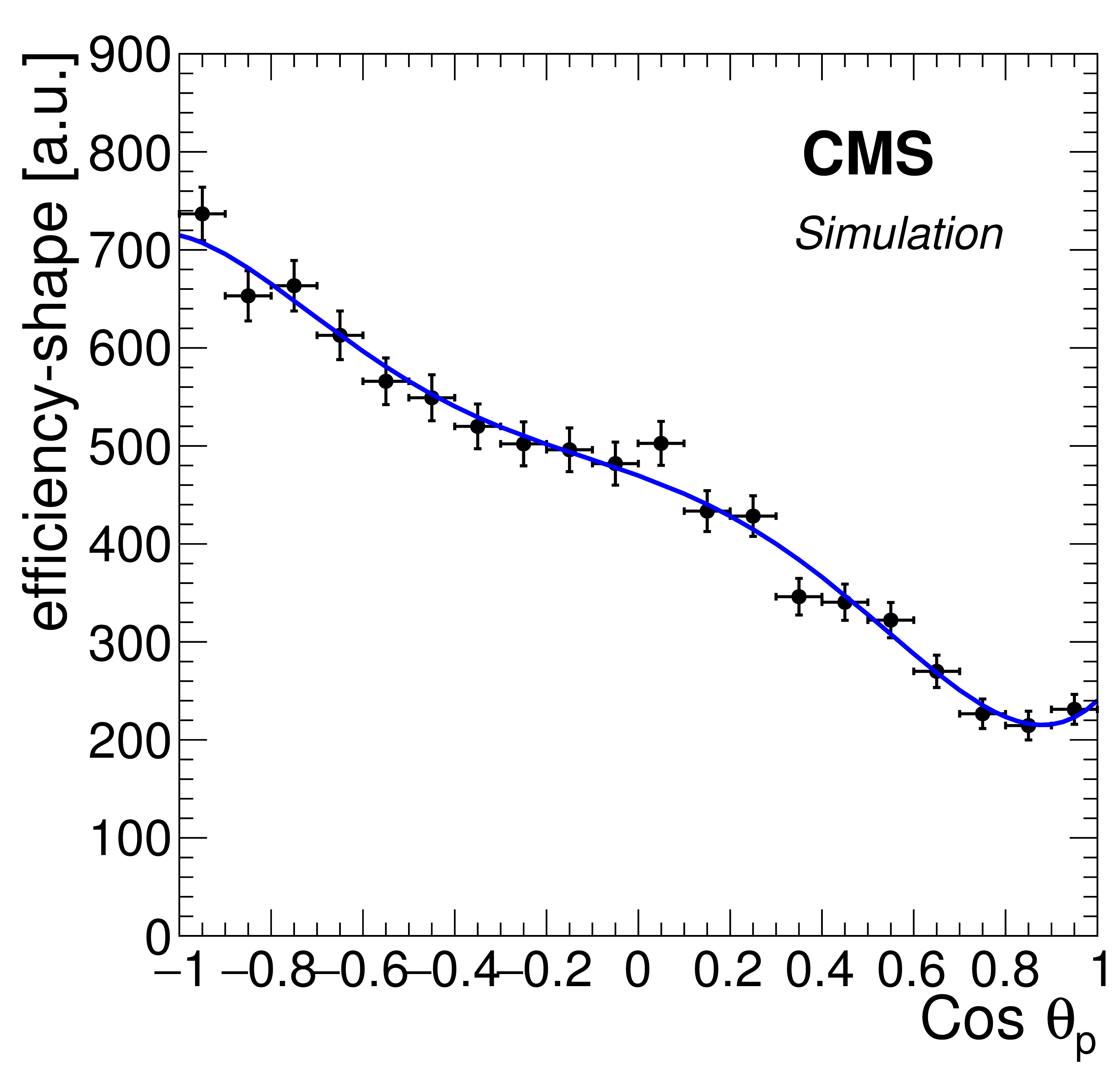
png pdf	Figure 4-b: Angular efficiencies for $\cos\theta _{\Lambda }$, $\cos\theta _{p}$, $\cos\theta _{\mu }$ (from a to c) obtained from simulated $\Lambda _b \rightarrow J/\psi \Lambda ^0$. The angular efficiencies are parametrized with Chebychev polynomials and are fitted simultaneously to the three angular distributions.
png pdf	Figure 4-c: Angular efficiencies for $\cos\theta _{\Lambda }$, $\cos\theta _{p}$, $\cos\theta _{\mu }$ (from a to c) obtained from simulated $\Lambda _b \rightarrow J/\psi \Lambda ^0$. The angular efficiencies are parametrized with Chebychev polynomials and are fitted simultaneously to the three angular distributions.
png pdf	Figure 5-a: Angular background distributions obtained from the mass sidebands are shown from left to right for $\cos\theta _{\Lambda }$, $\cos\theta _{p}$ and $\cos\theta _{\mu }$. The solid blue lines are the results of the fits.
png pdf	Figure 5-b: Angular background distributions obtained from the mass sidebands are shown from left to right for $\cos\theta _{\Lambda }$, $\cos\theta _{p}$ and $\cos\theta _{\mu }$. The solid blue lines are the results of the fits.
png pdf	Figure 5-c: Angular background distributions obtained from the mass sidebands are shown from left to right for $\cos\theta _{\Lambda }$, $\cos\theta _{p}$ and $\cos\theta _{\mu }$. The solid blue lines are the results of the fits.
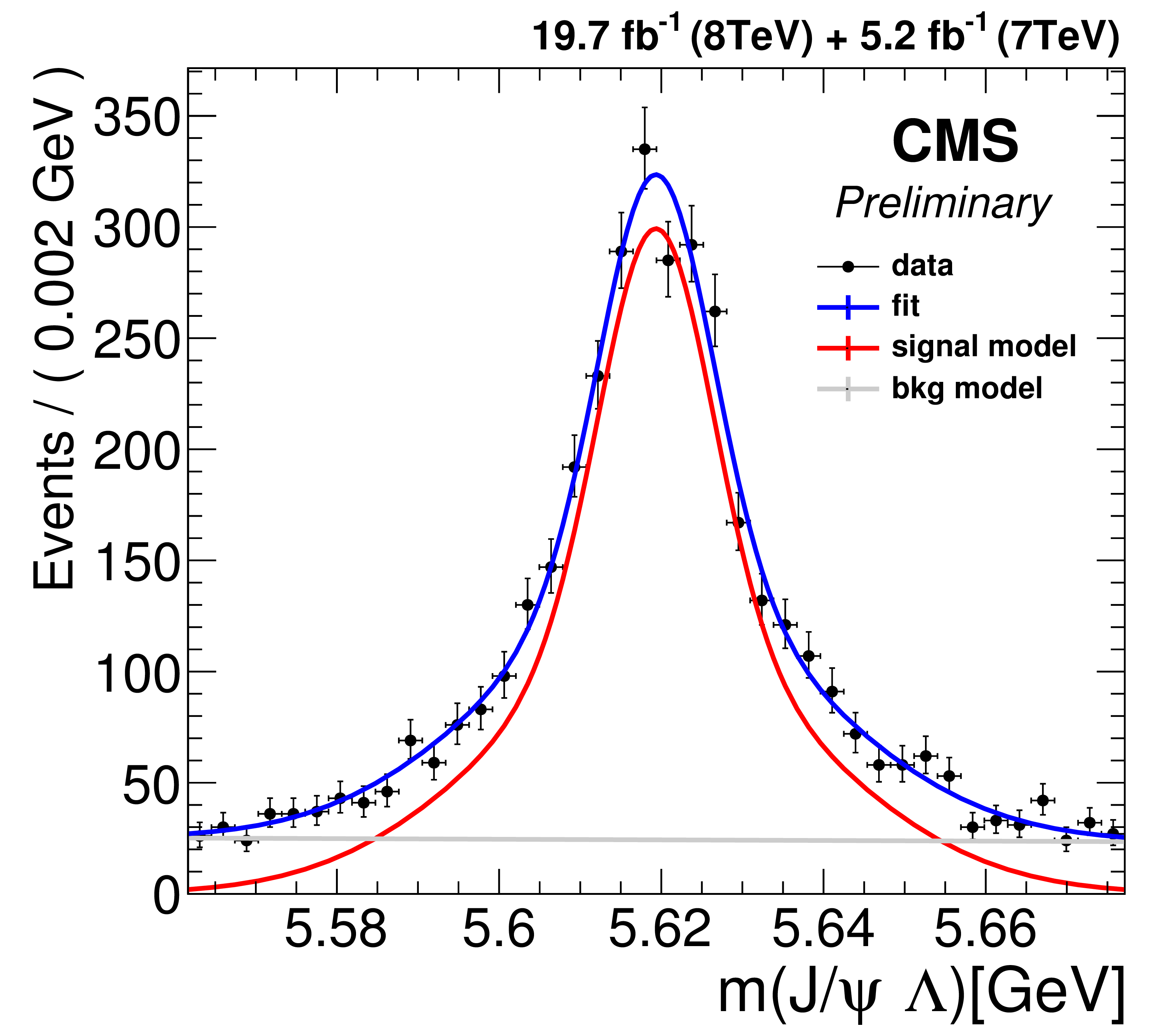
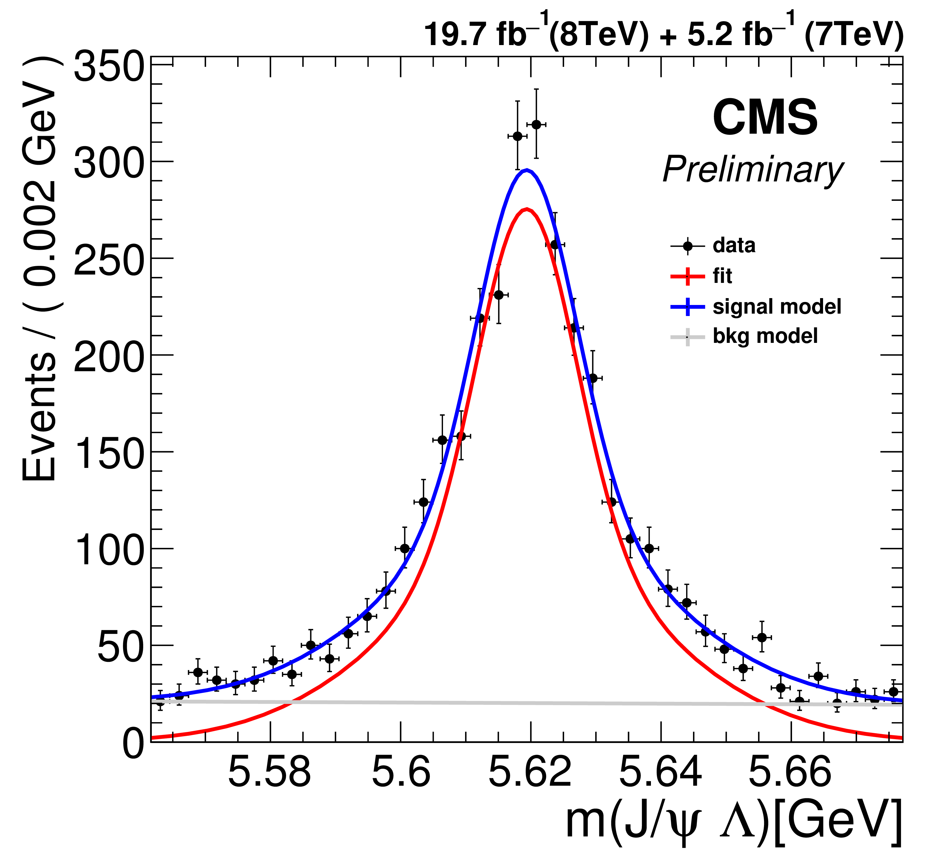
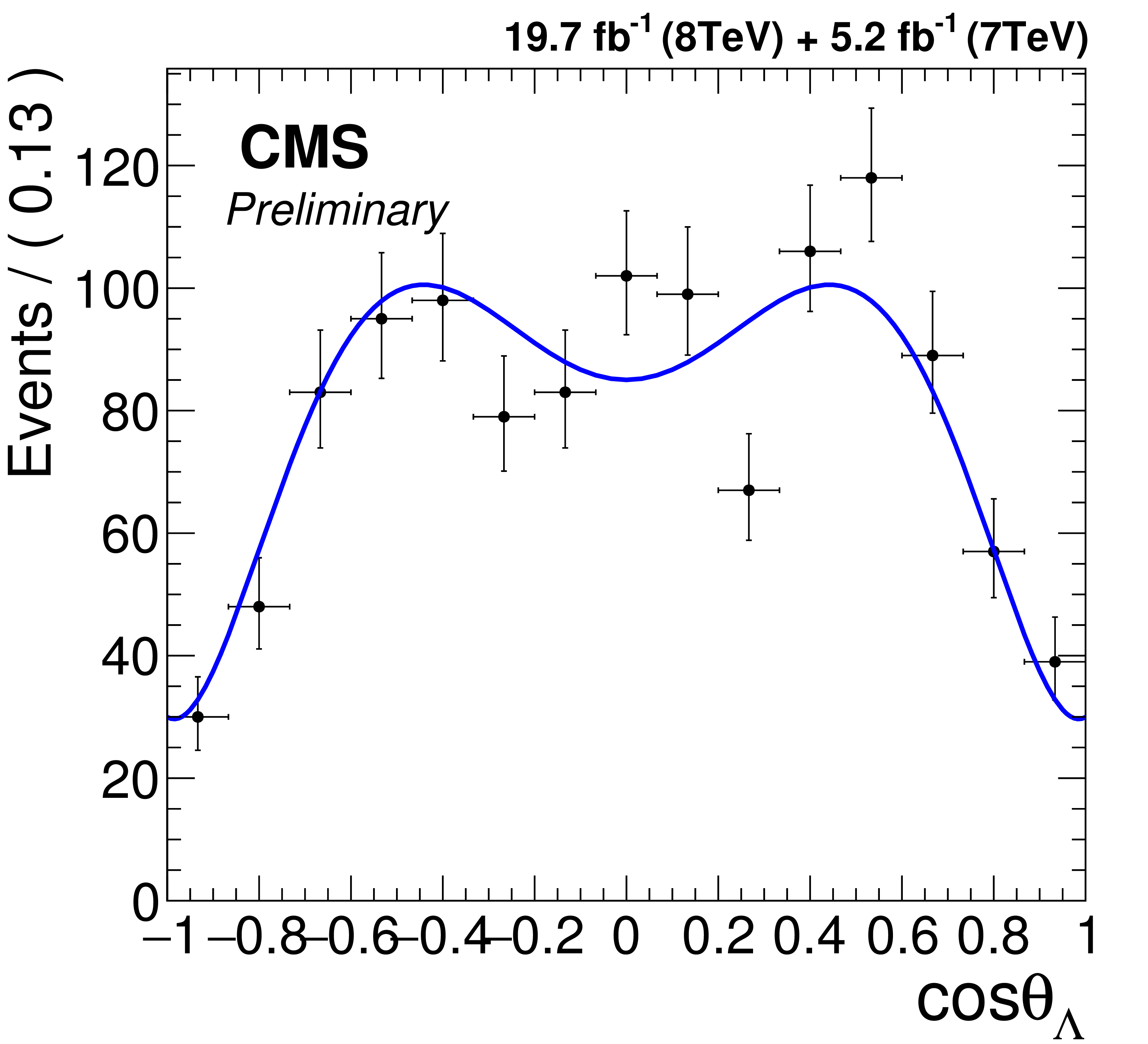
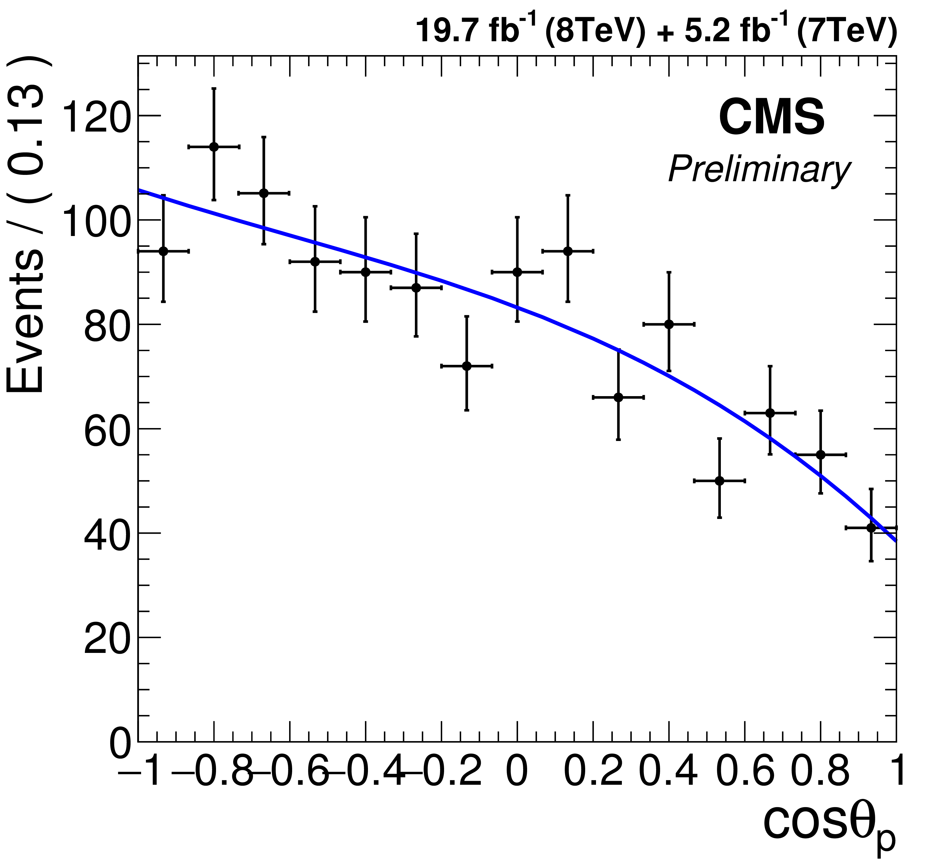
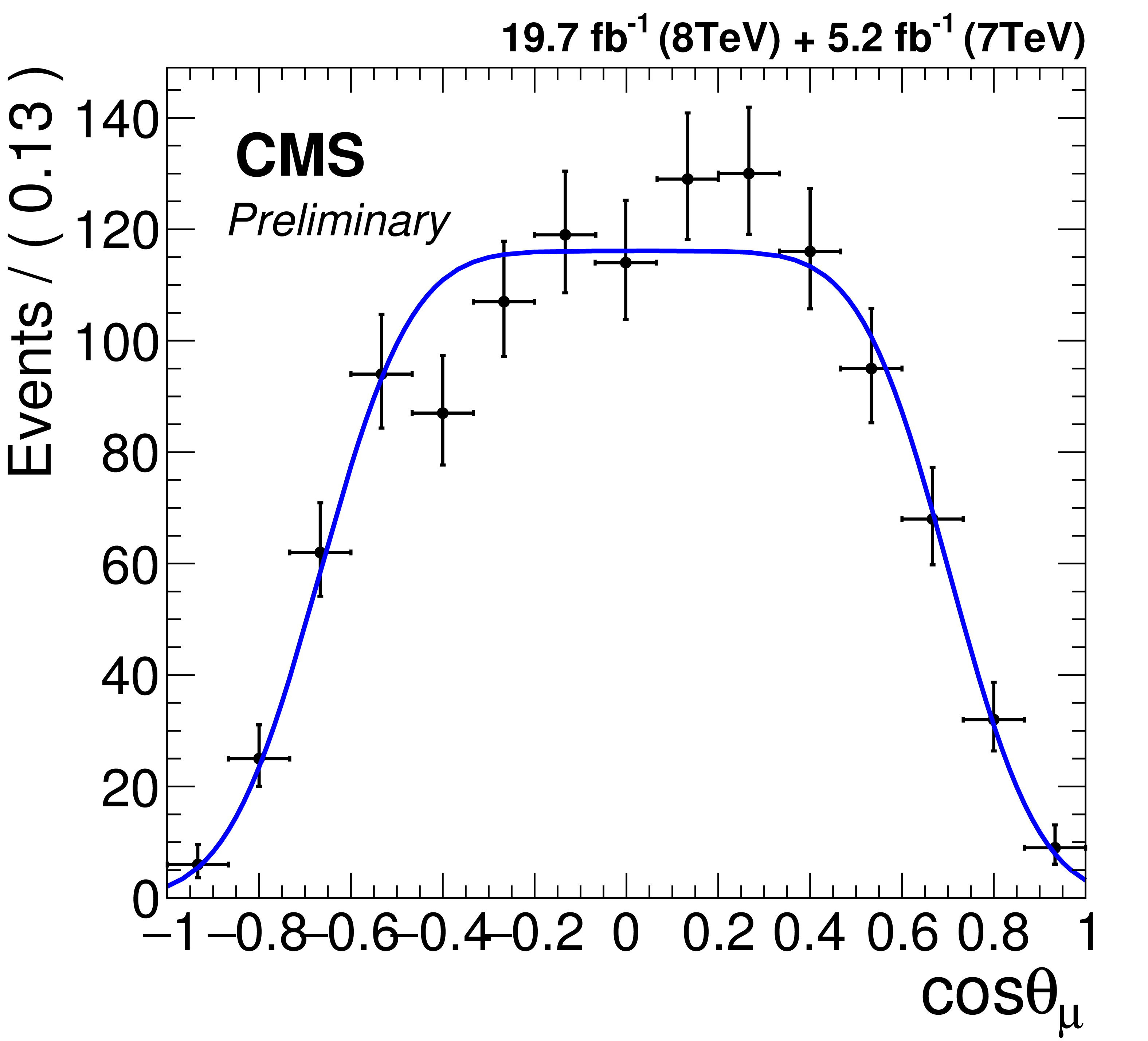
png pdf	Figure 6-a: Distributions of $m(J/\psi \Lambda )$, $\cos\theta _{p}$, $\cos\theta _{\Lambda }$, $\cos\theta _{\mu }$ (from a to d) for $\Lambda _b$ candidates in 2011 and 2012 datasets in $m(J/\psi \Lambda )\in [5.56, 5.68]$, with fit results superimposed. The signal (background) component is shown in red (gray).
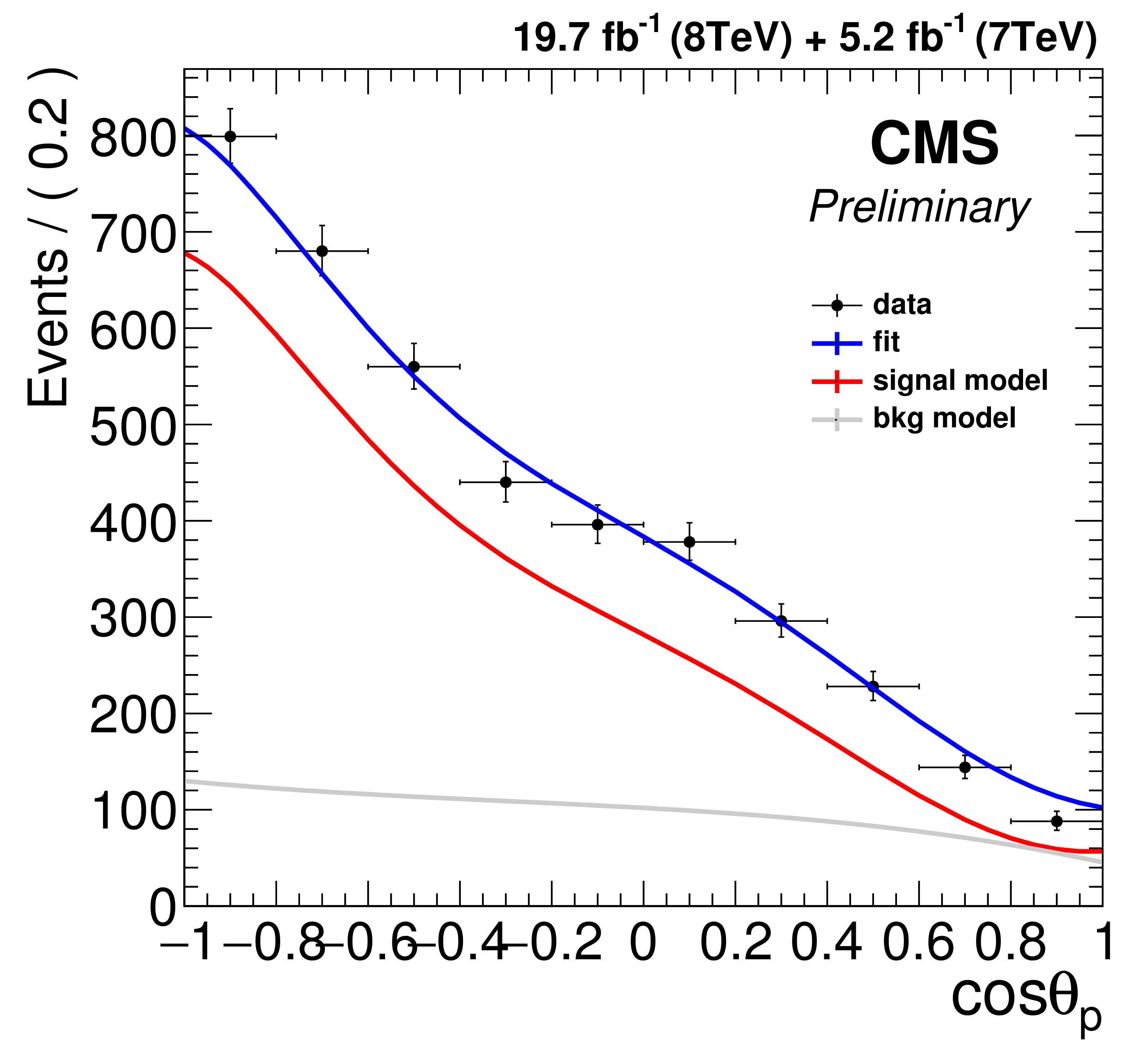
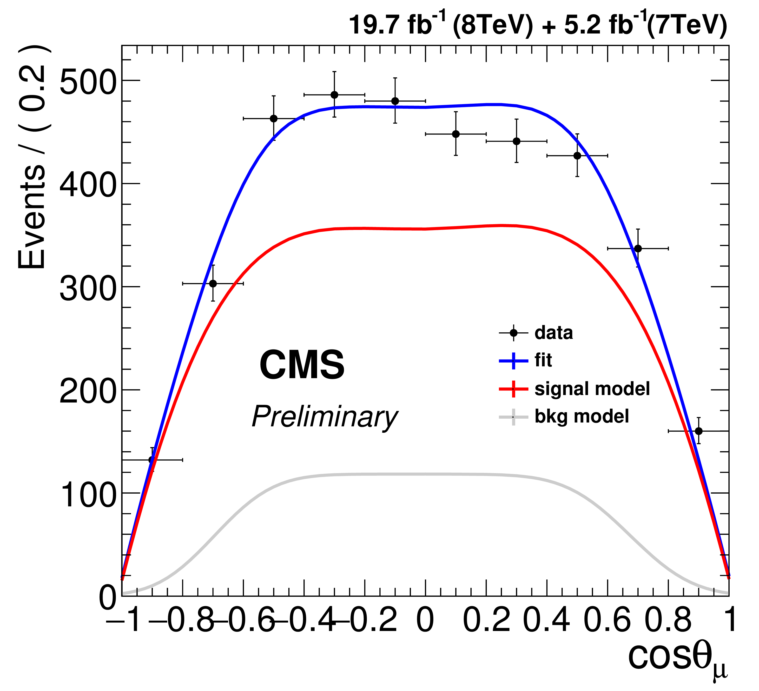
png pdf	Figure 6-b: Distributions of $m(J/\psi \Lambda )$, $\cos\theta _{p}$, $\cos\theta _{\Lambda }$, $\cos\theta _{\mu }$ (from a to d) for $\Lambda _b$ candidates in 2011 and 2012 datasets in $m(J/\psi \Lambda )\in [5.56, 5.68]$, with fit results superimposed. The signal (background) component is shown in red (gray).
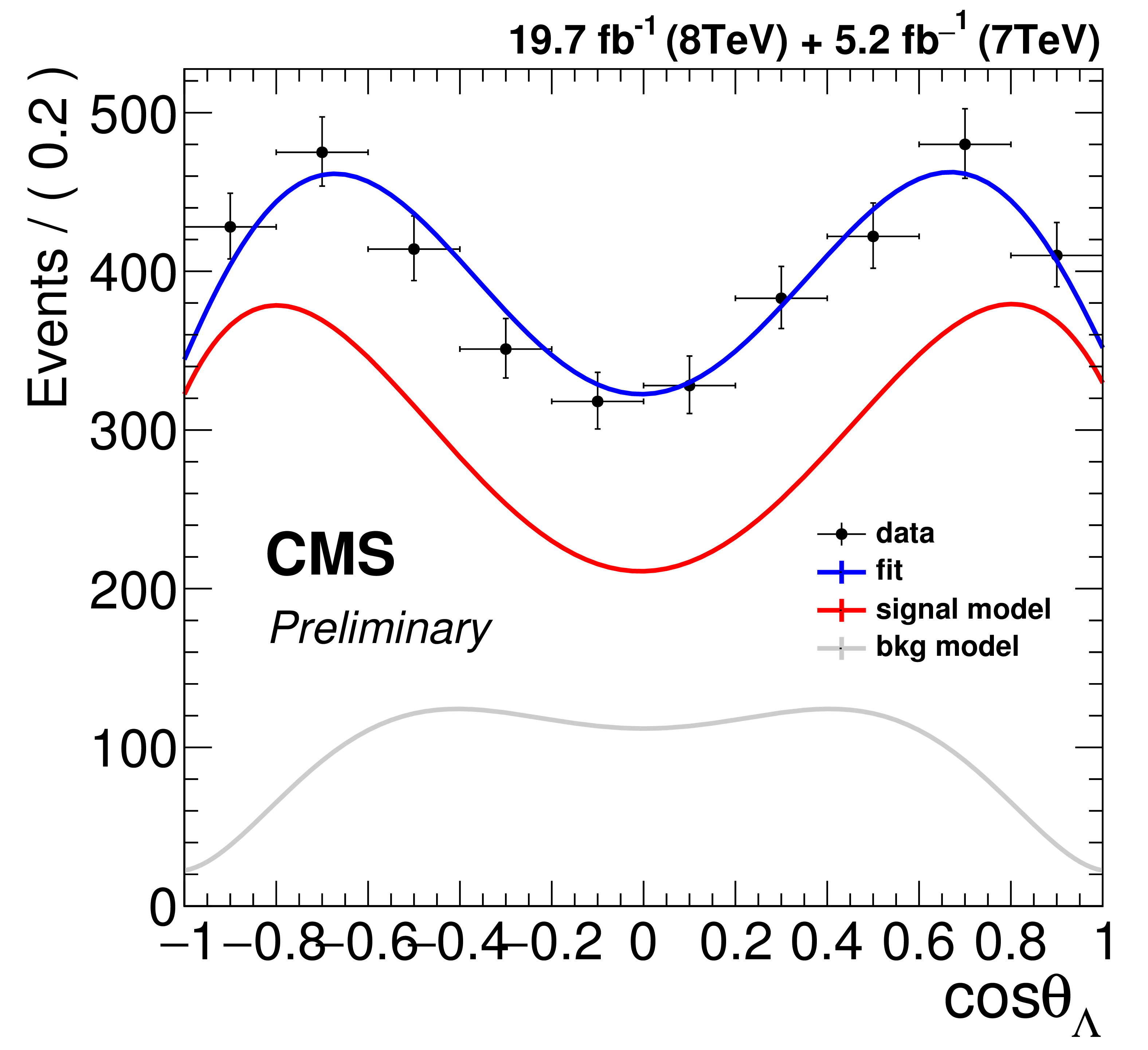
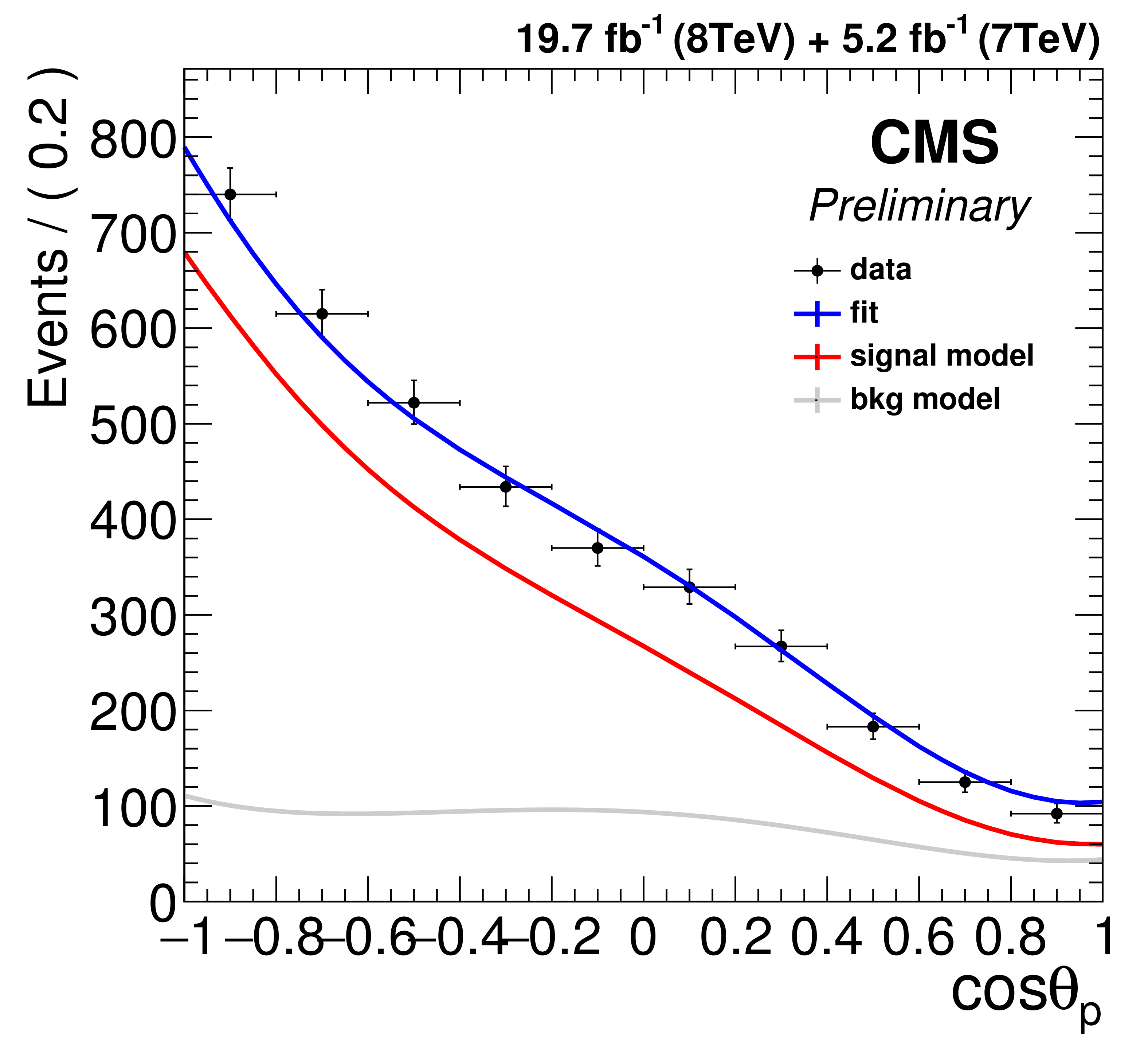
png pdf	Figure 6-c: Distributions of $m(J/\psi \Lambda )$, $\cos\theta _{p}$, $\cos\theta _{\Lambda }$, $\cos\theta _{\mu }$ (from a to d) for $\Lambda _b$ candidates in 2011 and 2012 datasets in $m(J/\psi \Lambda )\in [5.56, 5.68]$, with fit results superimposed. The signal (background) component is shown in red (gray).
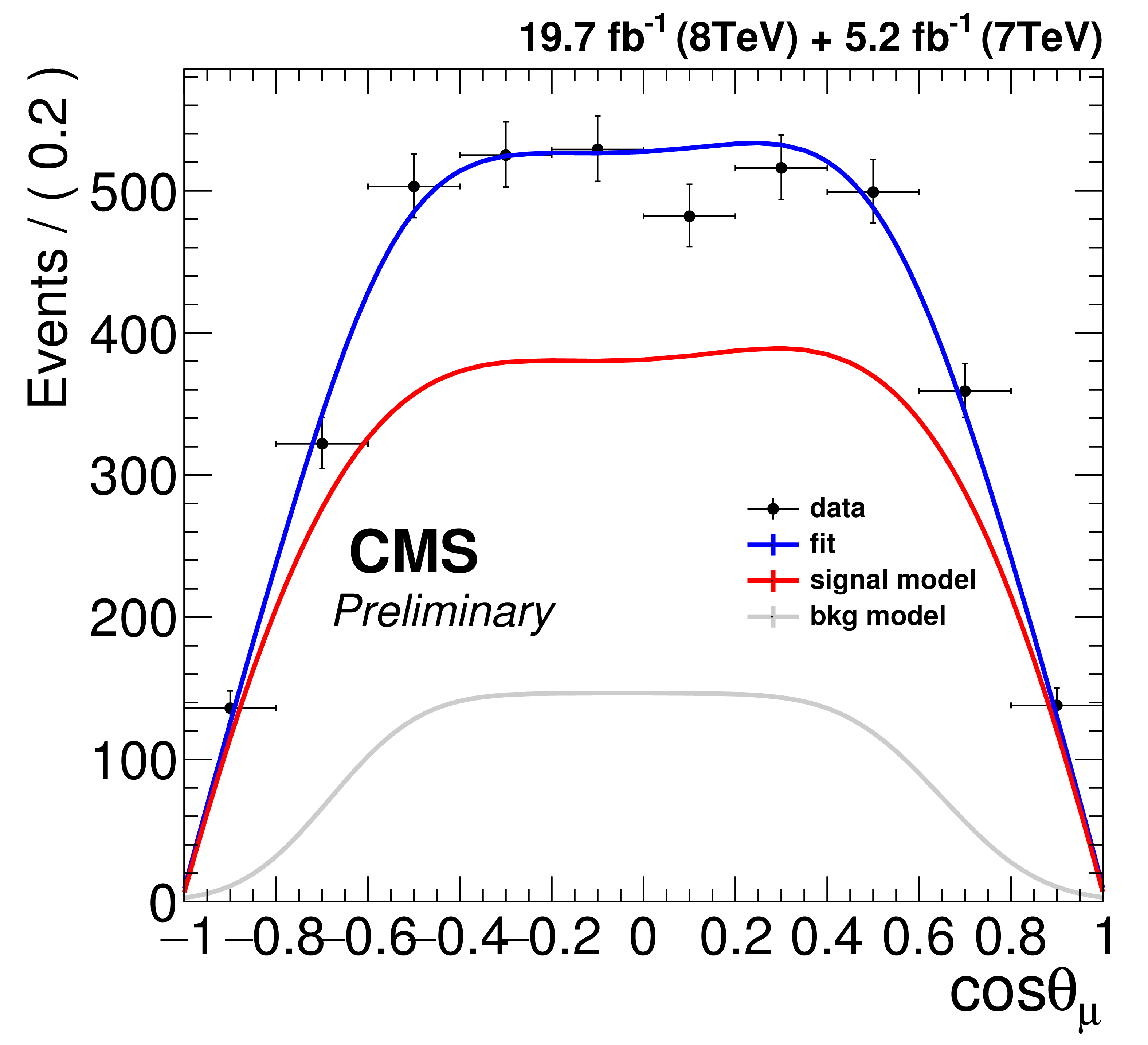
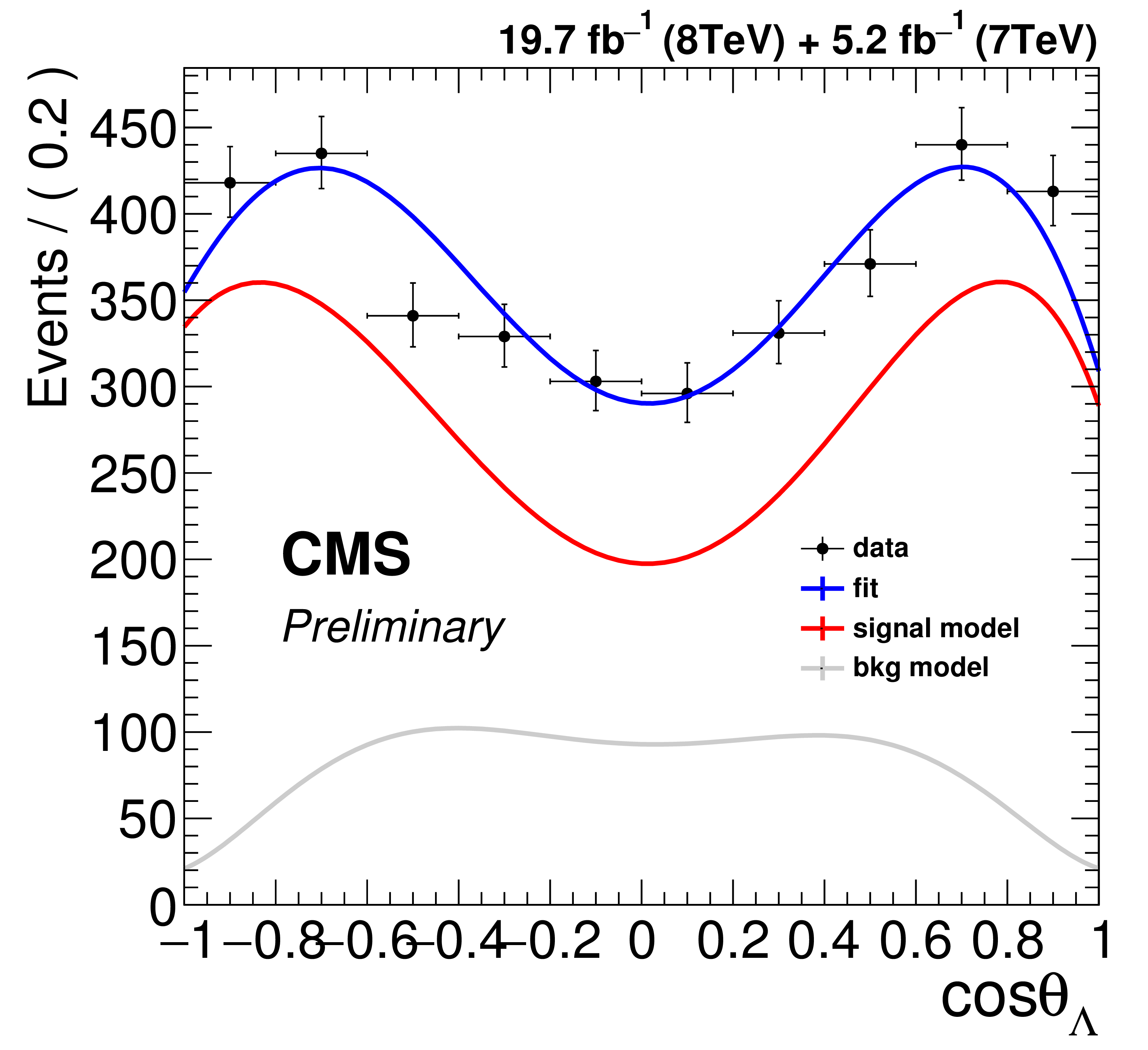
png pdf	Figure 6-d: Distributions of $m(J/\psi \Lambda )$, $\cos\theta _{p}$, $\cos\theta _{\Lambda }$, $\cos\theta _{\mu }$ (from a to d) for $\Lambda _b$ candidates in 2011 and 2012 datasets in $m(J/\psi \Lambda )\in [5.56, 5.68]$, with fit results superimposed. The signal (background) component is shown in red (gray).
png pdf	Figure 7-a: Distributions of $m(J/\psi \overline{\Lambda })$, $\cos\theta _{p}$, $\cos\theta _{\Lambda }$, $\cos\theta _{\mu }$ (from a to d) for $\overline{\Lambda }_b$ candidates in 2011 and 2012 datasets in $m(J/\psi \overline{\Lambda })\in [5.56, 5.68]$, with fit results superimposed. The signal (background) component is shown in red (gray).
png pdf	Figure 7-b: Distributions of $m(J/\psi \overline{\Lambda })$, $\cos\theta _{p}$, $\cos\theta _{\Lambda }$, $\cos\theta _{\mu }$ (from a to d) for $\overline{\Lambda }_b$ candidates in 2011 and 2012 datasets in $m(J/\psi \overline{\Lambda })\in [5.56, 5.68]$, with fit results superimposed. The signal (background) component is shown in red (gray).
png pdf	Figure 7-c: Distributions of $m(J/\psi \overline{\Lambda })$, $\cos\theta _{p}$, $\cos\theta _{\Lambda }$, $\cos\theta _{\mu }$ (from a to d) for $\overline{\Lambda }_b$ candidates in 2011 and 2012 datasets in $m(J/\psi \overline{\Lambda })\in [5.56, 5.68]$, with fit results superimposed. The signal (background) component is shown in red (gray).
png pdf	Figure 7-d: Distributions of $m(J/\psi \overline{\Lambda })$, $\cos\theta _{p}$, $\cos\theta _{\Lambda }$, $\cos\theta _{\mu }$ (from a to d) for $\overline{\Lambda }_b$ candidates in 2011 and 2012 datasets in $m(J/\psi \overline{\Lambda })\in [5.56, 5.68]$, with fit results superimposed. The signal (background) component is shown in red (gray).

Tables
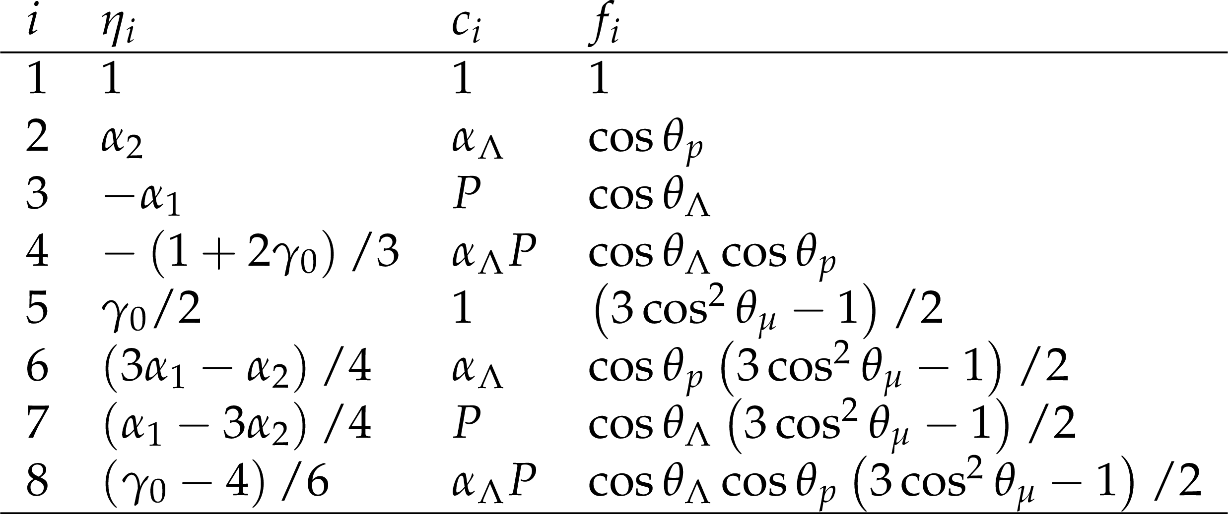
png pdf	Table 1: Functions describing the angular distribution of the decay $\Lambda _{b} \rightarrow J/\psi \Lambda ^{0}$, $J/\psi \rightarrow \mu ^+ \mu ^-$, $\Lambda ^{0} \rightarrow p \pi ^-$.
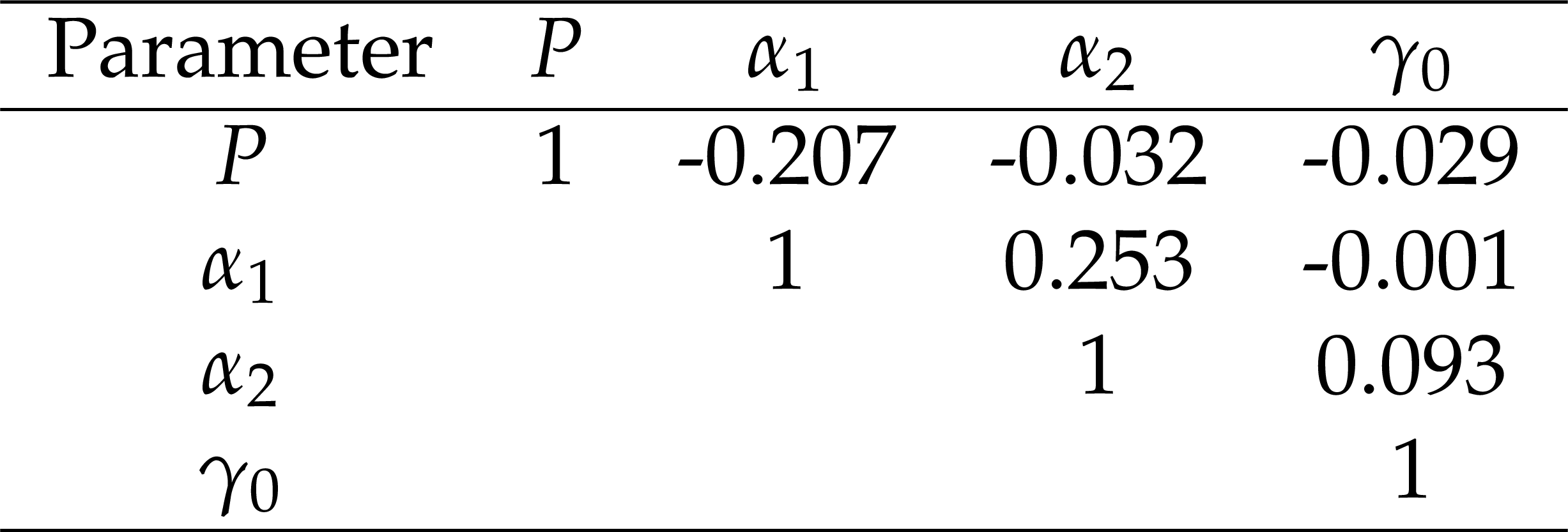
png pdf	Table 2: Correlation Matrix of the fitted parameters.
png pdf	Table 3: Summary of systematic uncertainties.

Summary

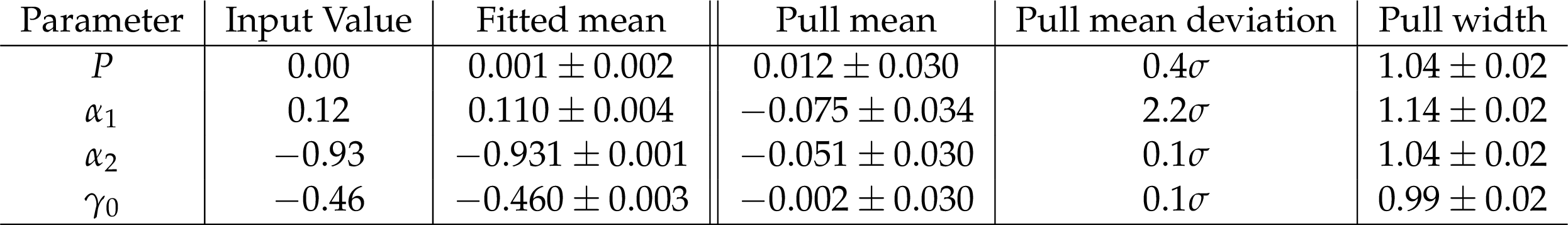
Based on an angular analysis of about 6000 $\Lambda_b \rightarrow J/\psi(\rightarrow\mu^{+}\mu^{-})\Lambda(\rightarrow p\pi^{-})$ decays collected by the CMS experiment in 2011 and 2012, we perform a measurement of the $\Lambda_b$ polarization ($P$), the weak asymmetry parameter of the $\Lambda_b$ decay ($\alpha_1$), the $\Lambda^0$ longitudinal polarization ($\alpha_2$), and a measure of the longitudinal/transverse composition of the $J/\psi$ meson ($\gamma_0$). The measured values are

$P= 0.00 \pm 0.06 \text{(stat)} \pm 0.02 \text{(syst)}$,
$\alpha_1 = 0.12 \pm 0.13 \text{(stat)} \pm 0.06 \text{(syst)}$,
$\alpha_2 = -0.93 \pm 0.04 \text{(stat)} \pm 0.04 \text{(syst)}$,
$\gamma_0 = -0.46 \pm 0.07 \text{(stat)} \pm 0.04 \text{(syst)}$

corresponding to the helicity amplitudes

$ |T_{-0}|^2 = 0.51 \pm 0.03\text{(stat)} \pm 0.02\text{(syst)}$,
$|T_{+0}|^2= -0.02 \pm 0.03\text{(stat)} \pm 0.02\text{(syst)}$,
$|T_{--}|^2= 0.46 \pm 0.02\text{(stat)} \pm 0.02\text{(syst)}$,
$|T_{++}|^2= 0.05 \pm 0.04\text{(stat)} \pm 0.02\text{(syst)}$

Our result of the $\Lambda_b$ polarization is compatible with predictions from perturbative QCD calculations [21] for a polarization of ${\sim}$10% at 1.5$\sigma$, but it disfavors the 20% expectation reported in Ref. [22]. Also, as expected [11], our data analysis indicates a maximum longitudinal $\Lambda^0$ polarization $\alpha_2$, or, equivalently, strongly suppressed transitions into the $\lambda_\Lambda =$ 1/2 helicity states of the $\Lambda$ baryon ($T_{+0}$ and $T_{++}$).

References
1	T. Mannel and G. A. Schuler	Semileptonic decays of bottom baryons at LEP	PLB279 (1992) 194--200
2	A. F. Falk and M. E. Peskin	Production, decay, and polarization of excited heavy hadrons	PRD49 (1994) 3320--3332	hep-ph/9308241
3	ALEPH Collaboration	Measurement of Lambda(b) polarization in Z decays	PLB365 (1996) 437--447
4	OPAL Collaboration	Measurement of the average polarization of b baryons in hadronic Z0 decays	PLB444 (1998) 539--554	hep-ex/9808006
5	DELPHI Collaboration	Lambda(b) polarization in Z0 decays at LEP	PLB474 (2000) 205--222
6	B. Mele and G. Altarelli	Lepton spectra as a measure of b quark polarization at LEP	PLB299 (1993) 345--350
7	LHCb Collaboration	Measurements of the $ \Lambda_b^0 \to J/\psi \Lambda $ decay amplitudes and the $ \Lambda_b^0 $ polarisation in $ pp $ collisions at $ \sqrt{s} = 7 $ TeV	PLB724 (2013) 27--35	1302.5578
8	CMS Collaboration	The CMS experiment at the CERN LHC	JINST 3 (2008) S08004	CMS-00-001
9	P. Bialas, J. G. Korner, M. Kramer, and K. Zalewski	Joint angular decay distributions in exclusive weak decays of heavy mesons and baryons	Z. Phys. C57 (1993) 115--134
10	M. Kramer and H. Simma	Angular correlations in $ \Lambda_{b}\to\Lambda+V $: Polarization measurements, HQET and CP violation	NPPS 50 (1996) 125--129, .[125(1996)]
11	T. Gutsche et al.	Polarization effects in the cascade decay $ { {\Lambda}}_{b} {\rightarrow} {\Lambda}\mathbf{(} {\rightarrow}p{ {\pi}}^{\mathbf{-}}\mathbf{)}\mathbf{+}J/ {\psi}\mathbf{(} {\rightarrow}{ {\ell}}^{\mathbf{+}}{ {\ell}}^{\mathbf{-}}\mathbf{)} $ in the covariant confined quark model	PRD 88 (Dec, 2013) 114018
12	Particle Data Group Collaboration	Review of Particle Physics	CPC38 (2014) 090001
13	T. Sjostrand, S. Mrenna, and P. Z. Skands	PYTHIA 6.4 Physics and Manual	JHEP 05 (2006) 026	hep-ph/0603175
14	D. J. Lange	The EvtGen particle decay simulation package	NIMA462 (2001) 152--155
15	M. Brun, R. Hagelberg, and J. Lassalle	GEANT1	CERN-DD-78-2-REV
16	E. Gerchtein and M. Paulini	CDF detector simulation framework and performance	2003
17	M. I. Rikova	Measurement of the $\Lambda_b$ Polarization with pp Collisions at 7 TeV	CERN-THESIS-2013-218
18	CMS Collaboration	Measurement of differential cross sections versus $p_{\mathrm{T}}$ and $\|y\|$ of $K_0^S$, $\Lambda^0$ and $\Xi^-$ from 7 TeV pp collisions at CMS	CMS-AN-10-084
19	W. Verkerke	The RooFit toolkit for data modelling	eConf C0303241, CHEP03 2003
20	ATLAS Collaboration	Measurement of the parity-violating asymmetry parameter $ { {\alpha}}_{b} $ and the helicity amplitudes for the decay $ { {\Lambda}}_{b}^{0} {\rightarrow}J/ {\psi}{ {\Lambda}}^{0} $ with the ATLAS detector	PRD 89 (May, 2014) 092009
21	G. Hiller, M. Knecht, F. Legger, and T. Schietinger	Photon polarization from helicity suppression in radiative decays of polarized Lambda(b) to spin-3/2 baryons	PLB649 (2007) 152--158	hep-ph/0702191
22	Z. J. Ajaltouni, E. Conte, and O. Leitner	$ \Lambda_{b}^{0} $ decays into $ \Lambda -vector $	PLB614 (2005) 165--173	hep-ph/0412116