

Compact Muon Solenoid
LHC, CERN
| CMS-PAS-B2G-16-004 | ||
| Search for WW in semileptonic final states: low mass extension | ||
| CMS Collaboration | ||
| March 2016 | ||
| Abstract: A search for massive narrow resonances decaying to pairs of W bosons is presented, based on 2.3 fb$^{-1}$ of pp collision data collected by the CMS experiment at the CERN LHC with a centre-of-mass energy of 13 TeV. Resonances corresponding to masses in the range [600-1000] GeV and decaying through WW pairs to $ \ell \nu \mathrm{qq} $ are probed. Cross section and resonance mass exclusion limits are set for models that predict gravitons. | ||
|
Links:
CDS record (PDF) ;
CADI line (restricted) ;
These preliminary results are superseded in this paper, JHEP 03 (2017) 162. The superseded preliminary plots can be found here. |
||
| Figures | |
png pdf |
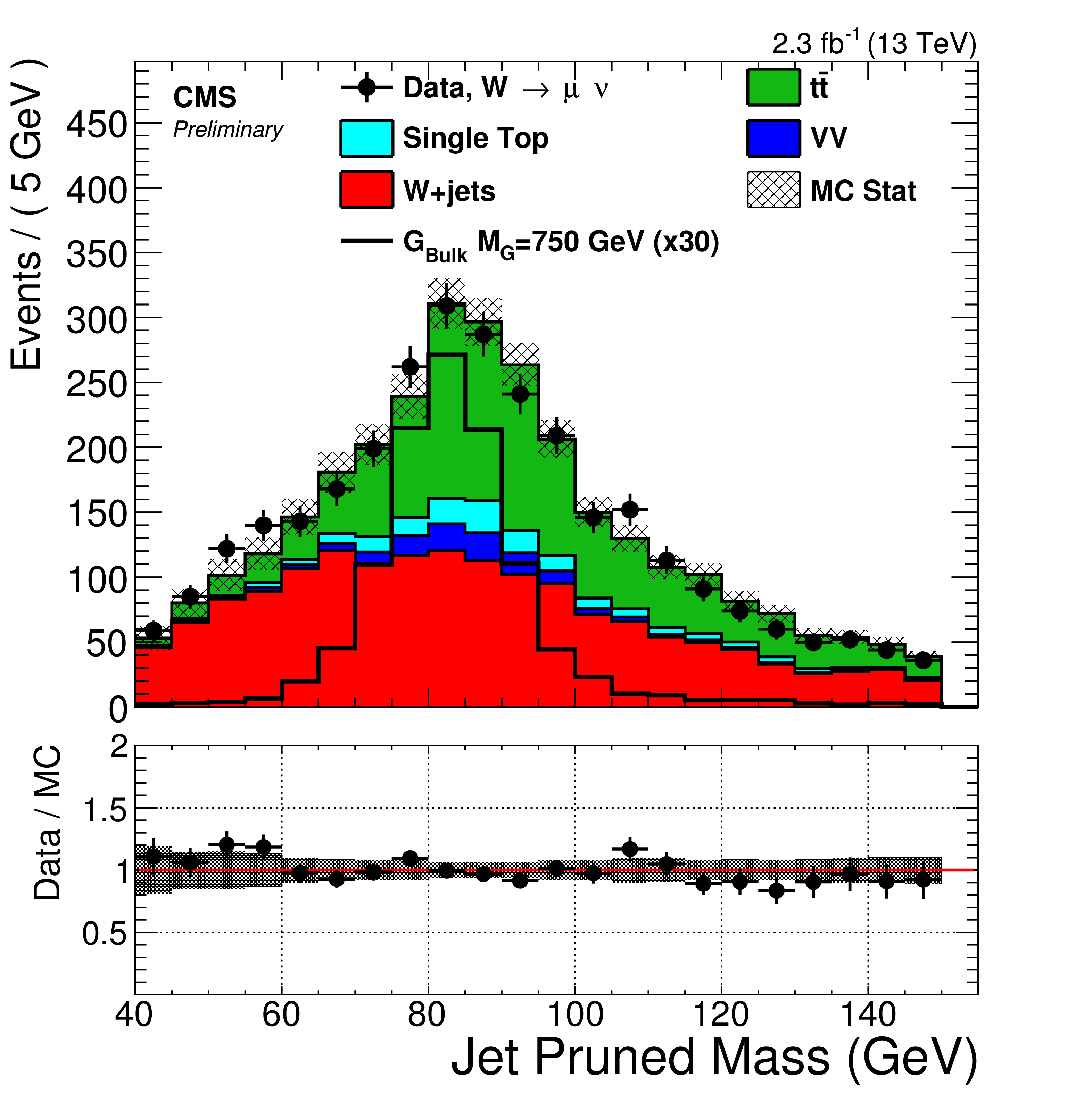
Figure 1-a:
Pruned jet mass and $N$-subjettiness ratio $\tau _{21}$ distributions in the $M_{J}$ signal region and sideband. The signal distributions are scaled to an arbitrary cross section for better visualisation. The W+jets background from simulation is rescaled such that the total number of background events matches the number of events in data. The grey band represents the statistical uncertainty. a,b: muon channel, c,d: electron channel. |
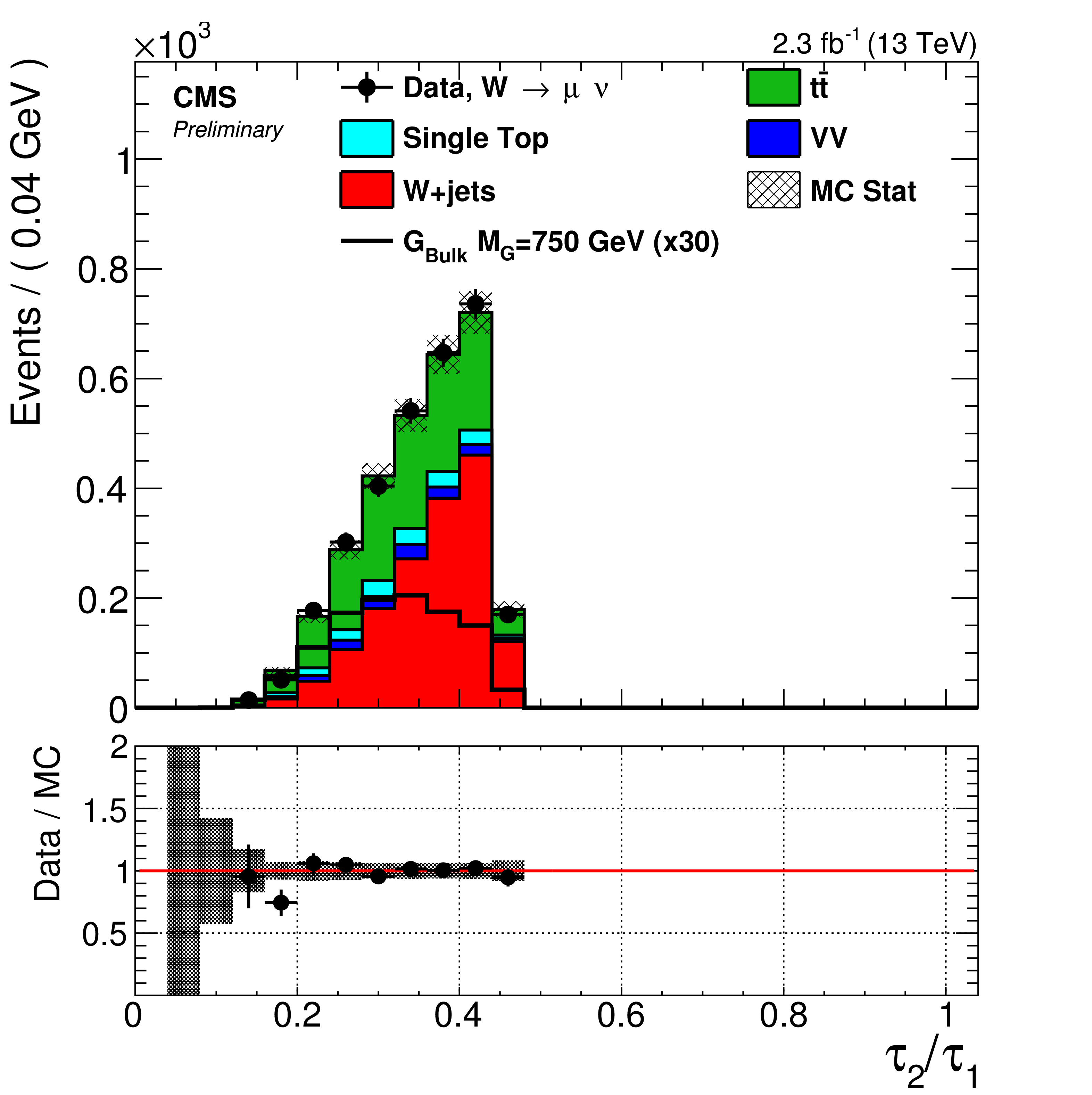
png pdf |
Figure 1-b:
Pruned jet mass and $N$-subjettiness ratio $\tau _{21}$ distributions in the $M_{J}$ signal region and sideband. The signal distributions are scaled to an arbitrary cross section for better visualisation. The W+jets background from simulation is rescaled such that the total number of background events matches the number of events in data. The grey band represents the statistical uncertainty. a,b: muon channel, c,d: electron channel. |

png pdf |
Figure 1-c:
Pruned jet mass and $N$-subjettiness ratio $\tau _{21}$ distributions in the $M_{J}$ signal region and sideband. The signal distributions are scaled to an arbitrary cross section for better visualisation. The W+jets background from simulation is rescaled such that the total number of background events matches the number of events in data. The grey band represents the statistical uncertainty. a,b: muon channel, c,d: electron channel. |

png pdf |
Figure 1-d:
Pruned jet mass and $N$-subjettiness ratio $\tau _{21}$ distributions in the $M_{J}$ signal region and sideband. The signal distributions are scaled to an arbitrary cross section for better visualisation. The W+jets background from simulation is rescaled such that the total number of background events matches the number of events in data. The grey band represents the statistical uncertainty. a,b: muon channel, c,d: electron channel. |

png pdf |
Figure 2-a:
Distributions of the pruned jet mass $ {m_{\text {jet}}}$ in the muon (a) and electron (b) channels. The uncertainty band represents the statistical uncertainty on the background prediction. All selections are applied except the final $ {m_{\text {jet}}}$ signal window requirement. Data are shown as black markers. The contribution of the W+jets background is extrapolated from the sideband to the signal region 65-95 GeV, which is represented with a grey shaded area and marked with a label. The grey shaded area between 95-135 GeV is not used in the analysis in order to avoid bias in future searches for WH, ZH and HH resonances. |

png pdf |
Figure 2-b:
Distributions of the pruned jet mass $ {m_{\text {jet}}}$ in the muon (a) and electron (b) channels. The uncertainty band represents the statistical uncertainty on the background prediction. All selections are applied except the final $ {m_{\text {jet}}}$ signal window requirement. Data are shown as black markers. The contribution of the W+jets background is extrapolated from the sideband to the signal region 65-95 GeV, which is represented with a grey shaded area and marked with a label. The grey shaded area between 95-135 GeV is not used in the analysis in order to avoid bias in future searches for WH, ZH and HH resonances. |
png pdf |
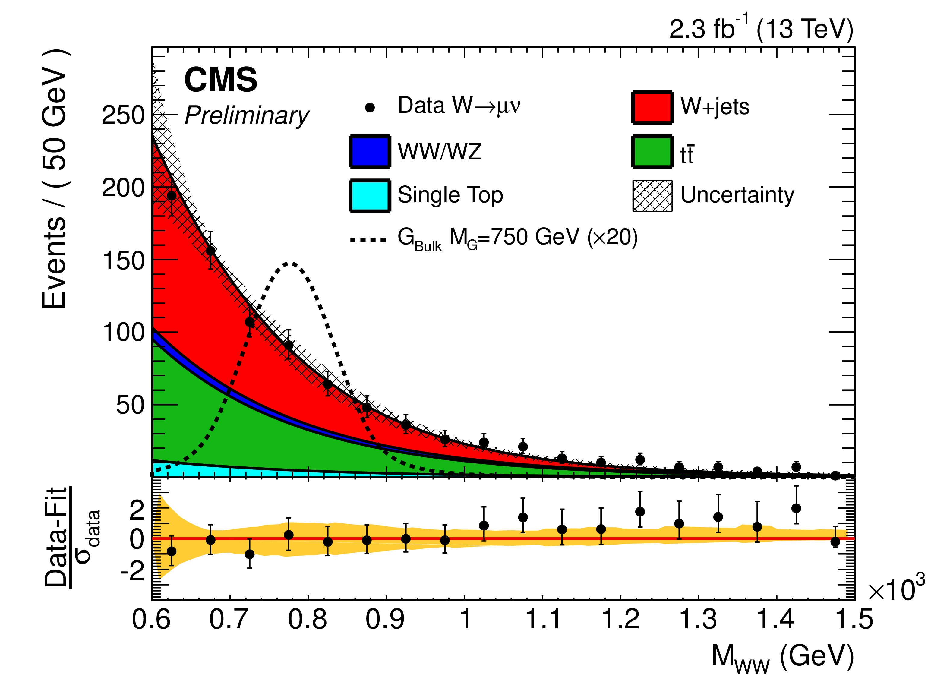
Figure 3-a:
Final observed $ {m_{\mathrm{ W } \mathrm{ W } }} $ distributions for the WW analyses in the signal region. a: Muon channel. b: Electron channel. c: Muon and electron channels combined together. The solid curve represents the background estimation provided by the alpha method. The hatched band includes both statistical and systematics (of normalization and of shape) uncertainties. The data are shown as black markers. The bottom panels show the corresponding pull distributions, quantifying the agreement between the background-only hypothesis and the data. The pull distribution is defined as the difference between the data and the background prediction, divided by the error on data. The error bars on the points represent the error on data, while the uncertainty band (statistics+systematics) on the background prediction is shown with a yellow band. |
png pdf |
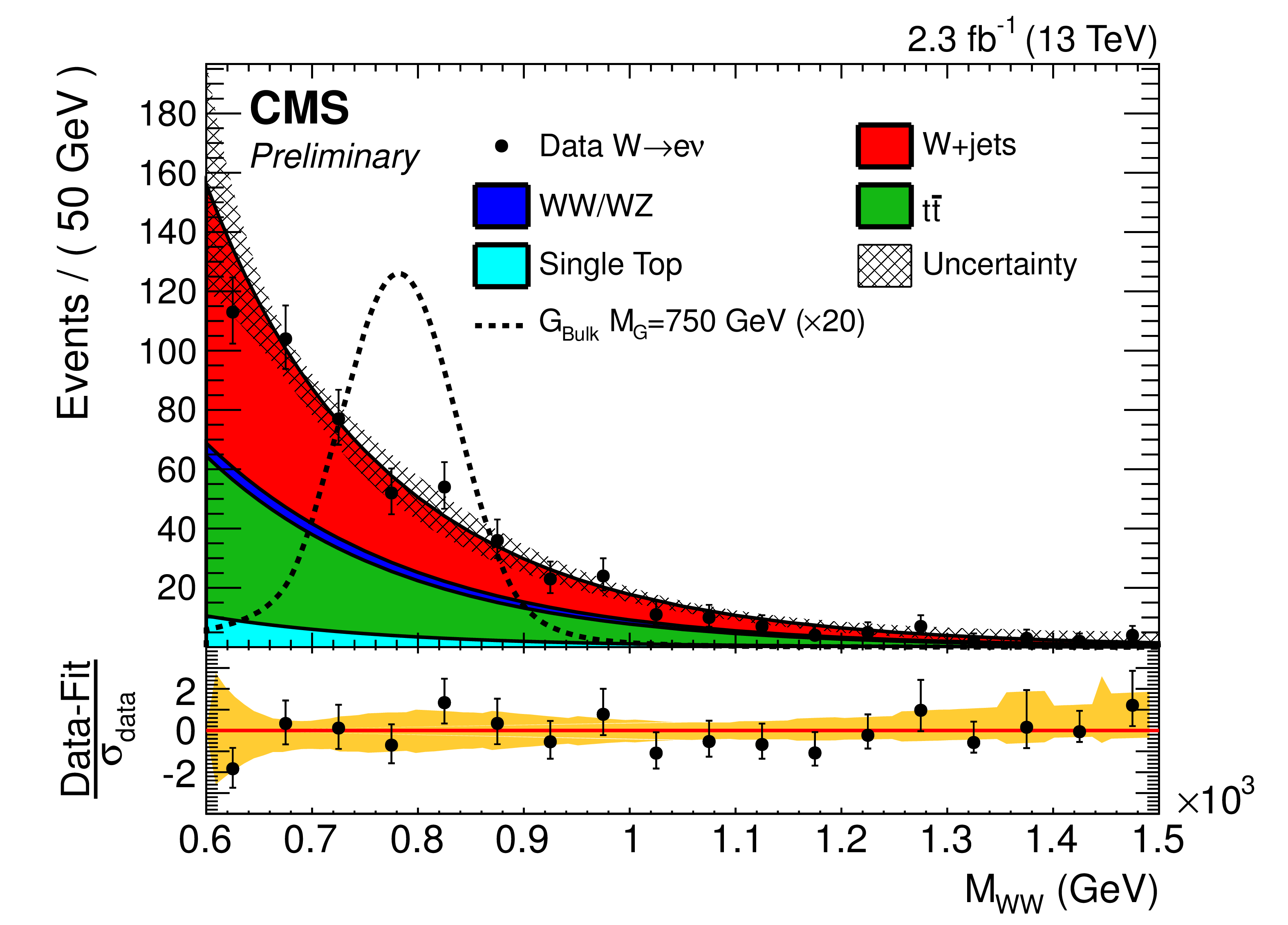
Figure 3-b:
Final observed $ {m_{\mathrm{ W } \mathrm{ W } }} $ distributions for the WW analyses in the signal region. a: Muon channel. b: Electron channel. c: Muon and electron channels combined together. The solid curve represents the background estimation provided by the alpha method. The hatched band includes both statistical and systematics (of normalization and of shape) uncertainties. The data are shown as black markers. The bottom panels show the corresponding pull distributions, quantifying the agreement between the background-only hypothesis and the data. The pull distribution is defined as the difference between the data and the background prediction, divided by the error on data. The error bars on the points represent the error on data, while the uncertainty band (statistics+systematics) on the background prediction is shown with a yellow band. |

png pdf |
Figure 3-c:
Final observed $ {m_{\mathrm{ W } \mathrm{ W } }} $ distributions for the WW analyses in the signal region. a: Muon channel. b: Electron channel. c: Muon and electron channels combined together. The solid curve represents the background estimation provided by the alpha method. The hatched band includes both statistical and systematics (of normalization and of shape) uncertainties. The data are shown as black markers. The bottom panels show the corresponding pull distributions, quantifying the agreement between the background-only hypothesis and the data. The pull distribution is defined as the difference between the data and the background prediction, divided by the error on data. The error bars on the points represent the error on data, while the uncertainty band (statistics+systematics) on the background prediction is shown with a yellow band. |
png pdf |
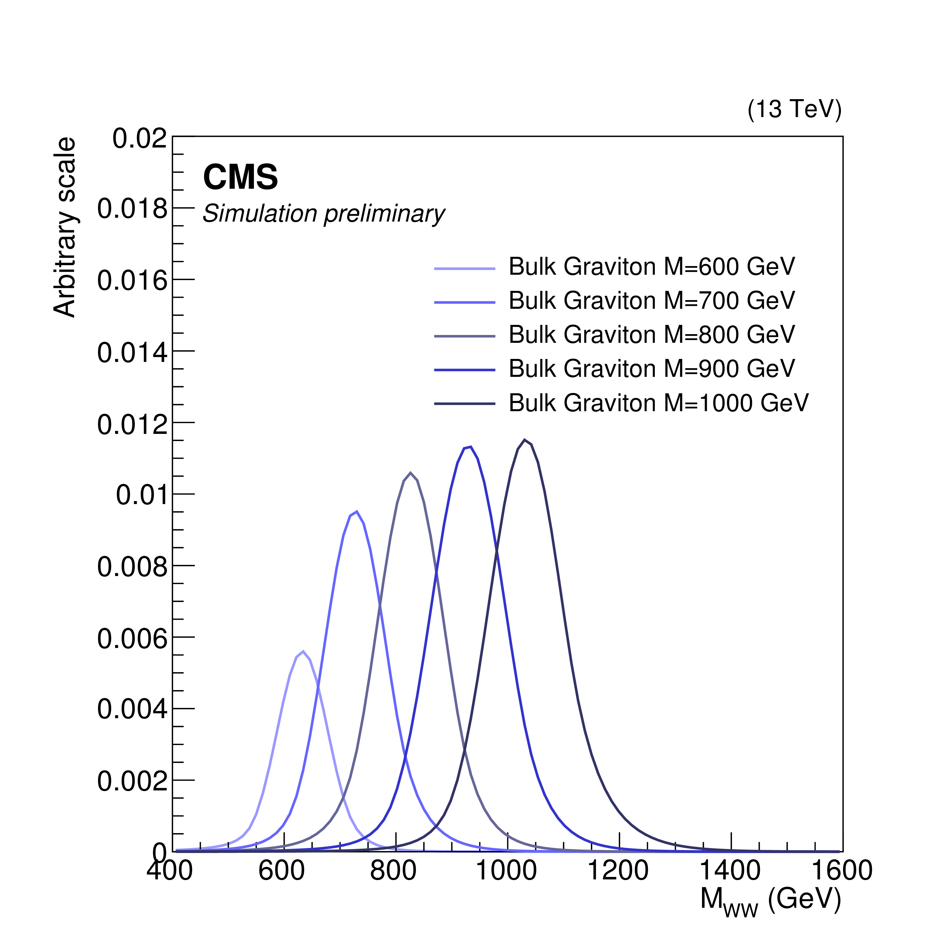
Figure 4:
$M_{\mathrm{ WW } }$ distribution for different signal mass points. The area of each shape is proportional to the total signal efficiency of the corresponding mass point. |

png pdf |
Figure 5-a:
Observed (black solid) and expected (black dashed) 95% CL upper limits on the product of the graviton production cross section and the branching fraction of $ {\mathrm{G} _{\mathrm {bulk}}}\to \mathrm{ W } \mathrm{ W } $ in the muon (a) and electron (b) channel. The theoretical cross section multiplied by the relevant branching ratio is shown as a red solid line. |

png pdf |
Figure 5-b:
Observed (black solid) and expected (black dashed) 95% CL upper limits on the product of the graviton production cross section and the branching fraction of $ {\mathrm{G} _{\mathrm {bulk}}}\to \mathrm{ W } \mathrm{ W } $ in the muon (a) and electron (b) channel. The theoretical cross section multiplied by the relevant branching ratio is shown as a red solid line. |

png pdf |
Figure 6:
|
| Tables | |
png pdf |
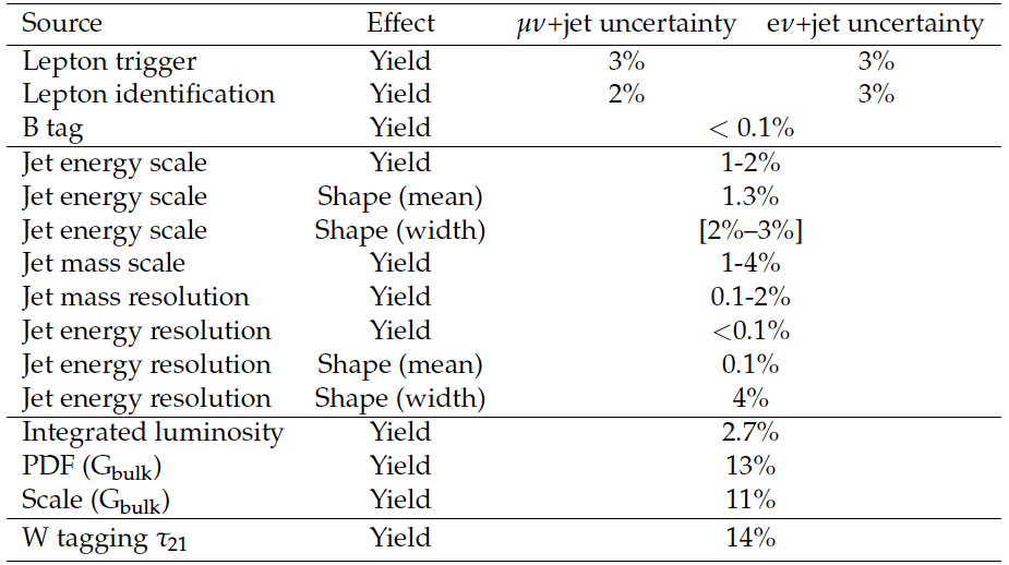
Table 1:
Summary of the systematic uncertainties and their impact on the signal yield and reconstructed $ {m_{\mathrm{WW} }} $ shape (mean and width) for both muon and electron channels. Ranges are denoted in square brackets. |
png pdf |
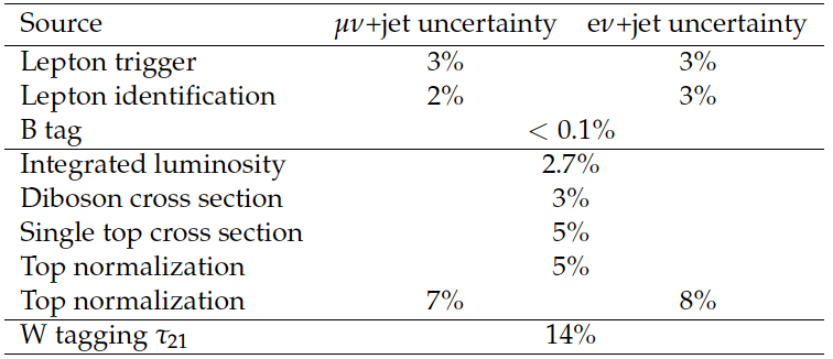
Table 2:
Systematic uncertainties affecting the background normalization. Ranges are denoted in square brackets. |
|
|
Compact Muon Solenoid LHC, CERN |
|

|

|

|

|

|