

Compact Muon Solenoid
LHC, CERN
| CMS-BPH-21-002 ; CERN-EP-2024-268 | ||
| Angular analysis of the $ {\mathrm{B}^0}\to\mathrm{ K^*(892)^0 }\mu^{+}\mu^{-} $ decay in proton-proton collisions at $ \sqrt{s}= $ 13 TeV | ||
| CMS Collaboration | ||
| 18 November 2024 | ||
| Phys. Lett. B 864 (2025) 139406 | ||
| Abstract: A full set of optimized observables is measured in an angular analysis of the decay $ {\mathrm{B}^0}\to\mathrm{ K^*(892)^0 }\mu^{+}\mu^{-} $ using a sample of proton-proton collisions at $ \sqrt{s}= $ 13 TeV, collected with the CMS detector at the LHC, corresponding to an integrated luminosity of 140 fb$ ^{-1} $. The analysis is performed in six bins of the squared invariant mass of the dimuon system, $ q^{2} $, over the range 1.1 $ < q^{2} < $ 16 GeV$^2 $. The results are among the most precise experimental measurements of the angular observables for this decay and are compared to a variety of predictions based on the standard model. Some of these predictions exhibit tension with the measurements. | ||
| Links: e-print arXiv:2411.11820 [hep-ex] (PDF) ; CDS record ; inSPIRE record ; HepData record ; Physics Briefing ; CADI line (restricted) ; | ||
| Figures & Tables | Summary | Additional Figures & Tables | References | CMS Publications |
|---|
| Figures | |

png pdf |
Figure 1:
Sketch representing the definition of the angles $ \theta_l $ (left), $ \theta_{\mathrm{K}} $ (center), and $ \phi $ (right). |

png pdf |
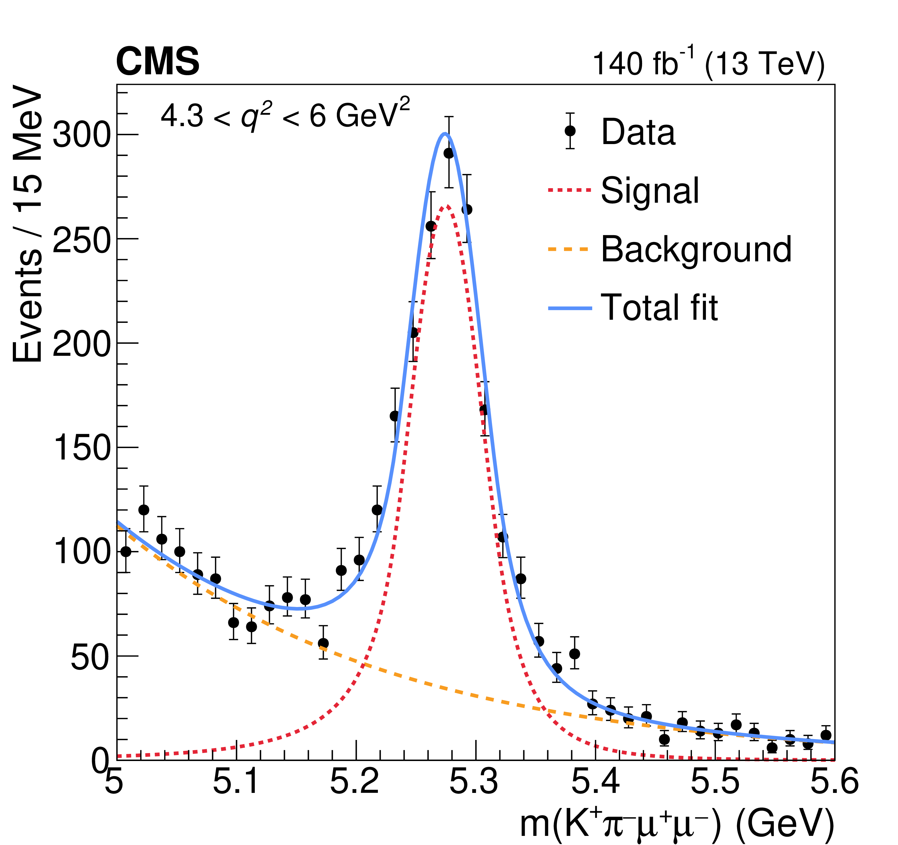
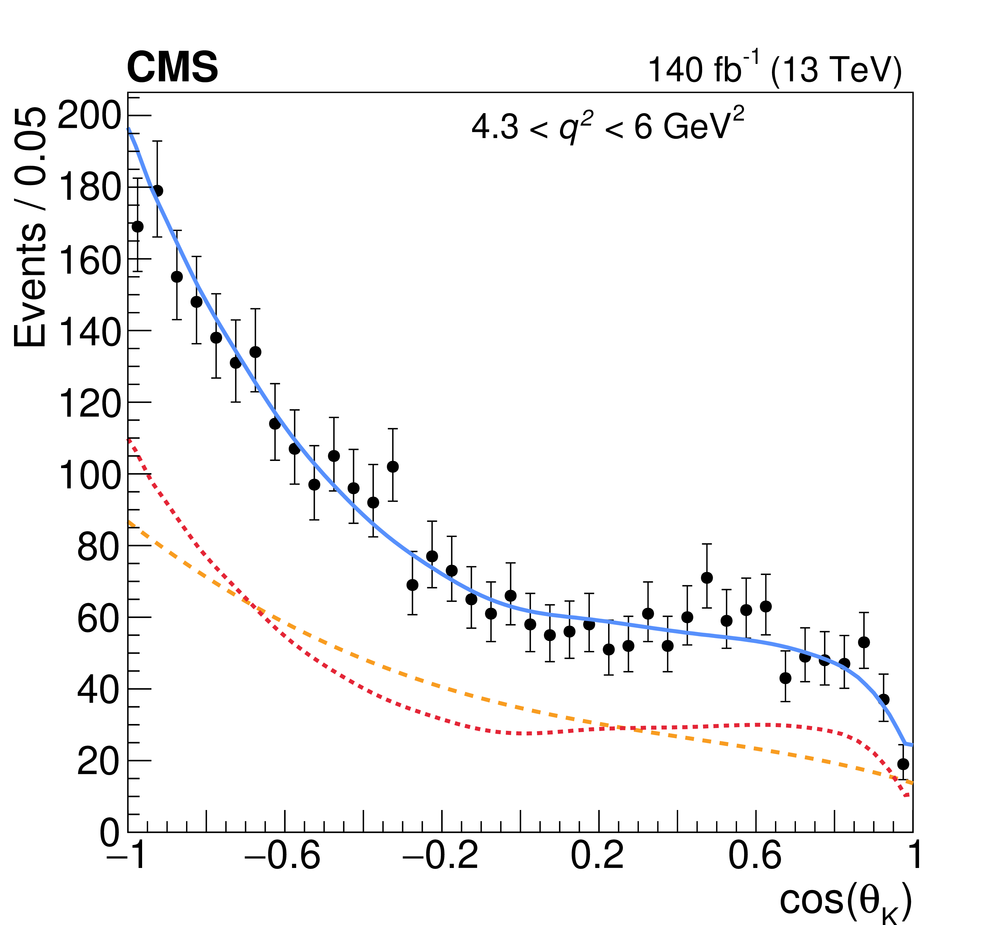
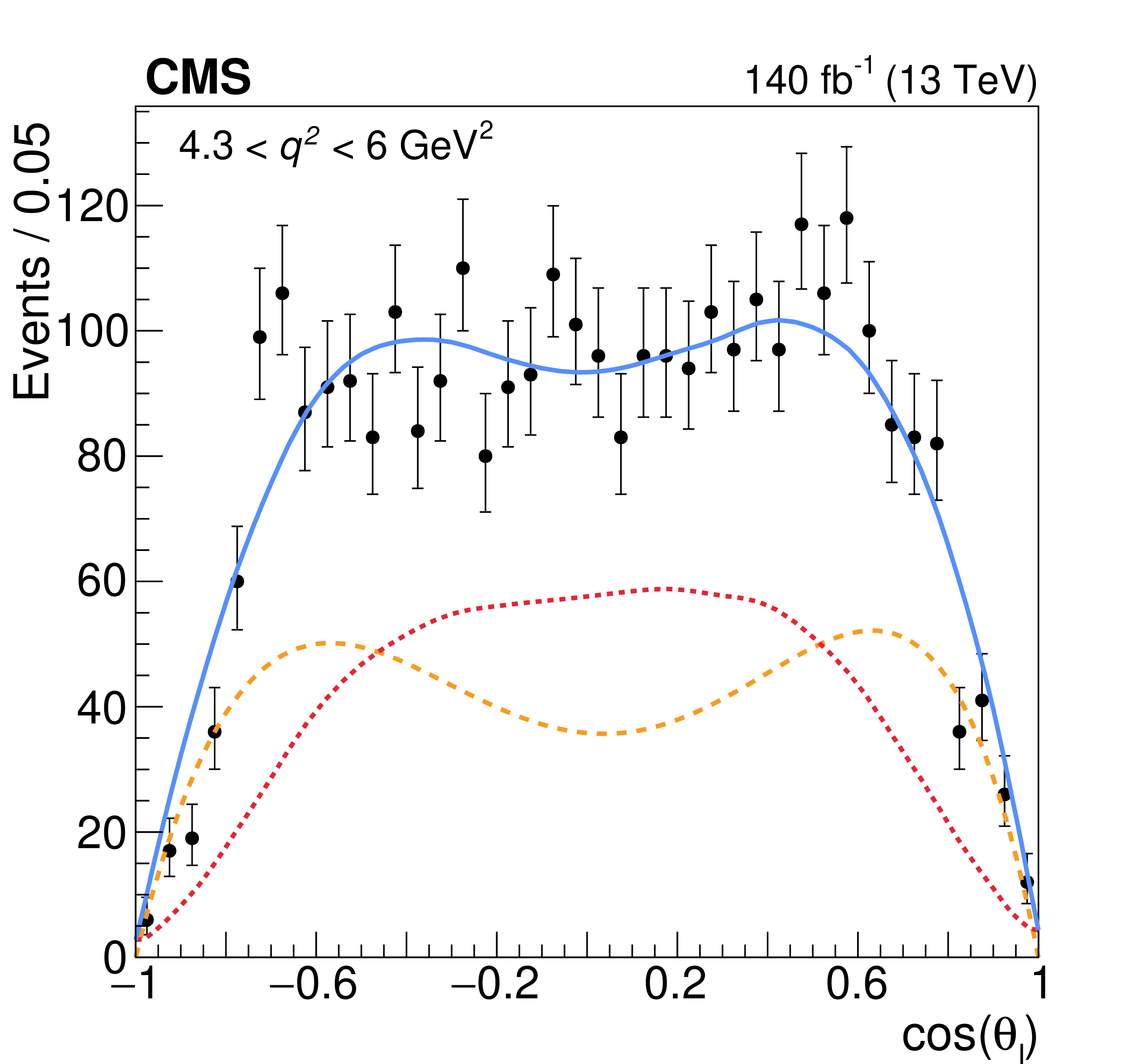
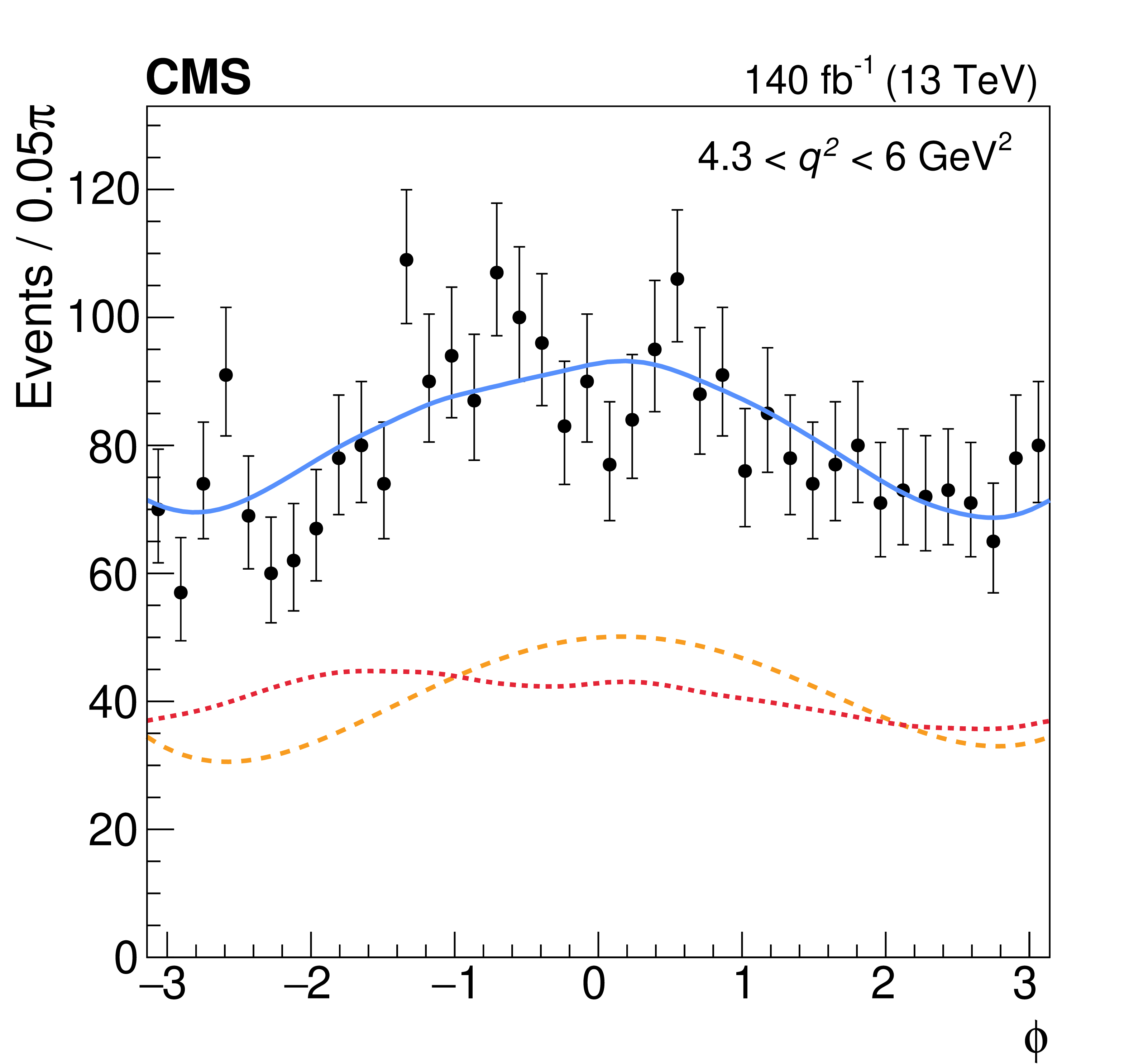
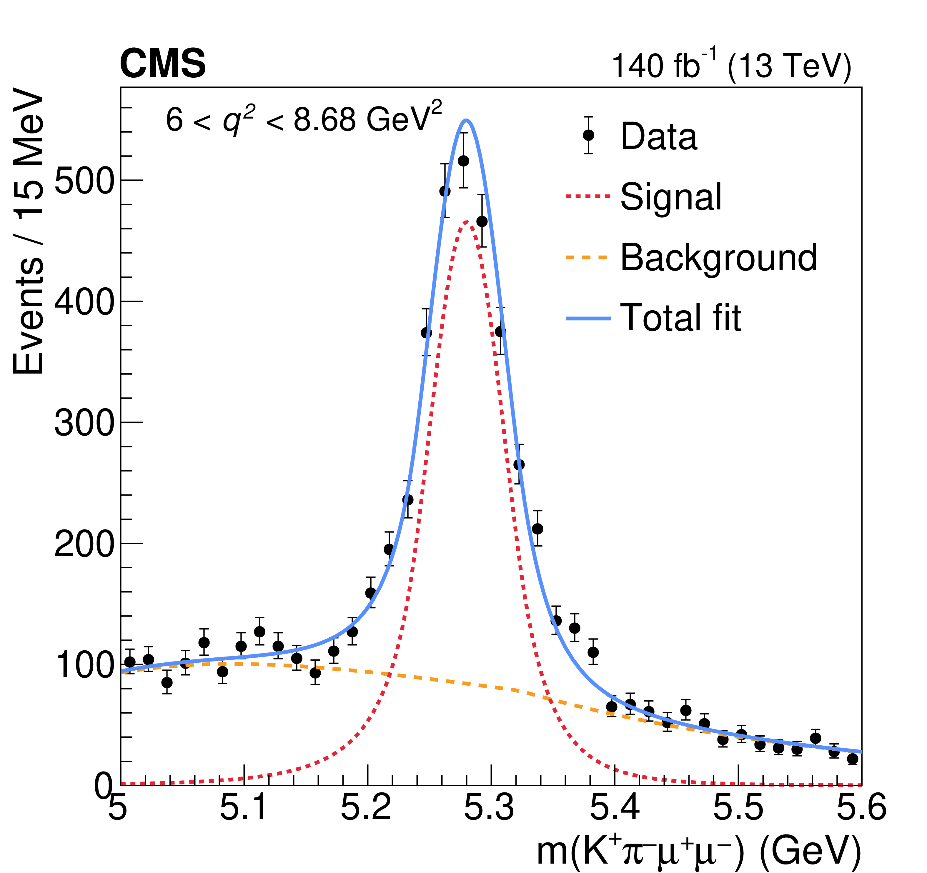
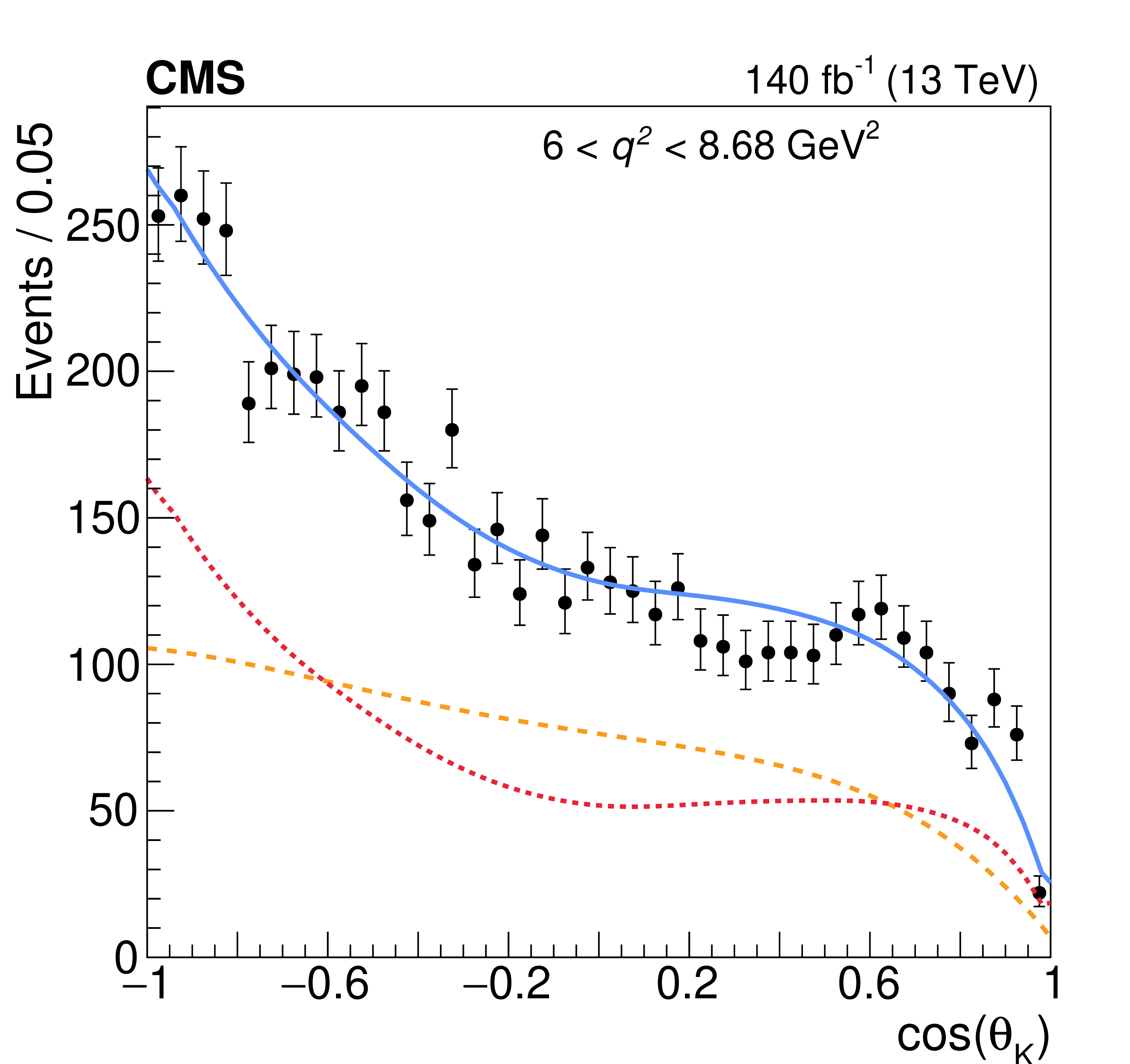
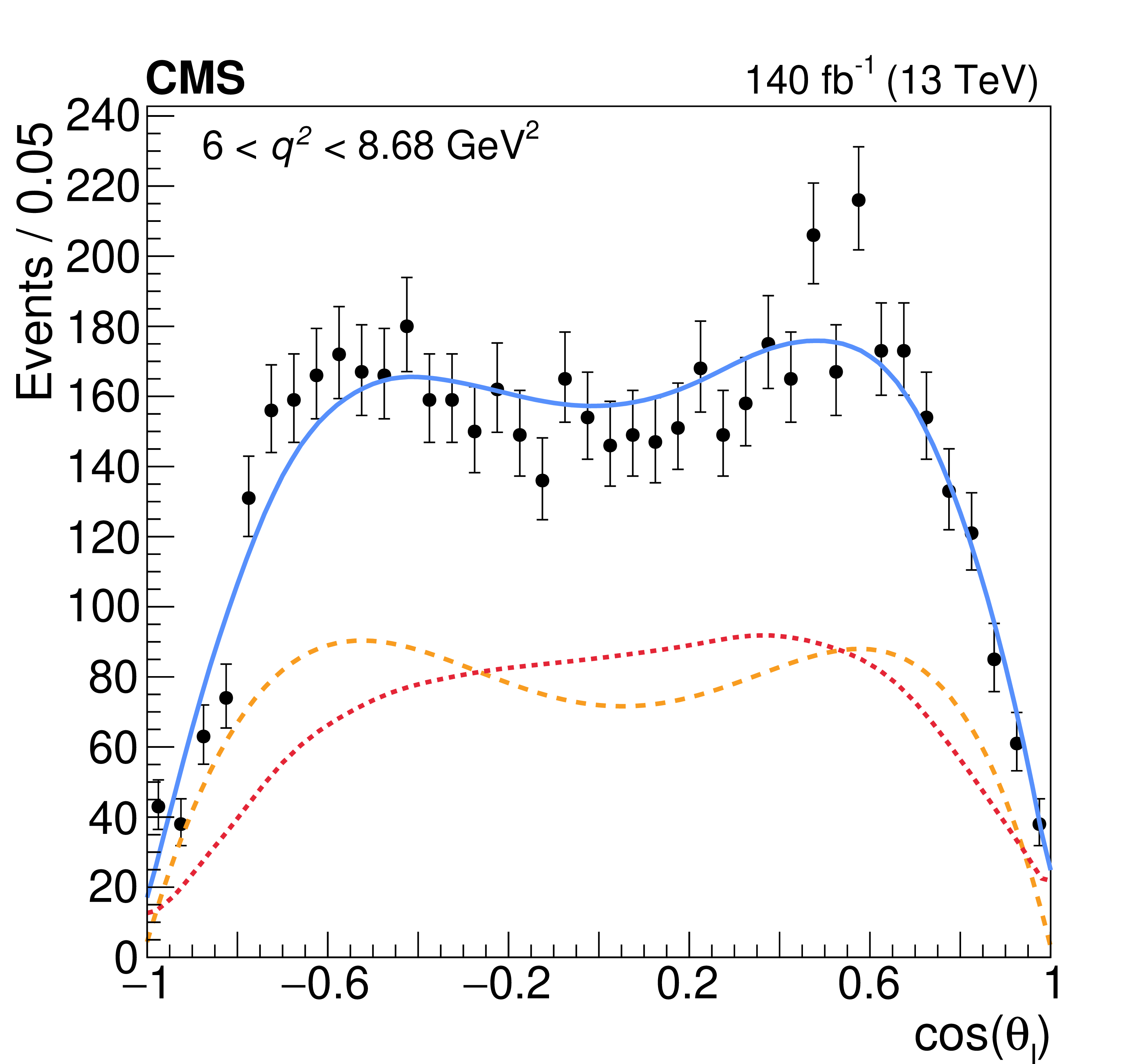
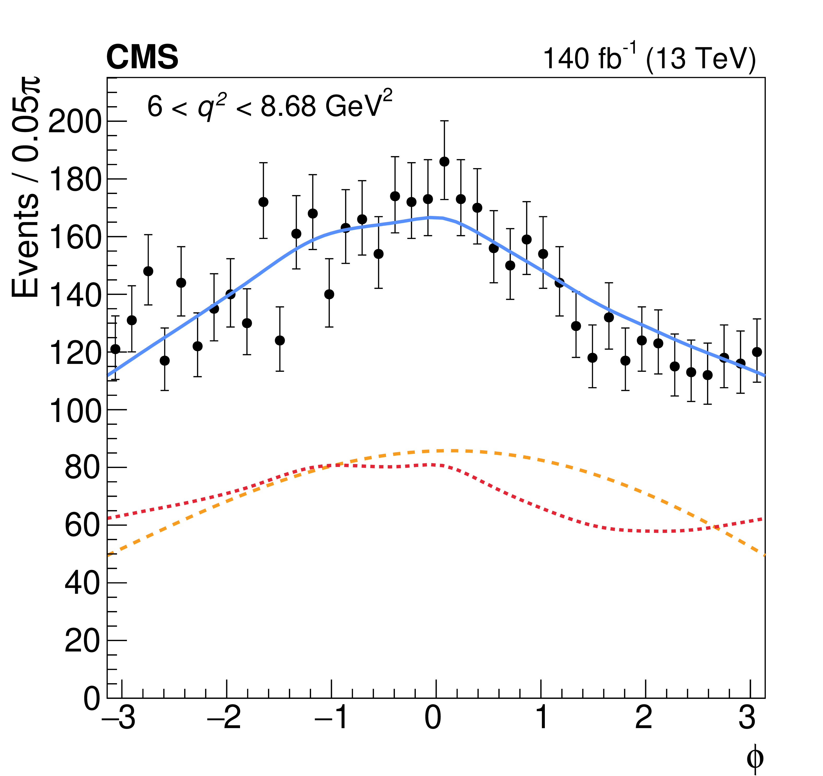
Figure 2:
Mass and angular distributions for the six $ q^{2} $ bins (one bin per row). The projections of the total fitted distribution (blue solid line) and its different components are overlaid. The signal is shown by the red dotted line, and the background by the orange dashed line. |

png pdf |
Figure 2-a:
Mass and angular distributions for the six $ q^{2} $ bins (one bin per row). The projections of the total fitted distribution (blue solid line) and its different components are overlaid. The signal is shown by the red dotted line, and the background by the orange dashed line. |

png pdf |
Figure 2-b:
Mass and angular distributions for the six $ q^{2} $ bins (one bin per row). The projections of the total fitted distribution (blue solid line) and its different components are overlaid. The signal is shown by the red dotted line, and the background by the orange dashed line. |

png pdf |
Figure 2-c:
Mass and angular distributions for the six $ q^{2} $ bins (one bin per row). The projections of the total fitted distribution (blue solid line) and its different components are overlaid. The signal is shown by the red dotted line, and the background by the orange dashed line. |

png pdf |
Figure 2-d:
Mass and angular distributions for the six $ q^{2} $ bins (one bin per row). The projections of the total fitted distribution (blue solid line) and its different components are overlaid. The signal is shown by the red dotted line, and the background by the orange dashed line. |

png pdf |
Figure 2-e:
Mass and angular distributions for the six $ q^{2} $ bins (one bin per row). The projections of the total fitted distribution (blue solid line) and its different components are overlaid. The signal is shown by the red dotted line, and the background by the orange dashed line. |

png pdf |
Figure 2-f:
Mass and angular distributions for the six $ q^{2} $ bins (one bin per row). The projections of the total fitted distribution (blue solid line) and its different components are overlaid. The signal is shown by the red dotted line, and the background by the orange dashed line. |

png pdf |
Figure 2-g:
Mass and angular distributions for the six $ q^{2} $ bins (one bin per row). The projections of the total fitted distribution (blue solid line) and its different components are overlaid. The signal is shown by the red dotted line, and the background by the orange dashed line. |

png pdf |
Figure 2-h:
Mass and angular distributions for the six $ q^{2} $ bins (one bin per row). The projections of the total fitted distribution (blue solid line) and its different components are overlaid. The signal is shown by the red dotted line, and the background by the orange dashed line. |
png pdf |
Figure 2-i:
Mass and angular distributions for the six $ q^{2} $ bins (one bin per row). The projections of the total fitted distribution (blue solid line) and its different components are overlaid. The signal is shown by the red dotted line, and the background by the orange dashed line. |
png pdf |
Figure 2-j:
Mass and angular distributions for the six $ q^{2} $ bins (one bin per row). The projections of the total fitted distribution (blue solid line) and its different components are overlaid. The signal is shown by the red dotted line, and the background by the orange dashed line. |
png pdf |
Figure 2-k:
Mass and angular distributions for the six $ q^{2} $ bins (one bin per row). The projections of the total fitted distribution (blue solid line) and its different components are overlaid. The signal is shown by the red dotted line, and the background by the orange dashed line. |
png pdf |
Figure 2-l:
Mass and angular distributions for the six $ q^{2} $ bins (one bin per row). The projections of the total fitted distribution (blue solid line) and its different components are overlaid. The signal is shown by the red dotted line, and the background by the orange dashed line. |
png pdf |
Figure 2-m:
Mass and angular distributions for the six $ q^{2} $ bins (one bin per row). The projections of the total fitted distribution (blue solid line) and its different components are overlaid. The signal is shown by the red dotted line, and the background by the orange dashed line. |
png pdf |
Figure 2-n:
Mass and angular distributions for the six $ q^{2} $ bins (one bin per row). The projections of the total fitted distribution (blue solid line) and its different components are overlaid. The signal is shown by the red dotted line, and the background by the orange dashed line. |
png pdf |
Figure 2-o:
Mass and angular distributions for the six $ q^{2} $ bins (one bin per row). The projections of the total fitted distribution (blue solid line) and its different components are overlaid. The signal is shown by the red dotted line, and the background by the orange dashed line. |
png pdf |
Figure 2-p:
Mass and angular distributions for the six $ q^{2} $ bins (one bin per row). The projections of the total fitted distribution (blue solid line) and its different components are overlaid. The signal is shown by the red dotted line, and the background by the orange dashed line. |
png pdf |
Figure 2-q:
Mass and angular distributions for the six $ q^{2} $ bins (one bin per row). The projections of the total fitted distribution (blue solid line) and its different components are overlaid. The signal is shown by the red dotted line, and the background by the orange dashed line. |
png pdf |
Figure 2-r:
Mass and angular distributions for the six $ q^{2} $ bins (one bin per row). The projections of the total fitted distribution (blue solid line) and its different components are overlaid. The signal is shown by the red dotted line, and the background by the orange dashed line. |
png pdf |
Figure 2-s:
Mass and angular distributions for the six $ q^{2} $ bins (one bin per row). The projections of the total fitted distribution (blue solid line) and its different components are overlaid. The signal is shown by the red dotted line, and the background by the orange dashed line. |
png pdf |
Figure 2-t:
Mass and angular distributions for the six $ q^{2} $ bins (one bin per row). The projections of the total fitted distribution (blue solid line) and its different components are overlaid. The signal is shown by the red dotted line, and the background by the orange dashed line. |
png pdf |
Figure 2-u:
Mass and angular distributions for the six $ q^{2} $ bins (one bin per row). The projections of the total fitted distribution (blue solid line) and its different components are overlaid. The signal is shown by the red dotted line, and the background by the orange dashed line. |
png pdf |
Figure 2-v:
Mass and angular distributions for the six $ q^{2} $ bins (one bin per row). The projections of the total fitted distribution (blue solid line) and its different components are overlaid. The signal is shown by the red dotted line, and the background by the orange dashed line. |
png pdf |
Figure 2-w:
Mass and angular distributions for the six $ q^{2} $ bins (one bin per row). The projections of the total fitted distribution (blue solid line) and its different components are overlaid. The signal is shown by the red dotted line, and the background by the orange dashed line. |
png pdf |
Figure 2-x:
Mass and angular distributions for the six $ q^{2} $ bins (one bin per row). The projections of the total fitted distribution (blue solid line) and its different components are overlaid. The signal is shown by the red dotted line, and the background by the orange dashed line. |

png pdf |
Figure 3:
Measurements of the angular observables versus $ q^{2} $. The inner vertical bars represent the statistical uncertainties, while the outer vertical bars give the total uncertainties. The horizontal bars show the bin widths. The vertical shaded regions correspond to the $ \mathrm{J}/\psi $ and $ \psi \text{(2S)} $ resonances. Predictions are shown, averaged in each bin, from Ref. [20] (labeled ABCDMN), and the EOS [50], flavio [51], and HEPfit [55] libraries. |

png pdf |
Figure 3-a:
Measurements of the angular observables versus $ q^{2} $. The inner vertical bars represent the statistical uncertainties, while the outer vertical bars give the total uncertainties. The horizontal bars show the bin widths. The vertical shaded regions correspond to the $ \mathrm{J}/\psi $ and $ \psi \text{(2S)} $ resonances. Predictions are shown, averaged in each bin, from Ref. [20] (labeled ABCDMN), and the EOS [50], flavio [51], and HEPfit [55] libraries. |

png pdf |
Figure 3-b:
Measurements of the angular observables versus $ q^{2} $. The inner vertical bars represent the statistical uncertainties, while the outer vertical bars give the total uncertainties. The horizontal bars show the bin widths. The vertical shaded regions correspond to the $ \mathrm{J}/\psi $ and $ \psi \text{(2S)} $ resonances. Predictions are shown, averaged in each bin, from Ref. [20] (labeled ABCDMN), and the EOS [50], flavio [51], and HEPfit [55] libraries. |

png pdf |
Figure 3-c:
Measurements of the angular observables versus $ q^{2} $. The inner vertical bars represent the statistical uncertainties, while the outer vertical bars give the total uncertainties. The horizontal bars show the bin widths. The vertical shaded regions correspond to the $ \mathrm{J}/\psi $ and $ \psi \text{(2S)} $ resonances. Predictions are shown, averaged in each bin, from Ref. [20] (labeled ABCDMN), and the EOS [50], flavio [51], and HEPfit [55] libraries. |

png pdf |
Figure 3-d:
Measurements of the angular observables versus $ q^{2} $. The inner vertical bars represent the statistical uncertainties, while the outer vertical bars give the total uncertainties. The horizontal bars show the bin widths. The vertical shaded regions correspond to the $ \mathrm{J}/\psi $ and $ \psi \text{(2S)} $ resonances. Predictions are shown, averaged in each bin, from Ref. [20] (labeled ABCDMN), and the EOS [50], flavio [51], and HEPfit [55] libraries. |

png pdf |
Figure 3-e:
Measurements of the angular observables versus $ q^{2} $. The inner vertical bars represent the statistical uncertainties, while the outer vertical bars give the total uncertainties. The horizontal bars show the bin widths. The vertical shaded regions correspond to the $ \mathrm{J}/\psi $ and $ \psi \text{(2S)} $ resonances. Predictions are shown, averaged in each bin, from Ref. [20] (labeled ABCDMN), and the EOS [50], flavio [51], and HEPfit [55] libraries. |

png pdf |
Figure 3-f:
Measurements of the angular observables versus $ q^{2} $. The inner vertical bars represent the statistical uncertainties, while the outer vertical bars give the total uncertainties. The horizontal bars show the bin widths. The vertical shaded regions correspond to the $ \mathrm{J}/\psi $ and $ \psi \text{(2S)} $ resonances. Predictions are shown, averaged in each bin, from Ref. [20] (labeled ABCDMN), and the EOS [50], flavio [51], and HEPfit [55] libraries. |

png pdf |
Figure 3-g:
Measurements of the angular observables versus $ q^{2} $. The inner vertical bars represent the statistical uncertainties, while the outer vertical bars give the total uncertainties. The horizontal bars show the bin widths. The vertical shaded regions correspond to the $ \mathrm{J}/\psi $ and $ \psi \text{(2S)} $ resonances. Predictions are shown, averaged in each bin, from Ref. [20] (labeled ABCDMN), and the EOS [50], flavio [51], and HEPfit [55] libraries. |

png pdf |
Figure 3-h:
Measurements of the angular observables versus $ q^{2} $. The inner vertical bars represent the statistical uncertainties, while the outer vertical bars give the total uncertainties. The horizontal bars show the bin widths. The vertical shaded regions correspond to the $ \mathrm{J}/\psi $ and $ \psi \text{(2S)} $ resonances. Predictions are shown, averaged in each bin, from Ref. [20] (labeled ABCDMN), and the EOS [50], flavio [51], and HEPfit [55] libraries. |

png pdf |
Figure 4:
Comparison of current measurements of $ P_2 $ and $ P^{\prime}_5 $ to a previous $ P_2 $ measurement by LHCb [16] and previous $ P^{\prime}_5 $ results from ATLAS [15], Belle [7], CMS [14], and LHCb [16]. The inner vertical bars represent the statistical uncertainties, while the outer vertical bars give the total uncertainties. The horizontal bars show the bin widths. |

png pdf |
Figure 4-a:
Comparison of current measurements of $ P_2 $ and $ P^{\prime}_5 $ to a previous $ P_2 $ measurement by LHCb [16] and previous $ P^{\prime}_5 $ results from ATLAS [15], Belle [7], CMS [14], and LHCb [16]. The inner vertical bars represent the statistical uncertainties, while the outer vertical bars give the total uncertainties. The horizontal bars show the bin widths. |

png pdf |
Figure 4-b:
Comparison of current measurements of $ P_2 $ and $ P^{\prime}_5 $ to a previous $ P_2 $ measurement by LHCb [16] and previous $ P^{\prime}_5 $ results from ATLAS [15], Belle [7], CMS [14], and LHCb [16]. The inner vertical bars represent the statistical uncertainties, while the outer vertical bars give the total uncertainties. The horizontal bars show the bin widths. |
| Tables | |

png pdf |
Table 1:
The uncertainties considered in the analysis on the various angular observables. For each source of uncertainty, the range covers the absolute variation observed across the $ q^{2} $ bins. |

png pdf |
Table 2:
The measured CP-averaged angular observables, in the corresponding $ q^{2} $ bins. The first uncertainty is statistical and the second is systematic. |
| Summary |
| In summary, the study of the full angular distribution of the flavor-changing neutral-current $ {\mathrm{B}^0}\to \mathrm{ K^{*0} }\mu^{+}\mu^{-} $ decay has been performed using 140 fb$ ^{-1} $ of proton-proton collision data recorded by the CMS detector at the LHC at $ \sqrt{s}= $ 13 TeV. A complete set of observables has been measured via unbinned maximum likelihood fits to the $ {\mathrm{B}^0} $ candidate mass and angular variables, in bins of the squared invariant mass of the dimuon system ranging from 1.1 to 16 GeV$^2$. The measurements are compared to a variety of predictions based on the standard model, with tension in a few of the angular observables seen for some of the predictions, as is also reported by other experiments. These results are among the most precise experimental measurements of the angular observables of this decay, and provide a valuable contribution to the understanding of the $ \mathrm{b}\to\mathrm{s}\ell^{+}\ell^{-} $ processes. |
| Additional Figures | |

png pdf |
Additional Figure 1:
Mass and angular distributions for 1.1 $ < q^{2} < $ 2 GeV$^{2}$. The projections of the total fitted distribution (in blue) and its different components are overlaid. The signal is shown by the red dotted line, and the background by the orange dashed line. |

png pdf |
Additional Figure 1-a:
Mass and angular distributions for 1.1 $ < q^{2} < $ 2 GeV$^{2}$. The projections of the total fitted distribution (in blue) and its different components are overlaid. The signal is shown by the red dotted line, and the background by the orange dashed line. |

png pdf |
Additional Figure 1-b:
Mass and angular distributions for 1.1 $ < q^{2} < $ 2 GeV$^{2}$. The projections of the total fitted distribution (in blue) and its different components are overlaid. The signal is shown by the red dotted line, and the background by the orange dashed line. |

png pdf |
Additional Figure 1-c:
Mass and angular distributions for 1.1 $ < q^{2} < $ 2 GeV$^{2}$. The projections of the total fitted distribution (in blue) and its different components are overlaid. The signal is shown by the red dotted line, and the background by the orange dashed line. |

png pdf |
Additional Figure 1-d:
Mass and angular distributions for 1.1 $ < q^{2} < $ 2 GeV$^{2}$. The projections of the total fitted distribution (in blue) and its different components are overlaid. The signal is shown by the red dotted line, and the background by the orange dashed line. |

png pdf |
Additional Figure 2:
Mass and angular distributions for 6 $ < q^{2} < $ 8.68 GeV$^{2}$. The projections of the total fitted distribution (in blue) and its different components are overlaid. The signal is shown by the red dotted line, and the background by the orange dashed line. |

png pdf |
Additional Figure 2-a:
Mass and angular distributions for 6 $ < q^{2} < $ 8.68 GeV$^{2}$. The projections of the total fitted distribution (in blue) and its different components are overlaid. The signal is shown by the red dotted line, and the background by the orange dashed line. |

png pdf |
Additional Figure 2-b:
Mass and angular distributions for 6 $ < q^{2} < $ 8.68 GeV$^{2}$. The projections of the total fitted distribution (in blue) and its different components are overlaid. The signal is shown by the red dotted line, and the background by the orange dashed line. |

png pdf |
Additional Figure 2-c:
Mass and angular distributions for 6 $ < q^{2} < $ 8.68 GeV$^{2}$. The projections of the total fitted distribution (in blue) and its different components are overlaid. The signal is shown by the red dotted line, and the background by the orange dashed line. |

png pdf |
Additional Figure 2-d:
Mass and angular distributions for 6 $ < q^{2} < $ 8.68 GeV$^{2}$. The projections of the total fitted distribution (in blue) and its different components are overlaid. The signal is shown by the red dotted line, and the background by the orange dashed line. |

png pdf |
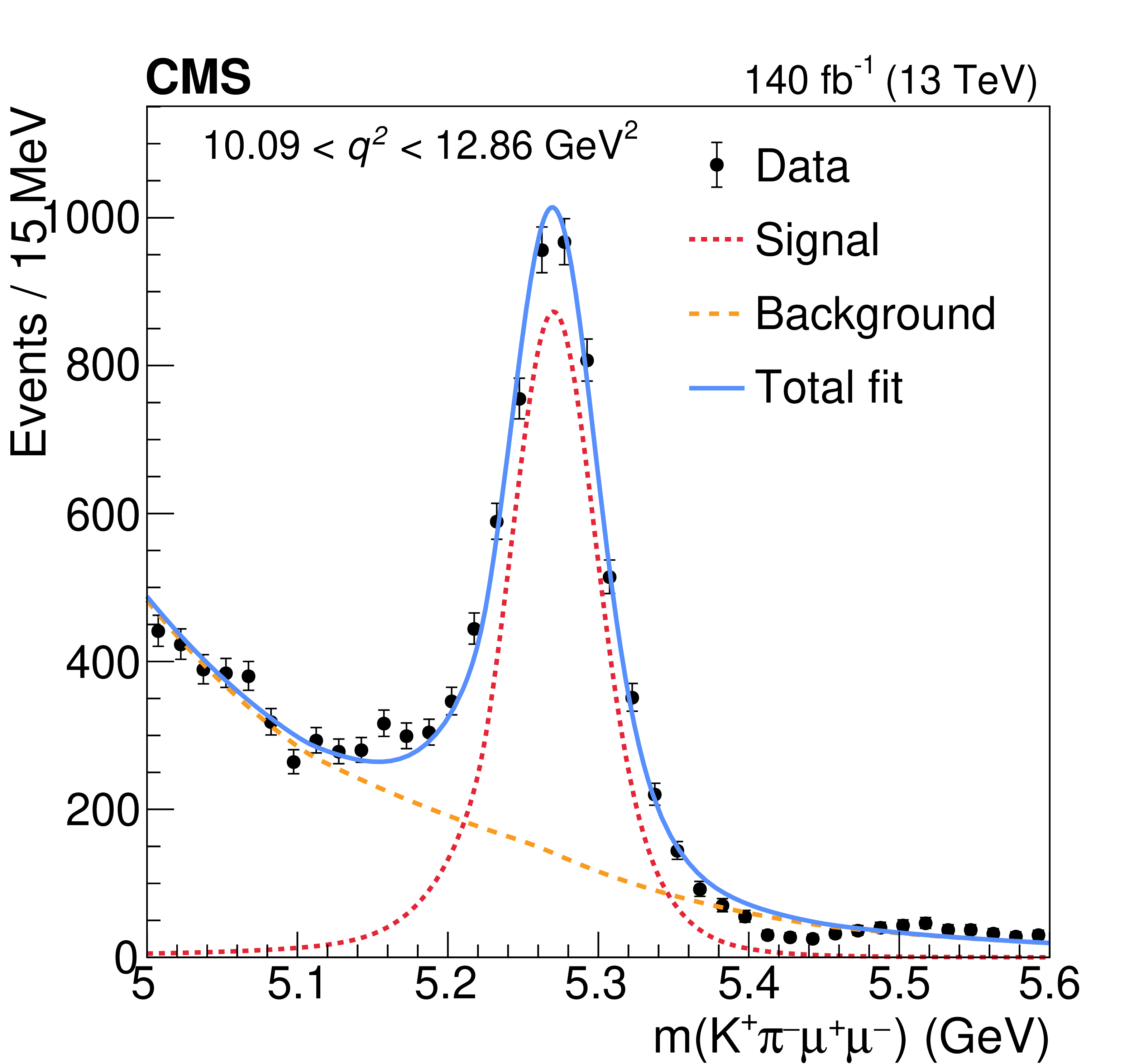
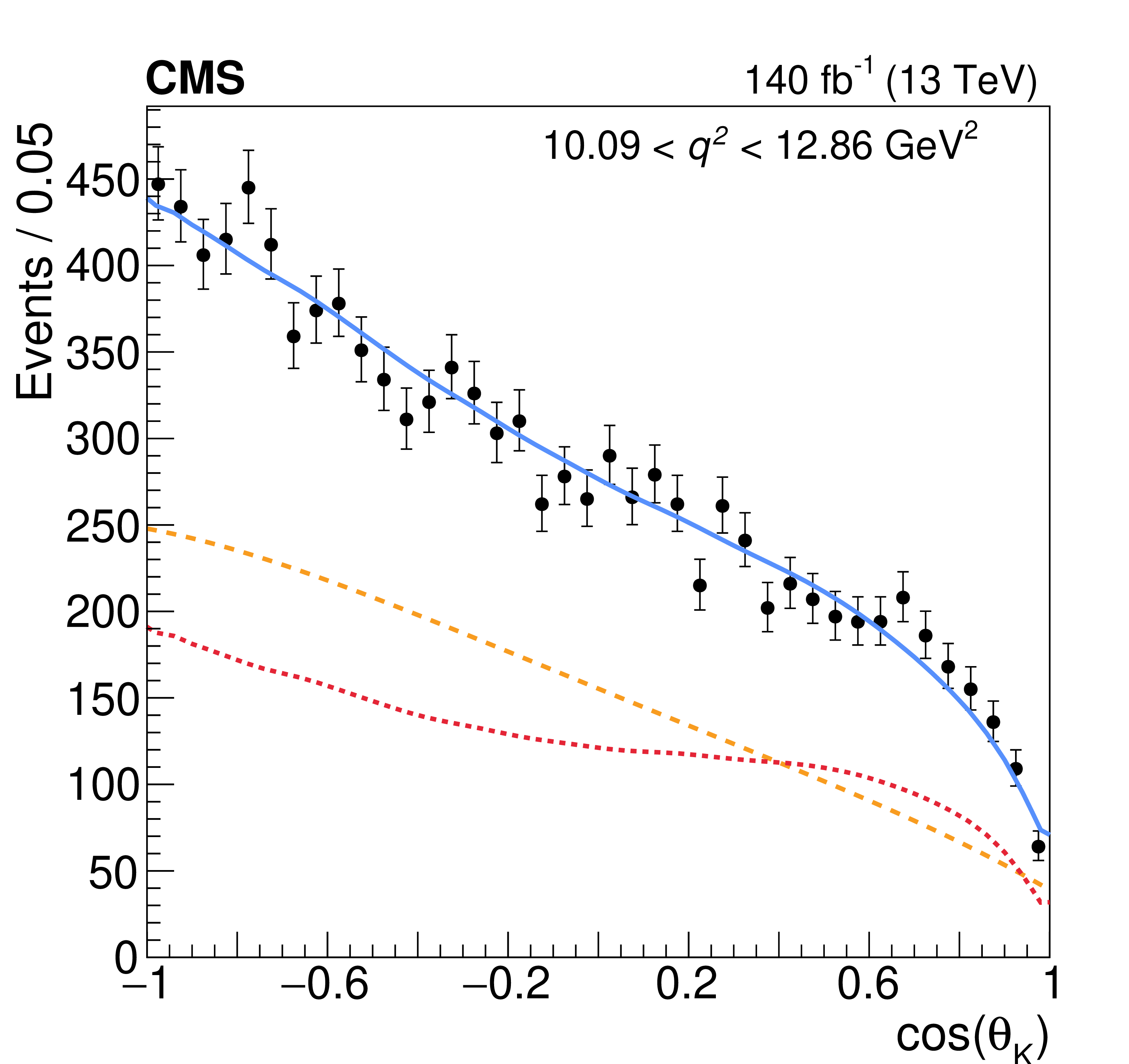
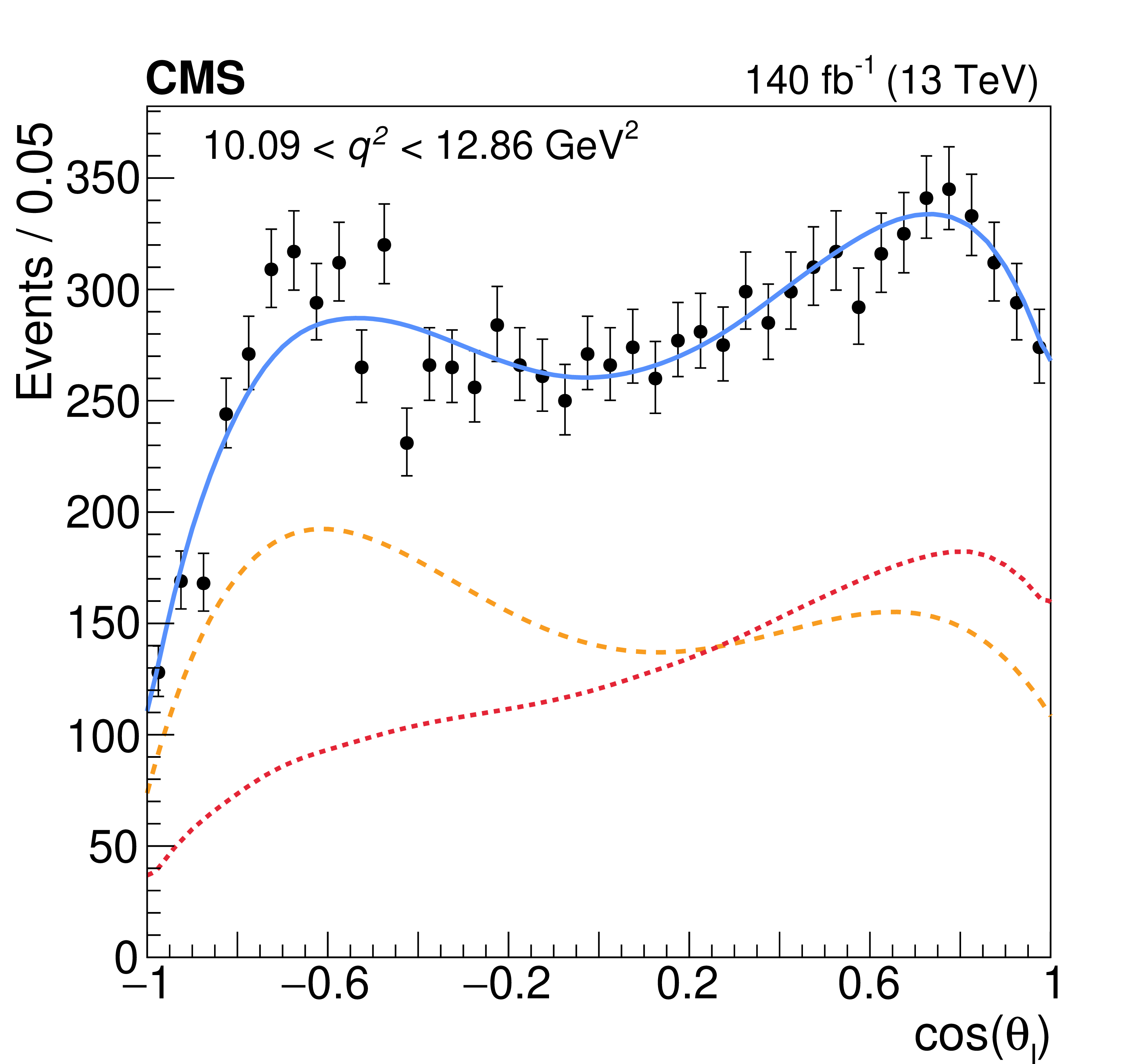
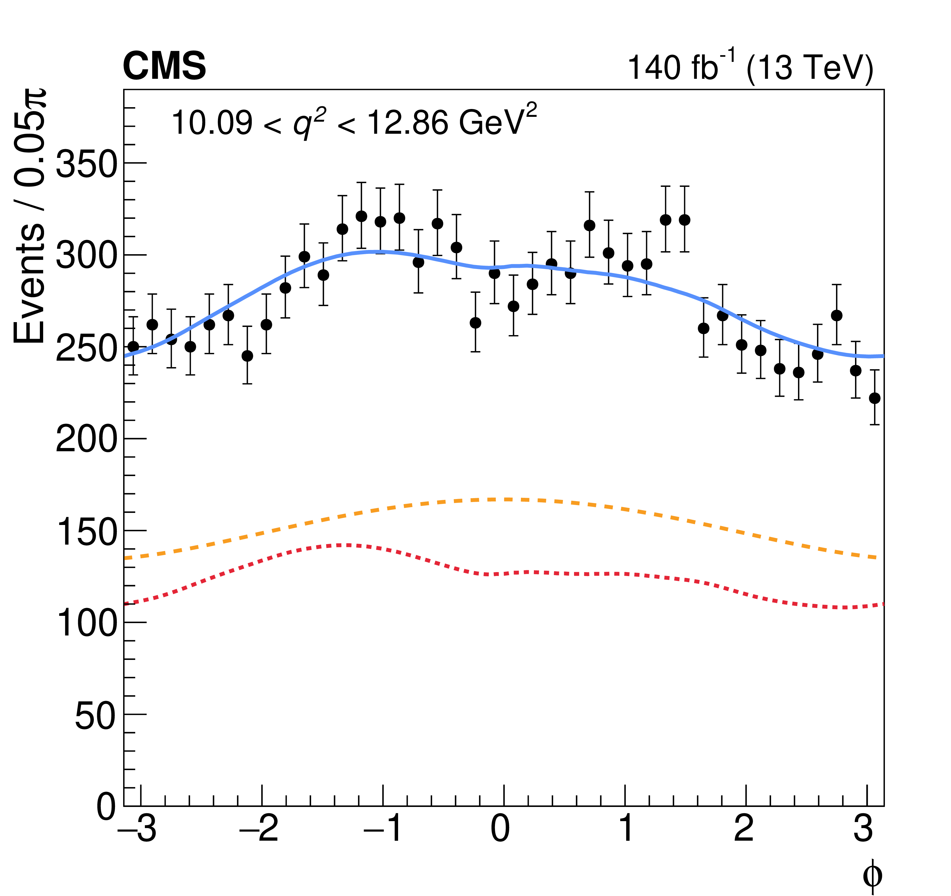
Additional Figure 3:
Mass and angular distributions for 10.09 $ < q^{2} < $ 12.86 GeV$^{2}$. The projections of the total fitted distribution (in blue) and its different components are overlaid. The signal is shown by the red dotted line, and the background by the orange dashed line. |

png pdf |
Additional Figure 3-a:
Mass and angular distributions for 10.09 $ < q^{2} < $ 12.86 GeV$^{2}$. The projections of the total fitted distribution (in blue) and its different components are overlaid. The signal is shown by the red dotted line, and the background by the orange dashed line. |

png pdf |
Additional Figure 3-b:
Mass and angular distributions for 10.09 $ < q^{2} < $ 12.86 GeV$^{2}$. The projections of the total fitted distribution (in blue) and its different components are overlaid. The signal is shown by the red dotted line, and the background by the orange dashed line. |

png pdf |
Additional Figure 3-c:
Mass and angular distributions for 10.09 $ < q^{2} < $ 12.86 GeV$^{2}$. The projections of the total fitted distribution (in blue) and its different components are overlaid. The signal is shown by the red dotted line, and the background by the orange dashed line. |

png pdf |
Additional Figure 3-d:
Mass and angular distributions for 10.09 $ < q^{2} < $ 12.86 GeV$^{2}$. The projections of the total fitted distribution (in blue) and its different components are overlaid. The signal is shown by the red dotted line, and the background by the orange dashed line. |

png pdf |
Additional Figure 4:
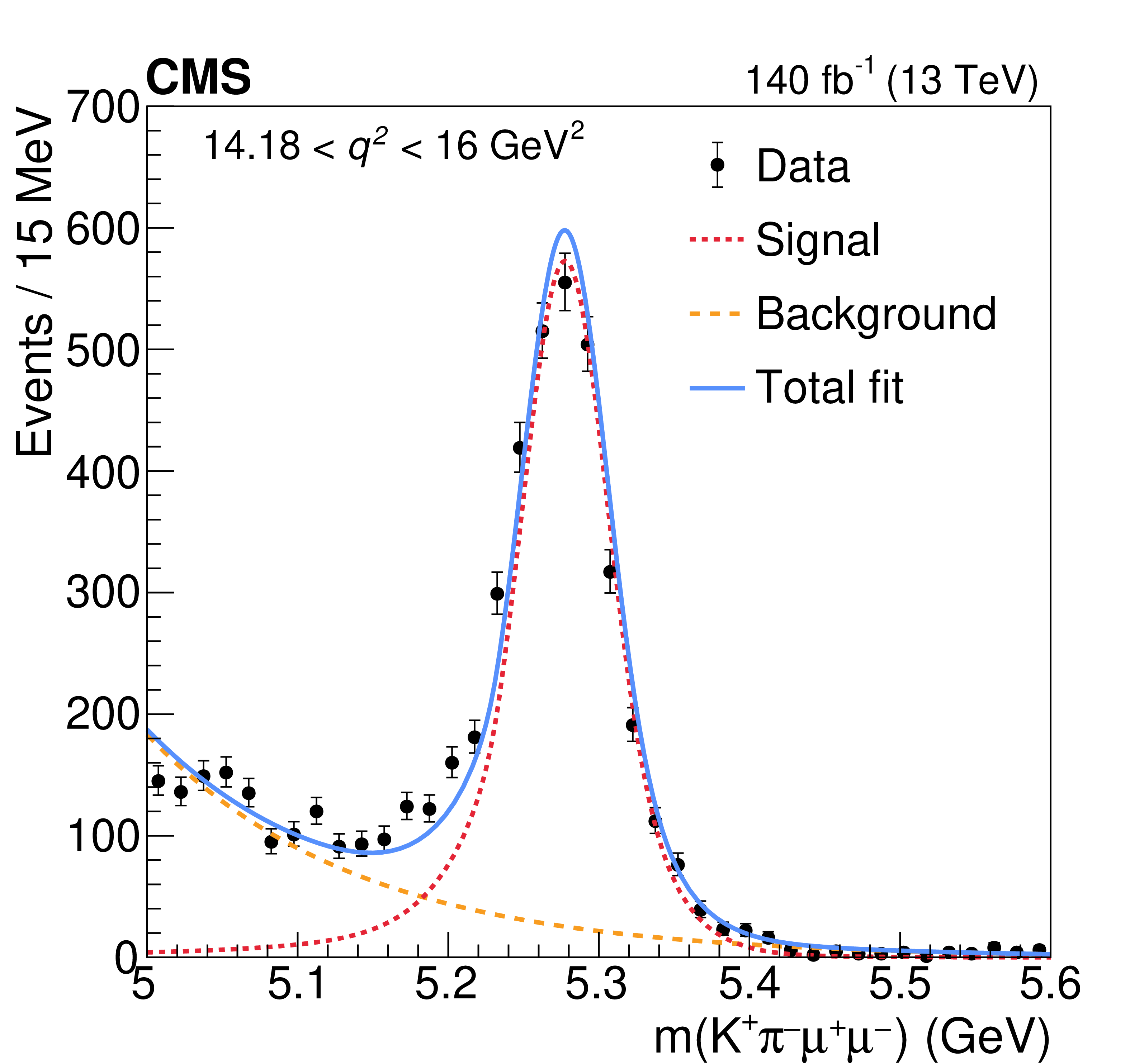
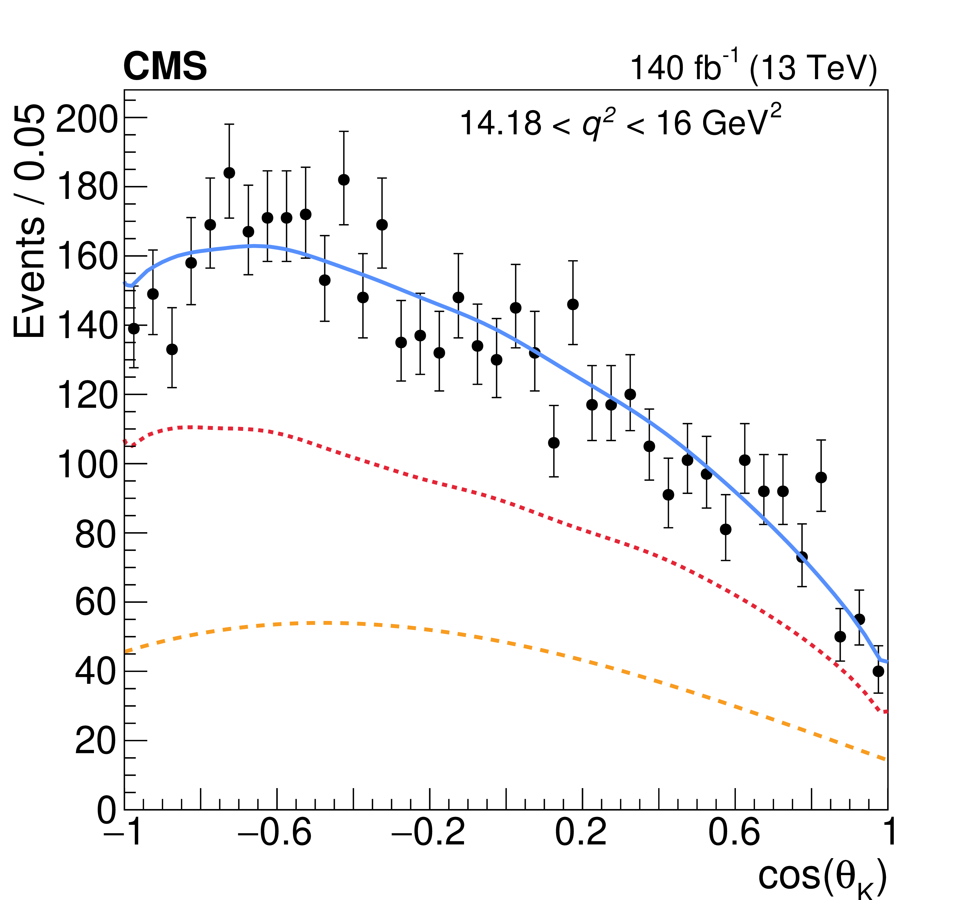
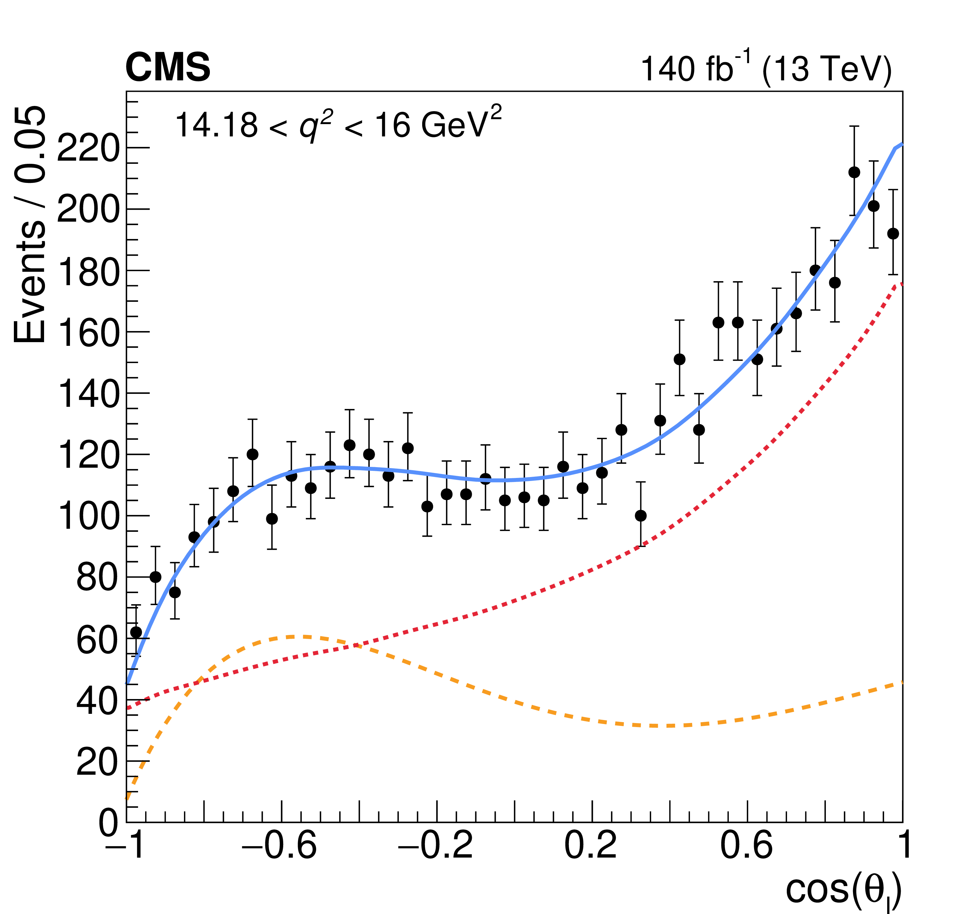
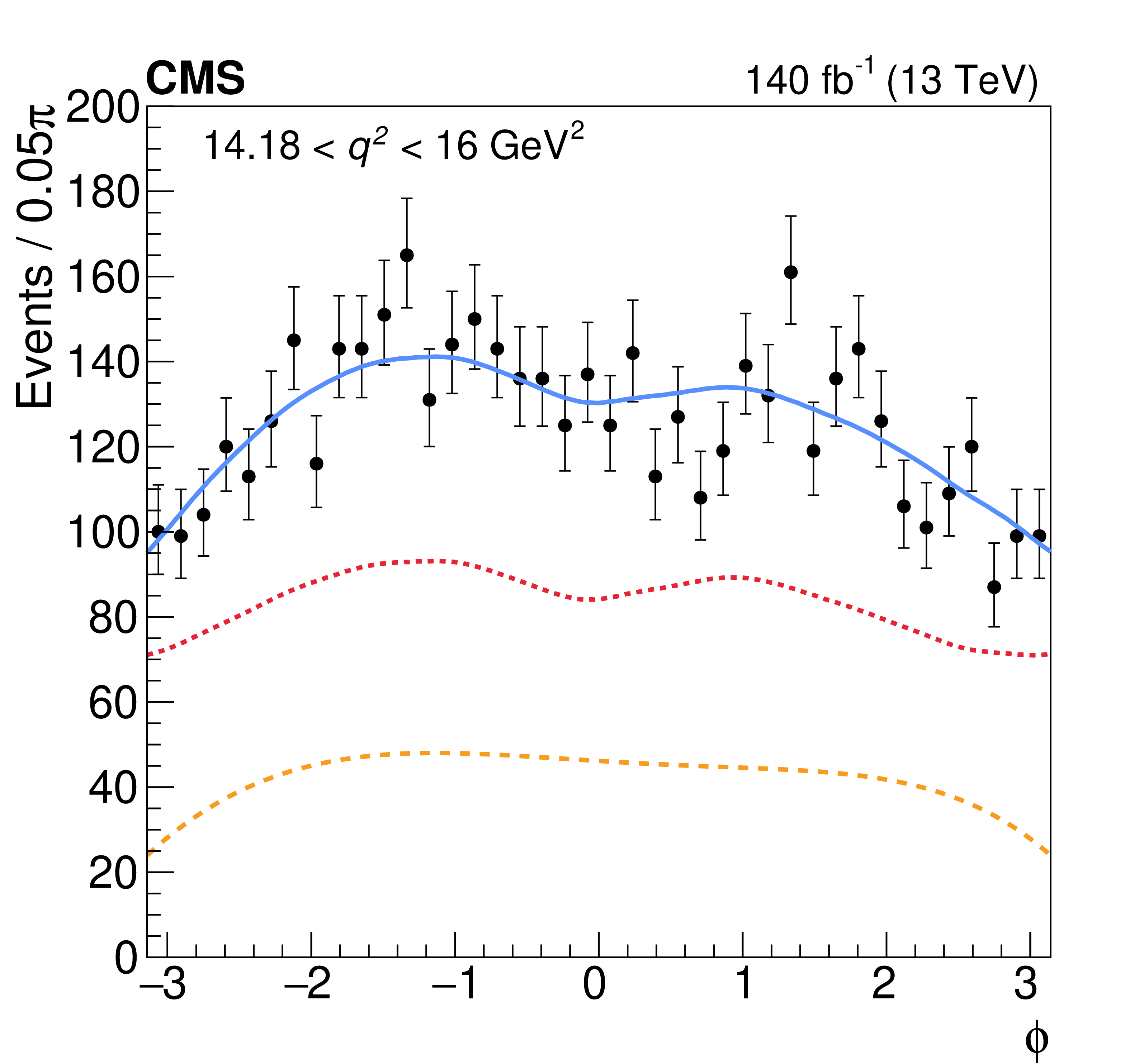
Mass and angular distributions for 14.18 $ < q^{2} < $ 16 GeV$^{2}$. The projections of the total fitted distribution (in blue) and its different components are overlaid. The signal is shown by the red dotted line, and the background by the orange dashed line. |

png pdf |
Additional Figure 4-a:
Mass and angular distributions for 14.18 $ < q^{2} < $ 16 GeV$^{2}$. The projections of the total fitted distribution (in blue) and its different components are overlaid. The signal is shown by the red dotted line, and the background by the orange dashed line. |

png pdf |
Additional Figure 4-b:
Mass and angular distributions for 14.18 $ < q^{2} < $ 16 GeV$^{2}$. The projections of the total fitted distribution (in blue) and its different components are overlaid. The signal is shown by the red dotted line, and the background by the orange dashed line. |

png pdf |
Additional Figure 4-c:
Mass and angular distributions for 14.18 $ < q^{2} < $ 16 GeV$^{2}$. The projections of the total fitted distribution (in blue) and its different components are overlaid. The signal is shown by the red dotted line, and the background by the orange dashed line. |

png pdf |
Additional Figure 4-d:
Mass and angular distributions for 14.18 $ < q^{2} < $ 16 GeV$^{2}$. The projections of the total fitted distribution (in blue) and its different components are overlaid. The signal is shown by the red dotted line, and the background by the orange dashed line. |

png pdf |
Additional Figure 5:
Comparison of current measurements of $ F_\mathrm{L} $ to previous results from ATLAS [15], CMS [13], and LHCb [16]. The inner vertical bars represent the statistical uncertainties, while the outer vertical bars give the total uncertainties. The horizontal bars show the bin widths. |

png pdf |
Additional Figure 6:
Comparison of current measurements of $ P_1 $ to previous results from ATLAS [15], CMS [14], and LHCb [16]. The inner vertical bars represent the statistical uncertainties, while the outer vertical bars give the total uncertainties. The horizontal bars show the bin widths. |

png pdf |
Additional Figure 7:
Comparison of current measurements of $ P_3 $ to previous results from LHCb [16]. The inner vertical bars represent the statistical uncertainties, while the outer vertical bars give the total uncertainties. The horizontal bars show the bin widths. |

png pdf |
Additional Figure 8:
Comparison of current measurements of $ P_4^{\prime} $ to previous results from ATLAS [15], Belle [7], and LHCb [16]. The inner vertical bars represent the statistical uncertainties, while the outer vertical bars give the total uncertainties. The horizontal bars show the bin widths. The definition of the $ P_4^{\prime} $ observable is the one presented in Ref. [24]: the results from ATLAS, Belle, and LHCb Collaborations are therefore scaled by a factor of two to superimpose them on the same plot. |

png pdf |
Additional Figure 9:
Comparison of current measurements of $ P_6^{\prime} $ to previous results from ATLAS [15] and LHCb [16]. The inner vertical bars represent the statistical uncertainties, while the outer vertical bars give the total uncertainties. The horizontal bars show the bin widths. The definition of the $ P_6^{\prime} $ observable is the one presented in Ref. [24]: the results from the LHCb Collaboration are therefore scaled by a factor of minus one to superimpose them on the same plot. |

png pdf |
Additional Figure 10:
Comparison of current measurements of $ P_8^{\prime} $ to previous results from ATLAS [15] and LHCb [16]. The inner vertical bars represent the statistical uncertainties, while the outer vertical bars give the total uncertainties. The horizontal bars show the bin widths. The definition of the $ P_8^{\prime} $ observable is the one presented in Ref. [24]: the results from LHCb and ATLAS Collaborations are therefore scaled by a factor of two to superimpose them on the same plot. |

png pdf |
Additional Figure 11:
The various sources of systematic uncertainty per each $ q^{2} $ bin, for the $ F_\mathrm{L} $ observable. In all cases where the statistical uncertainty is asymmetric, the maximum of the two uncertainties is represented. The total systematic uncertainty and the statistical uncertainty are shown by the dotted area and white bar, respectively. |

png pdf |
Additional Figure 12:
The various sources of systematic uncertainty per each $ q^{2} $ bin, for the $ P_1 $ observable. In all cases where the statistical uncertainty is asymmetric, the maximum of the two uncertainties is represented. The total systematic uncertainty and the statistical uncertainty are shown by the dotted area and white bar, respectively. |

png pdf |
Additional Figure 13:
The various sources of systematic uncertainty per each $ q^{2} $ bin, for the $ P_2 $ observable. In all cases where the statistical uncertainty is asymmetric, the maximum of the two uncertainties is represented. The total systematic uncertainty and the statistical uncertainty are shown by the dotted area and white bar, respectively. |

png pdf |
Additional Figure 14:
The various sources of systematic uncertainty per each $ q^{2} $ bin, for the $ P_3 $ observable. In all cases where the statistical uncertainty is asymmetric, the maximum of the two uncertainties is represented. The total systematic uncertainty and the statistical uncertainty are shown by the dotted area and white bar, respectively. |

png pdf |
Additional Figure 15:
The various sources of systematic uncertainty per each $ q^{2} $ bin, for the $ P_4^{\prime} $ observable. In all cases where the statistical uncertainty is asymmetric, the maximum of the two uncertainties is represented. The total systematic uncertainty and the statistical uncertainty are shown by the dotted area and white bar, respectively. |

png pdf |
Additional Figure 16:
The various sources of systematic uncertainty per each $ q^{2} $ bin, for the $ P_5^{\prime} $ observable. In all cases where the statistical uncertainty is asymmetric, the maximum of the two uncertainties is represented. The total systematic uncertainty and the statistical uncertainty are shown by the dotted area and white bar, respectively. |

png pdf |
Additional Figure 17:
The various sources of systematic uncertainty per each $ q^{2} $ bin, for the $ P_6^{\prime} $ observable. In all cases where the statistical uncertainty is asymmetric, the maximum of the two uncertainties is represented. The total systematic uncertainty and the statistical uncertainty are shown by the dotted area and white bar, respectively. |

png pdf |
Additional Figure 18:
The various sources of systematic uncertainty per each $ q^{2} $ bin, for the $ P_8^{\prime} $ observable. In all cases where the statistical uncertainty is asymmetric, the maximum of the two uncertainties is represented. The total systematic uncertainty and the statistical uncertainty are shown by the dotted area and white bar, respectively. |

png pdf |
Additional Figure 19:
Projections on the angular variables of the three-dimensional efficiency functions for signal candidates with correct (blue line) and wrong (orange line) flavor assignment, for 1.1 $ < q^{2} < $ 2 GeV$^{2}$. These functions represent the combination of detector acceptance and efficiency for signal candidates, calculated on a sample of simulated $ {\mathrm{B}^0} $ mesons with $ |\eta| < $ 3, with conditions corresponding to the data collected in 2018. |

png pdf |
Additional Figure 19-a:
Projections on the angular variables of the three-dimensional efficiency functions for signal candidates with correct (blue line) and wrong (orange line) flavor assignment, for 1.1 $ < q^{2} < $ 2 GeV$^{2}$. These functions represent the combination of detector acceptance and efficiency for signal candidates, calculated on a sample of simulated $ {\mathrm{B}^0} $ mesons with $ |\eta| < $ 3, with conditions corresponding to the data collected in 2018. |

png pdf |
Additional Figure 19-b:
Projections on the angular variables of the three-dimensional efficiency functions for signal candidates with correct (blue line) and wrong (orange line) flavor assignment, for 1.1 $ < q^{2} < $ 2 GeV$^{2}$. These functions represent the combination of detector acceptance and efficiency for signal candidates, calculated on a sample of simulated $ {\mathrm{B}^0} $ mesons with $ |\eta| < $ 3, with conditions corresponding to the data collected in 2018. |

png pdf |
Additional Figure 19-c:
Projections on the angular variables of the three-dimensional efficiency functions for signal candidates with correct (blue line) and wrong (orange line) flavor assignment, for 1.1 $ < q^{2} < $ 2 GeV$^{2}$. These functions represent the combination of detector acceptance and efficiency for signal candidates, calculated on a sample of simulated $ {\mathrm{B}^0} $ mesons with $ |\eta| < $ 3, with conditions corresponding to the data collected in 2018. |

png pdf |
Additional Figure 20:
Projections on the angular variables of the three-dimensional efficiency functions for signal candidates with correct (blue line) and wrong (orange line) flavor assignment, for 2 $ < q^{2} < $ 4.3 GeV$^{2}$. These functions represent the combination of detector acceptance and efficiency for signal candidates, calculated on a sample of simulated $ {\mathrm{B}^0} $ mesons with $ |\eta| < $ 3, with conditions corresponding to the data collected in 2018. |

png pdf |
Additional Figure 20-a:
Projections on the angular variables of the three-dimensional efficiency functions for signal candidates with correct (blue line) and wrong (orange line) flavor assignment, for 2 $ < q^{2} < $ 4.3 GeV$^{2}$. These functions represent the combination of detector acceptance and efficiency for signal candidates, calculated on a sample of simulated $ {\mathrm{B}^0} $ mesons with $ |\eta| < $ 3, with conditions corresponding to the data collected in 2018. |

png pdf |
Additional Figure 20-b:
Projections on the angular variables of the three-dimensional efficiency functions for signal candidates with correct (blue line) and wrong (orange line) flavor assignment, for 2 $ < q^{2} < $ 4.3 GeV$^{2}$. These functions represent the combination of detector acceptance and efficiency for signal candidates, calculated on a sample of simulated $ {\mathrm{B}^0} $ mesons with $ |\eta| < $ 3, with conditions corresponding to the data collected in 2018. |

png pdf |
Additional Figure 20-c:
Projections on the angular variables of the three-dimensional efficiency functions for signal candidates with correct (blue line) and wrong (orange line) flavor assignment, for 2 $ < q^{2} < $ 4.3 GeV$^{2}$. These functions represent the combination of detector acceptance and efficiency for signal candidates, calculated on a sample of simulated $ {\mathrm{B}^0} $ mesons with $ |\eta| < $ 3, with conditions corresponding to the data collected in 2018. |

png pdf |
Additional Figure 21:
Projections on the angular variables of the three-dimensional efficiency functions for signal candidates with correct (blue line) and wrong (orange line) flavor assignment, for 4.3 $ < q^{2} < $ 6 GeV$^{2}$. These functions represent the combination of detector acceptance and efficiency for signal candidates, calculated on a sample of simulated $ {\mathrm{B}^0} $ mesons with $ |\eta| < $ 3, with conditions corresponding to the data collected in 2018. |

png pdf |
Additional Figure 21-a:
Projections on the angular variables of the three-dimensional efficiency functions for signal candidates with correct (blue line) and wrong (orange line) flavor assignment, for 4.3 $ < q^{2} < $ 6 GeV$^{2}$. These functions represent the combination of detector acceptance and efficiency for signal candidates, calculated on a sample of simulated $ {\mathrm{B}^0} $ mesons with $ |\eta| < $ 3, with conditions corresponding to the data collected in 2018. |

png pdf |
Additional Figure 21-b:
Projections on the angular variables of the three-dimensional efficiency functions for signal candidates with correct (blue line) and wrong (orange line) flavor assignment, for 4.3 $ < q^{2} < $ 6 GeV$^{2}$. These functions represent the combination of detector acceptance and efficiency for signal candidates, calculated on a sample of simulated $ {\mathrm{B}^0} $ mesons with $ |\eta| < $ 3, with conditions corresponding to the data collected in 2018. |

png pdf |
Additional Figure 21-c:
Projections on the angular variables of the three-dimensional efficiency functions for signal candidates with correct (blue line) and wrong (orange line) flavor assignment, for 4.3 $ < q^{2} < $ 6 GeV$^{2}$. These functions represent the combination of detector acceptance and efficiency for signal candidates, calculated on a sample of simulated $ {\mathrm{B}^0} $ mesons with $ |\eta| < $ 3, with conditions corresponding to the data collected in 2018. |

png pdf |
Additional Figure 22:
Projections on the angular variables of the three-dimensional efficiency functions for signal candidates with correct (blue line) and wrong (orange line) flavor assignment, for 6 $ < q^{2} < $ 8.68 GeV$^{2}$. These functions represent the combination of detector acceptance and efficiency for signal candidates, calculated on a sample of simulated $ {\mathrm{B}^0} $ mesons with $ |\eta| < $ 3, with conditions corresponding to the data collected in 2018. |

png pdf |
Additional Figure 22-a:
Projections on the angular variables of the three-dimensional efficiency functions for signal candidates with correct (blue line) and wrong (orange line) flavor assignment, for 6 $ < q^{2} < $ 8.68 GeV$^{2}$. These functions represent the combination of detector acceptance and efficiency for signal candidates, calculated on a sample of simulated $ {\mathrm{B}^0} $ mesons with $ |\eta| < $ 3, with conditions corresponding to the data collected in 2018. |

png pdf |
Additional Figure 22-b:
Projections on the angular variables of the three-dimensional efficiency functions for signal candidates with correct (blue line) and wrong (orange line) flavor assignment, for 6 $ < q^{2} < $ 8.68 GeV$^{2}$. These functions represent the combination of detector acceptance and efficiency for signal candidates, calculated on a sample of simulated $ {\mathrm{B}^0} $ mesons with $ |\eta| < $ 3, with conditions corresponding to the data collected in 2018. |

png pdf |
Additional Figure 22-c:
Projections on the angular variables of the three-dimensional efficiency functions for signal candidates with correct (blue line) and wrong (orange line) flavor assignment, for 6 $ < q^{2} < $ 8.68 GeV$^{2}$. These functions represent the combination of detector acceptance and efficiency for signal candidates, calculated on a sample of simulated $ {\mathrm{B}^0} $ mesons with $ |\eta| < $ 3, with conditions corresponding to the data collected in 2018. |

png pdf |
Additional Figure 23:
Projections on the angular variables of the three-dimensional efficiency functions for signal candidates with correct (blue line) and wrong (orange line) flavor assignment, for 10.09 $ < q^{2} < $ 12.86 GeV$^{2}$. These functions represent the combination of detector acceptance and efficiency for signal candidates, calculated on a sample of simulated $ {\mathrm{B}^0} $ mesons with $ |\eta| < $ 3, with conditions corresponding to the data collected in 2018. |

png pdf |
Additional Figure 23-a:
Projections on the angular variables of the three-dimensional efficiency functions for signal candidates with correct (blue line) and wrong (orange line) flavor assignment, for 10.09 $ < q^{2} < $ 12.86 GeV$^{2}$. These functions represent the combination of detector acceptance and efficiency for signal candidates, calculated on a sample of simulated $ {\mathrm{B}^0} $ mesons with $ |\eta| < $ 3, with conditions corresponding to the data collected in 2018. |

png pdf |
Additional Figure 23-b:
Projections on the angular variables of the three-dimensional efficiency functions for signal candidates with correct (blue line) and wrong (orange line) flavor assignment, for 10.09 $ < q^{2} < $ 12.86 GeV$^{2}$. These functions represent the combination of detector acceptance and efficiency for signal candidates, calculated on a sample of simulated $ {\mathrm{B}^0} $ mesons with $ |\eta| < $ 3, with conditions corresponding to the data collected in 2018. |

png pdf |
Additional Figure 23-c:
Projections on the angular variables of the three-dimensional efficiency functions for signal candidates with correct (blue line) and wrong (orange line) flavor assignment, for 10.09 $ < q^{2} < $ 12.86 GeV$^{2}$. These functions represent the combination of detector acceptance and efficiency for signal candidates, calculated on a sample of simulated $ {\mathrm{B}^0} $ mesons with $ |\eta| < $ 3, with conditions corresponding to the data collected in 2018. |

png pdf |
Additional Figure 24:
Projections on the angular variables of the three-dimensional efficiency functions for signal candidates with correct (blue line) and wrong (orange line) flavor assignment, for 14.18 $ < q^{2} < $ 16 GeV$^{2}$. These functions represent the combination of detector acceptance and efficiency for signal candidates, calculated on a sample of simulated $ {\mathrm{B}^0} $ mesons with $ |\eta| < $ 3, with conditions corresponding to the data collected in 2018. |

png pdf |
Additional Figure 24-a:
Projections on the angular variables of the three-dimensional efficiency functions for signal candidates with correct (blue line) and wrong (orange line) flavor assignment, for 14.18 $ < q^{2} < $ 16 GeV$^{2}$. These functions represent the combination of detector acceptance and efficiency for signal candidates, calculated on a sample of simulated $ {\mathrm{B}^0} $ mesons with $ |\eta| < $ 3, with conditions corresponding to the data collected in 2018. |

png pdf |
Additional Figure 24-b:
Projections on the angular variables of the three-dimensional efficiency functions for signal candidates with correct (blue line) and wrong (orange line) flavor assignment, for 14.18 $ < q^{2} < $ 16 GeV$^{2}$. These functions represent the combination of detector acceptance and efficiency for signal candidates, calculated on a sample of simulated $ {\mathrm{B}^0} $ mesons with $ |\eta| < $ 3, with conditions corresponding to the data collected in 2018. |

png pdf |
Additional Figure 24-c:
Projections on the angular variables of the three-dimensional efficiency functions for signal candidates with correct (blue line) and wrong (orange line) flavor assignment, for 14.18 $ < q^{2} < $ 16 GeV$^{2}$. These functions represent the combination of detector acceptance and efficiency for signal candidates, calculated on a sample of simulated $ {\mathrm{B}^0} $ mesons with $ |\eta| < $ 3, with conditions corresponding to the data collected in 2018. |

png pdf |
Additional Figure 25:
Invariant mass of the $ {\mathrm{B}^0} $ meson candidates as a function of $ q^{2} $. |
| Additional Tables | |

png pdf |
Additional Table 1:
Correlation matrix of angular observables, considering only the statistical uncertainties, from the maximum-likelihood fit in the region 1.1 $ < q^{2} < $ 2 GeV$^{2}$. |

png pdf |
Additional Table 2:
Correlation matrix of angular observables, considering only the statistical uncertainties, from the maximum-likelihood fit in the region 2 $ < q^{2} < $ 4.3 GeV$^{2}$. |

png pdf |
Additional Table 3:
Correlation matrix of angular observables, considering only the statistical uncertainties, from the maximum-likelihood fit in the region 4.3 $ < q^{2} < $ 6 GeV$^{2}$. |

png pdf |
Additional Table 4:
Correlation matrix of angular observables, considering only the statistical uncertainties, from the maximum-likelihood fit in the region 6 $ < q^{2} < $ 8.68 GeV$^{2}$. |

png pdf |
Additional Table 5:
Correlation matrix of angular observables, considering only the statistical uncertainties, from the maximum-likelihood fit in the region 10.09 $ < q^{2} < $ 12.86 GeV$^{2}$. |

png pdf |
Additional Table 6:
Correlation matrix of angular observables, considering only the statistical uncertainties, from the maximum-likelihood fit in the region 14.18 $ < q^{2} < $ 16 GeV$^{2}$. |
| References | ||||
| 0 | ATLAS Collaboration | Study of the rare decays of $ \mathrm{B}_{s}^{0} $ and $ {\mathrm{B}^0} $ mesons into muon pairs using data collected during 2015 and 2016 with the ATLAS detector | JHEP 04 (2019) 098 | 1812.03017 |
| 2 | LHCb Collaboration | Measurement of the $ \mathrm{B}_{s}^{0}\to\mu^{+}\mu^{-} $ decay properties and search for the $ {\mathrm{B}^0}\to\mu^{+}\mu^{-} $ and $ \mathrm{B}_{s}^{0}\to\mu^{+}\mu^{-}\gamma $ decays | PRD 105 (2022) 012010 | 2108.09283 |
| 3 | LHCb Collaboration | Analysis of neutral $ {\mathrm{B}} $-meson decays into two muons | PRL 128 (2022) 041801 | 2108.09284 |
| 4 | CMS Collaboration | Measurement of the $ \mathrm{B}_{s}^{0}\to\mu^{+}\mu^{-} $ decay properties and search for the $ {\mathrm{B}^0}\to\mu^{+}\mu^{-} $ decay in proton-proton collisions at $ \sqrt{s} = $ 13 TeV | PLB 842 (2023) 137955 | CMS-BPH-21-006 2212.10311 |
| 5 | BaBar Collaboration | Angular distributions in the decays $ {\mathrm{B}} \to \mathrm{K^{\ast}(892)} \ell^+\ell^- $ | PRD 79 (2009) 031102 | 0804.4412 |
| 6 | Belle Collaboration | Measurement of the differential branching fraction and forward-backward asymmetry for $ {\mathrm{B}} \to K^{(*)}\ell^+\ell^- $ | PRL 103 (2009) 171801 | 0904.0770 |
| 7 | Belle Collaboration | Lepton-flavor-dependent angular analysis of $ {\mathrm{B}} \to \mathrm{K^{\ast}(892)} \ell^+\ell^- $ | PRL 118 (2017) 111801 | 1612.05014 |
| 8 | CDF Collaboration | Measurements of the angular distributions in the decays $ {\mathrm{B}} \to K^{(*)} \mu^{+} \mu^{-} $ at CDF | PRL 108 (2012) 081807 | 1108.0695 |
| 9 | LHCb Collaboration | Differential branching fraction and angular analysis of the decay $ {\mathrm{B}^0} \to \mathrm{ K^{*0} } \mu^{+} \mu^{-} $ | JHEP 08 (2013) 131 | 1304.6325 |
| 10 | LHCb Collaboration | Measurement of form-factor-independent observables in the decay $ {\mathrm{B}^0} \to \mathrm{ K^{*0} } \mu^{+} \mu^{-} $ | PRL 111 (2013) 191801 | 1308.1707 |
| 11 | LHCb Collaboration | Angular analysis of the $ {\mathrm{B}^0} \to \mathrm{ K^{*0} } \mu^{+} \mu^{-} $ decay using 3 fb$ ^{-1} $ of integrated luminosity | JHEP 02 (2016) 104 | 1512.04442 |
| 12 | CMS Collaboration | Angular analysis and branching fraction measurement of the decay $ {\mathrm{B}^0} \to \mathrm{ K^{*0} } \mu^{+}\mu^{-} $ | PLB 727 (2013) 77 | CMS-BPH-11-009 1308.3409 |
| 13 | CMS Collaboration | Angular analysis of the decay $ {\mathrm{B}^0} \to \mathrm{ K^{*0} } \mu^{+}\mu^{-} $ from pp collisions at $ \sqrt s = $ 8 TeV | PLB 753 (2016) 424 | CMS-BPH-13-010 1507.08126 |
| 14 | CMS Collaboration | Measurement of angular parameters from the decay $ {\mathrm{B}^0} \to \mathrm{ K^{*0} } \mu^{+} \mu^{-} $ in proton-proton collisions at $ \sqrt{s}= $ 8 TeV | PLB 781 (2018) 517 | CMS-BPH-15-008 1710.02846 |
| 15 | ATLAS Collaboration | Angular analysis of $ \mathrm{B}_{d}^{0} \rightarrow \mathrm{K^{\ast}(892)}\mu^{+}\mu^{-} $ decays in $ pp $ collisions at $ \sqrt{s}= $ 8 TeV with the ATLAS detector | JHEP 10 (2018) 047 | 1805.04000 |
| 16 | LHCb Collaboration | Measurement of $ CP $-averaged observables in the $ {\mathrm{B}^0}\rightarrow \mathrm{ K^{*0} } \mu^{+}\mu^{-} $ decay | PRL 125 (2020) 011802 | 2003.04831 |
| 17 | LHCb Collaboration | Amplitude analysis of the $ {\mathrm{B}^0} \to \mathrm{ K^{*0} } \mu^{+}\mu^{-} $ decay | PRL 132 (2024) 131801 | 2312.09115 |
| 18 | LHCb Collaboration | Comprehensive analysis of local and nonlocal amplitudes in the $ {\mathrm{B}^0} \to \mathrm{ K^{*0} } \mu^{+}\mu^{-} $ decay | JHEP 09 (2024) 026 | 2405.17347 |
| 19 | M. Ciuchini et al. | Charming penguins and lepton universality violation in $ \mathrm{b} \to \mathrm{s} \ell^+ \ell^- $ decays | EPJC 83 (2023) 64 | 2110.10126 |
| 20 | M. Algueró et al. | To (b)e or not to (b)e: no electrons at LHCb | EPJC 83 (2023) 648 | 2304.07330 |
| 21 | M. Bordone, G. Isidori, S. Mächler, and A. Tinari | Short- vs. long-distance physics in $ {\mathrm{B}}\rightarrow K^{(*)} \ell ^+\ell ^- $: a data-driven analysis | EPJC 84 (2024) 547 | 2401.18007 |
| 22 | CMS Collaboration | HEPData record for this analysis | link | |
| 23 | W. Altmannshofer et al. | Symmetries and asymmetries of $ {\mathrm{B}} \to \mathrm{K^{\ast}(892)} \mu^{+}\mu^{-} $ decays in the Standard Model and Beyond | JHEP 01 (2009) 019 | 0811.1214 |
| 24 | S. Descotes-Genon, J. Matias, M. Ramon, and J. Virto | Implications from clean observables for the binned analysis of $ {\mathrm{B}} \to \mathrm{K^{\ast}(892)}\mu^{+}\mu^{-} $ at large recoil | JHEP 01 (2013) 048 | 1207.2753 |
| 25 | S. Descotes-Genon, T. Hurth, J. Matias, and J. Virto | Optimizing the basis of $ {\mathrm{B}} \to \mathrm{K^{\ast}(892)} \ell^+ \ell^- $ observables in the full kinematic range | JHEP 05 (2013) 137 | 1303.5794 |
| 26 | CMS Collaboration | Performance of the CMS muon detector and muon reconstruction with proton-proton collisions at $ \sqrt{s}= $ 13 TeV | JINST 13 (2018) P06015 | CMS-MUO-16-001 1804.04528 |
| 27 | CMS Collaboration | Description and performance of track and primary-vertex reconstruction with the CMS tracker | JINST 9 (2014) P10009 | CMS-TRK-11-001 1405.6569 |
| 28 | CMS Tracker Group | The CMS Phase-1 pixel detector upgrade | JINST 16 (2021) P02027 | 2012.14304 |
| 29 | CMS Collaboration | Track impact parameter resolution for the full pseudo rapidity coverage in the 2017 dataset with the CMS Phase-1 Pixel detector | CMS Detector Performance Summary CMS-DP-2020-049, 2020 CDS |
|
| 30 | CMS Collaboration | The CMS experiment at the CERN LHC | JINST 3 (2008) S08004 | |
| 31 | CMS Collaboration | Performance of the CMS Level-1 trigger in proton-proton collisions at $ \sqrt{s} = $ 13 TeV | JINST 15 (2020) P10017 | CMS-TRG-17-001 2006.10165 |
| 32 | CMS Collaboration | The CMS trigger system | JINST 12 (2017) P01020 | CMS-TRG-12-001 1609.02366 |
| 33 | T. Sjöstrand et al. | An introduction to PYTHIA 8.2 | Comput. Phys. Commun. 191 (2015) 159 | 1410.3012 |
| 34 | D. J. Lange | The EvtGen particle decay simulation package | NIM A 462 (2001) 152 | |
| 35 | E. Barberio, B. van Eijk, and Z. Was | PHOTOS --- a universal Monte Carlo for QED radiative corrections in decays | Comput. Phys. Commun. 66 (1991) 115 | |
| 36 | E. Barberio and Z. Was | PHOTOS---a universal Monte Carlo for QED radiative corrections: version 2.0 | Comput. Phys. Commun. 79 (1994) 291 | |
| 37 | GEANT4 Collaboration | GEANT 4---a simulation toolkit | NIM A 506 (2003) 250 | |
| 38 | Particle Data Group | Review of particle physics | PRD 110 (2024) 030001 | |
| 39 | K. S. Cranmer | Kernel estimation in high-energy physics | Comput. Phys. Commun. 136 (2001) 198 | hep-ex/0011057 |
| 40 | D. W. Scott | Multivariate density estimation | Wiley Series in Probability and Statistics. Wiley-Blackwell, 2 edition, 2015 | |
| 41 | M. Pivk and F. R. Le Diberder | $ _\mathrm{{s}}\mathcal{P}\mathrm{lot} $: a statistical tool to unfold data distributions | NIM A 555 (2005) 356 | physics/0402083 |
| 42 | M. J. Oreglia | A study of the reactions $ \psi^\prime \to \gamma \gamma \psi $ | PhD thesis, Stanford University, SLAC Report SLAC-R-236, 1980 link |
|
| 43 | J. E. Gaiser | Charmonium spectroscopy from radiative decays of the $ \mathrm{J}/\psi $ and $ \psi^\prime $ | PhD thesis, Stanford University, SLAC Report SLAC-R-255, 1982 link |
|
| 44 | CMS Collaboration | Precise determination of the mass of the Higgs boson and tests of compatibility of its couplings with the standard model predictions using proton collisions at 7 and 8 TeV | EPJC 75 (2015) 212 | CMS-HIG-14-009 1412.8662 |
| 45 | R. R. Horgan, Z. Liu, S. Meinel, and M. Wingate | Lattice QCD calculation of form factors describing the rare decays $ {\mathrm{B}} \to \mathrm{K^{\ast}(892)} \ell^+ \ell^- $ and $ \mathrm{B}_{s} \to \phi \ell^+ \ell^- $ | PRD 89 (2014) 094501 | 1310.3722 |
| 46 | R. R. Horgan, Z. Liu, S. Meinel, and M. Wingate | Rare B decays using lattice QCD form factors | in Proceedings of The 32nd International Symposium on Lattice Field Theory, 2014 PoS(LATTICE) (2014) 372 |
|
| 47 | N. Gubernari, A. Kokulu, and D. van Dyk | $ {\mathrm{B}}\to P $ and $ {\mathrm{B}}\to V $ form factors from $ {\mathrm{B}} $-meson light-cone sum rules beyond leading twist | JHEP 01 (2019) 150 | 1811.00983 |
| 48 | N. Gubernari, D. van Dyk, and J. Virto | Non-local matrix elements in $ B_{(s)}\to \{K^{(*)},\phi\}\ell^+\ell^- $ | JHEP 02 (2021) 088 | 2011.09813 |
| 49 | N. Gubernari, M. Reboud, D. van Dyk, and J. Virto | Improved theory predictions and global analysis of exclusive $ \mathrm{b} \to \mathrm{s}\mu^{+}\mu^{-} $ processes | JHEP 09 (2022) 133 | 2206.03797 |
| 50 | D. van Dyk et al. | eos/eos: EOS Version 1.0.10 | link | |
| 51 | D. M. Straub | flavio: a Python package for flavour and precision phenomenology in the Standard Model and beyond | 1810.08132 | |
| 52 | A. Bharucha, D. M. Straub, and R. Zwicky | $ {\mathrm{B}} \to V\ell^+\ell^- $ in the Standard Model from light-cone sum rules | JHEP 08 (2016) 098 | 1503.05534 |
| 53 | M. Beneke, T. Feldmann, and D. Seidel | Exclusive radiative and electroweak $ \mathrm{b} \to \mathrm{d} $ and $ \mathrm{b} \to \mathrm{s} $ penguin decays at NLO | EPJC 41 (2005) 173 | hep-ph/0412400 |
| 54 | M. Beneke, T. Feldmann, and D. Seidel | Systematic approach to exclusive $ {\mathrm{B}} \to V \ell^+ \ell^- $, $ V \gamma $ decays | NPB 612 (2001) 25 | hep-ph/0106067 |
| 55 | J. De Blas et al. | $ \texttt{HEPfit} $: a code for the combination of indirect and direct constraints on high energy physics models | EPJC 80 (2020) 456 | 1910.14012 |
| 56 | M. Ciuchini et al. | $ {\mathrm{B}}\to \mathrm{K^{\ast}(892)} \ell^+ \ell^- $ decays at large recoil in the Standard Model: a theoretical reappraisal | JHEP 06 (2016) 116 | 1512.07157 |
|
|
Compact Muon Solenoid LHC, CERN |
|

|

|

|

|

|