CMS-PAS-B2G-16-003

CMS-PAS-B2G-16-003
Search for heavy resonances decaying into a vector boson and a Higgs boson in the ($\nu\nu$, $\ell \nu$, $\ell \ell$) $\mathrm{ b \bar{b} }$ final states
CMS Collaboration
April 2016

Abstract: A search for heavy resonances in final states with a Higgs boson and a vector boson, performed using 2.17-2.52 fb$^{-1}$ of data collected in 2015 by the CMS experiment at the LHC in proton-proton collisions with a center-of-mass energy $\sqrt{s} = $ 13 TeV, is presented. The leptonic vector boson decays ($\mathrm{Z} \to \nu\nu$, $\mathrm{W} \to \ell \nu$, and $\mathrm{Z} \to \ell \ell$, with $\ell = \mathrm{e}$, $\mu$) are considered, while the Higgs boson is reconstructed from high-momentum b quark pairs and detected as a single massive jet. The discriminating power of the jet mass distribution and b tagging are exploited to suppress the amount of background from known standard model processes. The signal is characterized as a peak in the distribution of a kinematic variable related to the resonance mass and defined according to the considered final state. The result is consistent with the standard model prediction, and interpreted in terms of a benchmark model with a heavy vector triplet, as predicted in many scenarios of physics beyond the standard model.
Links: CDS record (PDF) ; inSPIRE record ; CADI line (restricted) ; These preliminary results are superseded in this paper, PLB 768 (2017) 137. The superseded preliminary plots can be found here.

Figures & Tables	Summary	Additional Figures	CMS Publications

Figures
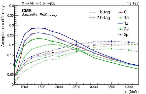
png pdf	Figure 1: Signal efficiency separated by final state and b-tagging multiplicity after the selections described in Section 5.
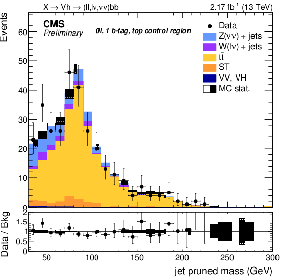
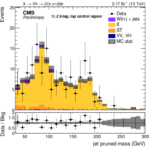
png pdf	Figure 2-a: Pruned jet mass distribution of the leading AK8 jet in the zero-lepton (a,b) and single-lepton (c,d) top quark control regions, in the 1 b-tag (a,c) and 2 b-tag (b,d) categories, after the application of the scale factors reported in Table 1 to the $ {\mathrm{ t \bar{t} } } $ and $ {\text {ST}} $ backgrounds.
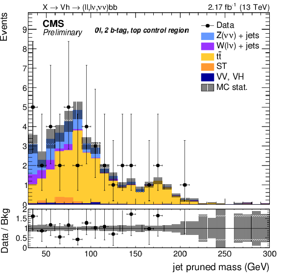
png pdf	Figure 2-b: Pruned jet mass distribution of the leading AK8 jet in the zero-lepton (a,b) and single-lepton (c,d) top quark control regions, in the 1 b-tag (a,c) and 2 b-tag (b,d) categories, after the application of the scale factors reported in Table 1 to the $ {\mathrm{ t \bar{t} } } $ and $ {\text {ST}} $ backgrounds.
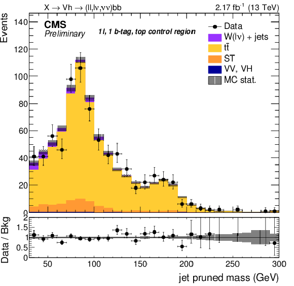
png pdf	Figure 2-c: Pruned jet mass distribution of the leading AK8 jet in the zero-lepton (a,b) and single-lepton (c,d) top quark control regions, in the 1 b-tag (a,c) and 2 b-tag (b,d) categories, after the application of the scale factors reported in Table 1 to the $ {\mathrm{ t \bar{t} } } $ and $ {\text {ST}} $ backgrounds.
png pdf	Figure 2-d: Pruned jet mass distribution of the leading AK8 jet in the zero-lepton (a,b) and single-lepton (c,d) top quark control regions, in the 1 b-tag (a,c) and 2 b-tag (b,d) categories, after the application of the scale factors reported in Table 1 to the $ {\mathrm{ t \bar{t} } } $ and $ {\text {ST}} $ backgrounds.
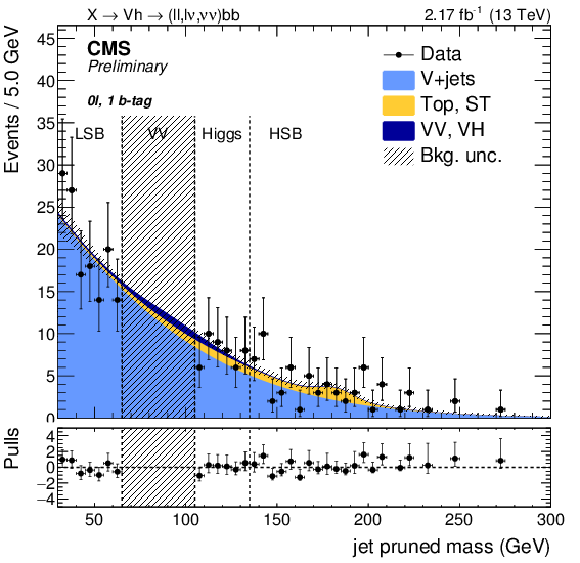
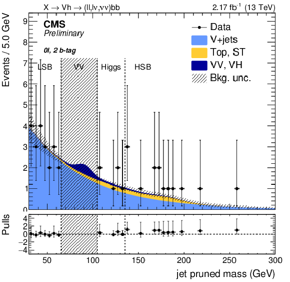
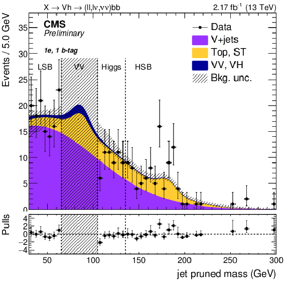
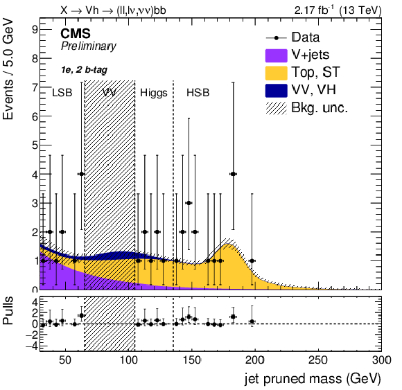
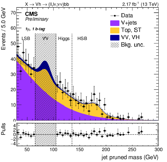
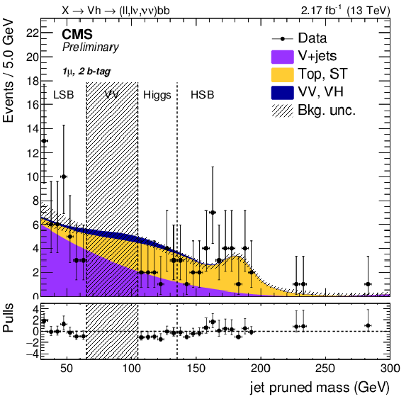
png pdf	Figure 3-a: Functional forms modeling the pruned jet mass distributions extracted from a fit to data ($ { {\mathrm {V}} \text {+jets}} $) or derived from simulation ($ {\mathrm{ t \bar{t} } } $ and $ { {\mathrm {V}} {\mathrm {V}} } $) in the zero (a,b), single electron (c,d) and single muon (e,f) lepton categories, and separately for the single (a,c,e) and double (b,d,f) b-tagging selections. The shaded area represents the $ { {\mathrm {V}} \text {+jets}} $ distribution uncertainty. In the hatched region data is omitted to avoid biasing future $ {\mathrm {X}} \to { {\mathrm {V}} {\mathrm {V}} } $ searches. The bottom panels report the pulls distribution between data and SM background expectation $(N^{data}-N^{bkg})/\sigma $, where $\sigma $ is the normalized Poisson error on the data.
png pdf	Figure 3-b: Functional forms modeling the pruned jet mass distributions extracted from a fit to data ($ { {\mathrm {V}} \text {+jets}} $) or derived from simulation ($ {\mathrm{ t \bar{t} } } $ and $ { {\mathrm {V}} {\mathrm {V}} } $) in the zero (a,b), single electron (c,d) and single muon (e,f) lepton categories, and separately for the single (a,c,e) and double (b,d,f) b-tagging selections. The shaded area represents the $ { {\mathrm {V}} \text {+jets}} $ distribution uncertainty. In the hatched region data is omitted to avoid biasing future $ {\mathrm {X}} \to { {\mathrm {V}} {\mathrm {V}} } $ searches. The bottom panels report the pulls distribution between data and SM background expectation $(N^{data}-N^{bkg})/\sigma $, where $\sigma $ is the normalized Poisson error on the data.
png pdf	Figure 3-c: Functional forms modeling the pruned jet mass distributions extracted from a fit to data ($ { {\mathrm {V}} \text {+jets}} $) or derived from simulation ($ {\mathrm{ t \bar{t} } } $ and $ { {\mathrm {V}} {\mathrm {V}} } $) in the zero (a,b), single electron (c,d) and single muon (e,f) lepton categories, and separately for the single (a,c,e) and double (b,d,f) b-tagging selections. The shaded area represents the $ { {\mathrm {V}} \text {+jets}} $ distribution uncertainty. In the hatched region data is omitted to avoid biasing future $ {\mathrm {X}} \to { {\mathrm {V}} {\mathrm {V}} } $ searches. The bottom panels report the pulls distribution between data and SM background expectation $(N^{data}-N^{bkg})/\sigma $, where $\sigma $ is the normalized Poisson error on the data.
png pdf	Figure 3-d: Functional forms modeling the pruned jet mass distributions extracted from a fit to data ($ { {\mathrm {V}} \text {+jets}} $) or derived from simulation ($ {\mathrm{ t \bar{t} } } $ and $ { {\mathrm {V}} {\mathrm {V}} } $) in the zero (a,b), single electron (c,d) and single muon (e,f) lepton categories, and separately for the single (a,c,e) and double (b,d,f) b-tagging selections. The shaded area represents the $ { {\mathrm {V}} \text {+jets}} $ distribution uncertainty. In the hatched region data is omitted to avoid biasing future $ {\mathrm {X}} \to { {\mathrm {V}} {\mathrm {V}} } $ searches. The bottom panels report the pulls distribution between data and SM background expectation $(N^{data}-N^{bkg})/\sigma $, where $\sigma $ is the normalized Poisson error on the data.
png pdf	Figure 3-e: Functional forms modeling the pruned jet mass distributions extracted from a fit to data ($ { {\mathrm {V}} \text {+jets}} $) or derived from simulation ($ {\mathrm{ t \bar{t} } } $ and $ { {\mathrm {V}} {\mathrm {V}} } $) in the zero (a,b), single electron (c,d) and single muon (e,f) lepton categories, and separately for the single (a,c,e) and double (b,d,f) b-tagging selections. The shaded area represents the $ { {\mathrm {V}} \text {+jets}} $ distribution uncertainty. In the hatched region data is omitted to avoid biasing future $ {\mathrm {X}} \to { {\mathrm {V}} {\mathrm {V}} } $ searches. The bottom panels report the pulls distribution between data and SM background expectation $(N^{data}-N^{bkg})/\sigma $, where $\sigma $ is the normalized Poisson error on the data.
png pdf	Figure 3-f: Functional forms modeling the pruned jet mass distributions extracted from a fit to data ($ { {\mathrm {V}} \text {+jets}} $) or derived from simulation ($ {\mathrm{ t \bar{t} } } $ and $ { {\mathrm {V}} {\mathrm {V}} } $) in the zero (a,b), single electron (c,d) and single muon (e,f) lepton categories, and separately for the single (a,c,e) and double (b,d,f) b-tagging selections. The shaded area represents the $ { {\mathrm {V}} \text {+jets}} $ distribution uncertainty. In the hatched region data is omitted to avoid biasing future $ {\mathrm {X}} \to { {\mathrm {V}} {\mathrm {V}} } $ searches. The bottom panels report the pulls distribution between data and SM background expectation $(N^{data}-N^{bkg})/\sigma $, where $\sigma $ is the normalized Poisson error on the data.
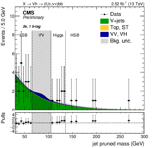
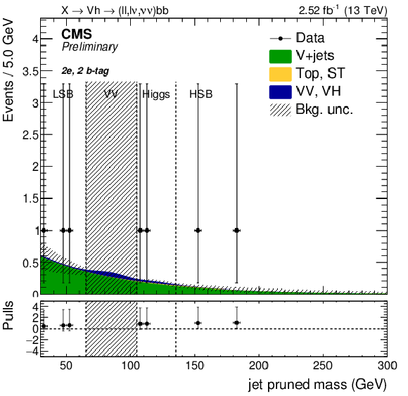
png pdf	Figure 4-a: Functional forms modeling the pruned jet mass distributions extracted from a fit to data ($ { {\mathrm {V}} \text {+jets}} $) or derived from simulation ($ {\mathrm{ t \bar{t} } } $ and $ { {\mathrm {V}} {\mathrm {V}} } $) in the double electron (a,b) and double muon (c,d) categories, and separately for the single (a,c) and double (b,d) b-tagging selections. The shaded area represents the $ { {\mathrm {V}} \text {+jets}} $ distribution uncertainty. In the hatched region data is omitted to avoid biasing future $ {\mathrm {X}} \to { {\mathrm {V}} {\mathrm {V}} } $ searches. The bottom panels report the pulls distribution between data and SM background expectation $(N^{data}-N^{bkg})/\sigma $, where $\sigma $ is the normalized Poisson error on the data.
png pdf	Figure 4-b: Functional forms modeling the pruned jet mass distributions extracted from a fit to data ($ { {\mathrm {V}} \text {+jets}} $) or derived from simulation ($ {\mathrm{ t \bar{t} } } $ and $ { {\mathrm {V}} {\mathrm {V}} } $) in the double electron (a,b) and double muon (c,d) categories, and separately for the single (a,c) and double (b,d) b-tagging selections. The shaded area represents the $ { {\mathrm {V}} \text {+jets}} $ distribution uncertainty. In the hatched region data is omitted to avoid biasing future $ {\mathrm {X}} \to { {\mathrm {V}} {\mathrm {V}} } $ searches. The bottom panels report the pulls distribution between data and SM background expectation $(N^{data}-N^{bkg})/\sigma $, where $\sigma $ is the normalized Poisson error on the data.
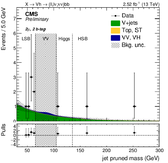
png pdf	Figure 4-c: Functional forms modeling the pruned jet mass distributions extracted from a fit to data ($ { {\mathrm {V}} \text {+jets}} $) or derived from simulation ($ {\mathrm{ t \bar{t} } } $ and $ { {\mathrm {V}} {\mathrm {V}} } $) in the double electron (a,b) and double muon (c,d) categories, and separately for the single (a,c) and double (b,d) b-tagging selections. The shaded area represents the $ { {\mathrm {V}} \text {+jets}} $ distribution uncertainty. In the hatched region data is omitted to avoid biasing future $ {\mathrm {X}} \to { {\mathrm {V}} {\mathrm {V}} } $ searches. The bottom panels report the pulls distribution between data and SM background expectation $(N^{data}-N^{bkg})/\sigma $, where $\sigma $ is the normalized Poisson error on the data.
png pdf	Figure 4-d: Functional forms modeling the pruned jet mass distributions extracted from a fit to data ($ { {\mathrm {V}} \text {+jets}} $) or derived from simulation ($ {\mathrm{ t \bar{t} } } $ and $ { {\mathrm {V}} {\mathrm {V}} } $) in the double electron (a,b) and double muon (c,d) categories, and separately for the single (a,c) and double (b,d) b-tagging selections. The shaded area represents the $ { {\mathrm {V}} \text {+jets}} $ distribution uncertainty. In the hatched region data is omitted to avoid biasing future $ {\mathrm {X}} \to { {\mathrm {V}} {\mathrm {V}} } $ searches. The bottom panels report the pulls distribution between data and SM background expectation $(N^{data}-N^{bkg})/\sigma $, where $\sigma $ is the normalized Poisson error on the data.
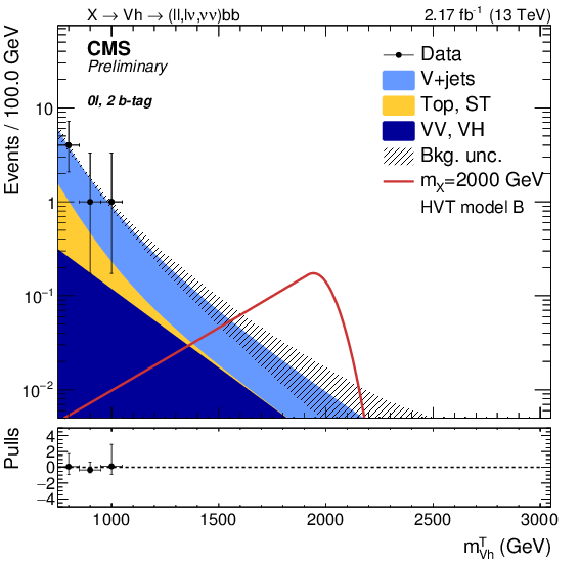
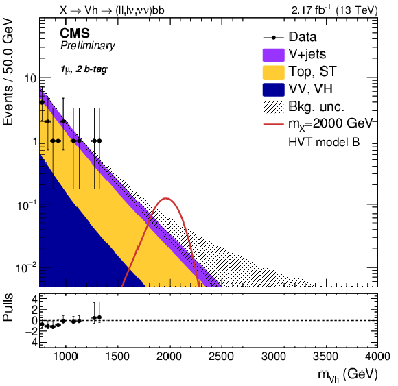
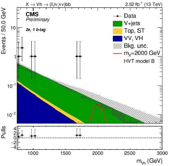
png pdf	Figure 5-a: Expected and observed events on the resonance candidate mass $ {m_{ { {\mathrm {V}} \mathrm{ h } } }} $ distributions in the zero (a,b), single electron (c,d) and single muon (e,f) categories, and separately for the single (a,c,e) and double (b,d,f) b-tagging selections. The shaded area represents the shape uncertainty on the $ { {\mathrm {V}} \text {+jets}} $ background. The pulls are reported at the bottom of each panel.
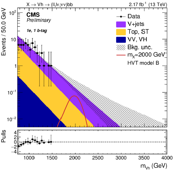
png pdf	Figure 5-b: Expected and observed events on the resonance candidate mass $ {m_{ { {\mathrm {V}} \mathrm{ h } } }} $ distributions in the zero (a,b), single electron (c,d) and single muon (e,f) categories, and separately for the single (a,c,e) and double (b,d,f) b-tagging selections. The shaded area represents the shape uncertainty on the $ { {\mathrm {V}} \text {+jets}} $ background. The pulls are reported at the bottom of each panel.
png pdf	Figure 5-c: Expected and observed events on the resonance candidate mass $ {m_{ { {\mathrm {V}} \mathrm{ h } } }} $ distributions in the zero (a,b), single electron (c,d) and single muon (e,f) categories, and separately for the single (a,c,e) and double (b,d,f) b-tagging selections. The shaded area represents the shape uncertainty on the $ { {\mathrm {V}} \text {+jets}} $ background. The pulls are reported at the bottom of each panel.
png pdf	Figure 5-d: Expected and observed events on the resonance candidate mass $ {m_{ { {\mathrm {V}} \mathrm{ h } } }} $ distributions in the zero (a,b), single electron (c,d) and single muon (e,f) categories, and separately for the single (a,c,e) and double (b,d,f) b-tagging selections. The shaded area represents the shape uncertainty on the $ { {\mathrm {V}} \text {+jets}} $ background. The pulls are reported at the bottom of each panel.
png pdf	Figure 5-e: Expected and observed events on the resonance candidate mass $ {m_{ { {\mathrm {V}} \mathrm{ h } } }} $ distributions in the zero (a,b), single electron (c,d) and single muon (e,f) categories, and separately for the single (a,c,e) and double (b,d,f) b-tagging selections. The shaded area represents the shape uncertainty on the $ { {\mathrm {V}} \text {+jets}} $ background. The pulls are reported at the bottom of each panel.
png pdf	Figure 5-f: Expected and observed events on the resonance candidate mass $ {m_{ { {\mathrm {V}} \mathrm{ h } } }} $ distributions in the zero (a,b), single electron (c,d) and single muon (e,f) categories, and separately for the single (a,c,e) and double (b,d,f) b-tagging selections. The shaded area represents the shape uncertainty on the $ { {\mathrm {V}} \text {+jets}} $ background. The pulls are reported at the bottom of each panel.
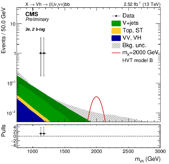
png pdf	Figure 6-a: Expected and observed events on the resonance candidate mass $ {m_{ { {\mathrm {V}} \mathrm{ h } } }} $ distributions in the double electron (a,b) and double muon (c,d) categories, and separately for the single (a,c) and double (b,d) b-tagging selections. The shaded area represents the shape uncertainty on the $ { {\mathrm {V}} \text {+jets}} $ background. The pulls are reported at the bottom of each panel.
png pdf	Figure 6-b: Expected and observed events on the resonance candidate mass $ {m_{ { {\mathrm {V}} \mathrm{ h } } }} $ distributions in the double electron (a,b) and double muon (c,d) categories, and separately for the single (a,c) and double (b,d) b-tagging selections. The shaded area represents the shape uncertainty on the $ { {\mathrm {V}} \text {+jets}} $ background. The pulls are reported at the bottom of each panel.
png pdf	Figure 6-c: Expected and observed events on the resonance candidate mass $ {m_{ { {\mathrm {V}} \mathrm{ h } } }} $ distributions in the double electron (a,b) and double muon (c,d) categories, and separately for the single (a,c) and double (b,d) b-tagging selections. The shaded area represents the shape uncertainty on the $ { {\mathrm {V}} \text {+jets}} $ background. The pulls are reported at the bottom of each panel.
png pdf	Figure 6-d: Expected and observed events on the resonance candidate mass $ {m_{ { {\mathrm {V}} \mathrm{ h } } }} $ distributions in the double electron (a,b) and double muon (c,d) categories, and separately for the single (a,c) and double (b,d) b-tagging selections. The shaded area represents the shape uncertainty on the $ { {\mathrm {V}} \text {+jets}} $ background. The pulls are reported at the bottom of each panel.
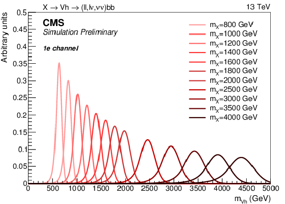
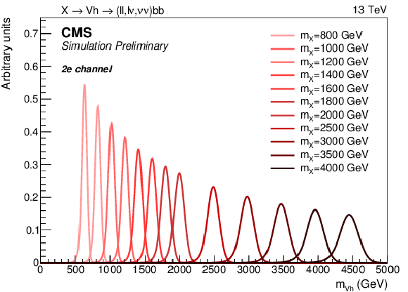
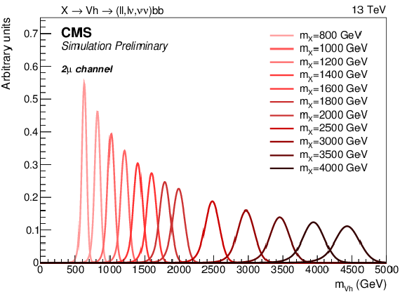
png pdf	Figure 7-a: Reconstructed signal mass $ {m_{ { {\mathrm {V}} \mathrm{ h } } }} $ for different generated mass $ {m_{ {\mathrm {X}} }} $ hypotheses, modeled with a Crystal Ball function, and separately by final state: zero leptons (a), single electron (b), single muon (c), double electron (d ), and double muon (e) categories. The single and double b-tag categories are merged together. The distributions are normalized to the unit area.
png pdf	Figure 7-b: Reconstructed signal mass $ {m_{ { {\mathrm {V}} \mathrm{ h } } }} $ for different generated mass $ {m_{ {\mathrm {X}} }} $ hypotheses, modeled with a Crystal Ball function, and separately by final state: zero leptons (a), single electron (b), single muon (c), double electron (d ), and double muon (e) categories. The single and double b-tag categories are merged together. The distributions are normalized to the unit area.
png pdf	Figure 7-c: Reconstructed signal mass $ {m_{ { {\mathrm {V}} \mathrm{ h } } }} $ for different generated mass $ {m_{ {\mathrm {X}} }} $ hypotheses, modeled with a Crystal Ball function, and separately by final state: zero leptons (a), single electron (b), single muon (c), double electron (d ), and double muon (e) categories. The single and double b-tag categories are merged together. The distributions are normalized to the unit area.
png pdf	Figure 7-d: Reconstructed signal mass $ {m_{ { {\mathrm {V}} \mathrm{ h } } }} $ for different generated mass $ {m_{ {\mathrm {X}} }} $ hypotheses, modeled with a Crystal Ball function, and separately by final state: zero leptons (a), single electron (b), single muon (c), double electron (d ), and double muon (e) categories. The single and double b-tag categories are merged together. The distributions are normalized to the unit area.
png pdf	Figure 7-e: Reconstructed signal mass $ {m_{ { {\mathrm {V}} \mathrm{ h } } }} $ for different generated mass $ {m_{ {\mathrm {X}} }} $ hypotheses, modeled with a Crystal Ball function, and separately by final state: zero leptons (a), single electron (b), single muon (c), double electron (d ), and double muon (e) categories. The single and double b-tag categories are merged together. The distributions are normalized to the unit area.
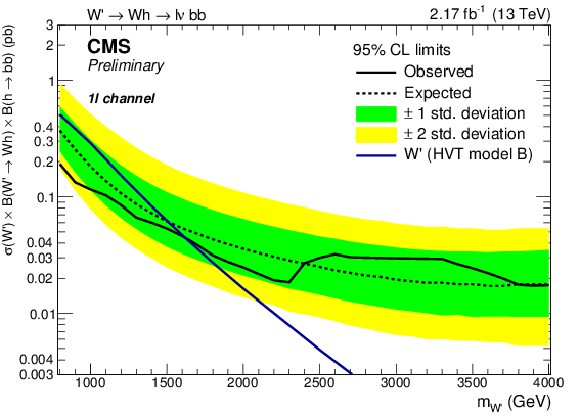
png pdf	Figure 8-a: Observed and expected 95% CL upper limit on $\sigma _ {\mathrm {X}} \times {\mathcal {B}}( {\mathrm {X}} \to { {\mathrm {V}} \mathrm{ h } } ) \times {\mathcal {B}}( {\mathrm{ h } \to \mathrm{ b \bar{b} } } )$ as a function of the resonance mass for a narrow spin-1 resonance, including all statistical and systematic uncertainties, for the $ {\mathrm {X}} \to {\mathrm{ Z } } {\mathrm {h}} $ (a) and $ {\mathrm {X}} \to {\mathrm {W}} {\mathrm {h}} $ (b) decay channels. The green and yellow bands are the ${\pm }$1 and ${\pm }$2 standard deviation uncertainty bands on the expected limit.
png pdf	Figure 8-b: Observed and expected 95% CL upper limit on $\sigma _ {\mathrm {X}} \times {\mathcal {B}}( {\mathrm {X}} \to { {\mathrm {V}} \mathrm{ h } } ) \times {\mathcal {B}}( {\mathrm{ h } \to \mathrm{ b \bar{b} } } )$ as a function of the resonance mass for a narrow spin-1 resonance, including all statistical and systematic uncertainties, for the $ {\mathrm {X}} \to {\mathrm{ Z } } {\mathrm {h}} $ (a) and $ {\mathrm {X}} \to {\mathrm {W}} {\mathrm {h}} $ (b) decay channels. The green and yellow bands are the ${\pm }$1 and ${\pm }$2 standard deviation uncertainty bands on the expected limit.

Tables
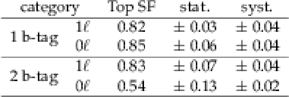
png pdf	Table 1: Top normalization scale factors, reported independently for each channel. Electron and muon categories are merged. Uncertainties are both due to the limited statistics in data (stat.) and the systematic uncertainty on the b-tagging efficiency (syst.).
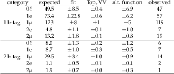
png pdf	Table 2: Expected and observed number of events in the SR (105 $< m_j <$ 135 GeV). The uncertainties originating from the fit and the top and diboson $ {m_{\mathrm{j}}} $ distributions are reported separately, as well as the difference in normalization between the nominal and the alternative function choice.
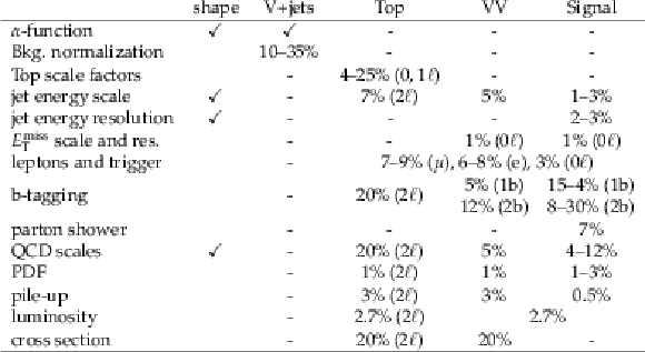
png pdf	Table 3: Summary of systematic uncertainties for backgrounds and signal samples. The top quark background normalization uncertainties are divided depending on the final state. The uncertainty sources propagated to the $ {m_{ { {\mathrm {V h } } } }} $ shape are marked with a tick.

Summary

This note described a search for a heavy resonance with mass between 800 GeV and 4 TeV, decaying into a vector boson and a Higgs boson. The data collected at $\sqrt{s}=$ 13 TeV during the 2015 operations by the CMS experiment at LHC Run-2 are analyzed. The data set size corresponds to an integrated luminosity of 2.17-2.52 fb$^{-1}$, depending on the channel. The final states explored include all the leptonic decay modes of the vector boson, in events with zero ($\mathrm{Z} \to \nu\nu$), exactly one ($\mathrm{W} \to \ell\nu$) and two ($\mathrm{Z} \to \ell\ell$) leptons. Higgs bosons are reconstructed from their decays to $\mathrm{ b \bar{b} }$ pairs. Depending on the resonance mass, an upper limit of 10-200 fb is set on the cross section of a spin-1 narrow resonance multiplied by the branching ratio of the resonance in a Higgs boson and a vector boson, and the branching ratio of the Higgs boson to b quarks.

Additional Figures
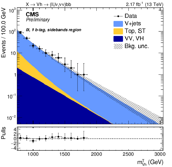
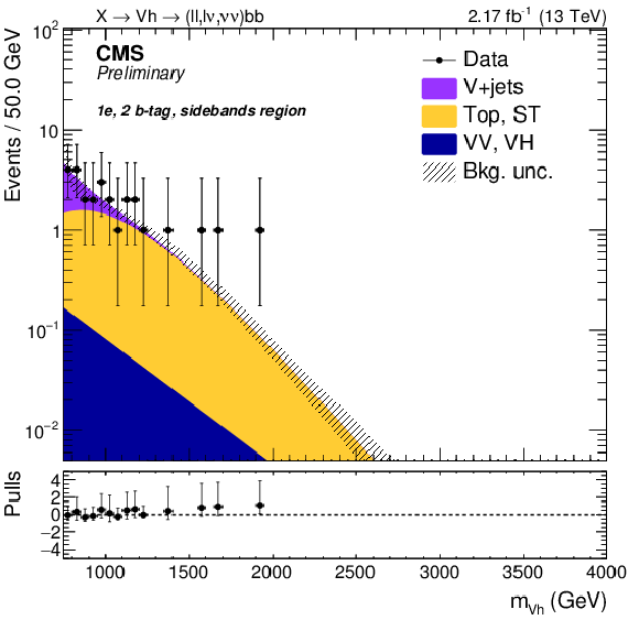
png pdf	Additional Figure 1-a: Expected and observed events in the $m_j$ sidebands on the resonance candidate mass $m_{\mathrm{Vh}}$ distributions in the zero (a,b), single electron (c,d) and single muon (e,f) categories, and separately for the single (a,c,e) and double (b,d,f) b-tagging selections. The shaded area represents the shape uncertainty on the V+jets background. The pulls are reported at the bottom of each panel.
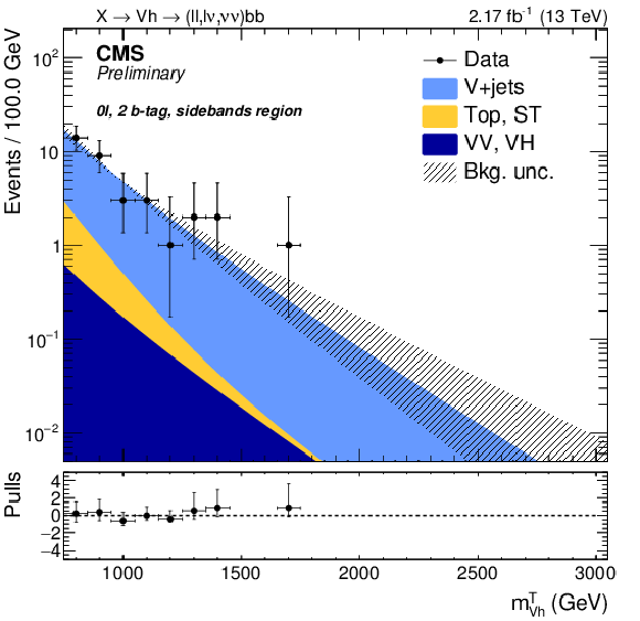
png pdf	Additional Figure 1-b: Expected and observed events in the $m_j$ sidebands on the resonance candidate mass $m_{\mathrm{Vh}}$ distributions in the zero (a,b), single electron (c,d) and single muon (e,f) categories, and separately for the single (a,c,e) and double (b,d,f) b-tagging selections. The shaded area represents the shape uncertainty on the V+jets background. The pulls are reported at the bottom of each panel.
png pdf	Additional Figure 1-c: Expected and observed events in the $m_j$ sidebands on the resonance candidate mass $m_{\mathrm{Vh}}$ distributions in the zero (a,b), single electron (c,d) and single muon (e,f) categories, and separately for the single (a,c,e) and double (b,d,f) b-tagging selections. The shaded area represents the shape uncertainty on the V+jets background. The pulls are reported at the bottom of each panel.
png pdf	Additional Figure 1-d: Expected and observed events in the $m_j$ sidebands on the resonance candidate mass $m_{\mathrm{Vh}}$ distributions in the zero (a,b), single electron (c,d) and single muon (e,f) categories, and separately for the single (a,c,e) and double (b,d,f) b-tagging selections. The shaded area represents the shape uncertainty on the V+jets background. The pulls are reported at the bottom of each panel.
png pdf	Additional Figure 1-e: Expected and observed events in the $m_j$ sidebands on the resonance candidate mass $m_{\mathrm{Vh}}$ distributions in the zero (a,b), single electron (c,d) and single muon (e,f) categories, and separately for the single (a,c,e) and double (b,d,f) b-tagging selections. The shaded area represents the shape uncertainty on the V+jets background. The pulls are reported at the bottom of each panel.
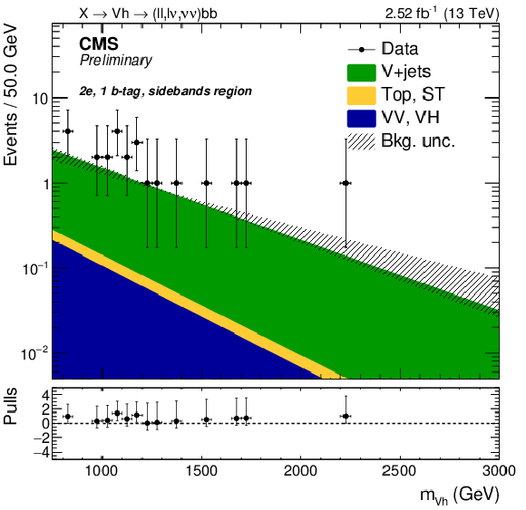
png pdf	Additional Figure 1-f: Expected and observed events in the $m_j$ sidebands on the resonance candidate mass $m_{\mathrm{Vh}}$ distributions in the zero (a,b), single electron (c,d) and single muon (e,f) categories, and separately for the single (a,c,e) and double (b,d,f) b-tagging selections. The shaded area represents the shape uncertainty on the V+jets background. The pulls are reported at the bottom of each panel.
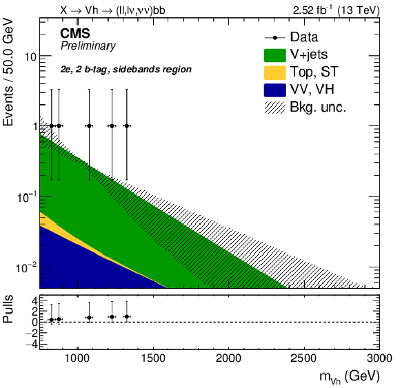
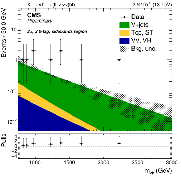
png pdf	Additional Figure 2-a: Expected and observed events in the $m_j$ sidebands on the resonance candidate mass $m_{\mathrm{Vh}}$ distributions in the double electron (a,b) and double muon (c,d) categories, and separately for the single (a,c) and double (b,d) b-tagging selections. The shaded area represents the shape uncertainty on the V+jets background. The pulls are reported at the bottom of each panel.
png pdf	Additional Figure 2-b: Expected and observed events in the $m_j$ sidebands on the resonance candidate mass $m_{\mathrm{Vh}}$ distributions in the double electron (a,b) and double muon (c,d) categories, and separately for the single (a,c) and double (b,d) b-tagging selections. The shaded area represents the shape uncertainty on the V+jets background. The pulls are reported at the bottom of each panel.
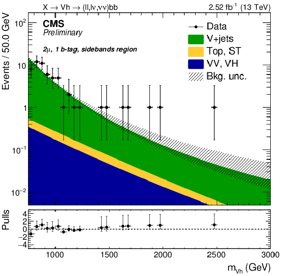
png pdf	Additional Figure 2-c: Expected and observed events in the $m_j$ sidebands on the resonance candidate mass $m_{\mathrm{Vh}}$ distributions in the double electron (a,b) and double muon (c,d) categories, and separately for the single (a,c) and double (b,d) b-tagging selections. The shaded area represents the shape uncertainty on the V+jets background. The pulls are reported at the bottom of each panel.
png pdf	Additional Figure 2-d: Expected and observed events in the $m_j$ sidebands on the resonance candidate mass $m_{\mathrm{Vh}}$ distributions in the double electron (a,b) and double muon (c,d) categories, and separately for the single (a,c) and double (b,d) b-tagging selections. The shaded area represents the shape uncertainty on the V+jets background. The pulls are reported at the bottom of each panel.
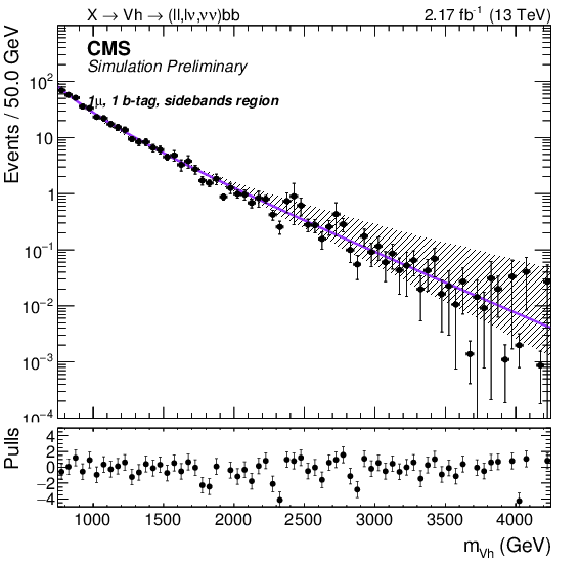
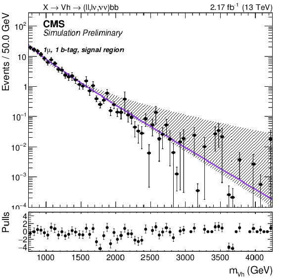
png pdf	Additional Figure 3-a: Fits to the $m_{\mathrm{Vh}}$ distribution of V+jets simulated samples with a two-parameter function in the jet mass sidebands (a) and signal region (b) for events passing the single muon, single b-tag category selections. The shaded area corresponds to the fit uncertainty.
png pdf	Additional Figure 3-b: Fits to the $m_{\mathrm{Vh}}$ distribution of V+jets simulated samples with a two-parameter function in the jet mass sidebands (a) and signal region (b) for events passing the single muon, single b-tag category selections. The shaded area corresponds to the fit uncertainty.
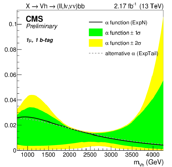
png pdf	Additional Figure 4: $\alpha (m_{\mathrm{Vh}})$ function, defined as the ratio of the $m_{\mathrm{Vh}}$ distributions in the signal region and the sidebands, extracted from V+jets simulated events. The function is referred to the single muon, single b-tag category. The green and yellow uncertainty bands are derived by propagating the corresponding uncertainties from the fits to the signal and sideband regions. The dotted line represents the $\alpha $ function obtained with an alternative function choice.
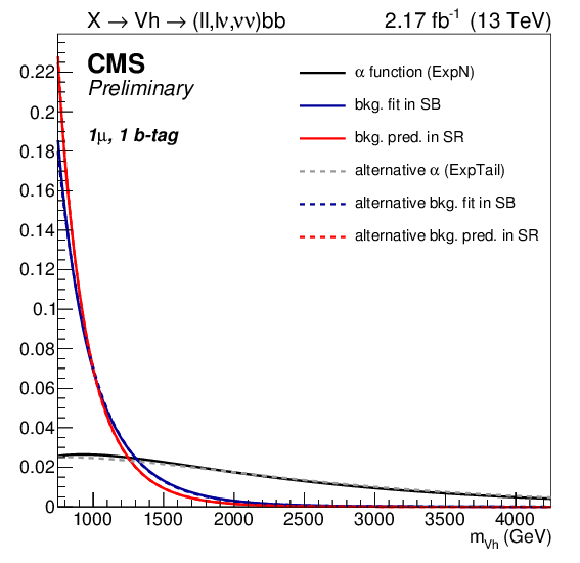
png pdf	Additional Figure 5-a: Visualization of the $\alpha $ ratio method in the linear (a) and logarithmic scale (b). The blue line represents the V+jets component from the fit to data in the sidebands regions. The black line is the $\alpha $ function, defined as the ratio of the $m_{\mathrm{Vh}}$ distributions in the signal region and the sidebands, extracted from V+jets simulated events. The red line is the V+jets background prediction in the signal region, obtained by multiplying the shape in the sidebands (blue line) with the $\alpha $ ratio (black line). The dotted lines represent the same quantities but extracted with the alternative function choice.
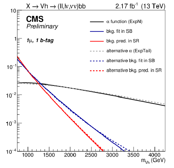
png pdf	Additional Figure 5-b: Visualization of the $\alpha $ ratio method in the linear (a) and logarithmic scale (b). The blue line represents the V+jets component from the fit to data in the sidebands regions. The black line is the $\alpha $ function, defined as the ratio of the $m_{\mathrm{Vh}}$ distributions in the signal region and the sidebands, extracted from V+jets simulated events. The red line is the V+jets background prediction in the signal region, obtained by multiplying the shape in the sidebands (blue line) with the $\alpha $ ratio (black line). The dotted lines represent the same quantities but extracted with the alternative function choice.
png pdf	Additional Figure 6: Observed and expected 95% CL upper limit on $\sigma _{\mathrm{X}} \times \mathcal {B}(\mathrm{ X \to Zh }) \times \mathcal {B}(\mathrm{ h } \to \mathrm{ b \bar{b} })$ as a function of $m_{\mathrm{Vh}}$ for a narrow spin-1 resonance for the $\mathrm{ X \to Zh }$, ${\mathrm{ Z } } \to \nu \nu $ decay channel. The single and double b-tag categories are combined together. The green and yellow bands are the ${\pm }1$ and ${\pm }2$ standard deviation uncertainty bands on the expected limit.
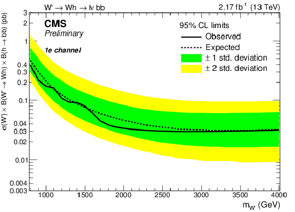
png pdf	Additional Figure 7: Observed and expected 95% CL upper limit on $\sigma _{\mathrm{X}} \times \mathcal {B}(\mathrm{ X\to Wh }) \times \mathcal {B}(\mathrm{ h } \to \mathrm{ b \bar{b} })$ as a function of $m_{\mathrm{Vh}}$ for a narrow spin-1 resonance for the $\mathrm{ X\to Wh }$, $ {\mathrm {W}} \to \mathrm{ e } \nu $ decay channel. The single and double b-tag categories are combined together. The green and yellow bands are the ${\pm }1$ and ${\pm }2$ standard deviation uncertainty bands on the expected limit.
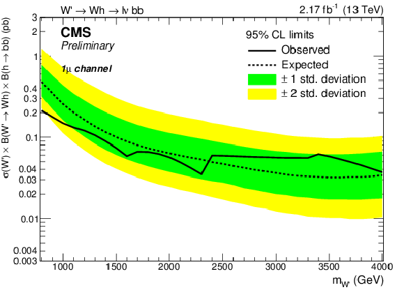
png pdf	Additional Figure 8: Observed and expected 95% CL upper limit on $\sigma _{\mathrm{X}} \times \mathcal {B}(\mathrm{ X\to Wh }) \times \mathcal {B}(\mathrm{ h } \to \mathrm{ b \bar{b} })$ as a function of $m_{\mathrm{Vh}}$ for a narrow spin-1 resonance for the $\mathrm{ X\to Wh }$, $ {\mathrm {W}} \to \mu \nu $ decay channel. The single and double b-tag categories are combined together. The green and yellow bands are the ${\pm }1$ and ${\pm }2$ standard deviation uncertainty bands on the expected limit.
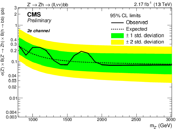
png pdf	Additional Figure 9: Observed and expected 95% CL upper limit on $\sigma _{\mathrm{X}} \times \mathcal {B}(\mathrm{ X \to Zh }) \times \mathcal {B}(\mathrm{ h } \to \mathrm{ b \bar{b} })$ as a function of $m_{\mathrm{Vh}}$ for a narrow spin-1 resonance for the $\mathrm{ X \to Zh }$, ${\mathrm{ Z } } \to \mathrm{ e } \mathrm{ e } $ decay channel. The single and double b-tag categories are combined together. The green and yellow bands are the ${\pm }1$ and ${\pm }2$ standard deviation uncertainty bands on the expected limit.
png pdf	Additional Figure 10: Observed and expected 95% CL upper limit on $\sigma _{\mathrm{X}} \times \mathcal {B}(\mathrm{ X \to Zh }) \times \mathcal {B}(\mathrm{ h } \to \mathrm{ b \bar{b} })$ as a function of $m_{\mathrm{Vh}}$ for a narrow spin-1 resonance for the $\mathrm{ X \to Zh }$, ${\mathrm{ Z } } \to \mu \mu $ decay channel. The single and double b-tag categories are combined together. The green and yellow bands are the ${\pm }1$ and ${\pm }2$ standard deviation uncertainty bands on the expected limit.