

Compact Muon Solenoid
LHC, CERN
| CMS-PAS-TOP-15-001 | ||
| Measurement of the top quark mass from single-top production events | ||
| CMS Collaboration | ||
| March 2016 | ||
| Abstract: We measure the mass of the top quark from events where a single top quark is produced. The analysis is performed on data from pp collisions collected by the CMS detector at a center of mass energy of 8 TeV. The top quark is reconstructed from its decay $\mathrm{t} \rightarrow \mathrm{W}^+ \mathrm{b}$, with the $\mathrm{W}$ boson decaying leptonically in the muon channel. Specific event topology and kinematic properties are used in order to enrich the sample in single-top-quark events in the $t$-channel, at the expense of top-quark pair production events. For the single-top quark component, a fit to the reconstructed top invariant mass distribution yields $m_{\mathrm{t}} =$ 172.60 $\pm$ 0.77 (stat) $^{+0.97}_{-0.93}$ (syst) GeV. | ||
|
Links:
CDS record (PDF) ;
CADI line (restricted) ;
These preliminary results are superseded in this paper, EPJC 77 (2017) 354. The superseded preliminary plots can be found here. |
||
| Figures | |
png pdf |
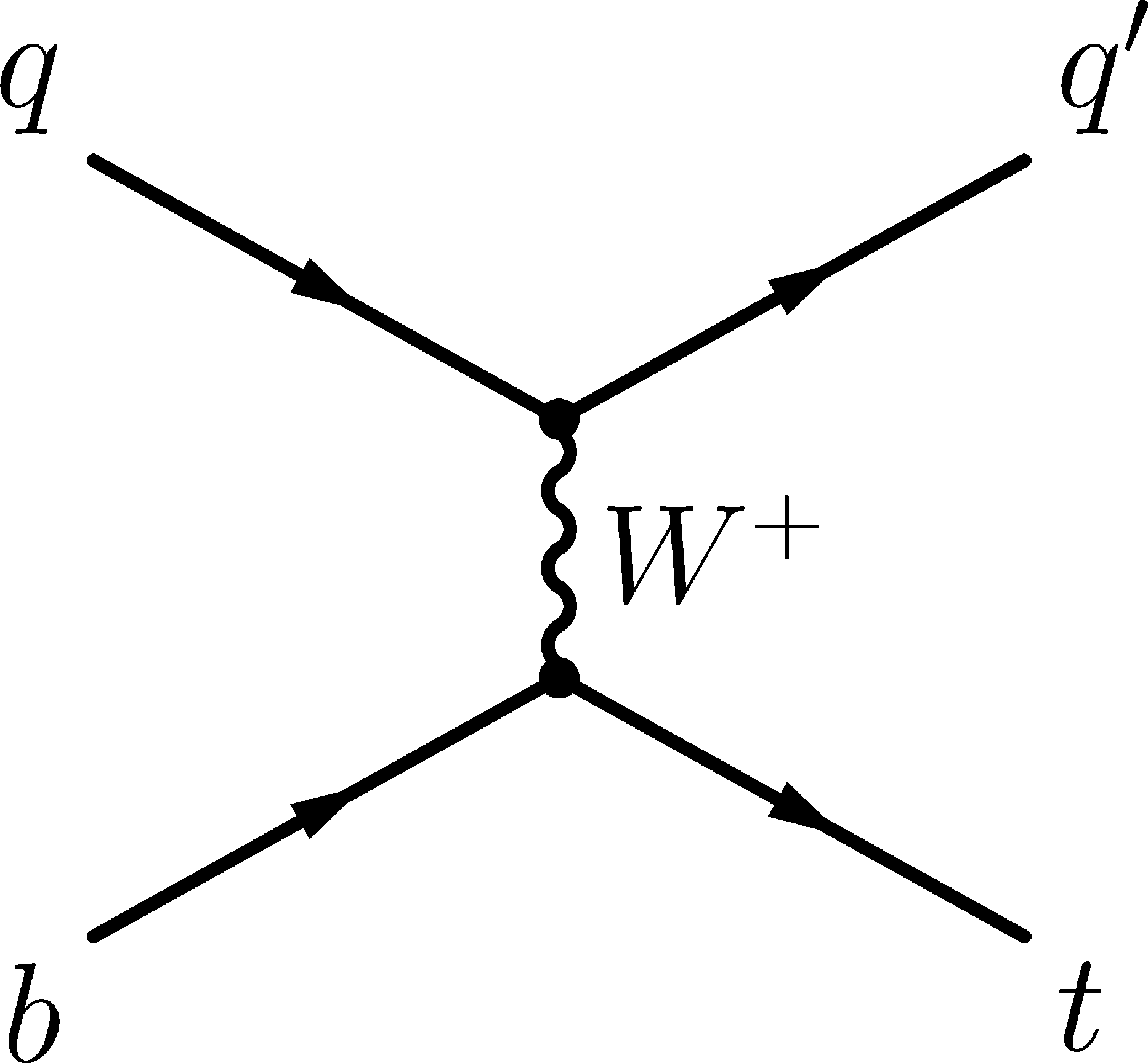
Figure 1-a:
Dominant Feynman diagrams for single top quark production in the $t$-channel in leading order five-flavour scheme 2$\rightarrow $2 (a) and next-to-leading order four-flavour scheme 2$\rightarrow $3 (b) processes. |
png pdf |
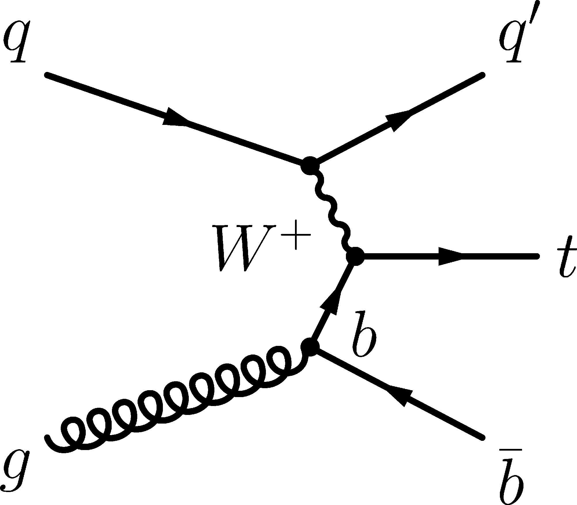
Figure 1-b:
Dominant Feynman diagrams for single top quark production in the $t$-channel in leading order five-flavour scheme 2$\rightarrow $2 (a) and next-to-leading order four-flavour scheme 2$\rightarrow $3 (b) processes. |
png |
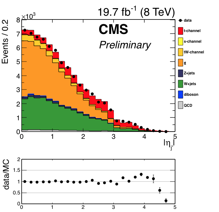
Figure 2-a:
Distribution of the light jet pseudorapidity (a) and of the reconstructed top quark charge (b). Points represent real data, stacked histograms show expected contributions from different event classes in simulated data. Bottom plots show the ratio of the observed number of events in real data to the number predicted by simulation. |
png |
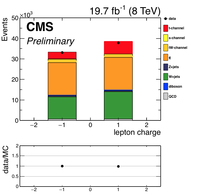
Figure 2-b:
Distribution of the light jet pseudorapidity (a) and of the reconstructed top quark charge (b). Points represent real data, stacked histograms show expected contributions from different event classes in simulated data. Bottom plots show the ratio of the observed number of events in real data to the number predicted by simulation. |
png |
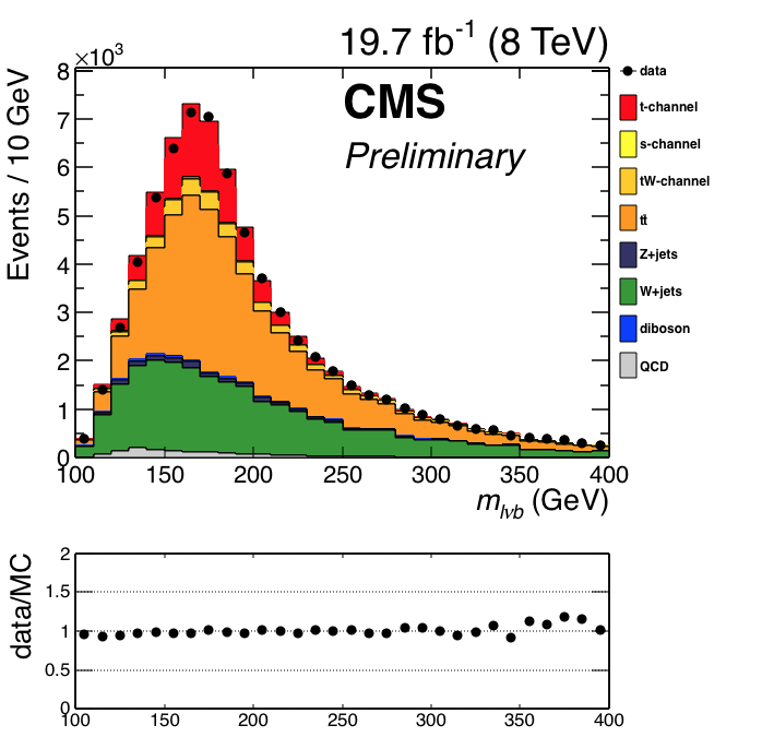
Figure 3-a:
Reconstructed top quark mass distribution for data (points) and Monte Carlo events (stacked histograms). a: initial selection; b: final selection after charge and light jet pseudorapidity cuts. Bottom plots show the ratio of the observed number of events in real data to the number predicted by simulation. |
png |
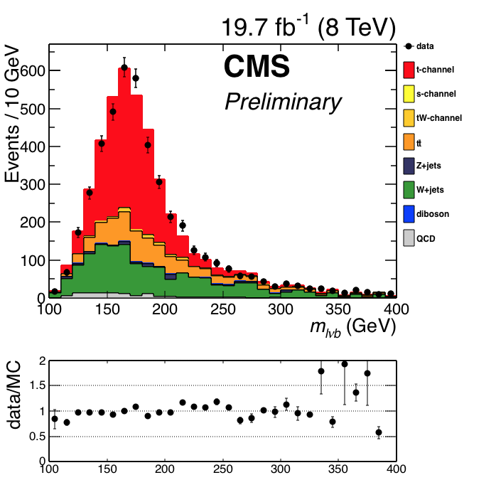
Figure 3-b:
Reconstructed top quark mass distribution for data (points) and Monte Carlo events (stacked histograms). a: initial selection; b: final selection after charge and light jet pseudorapidity cuts. Bottom plots show the ratio of the observed number of events in real data to the number predicted by simulation. |
png |
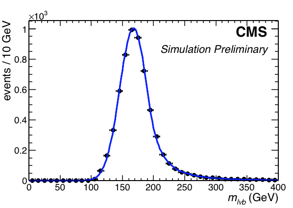
Figure 4-a:
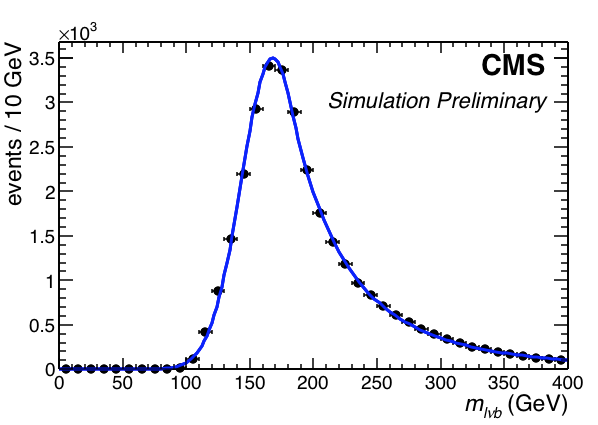
Signal shape from Monte Carlo simulation. a: single top $t$-channel events; b: $ {\mathrm{ t \bar{t} } } $ events. The continuous blue lines show the results of fits to Crystal Ball shapes. |
png |
Figure 4-b:
Signal shape from Monte Carlo simulation. a: single top $t$-channel events; b: $ {\mathrm{ t \bar{t} } } $ events. The continuous blue lines show the results of fits to Crystal Ball shapes. |
png |
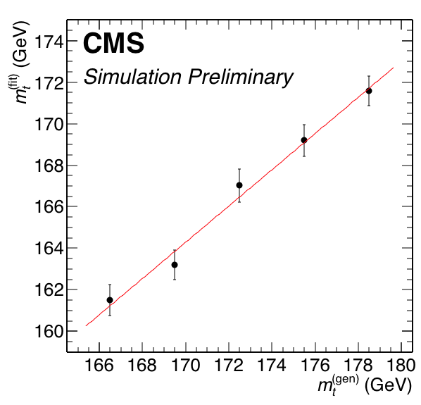
Figure 5-a:
Mass calibration from fits to samples with different generated top mass. a: fit results as a function of the generated top mass. The red line shows the result of a linear fit to the points. b: mass correction, as a function of the fitted top mass (red line). The shaded grey area represents the associated systematic uncertainty. |
png |
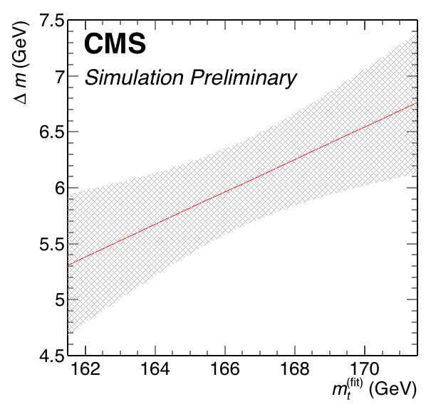
Figure 5-b:
Mass calibration from fits to samples with different generated top mass. a: fit results as a function of the generated top mass. The red line shows the result of a linear fit to the points. b: mass correction, as a function of the fitted top mass (red line). The shaded grey area represents the associated systematic uncertainty. |
png |
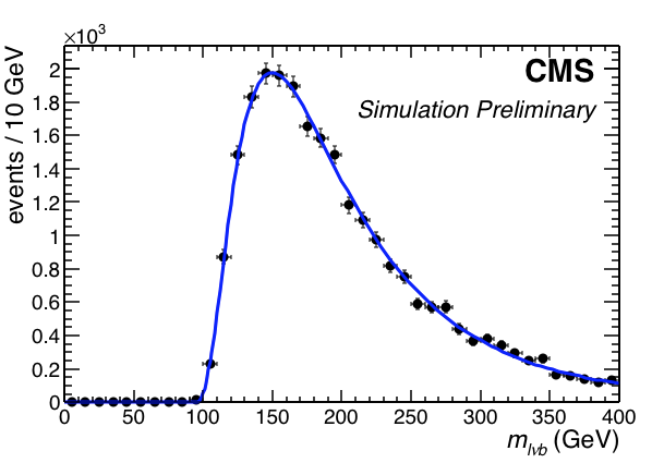
Figure 6-a:
Background shape from Monte Carlo simulation. a: before final selection; b: after final selection. The continuous blue lines show the results of fits to Novosibirsk functions. |
png |
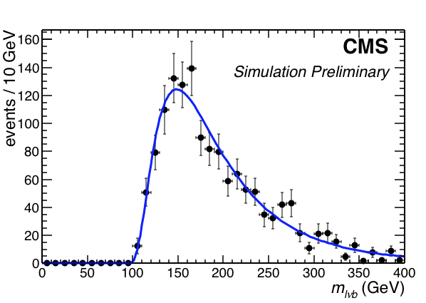
Figure 6-b:
Background shape from Monte Carlo simulation. a: before final selection; b: after final selection. The continuous blue lines show the results of fits to Novosibirsk functions. |
png |
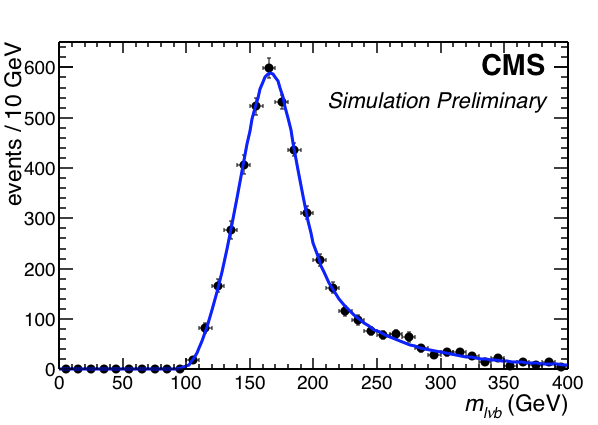
Figure 7-a:
Result of the fit to the top invariant mass shape. a: Monte Carlo; b: real data. The solid blue line represents the fitted PDF. |
png |
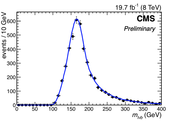
Figure 7-b:
Result of the fit to the top invariant mass shape. a: Monte Carlo; b: real data. The solid blue line represents the fitted PDF. |
| Tables | |
png pdf |
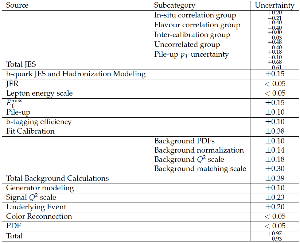
Table 1:
Systematic uncertainties on the top-quark mass, in GeV. |
|
|
Compact Muon Solenoid LHC, CERN |
|

|

|

|

|

|