

Compact Muon Solenoid
LHC, CERN
| CMS-PAS-TOP-14-023 | ||
| Measurements of $ \mathrm{ t \bar{t} } $ spin correlations and top-quark polarization using dilepton final states in pp collisions at $ \sqrt{s} = $ 8 TeV | ||
| CMS Collaboration | ||
| September 2015 | ||
| Abstract: Spin correlations and polarization are measured in top quark-antiquark pairs produced in pp collisions at the LHC at $ \sqrt{s} =$ 8 TeV. The data correspond to an integrated luminosity of 19.5 fb$^{-1}$ collected with the CMS detector. The measurements are performed using events with two oppositely charged leptons (electrons or muons) and two or more jets, where at least one of the jets is identified as originating from a b quark. The spin correlations and polarization are measured from the angular distributions of the two selected leptons, unfolded to the parton level, both inclusively and differentially with respect to the invariant mass, rapidity, and transverse momentum of the $ \mathrm{ t \bar{t} } $ system. All measurements are found to be in agreement with predictions of the standard model of particle physics. A search for new physics in the form of a top quark chromo-magnetic anomalous coupling is performed, and the measured value of the real part of the chomo-magnetic coupling $\mathrm{Re}(\hat{\mu}_t)$ is found to be $-0.013 \pm 0.032$ with a corresponding 95% confidence interval of $-0.050< \mathrm{Re}(\hat{\mu}_t) < 0.076$. | ||
|
Links:
CDS record (PDF) ;
Public twiki page ;
CADI line (restricted) ; Figures are also available from the CDS record. These preliminary results are superseded in this paper, PRD 93 (2016) 052007. |
||
| Figures | |

png ; pdf |
Figure 1-a:
The reconstructed $M_{ {\mathrm {t}\overline {\mathrm {t}}} }$ (a), $ {p_{\mathrm {T}}}^{ {\mathrm {t}\overline {\mathrm {t}}} }$ (b), and $y_{ {\mathrm {t}\overline {\mathrm {t}}} }$ (c) distributions from data (points) and simulation (histogram). All the dilepton flavour combinations are included. The simulated signal yield is normalized to that of the background-subtracted data. The first and last bins include underflow and overflow events, respectively. The error bars on the data points represent the statistical uncertainties. |
png ; pdf |
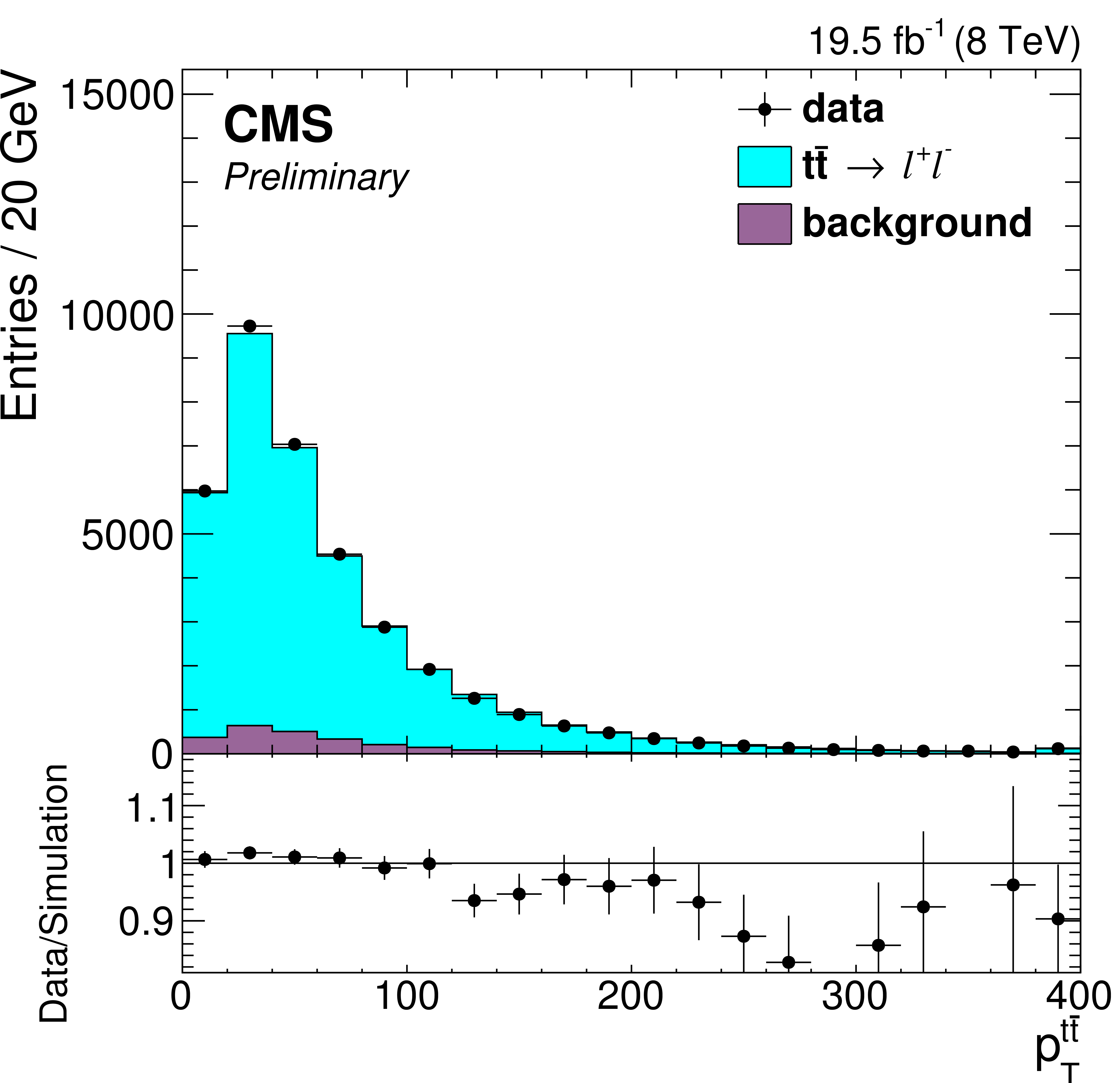
Figure 1-b:
The reconstructed $M_{ {\mathrm {t}\overline {\mathrm {t}}} }$ (a), $ {p_{\mathrm {T}}}^{ {\mathrm {t}\overline {\mathrm {t}}} }$ (b), and $y_{ {\mathrm {t}\overline {\mathrm {t}}} }$ (c) distributions from data (points) and simulation (histogram). All the dilepton flavour combinations are included. The simulated signal yield is normalized to that of the background-subtracted data. The first and last bins include underflow and overflow events, respectively. The error bars on the data points represent the statistical uncertainties. |

png ; pdf |
Figure 1-c:
The reconstructed $M_{ {\mathrm {t}\overline {\mathrm {t}}} }$ (a), $ {p_{\mathrm {T}}}^{ {\mathrm {t}\overline {\mathrm {t}}} }$ (b), and $y_{ {\mathrm {t}\overline {\mathrm {t}}} }$ (c) distributions from data (points) and simulation (histogram). All the dilepton flavour combinations are included. The simulated signal yield is normalized to that of the background-subtracted data. The first and last bins include underflow and overflow events, respectively. The error bars on the data points represent the statistical uncertainties. |

png ; pdf |
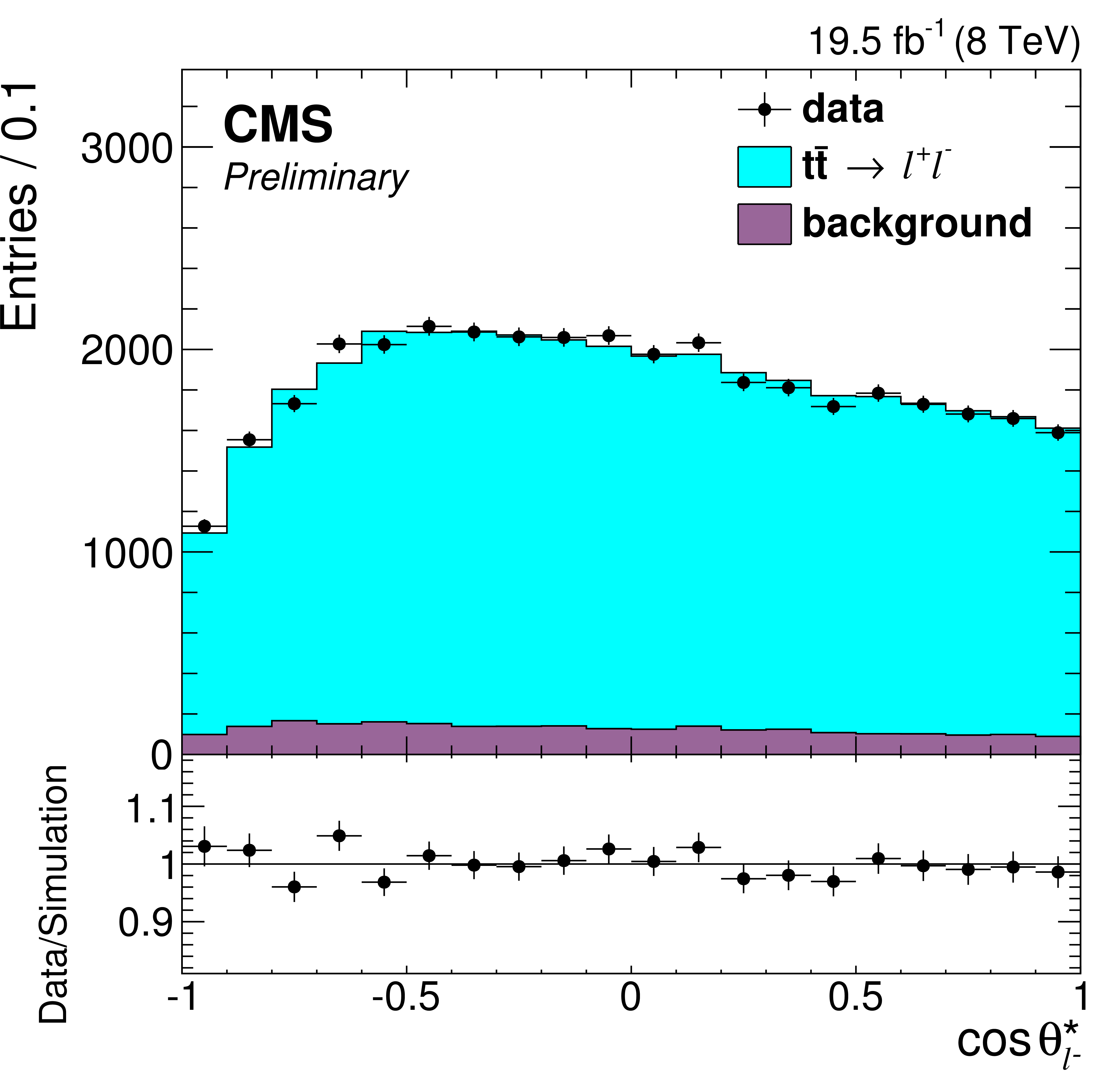
Figure 2-a:
The reconstructed angular distributions from data (points) and simulation (histogram). All the dilepton flavour combinations are included. The signal yield is normalized to the background-subtracted data. The error bars on the data points represent the statistical uncertainties. |

png ; pdf |
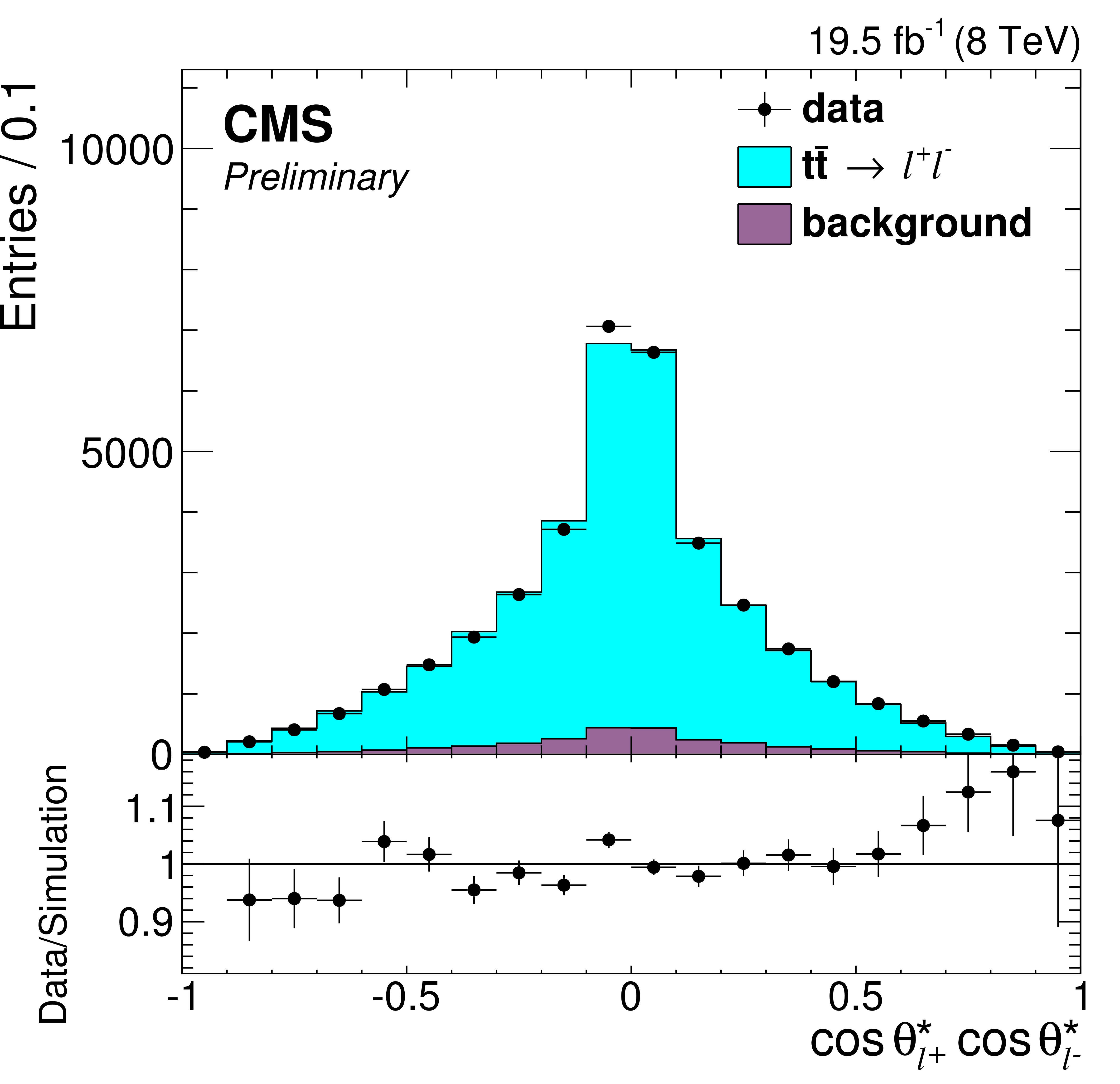
Figure 2-b:
The reconstructed angular distributions from data (points) and simulation (histogram). All the dilepton flavour combinations are included. The signal yield is normalized to the background-subtracted data. The error bars on the data points represent the statistical uncertainties. |
png ; pdf |
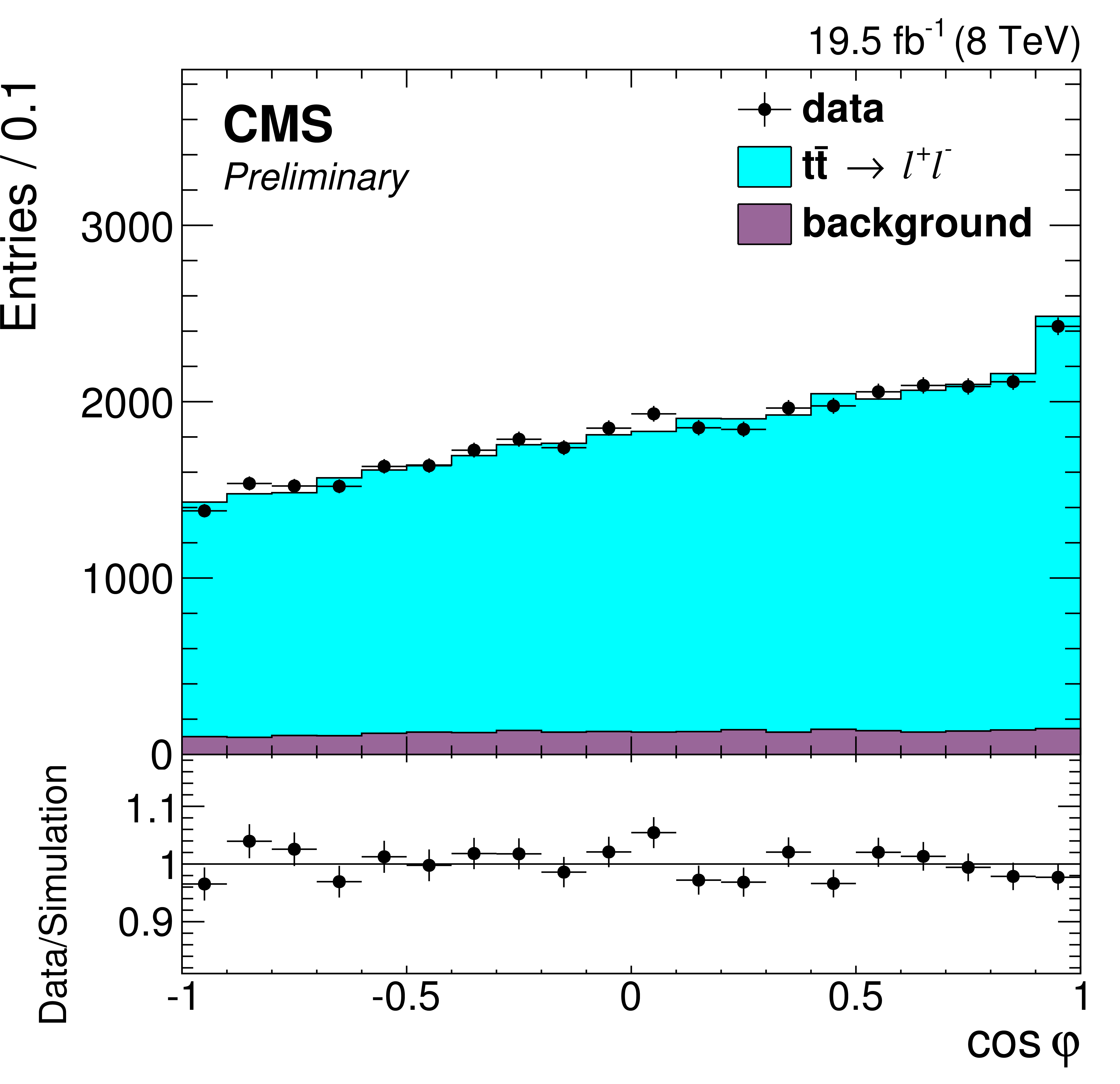
Figure 2-c:
The reconstructed angular distributions from data (points) and simulation (histogram). All the dilepton flavour combinations are included. The signal yield is normalized to the background-subtracted data. The error bars on the data points represent the statistical uncertainties. |
png ; pdf |
Figure 2-d:
The reconstructed angular distributions from data (points) and simulation (histogram). All the dilepton flavour combinations are included. The signal yield is normalized to the background-subtracted data. The error bars on the data points represent the statistical uncertainties. |
png ; pdf |
Figure 2-e:
The reconstructed angular distributions from data (points) and simulation (histogram). All the dilepton flavour combinations are included. The signal yield is normalized to the background-subtracted data. The error bars on the data points represent the statistical uncertainties. |
png ; pdf |
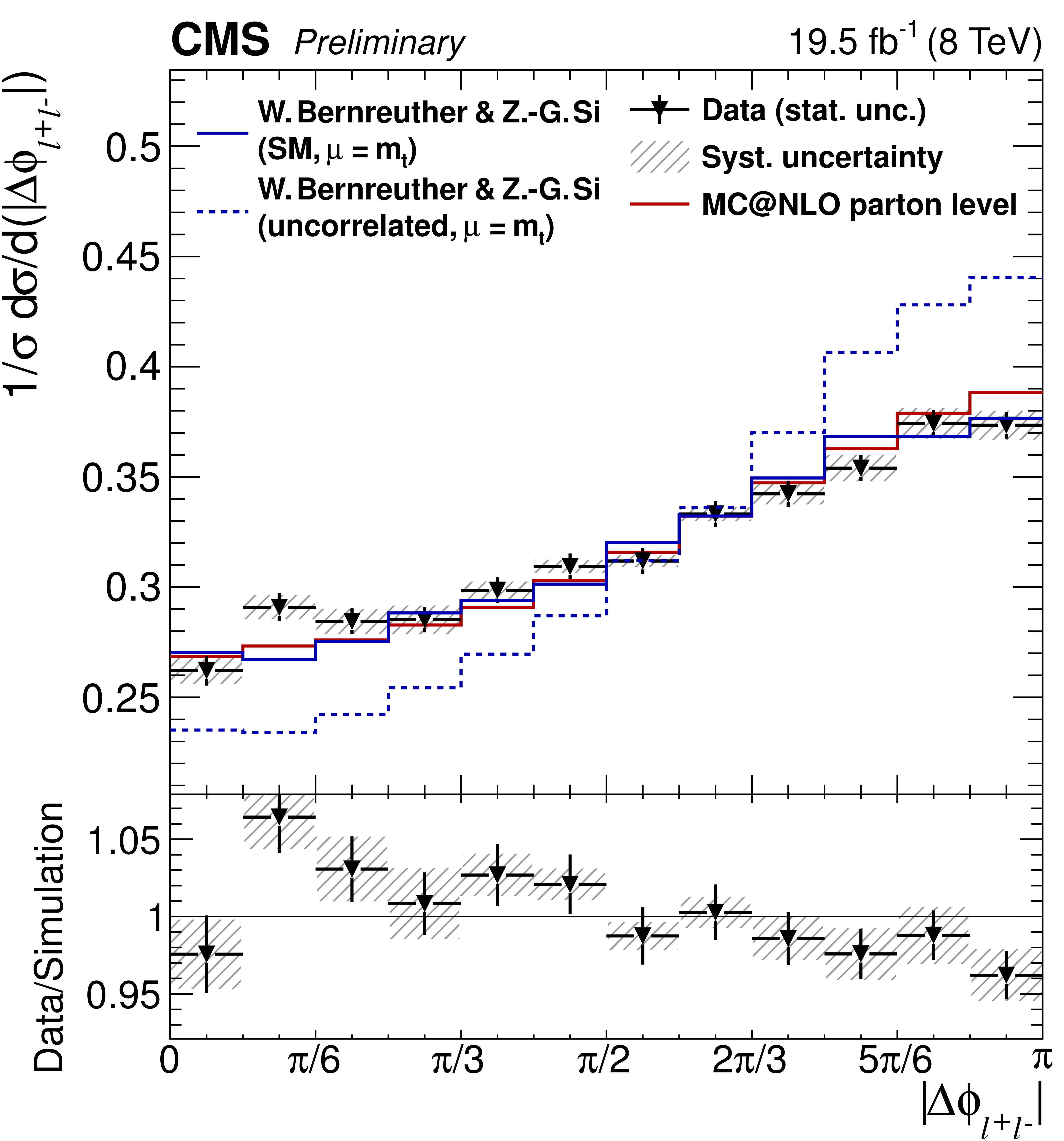
Figure 3-a:
Background-subtracted and unfolded differential measurements of $\left |\Delta \phi _{\ell ^+\ell ^-}\right |$, $\cos \theta^{\star }_\ell $, $c_{1} c_{2}$, and $\cos \varphi $, normalized to unit area (points), parton-level predictions from mc@nlo (red histograms), and theoretical predictions at NLO+EW (blue histograms). For the $\cos \theta ^{\star }_\ell $ distribution, CP conservation is assumed in the combination of measurements from positively and negatively charged leptons. The ratio of the measured bins with the mc@nlo prediction is shown in the bottom panel, and their statistical and systematic uncertainties are represented by the error bars and the hatched band, respectively. |
png ; pdf |
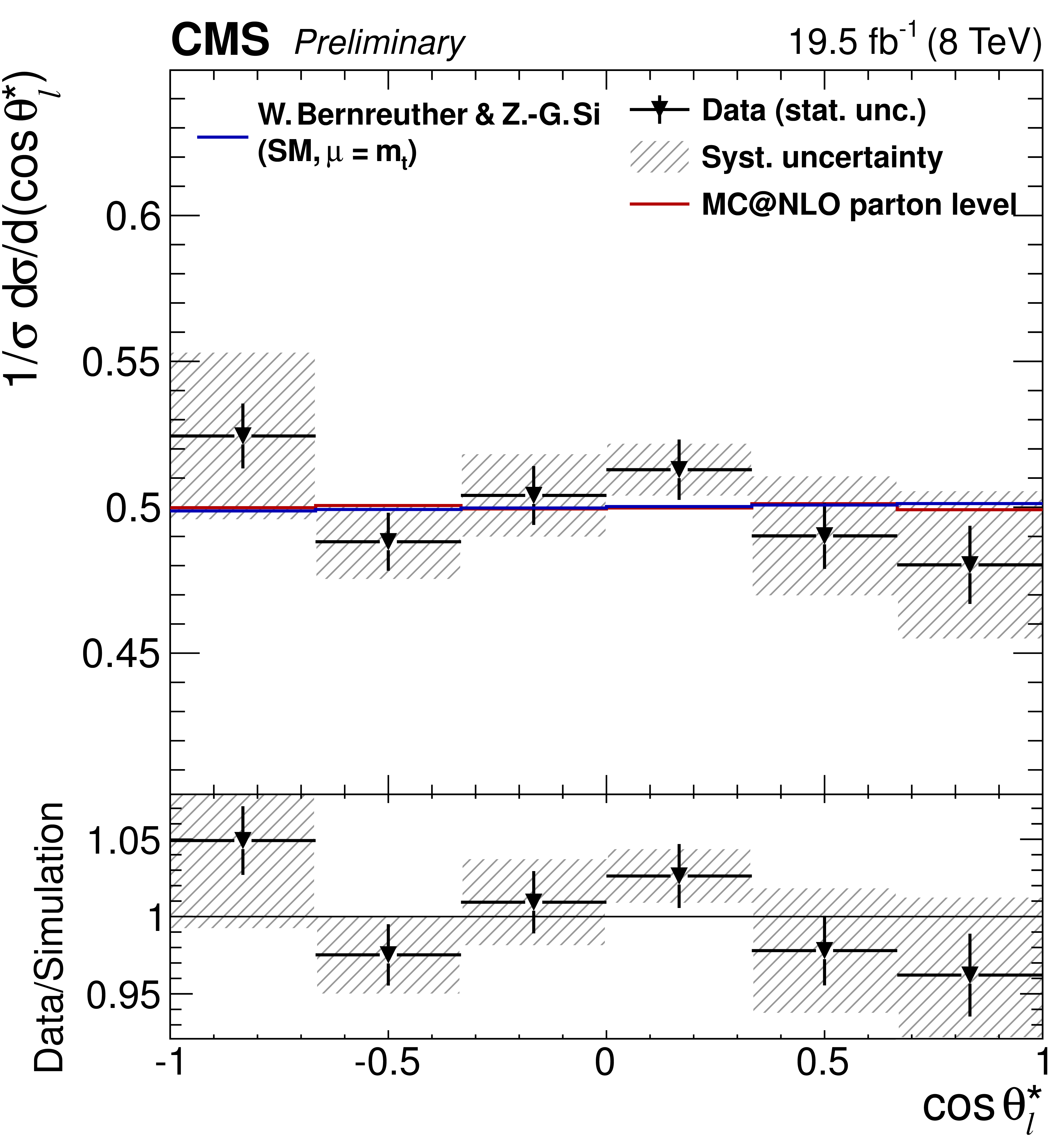
Figure 3-b:
Background-subtracted and unfolded differential measurements of $\left |\Delta \phi _{\ell ^+\ell ^-}\right |$, $\cos \theta^{\star }_\ell $, $c_{1} c_{2}$, and $\cos \varphi $, normalized to unit area (points), parton-level predictions from mc@nlo (red histograms), and theoretical predictions at NLO+EW (blue histograms). For the $\cos \theta ^{\star }_\ell $ distribution, CP conservation is assumed in the combination of measurements from positively and negatively charged leptons. The ratio of the measured bins with the mc@nlo prediction is shown in the bottom panel, and their statistical and systematic uncertainties are represented by the error bars and the hatched band, respectively. |
png ; pdf |
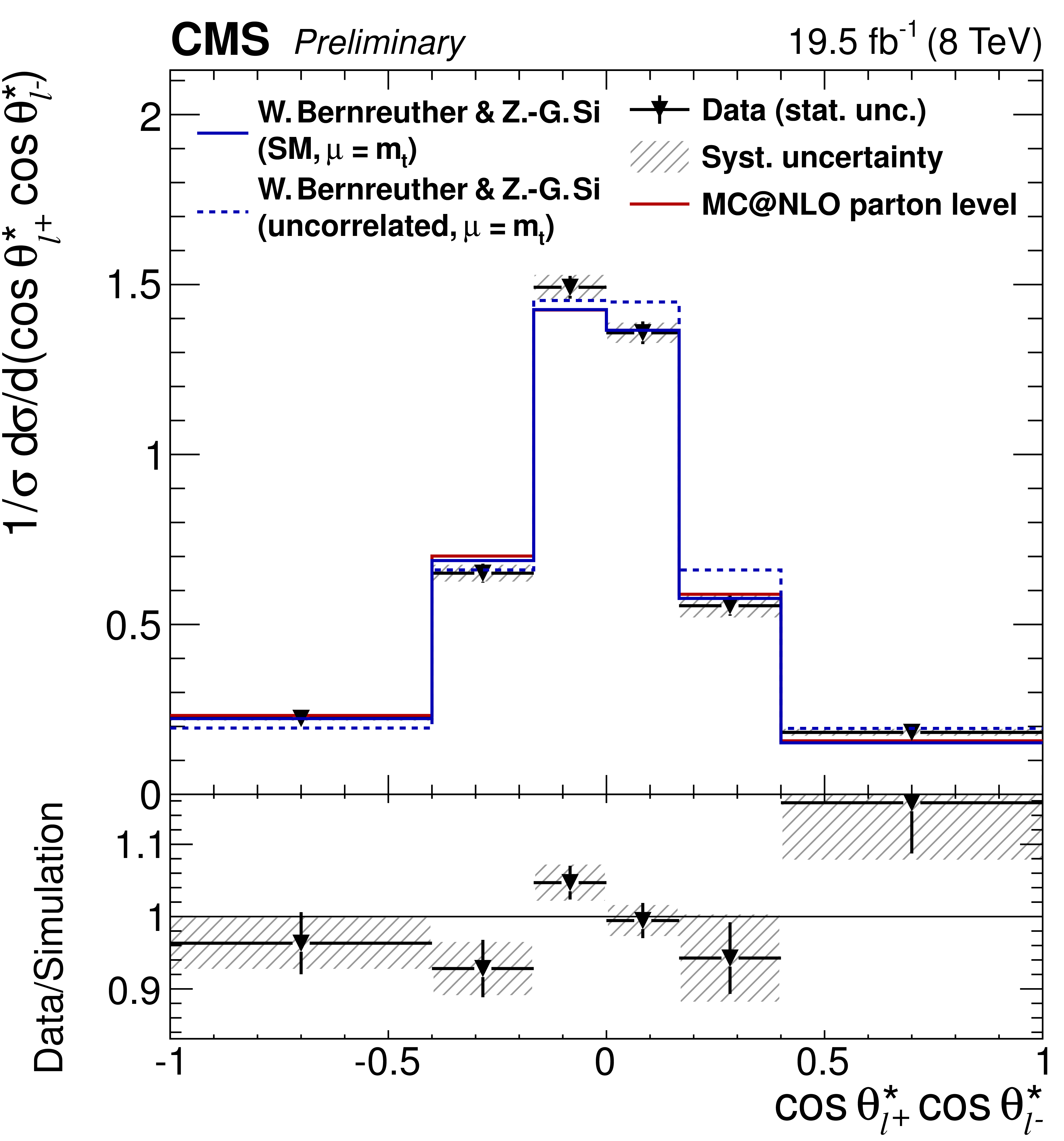
Figure 3-c:
Background-subtracted and unfolded differential measurements of $\left |\Delta \phi _{\ell ^+\ell ^-}\right |$, $\cos \theta^{\star }_\ell $, $c_{1} c_{2}$, and $\cos \varphi $, normalized to unit area (points), parton-level predictions from mc@nlo (red histograms), and theoretical predictions at NLO+EW (blue histograms). For the $\cos \theta ^{\star }_\ell $ distribution, CP conservation is assumed in the combination of measurements from positively and negatively charged leptons. The ratio of the measured bins with the mc@nlo prediction is shown in the bottom panel, and their statistical and systematic uncertainties are represented by the error bars and the hatched band, respectively. |

png ; pdf |
Figure 3-d:
Background-subtracted and unfolded differential measurements of $\left |\Delta \phi _{\ell ^+\ell ^-}\right |$, $\cos \theta^{\star }_\ell $, $c_{1} c_{2}$, and $\cos \varphi $, normalized to unit area (points), parton-level predictions from mc@nlo (red histograms), and theoretical predictions at NLO+EW (blue histograms). For the $\cos \theta ^{\star }_\ell $ distribution, CP conservation is assumed in the combination of measurements from positively and negatively charged leptons. The ratio of the measured bins with the mc@nlo prediction is shown in the bottom panel, and their statistical and systematic uncertainties are represented by the error bars and the hatched band, respectively. |
png ; pdf |
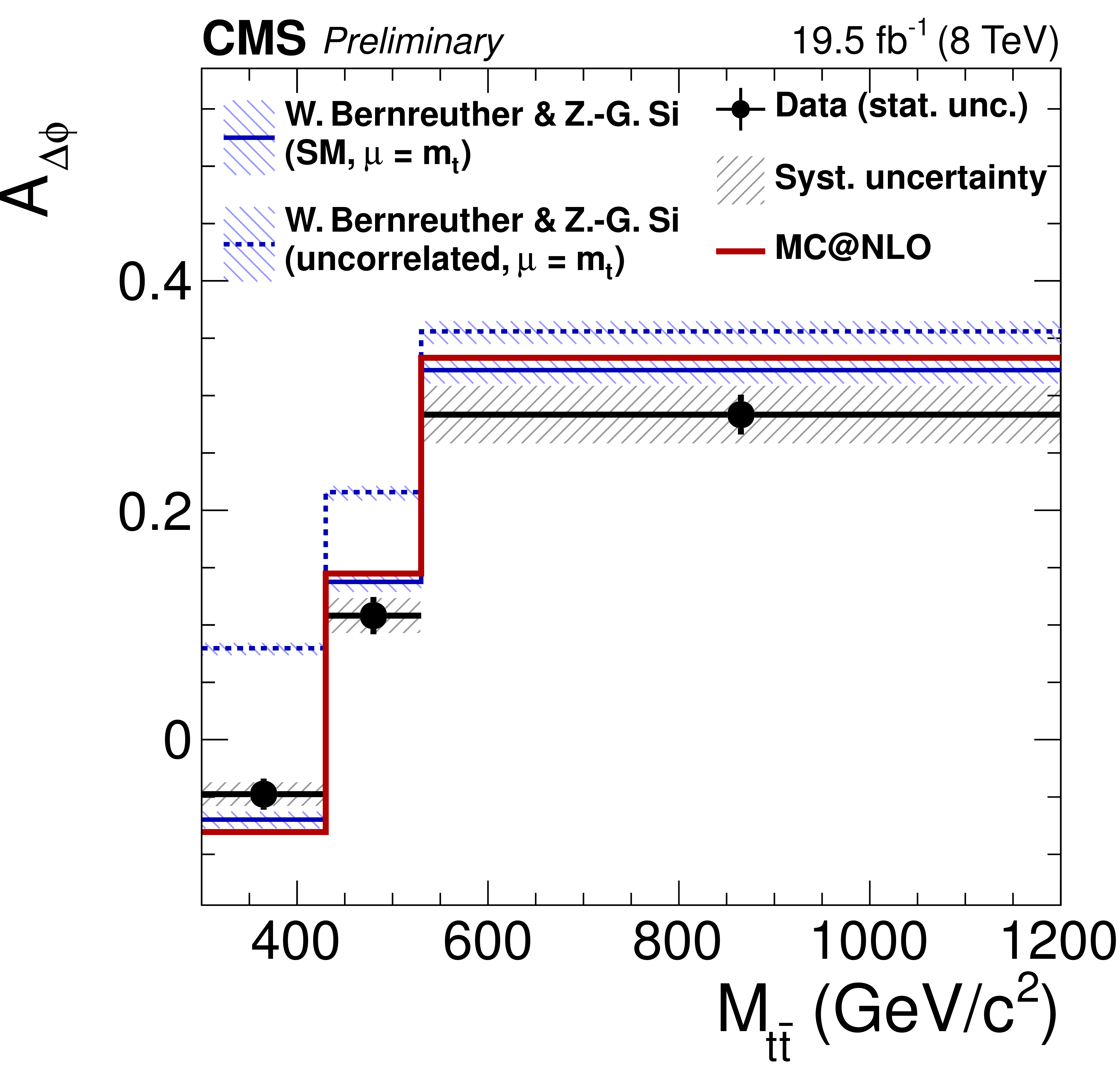
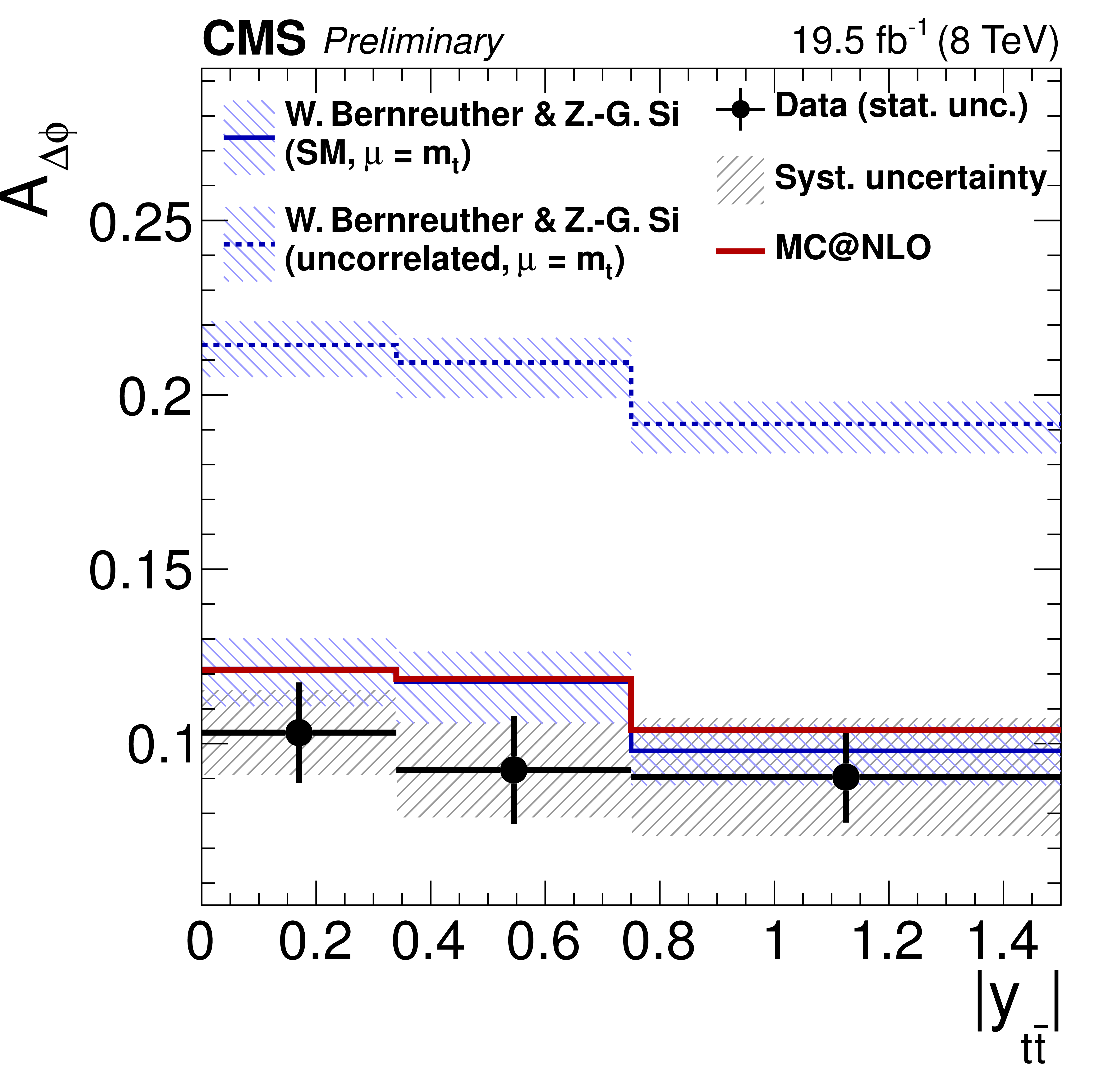
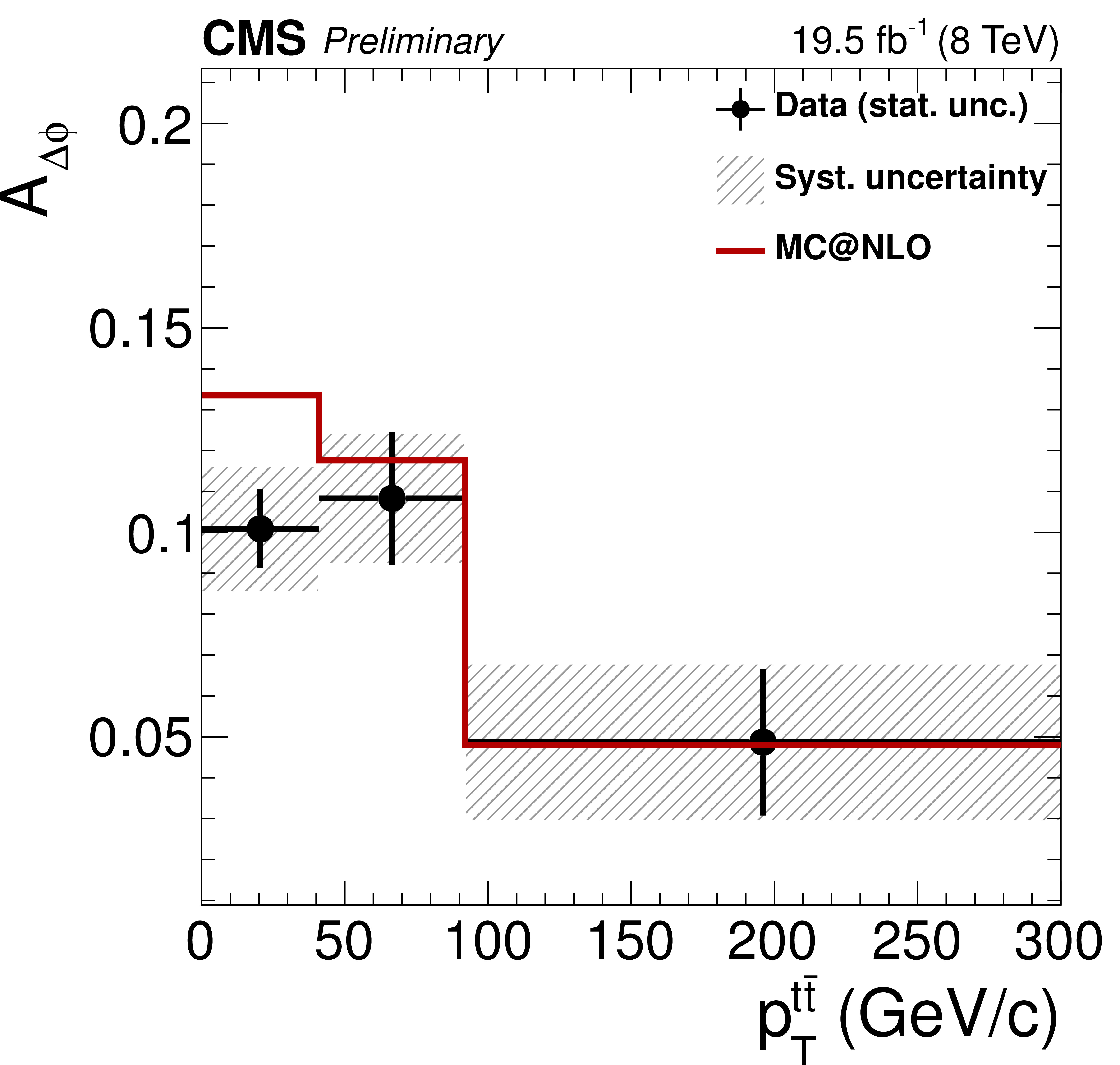
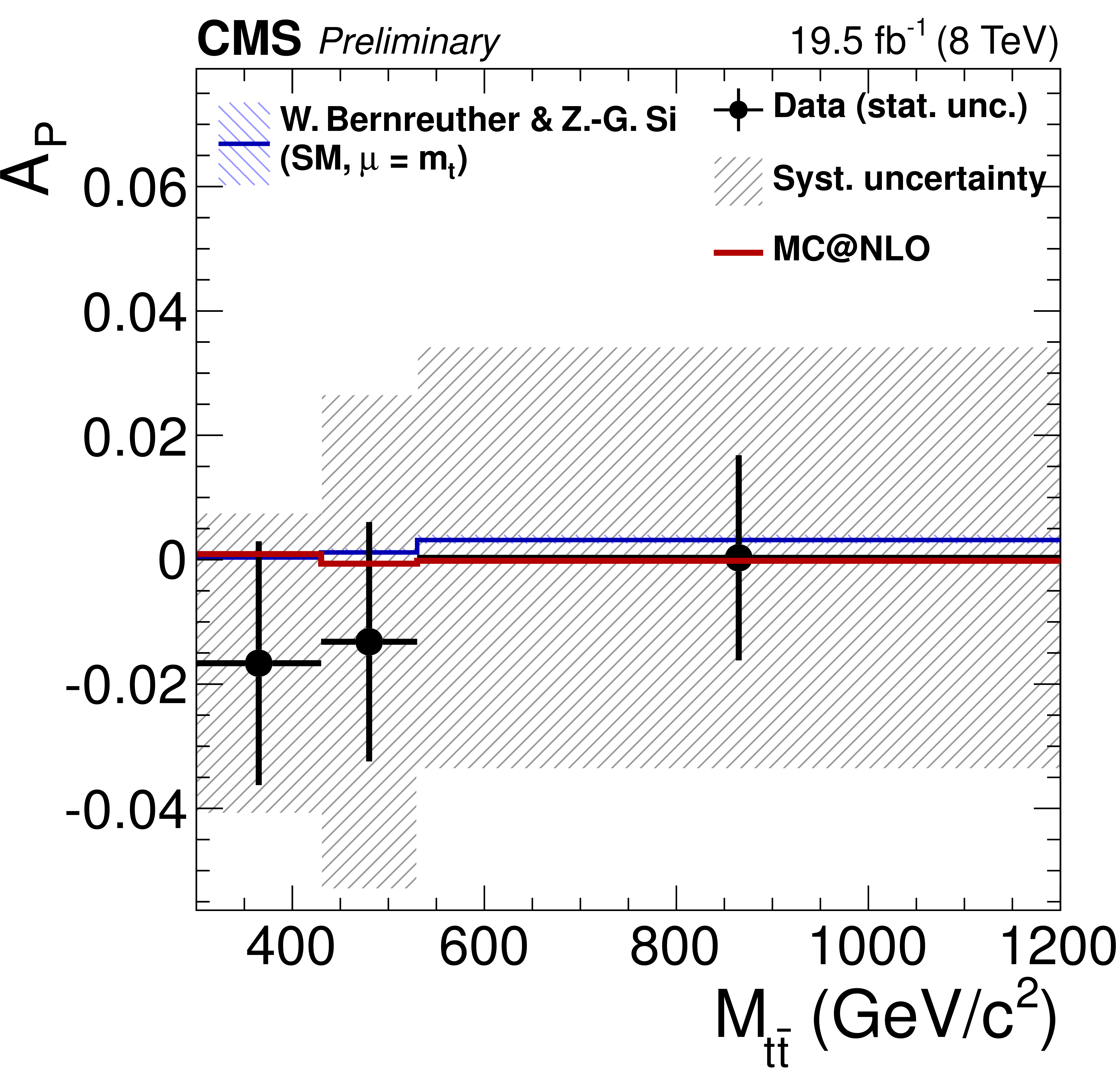
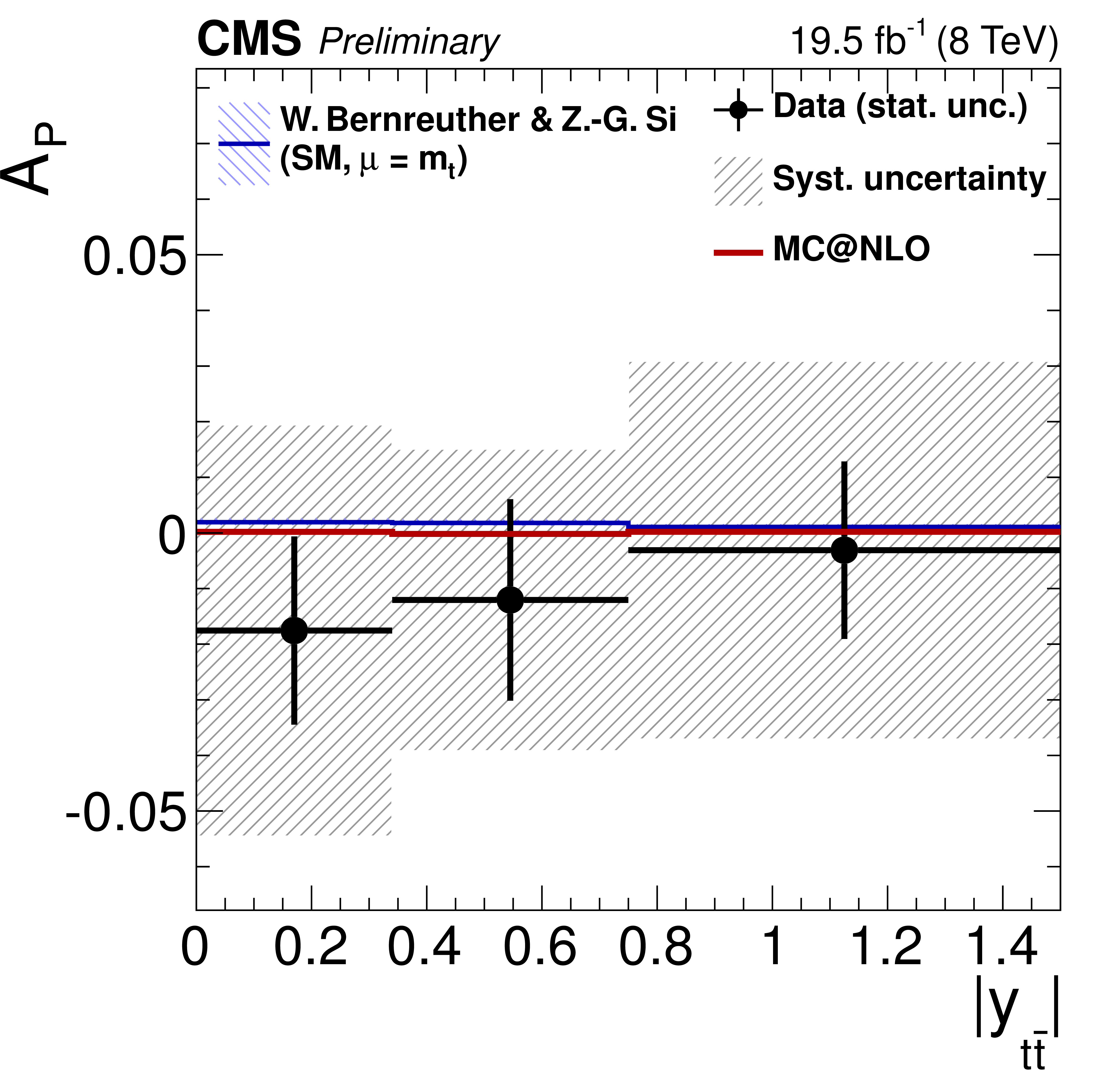
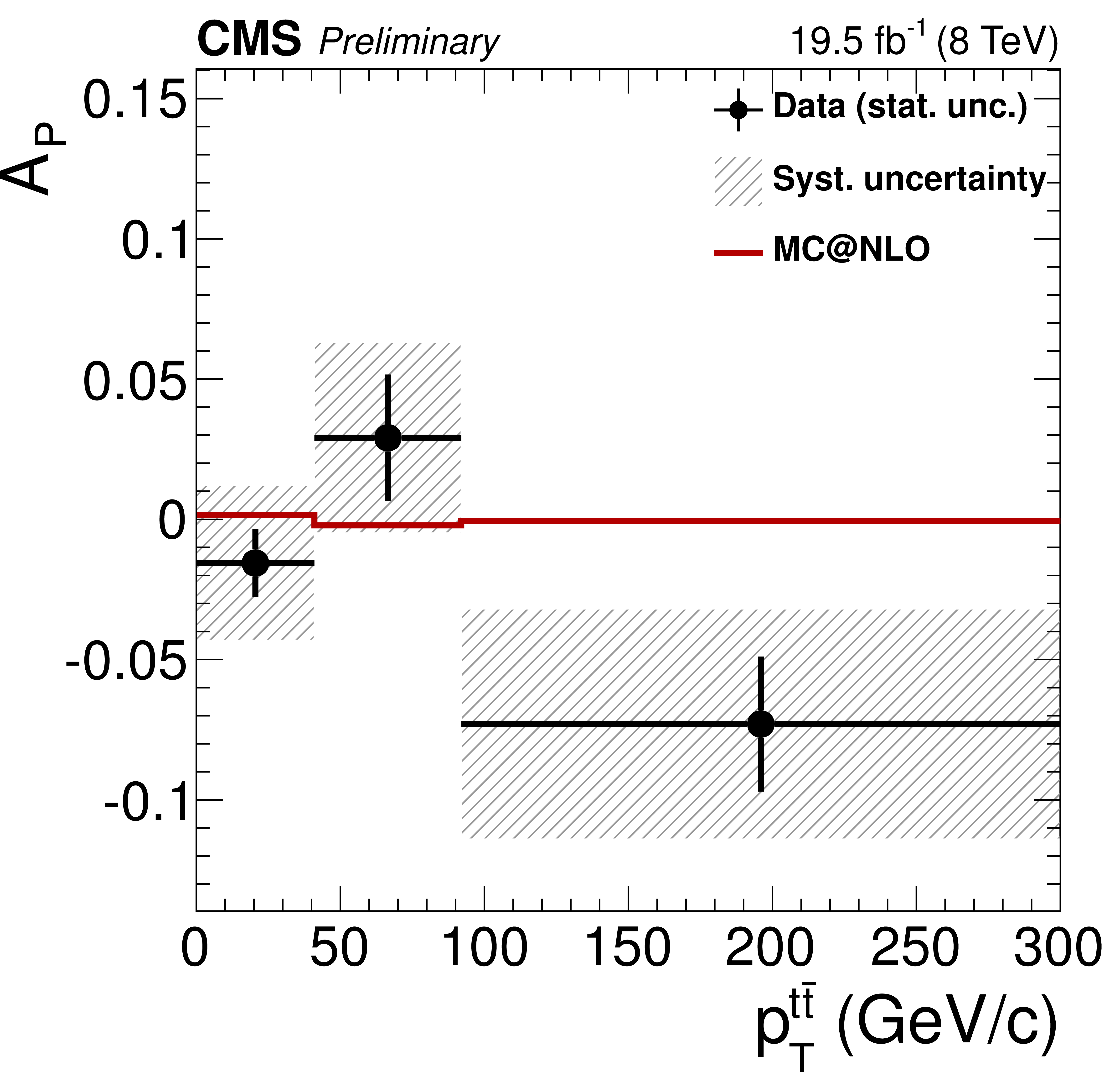
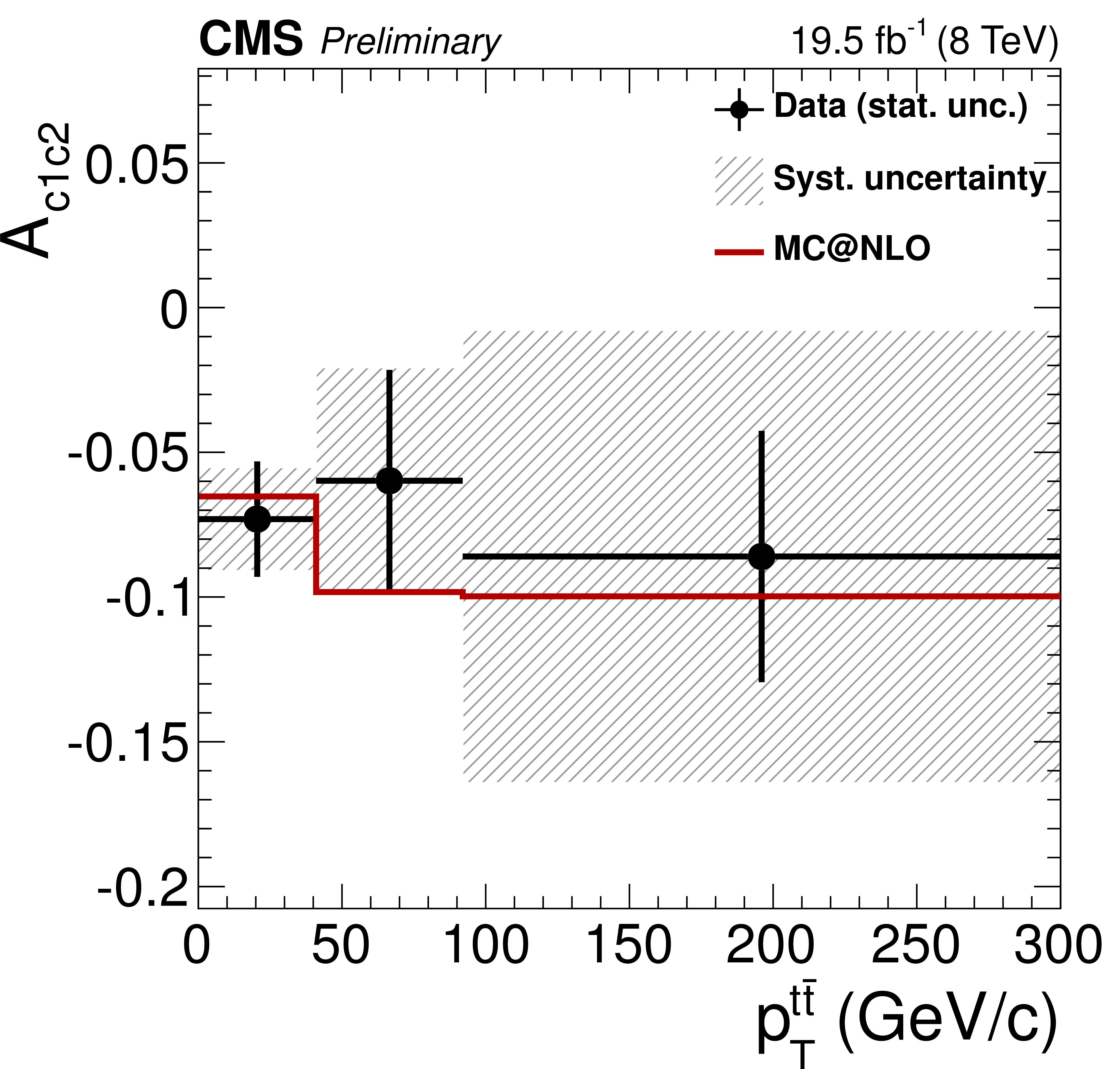
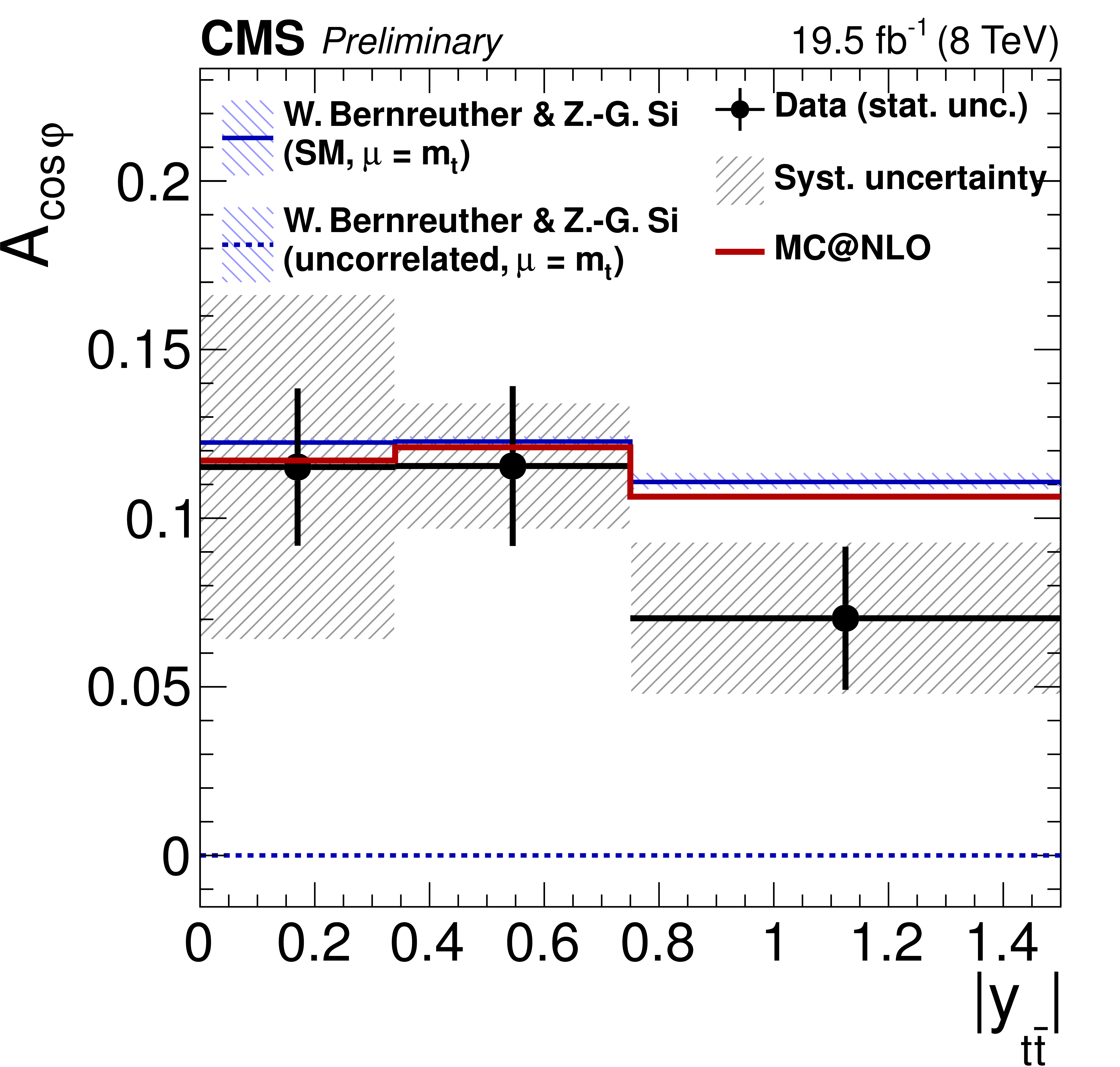
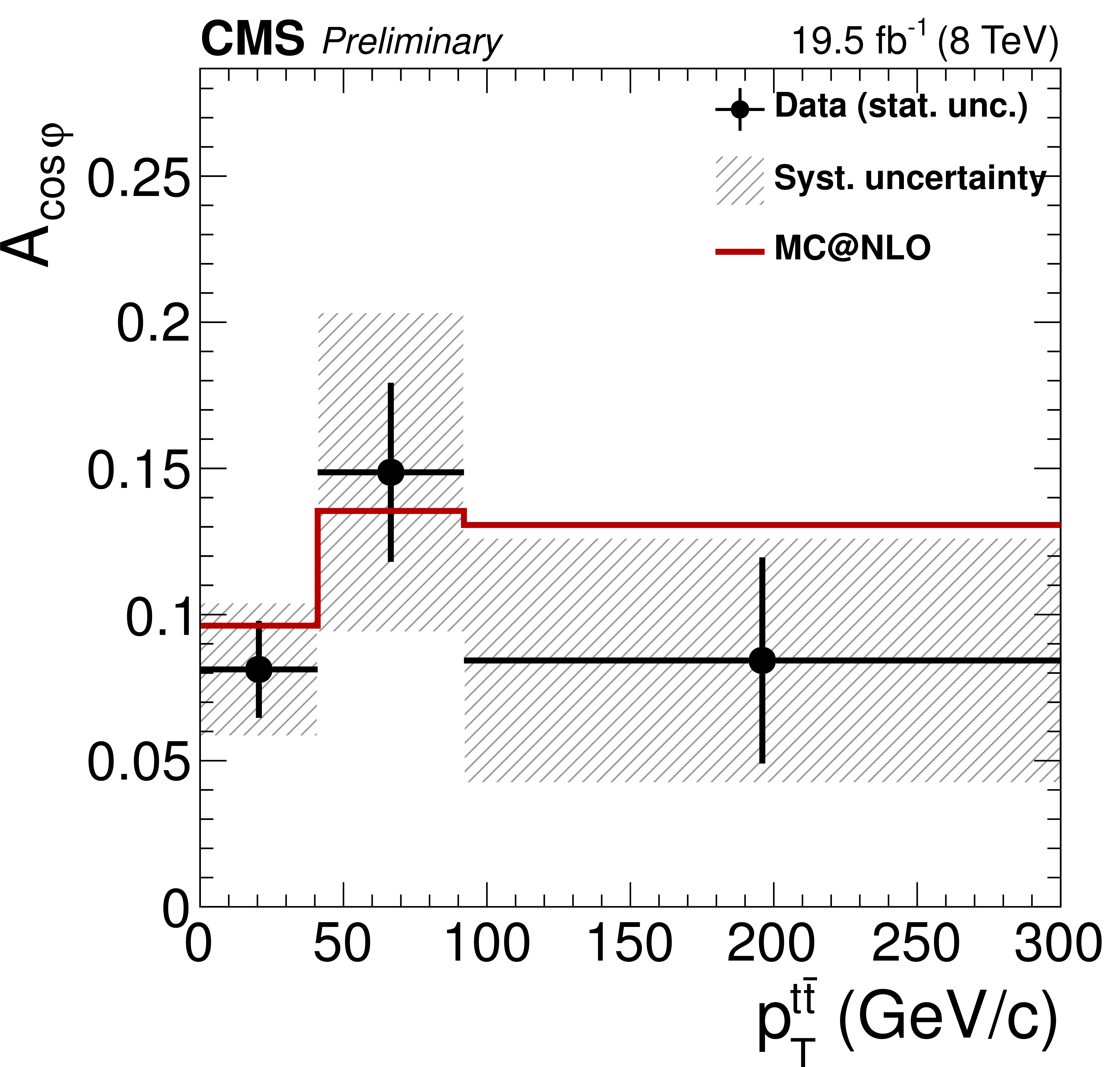
Figure 4-a:
Dependence of the asymmetry variables obtained from the unfolded distributions (points) on $M_{ {\mathrm {t}\overline {\mathrm {t}}} }$ (a,d,g,j), $ {| y_{ {\mathrm {t}\overline {\mathrm {t}}} } | }$ (b,e,h,k), and $ {p_{\mathrm {T}}} ^{ {\mathrm {t}\overline {\mathrm {t}}} }$ (c,f,i,l), parton-level predictions from mc@nlo (red histograms), and theoretical predictions at NLO+EW (blue histograms). The statistical and systematic uncertainties of the measured bins are represented by the error bars and the grey hatched band, respectively. The theoretical factorization and renormalization scale uncertainties are represented by the pale blue hatched band. The last bin of each plot includes overflow events. |
png ; pdf |
Figure 4-b:
Dependence of the asymmetry variables obtained from the unfolded distributions (points) on $M_{ {\mathrm {t}\overline {\mathrm {t}}} }$ (a,d,g,j), $ {| y_{ {\mathrm {t}\overline {\mathrm {t}}} } | }$ (b,e,h,k), and $ {p_{\mathrm {T}}} ^{ {\mathrm {t}\overline {\mathrm {t}}} }$ (c,f,i,l), parton-level predictions from mc@nlo (red histograms), and theoretical predictions at NLO+EW (blue histograms). The statistical and systematic uncertainties of the measured bins are represented by the error bars and the grey hatched band, respectively. The theoretical factorization and renormalization scale uncertainties are represented by the pale blue hatched band. The last bin of each plot includes overflow events. |
png ; pdf |
Figure 4-c:
Dependence of the asymmetry variables obtained from the unfolded distributions (points) on $M_{ {\mathrm {t}\overline {\mathrm {t}}} }$ (a,d,g,j), $ {| y_{ {\mathrm {t}\overline {\mathrm {t}}} } | }$ (b,e,h,k), and $ {p_{\mathrm {T}}} ^{ {\mathrm {t}\overline {\mathrm {t}}} }$ (c,f,i,l), parton-level predictions from mc@nlo (red histograms), and theoretical predictions at NLO+EW (blue histograms). The statistical and systematic uncertainties of the measured bins are represented by the error bars and the grey hatched band, respectively. The theoretical factorization and renormalization scale uncertainties are represented by the pale blue hatched band. The last bin of each plot includes overflow events. |
png ; pdf |
Figure 4-d:
Dependence of the asymmetry variables obtained from the unfolded distributions (points) on $M_{ {\mathrm {t}\overline {\mathrm {t}}} }$ (a,d,g,j), $ {| y_{ {\mathrm {t}\overline {\mathrm {t}}} } | }$ (b,e,h,k), and $ {p_{\mathrm {T}}} ^{ {\mathrm {t}\overline {\mathrm {t}}} }$ (c,f,i,l), parton-level predictions from mc@nlo (red histograms), and theoretical predictions at NLO+EW (blue histograms). The statistical and systematic uncertainties of the measured bins are represented by the error bars and the grey hatched band, respectively. The theoretical factorization and renormalization scale uncertainties are represented by the pale blue hatched band. The last bin of each plot includes overflow events. |
png ; pdf |
Figure 4-e:
Dependence of the asymmetry variables obtained from the unfolded distributions (points) on $M_{ {\mathrm {t}\overline {\mathrm {t}}} }$ (a,d,g,j), $ {| y_{ {\mathrm {t}\overline {\mathrm {t}}} } | }$ (b,e,h,k), and $ {p_{\mathrm {T}}} ^{ {\mathrm {t}\overline {\mathrm {t}}} }$ (c,f,i,l), parton-level predictions from mc@nlo (red histograms), and theoretical predictions at NLO+EW (blue histograms). The statistical and systematic uncertainties of the measured bins are represented by the error bars and the grey hatched band, respectively. The theoretical factorization and renormalization scale uncertainties are represented by the pale blue hatched band. The last bin of each plot includes overflow events. |
png ; pdf |
Figure 4-f:
Dependence of the asymmetry variables obtained from the unfolded distributions (points) on $M_{ {\mathrm {t}\overline {\mathrm {t}}} }$ (a,d,g,j), $ {| y_{ {\mathrm {t}\overline {\mathrm {t}}} } | }$ (b,e,h,k), and $ {p_{\mathrm {T}}} ^{ {\mathrm {t}\overline {\mathrm {t}}} }$ (c,f,i,l), parton-level predictions from mc@nlo (red histograms), and theoretical predictions at NLO+EW (blue histograms). The statistical and systematic uncertainties of the measured bins are represented by the error bars and the grey hatched band, respectively. The theoretical factorization and renormalization scale uncertainties are represented by the pale blue hatched band. The last bin of each plot includes overflow events. |

png ; pdf |
Figure 4-g:
Dependence of the asymmetry variables obtained from the unfolded distributions (points) on $M_{ {\mathrm {t}\overline {\mathrm {t}}} }$ (a,d,g,j), $ {| y_{ {\mathrm {t}\overline {\mathrm {t}}} } | }$ (b,e,h,k), and $ {p_{\mathrm {T}}} ^{ {\mathrm {t}\overline {\mathrm {t}}} }$ (c,f,i,l), parton-level predictions from mc@nlo (red histograms), and theoretical predictions at NLO+EW (blue histograms). The statistical and systematic uncertainties of the measured bins are represented by the error bars and the grey hatched band, respectively. The theoretical factorization and renormalization scale uncertainties are represented by the pale blue hatched band. The last bin of each plot includes overflow events. |

png ; pdf |
Figure 4-h:
Dependence of the asymmetry variables obtained from the unfolded distributions (points) on $M_{ {\mathrm {t}\overline {\mathrm {t}}} }$ (a,d,g,j), $ {| y_{ {\mathrm {t}\overline {\mathrm {t}}} } | }$ (b,e,h,k), and $ {p_{\mathrm {T}}} ^{ {\mathrm {t}\overline {\mathrm {t}}} }$ (c,f,i,l), parton-level predictions from mc@nlo (red histograms), and theoretical predictions at NLO+EW (blue histograms). The statistical and systematic uncertainties of the measured bins are represented by the error bars and the grey hatched band, respectively. The theoretical factorization and renormalization scale uncertainties are represented by the pale blue hatched band. The last bin of each plot includes overflow events. |
png ; pdf |
Figure 4-i:
Dependence of the asymmetry variables obtained from the unfolded distributions (points) on $M_{ {\mathrm {t}\overline {\mathrm {t}}} }$ (a,d,g,j), $ {| y_{ {\mathrm {t}\overline {\mathrm {t}}} } | }$ (b,e,h,k), and $ {p_{\mathrm {T}}} ^{ {\mathrm {t}\overline {\mathrm {t}}} }$ (c,f,i,l), parton-level predictions from mc@nlo (red histograms), and theoretical predictions at NLO+EW (blue histograms). The statistical and systematic uncertainties of the measured bins are represented by the error bars and the grey hatched band, respectively. The theoretical factorization and renormalization scale uncertainties are represented by the pale blue hatched band. The last bin of each plot includes overflow events. |

png ; pdf |
Figure 4-j:
Dependence of the asymmetry variables obtained from the unfolded distributions (points) on $M_{ {\mathrm {t}\overline {\mathrm {t}}} }$ (a,d,g,j), $ {| y_{ {\mathrm {t}\overline {\mathrm {t}}} } | }$ (b,e,h,k), and $ {p_{\mathrm {T}}} ^{ {\mathrm {t}\overline {\mathrm {t}}} }$ (c,f,i,l), parton-level predictions from mc@nlo (red histograms), and theoretical predictions at NLO+EW (blue histograms). The statistical and systematic uncertainties of the measured bins are represented by the error bars and the grey hatched band, respectively. The theoretical factorization and renormalization scale uncertainties are represented by the pale blue hatched band. The last bin of each plot includes overflow events. |
png ; pdf |
Figure 4-k:
Dependence of the asymmetry variables obtained from the unfolded distributions (points) on $M_{ {\mathrm {t}\overline {\mathrm {t}}} }$ (a,d,g,j), $ {| y_{ {\mathrm {t}\overline {\mathrm {t}}} } | }$ (b,e,h,k), and $ {p_{\mathrm {T}}} ^{ {\mathrm {t}\overline {\mathrm {t}}} }$ (c,f,i,l), parton-level predictions from mc@nlo (red histograms), and theoretical predictions at NLO+EW (blue histograms). The statistical and systematic uncertainties of the measured bins are represented by the error bars and the grey hatched band, respectively. The theoretical factorization and renormalization scale uncertainties are represented by the pale blue hatched band. The last bin of each plot includes overflow events. |
png ; pdf |
Figure 4-l:
Dependence of the asymmetry variables obtained from the unfolded distributions (points) on $M_{ {\mathrm {t}\overline {\mathrm {t}}} }$ (a,d,g,j), $ {| y_{ {\mathrm {t}\overline {\mathrm {t}}} } | }$ (b,e,h,k), and $ {p_{\mathrm {T}}} ^{ {\mathrm {t}\overline {\mathrm {t}}} }$ (c,f,i,l), parton-level predictions from mc@nlo (red histograms), and theoretical predictions at NLO+EW (blue histograms). The statistical and systematic uncertainties of the measured bins are represented by the error bars and the grey hatched band, respectively. The theoretical factorization and renormalization scale uncertainties are represented by the pale blue hatched band. The last bin of each plot includes overflow events. |
png ; pdf |
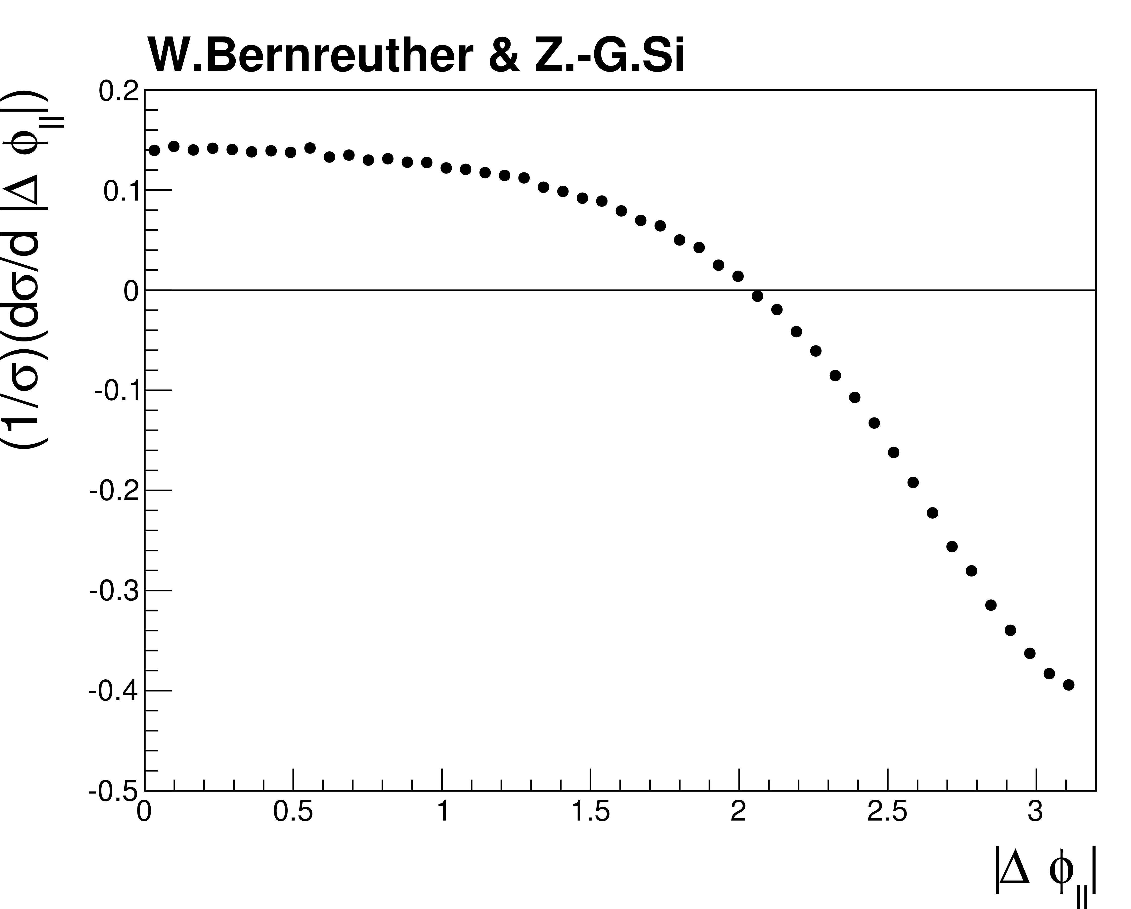
Figure 5:
Contribution from new physics with a non-zero CMDM to $(1/\sigma )(d\sigma /d\left |\Delta \phi _{\ell ^+\ell ^-}\right |)$ at the LHC ($\sqrt {s}=$ 8 TeV), for $\mathrm{Re} (\hat{\mu }_t)=$ 1, from [4]. A negative cross section arises from a negative interference term with SM $ {\mathrm {t}\overline {\mathrm {t}}} $ production. |

png ; pdf |
Figure 6:
$(1/\sigma )(d\sigma /d\left |\Delta \phi _{\ell ^+\ell ^-}\right |)$ differential cross section. The red line corresponds to the result of the fit, and the blue lines show the SM NLO+EW predictions for renormalization and factorization scales of $m_t$, $2m_t$ and $m_t/2$. |
|
|
Compact Muon Solenoid LHC, CERN |
|

|

|

|

|

|