

Compact Muon Solenoid
LHC, CERN
| CMS-PAS-SUS-15-006 | ||
| Search for supersymmetry in events with one lepton in proton-proton collisions at $ \sqrt{s} = $ 13 TeV with the CMS experiment | ||
| CMS Collaboration | ||
| March 2016 | ||
| Abstract: A search for supersymmetry in events with a single electron or muon is performed on proton-proton collision data with the CMS experiment at a center-of-mass energy of 13 TeV, in a dataset corresponding to an integrated luminosity of 2.3 fb$^{-1}$. Several exclusive search regions are defined, based on the number of b-tagged jets, the scalar sum of all jet transverse momenta, and the scalar sum of the transverse missing momentum and transverse lepton momentum. The observed yields are compatible with predictions from standard model processes. The results are interpreted in two simplified models describing gluino pair production. In a model where each gluino decays to top quarks and a neutralino, gluinos with masses up to 1.575 TeV are excluded for neutralino masses below 600 GeV. In the second model, each gluino decays to two light quarks and an intermediate chargino, with the latter decaying to a W boson and a neutralino. Here, gluino masses below 1.4 TeV are excluded for neutralino masses below 725 GeV, assuming a chargino with mass midway between the gluino and neutralino mass. | ||
|
Links:
CDS record (PDF) ;
CADI line (restricted) ;
These preliminary results are superseded in this paper, PRD 95 (2017) 012011. The superseded preliminary plots can be found here. |
||
| Figures | |
png pdf |
Figure 1-a:
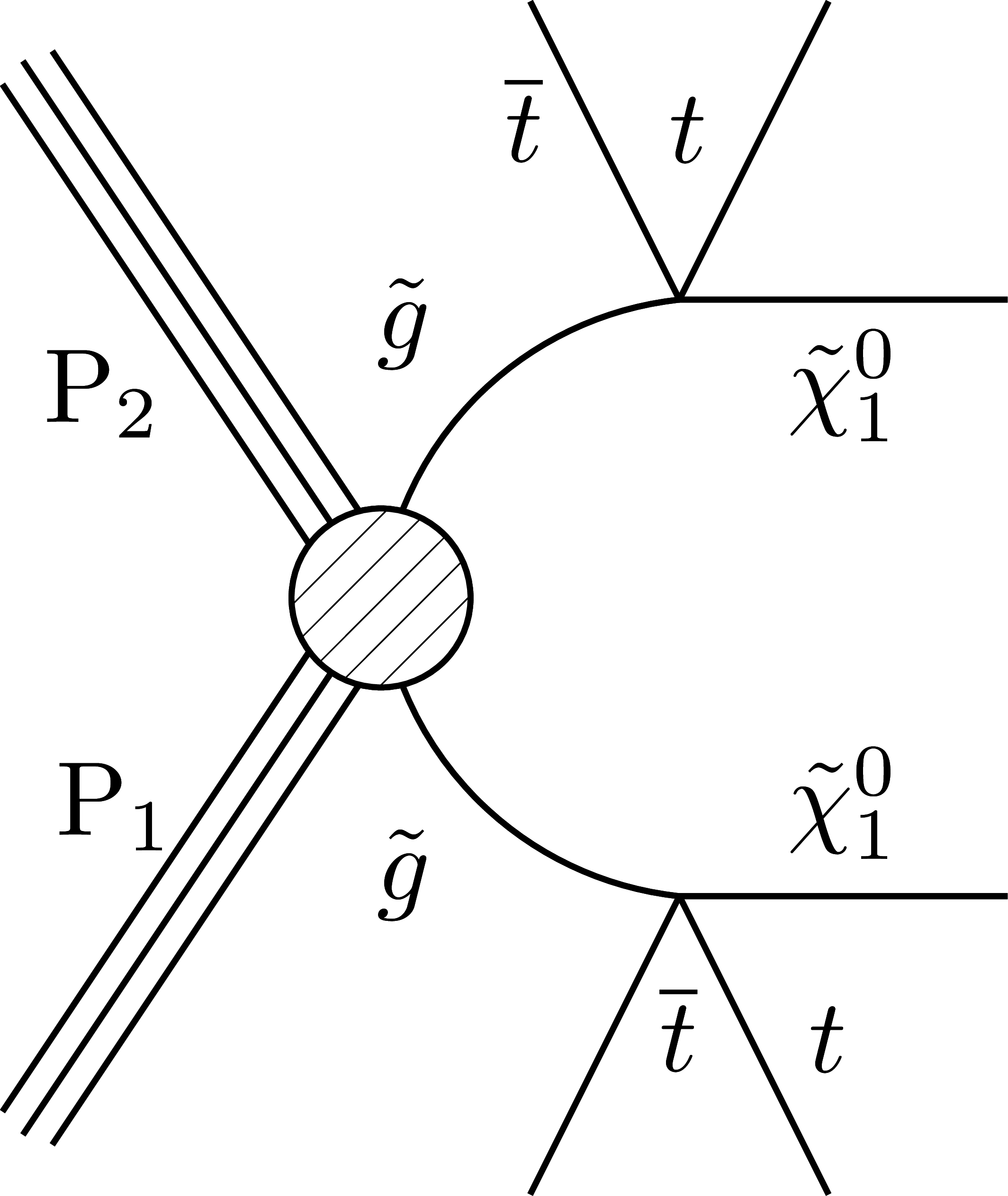
Graphs showing the simplified models T1t$^{4}$ (a) and T5q$^{4}$WW (b). Depending on the mass difference between the chargino ($ {\tilde{\chi}^{\pm }_1} $) and the neutralino ($ {\tilde{\chi}^0_1} $), the W boson can be virtual. |

png pdf |
Figure 1-b:
Graphs showing the simplified models T1t$^{4}$ (a) and T5q$^{4}$WW (b). Depending on the mass difference between the chargino ($ {\tilde{\chi}^{\pm }_1} $) and the neutralino ($ {\tilde{\chi}^0_1} $), the W boson can be virtual. |

png pdf |
Figure 2-a:
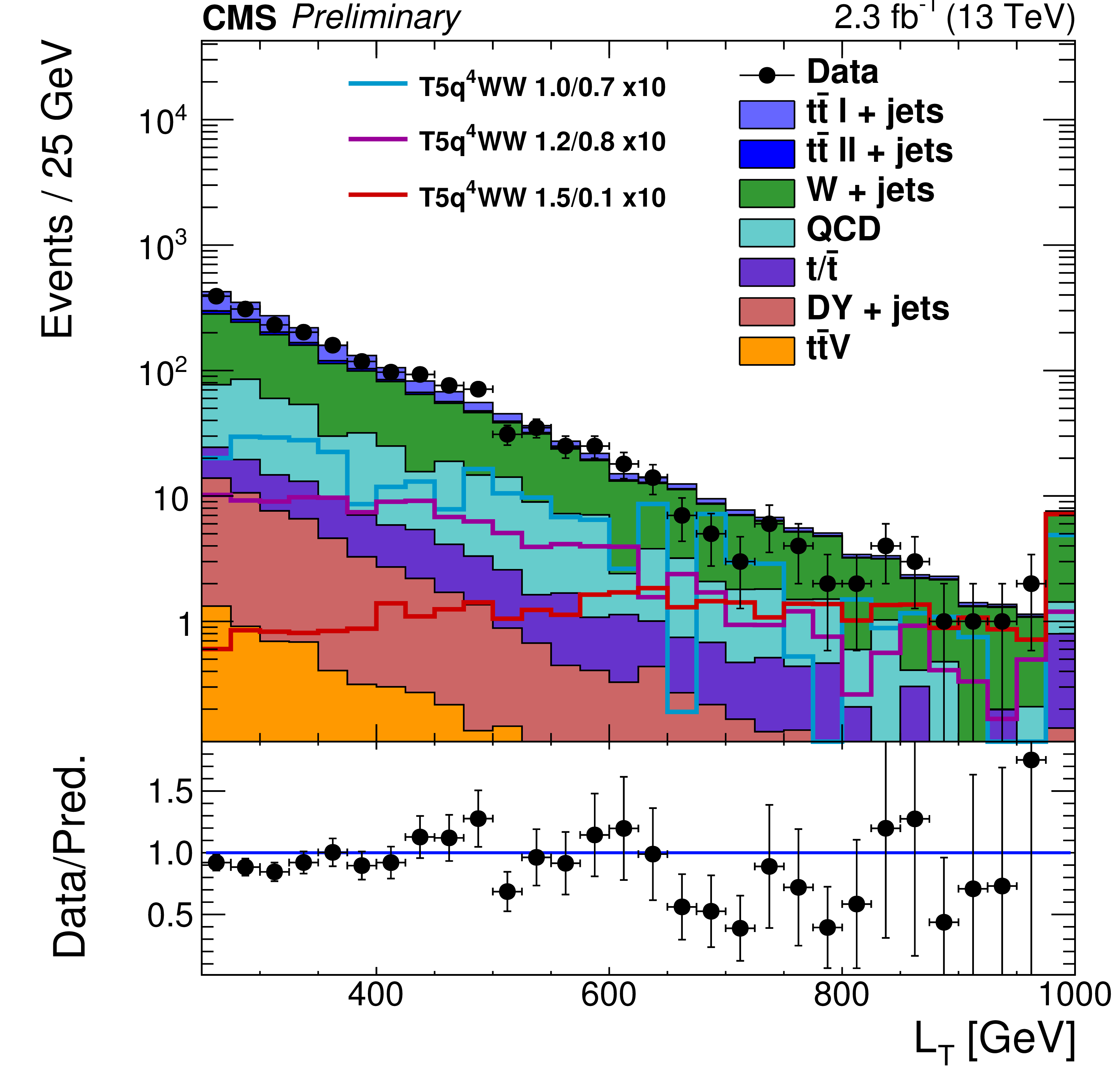
The $ {H_{\mathrm {T}}} $ distribution for the multi-b analysis in (a) and the $ {L_{\textrm T}} $ distribution for the zero-b analysis (b), both after the preselection, requiring at least six jets for the multi-b analysis, of which at least one is b-tagged, and at least five jets for the zero-b analysis, with no b-tagged jet. A minimum $ {H_{\mathrm {T}}} $ of 500 GeV and a minimum $ {L_{\textrm T}} $ of 250 GeV is required in addition to exactly one lepton with $ {p_{\mathrm {T}}} > $ 25 GeV. The simulated background events are stacked on top of each other, and several signal points are overlaid for illustration without being stacked. For the multi-b analysis, the model T1t$^{4}$ 1.2/0.8 (T1t$^{4}$ 1.5/0.1) corresponds to a gluino mass of 1.2 TeV (1.5 TeV) and neutralino mass of 0.8 TeV (0.1 TeV), respectively. For the zero-b analysis, the model T5q$^{4}$WW 1.0/0.7 (T5q$^{4}$WW 1.2/0.8 and T5q$^{4}$WW 1.5/0.1) corresponds to a gluino mass of 1.0 TeV (1.2 TeV and 1.5 TeV) and neutralino mass of 0.7 TeV (0.8 TeV and 0.1 TeV), respectively. For the latter, the intermediate chargino mass is fixed at 0.85 TeV (1.0 TeV and 0.8 TeV). |
png pdf |
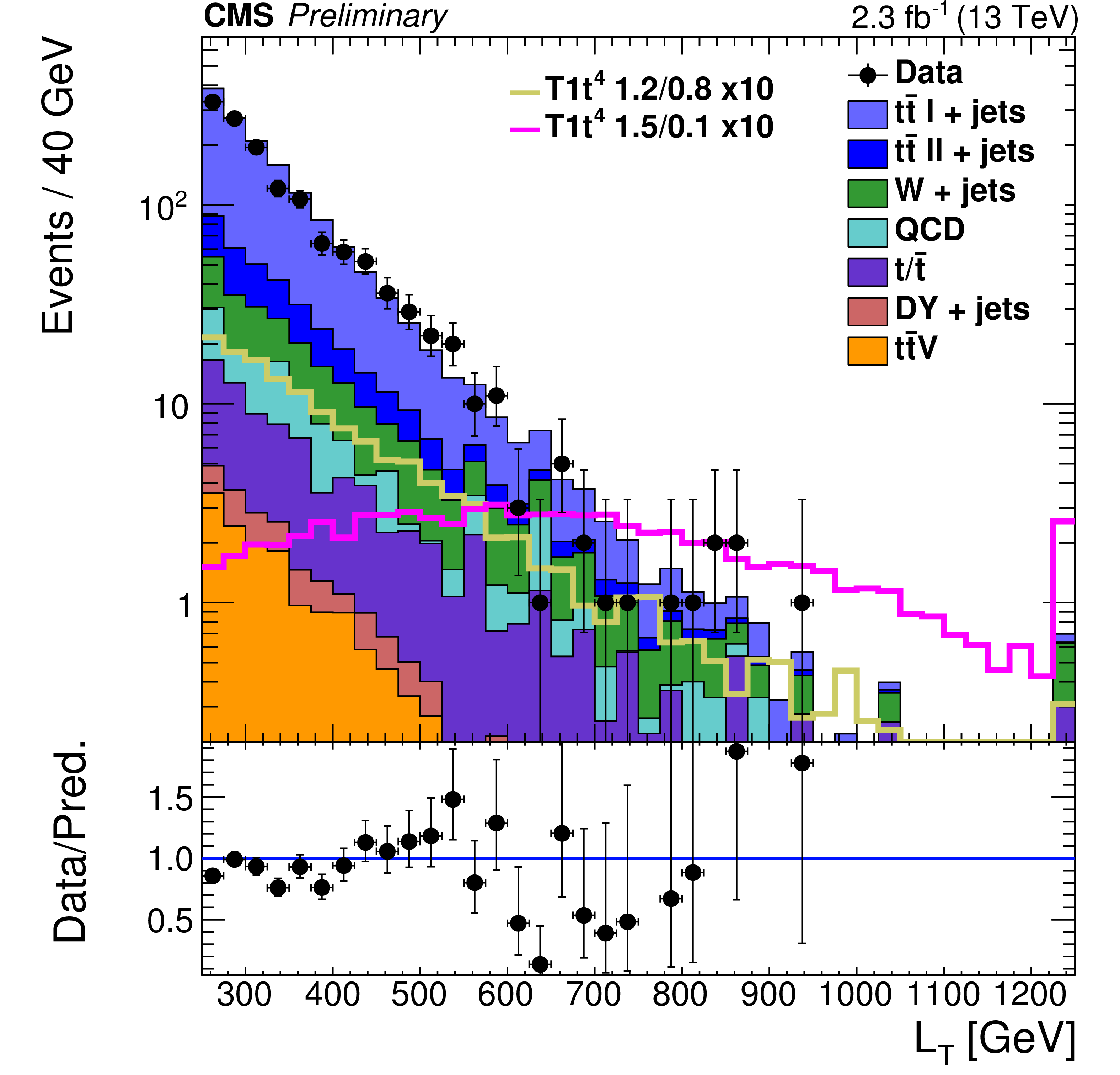
Figure 2-b:
The $ {H_{\mathrm {T}}} $ distribution for the multi-b analysis in (a) and the $ {L_{\textrm T}} $ distribution for the zero-b analysis (b), both after the preselection, requiring at least six jets for the multi-b analysis, of which at least one is b-tagged, and at least five jets for the zero-b analysis, with no b-tagged jet. A minimum $ {H_{\mathrm {T}}} $ of 500 GeV and a minimum $ {L_{\textrm T}} $ of 250 GeV is required in addition to exactly one lepton with $ {p_{\mathrm {T}}} > $ 25 GeV. The simulated background events are stacked on top of each other, and several signal points are overlaid for illustration without being stacked. For the multi-b analysis, the model T1t$^{4}$ 1.2/0.8 (T1t$^{4}$ 1.5/0.1) corresponds to a gluino mass of 1.2 TeV (1.5 TeV) and neutralino mass of 0.8 TeV (0.1 TeV), respectively. For the zero-b analysis, the model T5q$^{4}$WW 1.0/0.7 (T5q$^{4}$WW 1.2/0.8 and T5q$^{4}$WW 1.5/0.1) corresponds to a gluino mass of 1.0 TeV (1.2 TeV and 1.5 TeV) and neutralino mass of 0.7 TeV (0.8 TeV and 0.1 TeV), respectively. For the latter, the intermediate chargino mass is fixed at 0.85 TeV (1.0 TeV and 0.8 TeV). |

png pdf |
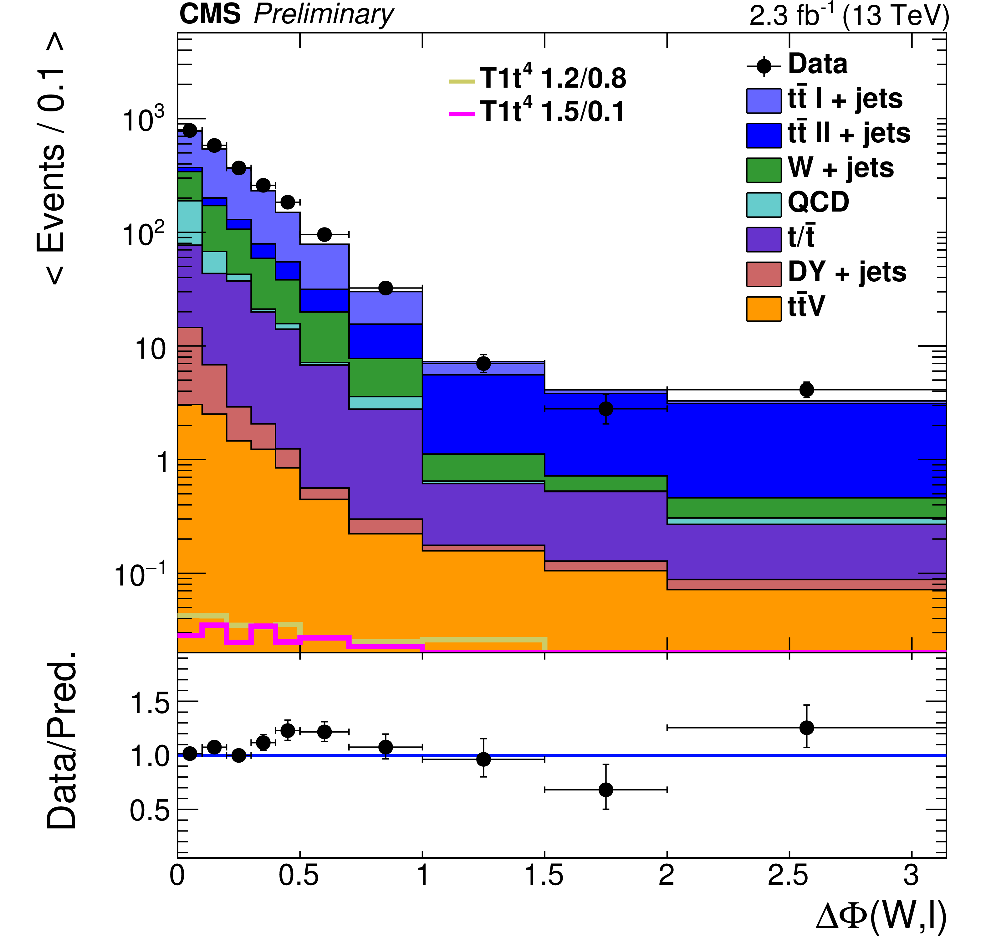
Figure 3-a:
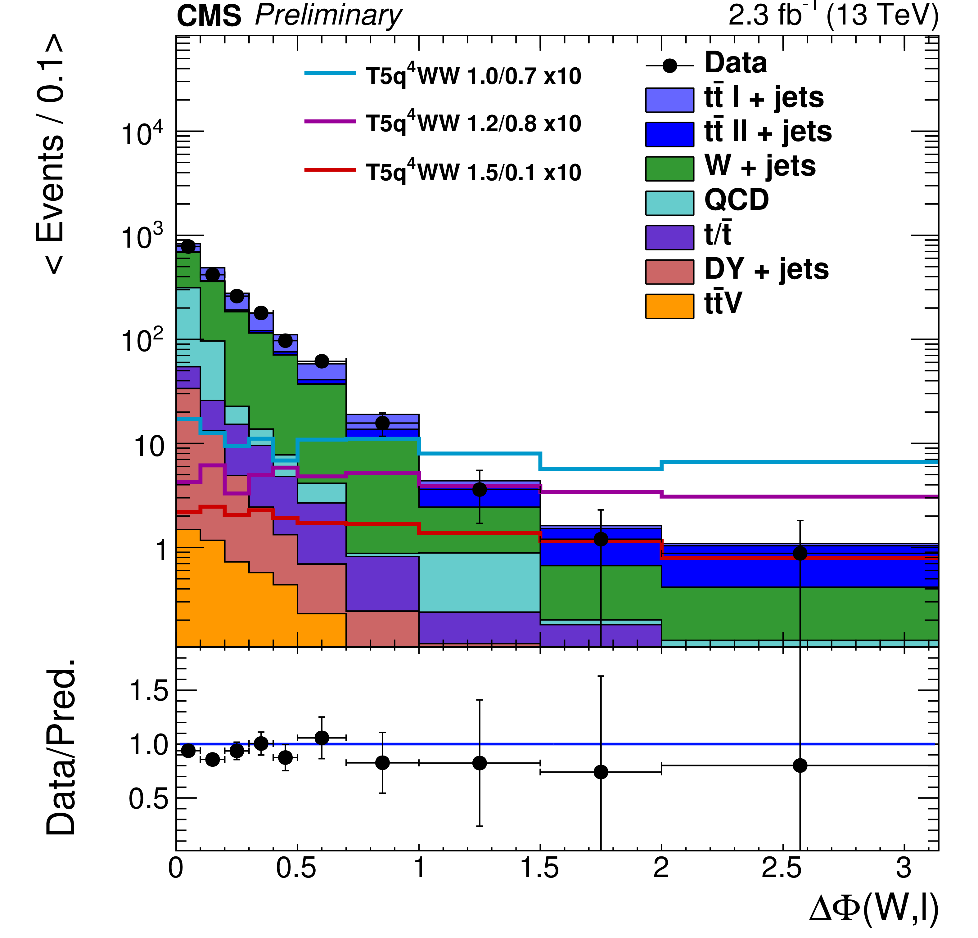
Comparison of the $ {\Delta \Phi } $ distribution for the multi-b (a) and zero-b analysis (b) after the preselection, requiring at least six jets for the multi-b analysis, of which at least one is b-tagged, and at least five jets for the zero-b analysis, with no b-tagged jet. A minimum $ {H_{\mathrm {T}}} $ of 500 GeV and a minimum $ {L_{\textrm T}} $ of 250 GeV is required in addition to exactly one lepton with $ {p_{\mathrm {T}}} >$ 25 GeV. The simulated background events are stacked on each other, and several signal points are overlayed without being stacked for illustration. For the multi-b analysis, the model T1t$^{4}$ 1.2/0.8 (T1t$^{4}$ 1.5/0.1) corresponds to a gluino mass of 1.2 TeV (1.5 TeV) and neutralino mass of 0.8 TeV (0.1 TeV), respectively. For the zero-b analysis, the model T5q$^{4}$WW 1.0/0.7 (T5q$^{4}$WW 1.2/0.8 and T5q$^{4}$WW 1.5/0.1) corresponds to a gluino mass of 1.0 TeV (1.2 TeV and 1.5 TeV) and neutralino mass of 0.7 TeV (0.8 TeV and 0.1 TeV), respectively. For the latter, the intermediate chargino mass is fixed at 0.85 TeV (1.0 TeV and 0.8 TeV). |
png pdf |
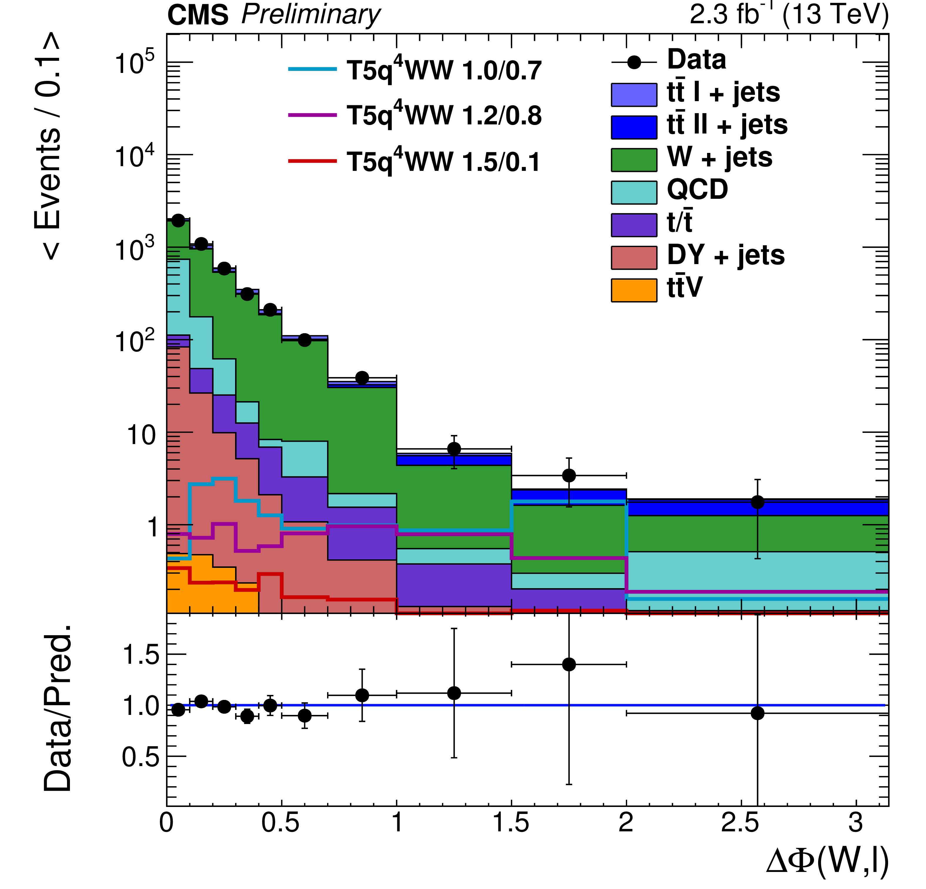
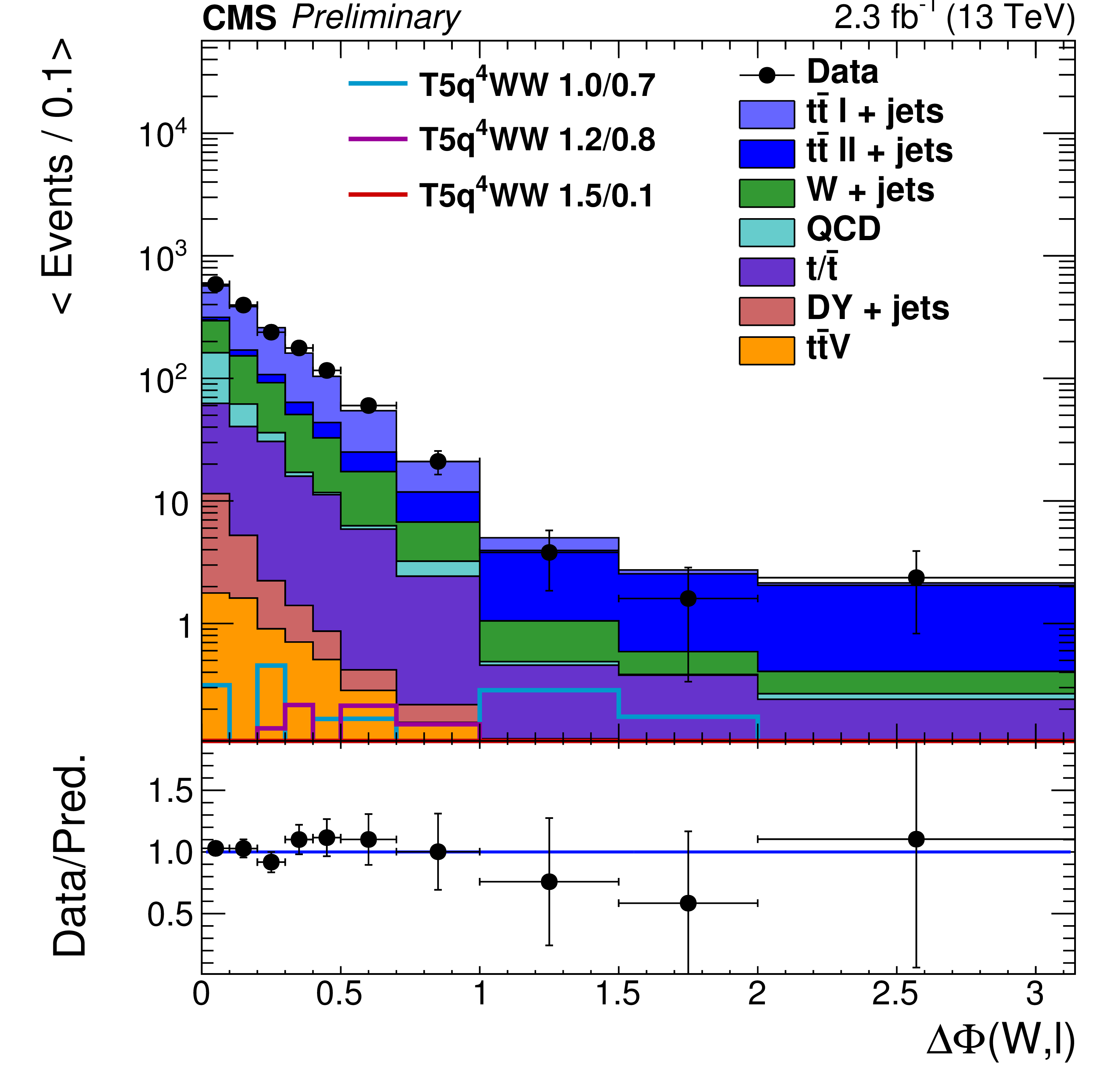
Figure 3-b:
Comparison of the $ {\Delta \Phi } $ distribution for the multi-b (a) and zero-b analysis (b) after the preselection, requiring at least six jets for the multi-b analysis, of which at least one is b-tagged, and at least five jets for the zero-b analysis, with no b-tagged jet. A minimum $ {H_{\mathrm {T}}} $ of 500 GeV and a minimum $ {L_{\textrm T}} $ of 250 GeV is required in addition to exactly one lepton with $ {p_{\mathrm {T}}} >$ 25 GeV. The simulated background events are stacked on each other, and several signal points are overlayed without being stacked for illustration. For the multi-b analysis, the model T1t$^{4}$ 1.2/0.8 (T1t$^{4}$ 1.5/0.1) corresponds to a gluino mass of 1.2 TeV (1.5 TeV) and neutralino mass of 0.8 TeV (0.1 TeV), respectively. For the zero-b analysis, the model T5q$^{4}$WW 1.0/0.7 (T5q$^{4}$WW 1.2/0.8 and T5q$^{4}$WW 1.5/0.1) corresponds to a gluino mass of 1.0 TeV (1.2 TeV and 1.5 TeV) and neutralino mass of 0.7 TeV (0.8 TeV and 0.1 TeV), respectively. For the latter, the intermediate chargino mass is fixed at 0.85 TeV (1.0 TeV and 0.8 TeV). |
png pdf |
Figure 4-a:
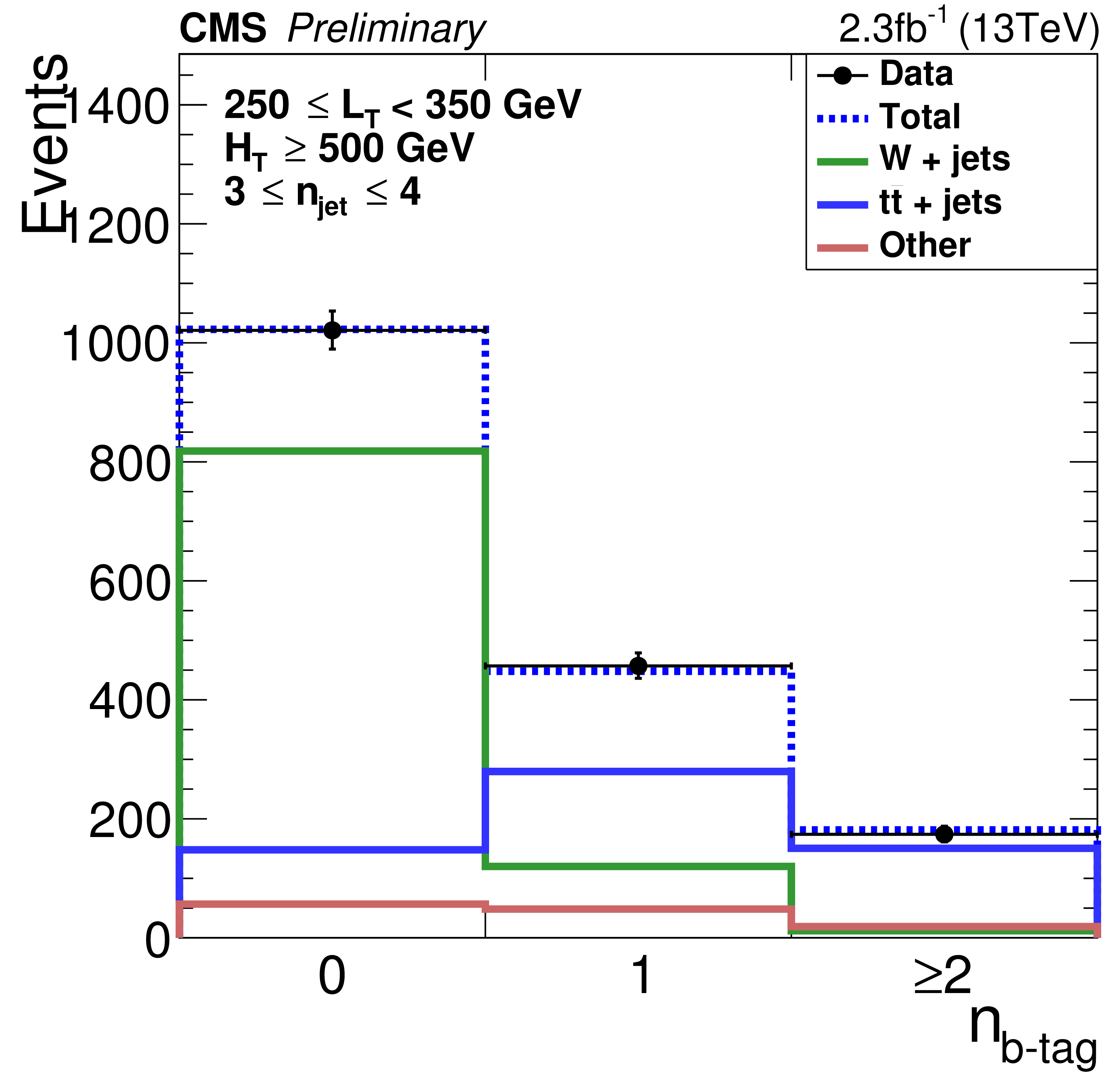
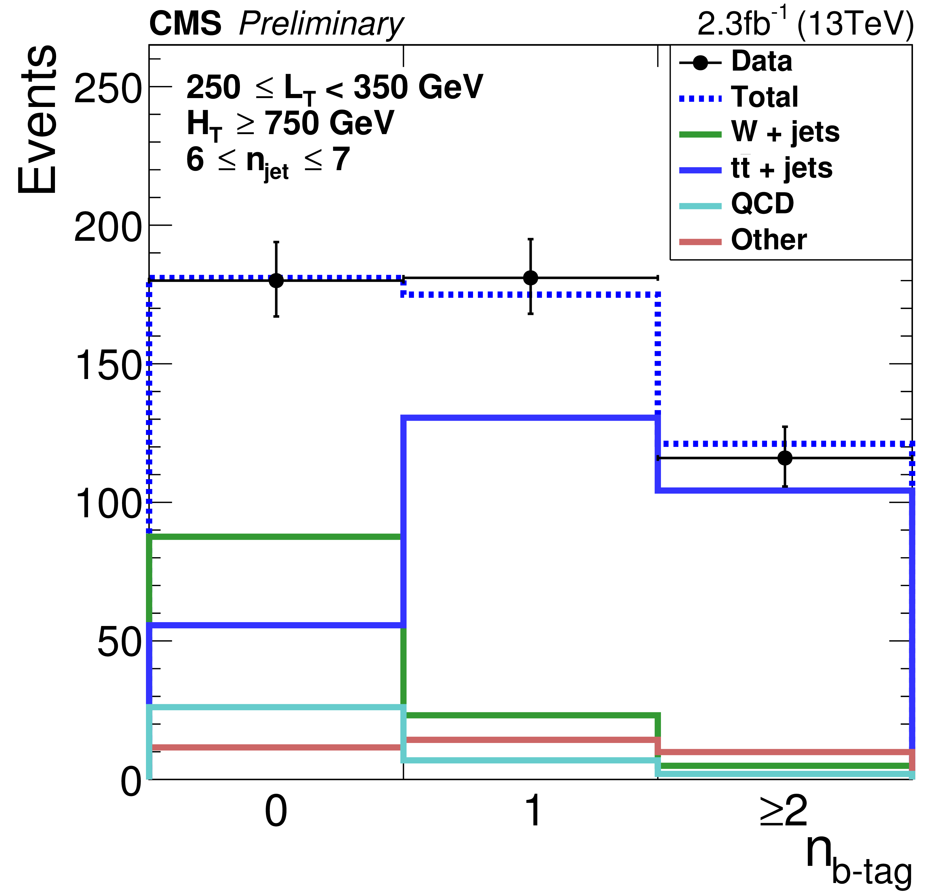
Fits to the $ {n_\textrm {b-tag}} $ multiplicity for control regions in (a) $3\leq {n_\textrm {jet}} \leq 4$ (250 $\leq {L_{\textrm T}} <$ 350 GeV, $ {H_{\mathrm {T}}} \geq$ 500GeV, $ {\Delta \Phi } <$ 1, muon channel) and (b) 6 $\leq {n_\textrm {jet}} \leq$ 7 (250 $\leq {L_{\textrm T}} <$ 350 GeV, ${H_{\mathrm {T}}} \geq $ 750 GeV, $ {\Delta \Phi } <$ 1) in data. The solid lines represent the templates scaled according to the fit result (blue for $ {\mathrm{ t \bar{t} } } $, green for W+jets, turquoise for QCD and red for the remaining backgrounds), the dashed line shows the sum after fit, and the markers represent data. |
png pdf |
Figure 4-b:
Fits to the $ {n_\textrm {b-tag}} $ multiplicity for control regions in (a) $3\leq {n_\textrm {jet}} \leq 4$ (250 $\leq {L_{\textrm T}} <$ 350 GeV, $ {H_{\mathrm {T}}} \geq$ 500GeV, $ {\Delta \Phi } <$ 1, muon channel) and (b) 6 $\leq {n_\textrm {jet}} \leq$ 7 (250 $\leq {L_{\textrm T}} <$ 350 GeV, ${H_{\mathrm {T}}} \geq $ 750 GeV, $ {\Delta \Phi } <$ 1) in data. The solid lines represent the templates scaled according to the fit result (blue for $ {\mathrm{ t \bar{t} } } $, green for W+jets, turquoise for QCD and red for the remaining backgrounds), the dashed line shows the sum after fit, and the markers represent data. |
png pdf |
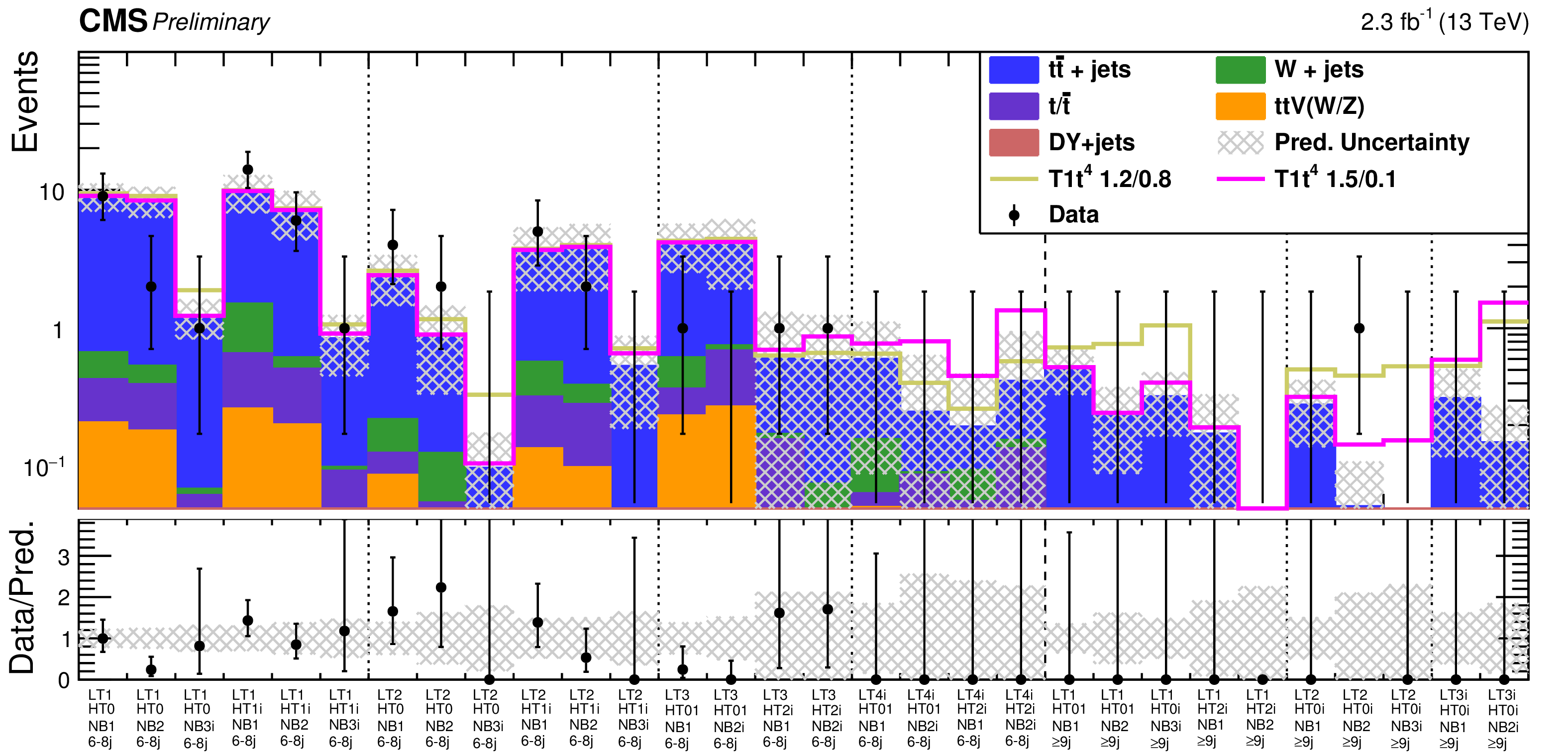
Figure 5:
Multi-b analysis: The data-driven prediction is represented by the filled histograms preserving the individual background contributions from MC; the observed number of events is shown in black. The colored lines show two signal benchmark points stacked on the prediction. |
png pdf |
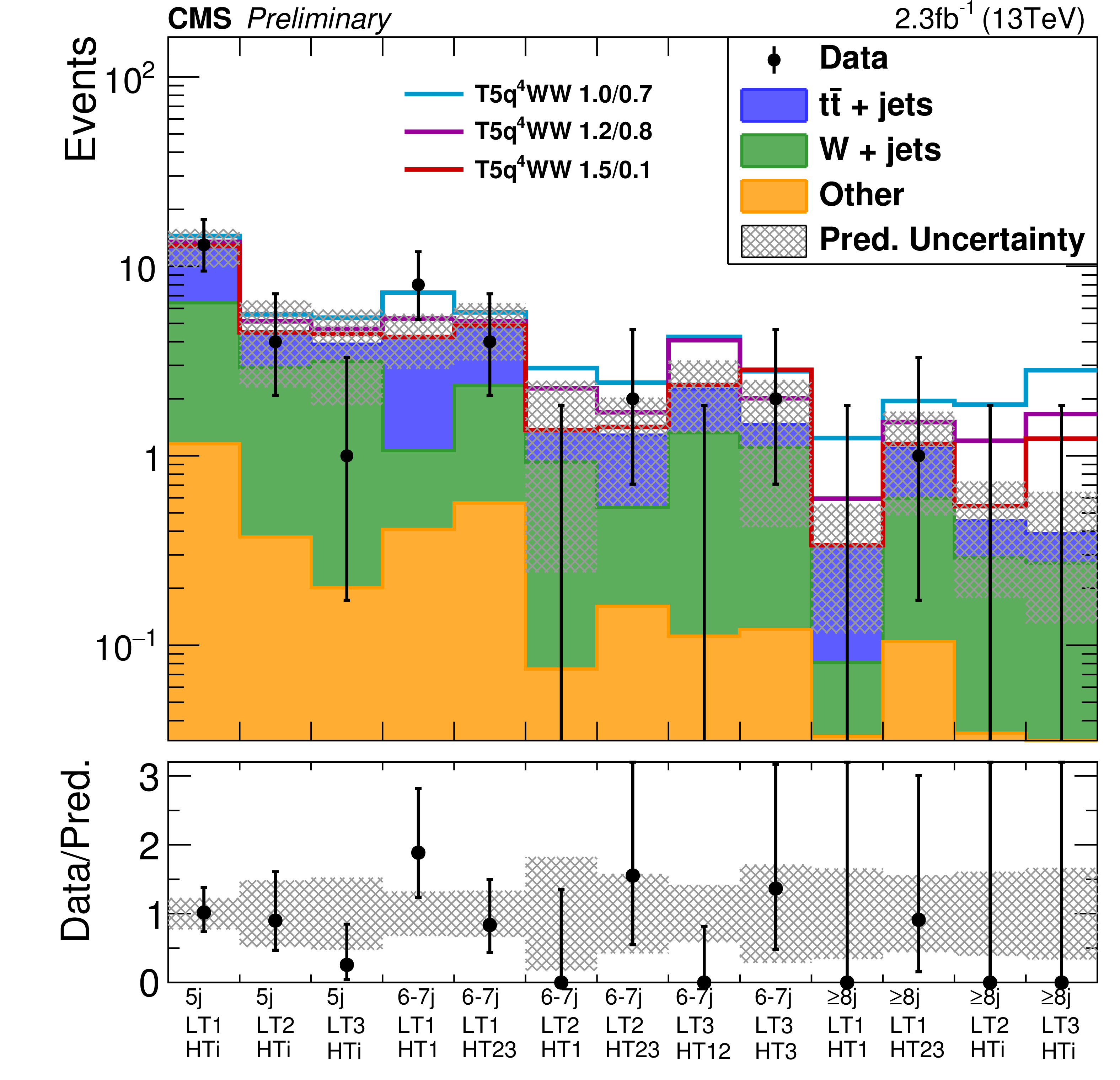
Figure 6:
Zero-b analysis: observed and predicted event counts in the 13 signal regions. The black points show the number of observed events. The filled, stacked histograms represent the predictions for $ {\mathrm{ t \bar{t} } } $, W+jets events, and the remaining backgrounds. The colored lines illustrate the expectations for three benchmark points of the T5q$^{4}$WW model. The lower panel shows the ratio between data and prediction. The error bars indicate the total statistical and systematic uncertainty on the ratio. |
png pdf |
Figure 7-a:
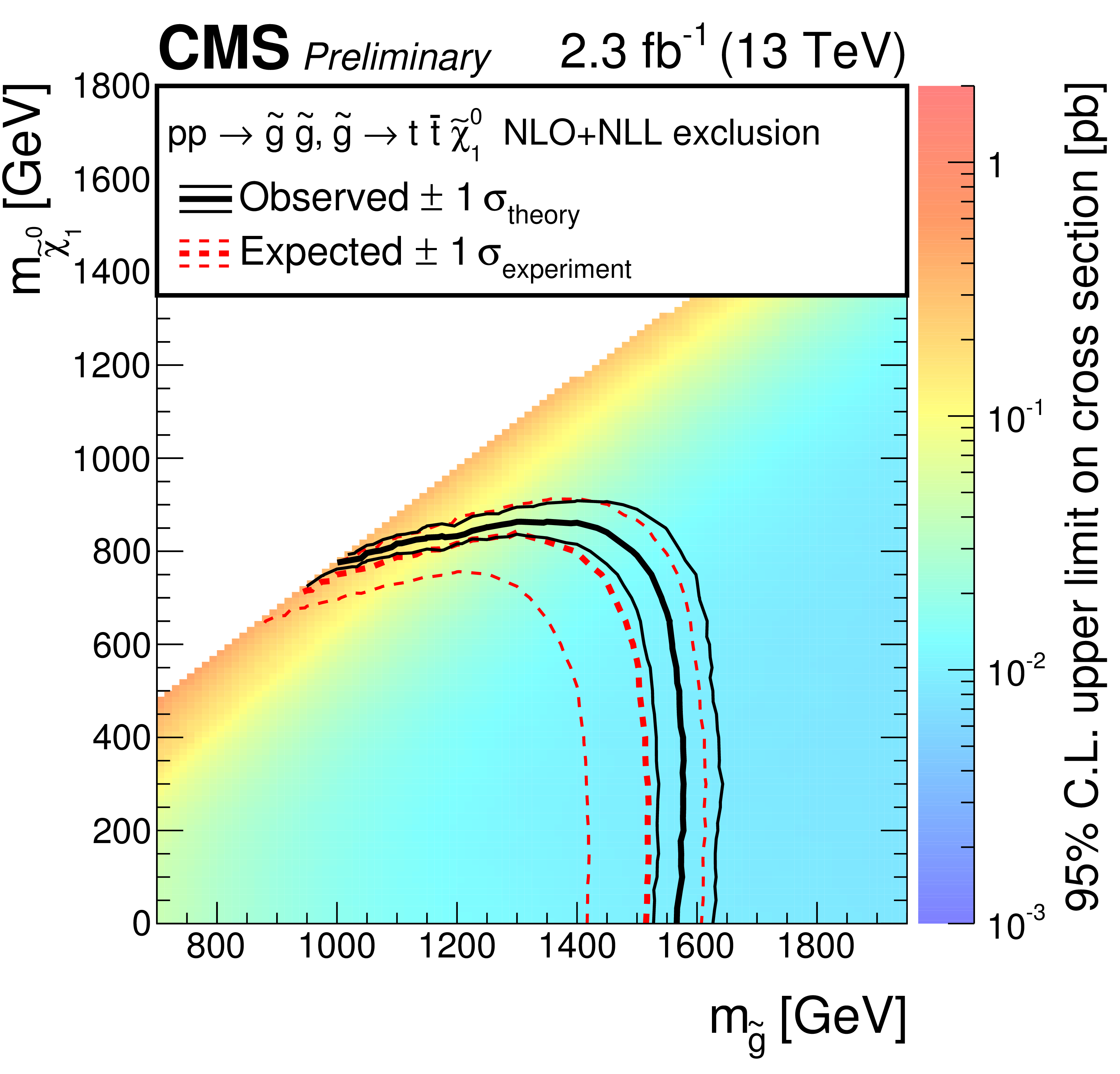
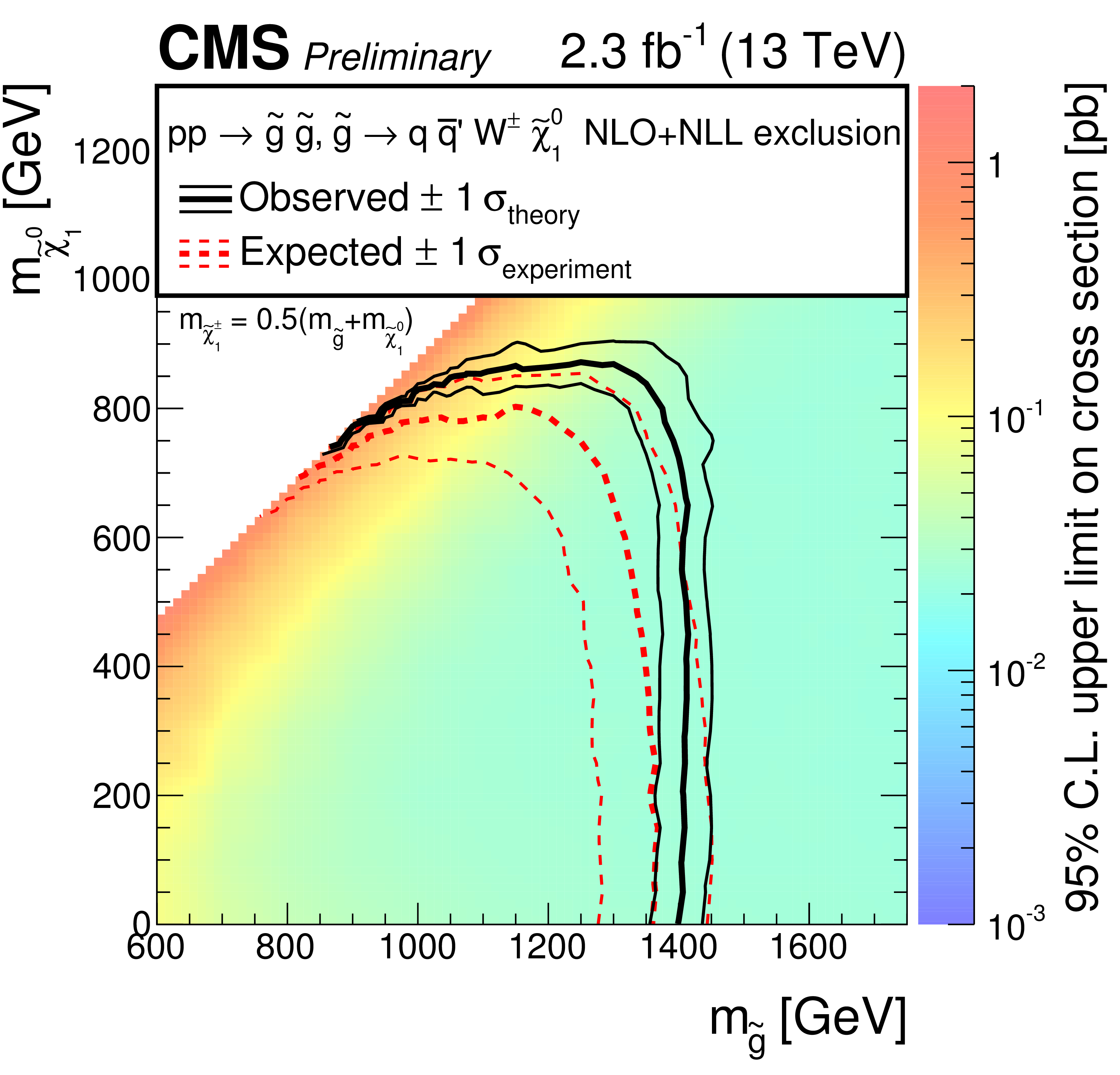
Cross section limits at 95% CL for the (a) T1t$^{4}$ and (b) T5q$^{4}$WW models as a function of the the gluino and LSP masses. In T5q$^{4}$WW, the pair-produced gluinos each decay to a quark-antiquark pair of the first or second generation ($ \mathrm{ q \bar{q} } $), and a chargino ($ {\tilde{\chi}^{\pm }_1} $) with its mass defined as $m_{ {\tilde{\chi}^{\pm }_1} }=0.5(m_{ \tilde{g} }+m_{ {\tilde{\chi}^0_1} })$. The black (red) lines correspond to the observed (expected) mass limits, with the solid lines representing the central values and the dashed lines the $\pm$1$\sigma $ uncertainty bands related to the theoretical (experimental) uncertainties. |
png pdf |
Figure 7-b:
Cross section limits at 95% CL for the (a) T1t$^{4}$ and (b) T5q$^{4}$WW models as a function of the the gluino and LSP masses. In T5q$^{4}$WW, the pair-produced gluinos each decay to a quark-antiquark pair of the first or second generation ($ \mathrm{ q \bar{q} } $), and a chargino ($ {\tilde{\chi}^{\pm }_1} $) with its mass defined as $m_{ {\tilde{\chi}^{\pm }_1} }=0.5(m_{ \tilde{g} }+m_{ {\tilde{\chi}^0_1} })$. The black (red) lines correspond to the observed (expected) mass limits, with the solid lines representing the central values and the dashed lines the $\pm$1$\sigma $ uncertainty bands related to the theoretical (experimental) uncertainties. |
| Tables | |
png pdf |
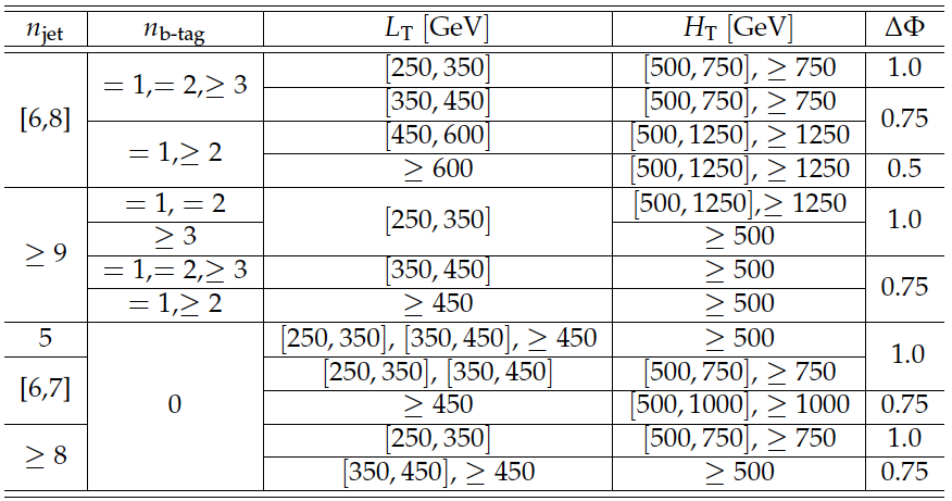
Table 1:
Signal regions and the corresponding $ {\Delta \Phi } $ requirement. |
png pdf |
Table 2:
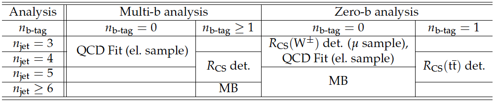
Overview of the definitions of sideband and mainband regions. |
png pdf |
Table 3:
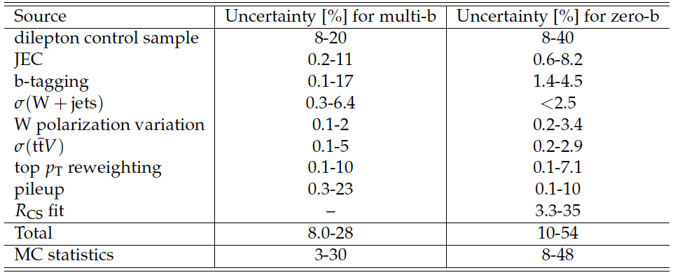
Summary of the systematic uncertainties for the total background prediction for the multi-b and for the zero-b analysis. |
png pdf |
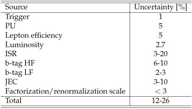
Table 4:
Summary of the systematic uncertainties and their average effect on the example signal points. The values are very similar for the multi-b and the zero-b analysis, and are mostly larger for compressed scenarios, where the mass difference between gluino and neutralino is small. |
png pdf |
Table 5:
Summary of the results in the multi-b search. |

png pdf |
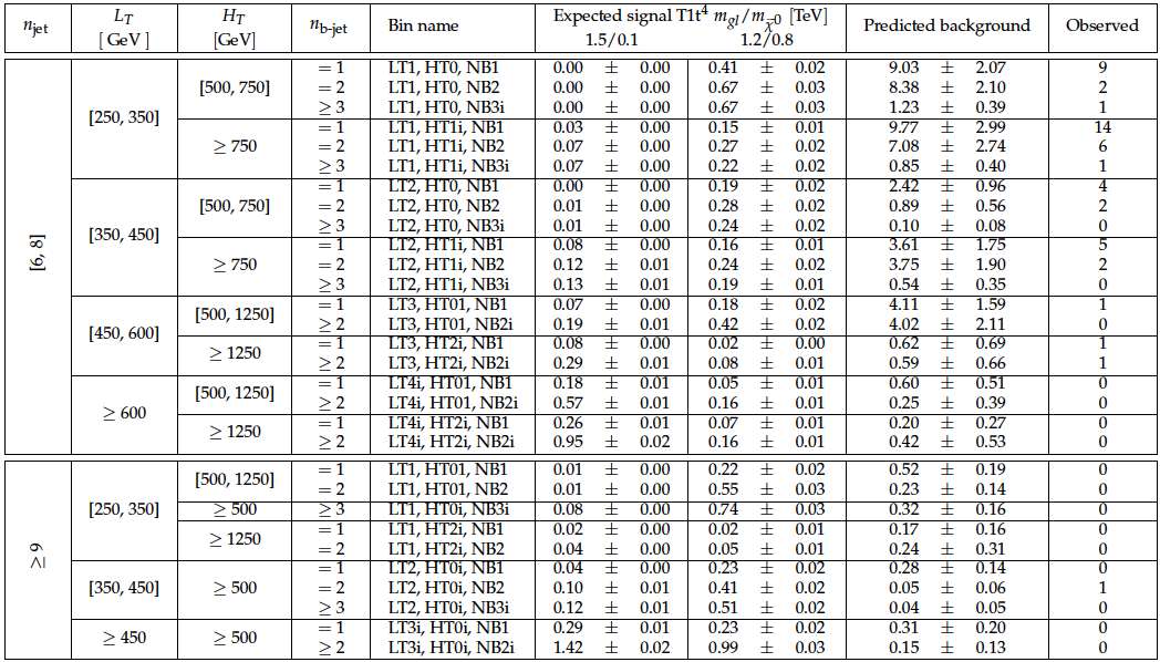
Table 6:
Summary of the results of the zero-b search with 2.3 fb$^{-1}$. |
png pdf |
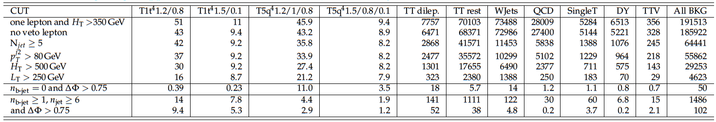
Table 7:
Yield table (2.3 fb$^{-1}$) for the baseline selection split for all backgrounds. The event yields in the last three lines are exclusive for the zero-b and the multi-b selection, respectively. The simulated events are corrected with scale factors to account for differences in the lepton identification and isolation efficiencies, as well as the b-tagging efficiency between simulation and data. The trigger efficiency is applied as well and a reweighting is applied to $ {\mathrm{ t \bar{t} } } $ events based on the $ {p_{\mathrm {T}}} $ of the $ {\mathrm{ t \bar{t} } } $ system. |
| Auxiliary Figures | |

png pdf |
Auxiliary Figure 1:
The number of b-tagged jets, after the preselection, requiring at least five jets. A minimum $ {H_{\mathrm {T}}} $ of 500 GeV and a minimum $ {L_{\textrm T}} $ of 250 GeV is required in addition to exactly one lepton with $ {p_{\mathrm {T}}} > 25$ GeV. The simulated background events are stacked on top of each other, and several signal points are overlaid for illustration without being stacked. The model T1t$^4$ 1.2/0.8 (T1t$^4$ 1.5/0.1) corresponds to a gluino mass of 1.2 TeV (1.5 TeV) and neutralino mass of 0.8 TeV (0.1 TeV), respectively. The model T5q$^4$WW 1.2/0.8 (T5q$^4$WW 1.5/0.1) corresponds to a gluino mass of 1.2 TeV (1.5 TeV) and neutralino mass of 0.8 TeV (0.1 TeV), respectively. For these models, the intermediate chargino mass is fixed at 1 TeV (0.8 TeV), respectively. |
png pdf |
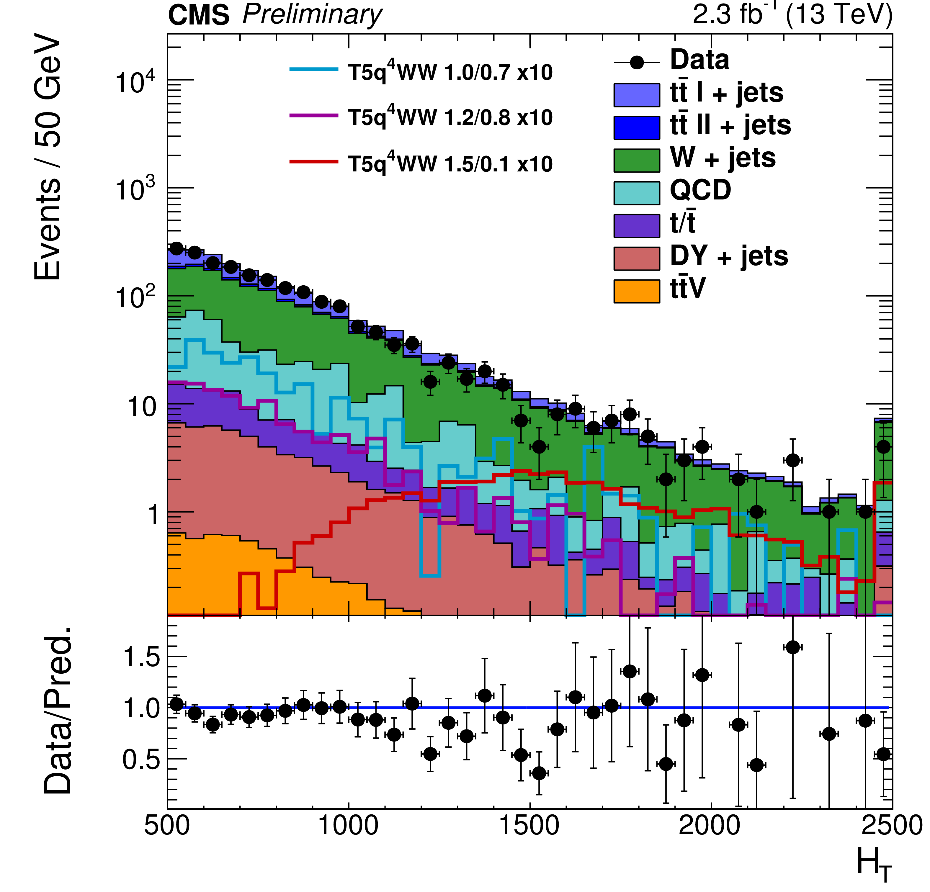
Auxiliary Figure 2:
The $ {H_{\mathrm {T}}} $ distribution for the zero-b analysis, after the preselection, requiring at least five jets, with no b-tagged jet. A minimum $ {H_{\mathrm {T}}} $ of 500 GeV and a minimum $ {L_{\textrm T}} $ of 250 GeV is required in addition to exactly one lepton with $ {p_{\mathrm {T}}} > 25$ GeV. The simulated background events are stacked on top of each other, and several signal points are overlaid for illustration without being stacked. The model T5q$^4$WW 1.0/0.7 (T5q$^4$WW 1.2/0.8 and T5q$^4$WW 1.5/0.1) corresponds to a gluino mass of 1.0 TeV (1.2 TeV and 1.5 TeV) and neutralino mass of 0.7 TeV (0.8 TeV and 0.1 TeV), respectively. For the latter, the intermediate chargino mass is fixed at 0.85 TeV (1.0 TeV and 0.8 TeV). |
png pdf |
Auxiliary Figure 3:
The $ {L_{\textrm T}} $ distribution for the multi-b analysis, after the preselection, requiring at least six jets, of which at least one is b-tagged. A minimum $ {H_{\mathrm {T}}} $ of 500 GeV and a minimum $ {L_{\textrm T}} $ of 250 GeV is required in addition to exactly one lepton with $ {p_{\mathrm {T}}} > 25$ GeV. The simulated background events are stacked on top of each other, and several signal points are overlaid for illustration without being stacked. The model T1t$^4$ 1.2/0.8 (T1t$^4$ 1.5/0.1) corresponds to a gluino mass of 1.2 TeV (1.5 TeV) and neutralino mass of 0.8 TeV (0.1 TeV), respectively. |
png pdf |
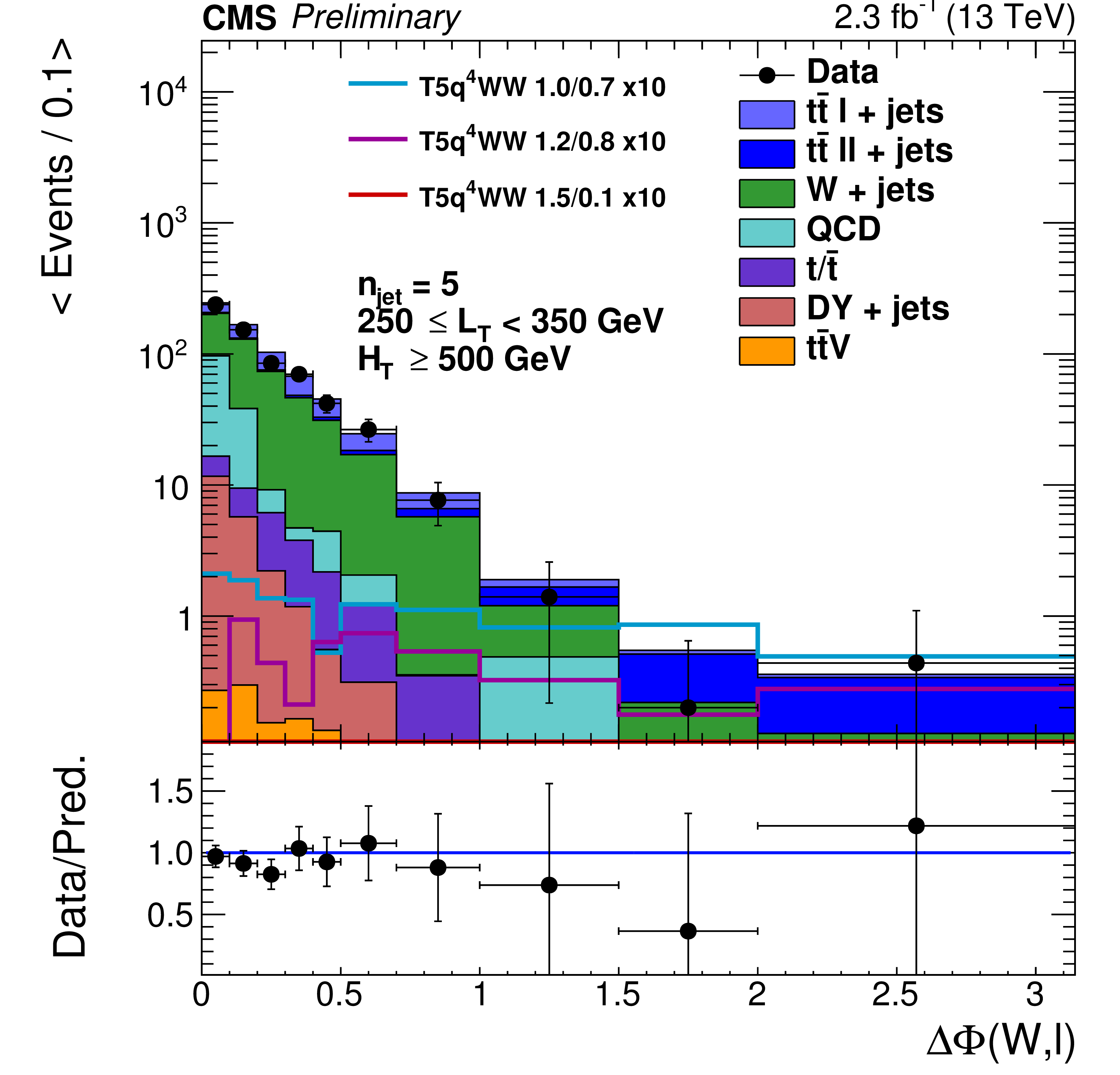
Auxiliary Figure 4:
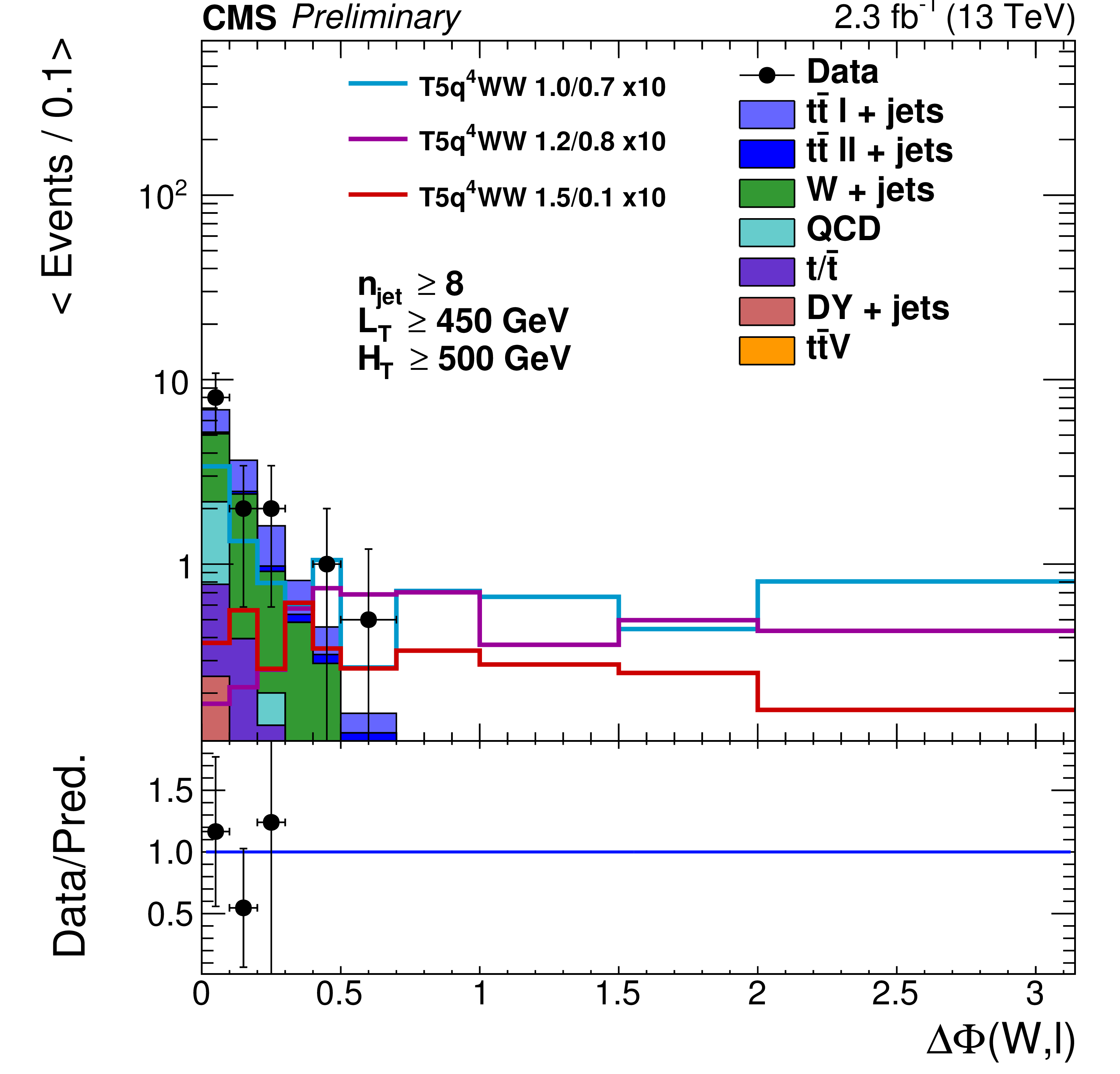
The $ {\Delta \Phi } $ distribution for the zero-b analysis, after the preselection, requiring five jets, with no b-tagged jet. A minimum $ {H_{\mathrm {T}}} $ of 500 GeV and $250 GeV < {L_{\textrm T}} <350$ GeV is required in addition to exactly one lepton with $ {p_{\mathrm {T}}} > 25$ GeV. The simulated background events are stacked on top of each other, and several signal points are overlaid for illustration without being stacked. The model T5q$^4$WW 1.0/0.7 (T5q$^4$WW 1.2/0.8 and T5q$^4$WW 1.5/0.1) corresponds to a gluino mass of 1.0 TeV (1.2 TeV and 1.5 TeV) and neutralino mass of 0.7 TeV (0.8 TeV and 0.1 TeV), respectively. For the latter, the intermediate chargino mass is fixed at 0.85 TeV (1.0 TeV and 0.8 TeV). |
png pdf |
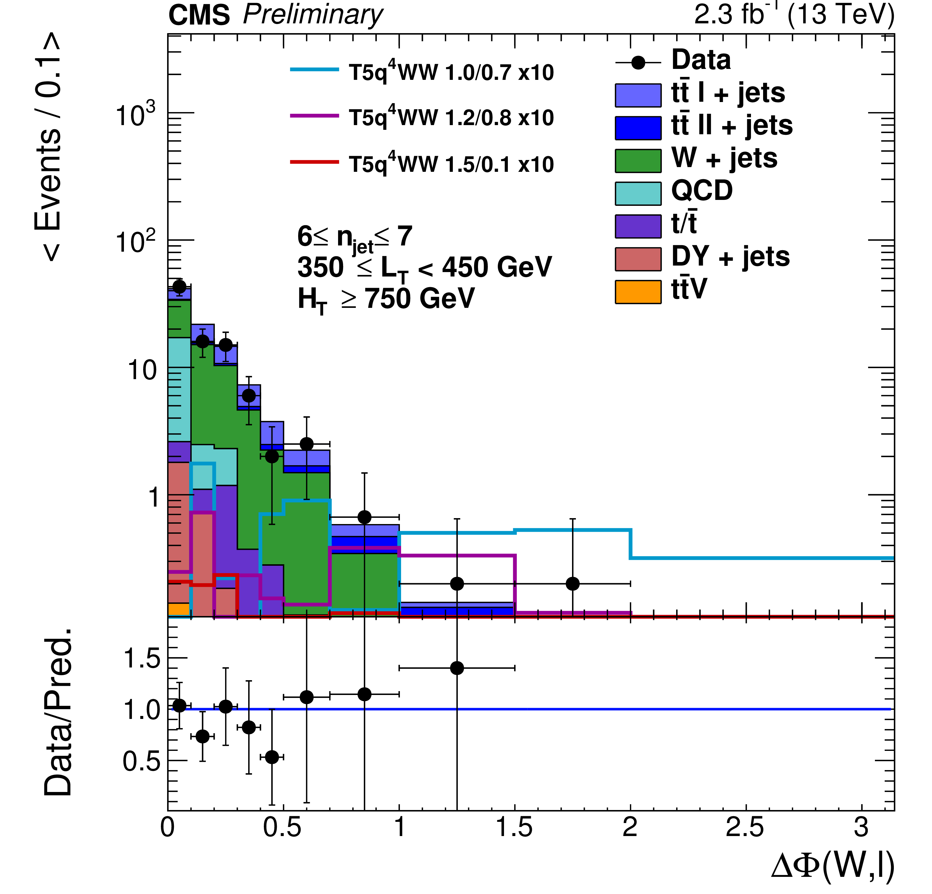
Auxiliary Figure 5:
The $ {\Delta \Phi } $ distribution for the zero-b analysis, after the preselection, requiring six or seven jets, with no b-tagged jet. A minimum $ {H_{\mathrm {T}}} $ of 750 GeV and 350 GeV $< {L_{\textrm T}} <$ 450 GeV is required in addition to exactly one lepton with $ {p_{\mathrm {T}}} >$ 25 GeV. The simulated background events are stacked on top of each other, and several signal points are overlaid for illustration without being stacked. The model T5q$^4$WW 1.0/0.7 (T5q$^4$WW 1.2/0.8 and T5q$^4$WW 1.5/0.1) corresponds to a gluino mass of 1.0 TeV (1.2 TeV and 1.5 TeV) and neutralino mass of 0.7 TeV (0.8 TeV and 0.1 TeV), respectively. For the latter, the intermediate chargino mass is fixed at 0.85 TeV (1.0 TeV and 0.8 TeV). |
png pdf |
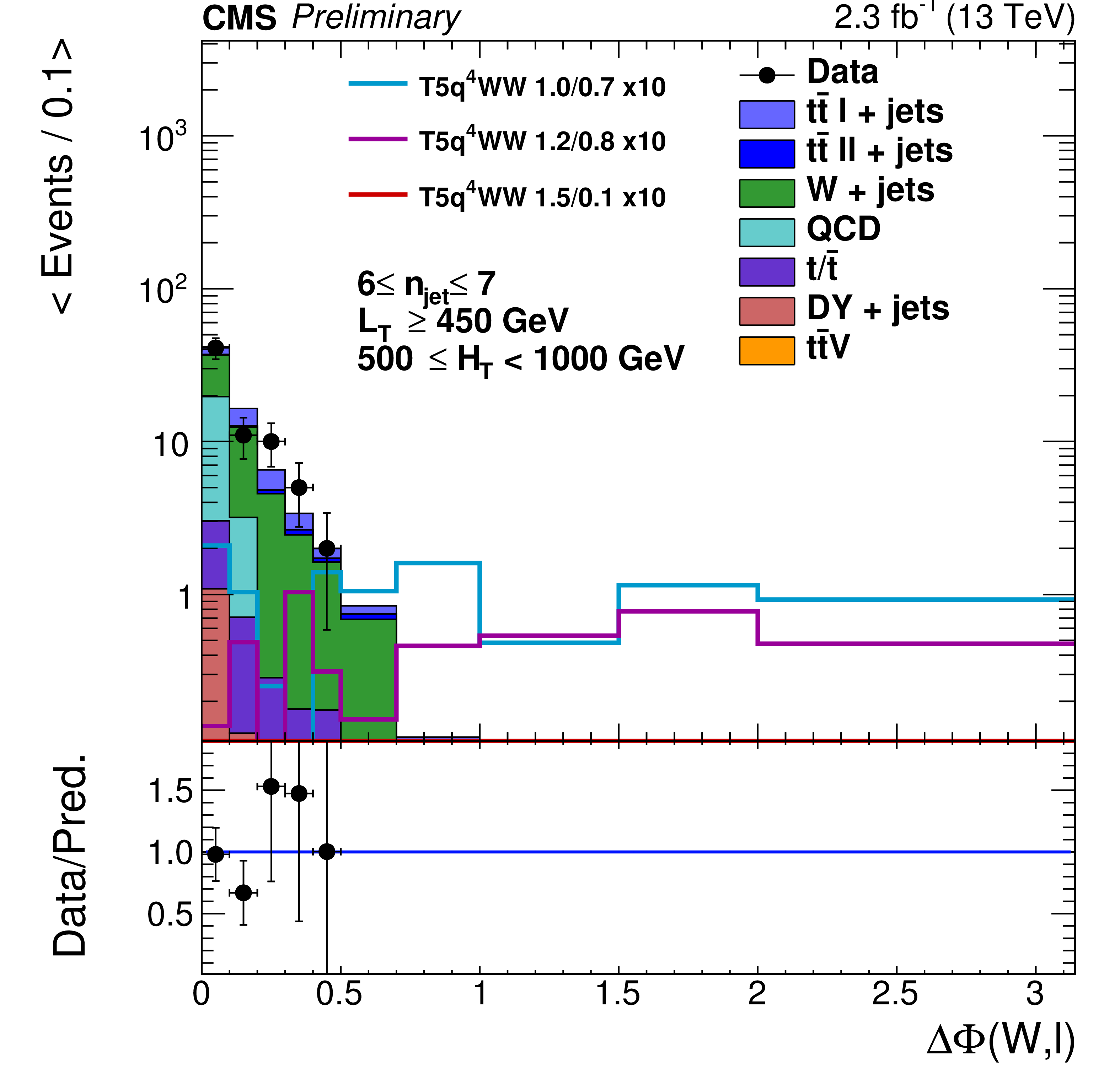
Auxiliary Figure 6:
The $ {\Delta \Phi } $ distribution for the zero-b analysis, after the preselection, requiring six or seven jets, with no b-tagged jet. A cut on 500 GeV $< {H_{\mathrm {T}}} <$ 1000 GeV and $ {L_{\textrm T}} >$ 450 GeV is required in addition to exactly one lepton with $ {p_{\mathrm {T}}} >$ 25 GeV. The simulated background events are stacked on top of each other, and several signal points are overlaid for illustration without being stacked. The model T5q$^4$WW 1.0/0.7 (T5q$^4$WW 1.2/0.8 and T5q$^4$WW 1.5/0.1) corresponds to a gluino mass of 1.0 TeV (1.2 TeV and 1.5 TeV) and neutralino mass of 0.7 TeV (0.8 TeV and 0.1 TeV), respectively. For the latter, the intermediate chargino mass is fixed at 0.85 TeV (1.0 TeV and 0.8 TeV). |
png pdf |
Auxiliary Figure 7:
The $ {\Delta \Phi } $ distribution for the zero-b analysis, after the preselection, requiring at least eight jets, with no b-tagged jet. A minimum $ {H_{\mathrm {T}}} $ of 500 GeV and $ {L_{\textrm T}} >$ 450 GeV is required in addition to exactly one lepton with $ {p_{\mathrm {T}}} >$ 25 GeV. The simulated background events are stacked on top of each other, and several signal points are overlaid for illustration without being stacked. The model T5q$^4$WW 1.0/0.7 (T5q$^4$WW 1.2/0.8 and T5q$^4$WW 1.5/0.1) corresponds to a gluino mass of 1.0 TeV (1.2 TeV and 1.5 TeV) and neutralino mass of 0.7 TeV (0.8 TeV and 0.1 TeV), respectively. For the latter, the intermediate chargino mass is fixed at 0.85 TeV (1.0 TeV and 0.8 TeV). |
png pdf |
Auxiliary Figure 8:
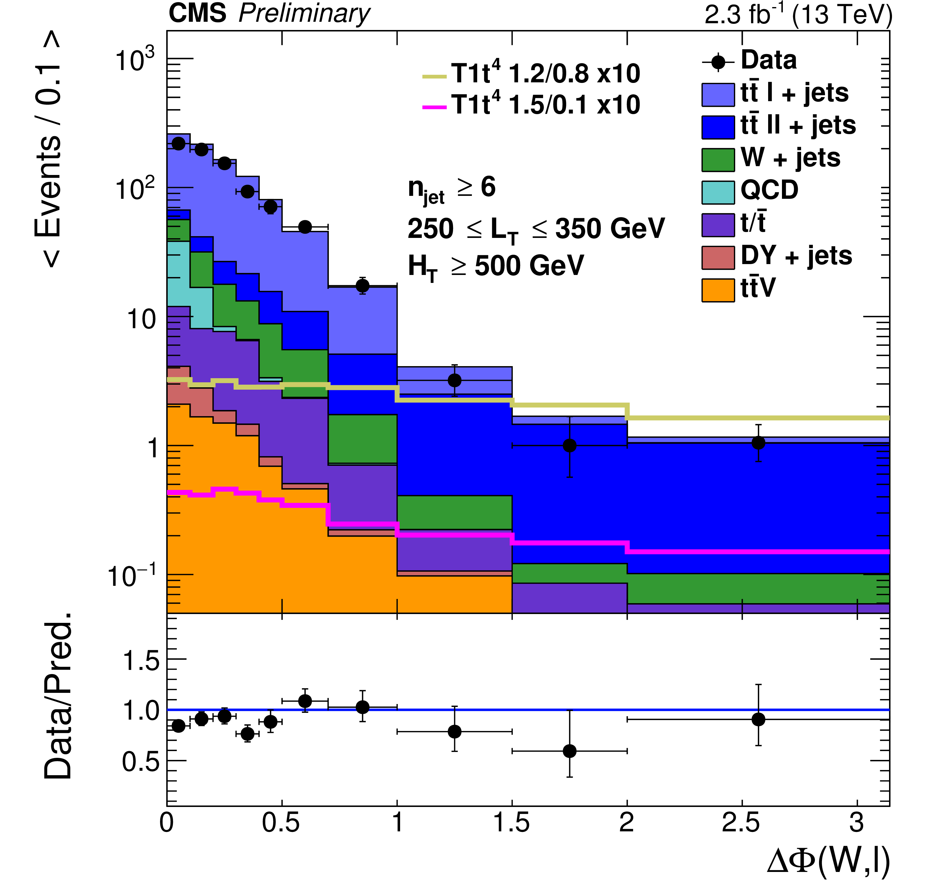
The $ {\Delta \Phi } $ distribution for the multi-b analysis, after the preselection, requiring at least six jets, of which at least one is b-tagged. A minimum $ {H_{\mathrm {T}}} $ of 500 GeV and 250 GeV $ < {L_{\textrm T}} <$ 350 GeV is required in addition to exactly one lepton with $ {p_{\mathrm {T}}} >$ 25 GeV. The simulated background events are stacked on top of each other, and several signal points are overlaid for illustration without being stacked. The model T1t$^4$ 1.2/0.8 (T1t$^4$ 1.5/0.1) corresponds to a gluino mass of 1.2 TeV (1.5 TeV) and neutralino mass of 0.8 TeV (0.1 TeV), respectively. |
png pdf |
Auxiliary Figure 9:
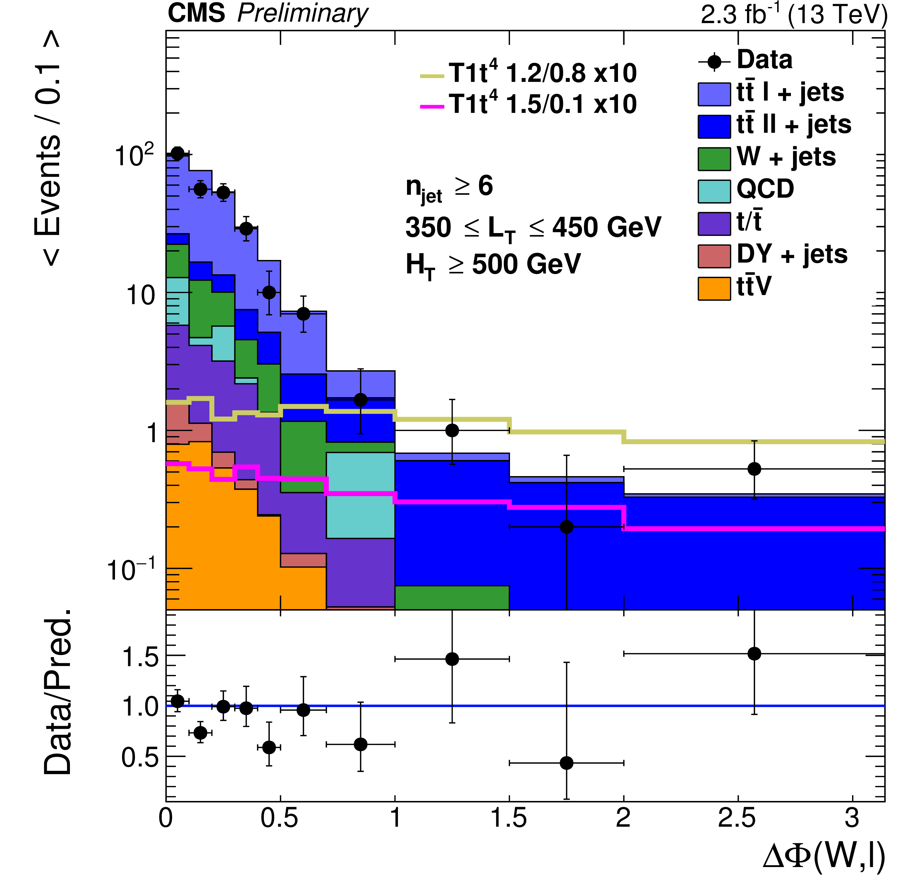
The $ {\Delta \Phi } $ distribution for the multi-b analysis, after the preselection, requiring at least six jets, of which at least one is b-tagged. A minimum $ {H_{\mathrm {T}}} $ of 500 GeV and 350 GeV $ < {L_{\textrm T}} <$ 450 GeV is required in addition to exactly one lepton with $ {p_{\mathrm {T}}} >$ 25 GeV. The simulated background events are stacked on top of each other, and several signal points are overlaid for illustration without being stacked. The model T1t$^4$ 1.2/0.8 (T1t$^4$ 1.5/0.1) corresponds to a gluino mass of 1.2 TeV (1.5 TeV) and neutralino mass of 0.8 TeV (0.1 TeV), respectively. |
png pdf |
Auxiliary Figure 10:
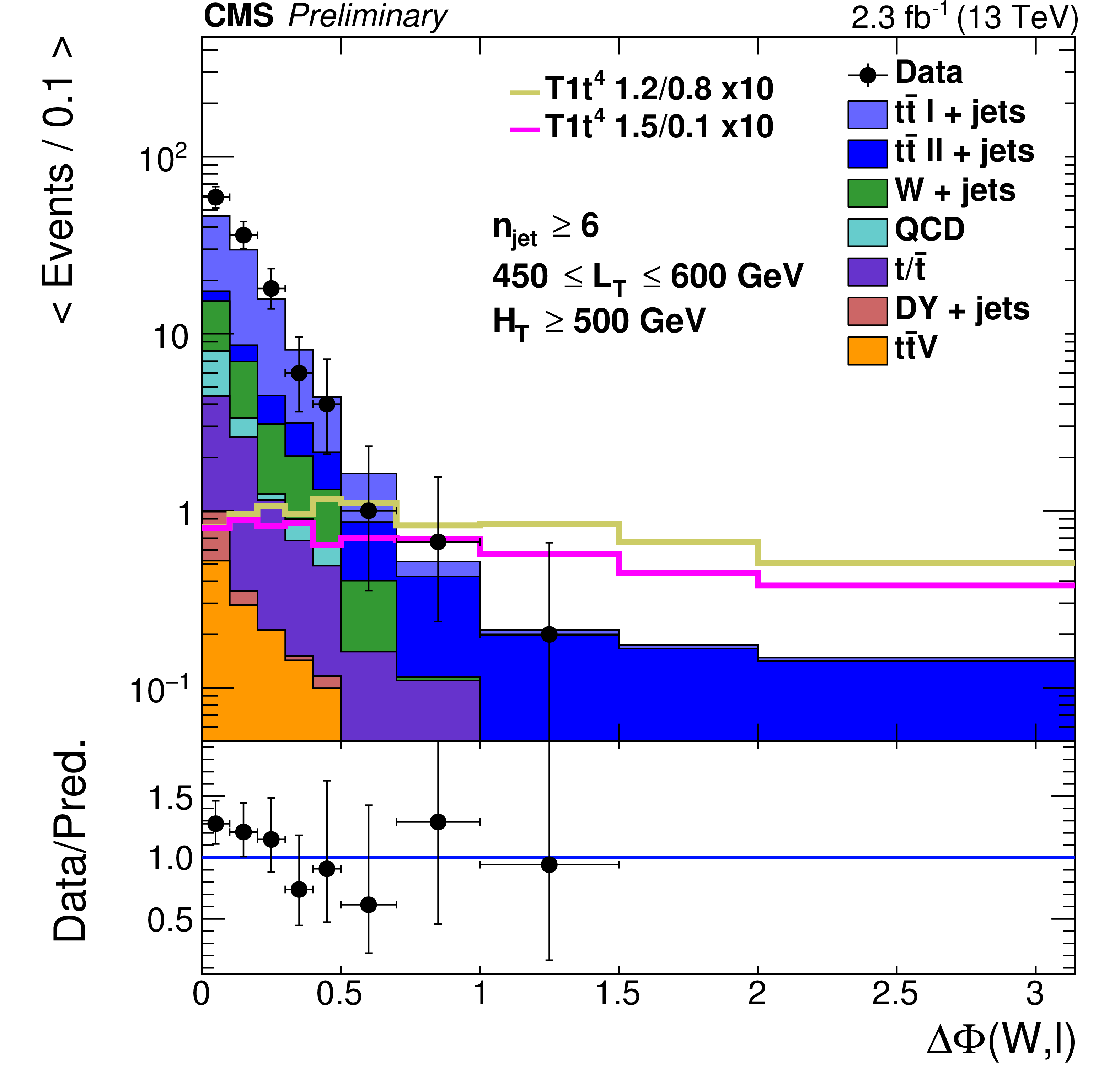
The $ {\Delta \Phi } $ distribution for the multi-b analysis, after the preselection, requiring at least six jets, of which at least one is b-tagged. A minimum $ {H_{\mathrm {T}}} $ of 500 GeV and 450 GeV $ < {L_{\textrm T}} <600$ GeV is required in addition to exactly one lepton with $ {p_{\mathrm {T}}} > 25$ GeV. The simulated background events are stacked on top of each other, and several signal points are overlaid for illustration without being stacked. The model T1t$^4$ 1.2/0.8 (T1t$^4$ 1.5/0.1) corresponds to a gluino mass of 1.2 TeV (1.5 TeV) and neutralino mass of 0.8 TeV (0.1 TeV), respectively. |

png pdf |
Auxiliary Figure 11:
The $ {\Delta \Phi } $ distribution for the multi-b analysis, after the preselection, requiring at least six jets, of which at least one is b-tagged. A minimum $ {H_{\mathrm {T}}} $ of 500 GeV and $ {L_{\textrm T}} >$ 600 GeV is required in addition to exactly one lepton with $ {p_{\mathrm {T}}} >$ 25 GeV. The simulated background events are stacked on top of each other, and several signal points are overlaid for illustration without being stacked. The model T1t$^4$ 1.2/0.8 (T1t$^4$ 1.5/0.1) corresponds to a gluino mass of 1.2 TeV (1.5 TeV) and neutralino mass of 0.8 TeV (0.1 TeV), respectively. |
png pdf |
Auxiliary Figure 12:
The $ {\Delta \Phi } $ distribution for the zero-b analysis, in the W+jets sideband. A minimum $ {H_{\mathrm {T}}} $ of 500 GeV and $ {L_{\textrm T}} >$ 250 GeV is required in addition to exactly one lepton with $ {p_{\mathrm {T}}} >$ 25 GeV. The simulated background events are stacked on top of each other, and several signal points are overlaid for illustration without being stacked. The model T5q$^4$WW 1.0/0.7 (T5q$^4$WW 1.2/0.8 and T5q$^4$WW 1.5/0.1) corresponds to a gluino mass of 1.0 TeV (1.2 TeV and 1.5 TeV) and neutralino mass of 0.7 TeV (0.8 TeV and 0.1 TeV), respectively. For the latter, the intermediate chargino mass is fixed at 0.85 TeV (1.0 TeV and 0.8 TeV). |
png pdf |
Auxiliary Figure 13:
The $ {\Delta \Phi } $ distribution for the zero-b analysis, in the $ {\mathrm{ t \bar{t} } } $ sideband. A minimum $ {H_{\mathrm {T}}} $ of 500 GeV and $ {L_{\textrm T}} >$ 250 GeV is required in addition to exactly one lepton with $ {p_{\mathrm {T}}} >$ 25 GeV. The simulated background events are stacked on top of each other, and several signal points are overlaid for illustration without being stacked. The model T5q$^4$WW 1.0/0.7 (T5q$^4$WW 1.2/0.8 and T5q$^4$WW 1.5/0.1) corresponds to a gluino mass of 1.0 TeV (1.2 TeV and 1.5 TeV) and neutralino mass of 0.7 TeV (0.8 TeV and 0.1 TeV), respectively. For the latter, the intermediate chargino mass is fixed at 0.85 TeV (1.0 TeV and 0.8 TeV). |
png pdf |
Auxiliary Figure 14:
The $ {\Delta \Phi } $ distribution for the sideband of the multi-b analysis, after the preselection, requiring four of five jets, of which at least one is b-tagged. A minimum $ {H_{\mathrm {T}}} $ of 500 GeV and $ {L_{\textrm T}} >600$ GeV is required in addition to exactly one lepton with $ {p_{\mathrm {T}}} >$ 25 GeV. The simulated background events are stacked on top of each other, and several signal points are overlaid for illustration without being stacked. The model T1t$^4$ 1.2/0.8 (T1t$^4$ 1.5/0.1) corresponds to a gluino mass of 1.2 TeV (1.5 TeV) and neutralino mass of 0.8 TeV (0.1 TeV), respectively. |

png pdf |
Auxiliary Figure 15:
The $ {R_{\textrm {CS}}} $ values from simulation (excluding the QCD sample) and $\kappa _{\rm EWK}$ for all signal regions of the multi-b analysis. |
png pdf |
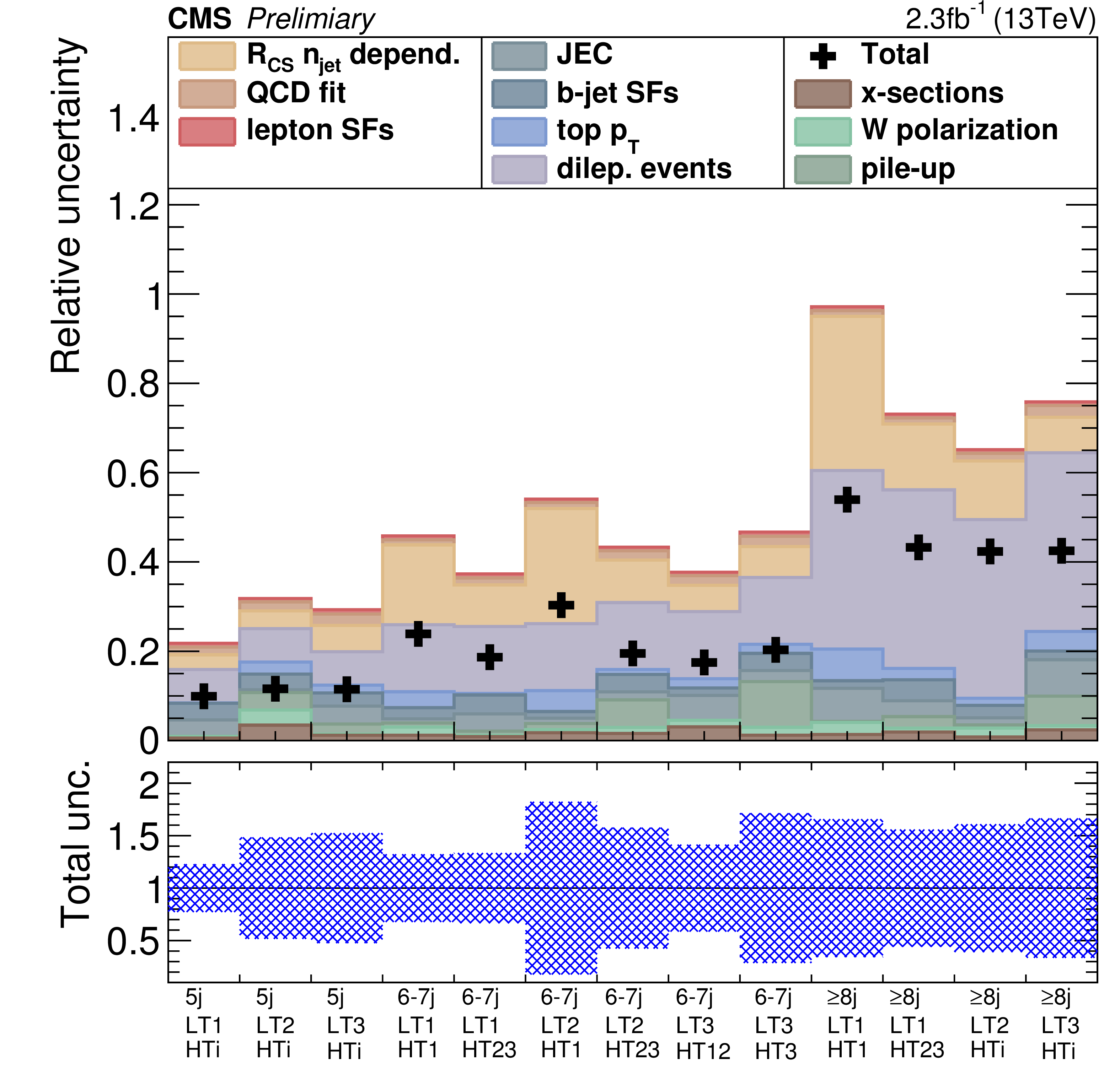
Auxiliary Figure 16:
The systematic uncertainties for all signal regions of the zero-b analysis. The top part of the plot shows the relative uncertainty on the background prediction for the different sources of uncertainties. The various uncertainties are stacked linearly on top of each other, while the black crosses represent the square root of the sum of squares. The bottom part of the plot shows the total relative uncertainty, including statistical and systematic terms, as a blue dotted area around unity. |

png pdf |
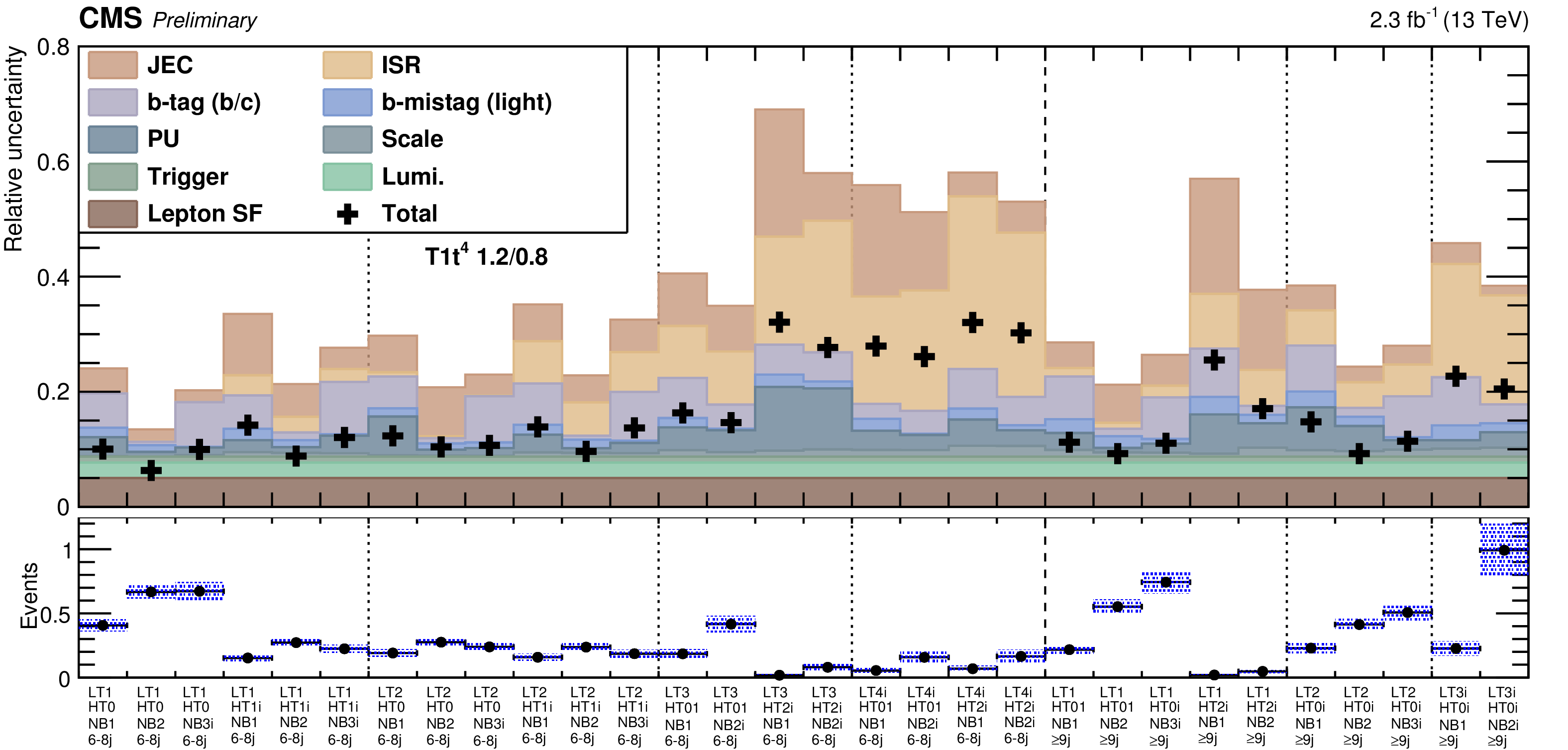
Auxiliary Figure 17:
The systematic uncertainties for all signal regions of the zero-b analysis. The top part of the plot shows the relative uncertainty for an example signal point (T5q$^4$WW 1.2/0.8) for the different sources of uncertainties. The various uncertainties are stacked linearly on top of each other, while the black crosses represent the square root of the sum of squares. The bottom part of the plot shows the expected yields for each signal region with the statistical uncertainty represented by the black line and the sum of statistical and systematic uncertainty by the blue dotted area. |
png pdf |
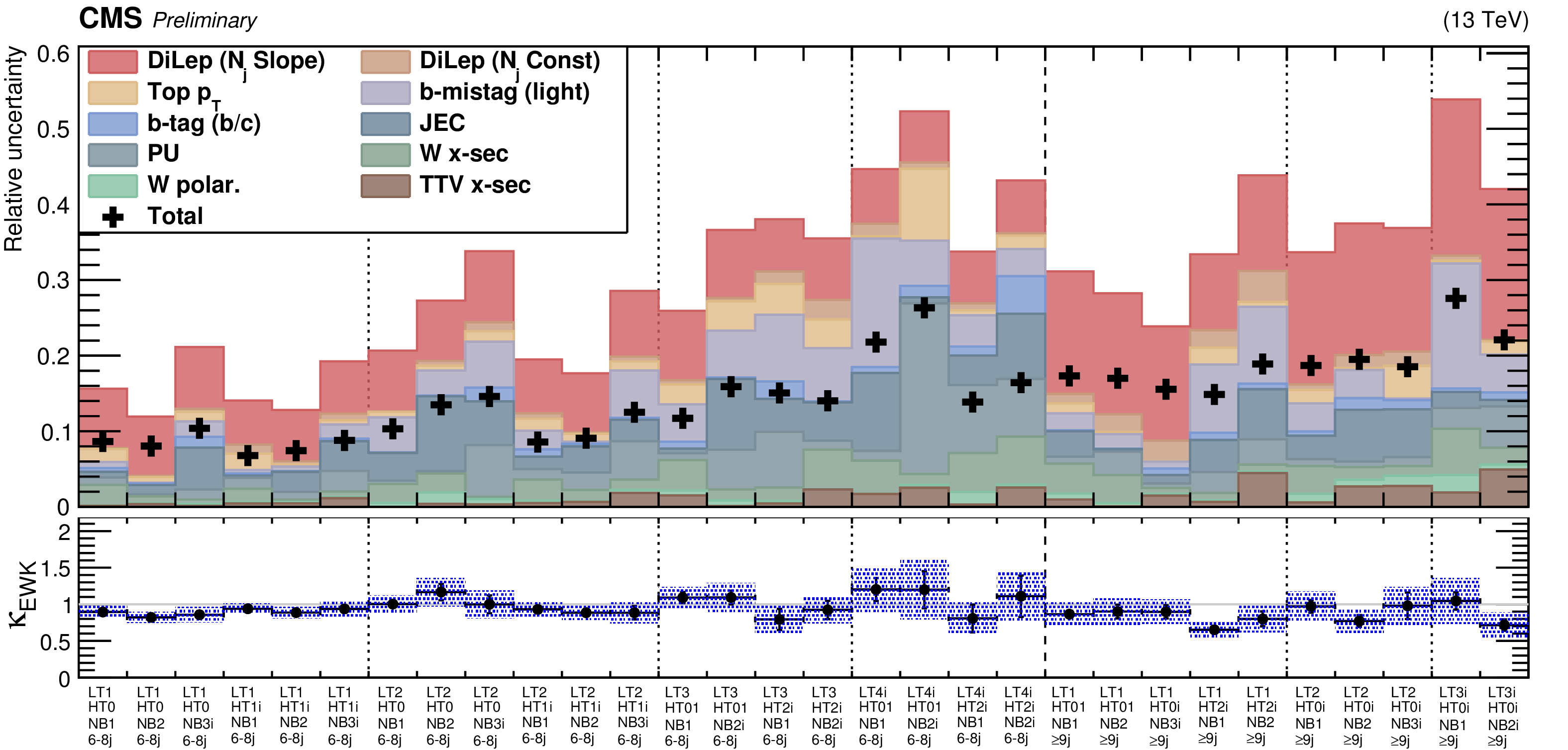
Auxiliary Figure 18:
The systematic uncertainties for all signal regions of the multi-b analysis.The top part of the plot shows the relative uncertainty on the background prediction for the different sources of uncertainties. The various uncertainties are stacked linearly on top of each other, while the black crosses represent the square root of the sum of squares. The bottom part of the plot shows the nominal $\kappa $ values with the statistical uncertainty represented by the black line and the sum of statistical and systematic uncertainty shown by the blue dotted area. |
png pdf |
Auxiliary Figure 19:
The systematic uncertainties for all signal regions of the multi-b analysis.The top part of the plot shows the relative uncertainty for an example signal point (T5t$^4$WW 1.2/0.8) for the different sources of uncertainties. The various uncertainties are stacked linearly on top of each other, while the black crosses represent the square root of the sum of squares. The bottom part of the plot shows the nominal $\kappa $ values with the statistical uncertainty represented by the black line and the sum of statistical and systematic uncertainty shown by the blue dotted area. |
png pdf |
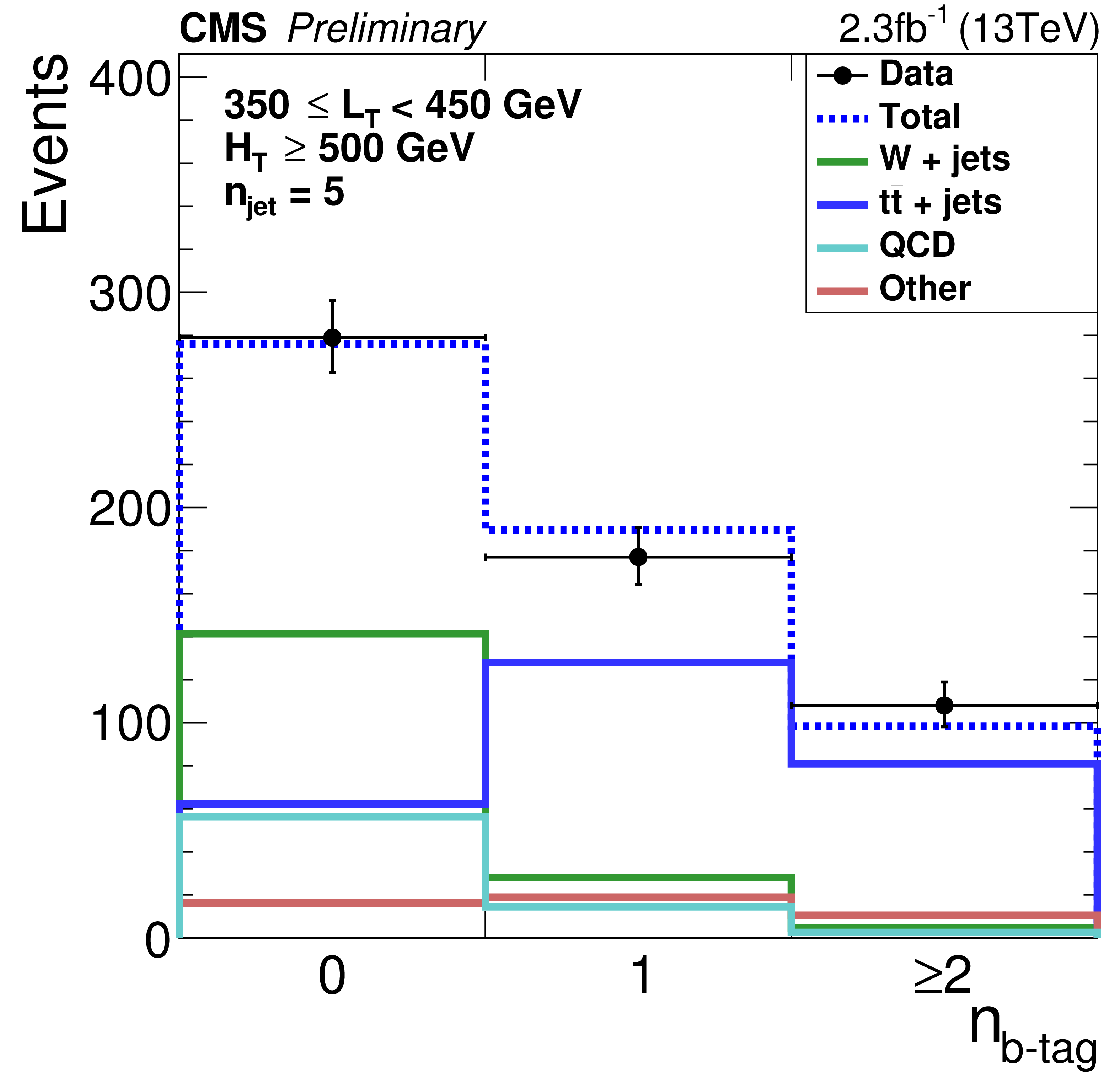
Auxiliary Figure 20:
Fits to the $ {n_\textrm {b-tag}} $ multiplicity for the control region with exactly five jets (350 $ \leq {L_{\textrm T}} <$ 450 GeV, $ {H_{\mathrm {T}}} \geq $ 500 GeV, $ {\Delta \Phi } <$ 1) in data. The solid lines represent the templates scaled according to the fit result (blue for $ {\mathrm{ t \bar{t} } } $, green for W+jets , turquoise for QCD and red for the remaining backgrounds), the dashed line shows the sum after fit, and the markers represent data. |

png pdf |
Auxiliary Figure 21:
Fits to the $ {n_\textrm {b-tag}} $ multiplicity for the control region with eight and more jets ($ {L_{\textrm T}} \geq$ 450 GeV, $ {H_{\mathrm {T}}} \geq$ 500 GeV, $ {\Delta \Phi } <$ 0.75) in data. The solid lines represent the templates scaled according to the fit result (blue for $ {\mathrm{ t \bar{t} } } $, green for W+jets , turquoise for QCD and red for the remaining backgrounds), the dashed line shows the sum after fit, and the markers represent data. |
png pdf |
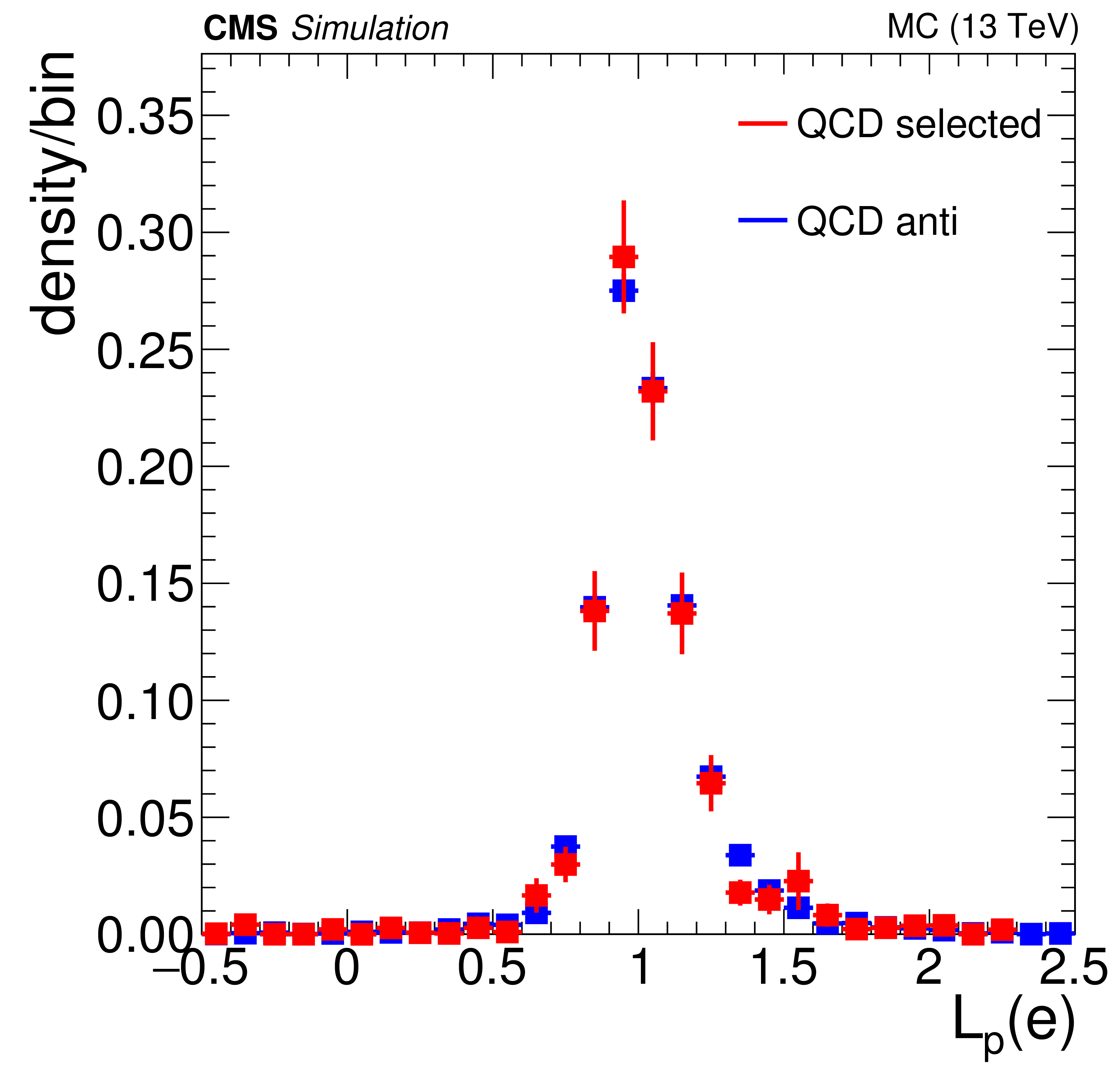
Auxiliary Figure 22:
Shapes of $ {L_{\textrm P}} $ for selected and anti-selected electrons from QCD events in simulation for $ {L_{\textrm T}} >$ 250 GeV, $ {n_\textrm {b-tag}} =$ 0, and $ {n_\textrm {jet}} $ in [3,4]. |
png pdf |
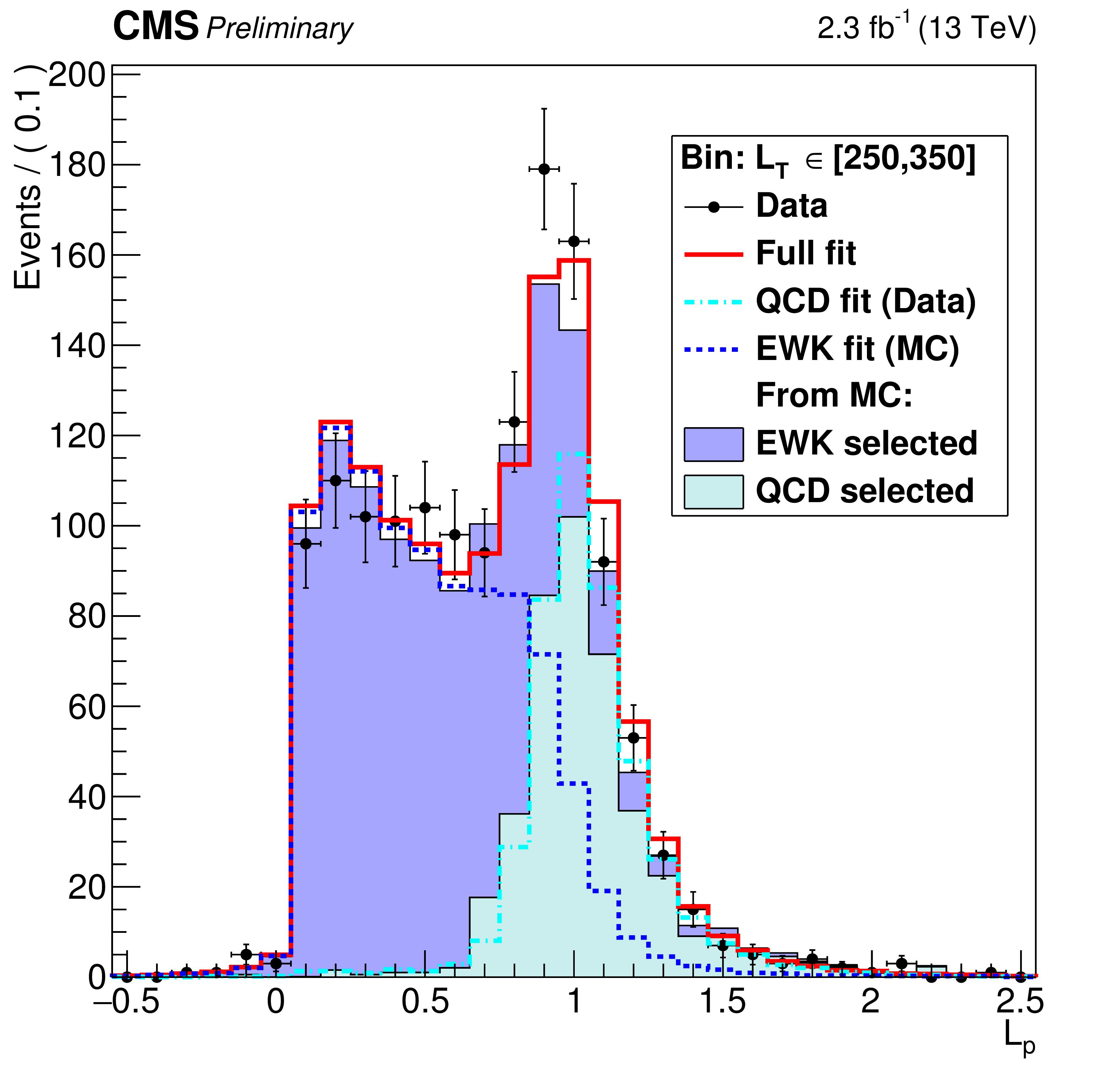
Auxiliary Figure 23:
Fit results for $ {n_\textrm {jet}}$ in [3, 4], $ {n_\textrm {b-tag}} =$ 0, and $ {L_{\textrm T}}$ in [250,350] GeV. The black dots represent data. EWK and QCD selected events from simulation normalized to the luminosity are shown with the blue and cyan filled histograms. The full fit result is shown with the solid red line, while the separate EWK and QCD components are depicted by the blue dashed and cyan dotted-dashed line, respectively. |

png pdf |
Auxiliary Figure 24:
Ratio of selected to anti-selected electron events from QCD for $ {n_\textrm {jet}} $ in [3, 4], $ {n_\textrm {b-tag}} =$ 0, in bins of $ {L_{\textrm T}} $ in data. The number of selected electrons from QCD events is extracted from the fit of the $ {L_{\textrm P}} $ distribution. |
|
|
Compact Muon Solenoid LHC, CERN |
|

|

|

|

|

|