

Compact Muon Solenoid
LHC, CERN
| CMS-PAS-HIG-15-010 | ||
| Measurement of the transverse momentum spectrum of the Higgs boson produced in pp collisions at $\sqrt{s} =$ 8 TeV using the $ \mathrm{ H \to WW } $ decays | ||
| CMS Collaboration | ||
| December 2015 | ||
| Abstract: Differential and integrated fiducial cross sections for the Higgs boson production are measured using the $\mathrm{H} \to \mathrm{W}^+ \mathrm{W}^-$ leptonic decays with an oppositely charged electron-muon pair and a pair of neutrinos in the final state. The measurements are performed using pp collisions at a centre-of-mass energy of 8 TeV collected by the CMS experiment at the LHC. Collision data correspond to an integrated luminosity of 19.4 fb$^{-1}$. The Higgs boson transverse momentum is reconstructed using the lepton pair transverse momentum and missing transverse momentum, which originates from the presence of two neutrinos in the final state. The differential cross section is measured as a function of the Higgs boson transverse momentum in a fiducial phase space defined to match the experimental acceptance in terms of the lepton kinematics and event topology. The inclusive production cross section times branching fraction in the fiducial phase space is measured to be 39 $\pm$ 8 (stat) $\pm$ 9 (syst) fb. The measurements are compared to theoretical calculations based on the standard model, and found to be in agreement with them within the experimental uncertainties. | ||
|
Links:
CDS record (PDF) ;
Public twiki page ;
CADI line (restricted) ;
These preliminary results are superseded in this paper, JHEP 03 (2017) 032. The superseded preliminary plots can be found here. |
||
| Figures | |
png ; pdf ; |
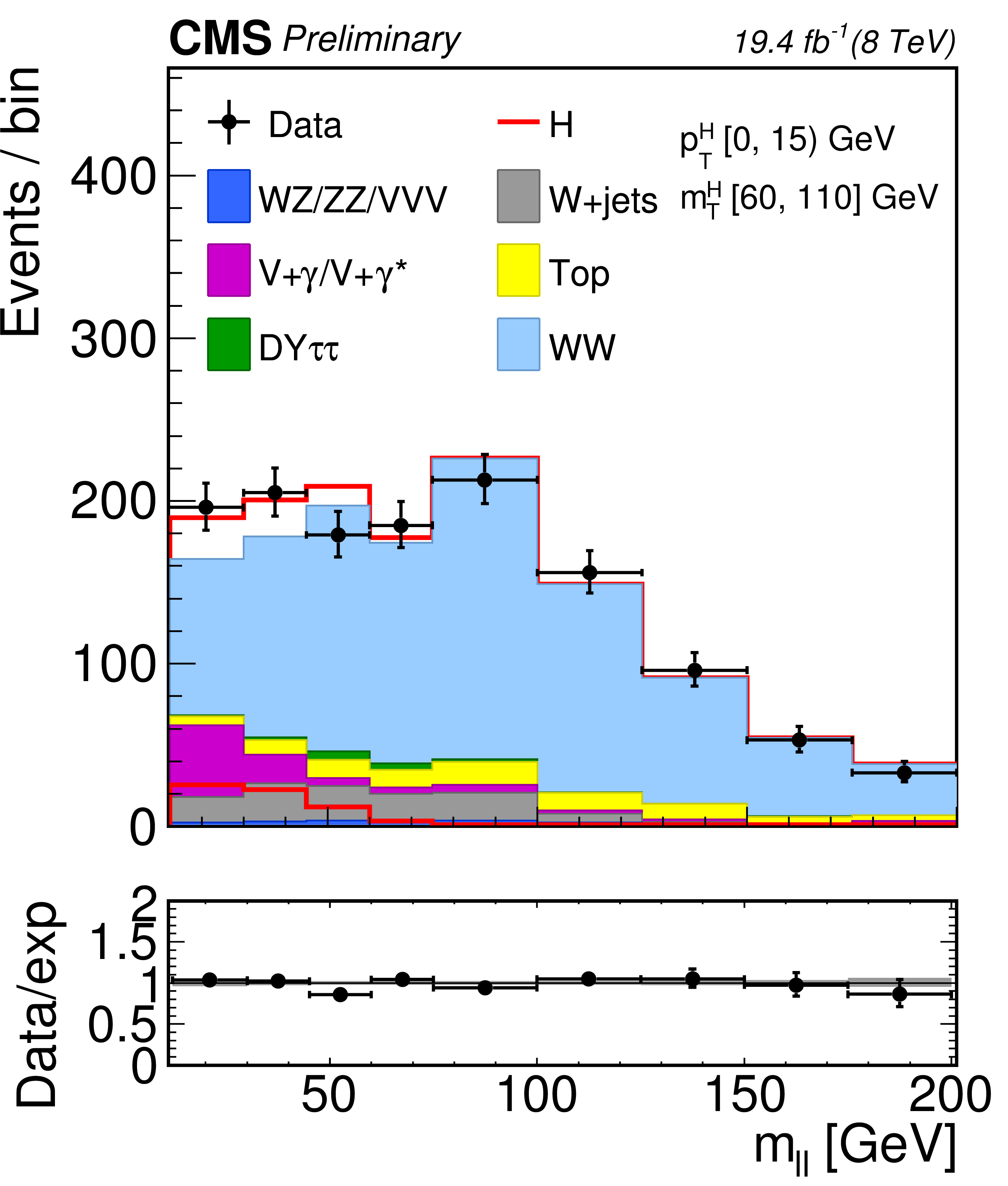
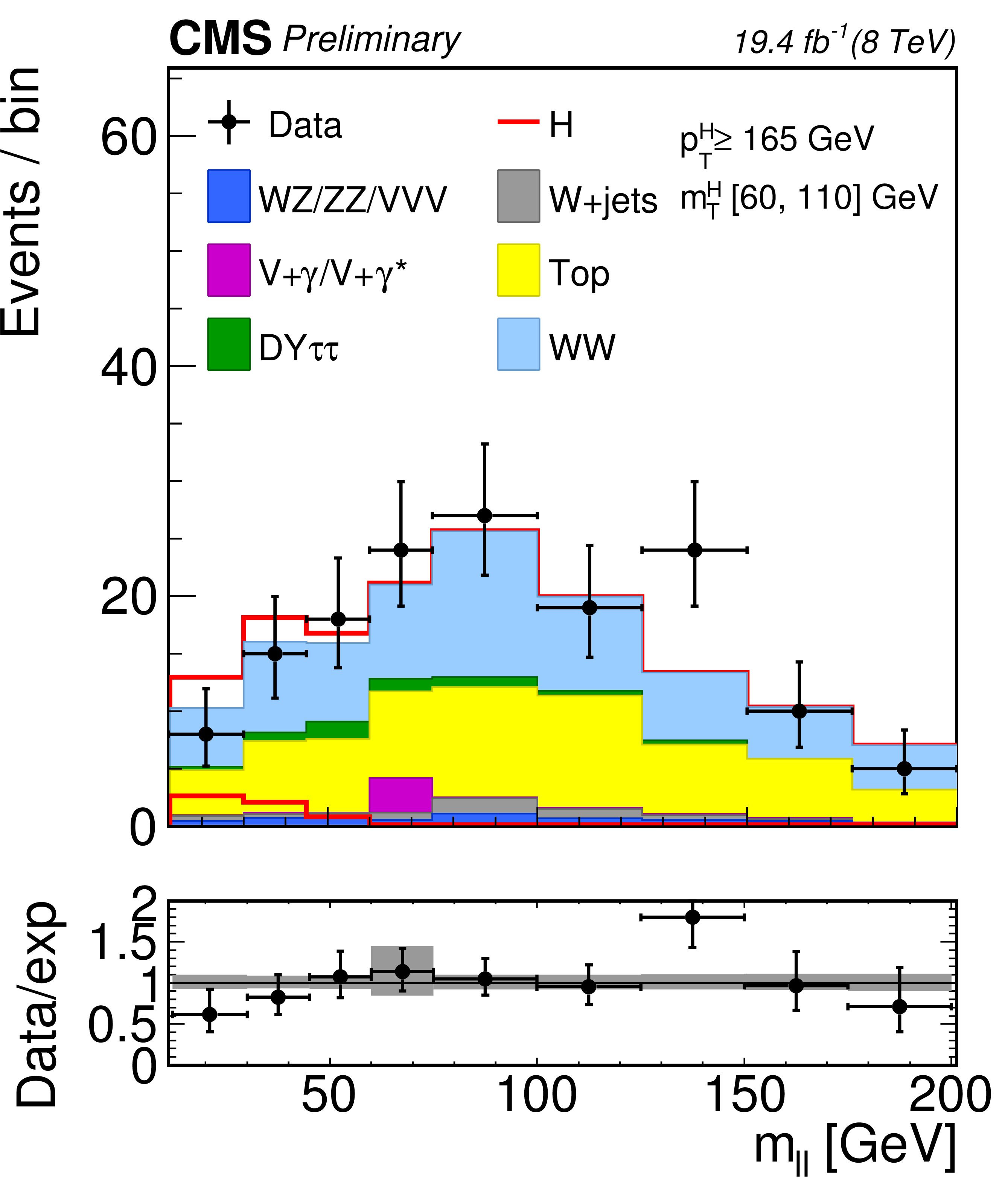
Figure 1-a:
Distributions of the $ {m_{ {\ell } {\ell }}} $ variable in every Higgs boson $ {p_{\mathrm {T}}} $ bin. Background normalizations correspond to the values obtained from the fit. Signal normalization is fixed to the MC expectation. The distributions are shown in a $ {m_{\mathrm {T}}^{\ell \ell {E_{\mathrm {T}}^{\text {miss}}} }}$ window of [60,110] GeV in order to emphasize the Higgs boson (H) signal. Ratios of the expected and observed event yields in individual bins are shown in the panels below the plots. |
png ; pdf ; |
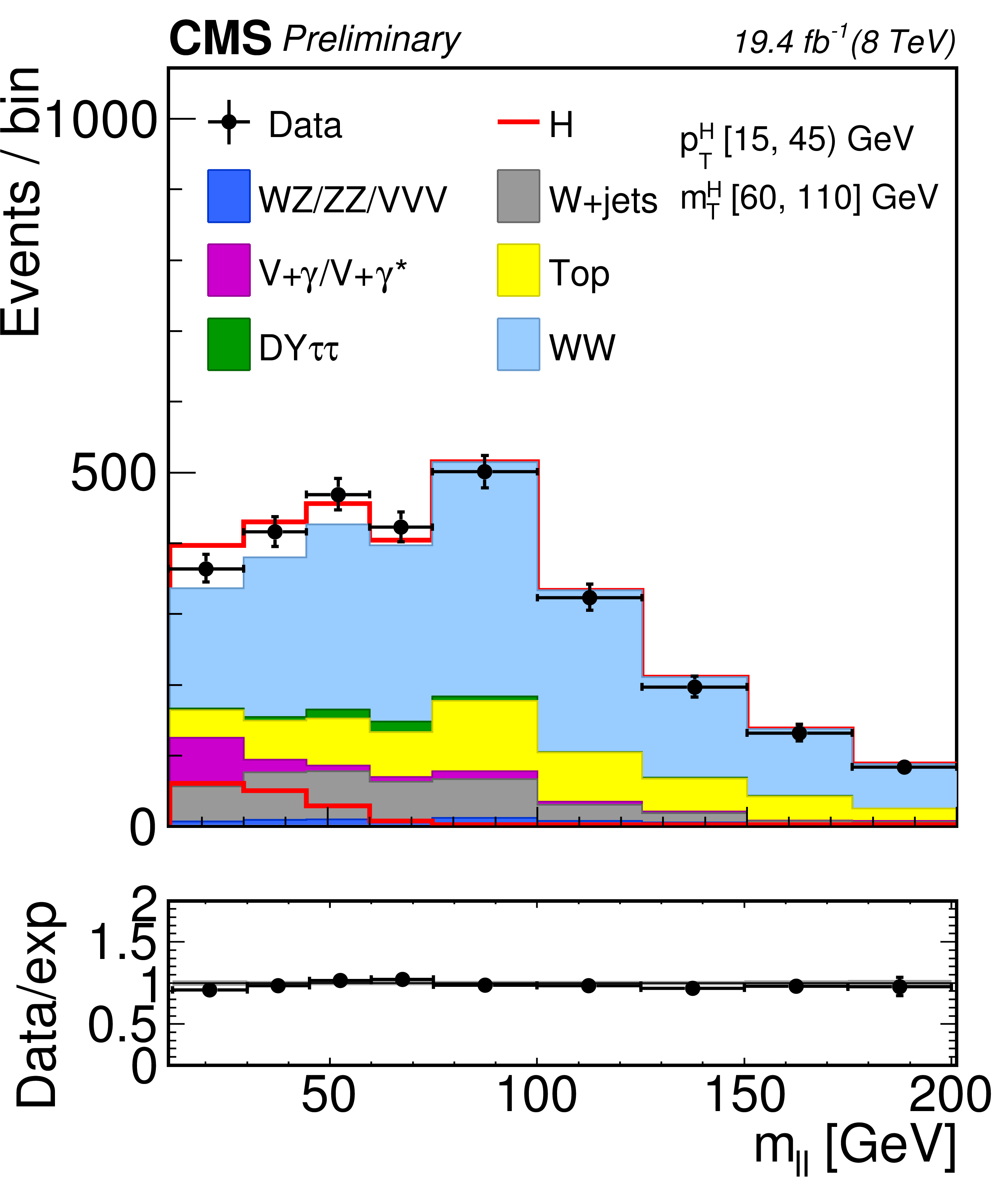
Figure 1-b:
Distributions of the $ {m_{ {\ell } {\ell }}} $ variable in every Higgs boson $ {p_{\mathrm {T}}} $ bin. Background normalizations correspond to the values obtained from the fit. Signal normalization is fixed to the MC expectation. The distributions are shown in a $ {m_{\mathrm {T}}^{\ell \ell {E_{\mathrm {T}}^{\text {miss}}} }}$ window of [60,110] GeV in order to emphasize the Higgs boson (H) signal. Ratios of the expected and observed event yields in individual bins are shown in the panels below the plots. |
png ; pdf ; |
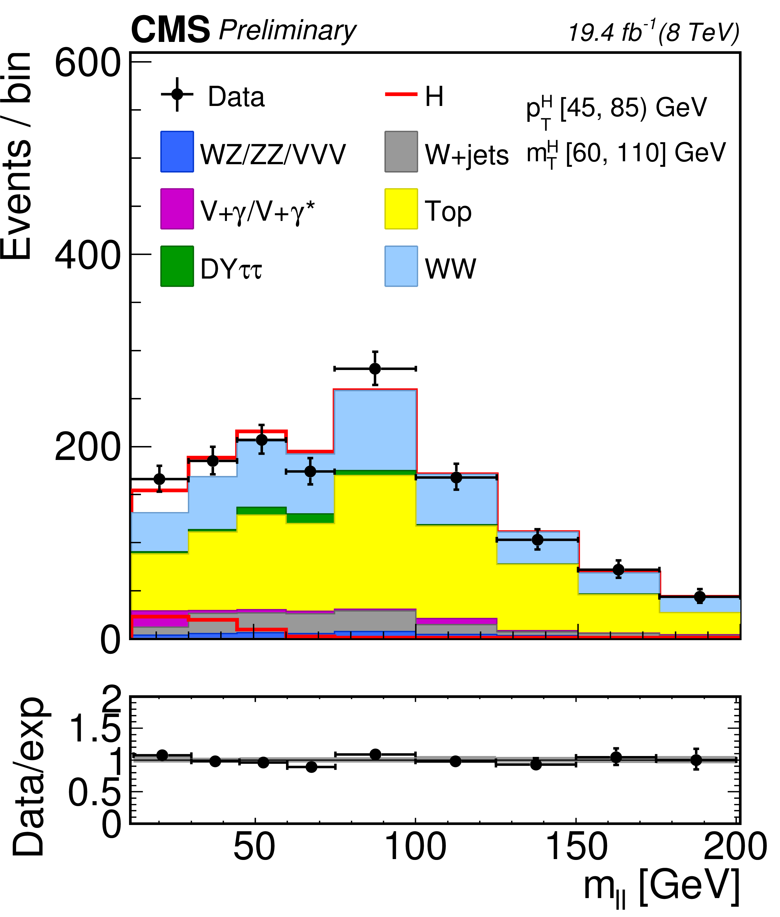
Figure 1-c:
Distributions of the $ {m_{ {\ell } {\ell }}} $ variable in every Higgs boson $ {p_{\mathrm {T}}} $ bin. Background normalizations correspond to the values obtained from the fit. Signal normalization is fixed to the MC expectation. The distributions are shown in a $ {m_{\mathrm {T}}^{\ell \ell {E_{\mathrm {T}}^{\text {miss}}} }}$ window of [60,110] GeV in order to emphasize the Higgs boson (H) signal. Ratios of the expected and observed event yields in individual bins are shown in the panels below the plots. |

png ; pdf ; |
Figure 1-d:
Distributions of the $ {m_{ {\ell } {\ell }}} $ variable in every Higgs boson $ {p_{\mathrm {T}}} $ bin. Background normalizations correspond to the values obtained from the fit. Signal normalization is fixed to the MC expectation. The distributions are shown in a $ {m_{\mathrm {T}}^{\ell \ell {E_{\mathrm {T}}^{\text {miss}}} }}$ window of [60,110] GeV in order to emphasize the Higgs boson (H) signal. Ratios of the expected and observed event yields in individual bins are shown in the panels below the plots. |
png ; pdf ; |
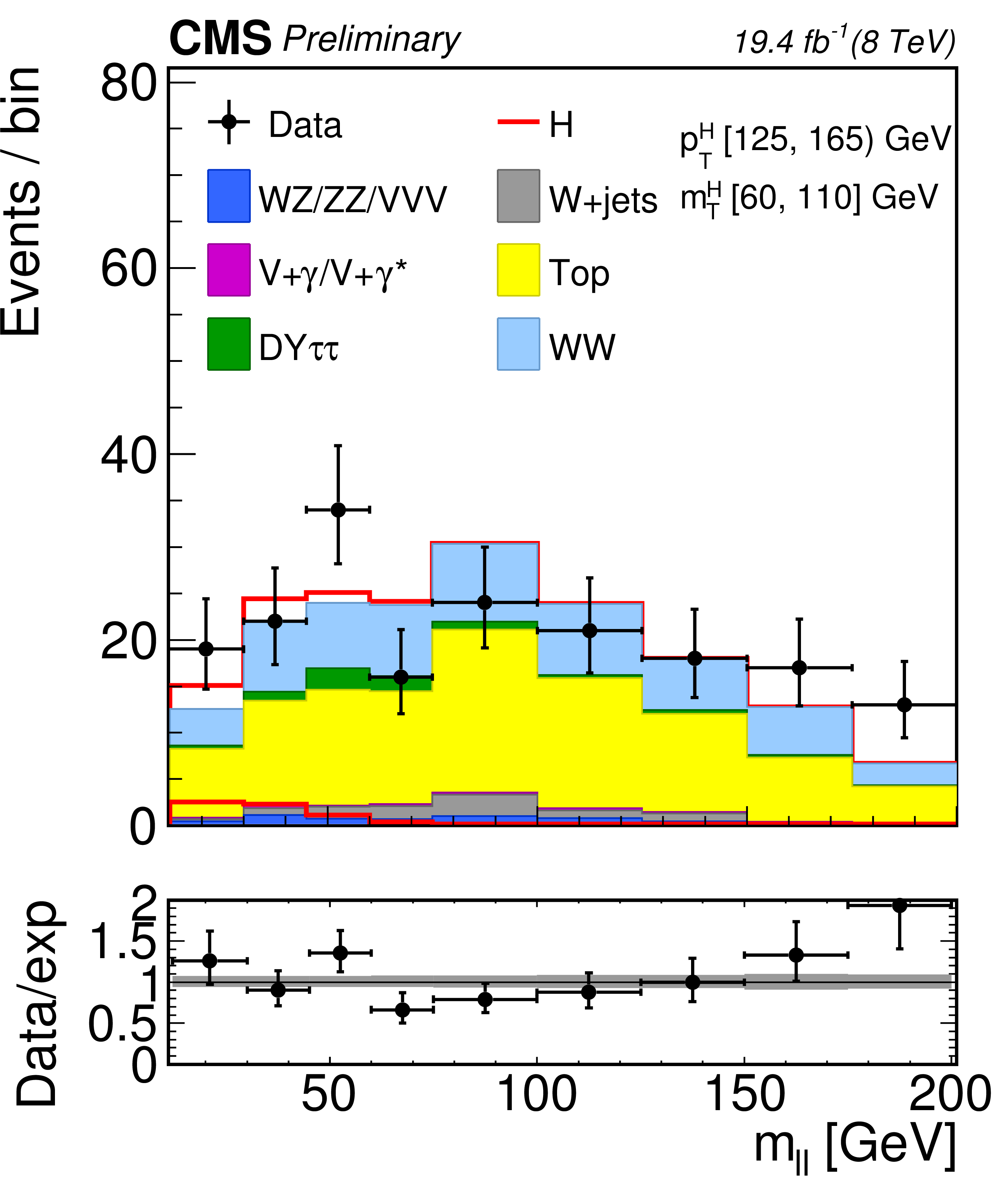
Figure 1-e:
Distributions of the $ {m_{ {\ell } {\ell }}} $ variable in every Higgs boson $ {p_{\mathrm {T}}} $ bin. Background normalizations correspond to the values obtained from the fit. Signal normalization is fixed to the MC expectation. The distributions are shown in a $ {m_{\mathrm {T}}^{\ell \ell {E_{\mathrm {T}}^{\text {miss}}} }}$ window of [60,110] GeV in order to emphasize the Higgs boson (H) signal. Ratios of the expected and observed event yields in individual bins are shown in the panels below the plots. |
png ; pdf ; |
Figure 1-f:
Distributions of the $ {m_{ {\ell } {\ell }}} $ variable in every Higgs boson $ {p_{\mathrm {T}}} $ bin. Background normalizations correspond to the values obtained from the fit. Signal normalization is fixed to the MC expectation. The distributions are shown in a $ {m_{\mathrm {T}}^{\ell \ell {E_{\mathrm {T}}^{\text {miss}}} }}$ window of [60,110] GeV in order to emphasize the Higgs boson (H) signal. Ratios of the expected and observed event yields in individual bins are shown in the panels below the plots. |

png ; pdf ; |
Figure 2:
Differential Higgs boson production cross section as a function of reconstructed Higgs boson $ {p_{\mathrm {T}}} $, before applying the unfolding procedure. Data values are shown together with the statistical (azure band) and the systematic (gray band) uncertainties. The green line and dashed area represent the SM theoretical estimates in which the acceptance of the dominant $\mathrm{ gg \to H $ contribution is modelled by Powheg 1.0 (PowhegV1). The sub-dominant component of the signal is denoted as XH=VBF+VH and it is also shown separately. |
png ; pdf ; |
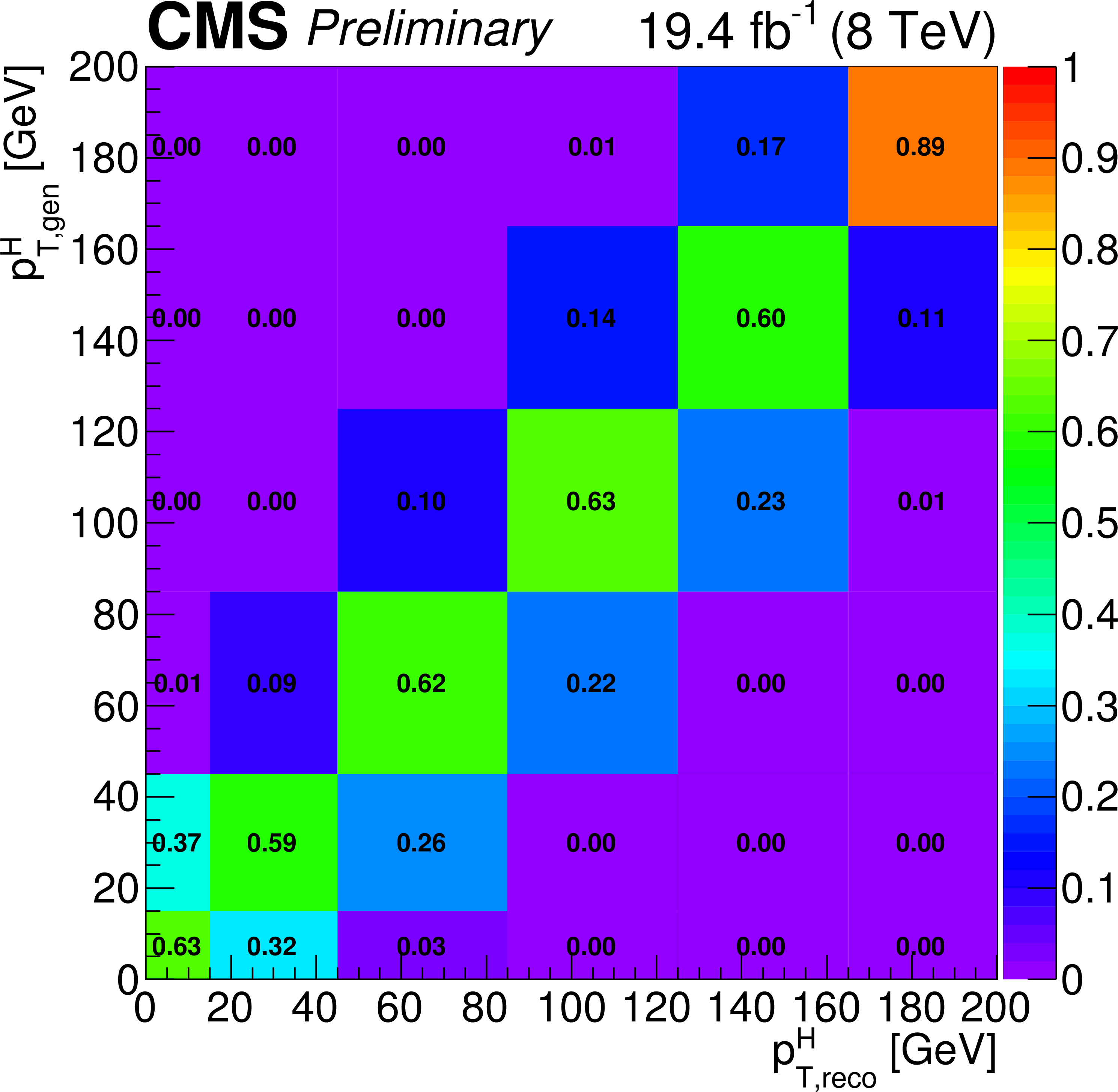
Figure 3-a:
Deconvolution matrix (a) and response matrix (b) including all signal processes. The matrices were normalized either by column (a) or by row (b) in order to show the purity or stability respectively in diagonal bins. |

png ; pdf ; |
Figure 3-b:
Deconvolution matrix (a) and response matrix (b) including all signal processes. The matrices were normalized either by column (a) or by row (b) in order to show the purity or stability respectively in diagonal bins. |

png ; pdf ; |
Figure 4:
Differential Higgs boson production cross section as a function of Higgs boson $ {p_{\mathrm {T}}} $, after applying the unfolding procedure. Unfolded data values are shown, together with statistical uncertainty (azure band) and systematic uncertainty (gray band). The vertical bars on the data points correspond to the sum in quadrature of the statistical and systematic uncertainties. The model dependence uncertainty is also shown (red band). The pink and green lines and dashed areas represent the SM theoretical estimates in which the acceptance of the dominant $ \mathrm{ gg \to H } $ contribution is modeled by HRes and Powheg 2.0 (PowhegV2) respectively. The sub-dominant component of the signal is denoted as XH=VBF+VH and it is also shown separately. |
|
|
Compact Muon Solenoid LHC, CERN |
|

|

|

|

|

|