

Compact Muon Solenoid
LHC, CERN
| CMS-PAS-HIG-14-040 | ||
| Search for lepton-flavour-violating decays of the Higgs boson to $\mathrm{ e \tau } $ and $\mathrm{ e \mu } $ at $ \sqrt{s} = $ 8 TeV | ||
| CMS Collaboration | ||
| August 2015 | ||
| Abstract: A direct search for lepton-flavour-violating decays of a Higgs boson ($m_{\mathrm{H}} =$ 125 GeV) is described. The search is performed for the $\mathrm{H} \rightarrow \mathrm{e} \tau_{\mu}$, $\textrm{H} \rightarrow \mathrm{e} \tau_{h}$, and $\mathrm{H} \rightarrow \mathrm{e} \mu$ decays, where $\tau_{h}$ and $\tau_{\mu}$ are taus reconstructed in the hadronic and muonic decay channels, respectively. The data sample used in the search corresponds to an integrated luminosity of 19.7 fb$^{-1}$ collected in pp collisions at $ \sqrt{s}= $ 8 TeV with the CMS experiment at the CERN LHC. No evidence is found for lepton-flavour-violating decays in either final state. For the $\mathrm{H} \rightarrow \mathrm{e} \tau_{\mu}$ and $\mathrm{H} \rightarrow \mathrm{e} \tau_{h}$ channels, the sensitivity of the search is an order of magnitude better than the existing indirect limits. A constraint of $\mathcal{B}(\mathrm{H} \rightarrow \mathrm{e} \tau )<$ 0.70% at 95% confidence level is set. We also set a limit on the branching ratio of $\mathcal{B}(\mathrm{H} \rightarrow \mathrm{e} \mu) <$ 0.036% at 95% confidence level. The limits on $\mathcal{B}(\mathrm{H} \rightarrow \mathrm{e} \tau )$ and $\mathcal{B}(\mathrm{H} \rightarrow \mathrm{e} \mu)$ are subsequently used to constrain the $|Y_{\mathrm{e}\tau}|$ and $|Y_{\mathrm{e}\mu}|$ Yukawa couplings. | ||
|
Links:
CDS record (PDF) ;
CADI line (restricted) ; Figures are also available from the CDS record. These preliminary results are superseded in this paper, PLB 763C (2016) 472. The superseded preliminary plots can be found here. |
||
| Figures | |
png ; pdf |
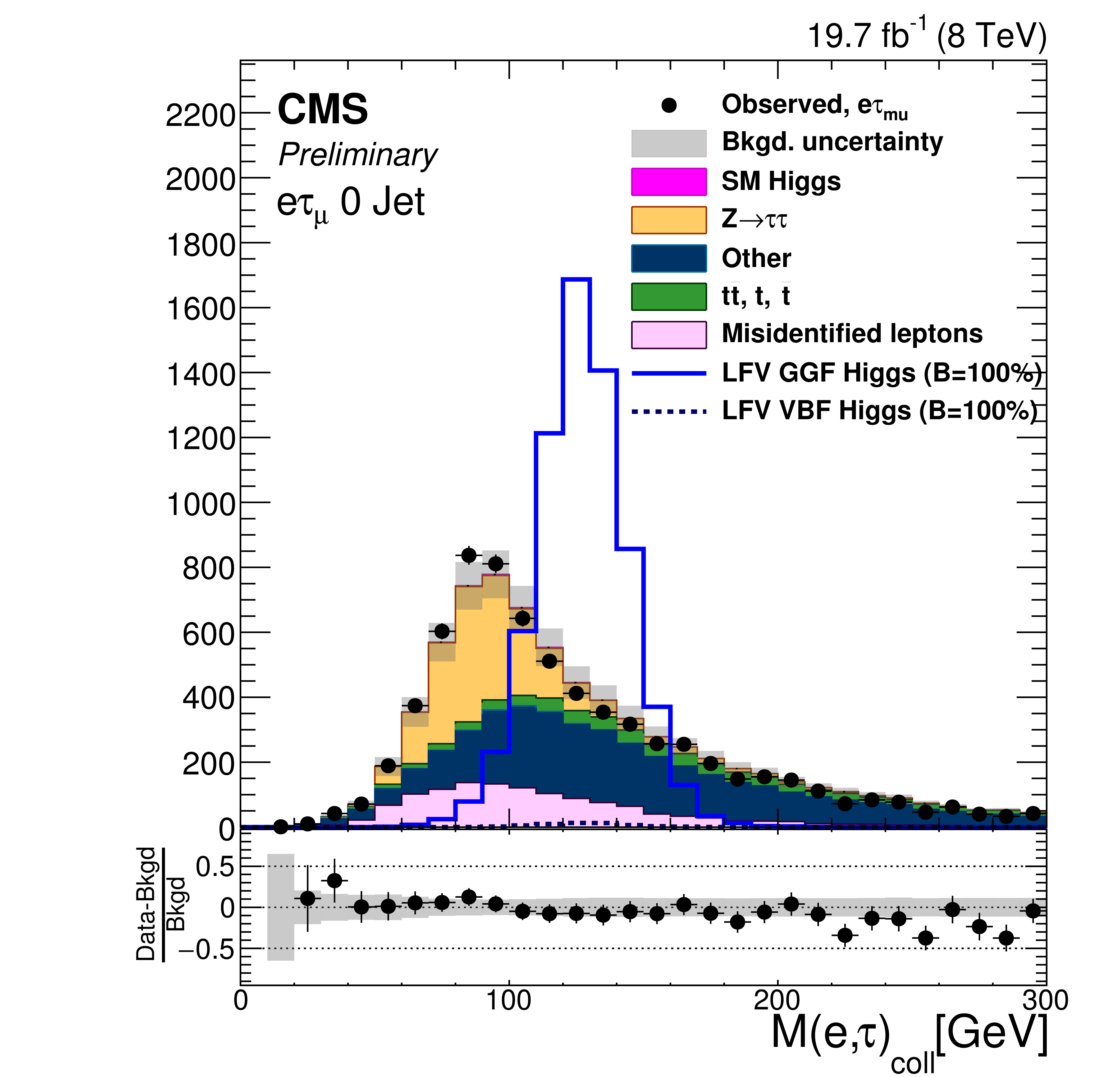
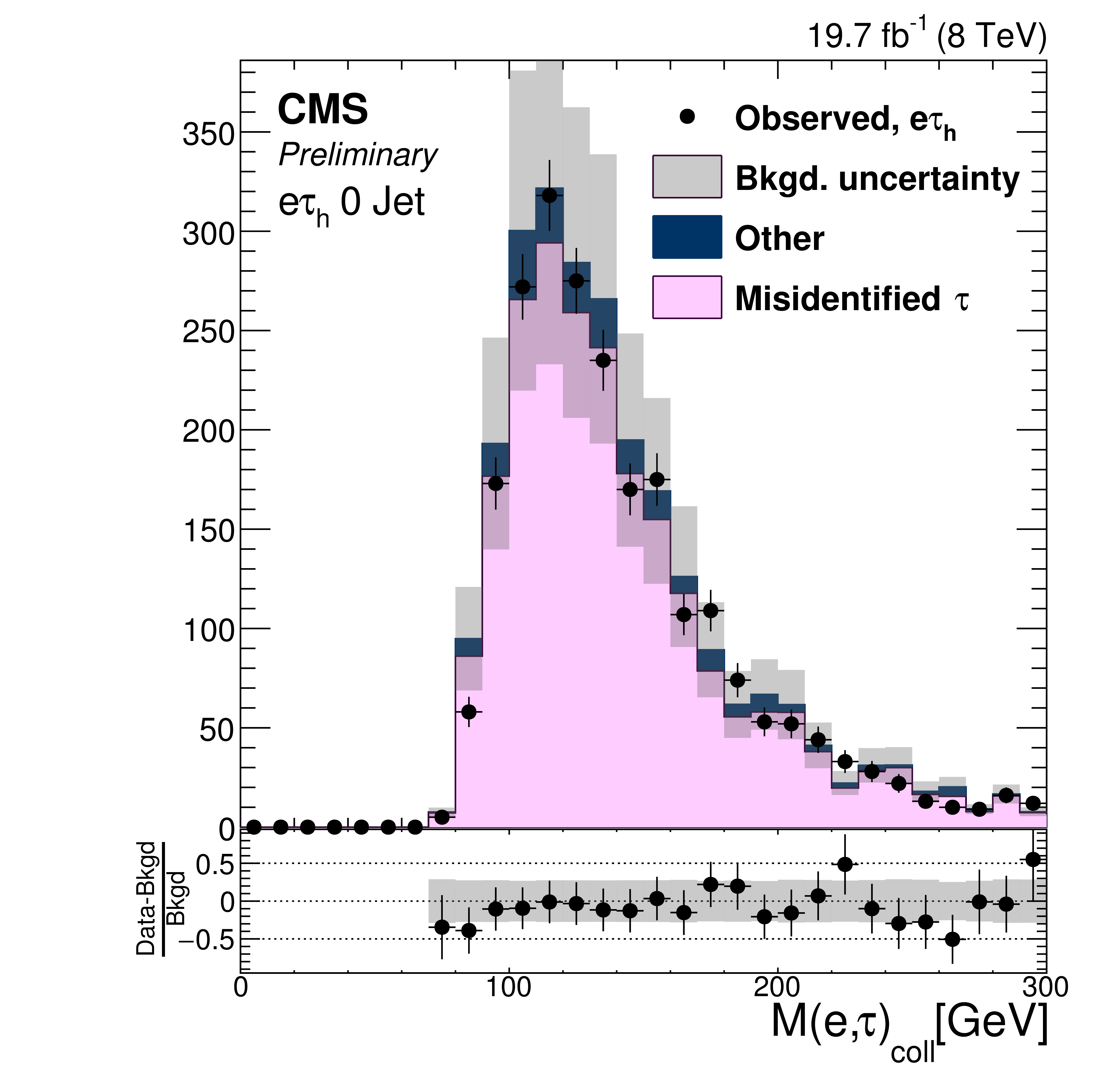
Figure 1-a:
Comparison of the observed collinear mass distributions with the background expectations after the loose selection requirements. The shaded gray bands indicate the total uncertainty. The expected distributions for signal with $B( {\mathrm {H}} \to {\mathrm {e}} {\tau })=$ 100% are shown for clarity. a: $ {\mathrm {H}} \to {\mathrm {e}} {\tau }_{ {{\mu }}}$ 0-jet; b: $ {\mathrm {H}} \to {\mathrm {e}} {\tau }_{h}$ 0-jet; c: $ {\mathrm {H}} \to {\mathrm {e}} {\tau }_{ {{\mu }}}$ 1-jet; d: $ {\mathrm {H}} \to {\mathrm {e}} {\tau }_{h}$1-jet; e: $ {\mathrm {H}} \to {\mathrm {e}} {\tau }_{ {{\mu }}}$ 2-jet; f: $ {\mathrm {H}} \to {\mathrm {e}} {\tau }_{h}$ 2-jet. |

png ; pdf |
Figure 1-b:
Comparison of the observed collinear mass distributions with the background expectations after the loose selection requirements. The shaded gray bands indicate the total uncertainty. The expected distributions for signal with $B( {\mathrm {H}} \to {\mathrm {e}} {\tau })=$ 100% are shown for clarity. a: $ {\mathrm {H}} \to {\mathrm {e}} {\tau }_{ {{\mu }}}$ 0-jet; b: $ {\mathrm {H}} \to {\mathrm {e}} {\tau }_{h}$ 0-jet; c: $ {\mathrm {H}} \to {\mathrm {e}} {\tau }_{ {{\mu }}}$ 1-jet; d: $ {\mathrm {H}} \to {\mathrm {e}} {\tau }_{h}$1-jet; e: $ {\mathrm {H}} \to {\mathrm {e}} {\tau }_{ {{\mu }}}$ 2-jet; f: $ {\mathrm {H}} \to {\mathrm {e}} {\tau }_{h}$ 2-jet. |

png ; pdf |
Figure 1-c:
Comparison of the observed collinear mass distributions with the background expectations after the loose selection requirements. The shaded gray bands indicate the total uncertainty. The expected distributions for signal with $B( {\mathrm {H}} \to {\mathrm {e}} {\tau })=$ 100% are shown for clarity. a: $ {\mathrm {H}} \to {\mathrm {e}} {\tau }_{ {{\mu }}}$ 0-jet; b: $ {\mathrm {H}} \to {\mathrm {e}} {\tau }_{h}$ 0-jet; c: $ {\mathrm {H}} \to {\mathrm {e}} {\tau }_{ {{\mu }}}$ 1-jet; d: $ {\mathrm {H}} \to {\mathrm {e}} {\tau }_{h}$1-jet; e: $ {\mathrm {H}} \to {\mathrm {e}} {\tau }_{ {{\mu }}}$ 2-jet; f: $ {\mathrm {H}} \to {\mathrm {e}} {\tau }_{h}$ 2-jet. |
png ; pdf |
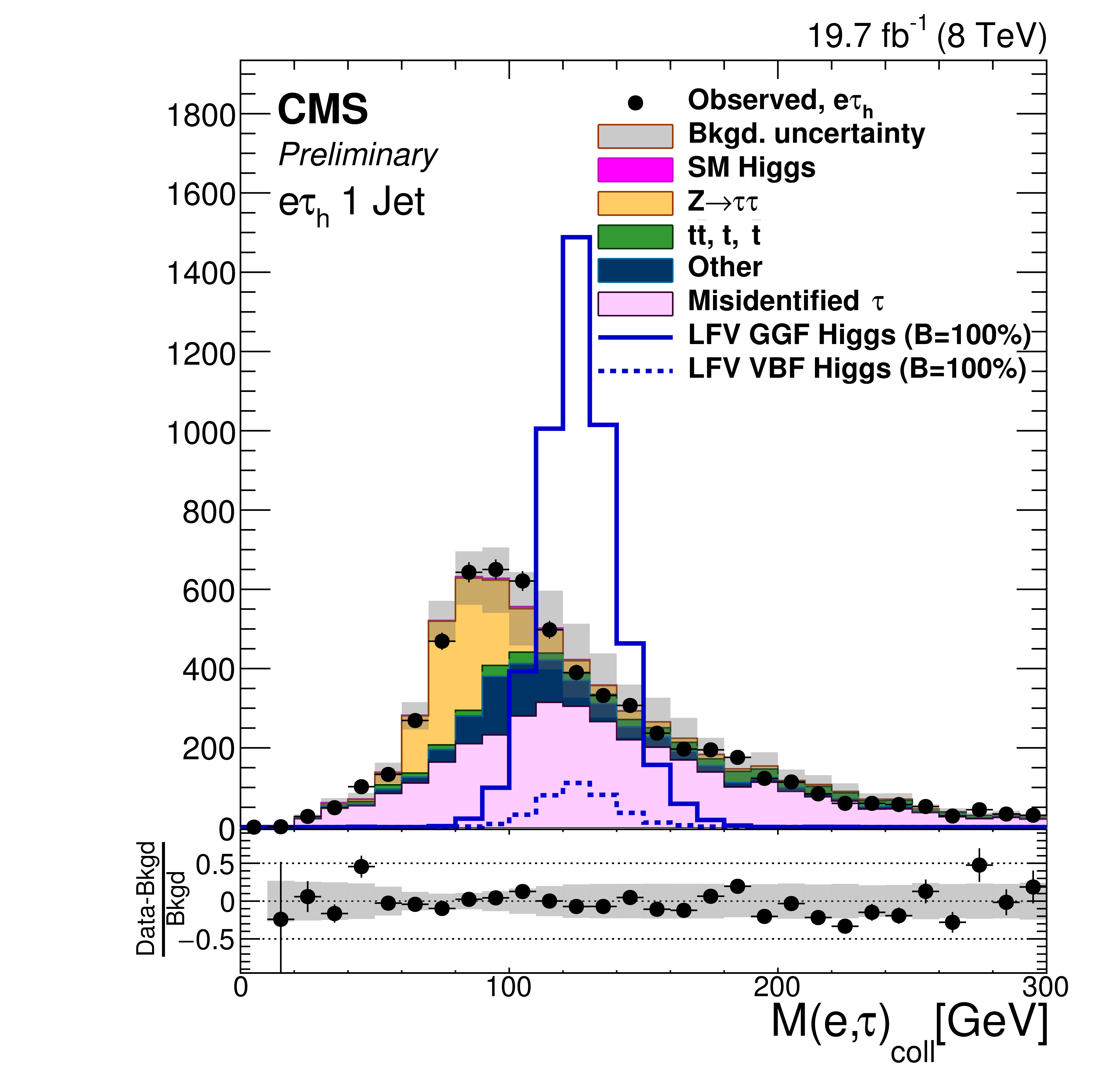
Figure 1-d:
Comparison of the observed collinear mass distributions with the background expectations after the loose selection requirements. The shaded gray bands indicate the total uncertainty. The expected distributions for signal with $B( {\mathrm {H}} \to {\mathrm {e}} {\tau })=$ 100% are shown for clarity. a: $ {\mathrm {H}} \to {\mathrm {e}} {\tau }_{ {{\mu }}}$ 0-jet; b: $ {\mathrm {H}} \to {\mathrm {e}} {\tau }_{h}$ 0-jet; c: $ {\mathrm {H}} \to {\mathrm {e}} {\tau }_{ {{\mu }}}$ 1-jet; d: $ {\mathrm {H}} \to {\mathrm {e}} {\tau }_{h}$1-jet; e: $ {\mathrm {H}} \to {\mathrm {e}} {\tau }_{ {{\mu }}}$ 2-jet; f: $ {\mathrm {H}} \to {\mathrm {e}} {\tau }_{h}$ 2-jet. |

png ; pdf |
Figure 1-e:
Comparison of the observed collinear mass distributions with the background expectations after the loose selection requirements. The shaded gray bands indicate the total uncertainty. The expected distributions for signal with $B( {\mathrm {H}} \to {\mathrm {e}} {\tau })=$ 100% are shown for clarity. a: $ {\mathrm {H}} \to {\mathrm {e}} {\tau }_{ {{\mu }}}$ 0-jet; b: $ {\mathrm {H}} \to {\mathrm {e}} {\tau }_{h}$ 0-jet; c: $ {\mathrm {H}} \to {\mathrm {e}} {\tau }_{ {{\mu }}}$ 1-jet; d: $ {\mathrm {H}} \to {\mathrm {e}} {\tau }_{h}$1-jet; e: $ {\mathrm {H}} \to {\mathrm {e}} {\tau }_{ {{\mu }}}$ 2-jet; f: $ {\mathrm {H}} \to {\mathrm {e}} {\tau }_{h}$ 2-jet. |
png ; pdf |
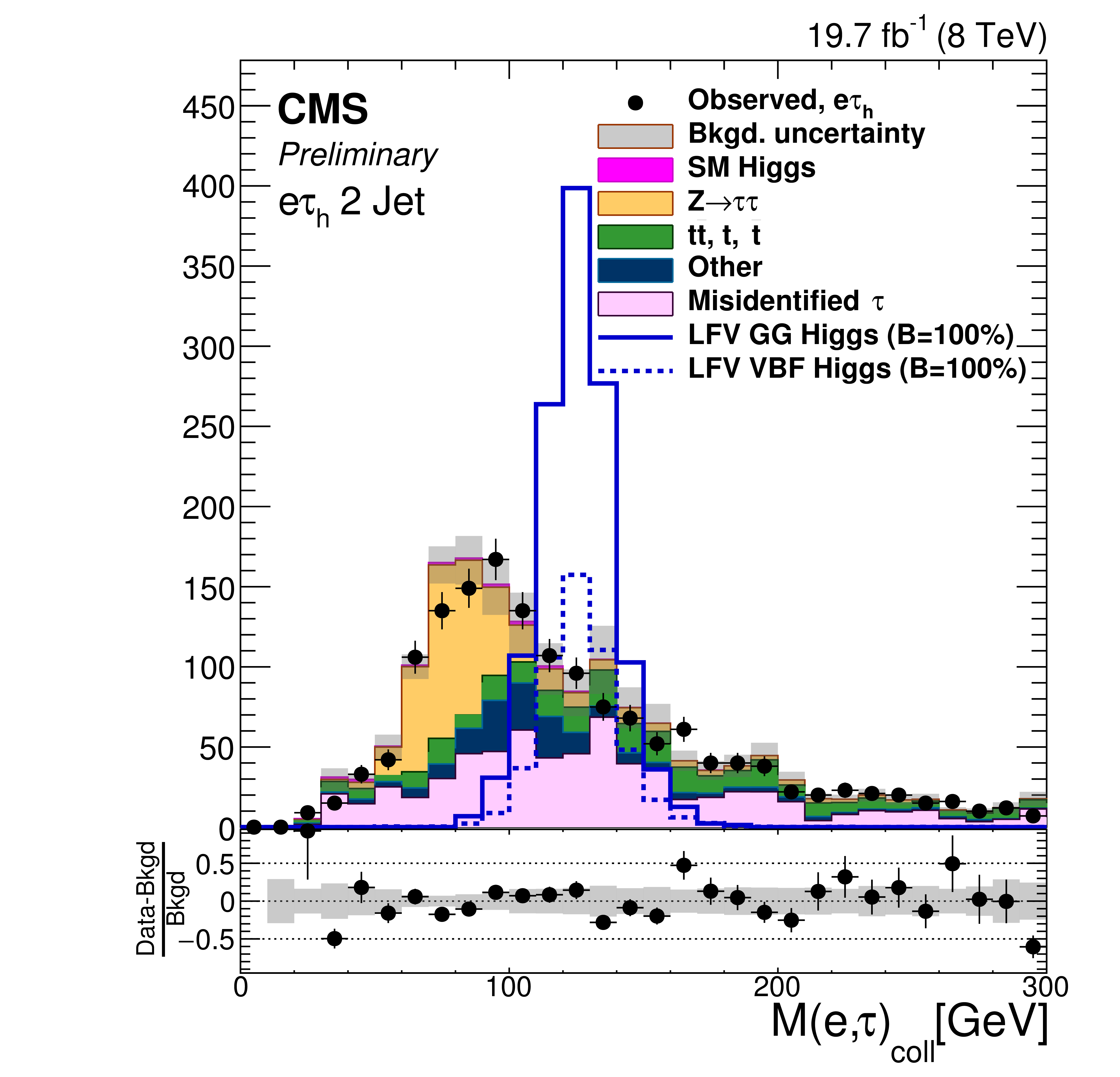
Figure 1-f:
Comparison of the observed collinear mass distributions with the background expectations after the loose selection requirements. The shaded gray bands indicate the total uncertainty. The expected distributions for signal with $B( {\mathrm {H}} \to {\mathrm {e}} {\tau })=$ 100% are shown for clarity. a: $ {\mathrm {H}} \to {\mathrm {e}} {\tau }_{ {{\mu }}}$ 0-jet; b: $ {\mathrm {H}} \to {\mathrm {e}} {\tau }_{h}$ 0-jet; c: $ {\mathrm {H}} \to {\mathrm {e}} {\tau }_{ {{\mu }}}$ 1-jet; d: $ {\mathrm {H}} \to {\mathrm {e}} {\tau }_{h}$1-jet; e: $ {\mathrm {H}} \to {\mathrm {e}} {\tau }_{ {{\mu }}}$ 2-jet; f: $ {\mathrm {H}} \to {\mathrm {e}} {\tau }_{h}$ 2-jet. |
png ; pdf |
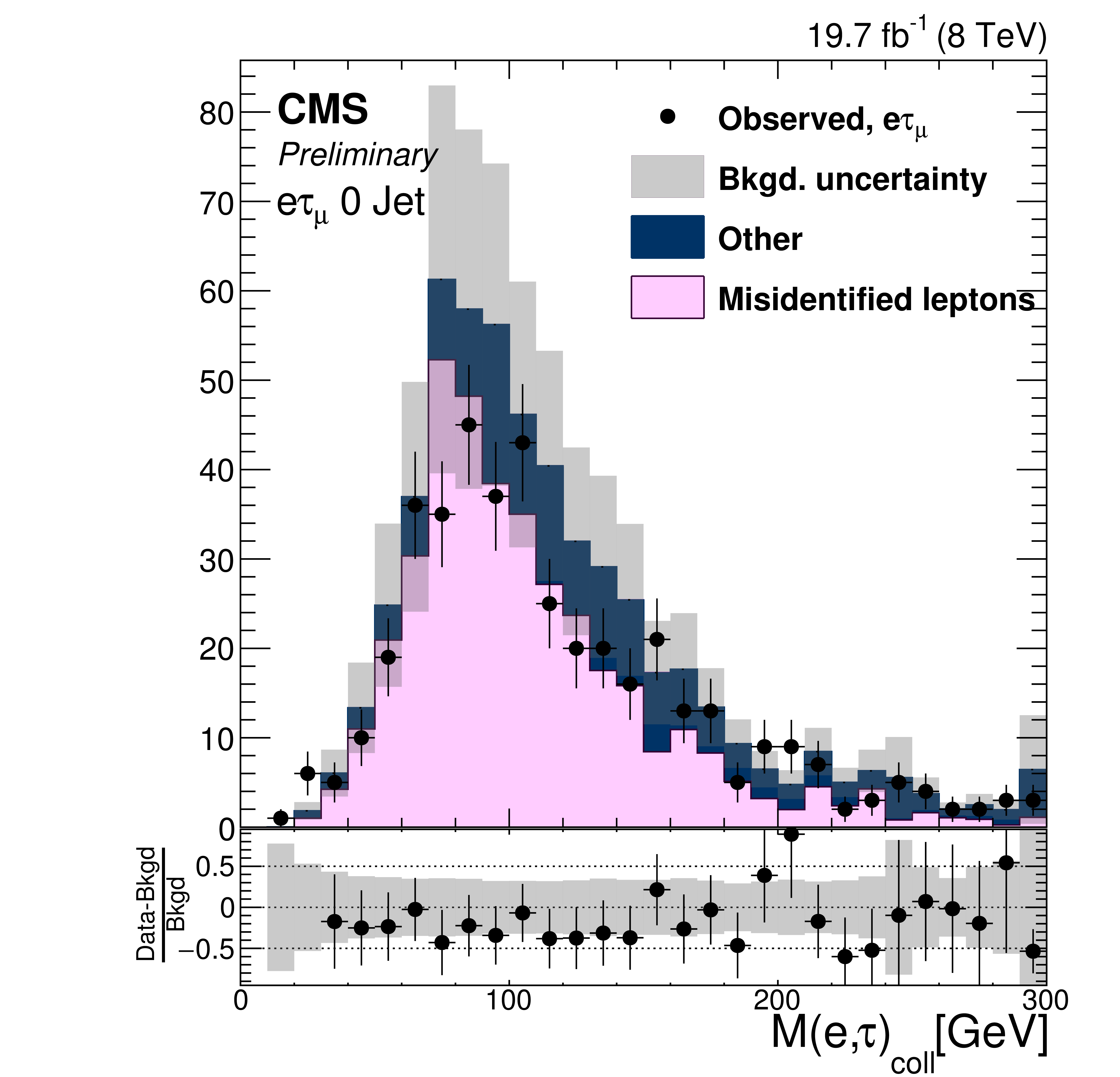
Figure 2-a:
Distributions of $\text {M}_{\text {col}}$ for region II. a: $ {\mathrm {H}} \to {\mathrm {e}} {\tau }_{ {{\mu }}}$. b: $ {\mathrm {H}} \to {\mathrm {e}} {\tau }_{h}$. |
png ; pdf |
Figure 2-b:
Distributions of $\text {M}_{\text {col}}$ for region II. a: $ {\mathrm {H}} \to {\mathrm {e}} {\tau }_{ {{\mu }}}$. b: $ {\mathrm {H}} \to {\mathrm {e}} {\tau }_{h}$. |
png ; pdf |
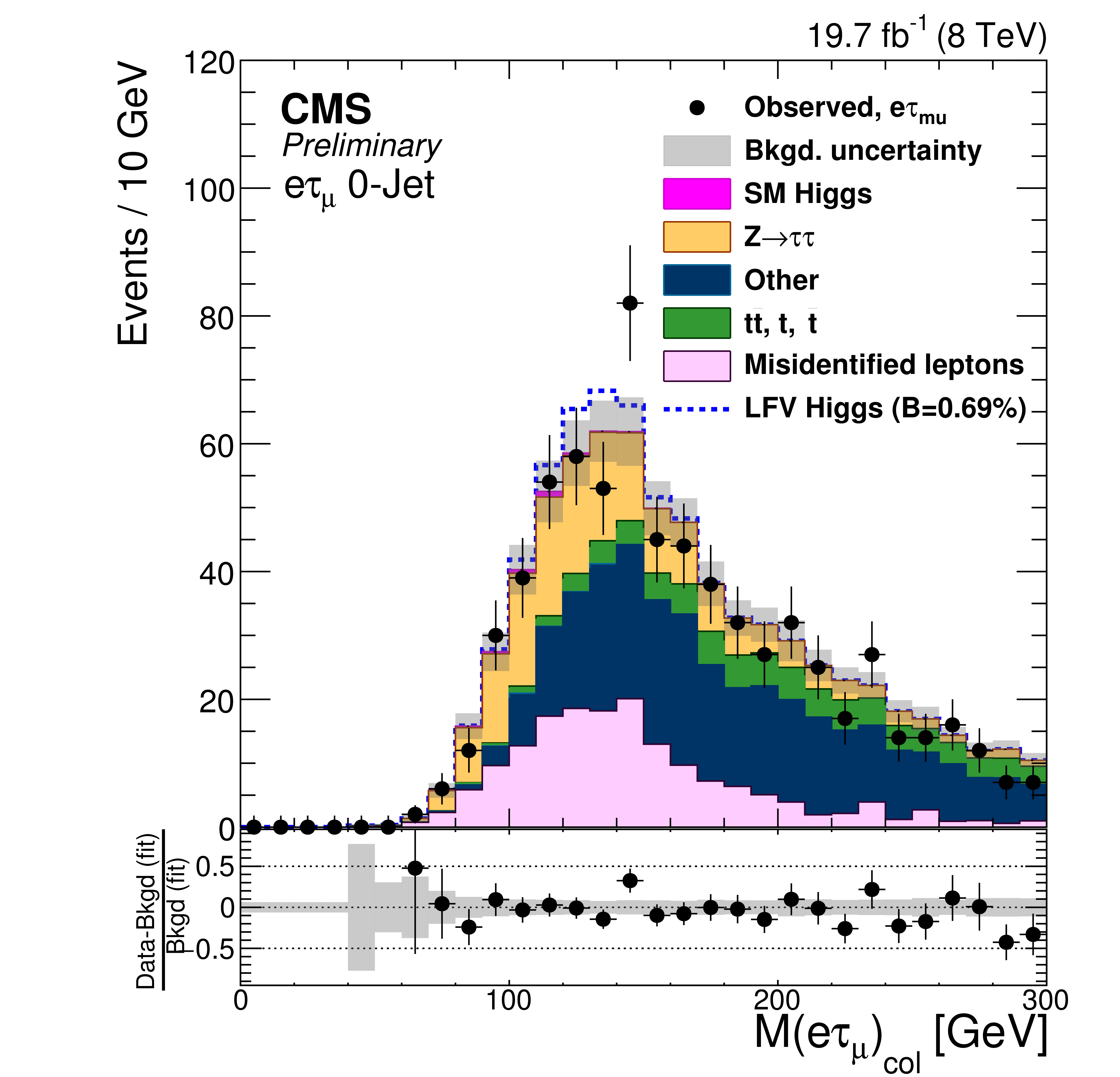
Figure 3-a:
Comparison of the observed collinear mass distributions with the background expectations after the fit. The simulated distributions for signal is shown for the branching ratio $B( {\mathrm {H}} \to {\mathrm {e}} {\tau })=0.69%$. a: $ {\mathrm {H}} \to {\mathrm {e}} {\tau }_{ {{\mu }}}$ 0-jet; b: $ {\mathrm {H}} \to {\mathrm {e}} {\tau }_{h}$ 0-jet; c: $ {\mathrm {H}} \to {\mathrm {e}} {\tau }_{ {{\mu }}}$ 1-jet; d: $ {\mathrm {H}} \to {\mathrm {e}} {\tau }_{h}$1-jet; e: $ {\mathrm {H}} \to {\mathrm {e}} {\tau }_{ {{\mu }}}$ 2-jet; f: $ {\mathrm {H}} \to {\mathrm {e}} {\tau }_{h}$ 2-jet. |
png ; pdf |
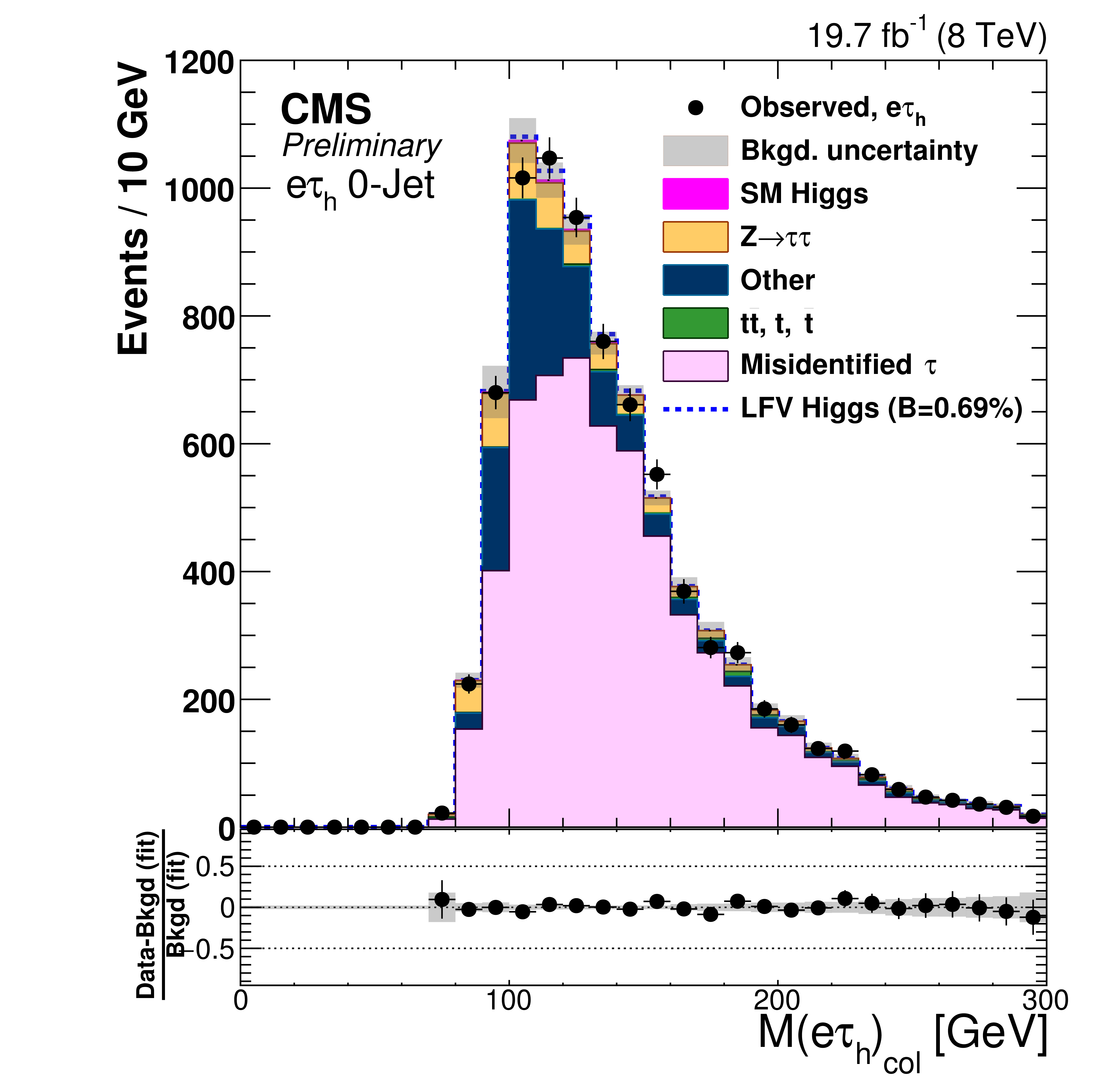
Figure 3-b:
Comparison of the observed collinear mass distributions with the background expectations after the fit. The simulated distributions for signal is shown for the branching ratio $B( {\mathrm {H}} \to {\mathrm {e}} {\tau })=0.69%$. a: $ {\mathrm {H}} \to {\mathrm {e}} {\tau }_{ {{\mu }}}$ 0-jet; b: $ {\mathrm {H}} \to {\mathrm {e}} {\tau }_{h}$ 0-jet; c: $ {\mathrm {H}} \to {\mathrm {e}} {\tau }_{ {{\mu }}}$ 1-jet; d: $ {\mathrm {H}} \to {\mathrm {e}} {\tau }_{h}$1-jet; e: $ {\mathrm {H}} \to {\mathrm {e}} {\tau }_{ {{\mu }}}$ 2-jet; f: $ {\mathrm {H}} \to {\mathrm {e}} {\tau }_{h}$ 2-jet. |
png ; pdf |
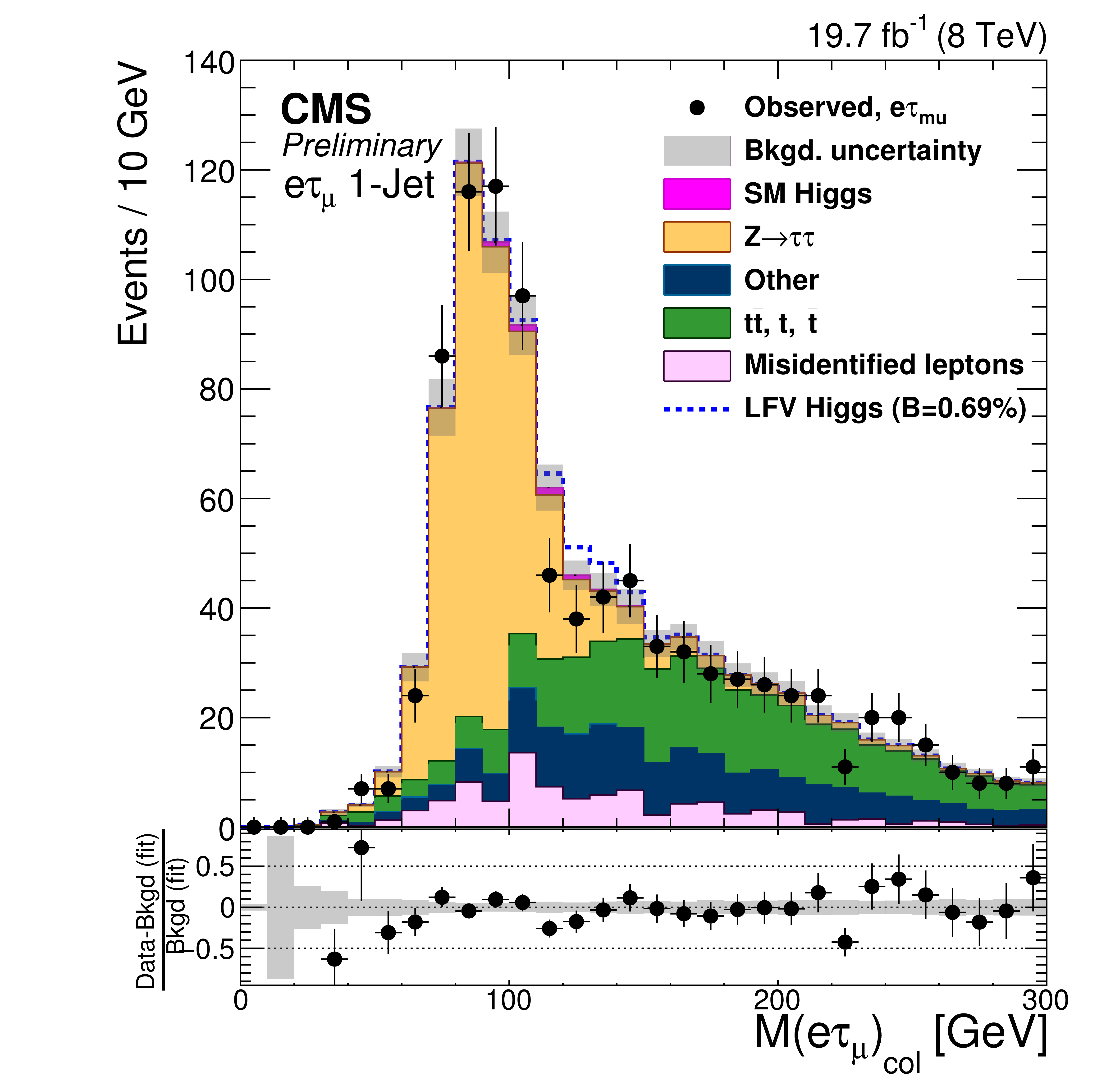
Figure 3-c:
Comparison of the observed collinear mass distributions with the background expectations after the fit. The simulated distributions for signal is shown for the branching ratio $B( {\mathrm {H}} \to {\mathrm {e}} {\tau })=0.69%$. a: $ {\mathrm {H}} \to {\mathrm {e}} {\tau }_{ {{\mu }}}$ 0-jet; b: $ {\mathrm {H}} \to {\mathrm {e}} {\tau }_{h}$ 0-jet; c: $ {\mathrm {H}} \to {\mathrm {e}} {\tau }_{ {{\mu }}}$ 1-jet; d: $ {\mathrm {H}} \to {\mathrm {e}} {\tau }_{h}$1-jet; e: $ {\mathrm {H}} \to {\mathrm {e}} {\tau }_{ {{\mu }}}$ 2-jet; f: $ {\mathrm {H}} \to {\mathrm {e}} {\tau }_{h}$ 2-jet. |
png ; pdf |
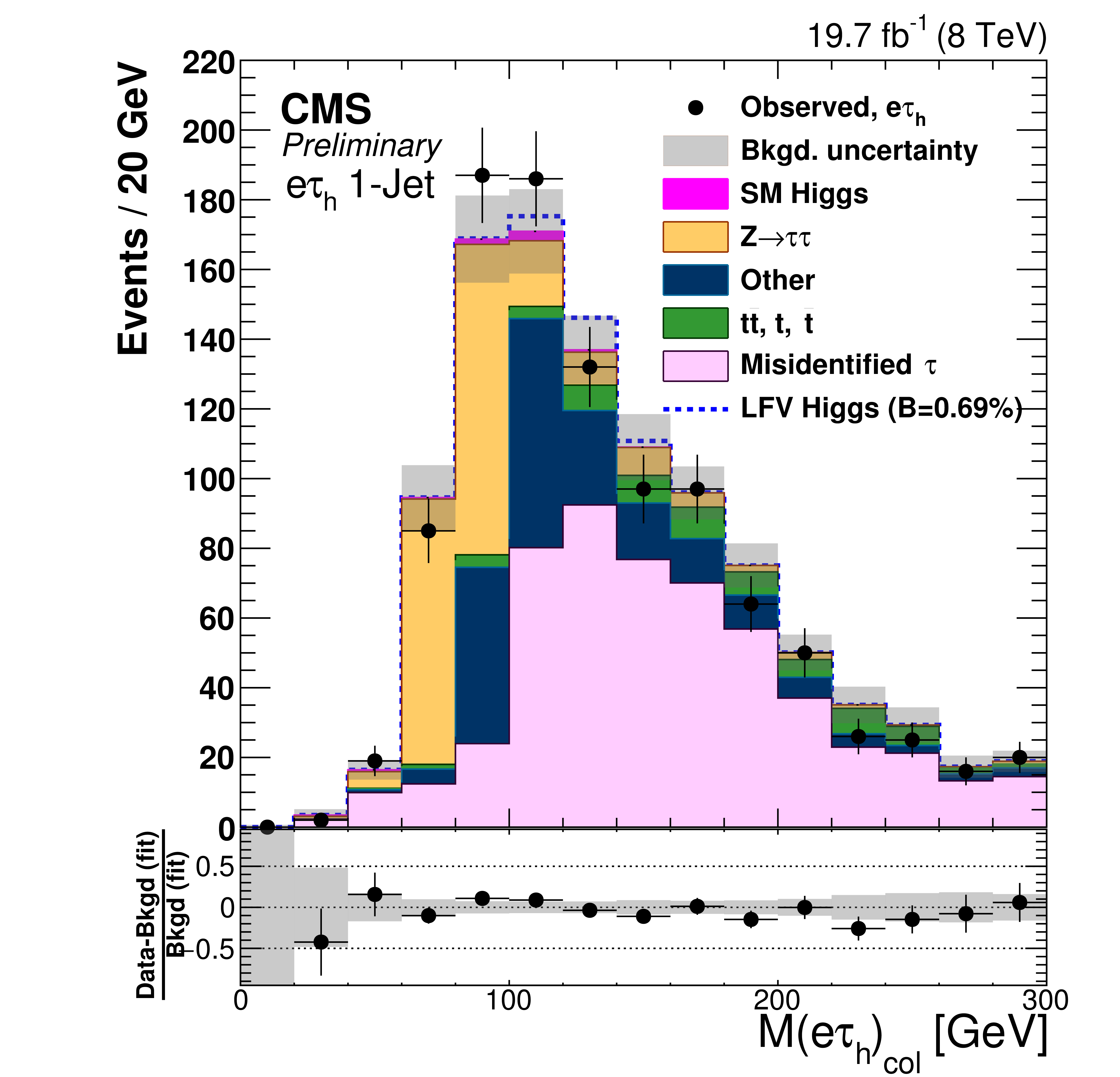
Figure 3-d:
Comparison of the observed collinear mass distributions with the background expectations after the fit. The simulated distributions for signal is shown for the branching ratio $B( {\mathrm {H}} \to {\mathrm {e}} {\tau })=0.69%$. a: $ {\mathrm {H}} \to {\mathrm {e}} {\tau }_{ {{\mu }}}$ 0-jet; b: $ {\mathrm {H}} \to {\mathrm {e}} {\tau }_{h}$ 0-jet; c: $ {\mathrm {H}} \to {\mathrm {e}} {\tau }_{ {{\mu }}}$ 1-jet; d: $ {\mathrm {H}} \to {\mathrm {e}} {\tau }_{h}$1-jet; e: $ {\mathrm {H}} \to {\mathrm {e}} {\tau }_{ {{\mu }}}$ 2-jet; f: $ {\mathrm {H}} \to {\mathrm {e}} {\tau }_{h}$ 2-jet. |
png ; pdf |
Figure 3-e:
Comparison of the observed collinear mass distributions with the background expectations after the fit. The simulated distributions for signal is shown for the branching ratio $B( {\mathrm {H}} \to {\mathrm {e}} {\tau })=0.69%$. a: $ {\mathrm {H}} \to {\mathrm {e}} {\tau }_{ {{\mu }}}$ 0-jet; b: $ {\mathrm {H}} \to {\mathrm {e}} {\tau }_{h}$ 0-jet; c: $ {\mathrm {H}} \to {\mathrm {e}} {\tau }_{ {{\mu }}}$ 1-jet; d: $ {\mathrm {H}} \to {\mathrm {e}} {\tau }_{h}$1-jet; e: $ {\mathrm {H}} \to {\mathrm {e}} {\tau }_{ {{\mu }}}$ 2-jet; f: $ {\mathrm {H}} \to {\mathrm {e}} {\tau }_{h}$ 2-jet. |

png ; pdf |
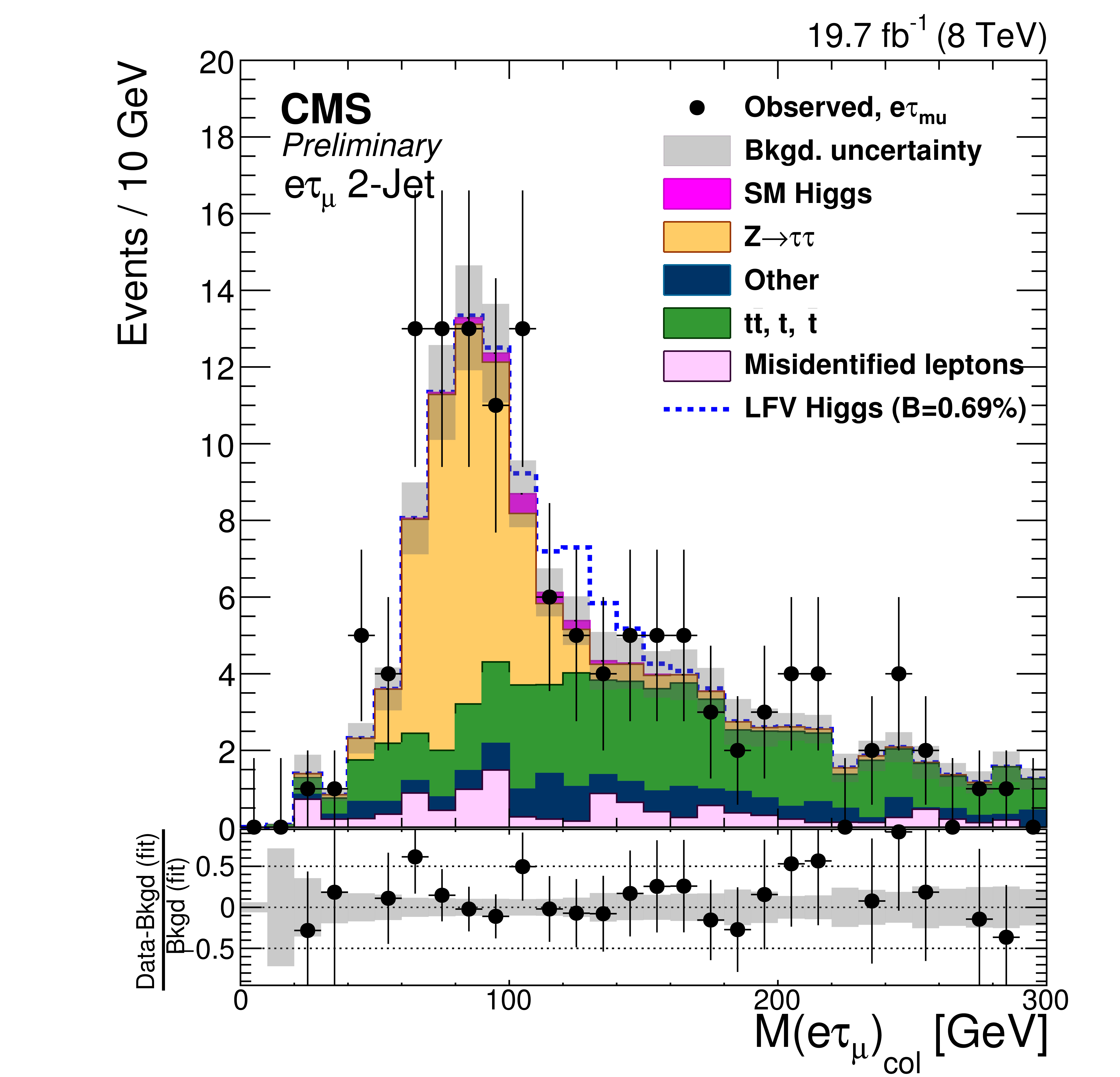
Figure 3-f:
Comparison of the observed collinear mass distributions with the background expectations after the fit. The simulated distributions for signal is shown for the branching ratio $B( {\mathrm {H}} \to {\mathrm {e}} {\tau })=0.69%$. a: $ {\mathrm {H}} \to {\mathrm {e}} {\tau }_{ {{\mu }}}$ 0-jet; b: $ {\mathrm {H}} \to {\mathrm {e}} {\tau }_{h}$ 0-jet; c: $ {\mathrm {H}} \to {\mathrm {e}} {\tau }_{ {{\mu }}}$ 1-jet; d: $ {\mathrm {H}} \to {\mathrm {e}} {\tau }_{h}$1-jet; e: $ {\mathrm {H}} \to {\mathrm {e}} {\tau }_{ {{\mu }}}$ 2-jet; f: $ {\mathrm {H}} \to {\mathrm {e}} {\tau }_{h}$ 2-jet. |
png ; pdf |
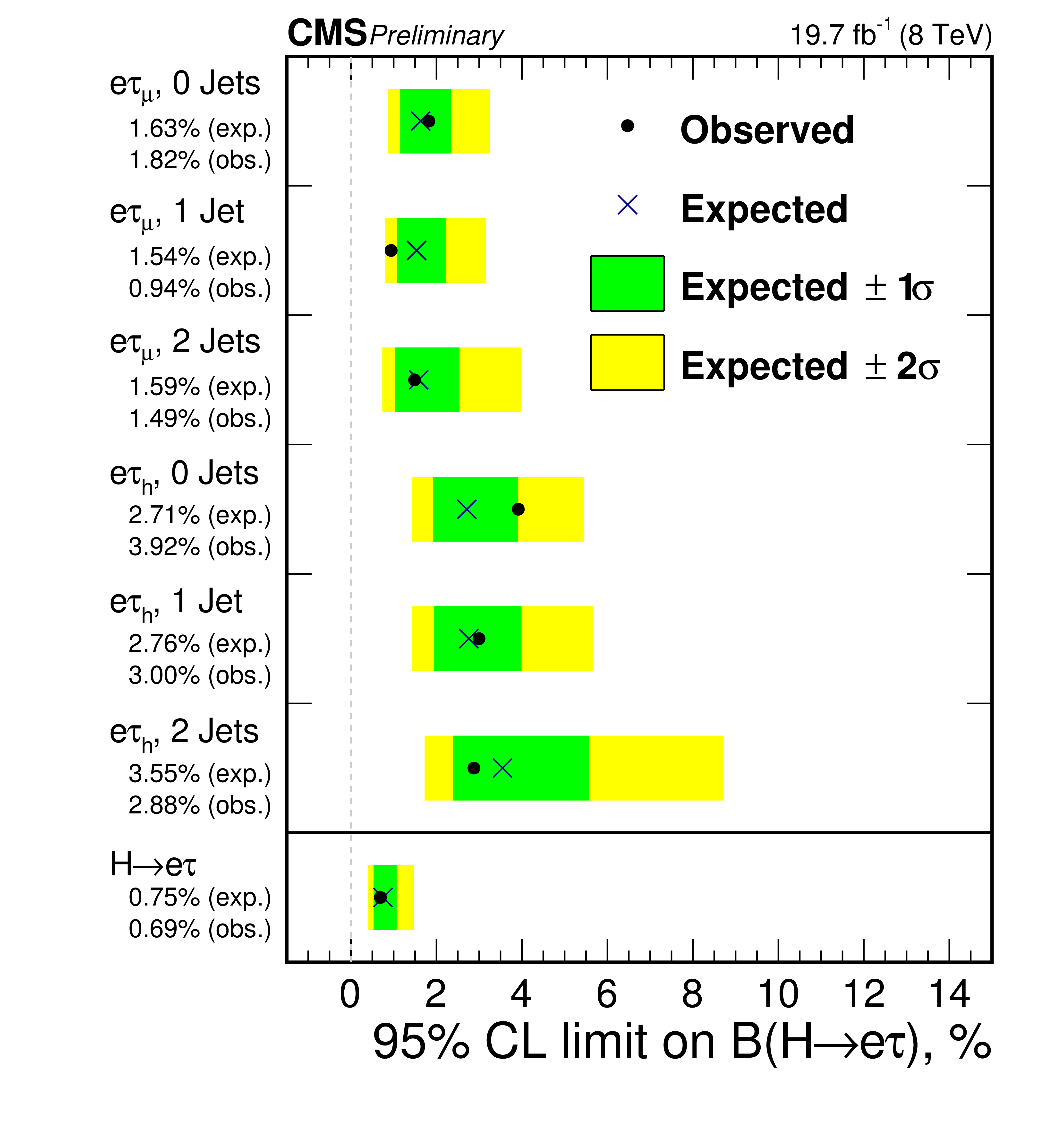
Figure 4:
Upper limits by category for the LFV $ {\mathrm {H}} \to {\mathrm {e}} {\tau }$ decays. |
png ; pdf |
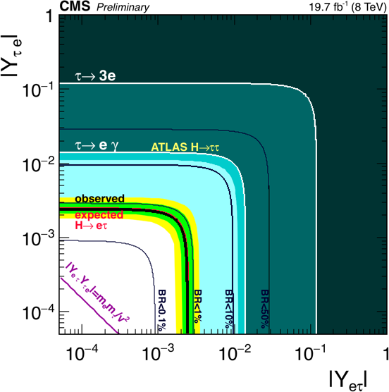
Figure 5:
Constraints on the flavour violating Yukawa couplings, $|Y_{ {\mathrm {e}} {\tau }}|,|Y_{ {\tau } {\mathrm {e}}}|$. The expected (red solid line) and observed (black solid line) limits are derived from the limit on $B( {\mathrm {H}} \to {\mathrm {e}} {\tau })$ from the present analysis. The flavour diagonal Yukawa couplings are approximated by their SM values. The green (yellow) band indicates the range that is expected to contain 68% (95%) of all observed limit excursions from the expected limit. The shaded regions are derived constraints from null searches for $ {\tau }\to 3 {\mathrm {e}}$ (dark green) and $ {\tau }\to {\mathrm {e}}\gamma $ (lighter green). The purple diagonal line is the theoretical naturalness limit $Y_{ij}Y_{ji} \leq m_im_j/v^2$. The yellow line is the limit from a theoretical reinterpretation of an ATLAS $ {\mathrm {H}} \to {\tau } {\tau }$ search. |
png ; pdf |
Figure 6-a:
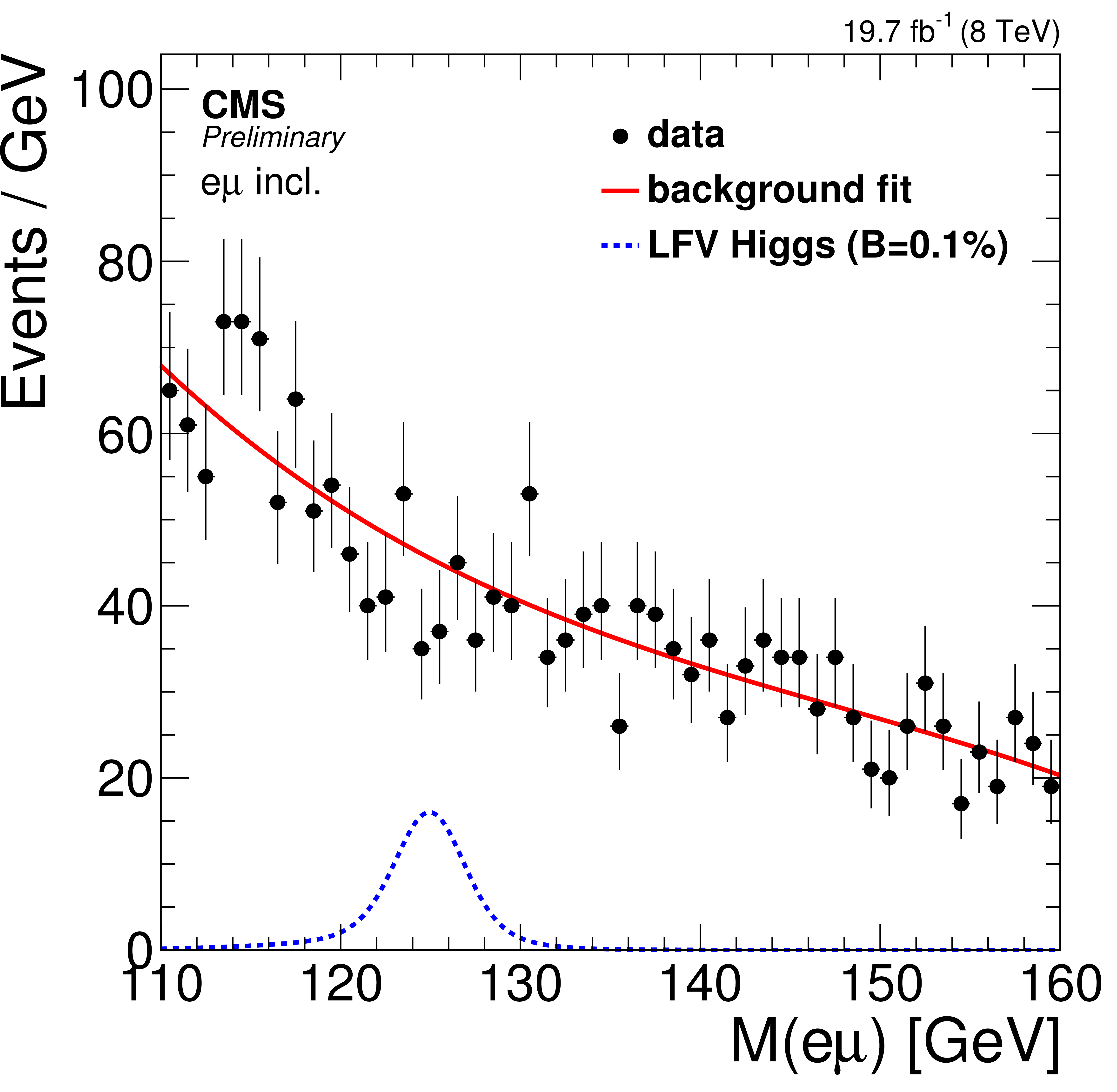
Observed $\mathrm {e}\mu $ mass spectra (points), background fit (solid line) and signal model (blue histogram) for $\mathrm{BR}( {\mathrm {H}\rightarrow \mathrm {e}\mu } ) =$ 0.1% (c). The top plots shows the results for the inclusive (a) and jet tagged (b) categories while the bottom plot shows the combination of all categories. |
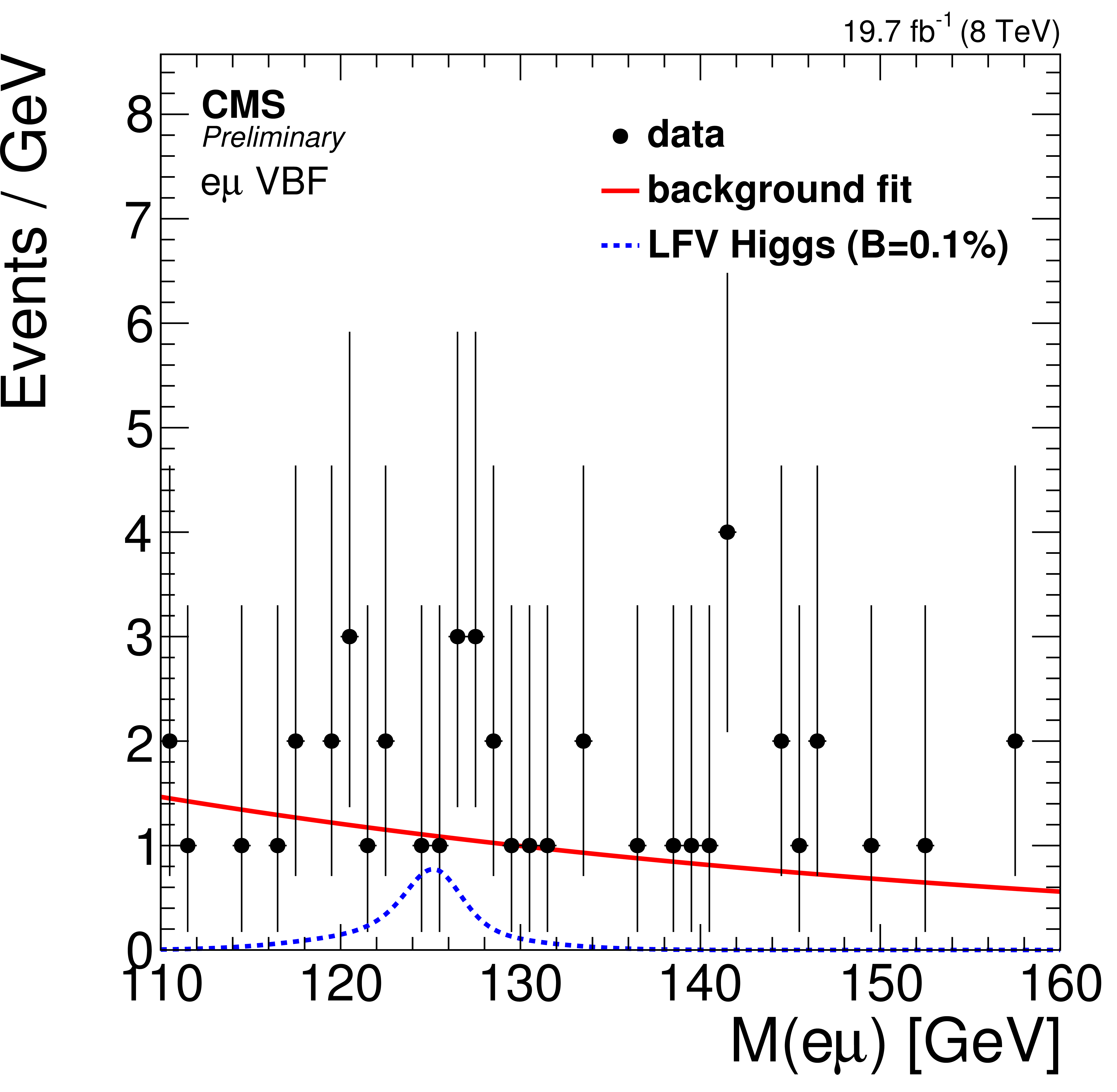
png ; pdf |
Figure 6-b:
Observed $\mathrm {e}\mu $ mass spectra (points), background fit (solid line) and signal model (blue histogram) for $\mathrm{BR}( {\mathrm {H}\rightarrow \mathrm {e}\mu } ) =$ 0.1% (c). The top plots shows the results for the inclusive (a) and jet tagged (b) categories while the bottom plot shows the combination of all categories. |

png ; pdf |
Figure 6-c:
Observed $\mathrm {e}\mu $ mass spectra (points), background fit (solid line) and signal model (blue histogram) for $\mathrm{BR}( {\mathrm {H}\rightarrow \mathrm {e}\mu } ) =$ 0.1% (c). The top plots shows the results for the inclusive (a) and jet tagged (b) categories while the bottom plot shows the combination of all categories. |

png ; pdf |
Figure 7:
Upper limit on $\mathrm {BR}( {\mathrm {H}\rightarrow \mathrm {e}\mu } )$ at $ {M_{ {\mathrm {H}} }}=$ 125 GeV for inclusive categories grouped by number of jets, jet tagged and all categories combined. |
png ; pdf |
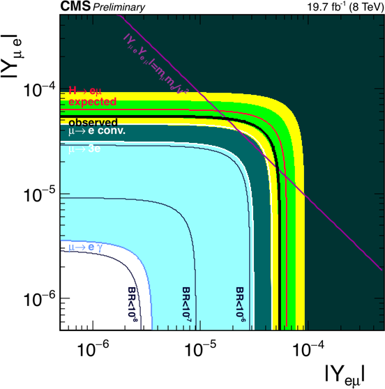
Figure 8:
Constraints on the flavour violating Yukawa couplings, $|Y_{ {\mathrm {e}} {{\mu }}}|,|Y_{ {{\mu }} {\mathrm {e}}}|$. The expected (red solid line) and observed (black solid line) limits are derived from the limit on $B( {\mathrm {H}} \to {\mathrm {e}} {{\mu }})$ from the present analysis. The flavour diagonal Yukawa couplings are approximated by their SM values. The green (yellow) band indicates the range that is expected to contain 68% (95%) of all observed limit excursions from the expected limit. The shaded regions are derived constraints from null searches for $ {{\mu }}\to {\mathrm {e}}$ conversion (dark green), $ {{\mu }}\to 3 {\mathrm {e}}$ (light green), and $ {\tau }\to {\mathrm {e}}\gamma $ (cyan). The purple diagonal line is the theoretical naturalness limit $Y_{ij}Y_{ji} \leq m_im_j/v^2$. |
| Tables | |
png ; pdf |
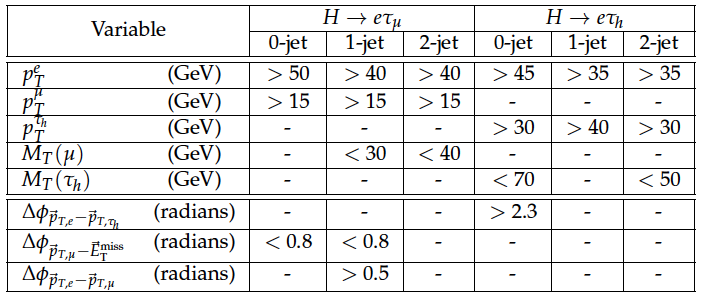
Table 1:
Selection criteria requirements for the kinematic variables after the loose selection. |
png ; pdf |
Table 2:
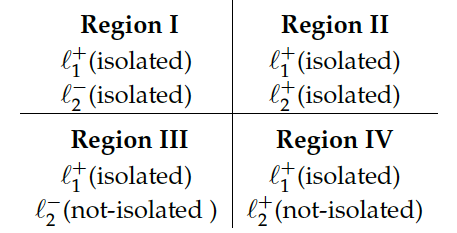
Schematic to illustrate the application of the method used to estimate the misidentified lepton ($\ell $) background. Samples are defined by the charge of the two leptons and by the isolation requirements on each. Charged conjugates are assumed. |
png ; pdf |
Table 3:
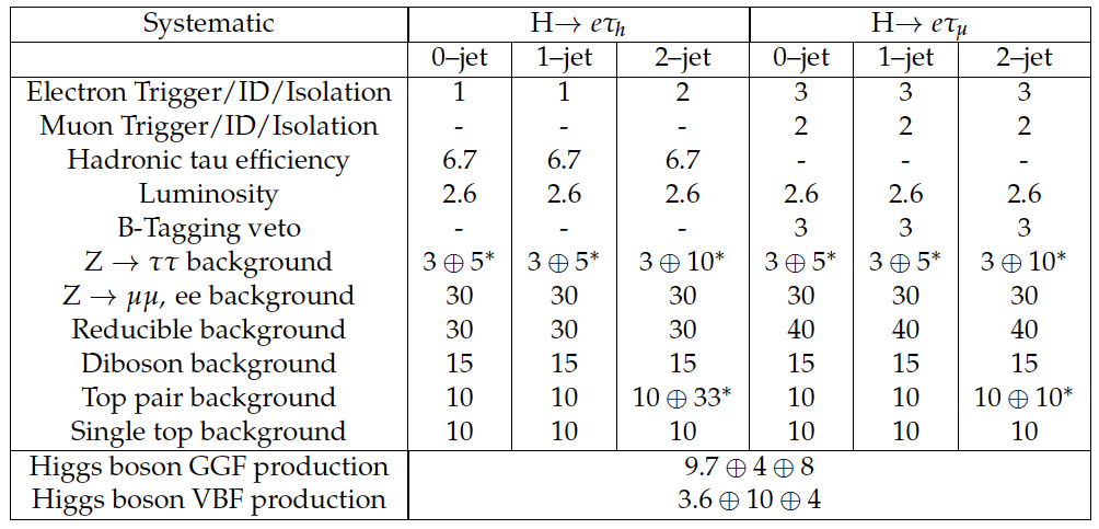
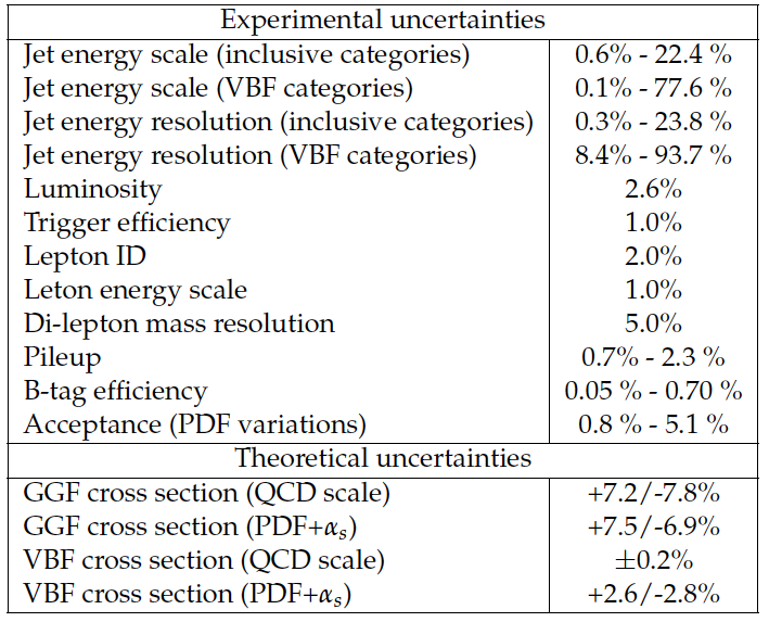
Systematic uncertainties on the expected yield in % for the $ {\mathrm {e}}\tau _{h}$ and $ {\mathrm {e}}\tau _{\mu }$ channels. All uncertainties are treated as correlated between the categories, except if there are two values quoted. In this case the number denoted with * is treated as uncorrelated between categories. |
png ; pdf |
Table 4:
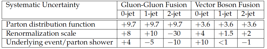
Theoretical uncertainties in % for Higgs boson production cross section. Anticorrelations arise due to migration of events between the categories and are expressed as negative numbers. |
png ; pdf |
Table 5:
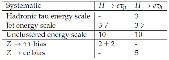
Systematic uncertainties in the shape of the signal and background templates, expressed in %. |

png ; pdf |
Table 6:
Selection criteria for each of the categories used in this analysis. The EB-MB (ME) categories include only events with the electron in the calorimeter barrel $|\eta _{e}| < 1.479$ and the muon in the muon detector barrel (endcap) $|\eta _{\mu }| < 0.8$ ($|\eta _{\mu }| > 0.8$). In the EE-(MB or ME) categories the electron is required to be in the calorimeter endcap ($|\eta _{e}| < 1.566$), while no selection is applied to the muon pseudorapidity. |

png ; pdf |
Table 7:
Selected functions and orders for background model in each category. |
png ; pdf |
Table 8:
Systematic uncertainties on the expected yield for the $ {\mathrm {H}} \to {\mathrm {e}} {{\mu }}$. All uncertainties have been considered as correlated between categories. |
png ; pdf |
Table 9:
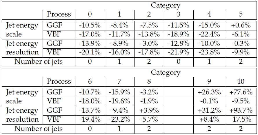
Relative change of signal yields when varying the jet energy scale or the jet energy resolution within uncertainties. For reference, the requirement on the number of reconstructed jets is shown in the bottom row. |
png ; pdf |
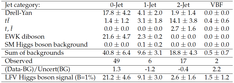
Table 10:
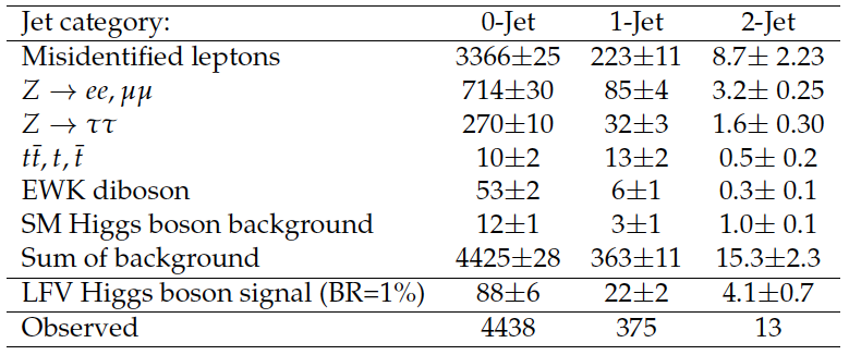
Event yield after the fit in the mass window 100 $ < M_{collinear} < $ 150 GeV for the $ {\mathrm {H}} \rightarrow {\mathrm {e}}\tau _{h}$ channel. The contributions are normalized to an integrated luminosity of 19.7 fb$^{-1}$. The LFV Higgs boson signal is the MC expectation for B($ {\mathrm {H}} \rightarrow {\mathrm {e}}\tau )=1%$. |
png ; pdf |
Table 11:
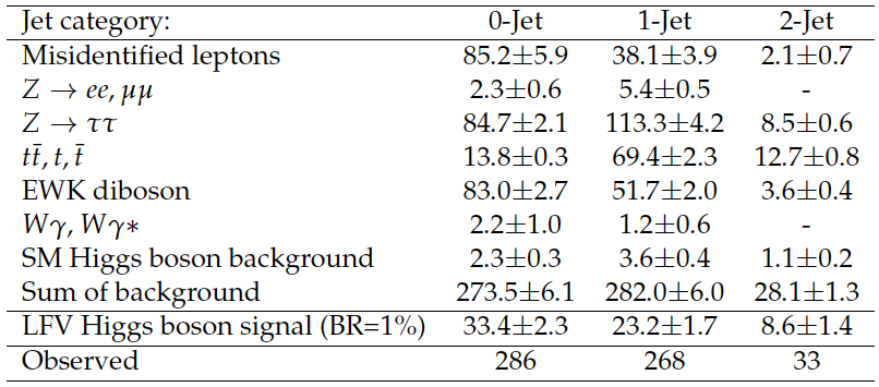
Event yield after the fit in the mass window 100 $ < M_{collinear} < $ 150 GeV for the $ {\mathrm {H}} \rightarrow {\mathrm {e}}\tau _{\mu }$ channel. The contributions are normalized to an integrated luminosity of 19.7fb$^{-1}$. The LFV Higgs boson signal is the MC expectation for B($ {\mathrm {H}} \rightarrow {\mathrm {e}}\tau )=1%$. "-" indicates that 0 MC events for the particular background are selected. |
png ; pdf |
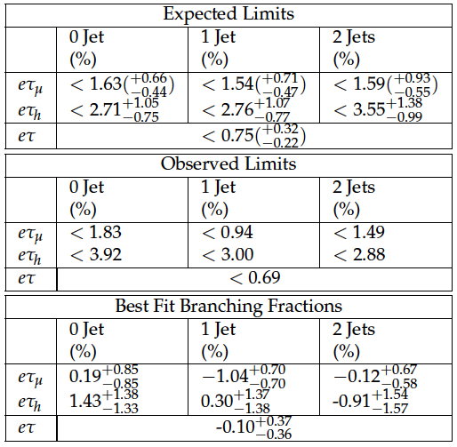
Table 12:
The expected upper limits, observed limits and best fit values for the branching fractions $B( {\mathrm {H}} \to {\mathrm {e}}\tau )$ for different jet categories and analysis channels. The one standard-deviation probability intervals around the expected limits are shown in parentheses. |
png ; pdf |
Table 13:
Event yields in the mass window 124 $ < m_{e\mu } < $ 126 GeV for the $ {\mathrm {H}\rightarrow \mathrm {e}\mu } $ channel. The expected contributions are normalized to an integrated luminosity of 19.7fb$^{-1}$. The LFV Higgs boson signal is the MC expectation for B($ {\mathrm {H}\rightarrow \mathrm {e}\mu } =0.1%$). |
|
|
Compact Muon Solenoid LHC, CERN |
|

|

|

|

|

|