

Compact Muon Solenoid
LHC, CERN
| CMS-PAS-FSQ-13-008 | ||
| Evidence for exclusive gamma-gamma to $\mathrm{W^+ W^-}$ production and constraints on Anomalous Quartic Gauge Couplings at $ \sqrt{s} =$ 8 TeV | ||
| CMS Collaboration | ||
| June 2015 | ||
| Abstract: A search for exclusive or quasi-exclusive $\gamma\gamma \rightarrow \mathrm{ W^{+}W^{-} }$ production, $ \mathrm{pp \rightarrow p^{(*)} W^{+}W^{-} p^{(*)} \to p^{(*)} \mu^{\pm} e^{\mp} p^{(*)} } $, at $\sqrt{s} =$ 8 TeV is reported using data corresponding to an integrated luminosity of 19.7 fb$^{-1}$. Events are selected by requiring the presence of an electron-muon pair with large transverse momentum $p_{\mathrm{T}}(\mu^{\pm} \mathrm{e}^{\mp})> $ 30 GeV and no associated charged particles detected from the same vertex. In the signal region 13 events are observed over an expected background of 3.5 $\pm$ 0.5 events, corresponding to an excess of 3.6$\sigma$ over the background-only hypothesis. The observed yields and kinematic distributions are compatible with the Standard Model prediction for exclusive and quasi-exclusive $\gamma\gamma \rightarrow \mathrm{ W^{+}W^{-} } $ production. The dilepton transverse momentum spectrum is studied for deviations from the Standard Model, and the resulting upper limits are compared to predictions assuming anomalous quartic gauge couplings. | ||
|
Links:
CDS record (PDF) ;
Public twiki page ;
CADI line (restricted) ; Figures are also available from the CDS record. These preliminary results are superseded in this paper, JHEP 08 (2016) 119. |
||
| Figures | |
png ; pdf |
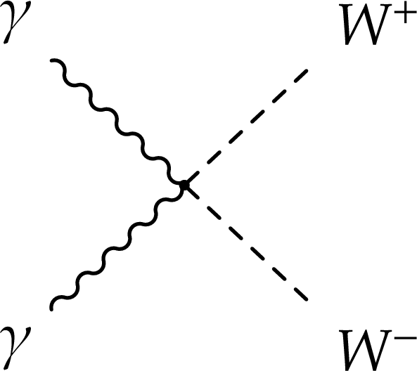
Figure 1-a:
Quartic and t-channel diagrams contributing to the $\mathrm{ \gamma \gamma \to W^{+}W^{-}}$ process at leading order in the SM. |
png ; pdf |
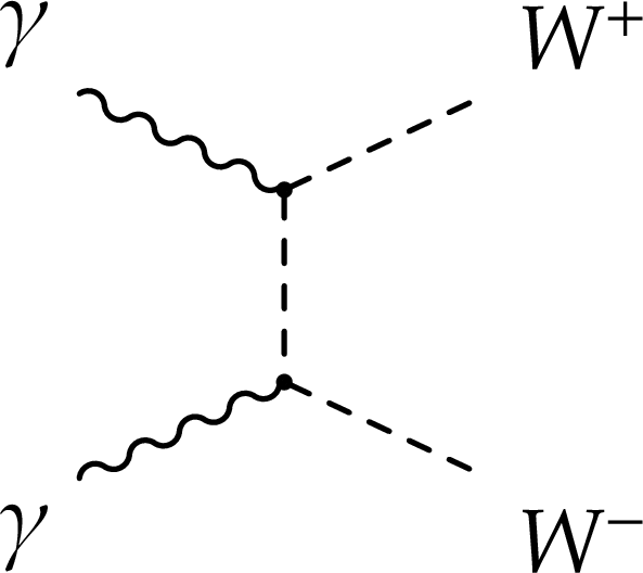
Figure 1-b:
Quartic and t-channel diagrams contributing to the $\mathrm{ \gamma \gamma \to W^{+}W^{-}}$ process at leading order in the SM. |
png ; pdf |
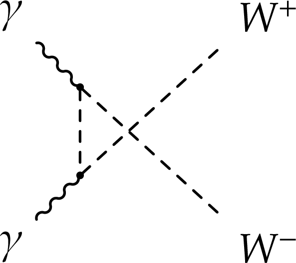
Figure 1-c:
Quartic and t-channel diagrams contributing to the $\mathrm{ \gamma \gamma \to W^{+}W^{-}}$ process at leading order in the SM. |
png ; pdf |
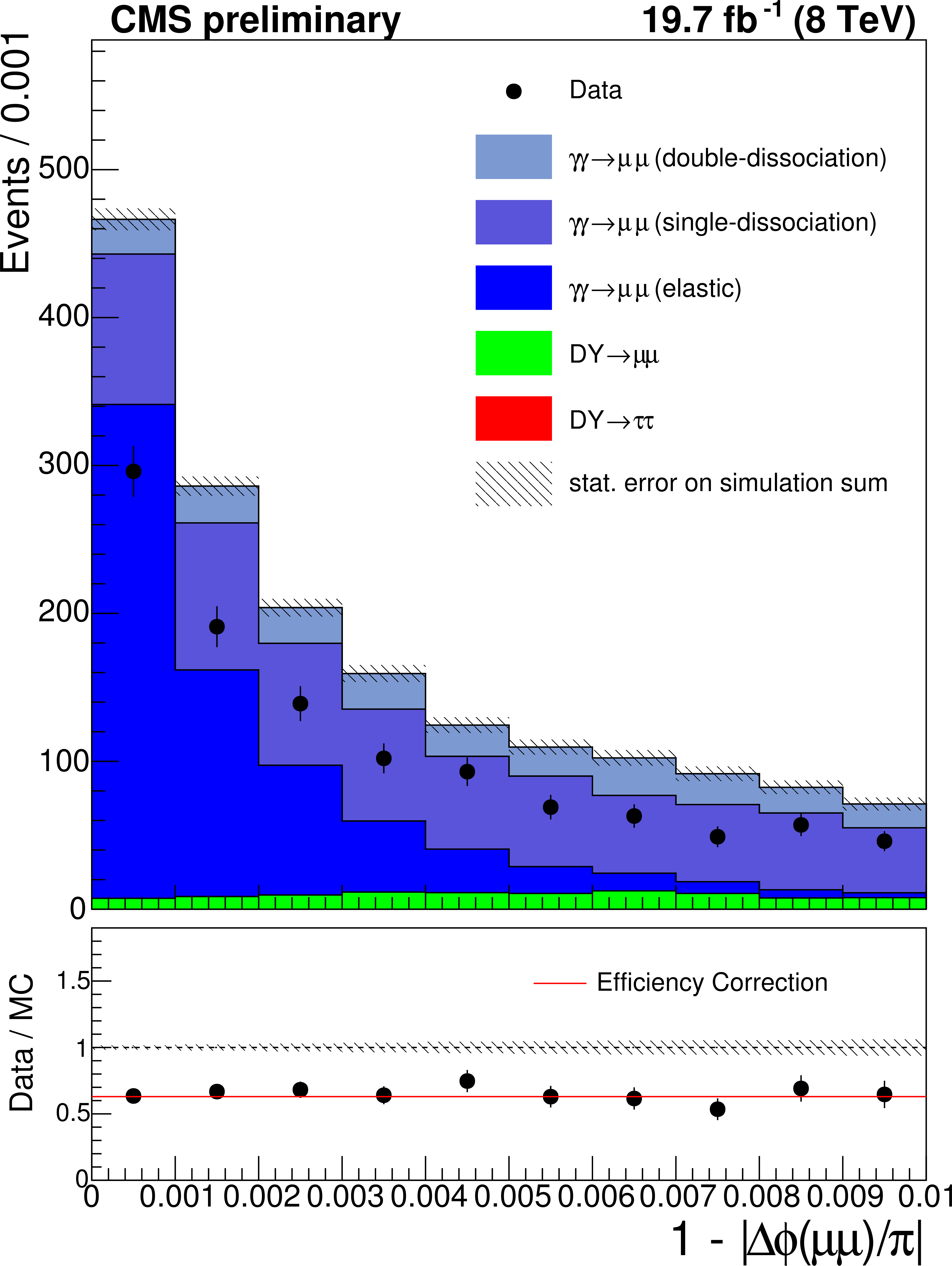
Figure 2-a:
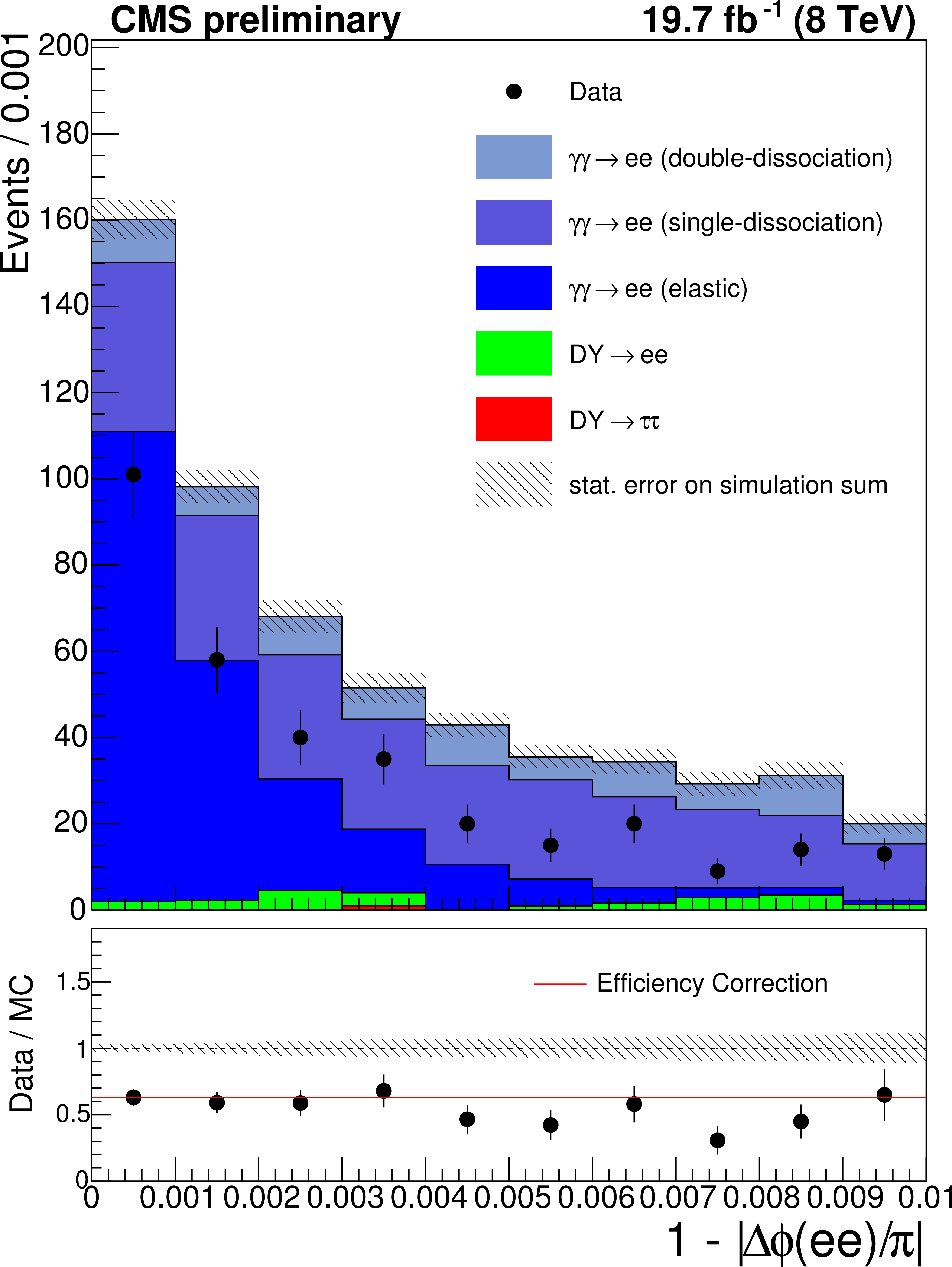
The acoplanarity for the $\mu ^{+} \mu ^{-}$ (a) and $e^{+}e^{-}$ (b) final states in the elastic $\gamma \gamma \rightarrow \ell ^{+}\ell ^{-}$ control region with an invariant mass incompatible with $Z \rightarrow \ell ^{+}\ell ^{-}$ decays ($m(\ell ^{+}\ell ^{-}) < 70$ GeV or $m(\ell ^{+}\ell ^{-}) > 106$ GeV). The red line shows the calculated correction to the 0 extra tracks efficiency. |
png ; pdf |
Figure 2-b:
The acoplanarity for the $\mu ^{+} \mu ^{-}$ (a) and $e^{+}e^{-}$ (b) final states in the elastic $\gamma \gamma \rightarrow \ell ^{+}\ell ^{-}$ control region with an invariant mass incompatible with $Z \rightarrow \ell ^{+}\ell ^{-}$ decays ($m(\ell ^{+}\ell ^{-}) < 70$ GeV or $m(\ell ^{+}\ell ^{-}) > 106$ GeV). The red line shows the calculated correction to the 0 extra tracks efficiency. |
png ; pdf |
Figure 3-a:
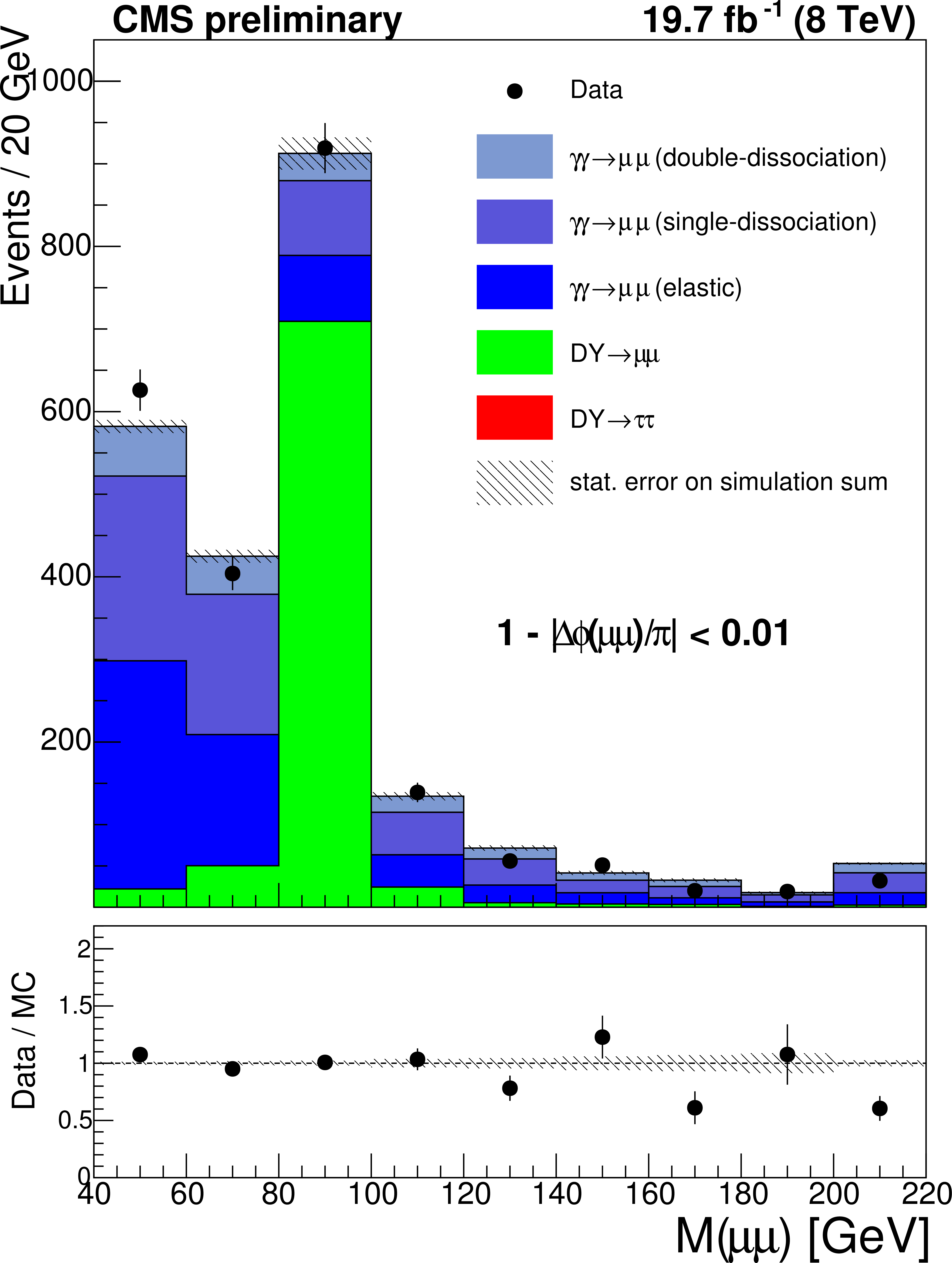
The dilepton invariant mass for the $\mu ^{+} \mu ^{-}$ (a) and $e^{+}e^{-}$ (b) final states in the elastic $\gamma \gamma \rightarrow \ell ^{+}\ell ^{-}$ control region. The exclusive simulation is scaled to the number of events in data for $m(\ell ^{+}\ell ^{-}) < 70$ GeV or $m(\ell ^{+}\ell ^{-}) > 106$ GeV. The Drell-Yan simulation is scaled to the number of events in data for $m(\ell ^{+}\ell ^{-}) > 70$ GeV or $m(\ell ^{+}\ell ^{-}) < 106$ GeV The last bin in both plots is an overflow bin and includes all events with invariant mass greater than 220 GeV. |
png ; pdf |
Figure 3-b:
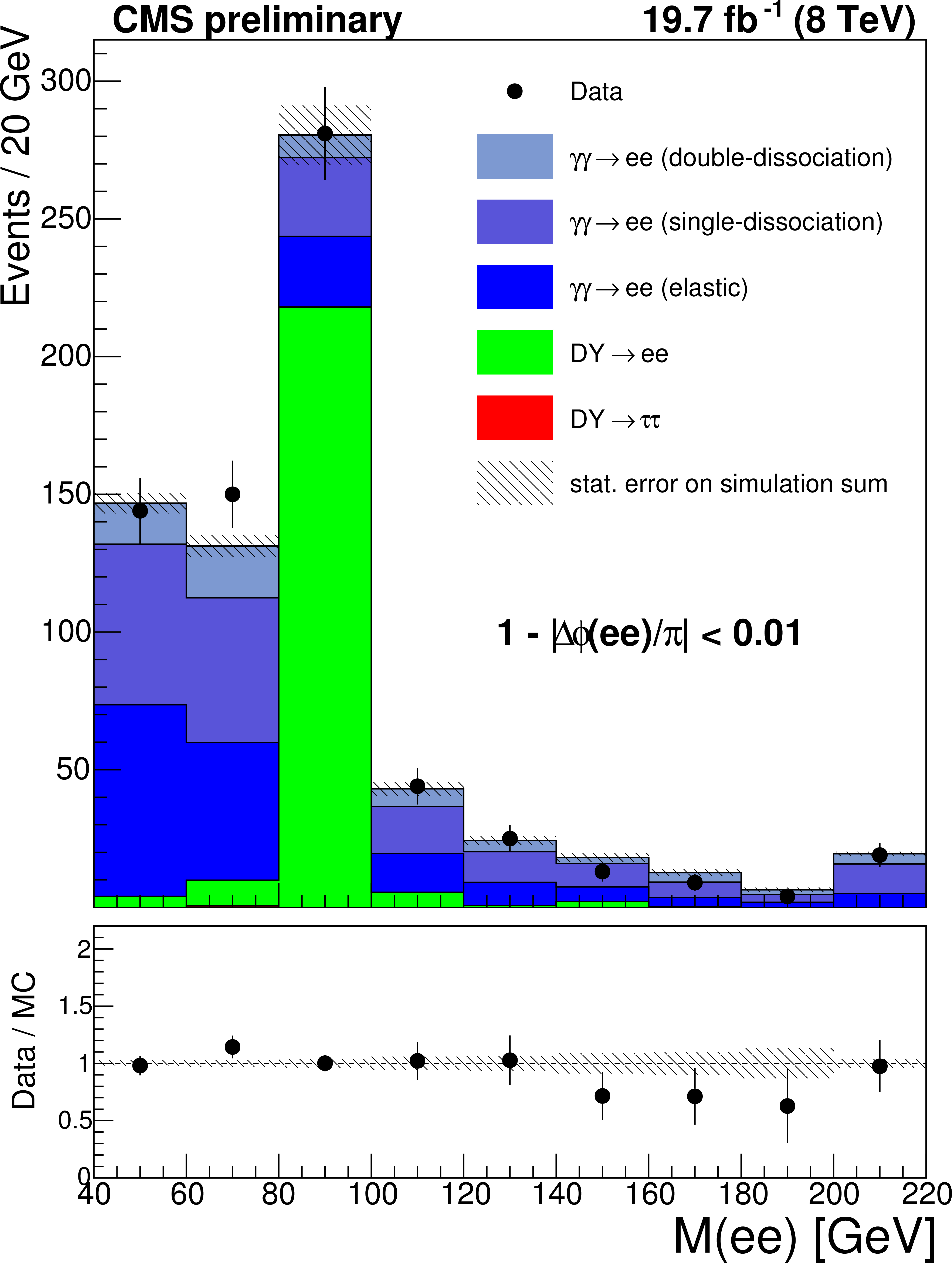
The dilepton invariant mass for the $\mu ^{+} \mu ^{-}$ (a) and $e^{+}e^{-}$ (b) final states in the elastic $\gamma \gamma \rightarrow \ell ^{+}\ell ^{-}$ control region. The exclusive simulation is scaled to the number of events in data for $m(\ell ^{+}\ell ^{-}) < 70$ GeV or $m(\ell ^{+}\ell ^{-}) > 106$ GeV. The Drell-Yan simulation is scaled to the number of events in data for $m(\ell ^{+}\ell ^{-}) > 70$ GeV or $m(\ell ^{+}\ell ^{-}) < 106$ GeV The last bin in both plots is an overflow bin and includes all events with invariant mass greater than 220 GeV. |
png ; pdf |
Figure 4-a:
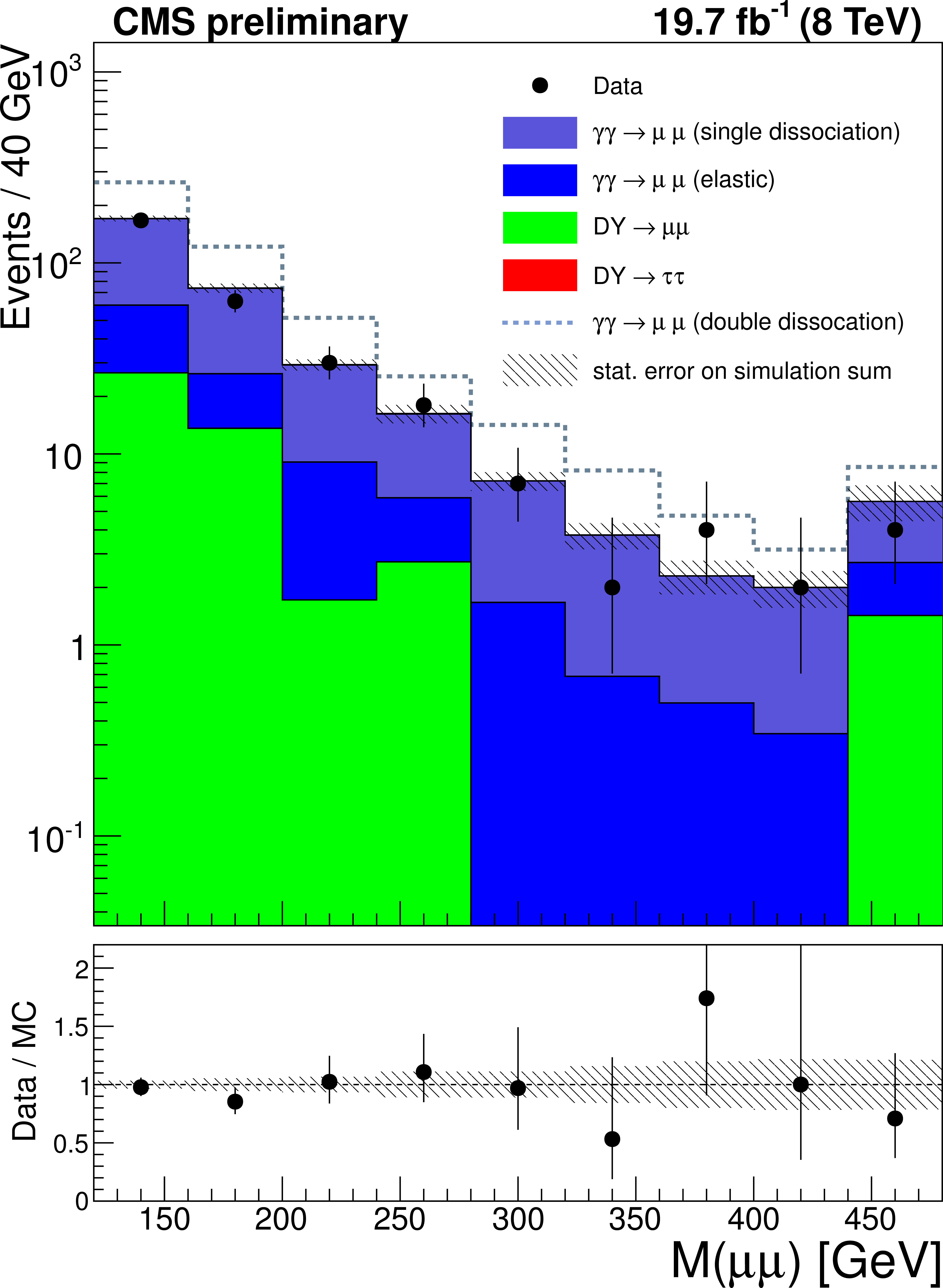
The dilepton invariant mass for the $\mu ^{+}\mu ^{-}$ (a) and $e^{+}e^{-}$ (b) final states in the $\gamma \gamma \rightarrow \ell ^{+}\ell ^{-}$ proton dissociation control region with 0 additional tracks associated to the dilepton vertex. The efficiency correction has been applied to the exclusive samples. The double-dissociation contribution in the simulation is much too large because of rescattering effects. Therefore, the double-dissociation contribution is not included in the ratio plot and is shown as the blue dotted line on top of the sum of the simulation. The region $m(\ell ^{+}\ell ^{-})>160$ GeV is used to obtain the proton dissociation contribution. The last bin is an overflow bin and includes all events above 480 GeV. |
png ; pdf |
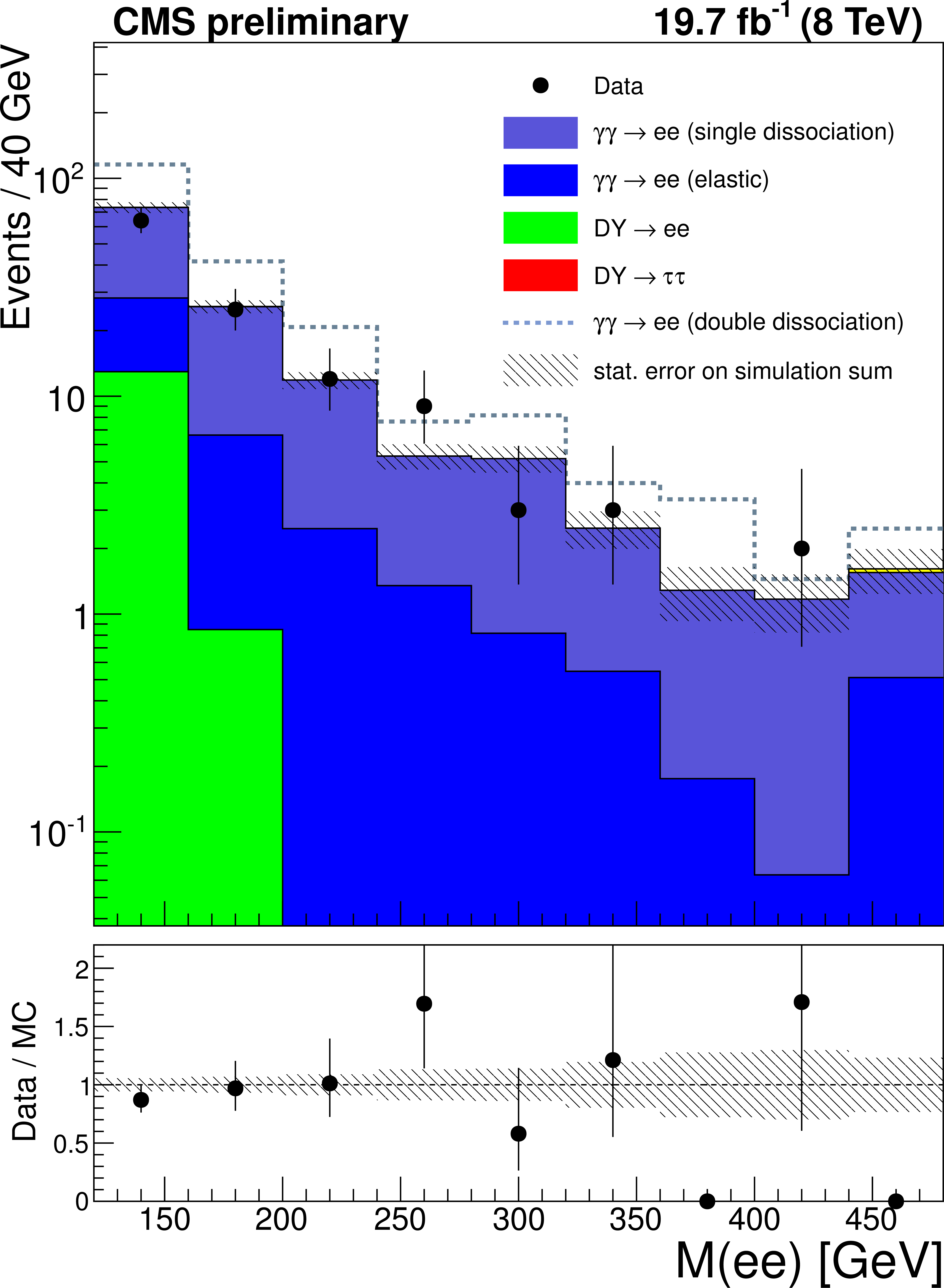
Figure 4-b:
The dilepton invariant mass for the $\mu ^{+}\mu ^{-}$ (a) and $e^{+}e^{-}$ (b) final states in the $\gamma \gamma \rightarrow \ell ^{+}\ell ^{-}$ proton dissociation control region with 0 additional tracks associated to the dilepton vertex. The efficiency correction has been applied to the exclusive samples. The double-dissociation contribution in the simulation is much too large because of rescattering effects. Therefore, the double-dissociation contribution is not included in the ratio plot and is shown as the blue dotted line on top of the sum of the simulation. The region $m(\ell ^{+}\ell ^{-})>160$ GeV is used to obtain the proton dissociation contribution. The last bin is an overflow bin and includes all events above 480 GeV. |
png ; pdf |
Figure 5-a:
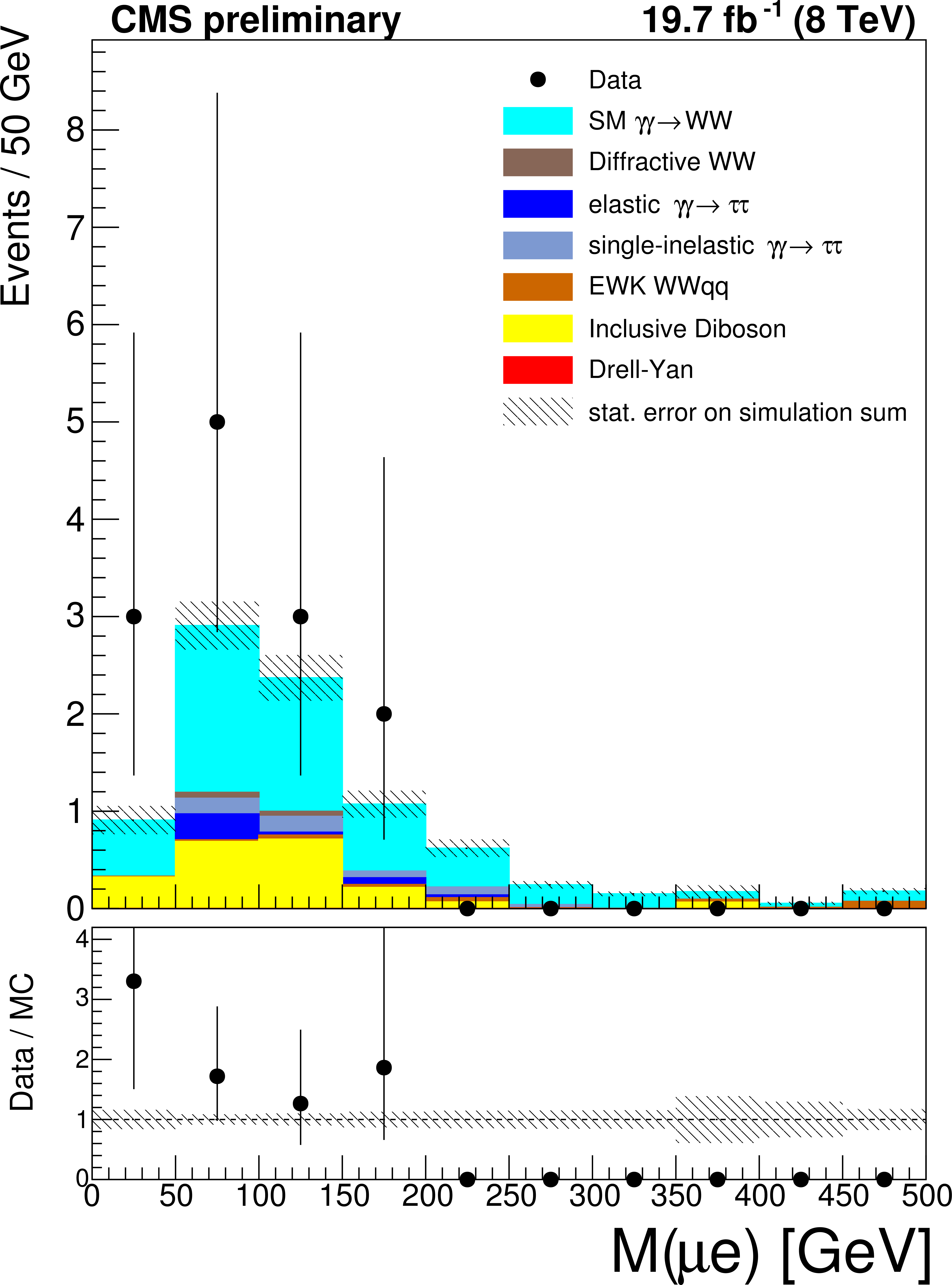
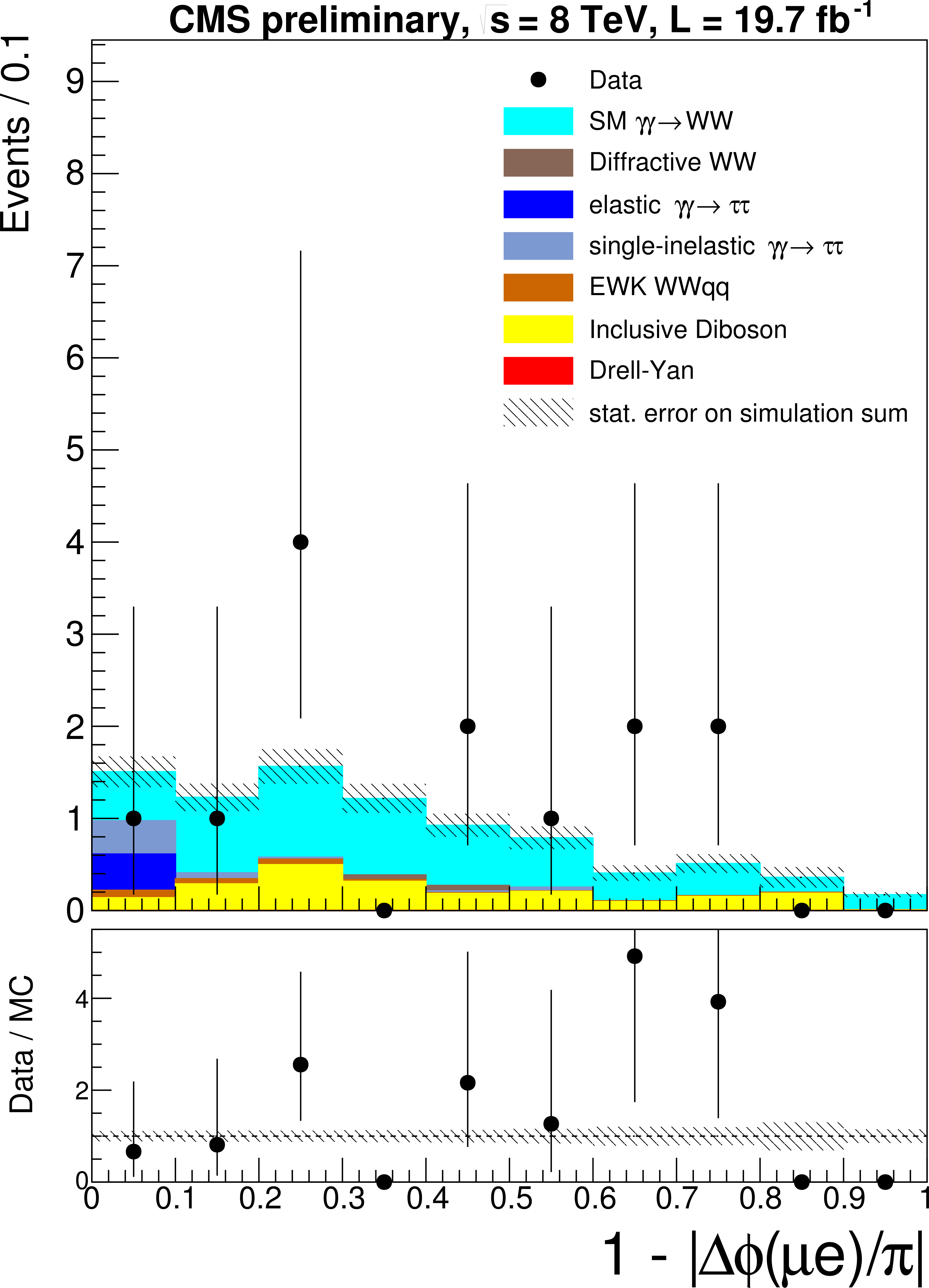
The $\mu ^{\pm }e^{\mp }$ invariant mass (a) and acoplanarity (b) are shown for data and the expected backgrounds for $p_{T}(\mu ^{\pm }e^{\mp }) > 30$ GeV and 1-6 extra tracks (inclusive $W^{+}W^{-}$ control region). The last bin in the invariant mass plot is an overflow bin and includes all events above 500 GeV. |
png ; pdf |
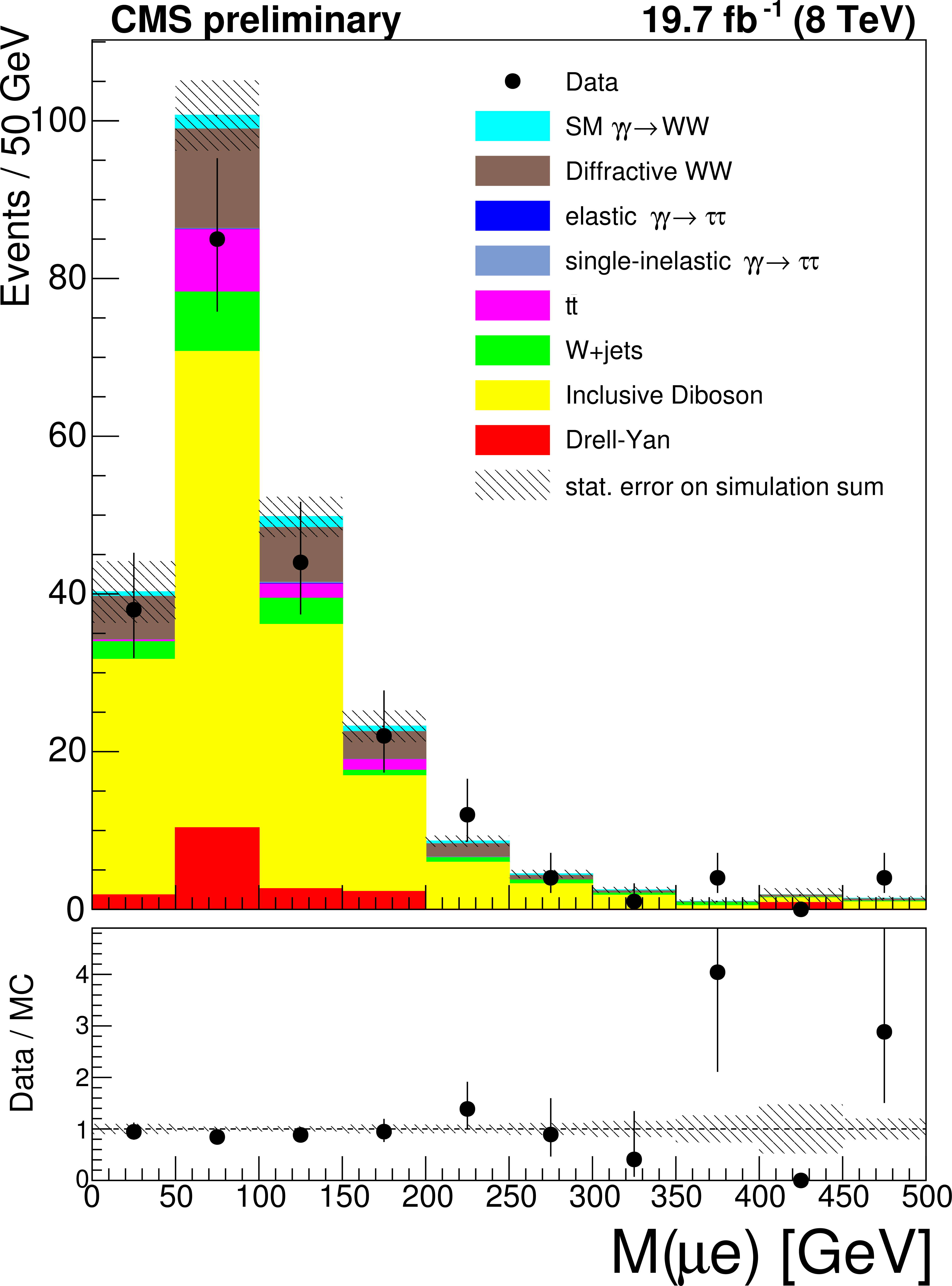
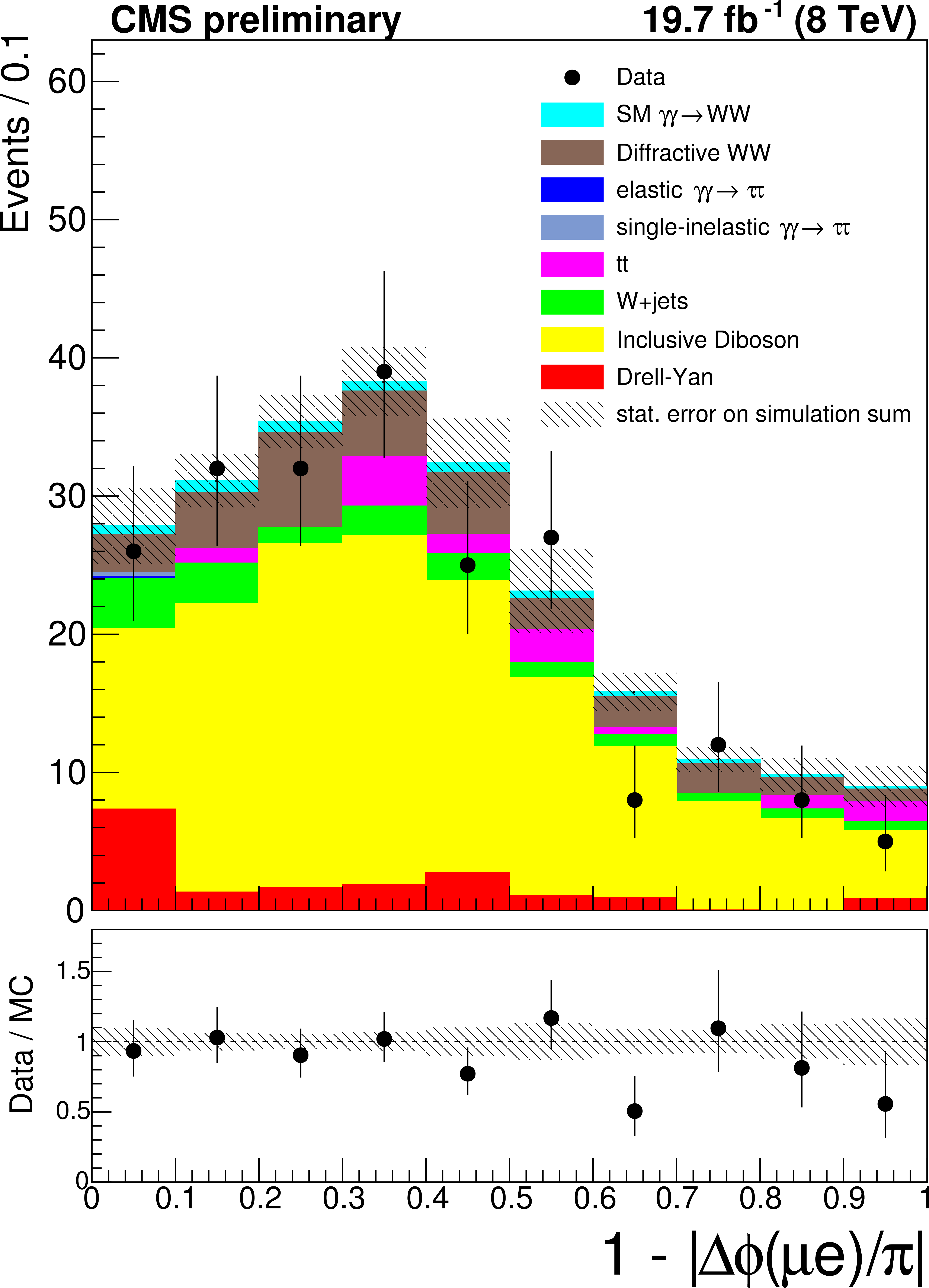
Figure 5-b:
The $\mu ^{\pm }e^{\mp }$ invariant mass (a) and acoplanarity (b) are shown for data and the expected backgrounds for $p_{T}(\mu ^{\pm }e^{\mp }) > 30$ GeV and 1-6 extra tracks (inclusive $W^{+}W^{-}$ control region). The last bin in the invariant mass plot is an overflow bin and includes all events above 500 GeV. |
png ; pdf |
Figure 6-a:
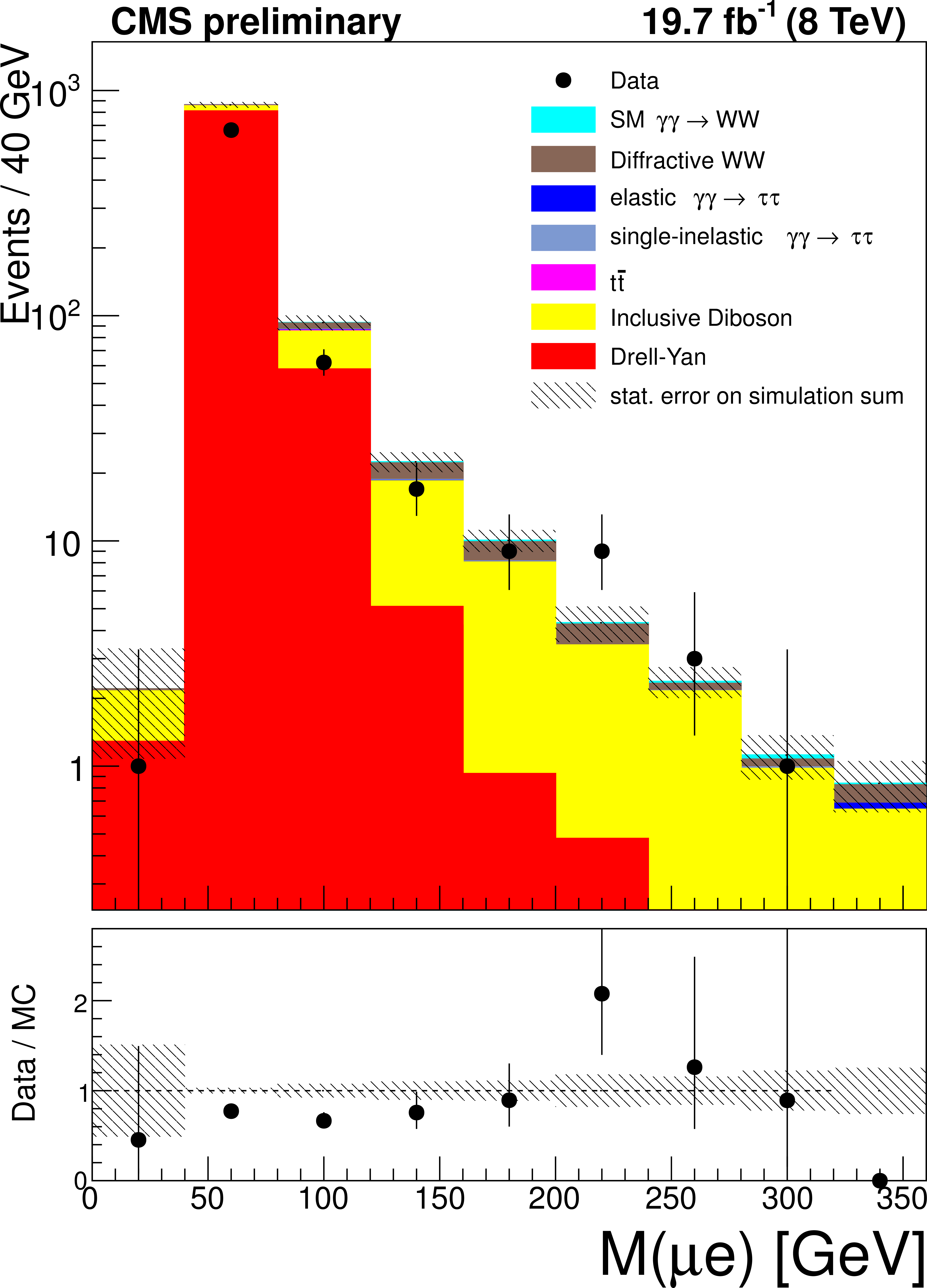
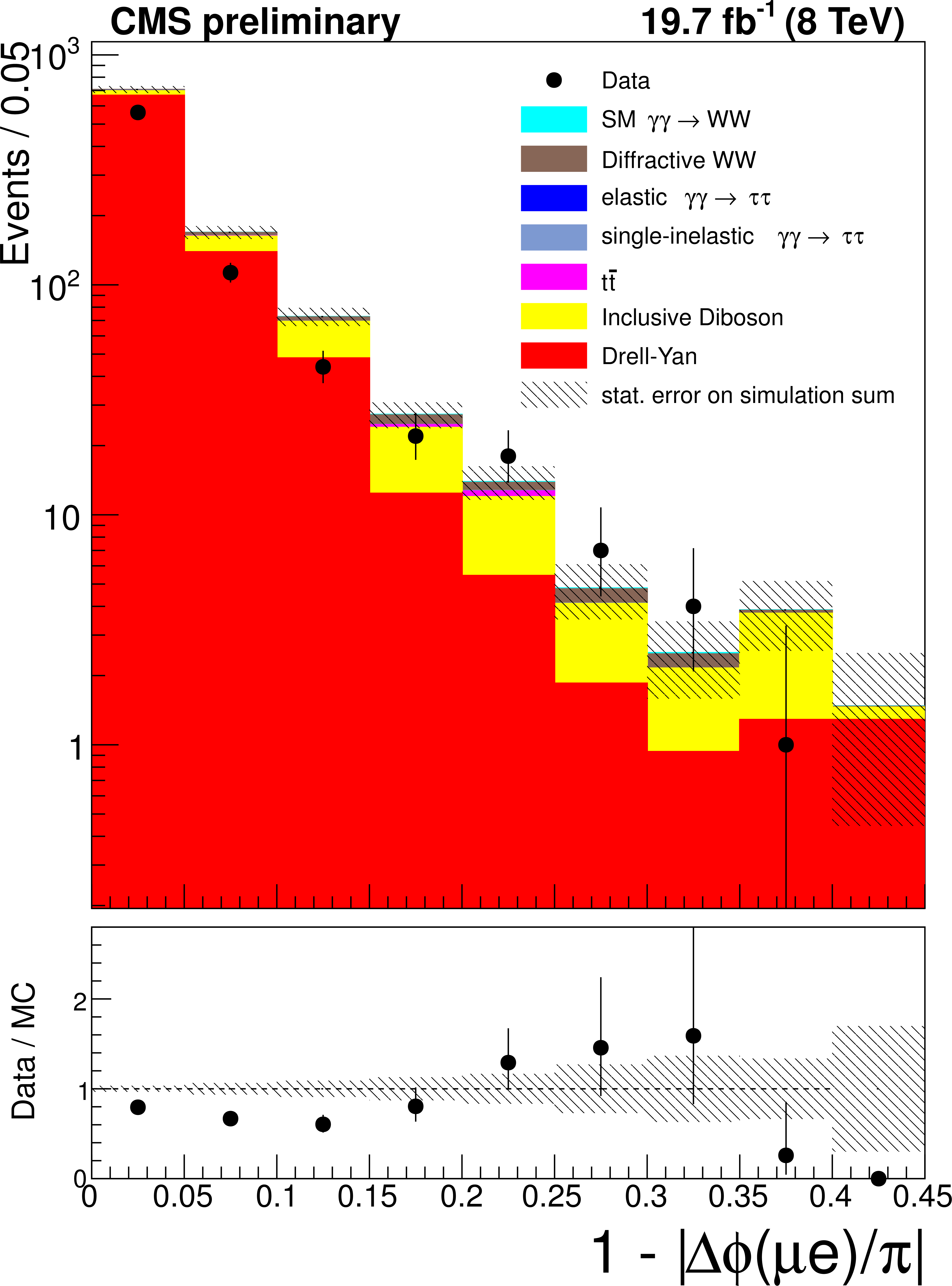
The $\mu ^{\pm }e^{\mp }$ invariant mass (a) and acoplanarity (b) are shown for data and the expected backgrounds for $p_{T}(\mu ^{\pm }e^{\mp }) < 30$ GeV and 1-6 extra tracks (Drell-Yan $\tau ^{+}\tau ^{-}$ control region). The last bin in the acoplanarity distribution is an overflow bin and includes all events above acoplanarity 0.4. |
png ; pdf |
Figure 6-b:
The $\mu ^{\pm }e^{\mp }$ invariant mass (a) and acoplanarity (b) are shown for data and the expected backgrounds for $p_{T}(\mu ^{\pm }e^{\mp }) < 30$ GeV and 1-6 extra tracks (Drell-Yan $\tau ^{+}\tau ^{-}$ control region). The last bin in the acoplanarity distribution is an overflow bin and includes all events above acoplanarity 0.4. |
png ; pdf |
Figure 7-a:
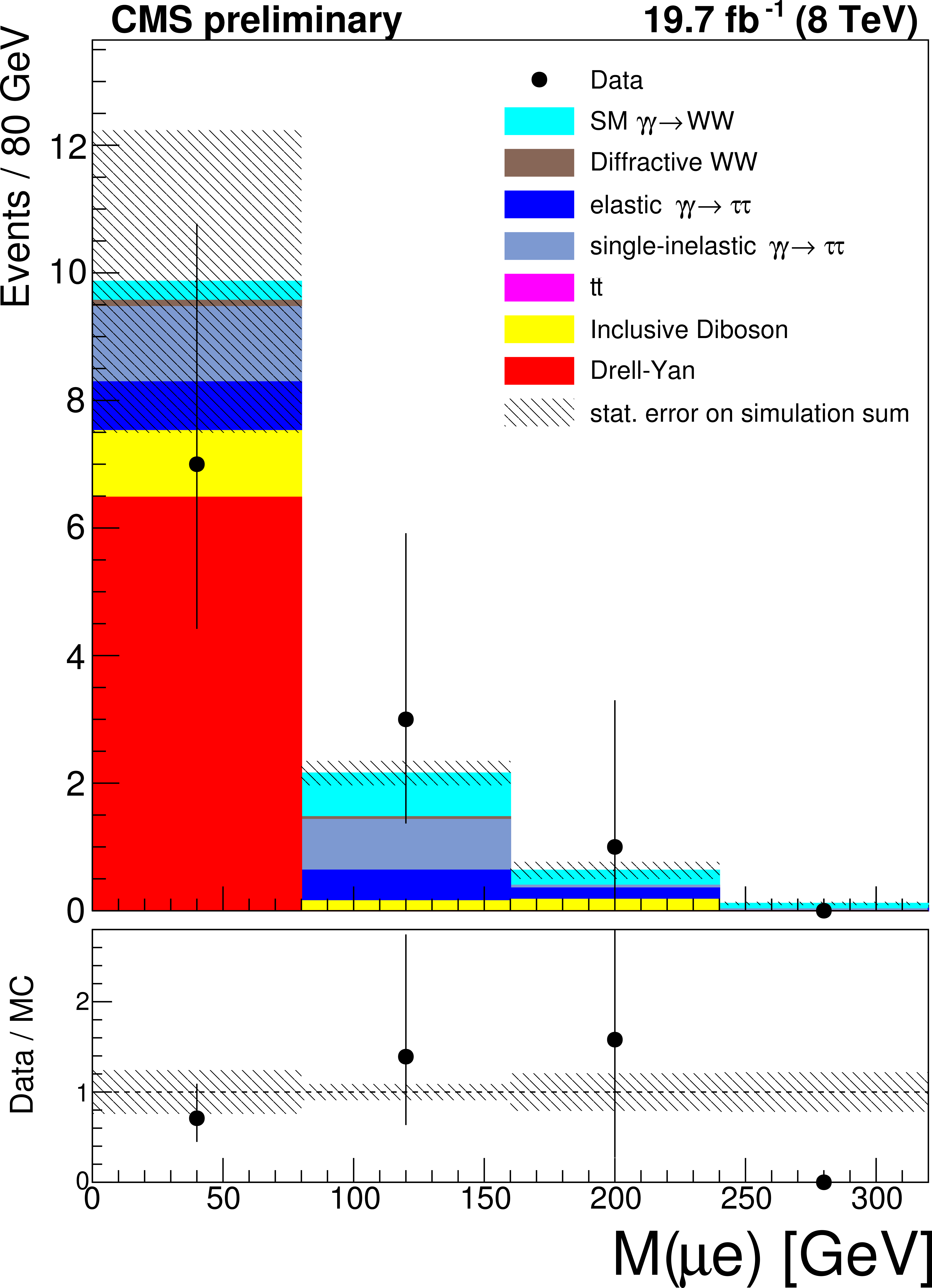
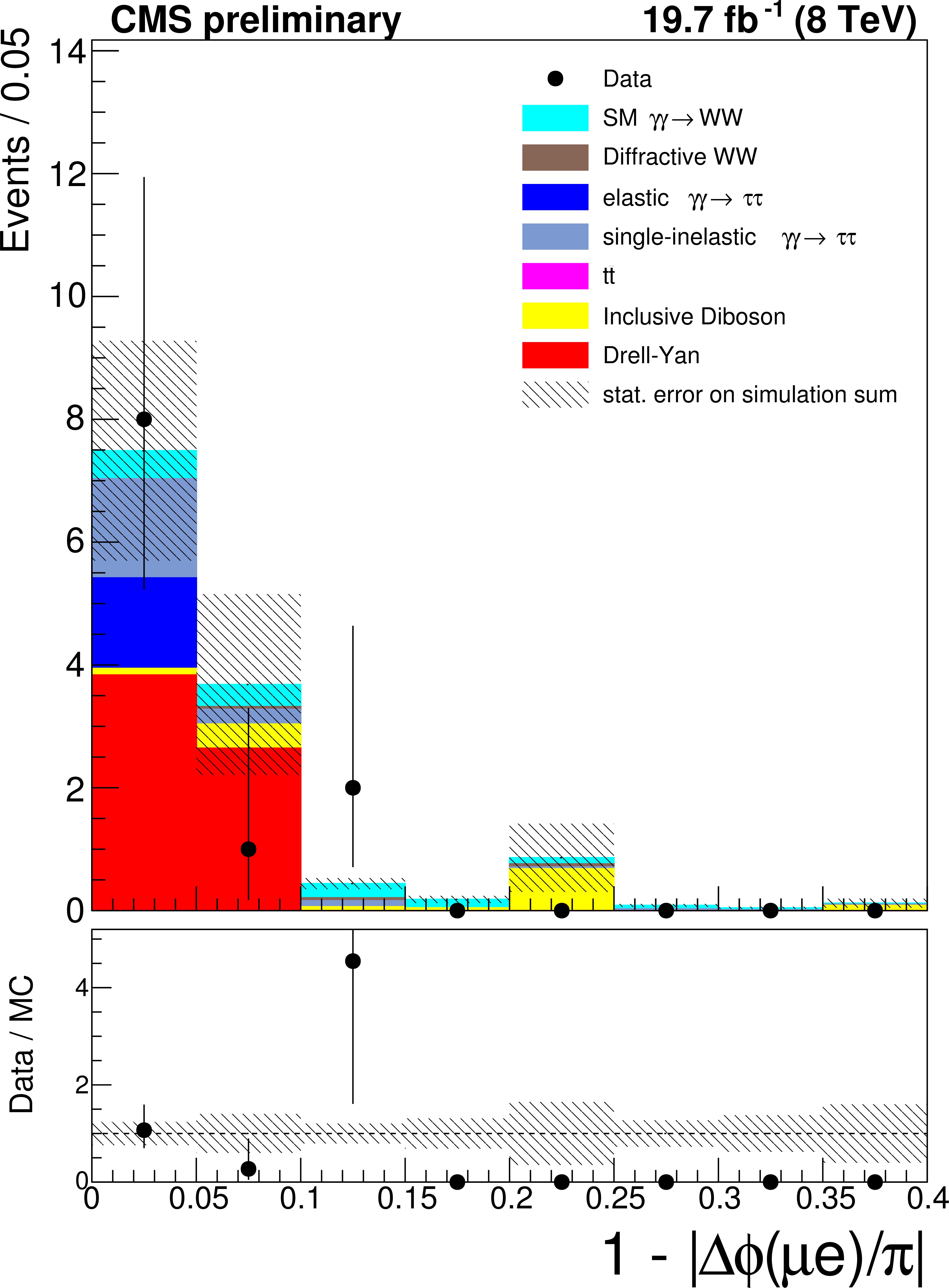
The $\mu ^{\pm }e^{\mp }$ invariant mass (a) and acoplanarity (b) are shown for data and the expected backgrounds for $p_{T}(\mu ^{\pm }e^{\mp }) < 30$ GeV and 0 extra tracks ($\gamma \gamma \to \tau ^{+}\tau ^{-}$ control region). The last bin in the acoplanarity distribution is an overflow bin and includes all events above acoplanarity 0.4. |
png ; pdf |
Figure 7-b:
The $\mu ^{\pm }e^{\mp }$ invariant mass (a) and acoplanarity (b) are shown for data and the expected backgrounds for $p_{T}(\mu ^{\pm }e^{\mp }) < 30$ GeV and 0 extra tracks ($\gamma \gamma \to \tau ^{+}\tau ^{-}$ control region). The last bin in the acoplanarity distribution is an overflow bin and includes all events above acoplanarity 0.4. |
png ; pdf |
Figure 8-a:
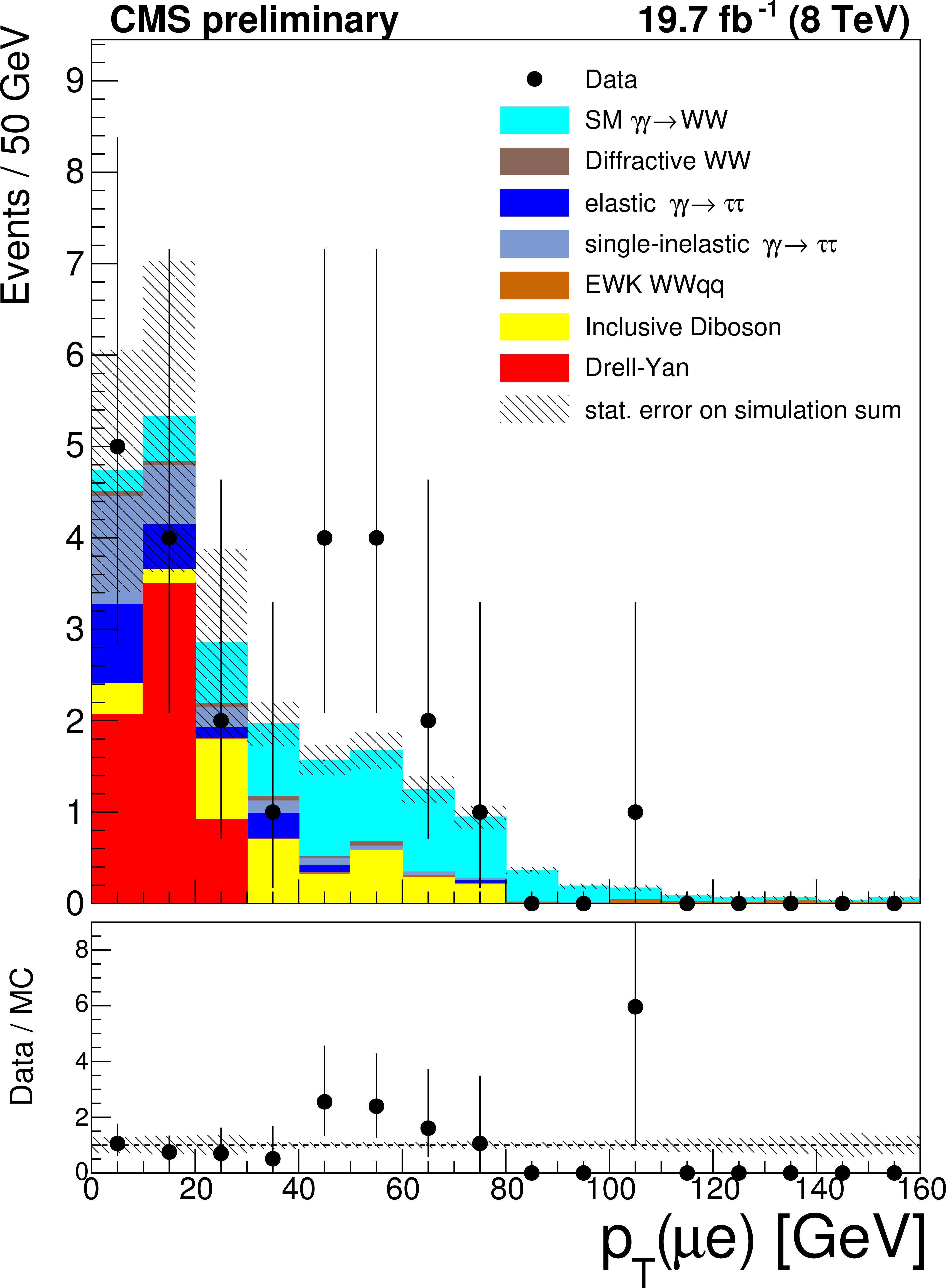
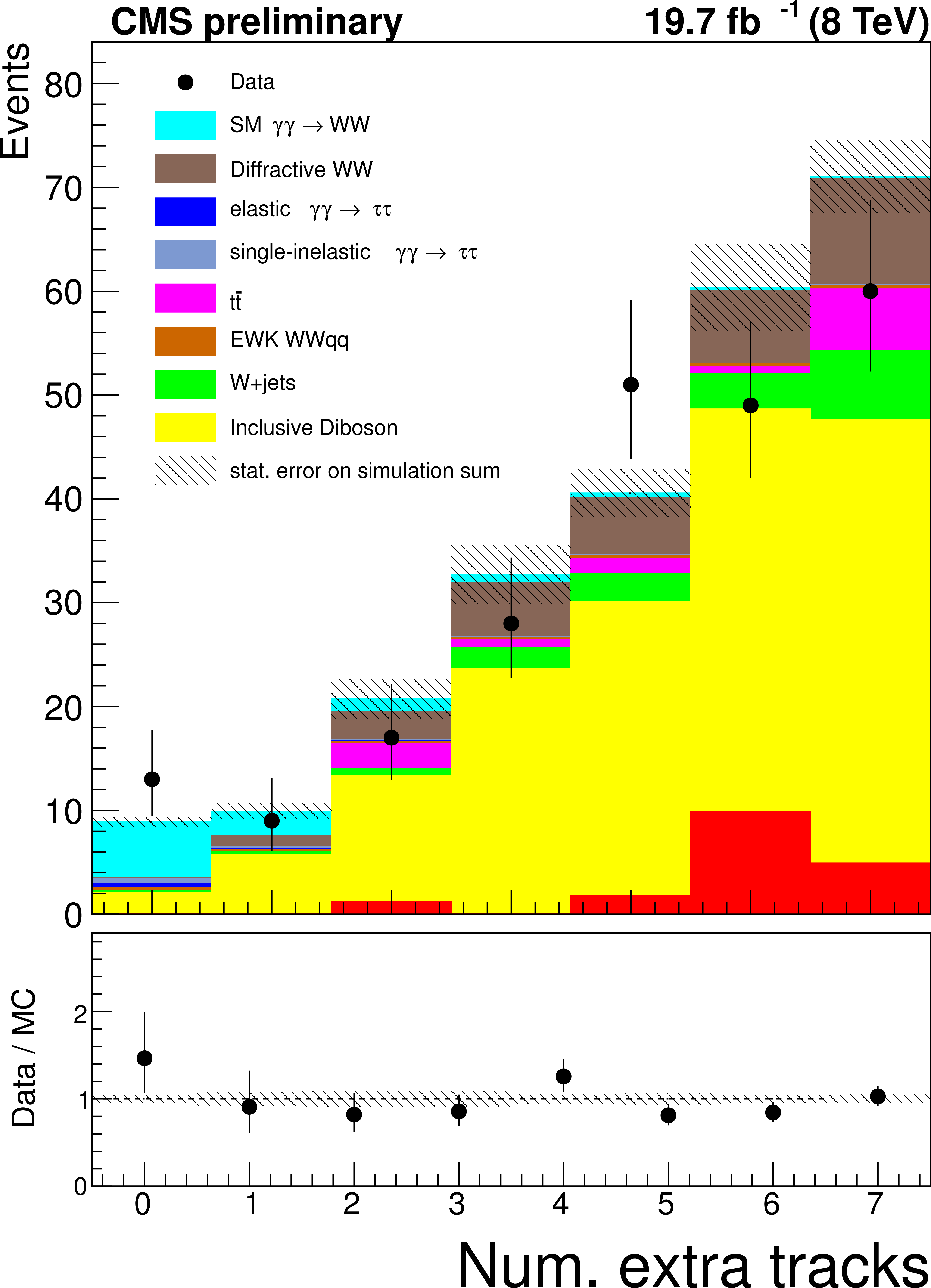
Muon-electron transverse momentum for events with zero associated tracks (a), and extra tracks multiplicity for events with $p_{T}(\mu ^{\pm }e^{\mp }) > 30$ GeV (b). The data is shown by points with error bars, the histograms indicate the expected SM signal and backgrounds. |
png ; pdf |
Figure 8-b:
Muon-electron transverse momentum for events with zero associated tracks (a), and extra tracks multiplicity for events with $p_{T}(\mu ^{\pm }e^{\mp }) > 30$ GeV (b). The data is shown by points with error bars, the histograms indicate the expected SM signal and backgrounds. |
png ; pdf |
Figure 9-a:
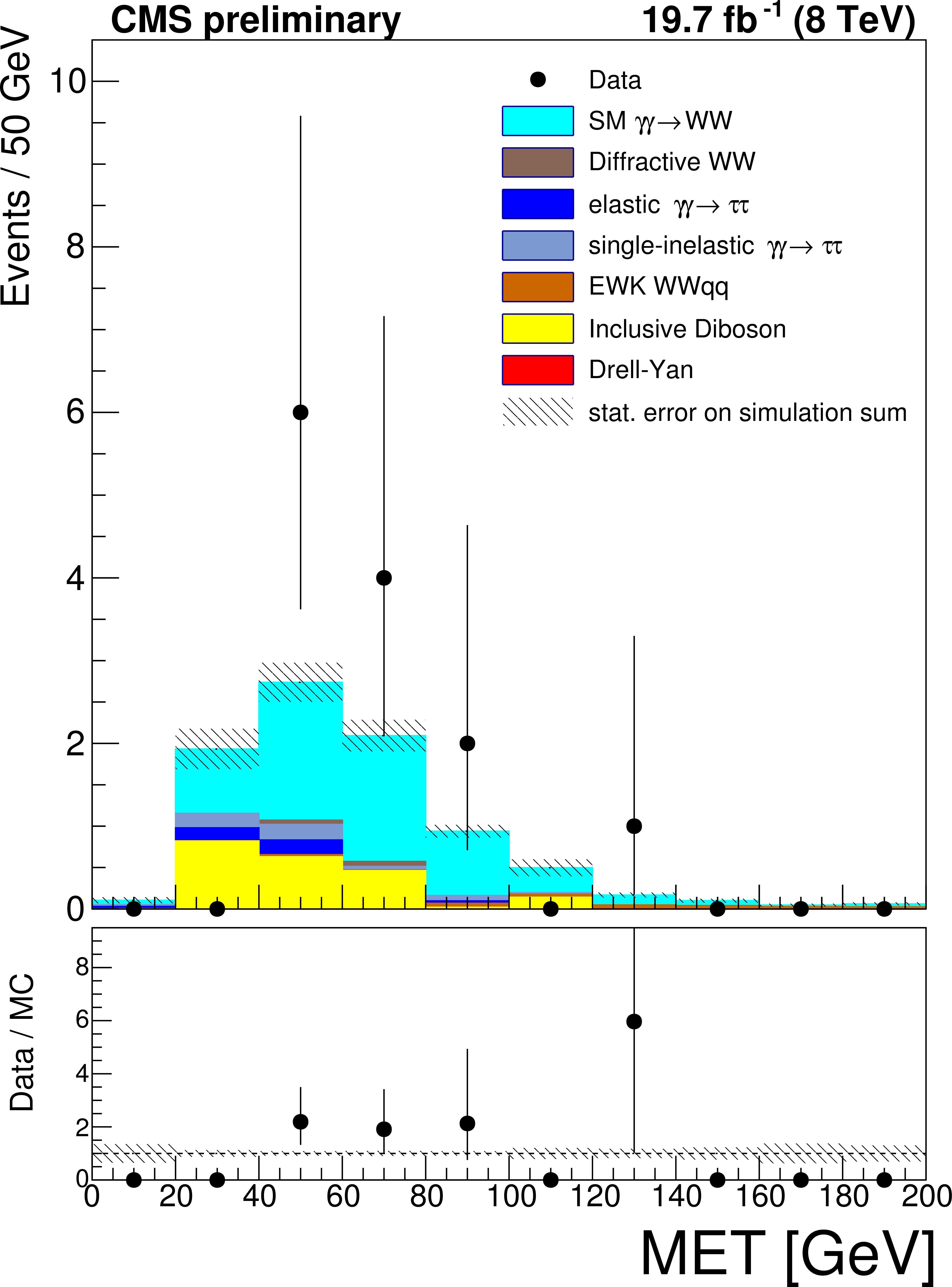
Muon-electron invariant mass (a), acoplanarity (b), and missing transverse energy (c) in the $\mathrm{ \gamma \gamma \to W^{+}W^{-} }$ signal region. The data is shown by points with error bars, the histograms indicate the expected SM signal and backgrounds. |
png ; pdf |
Figure 9-b:
Muon-electron invariant mass (a), acoplanarity (b), and missing transverse energy (c) in the $\mathrm{ \gamma \gamma \to W^{+}W^{-} }$ signal region. The data is shown by points with error bars, the histograms indicate the expected SM signal and backgrounds. |
png ; pdf |
Figure 9-c:
Muon-electron invariant mass (a), acoplanarity (b), and missing transverse energy (c) in the $\mathrm{ \gamma \gamma \to W^{+}W^{-} }$ signal region. The data is shown by points with error bars, the histograms indicate the expected SM signal and backgrounds. |
png ; pdf |
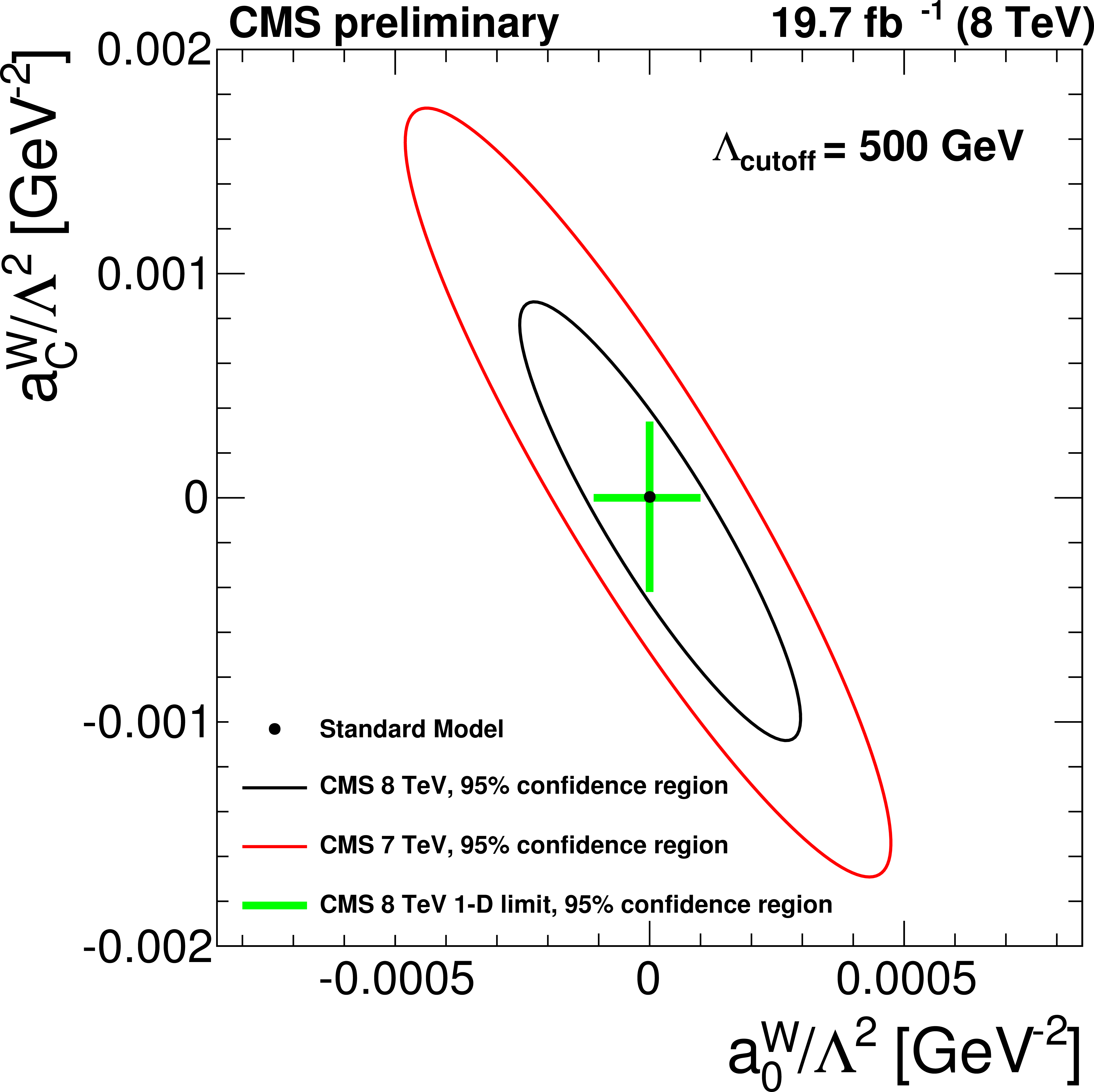
Figure 10:
Excluded values of the anomalous coupling parameters $a^{ {\mathrm {W}}}_{0}/\Lambda ^{2}$ and $a^{ {\mathrm {W}}}_{C}/\Lambda ^{2}$ with $\Lambda _{\text {cutoff}}=500$ GeV. The area outside the solid contour is excluded by this measurement at 95% CL. The predicted cross sections are rescaled to include the contribution from proton dissociation. |
|
|
Compact Muon Solenoid LHC, CERN |
|

|

|

|

|

|