

Compact Muon Solenoid
LHC, CERN
| CMS-PAS-FSQ-12-004 | ||
| Measurement of exclusive $\pi^{+} \pi^{-}$ production in proton-proton collisions at $\sqrt{s} =$ 7 TeV | ||
| CMS Collaboration | ||
| December 2015 | ||
| Abstract: We report a measurement of exclusive pion pair production in proton-proton collisions, dominated by $\mathrm{p} + \mathrm{p} \rightarrow \mathrm{p}^{(*)} + \pi^{+} \pi^{-} + \mathrm{p}^{(*)}$, where the $\pi^{+} \pi^{-}$ pair is produced at central rapidities $y$ and the incident protons stay intact or dissociate without being detected. The measurement is performed with the CMS detector at the LHC, using an integrated luminosity of 450 $\mu \mathrm{b}^{-1}$ collected at a center-of-mass energy of $\sqrt{s} =$ 7 TeV in 2010. The cross section measured in the phase space defined by $p_{T}(\pi) > $ 0.2 GeV/$c$ and $|y(\pi)| < $ 2 is 20.5 $\pm$ 0.3 (stat) $\pm$ 3.1 (syst) $\pm$ 0.8 (lumi) $\mu \mathrm{b}$. The differential $\pi^{+}\pi^{-}$ cross sections as a function of invariant mass, $p_{\mathrm{T}}$, and $y$, and the single $\pi$ cross section as a function of $p_{\mathrm{T}}$, are also shown and compared to model predictions. | ||
|
Links:
CDS record (PDF) ;
Public twiki page ;
CADI line (restricted) ;
These preliminary results are superseded in this paper, Superseded by FSQ-16-006. The superseded preliminary plots can be found here. |
||
| Figures | |
png ; pdf ; |
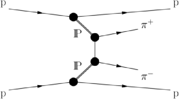
Figure 1-a:
(a) Double-Pomeron-Exchange (DPE) diagram producing a central $\pi ^{+}\pi ^{-}$ system in proton-proton collisions. (b) Photon-pomeron scattering producing exclusively a $\rho $-meson that subsequently decays into a pair of pions. |
png ; pdf ; |
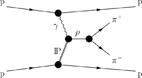
Figure 1-b:
(a) Double-Pomeron-Exchange (DPE) diagram producing a central $\pi ^{+}\pi ^{-}$ system in proton-proton collisions. (b) Photon-pomeron scattering producing exclusively a $\rho $-meson that subsequently decays into a pair of pions. |
png ; pdf ; |
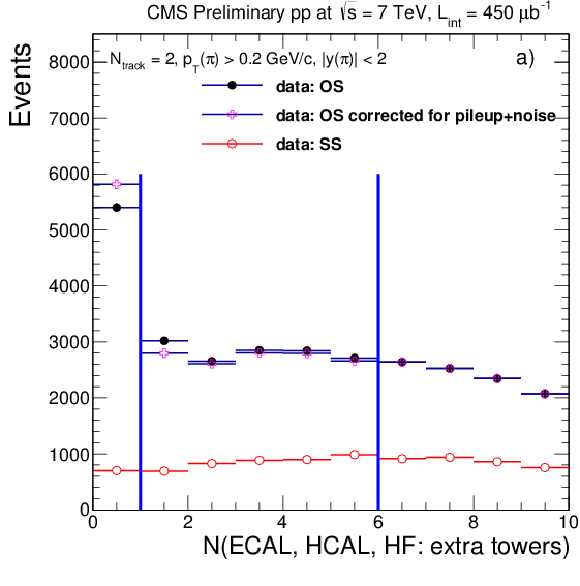
Figure 2-a:
(a) Distribution of ECAL+HCAL tower multiplicities above noise threshold in events with colliding beams and pairs of opposite-sign (OS) and same-sign (SS) tracks reconstructed. The distribution after the pileup correction is shown by crosses. The vertical blue lines indicate the background control region. (b) Distribution of ECAL+HCAL tower multiplicities above the noise thresholds in the Zero-Bias sample with no tracks required, normalized to unity. |
png ; pdf ; |
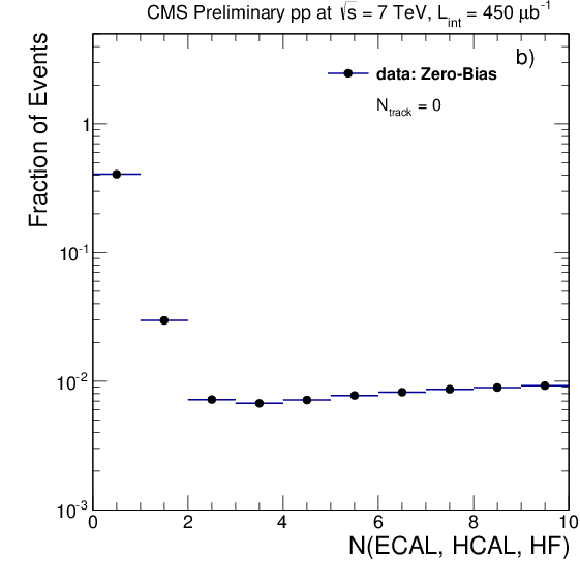
Figure 2-b:
(a) Distribution of ECAL+HCAL tower multiplicities above noise threshold in events with colliding beams and pairs of opposite-sign (OS) and same-sign (SS) tracks reconstructed. The distribution after the pileup correction is shown by crosses. The vertical blue lines indicate the background control region. (b) Distribution of ECAL+HCAL tower multiplicities above the noise thresholds in the Zero-Bias sample with no tracks required, normalized to unity. |
png ; pdf ; |
Figure 3-a:
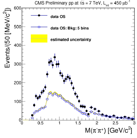
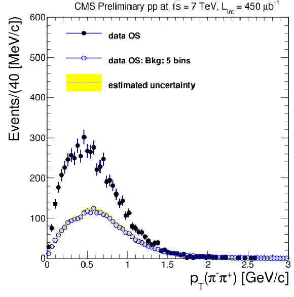
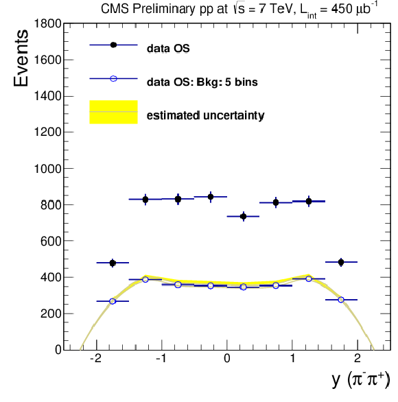
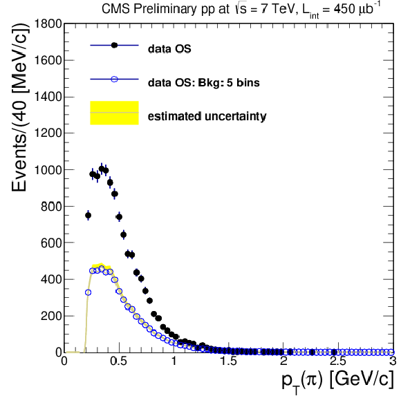
Detector-level distributions in opposite-sign events after all analysis selections (points with error bars) after pileup migration correction, compared with the background estimated from the control region in data (open points). The invariant mass spectrum (a), pion-pair $p_{\mathrm{T}}$ (b), pion-pair rapidity (c), and single pion $p_{\mathrm{T}}$ (d) are shown. The yellow band indicates the range of the background estimate when varying the size of the control regions from 1 extra tower to 2-7 extra towers. |
png ; pdf ; |
Figure 3-b:
Detector-level distributions in opposite-sign events after all analysis selections (points with error bars) after pileup migration correction, compared with the background estimated from the control region in data (open points). The invariant mass spectrum (a), pion-pair $p_{\mathrm{T}}$ (b), pion-pair rapidity (c), and single pion $p_{\mathrm{T}}$ (d) are shown. The yellow band indicates the range of the background estimate when varying the size of the control regions from 1 extra tower to 2-7 extra towers. |
png ; pdf ; |
Figure 3-c:
Detector-level distributions in opposite-sign events after all analysis selections (points with error bars) after pileup migration correction, compared with the background estimated from the control region in data (open points). The invariant mass spectrum (a), pion-pair $p_{\mathrm{T}}$ (b), pion-pair rapidity (c), and single pion $p_{\mathrm{T}}$ (d) are shown. The yellow band indicates the range of the background estimate when varying the size of the control regions from 1 extra tower to 2-7 extra towers. |
png ; pdf ; |
Figure 3-d:
Detector-level distributions in opposite-sign events after all analysis selections (points with error bars) after pileup migration correction, compared with the background estimated from the control region in data (open points). The invariant mass spectrum (a), pion-pair $p_{\mathrm{T}}$ (b), pion-pair rapidity (c), and single pion $p_{\mathrm{T}}$ (d) are shown. The yellow band indicates the range of the background estimate when varying the size of the control regions from 1 extra tower to 2-7 extra towers. |
png ; pdf ; |
Figure 4-a:
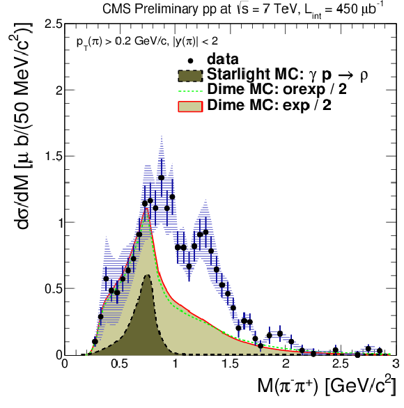
Corrected differential cross sections for $ \mathrm{ p p } \rightarrow p^{(*)} + \pi ^{+}\pi ^{-} + \mathrm{ p }^{(*)}$, compared to the stacked predictions of DPE production from the \textsc {Dime MC} (solid curve) and $\rho $ photoproduction from \textsc {starlight} (dashed curve). The shaded band shows the overall systematic uncertainty, and the thin error bar indicates the statistical uncertainty. The results are plotted on a linear scale (a) and a logarithmic scale (b). |
png ; pdf ; |
Figure 4-b:
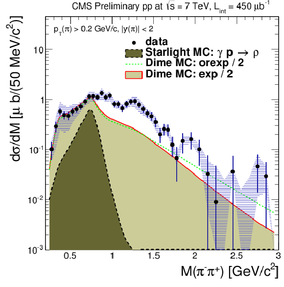
Corrected differential cross sections for $ \mathrm{ p p } \rightarrow p^{(*)} + \pi ^{+}\pi ^{-} + \mathrm{ p }^{(*)}$, compared to the stacked predictions of DPE production from the \textsc {Dime MC} (solid curve) and $\rho $ photoproduction from \textsc {starlight} (dashed curve). The shaded band shows the overall systematic uncertainty, and the thin error bar indicates the statistical uncertainty. The results are plotted on a linear scale (a) and a logarithmic scale (b). |
png ; pdf ; |
Figure 5-a:
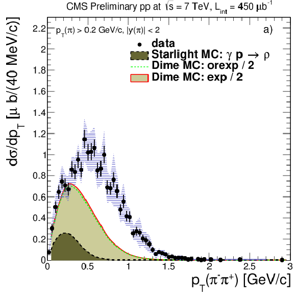
Corrected differential cross sections for $ \mathrm{ p p } \rightarrow p^{(*)} + \pi ^{+}\pi ^{-} + \mathrm{ p }^{(*)}$, compared to the stacked predictions of DPE production from the \textsc {Dime MC} (solid curve), and $\rho $ photoproduction from \textsc {starlight} (dashed curve). The pion pair $p_{\mathrm{T}}$ (a, b) and pion pair rapidity (c, d) , and single pion $p_{\mathrm{ T } }$ (e, f) are shown. The shaded band shows the overall systematic uncertainty, and the thin error bar indicates the statistical uncertainties. The results are plotted on a linear scale (a,c) and a logarithmic scale (b,d). |
png ; pdf ; |
Figure 5-b:
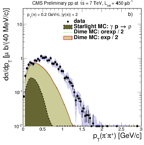
Corrected differential cross sections for $ \mathrm{ p p } \rightarrow p^{(*)} + \pi ^{+}\pi ^{-} + \mathrm{ p }^{(*)}$, compared to the stacked predictions of DPE production from the \textsc {Dime MC} (solid curve), and $\rho $ photoproduction from \textsc {starlight} (dashed curve). The pion pair $p_{\mathrm{T}}$ (a, b) and pion pair rapidity (c, d) , and single pion $p_{\mathrm{ T } }$ (e, f) are shown. The shaded band shows the overall systematic uncertainty, and the thin error bar indicates the statistical uncertainties. The results are plotted on a linear scale (a,c) and a logarithmic scale (b,d). |
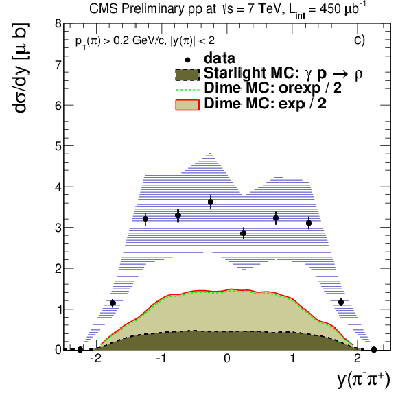
png ; pdf ; |
Figure 5-c:
Corrected differential cross sections for $ \mathrm{ p p } \rightarrow p^{(*)} + \pi ^{+}\pi ^{-} + \mathrm{ p }^{(*)}$, compared to the stacked predictions of DPE production from the \textsc {Dime MC} (solid curve), and $\rho $ photoproduction from \textsc {starlight} (dashed curve). The pion pair $p_{\mathrm{T}}$ (a, b) and pion pair rapidity (c, d) , and single pion $p_{\mathrm{ T } }$ (e, f) are shown. The shaded band shows the overall systematic uncertainty, and the thin error bar indicates the statistical uncertainties. The results are plotted on a linear scale (a,c) and a logarithmic scale (b,d). |
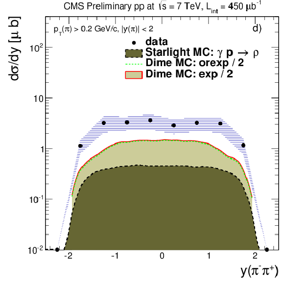
png ; pdf ; |
Figure 5-d:
Corrected differential cross sections for $ \mathrm{ p p } \rightarrow p^{(*)} + \pi ^{+}\pi ^{-} + \mathrm{ p }^{(*)}$, compared to the stacked predictions of DPE production from the \textsc {Dime MC} (solid curve), and $\rho $ photoproduction from \textsc {starlight} (dashed curve). The pion pair $p_{\mathrm{T}}$ (a, b) and pion pair rapidity (c, d) , and single pion $p_{\mathrm{ T } }$ (e, f) are shown. The shaded band shows the overall systematic uncertainty, and the thin error bar indicates the statistical uncertainties. The results are plotted on a linear scale (a,c) and a logarithmic scale (b,d). |
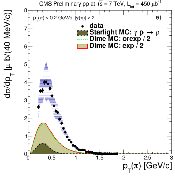
png ; pdf ; |
Figure 5-e:
Corrected differential cross sections for $ \mathrm{ p p } \rightarrow p^{(*)} + \pi ^{+}\pi ^{-} + \mathrm{ p }^{(*)}$, compared to the stacked predictions of DPE production from the \textsc {Dime MC} (solid curve), and $\rho $ photoproduction from \textsc {starlight} (dashed curve). The pion pair $p_{\mathrm{T}}$ (a, b) and pion pair rapidity (c, d) , and single pion $p_{\mathrm{ T } }$ (e, f) are shown. The shaded band shows the overall systematic uncertainty, and the thin error bar indicates the statistical uncertainties. The results are plotted on a linear scale (a,c) and a logarithmic scale (b,d). |
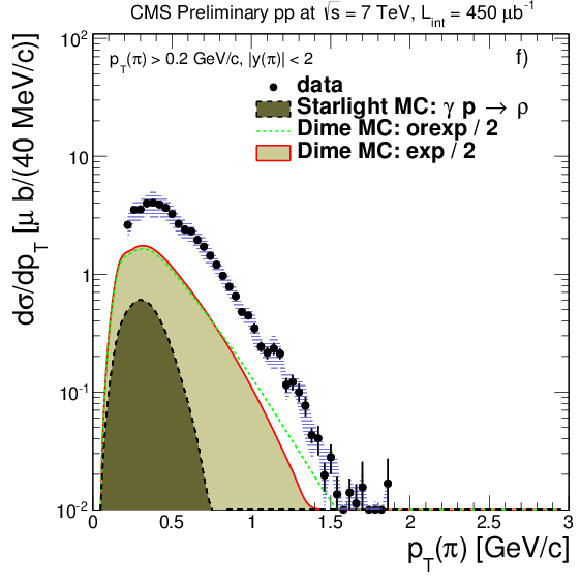
png ; pdf ; |
Figure 5-f:
Corrected differential cross sections for $ \mathrm{ p p } \rightarrow p^{(*)} + \pi ^{+}\pi ^{-} + \mathrm{ p }^{(*)}$, compared to the stacked predictions of DPE production from the \textsc {Dime MC} (solid curve), and $\rho $ photoproduction from \textsc {starlight} (dashed curve). The pion pair $p_{\mathrm{T}}$ (a, b) and pion pair rapidity (c, d) , and single pion $p_{\mathrm{ T } }$ (e, f) are shown. The shaded band shows the overall systematic uncertainty, and the thin error bar indicates the statistical uncertainties. The results are plotted on a linear scale (a,c) and a logarithmic scale (b,d). |
png ; pdf ; |
Figure 6-a:
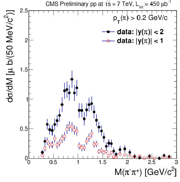
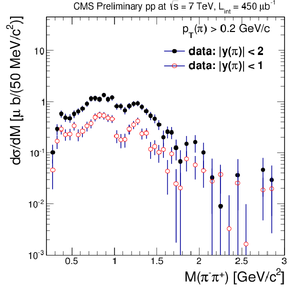
Corrected differential cross sections for $ \mathrm{ p p } \rightarrow p^{(*)} + \pi ^{+}\pi ^{-} + p^{(*)}$, comparing in the two $|y|$ regions $<$ 1 and $< $ 2. The results are plotted on a linear scale (a) and a logarithmic scale (b). |
png ; pdf ; |
Figure 6-b:
Corrected differential cross sections for $ \mathrm{ p p } \rightarrow p^{(*)} + \pi ^{+}\pi ^{-} + p^{(*)}$, comparing in the two $|y|$ regions $<$ 1 and $< $ 2. The results are plotted on a linear scale (a) and a logarithmic scale (b). |

|
Compact Muon Solenoid LHC, CERN |

|

|

|

|

|

|