

Compact Muon Solenoid
LHC, CERN
| CMS-PAS-FSQ-12-001 | ||
| Dijet production with a large rapidity gap between the jets | ||
| CMS Collaboration | ||
| June 2015 | ||
| Abstract: Events with no particles produced between two leading jets have been studied in pp collisions at $\sqrt{s} =$ 7 TeV, for jets with $p_{\mathrm{T}} >$ 40 GeV and 1.5 $< |\eta| <$ 4.5, reconstructed in opposite hemispheres of the detector. The ratio of the yield for these large rapidity gap events to that for inclusive dijet events has been measured as a function of the transverse momentum of the second-leading jet and the size of the pseudorapidity interval between the jets. The observed excess of events with no charged particles between the jets is consistent with the presence of hard color-singlet exchange. The measurement is based on 8 pb$^{-1}$ of integrated luminosity collected with the CMS detector in 2010. | ||
|
Links:
CDS record (PDF) ;
Public twiki page ;
CADI line (restricted) ; Figures are also available from the CDS record. These preliminary results are superseded in this paper, EPJC 78 (2018) 242 [Erratum: EPJC 80 (2020) 441]. The superseded preliminary plots can be found here. |
||
| Figures | |
png ; pdf |
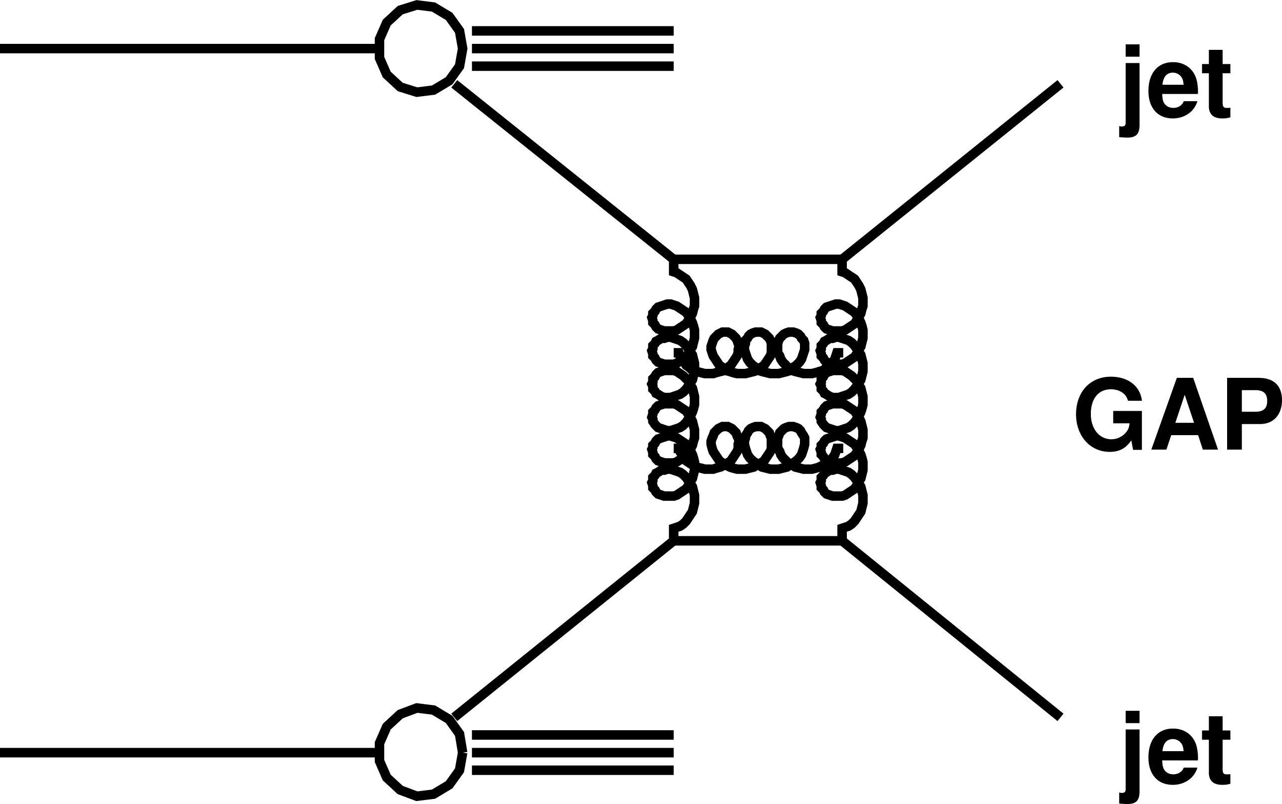
Figure 1:
Schematic diagram of a dijet event with a rapidity gap between the jets (jet--gap--jet event).The gap is defined as the absence of charged particle tracks above a $p_\mathrm {T}$ threshold. |
png ; pdf |
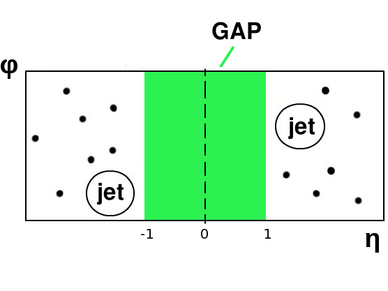
Figure 2:
Schematic picture of a jet-gap-jet event in the $\varphi $ vs. $\eta $ plane. The circles indicate the two jets reconstructed on each side of the detector, and the shaded area represents the region of the potential rapidity gap, in which the charged multiplicity is measured. |
png ; pdf |
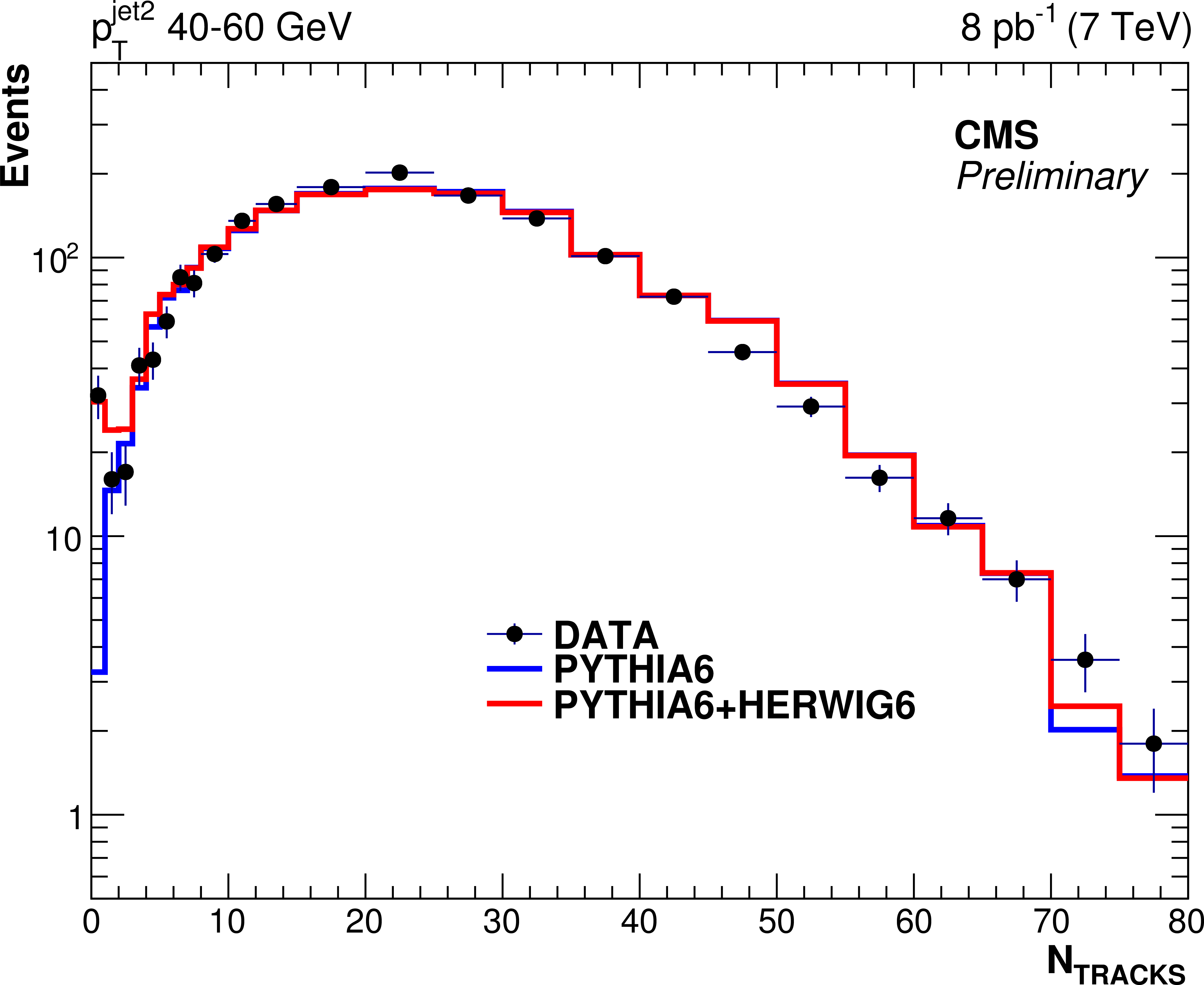
Figure 3-a:
Charged multiplicity distributions for $ {p_{\mathrm {T}}} ^\mathrm {jet2}$ 40-60 GeV, 60-100 GeV and 100-200 GeV, compared to predictions of PYTHIA6 and HERWIG6. The normalization of the MC distributions in each $ {p_{\mathrm {T}}} ^\mathrm {jet2}$ bin is obtained from a fit to the data. |
png ; pdf |
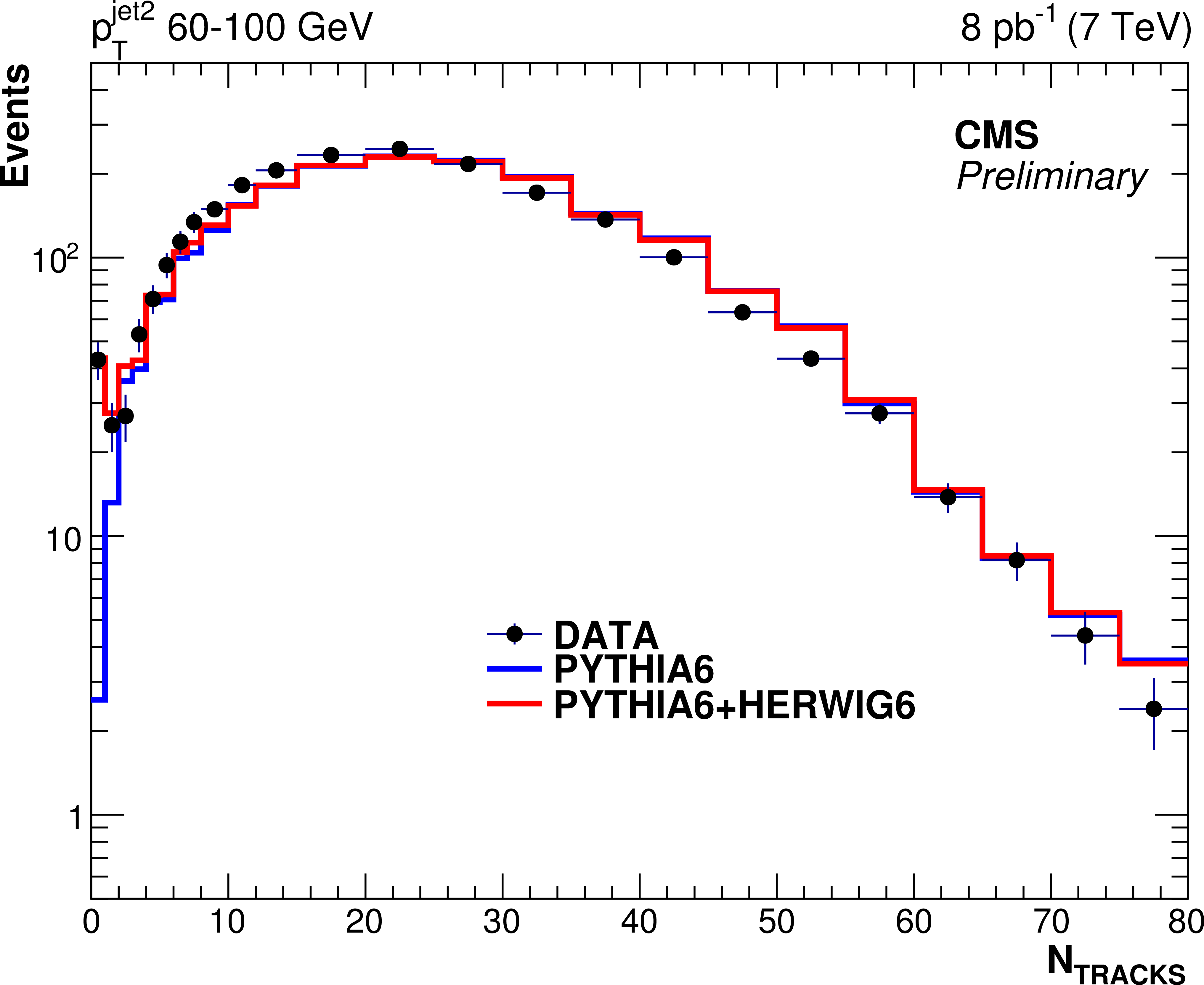
Figure 3-b:
Charged multiplicity distributions for $ {p_{\mathrm {T}}} ^\mathrm {jet2}$ 40-60 GeV, 60-100 GeV and 100-200 GeV, compared to predictions of PYTHIA6 and HERWIG6. The normalization of the MC distributions in each $ {p_{\mathrm {T}}} ^\mathrm {jet2}$ bin is obtained from a fit to the data. |
png ; pdf |
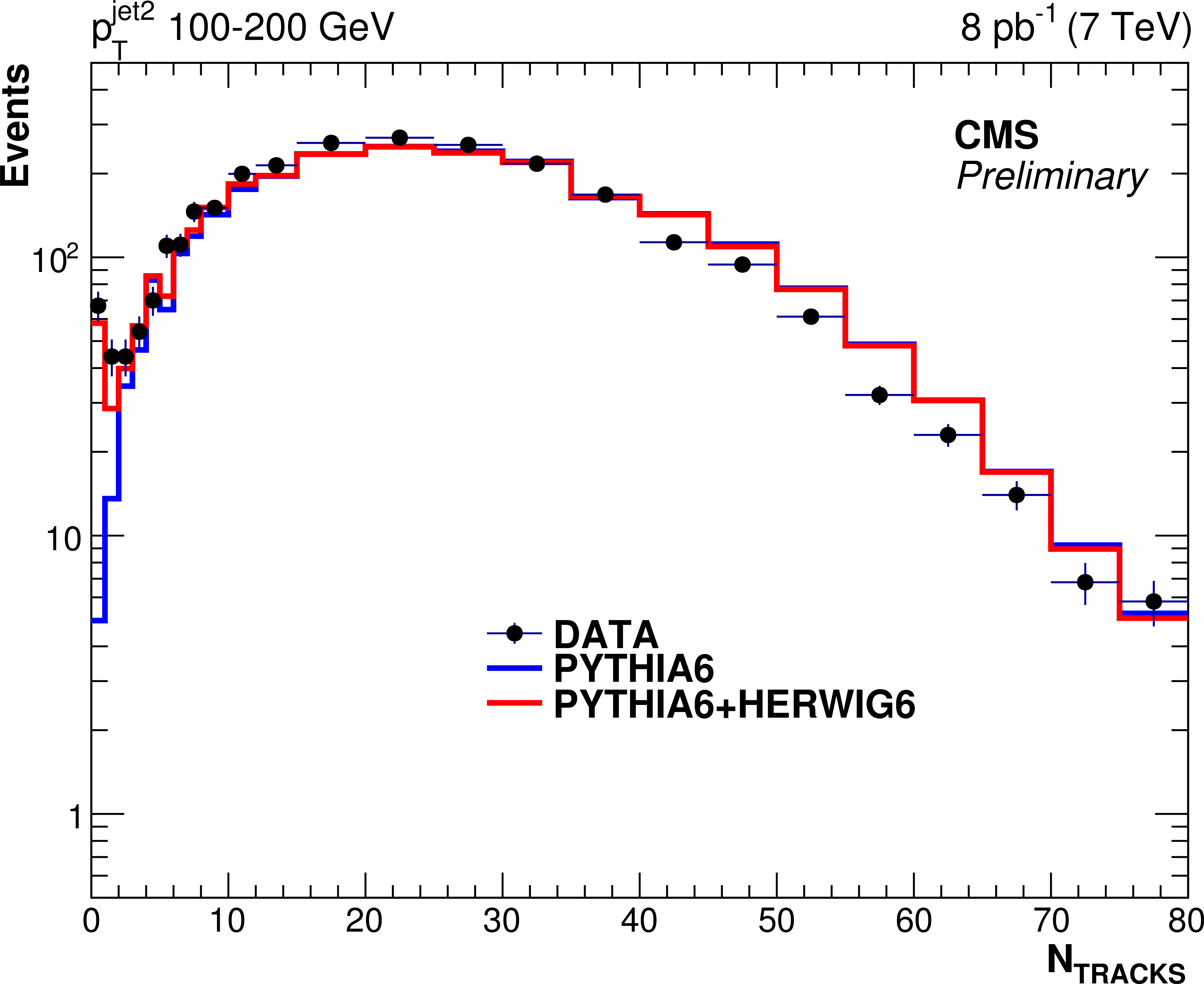
Figure 3-c:
Charged multiplicity distributions for $ {p_{\mathrm {T}}} ^\mathrm {jet2}$ 40-60 GeV, 60-100 GeV and 100-200 GeV, compared to predictions of PYTHIA6 and HERWIG6. The normalization of the MC distributions in each $ {p_{\mathrm {T}}} ^\mathrm {jet2}$ bin is obtained from a fit to the data. |
png ; pdf |
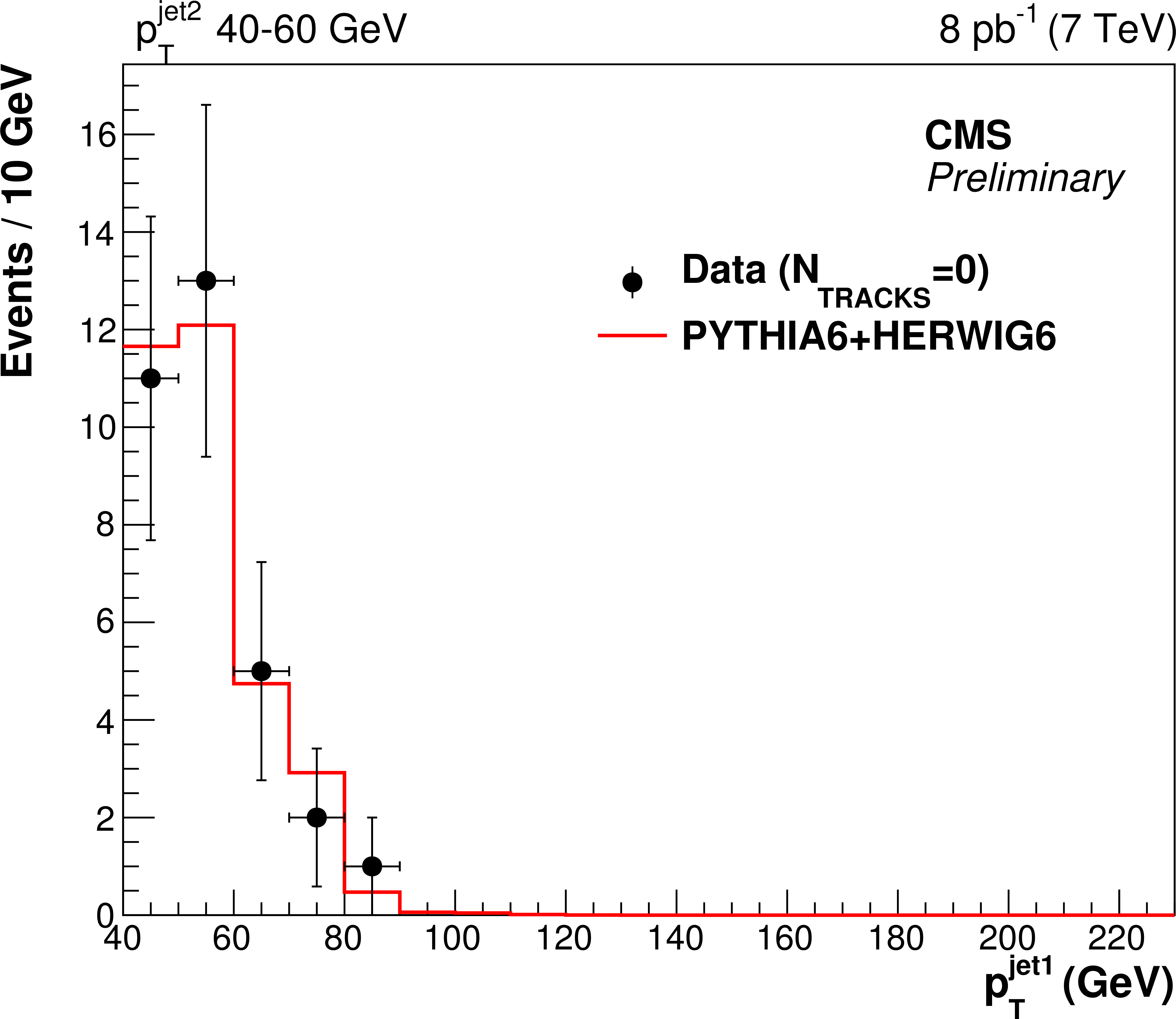
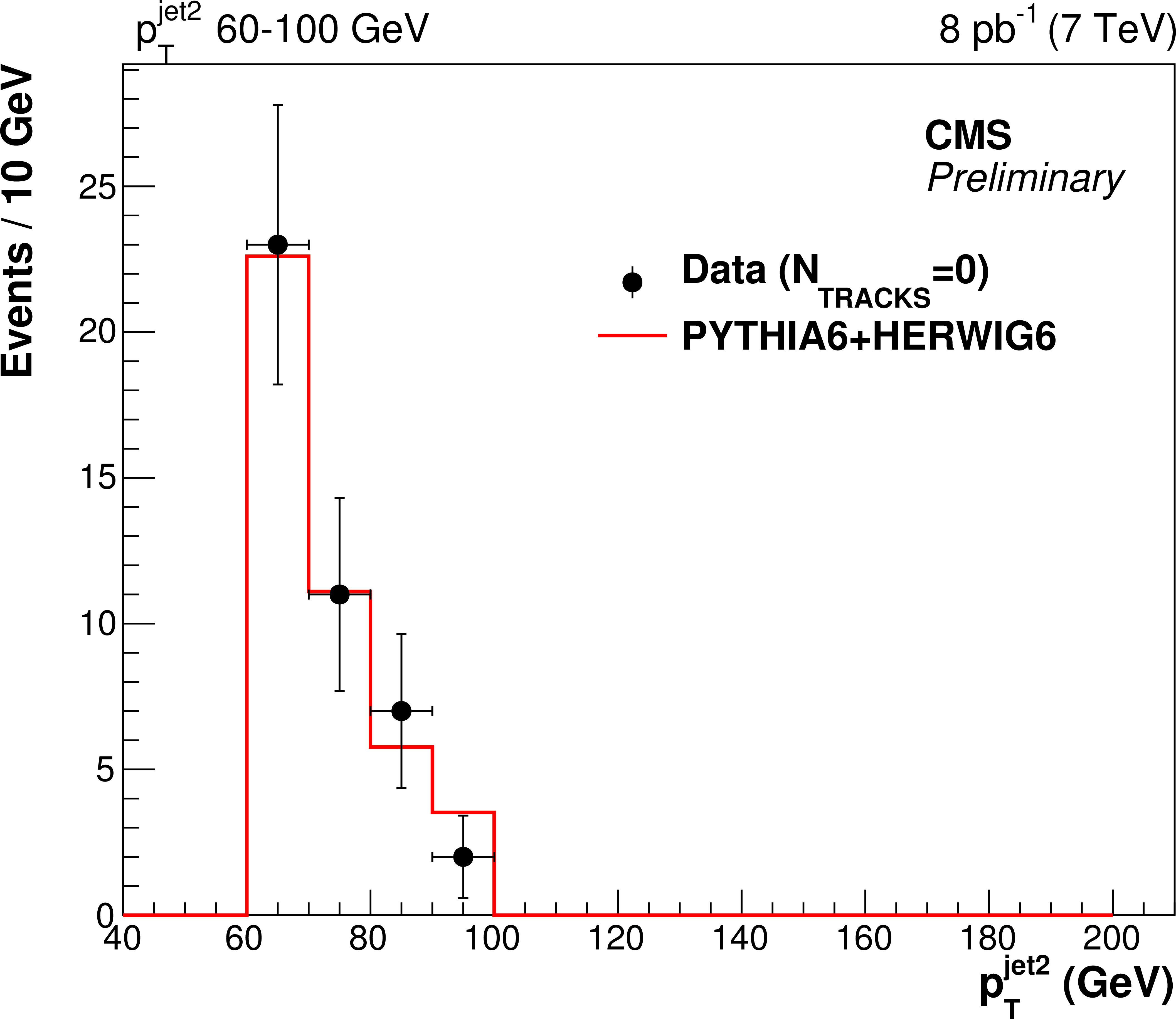
Figure 4-a:
Distributions of the leading jet (a,c,e) and the second-leading jet (b,d,f) $ {p_{\mathrm {T}}} $ for the three dijet samples with $40< {p_{\mathrm {T}}} ^\mathrm {jet2}<60$ GeV (a,b), $60< {p_{\mathrm {T}}} ^\mathrm {jet2}<100$ GeV (c,d), and $100< {p_{\mathrm {T}}} ^\mathrm {jet2}<200$ GeV (e,f) after all selections, for events with no tracks reconstructed in the rapidity gap region $|\eta |<1$, compared to MC predictions. The error bars indicate the statistical uncertainty. The normalization of the MC samples is obtained from a fit to the data from Fig. 3. |
png ; pdf |
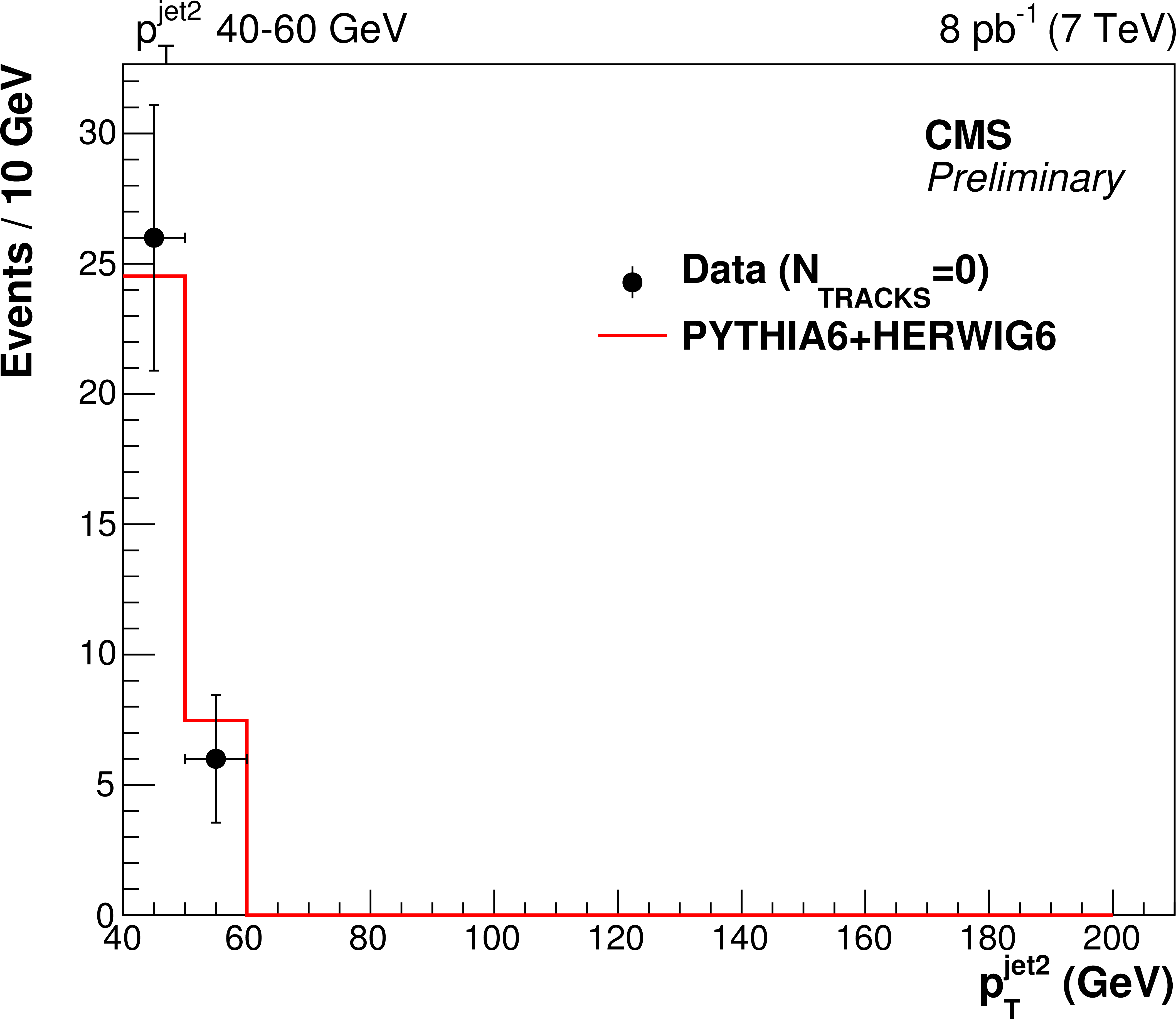
Figure 4-b:
Distributions of the leading jet (a,c,e) and the second-leading jet (b,d,f) $ {p_{\mathrm {T}}} $ for the three dijet samples with $40< {p_{\mathrm {T}}} ^\mathrm {jet2}<60$ GeV (a,b), $60< {p_{\mathrm {T}}} ^\mathrm {jet2}<100$ GeV (c,d), and $100< {p_{\mathrm {T}}} ^\mathrm {jet2}<200$ GeV (e,f) after all selections, for events with no tracks reconstructed in the rapidity gap region $|\eta |<1$, compared to MC predictions. The error bars indicate the statistical uncertainty. The normalization of the MC samples is obtained from a fit to the data from Fig. 3. |
png ; pdf |
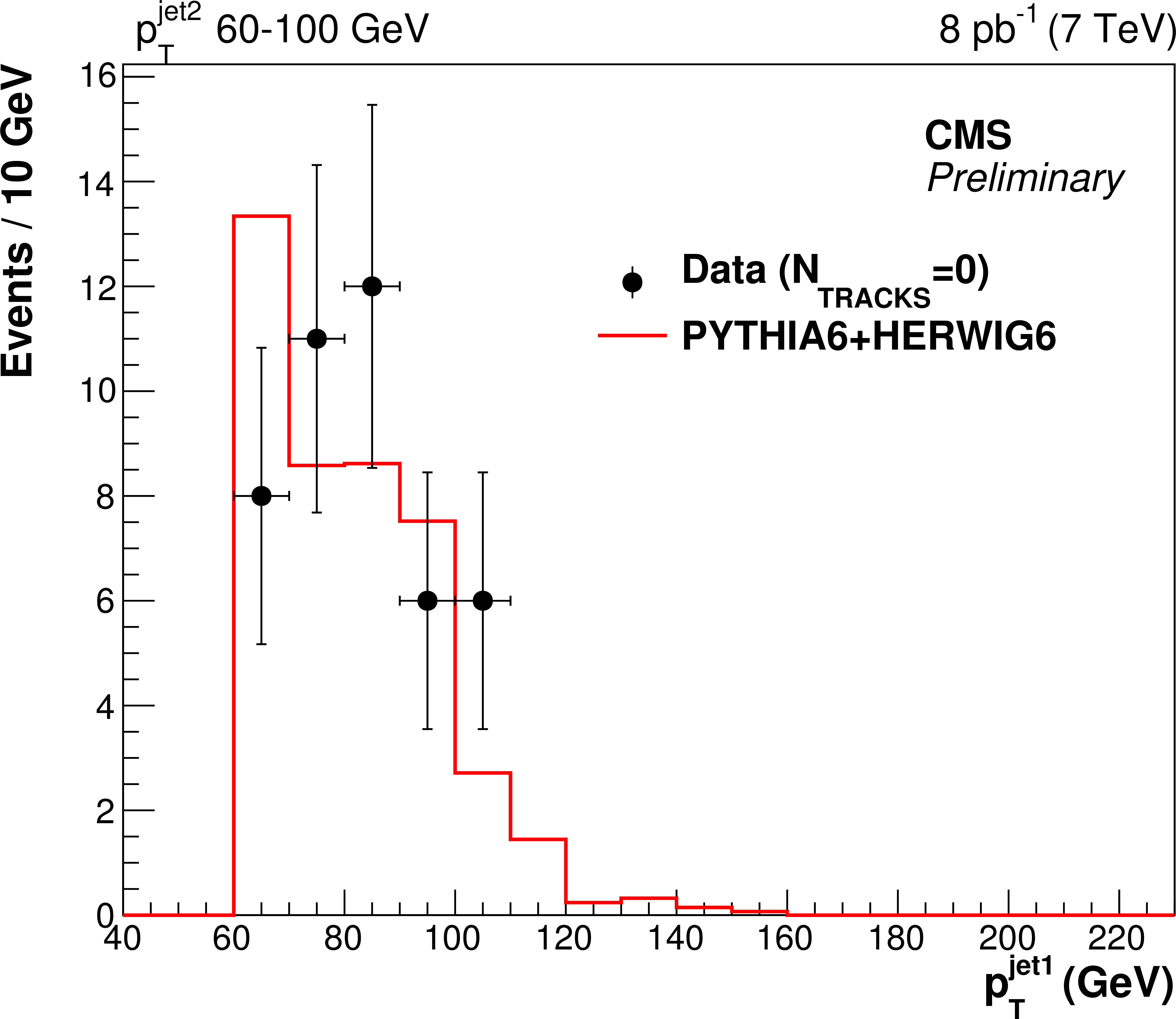
Figure 4-c:
Distributions of the leading jet (a,c,e) and the second-leading jet (b,d,f) $ {p_{\mathrm {T}}} $ for the three dijet samples with $40< {p_{\mathrm {T}}} ^\mathrm {jet2}<60$ GeV (a,b), $60< {p_{\mathrm {T}}} ^\mathrm {jet2}<100$ GeV (c,d), and $100< {p_{\mathrm {T}}} ^\mathrm {jet2}<200$ GeV (e,f) after all selections, for events with no tracks reconstructed in the rapidity gap region $|\eta |<1$, compared to MC predictions. The error bars indicate the statistical uncertainty. The normalization of the MC samples is obtained from a fit to the data from Fig. 3. |
png ; pdf |
Figure 4-d:
Distributions of the leading jet (a,c,e) and the second-leading jet (b,d,f) $ {p_{\mathrm {T}}} $ for the three dijet samples with $40< {p_{\mathrm {T}}} ^\mathrm {jet2}<60$ GeV (a,b), $60< {p_{\mathrm {T}}} ^\mathrm {jet2}<100$ GeV (c,d), and $100< {p_{\mathrm {T}}} ^\mathrm {jet2}<200$ GeV (e,f) after all selections, for events with no tracks reconstructed in the rapidity gap region $|\eta |<1$, compared to MC predictions. The error bars indicate the statistical uncertainty. The normalization of the MC samples is obtained from a fit to the data from Fig. 3. |
png ; pdf |
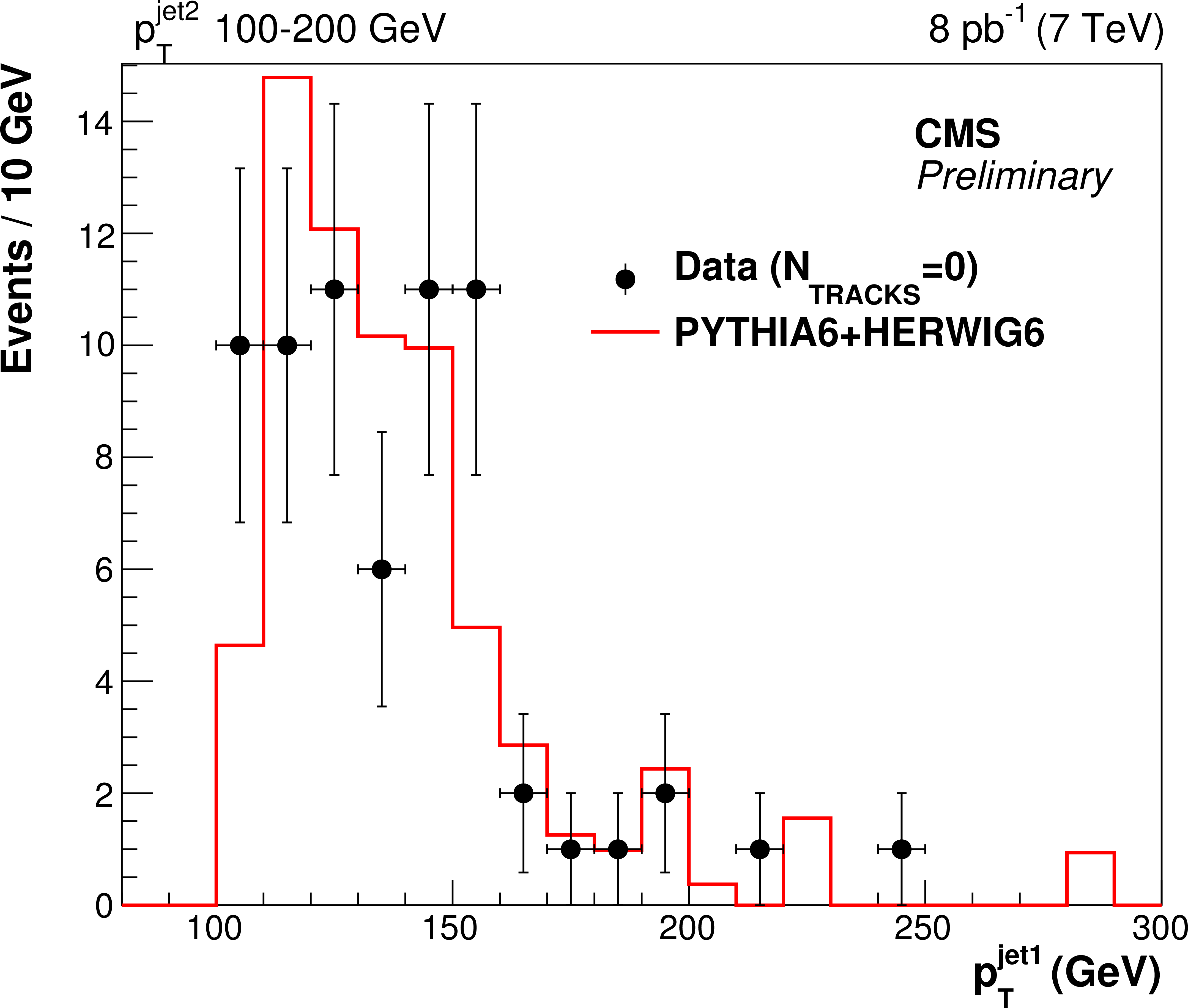
Figure 4-e:
Distributions of the leading jet (a,c,e) and the second-leading jet (b,d,f) $ {p_{\mathrm {T}}} $ for the three dijet samples with $40< {p_{\mathrm {T}}} ^\mathrm {jet2}<60$ GeV (a,b), $60< {p_{\mathrm {T}}} ^\mathrm {jet2}<100$ GeV (c,d), and $100< {p_{\mathrm {T}}} ^\mathrm {jet2}<200$ GeV (e,f) after all selections, for events with no tracks reconstructed in the rapidity gap region $|\eta |<1$, compared to MC predictions. The error bars indicate the statistical uncertainty. The normalization of the MC samples is obtained from a fit to the data from Fig. 3. |
png ; pdf |
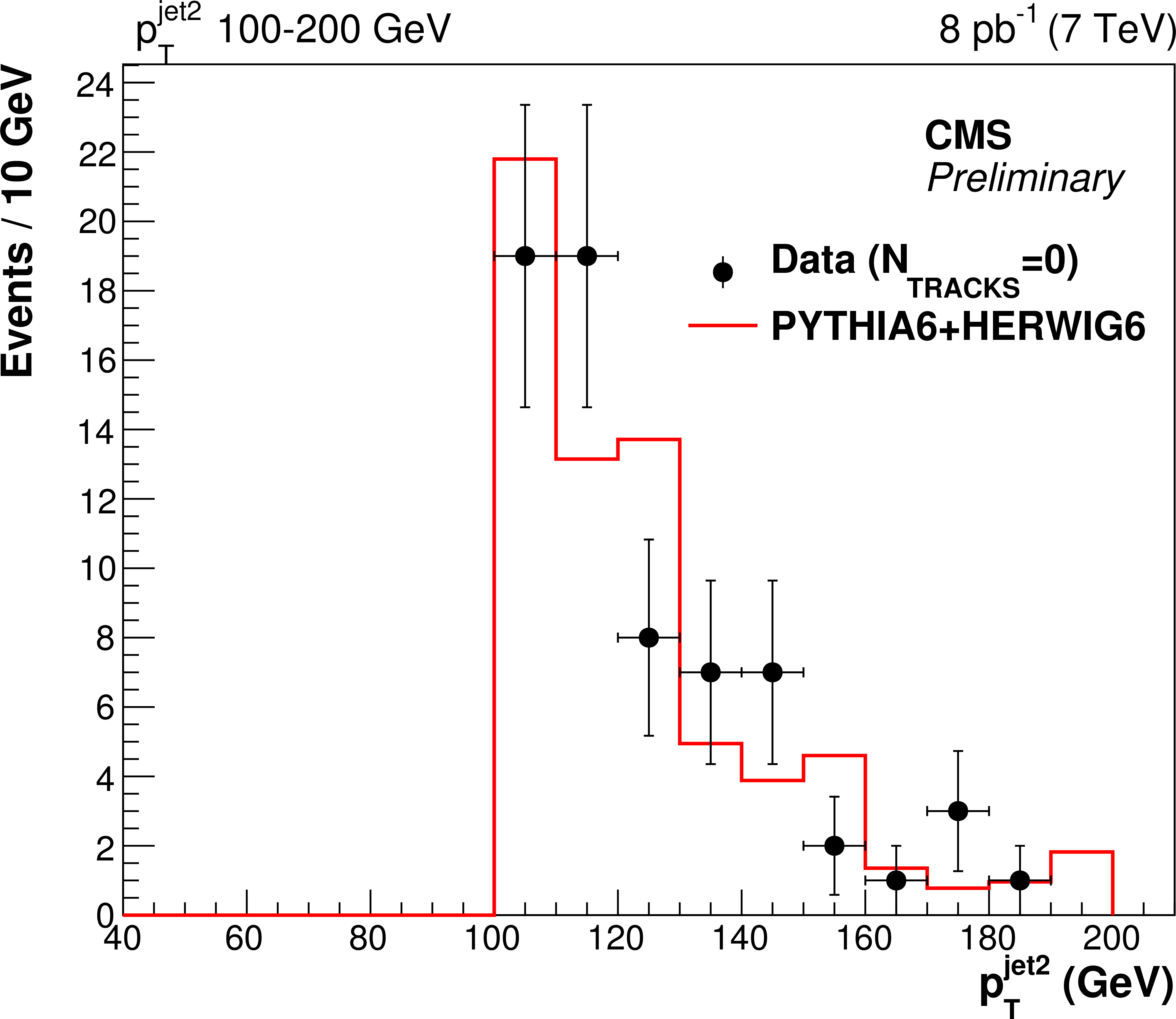
Figure 4-f:
Distributions of the leading jet (a,c,e) and the second-leading jet (b,d,f) $ {p_{\mathrm {T}}} $ for the three dijet samples with $40< {p_{\mathrm {T}}} ^\mathrm {jet2}<60$ GeV (a,b), $60< {p_{\mathrm {T}}} ^\mathrm {jet2}<100$ GeV (c,d), and $100< {p_{\mathrm {T}}} ^\mathrm {jet2}<200$ GeV (e,f) after all selections, for events with no tracks reconstructed in the rapidity gap region $|\eta |<1$, compared to MC predictions. The error bars indicate the statistical uncertainty. The normalization of the MC samples is obtained from a fit to the data from Fig. 3. |
png ; pdf |
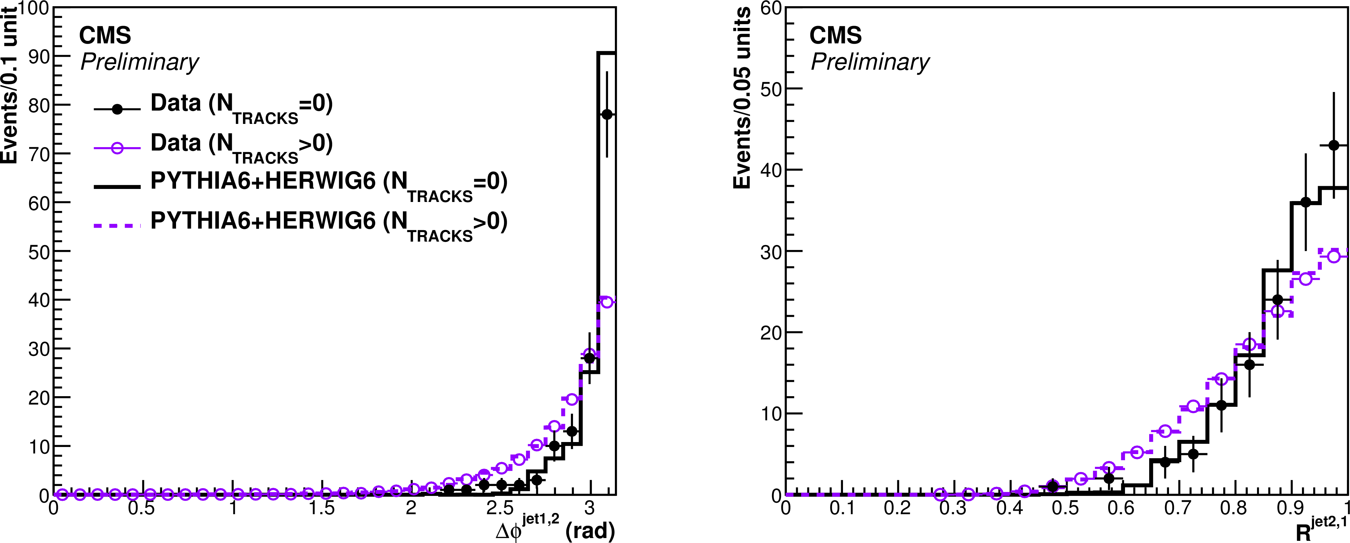
Figure 5:
Distributions of the azimuthal angle $ \Delta \phi^{\mathrm{jet1,2}} $ between the two leading jets (a) and the ratio $\rm {R}^{\rm{jet2,1}}$ of the second-leading jet $ {p_{\mathrm {T}}} $ to the leading jet $ {p_{\mathrm {T}}} $ (b) for events after all selections, with no tracks ($\rm {N}_{\rm {TRACKS}} = 0$, filled circles) or at least one track ($\rm {N}_{\rm {TRACKS}}> 0$, open circles) reconstructed in the $|\eta |<1$ region, compared with MC predictions. The distributions are summed over the three $p^\mathrm {jet2}_\mathrm {T}$ bins used in the analysis, and are normalized to the number of events in the data sample corresponding to $\rm {N}_{\rm {TRACKS}}= 0$. |
png ; pdf |
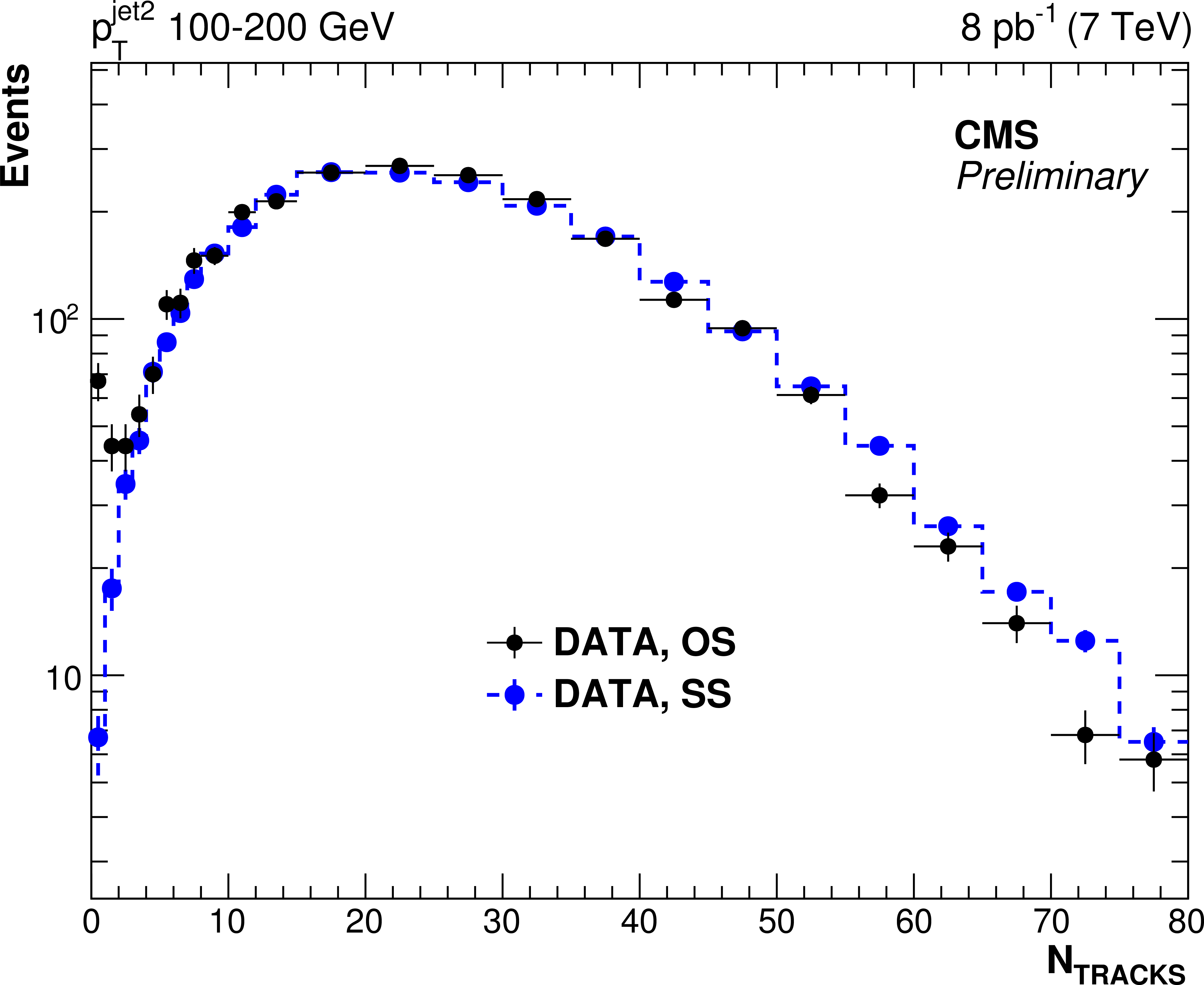
Figure 6-a:
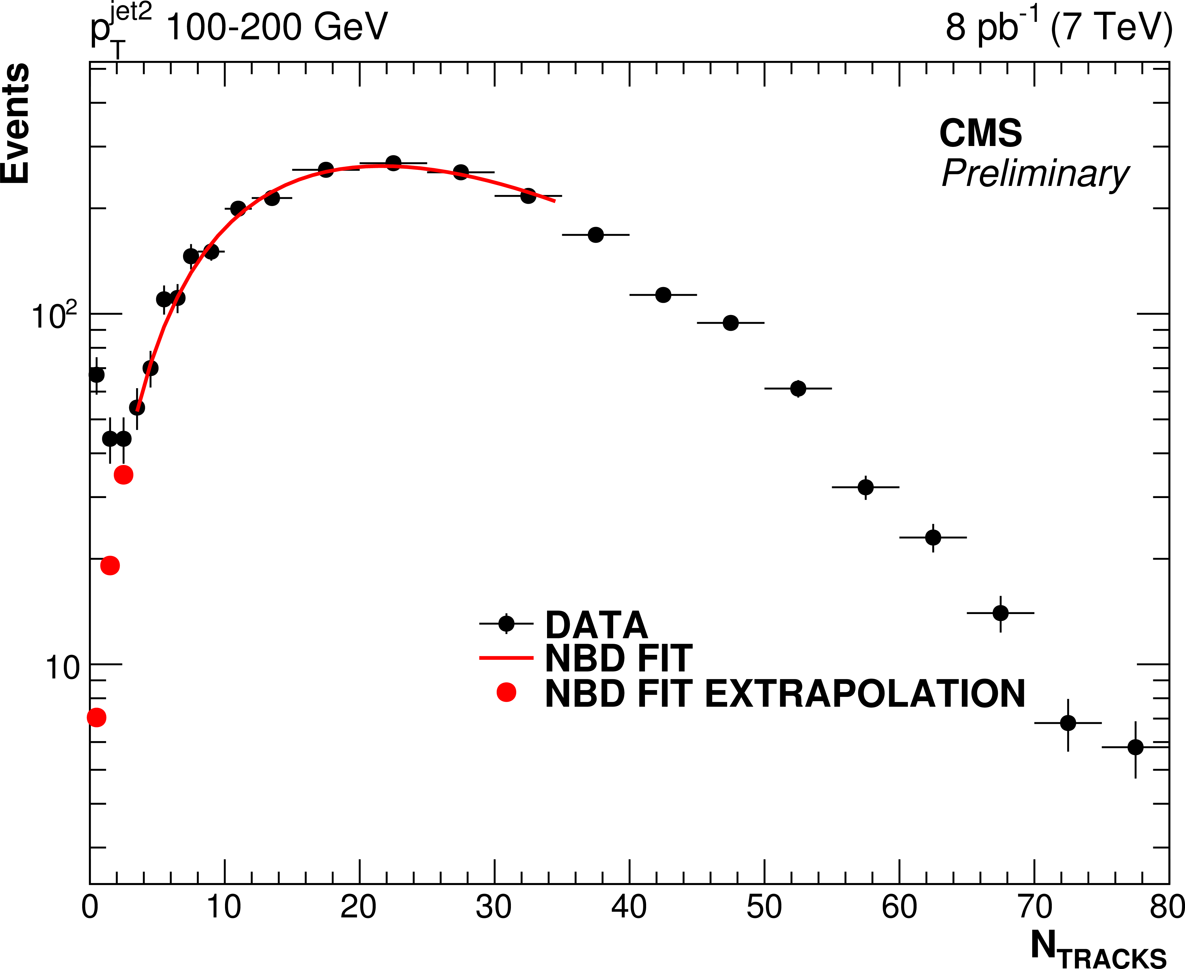
Charged multiplicity distribution in the highest $ {p_{\mathrm {T}}}^{\mathrm{jet2}}$ sample (100--200 GeV), shown together with the charged multiplicity distribution from the SS sample (a), and with the result of a fit with the Negative Binomial Distribution (NBD) function to the OS data (b). |
png ; pdf |
Figure 6-b:
Charged multiplicity distribution in the highest $ {p_{\mathrm {T}}}^{\mathrm{jet2}}$ sample (100--200 GeV), shown together with the charged multiplicity distribution from the SS sample (a), and with the result of a fit with the Negative Binomial Distribution (NBD) function to the OS data (b). |
png ; pdf |
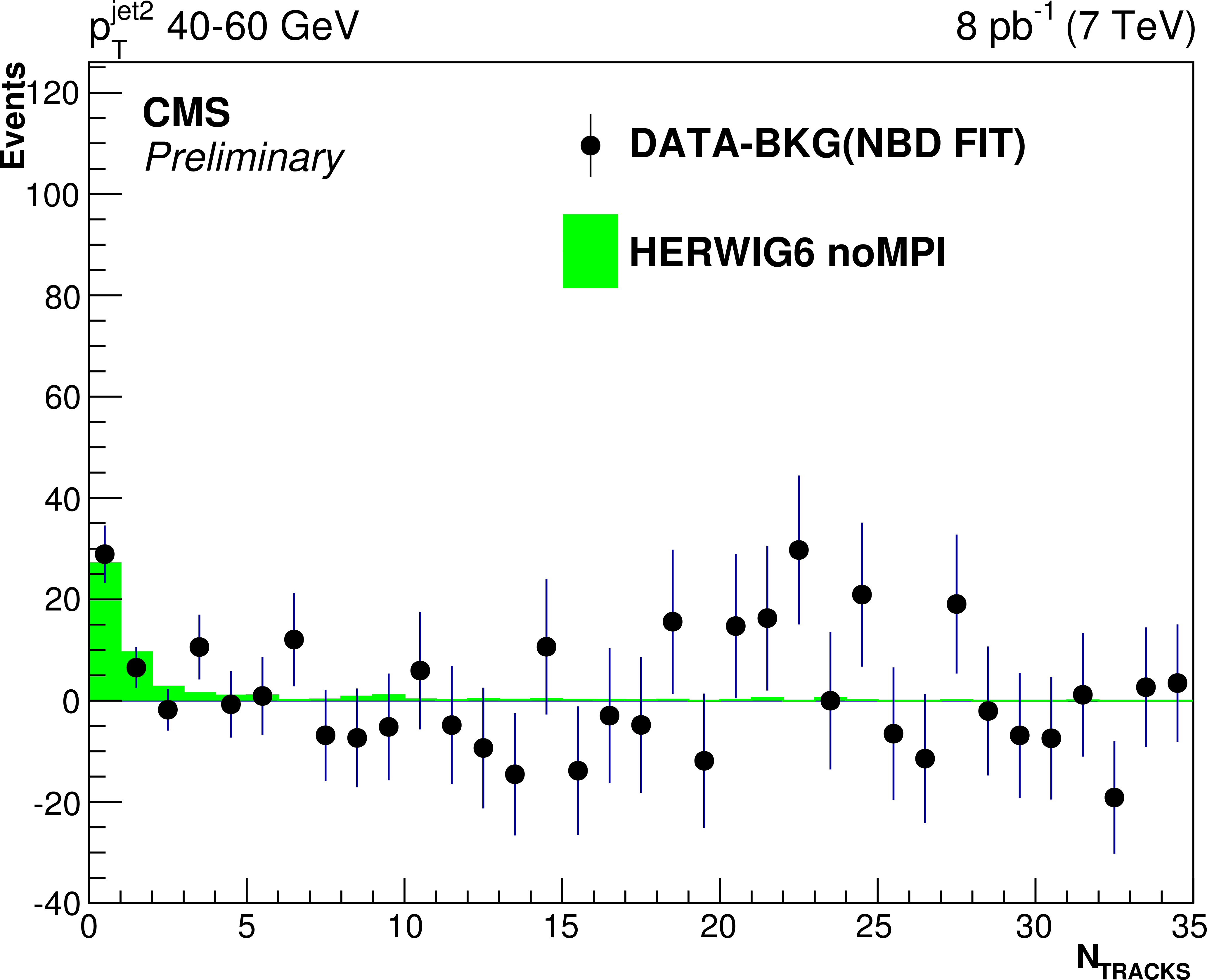
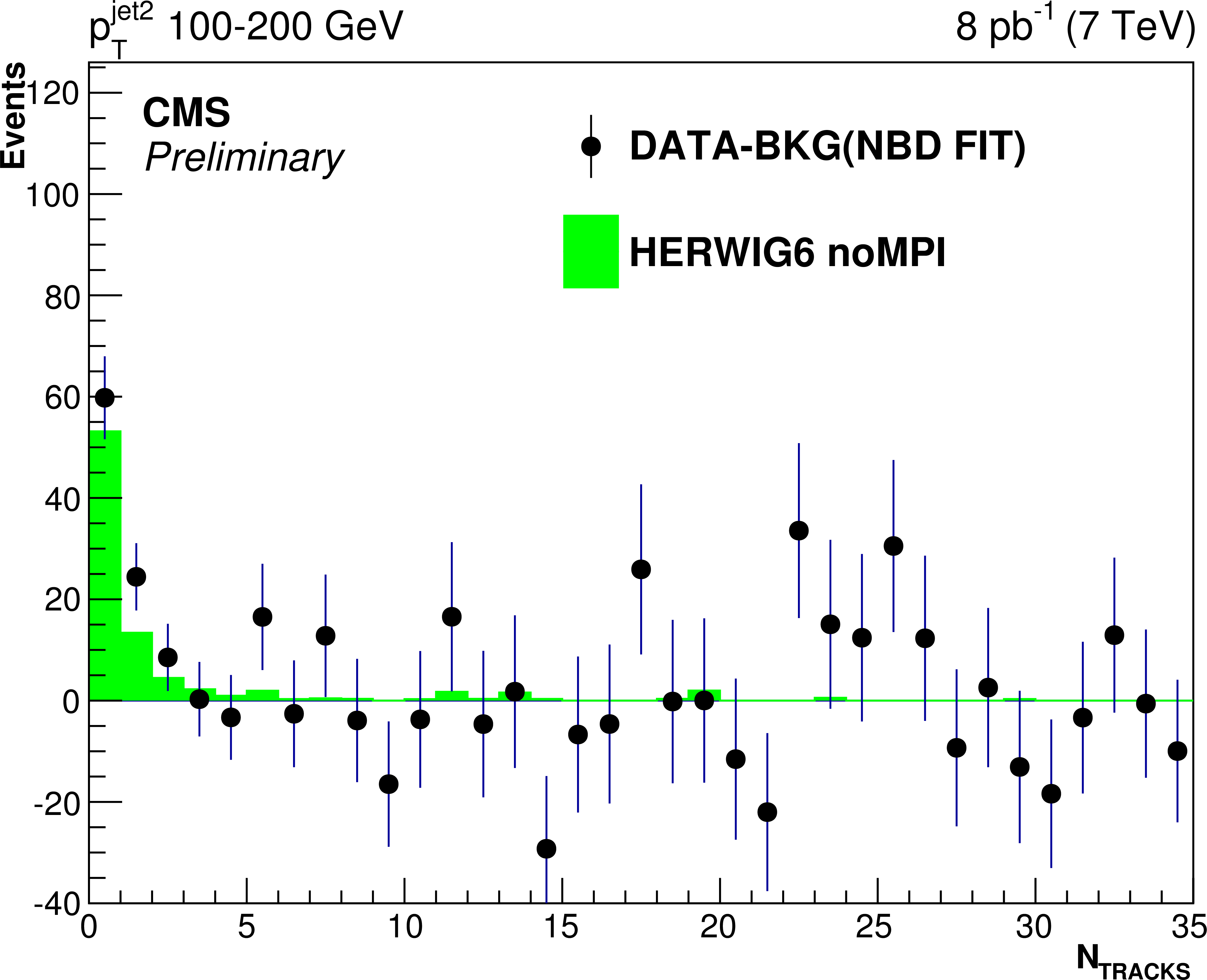
Figure 7-a:
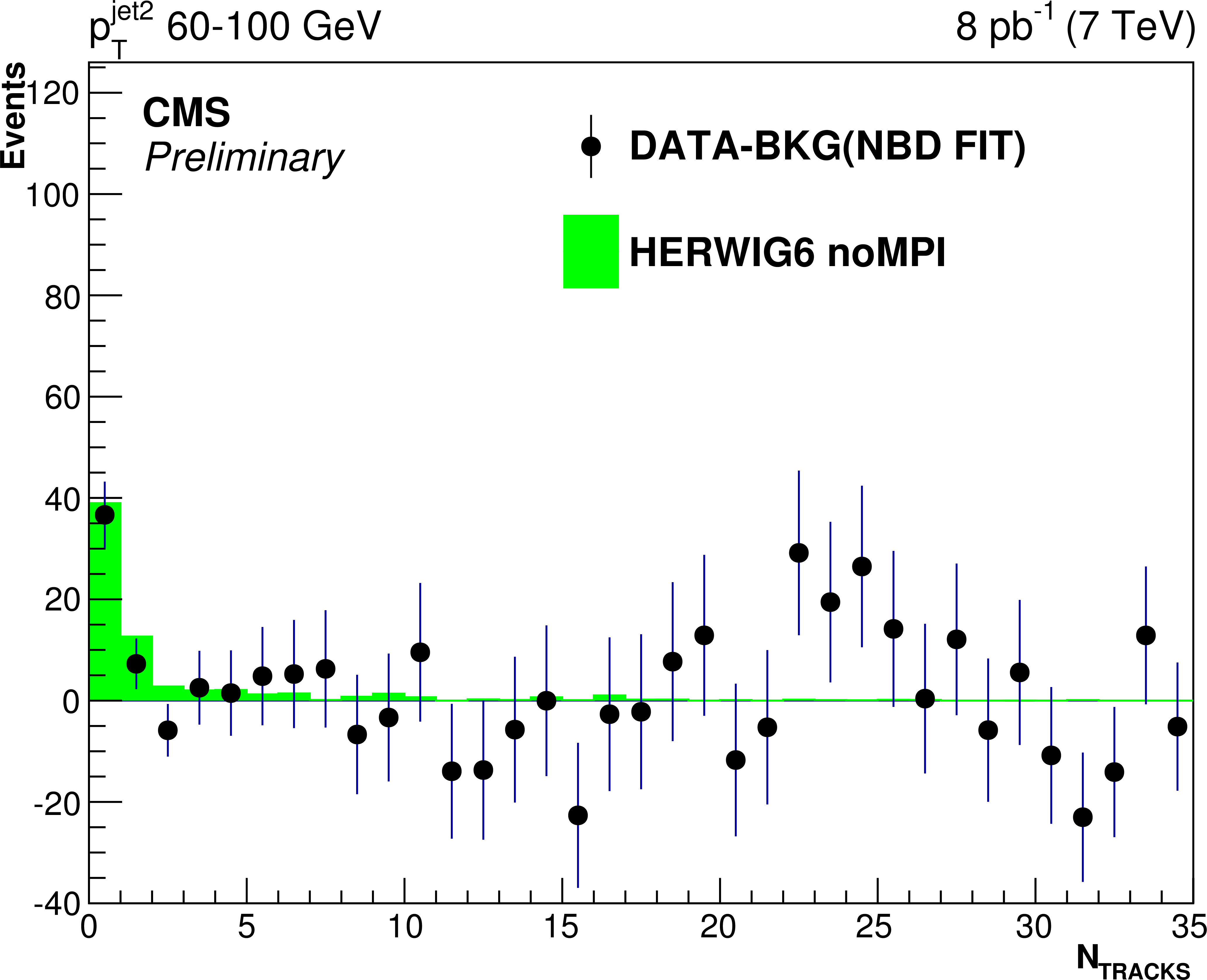
Background-subtracted charged multiplicity distributions in the three bins of $ {p_{\mathrm {T}}}^{\mathrm{jet2}}$, compared to the HERWIG6 predictions for events without an additional multiparton interaction (``noMPI''). The background is estimated from the NBD fit to the data in the $3 \le N_\mathrm {tracks} \le 35$ range, extrapolated to the lowest multiplicity bins. The normalization of the HERWIG6 MC is obtained from a fit to the data from Fig. 3. |
png ; pdf |
Figure 7-b:
Background-subtracted charged multiplicity distributions in the three bins of $ {p_{\mathrm {T}}}^{\mathrm{jet2}}$, compared to the HERWIG6 predictions for events without an additional multiparton interaction (``noMPI''). The background is estimated from the NBD fit to the data in the $3 \le N_\mathrm {tracks} \le 35$ range, extrapolated to the lowest multiplicity bins. The normalization of the HERWIG6 MC is obtained from a fit to the data from Fig. 3. |
png ; pdf |
Figure 7-c:
Background-subtracted charged multiplicity distributions in the three bins of $ {p_{\mathrm {T}}}^{\mathrm{jet2}}$, compared to the HERWIG6 predictions for events without an additional multiparton interaction (``noMPI''). The background is estimated from the NBD fit to the data in the $3 \le N_\mathrm {tracks} \le 35$ range, extrapolated to the lowest multiplicity bins. The normalization of the HERWIG6 MC is obtained from a fit to the data from Fig. 3. |
png ; pdf |
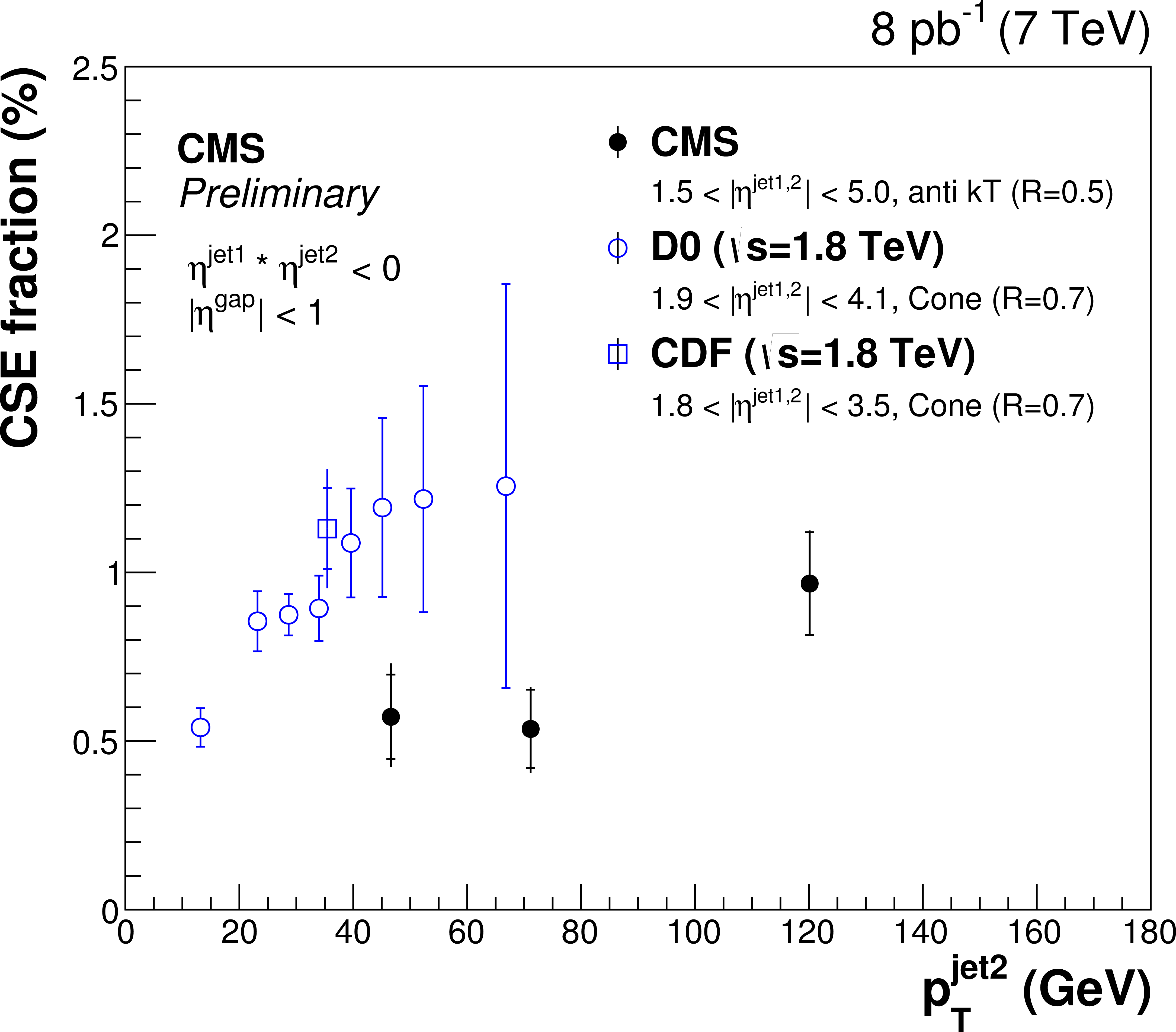
Figure 8:
The fraction $f_\mathrm {CSE}$ as a function of $ {p_{\mathrm {T}}}^{\mathrm{jet2}}$ as measured by CMS for $40< {p_{\mathrm {T}}}^{\mathrm{jet2}} <60$ GeV, $60< {p_{\mathrm {T}}}^{\mathrm{jet2}} <100$ GeV, and $100< {p_{\mathrm {T}}}^{\mathrm {jet2}} <200$ GeV at $\sqrt {s}=7$ TeV, and by D0 [14] and CDF [16] at $\sqrt {s}=1.8$ TeV. The details of the jet selections are given in the legend. The results are plotted at the mean value of $ {p_{\mathrm {T}}}^{\mathrm{jet2}}$ in the bin. The inner and outer error bars represent the statistical, and the statistical and systematic uncertainties added in quadrature, respectively. |
png ; pdf |
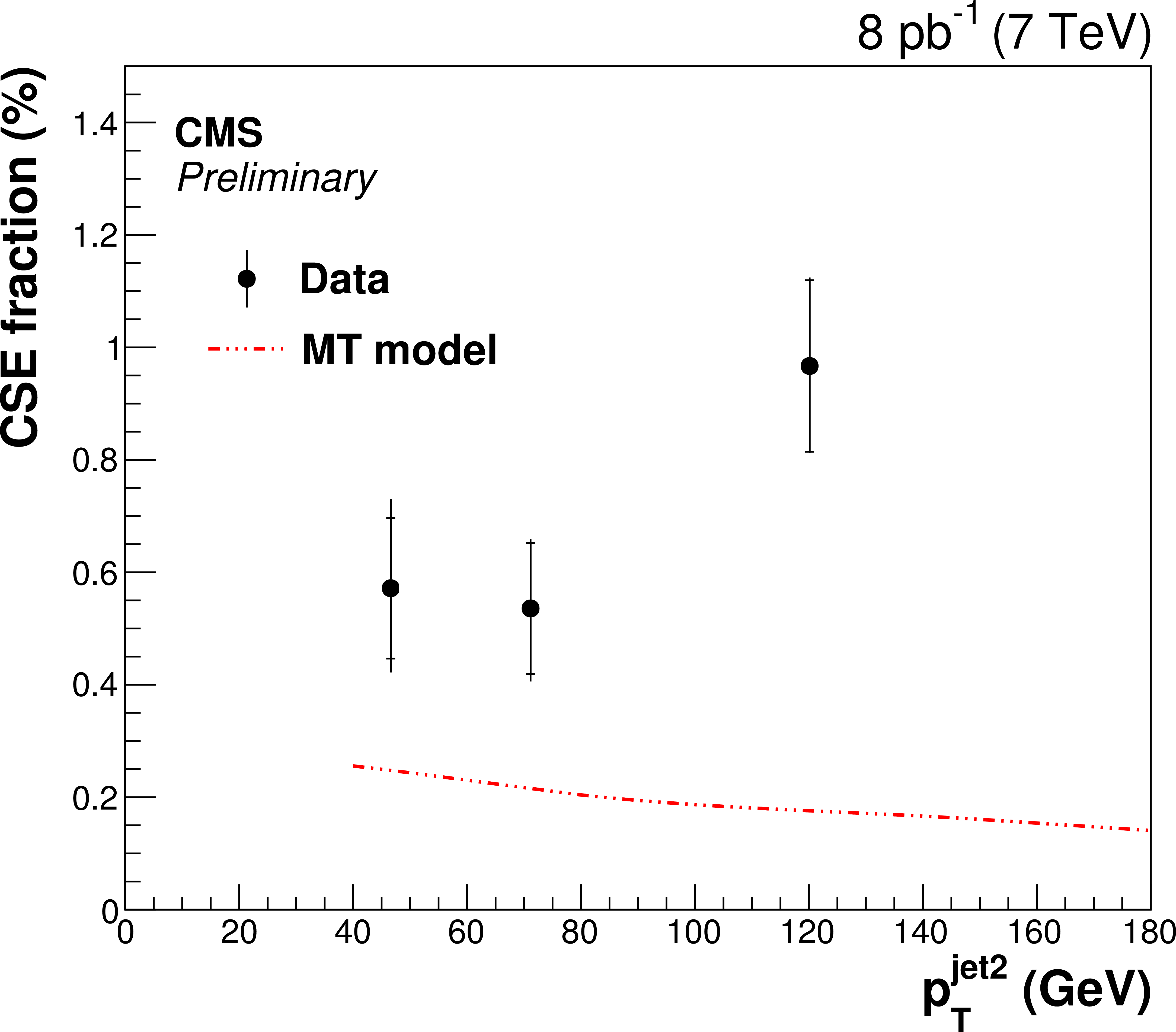
Figure 9:
The fraction $f_\mathrm {CSE}$ as a function of $ {p_{\mathrm {T}}}^{\mathrm{jet2}}$ measured for $40< {p_{\mathrm {T}}}^{\mathrm{jet2}} <60$ GeV, $60< {p_{\mathrm {T}}}^{\mathrm{jet2}} <100$ GeV, and $100< {p_{\mathrm {T}}}^{\mathrm{jet2}} <200$ GeV at $\sqrt {s}=7$ TeV, compared to the predictions of the MT model [9]. The results are plotted at the mean value of $ {p_{\mathrm {T}}}^{\mathrm{jet2}}$ in the bin. The inner and outer error bars represent the statistical, and the statistical and systematic uncertainties added in quadrature, respectively. |
png ; pdf |
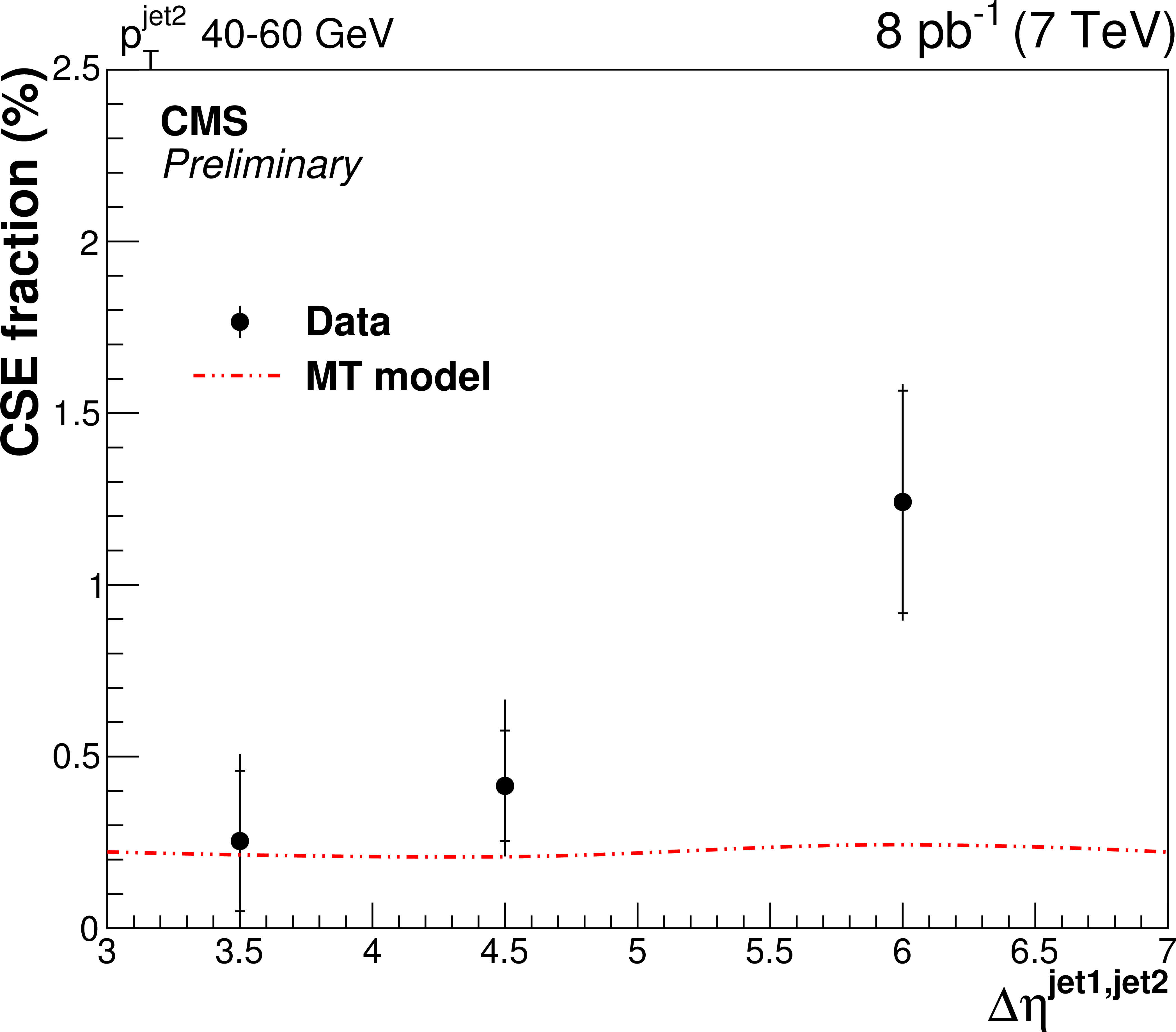
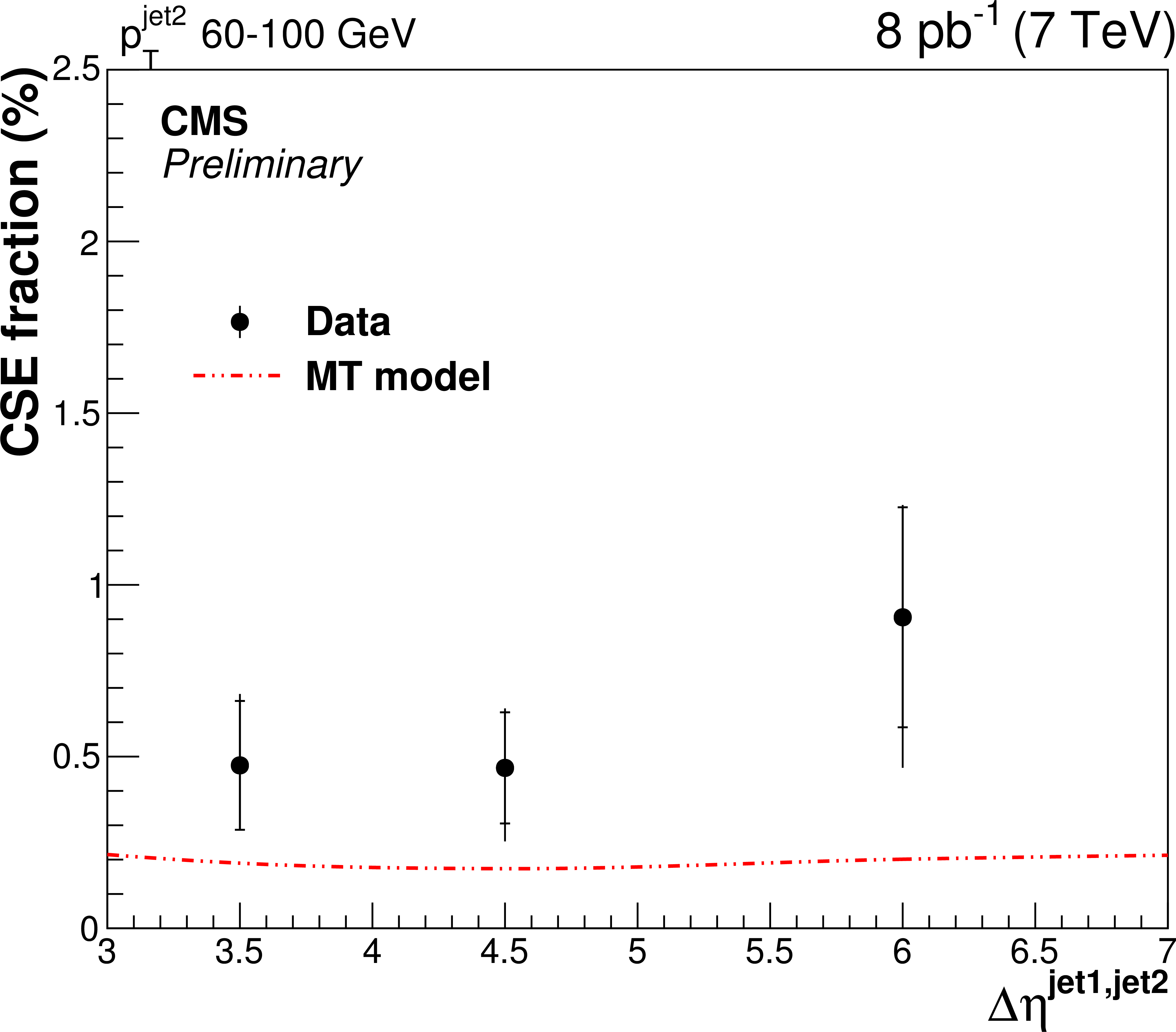
Figure 10-a:
The fraction $f_\mathrm {CSE}$ as a function of $\Delta \eta _\mathrm {jj}$ measured in the three bins of $p_{T}^\mathrm {jet2}$: 40-60 GeV, 60-100 GeV, and 100-200 GeV. The results are plotted at the center of the $\Delta \eta _\mathrm {jj}$ bin. Inner and outer error bars correspond to the statistical, and the statistical and systematic uncertainties added in quadrature, respectively. |
png ; pdf |
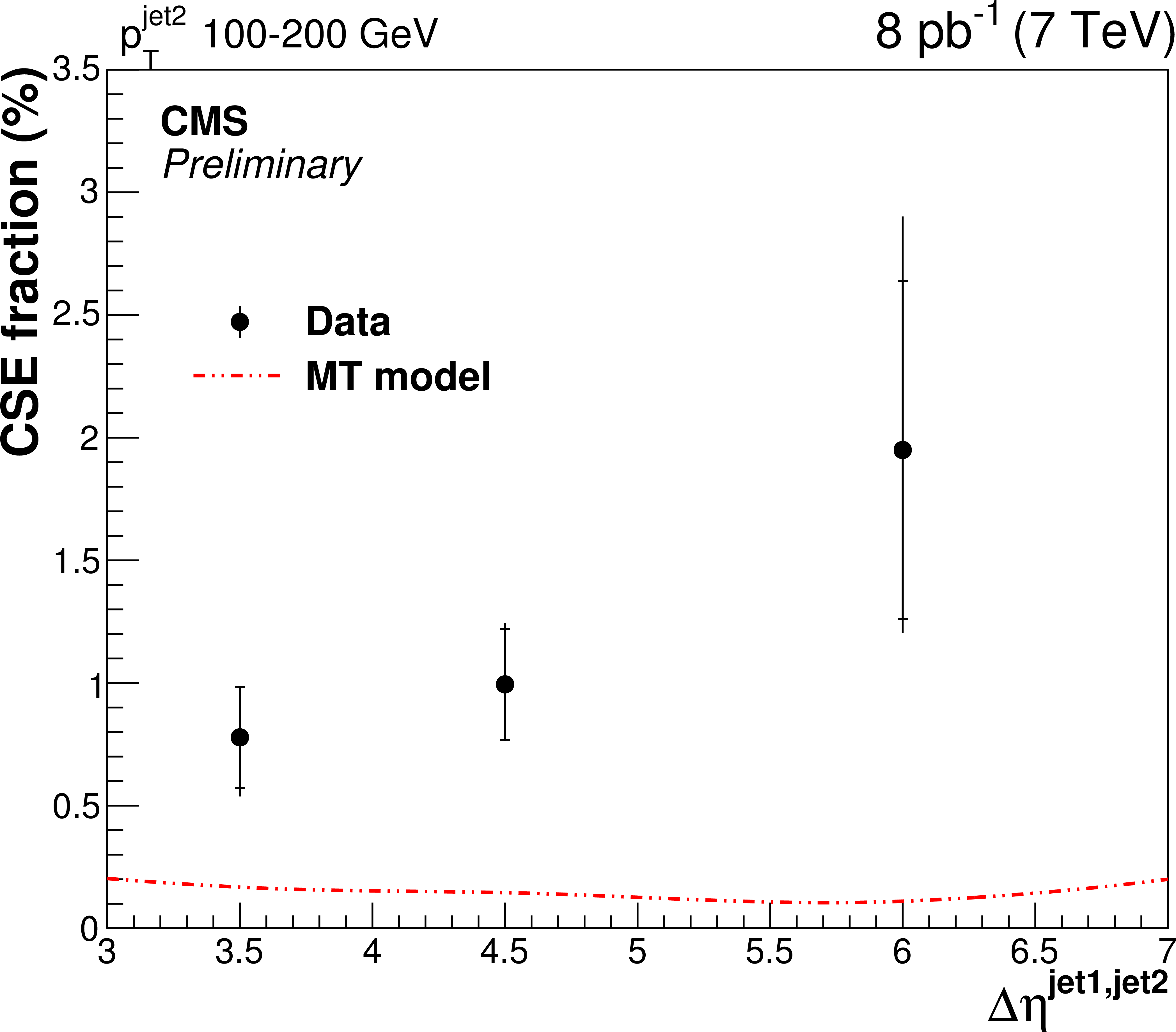
Figure 10-b:
The fraction $f_\mathrm {CSE}$ as a function of $\Delta \eta _\mathrm {jj}$ measured in the three bins of $p_{T}^\mathrm {jet2}$: 40-60 GeV, 60-100 GeV, and 100-200 GeV. The results are plotted at the center of the $\Delta \eta _\mathrm {jj}$ bin. Inner and outer error bars correspond to the statistical, and the statistical and systematic uncertainties added in quadrature, respectively. |
png ; pdf |
Figure 10-c:
The fraction $f_\mathrm {CSE}$ as a function of $\Delta \eta _\mathrm {jj}$ measured in the three bins of $p_{T}^\mathrm {jet2}$: 40-60 GeV, 60-100 GeV, and 100-200 GeV. The results are plotted at the center of the $\Delta \eta _\mathrm {jj}$ bin. Inner and outer error bars correspond to the statistical, and the statistical and systematic uncertainties added in quadrature, respectively. |
|
|
Compact Muon Solenoid LHC, CERN |
|

|

|

|

|

|