CMS-PAS-EXO-16-018

CMS-PAS-EXO-16-018
Search for new physics in high mass diphoton events in 3.3 fb $^{-1}$ of proton-proton collisions at $\sqrt{s}=$ 13 TeV and combined interpretation of searches at 8 TeV and 13 TeV
CMS Collaboration
March 2016

Abstract: We report on a search for new physics using high mass diphoton events. The search employs 3.3 fb $^{-1}$ of pp collision data collected by the CMS experiment in 2015 at a center-of-mass energy of 13 TeV. It is aimed at spin-0 and spin-2 resonances of mass between 500 and 4500 GeV and relative width up to $5.6 \times 10^{-2}$ . The results of the search are combined with those obtained by the CMS collaboration in similar searches at $\sqrt{s}=$ 8 TeV.
Links: CDS record (PDF) ; CADI line (restricted) ; These preliminary results are superseded in this paper, PRL 117 (2016) 051802. The superseded preliminary plots can be found here.

Figures
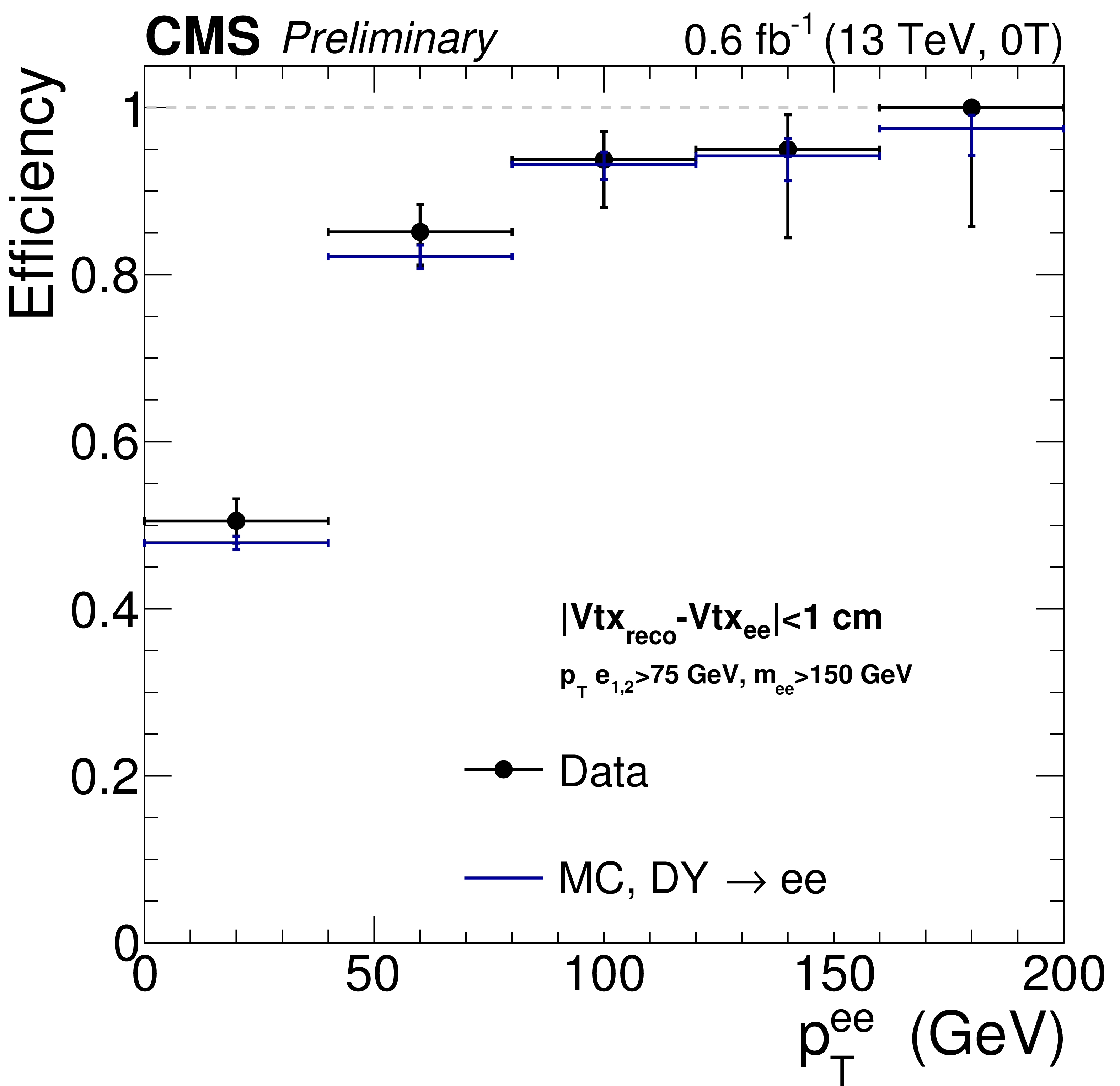
png pdf	Figure 1: Efficiency to find the correct vertex within 1cm for dielectron pairs with an invariant mass above 150 GeV in the B = 0 T dataset as a function of the dielectron transverse momentum. Data and simulated events are shown.
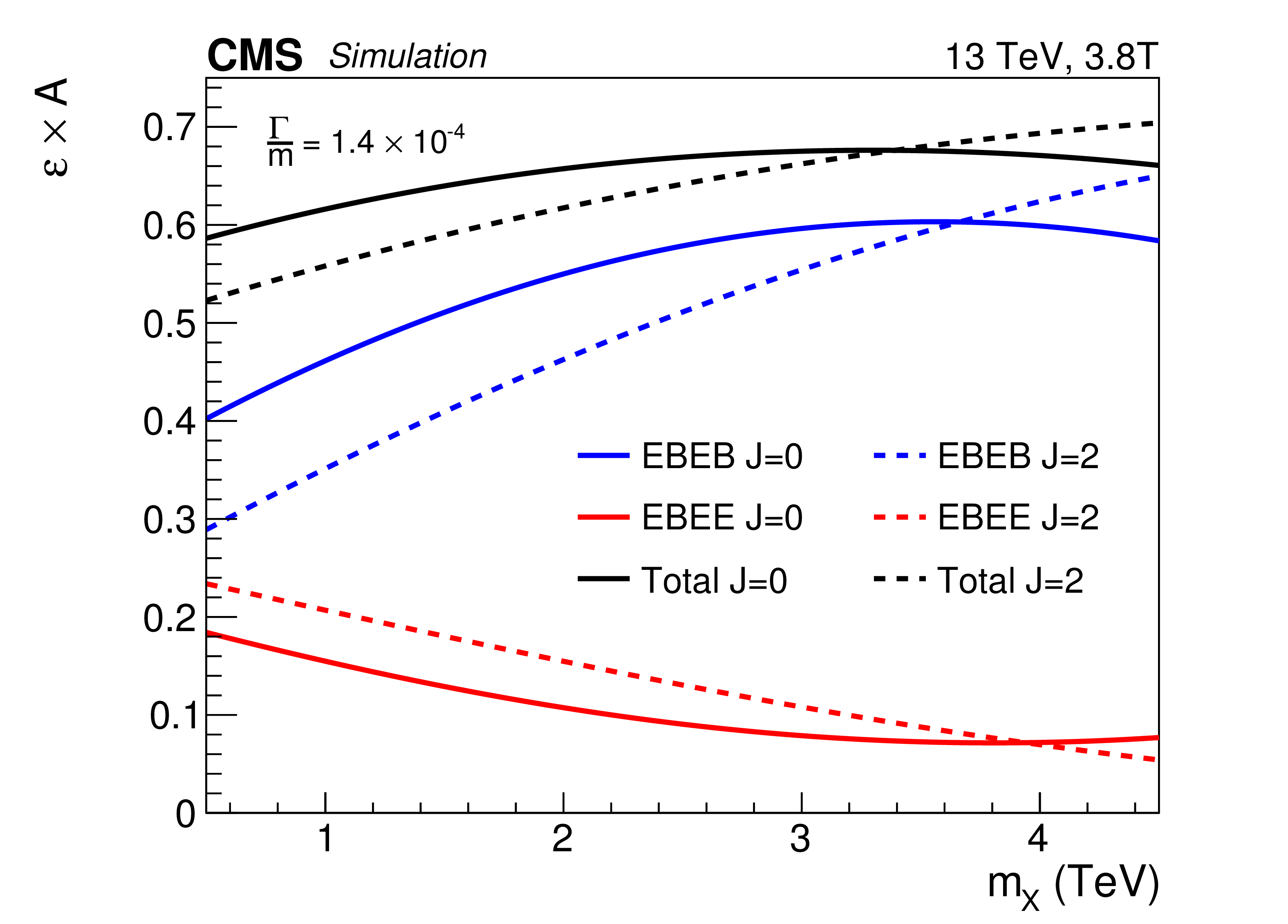
png pdf	Figure 2-a: Fraction of events selected by the analysis categories for 500 GeV $< {m} <$ 4.5 TeV and ${\Gamma / m} = 1.4\times 10^{-4}$ . Curves for both spin-0 and RS graviton resonances are shown, on the left for the B = 3.8 T sample and on the right for the B = 0 T one.
png pdf	Figure 2-b: Fraction of events selected by the analysis categories for 500 GeV $< {m} <$ 4.5 TeV and ${\Gamma / m} = 1.4\times 10^{-4}$ . Curves for both spin-0 and RS graviton resonances are shown, on the left for the B = 3.8 T sample and on the right for the B = 0 T one.
png	Figure 3-a: Comparison between the predicted and observed invariant mass distribution of electron pairs obtained after the application of energy scale and resolution corrections. Pairs of photon candidates satisfying the analysis identification criteria and compatible with electrons tracks are selected. Distributions are shown for events where both electrons are reconstructed in the barrel (a,c) and events where one electron is in an endcap (b.d). The (a,b) (c,d) row refers to the B = 3.8 T (B = 0 T) datasets. The simulation predictions are scaled to match the number of events observed in data.
png	Figure 3-b: Comparison between the predicted and observed invariant mass distribution of electron pairs obtained after the application of energy scale and resolution corrections. Pairs of photon candidates satisfying the analysis identification criteria and compatible with electrons tracks are selected. Distributions are shown for events where both electrons are reconstructed in the barrel (a,c) and events where one electron is in an endcap (b.d). The (a,b) (c,d) row refers to the B = 3.8 T (B = 0 T) datasets. The simulation predictions are scaled to match the number of events observed in data.
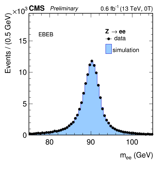
png	Figure 3-c: Comparison between the predicted and observed invariant mass distribution of electron pairs obtained after the application of energy scale and resolution corrections. Pairs of photon candidates satisfying the analysis identification criteria and compatible with electrons tracks are selected. Distributions are shown for events where both electrons are reconstructed in the barrel (a,c) and events where one electron is in an endcap (b.d). The (a,b) (c,d) row refers to the B = 3.8 T (B = 0 T) datasets. The simulation predictions are scaled to match the number of events observed in data.
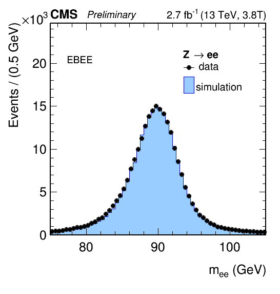
png	Figure 3-d: Comparison between the predicted and observed invariant mass distribution of electron pairs obtained after the application of energy scale and resolution corrections. Pairs of photon candidates satisfying the analysis identification criteria and compatible with electrons tracks are selected. Distributions are shown for events where both electrons are reconstructed in the barrel (a,c) and events where one electron is in an endcap (b.d). The (a,b) (c,d) row refers to the B = 3.8 T (B = 0 T) datasets. The simulation predictions are scaled to match the number of events observed in data.
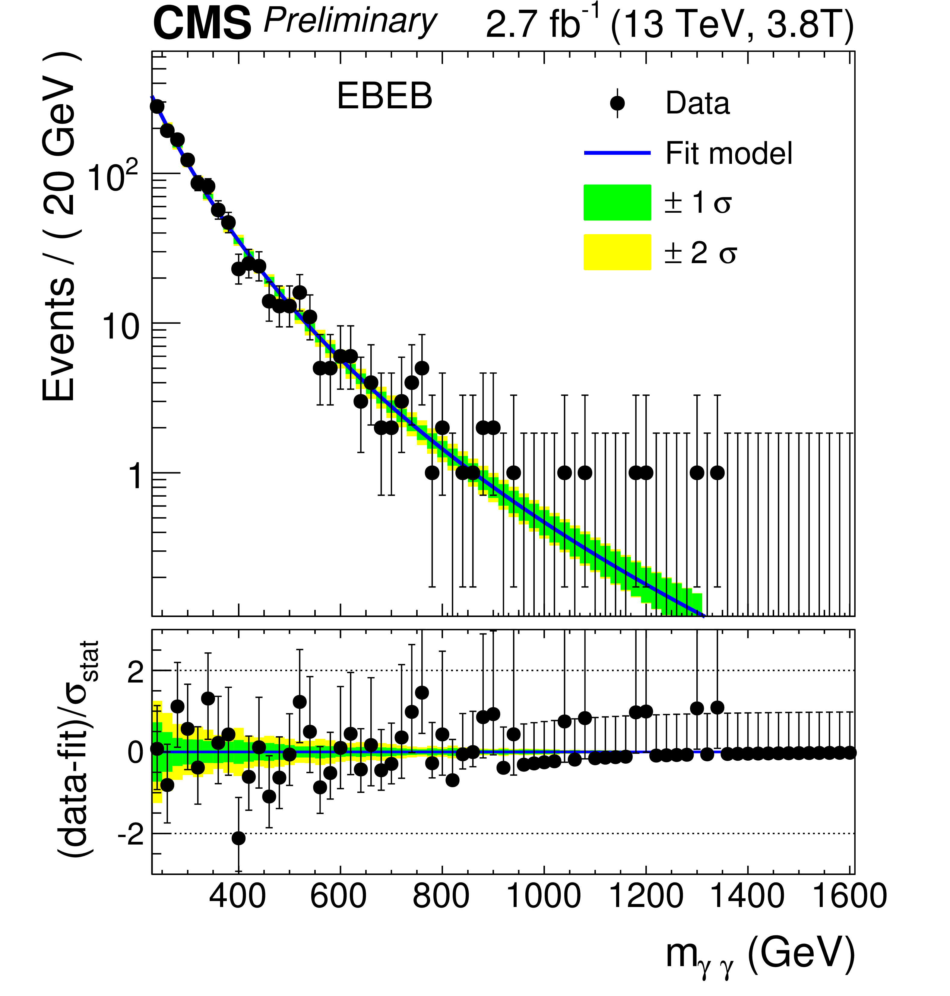
png pdf	Figure 4-a: Observed invariant mass spectra for the EBEB (a,c) and EBEE (b,d). (a,b) (c,d) row shows the B = 3.8 T (B = 0 T) dataset. The results of parametric fits to the data are also shown.
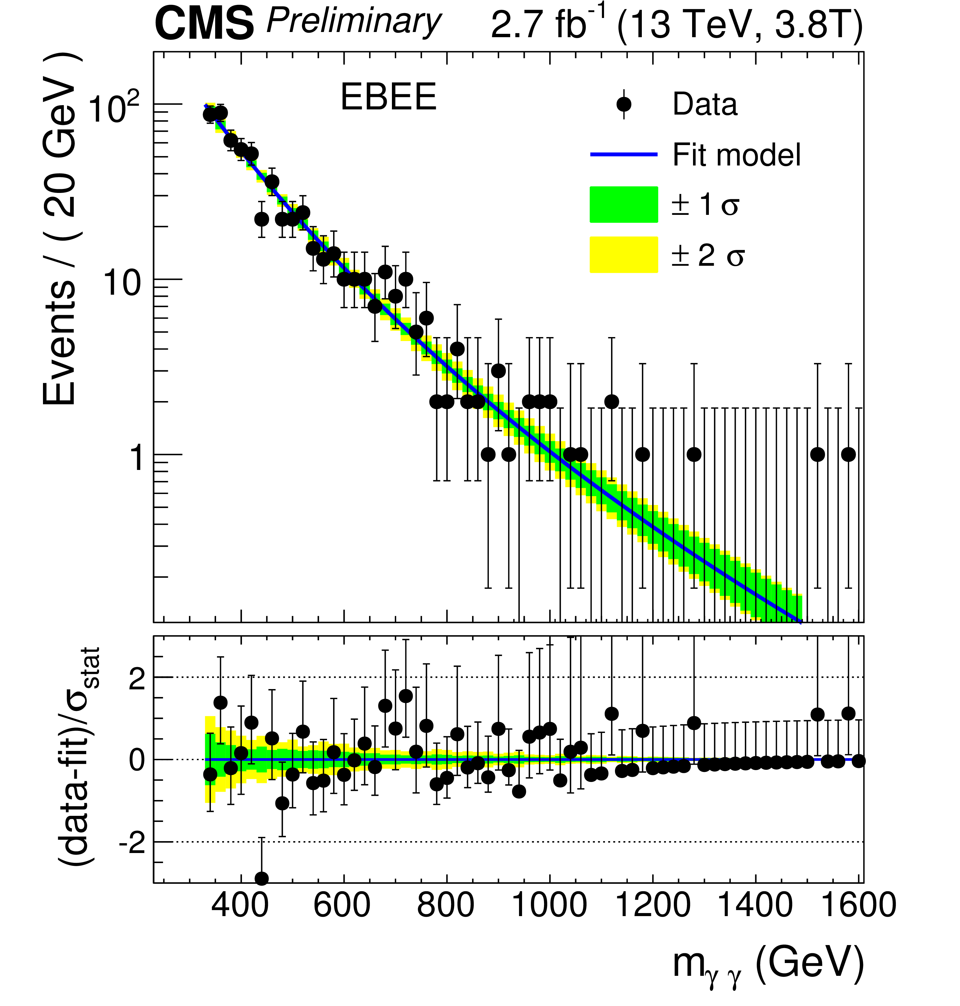
png pdf	Figure 4-b: Observed invariant mass spectra for the EBEB (a,c) and EBEE (b,d). (a,b) (c,d) row shows the B = 3.8 T (B = 0 T) dataset. The results of parametric fits to the data are also shown.
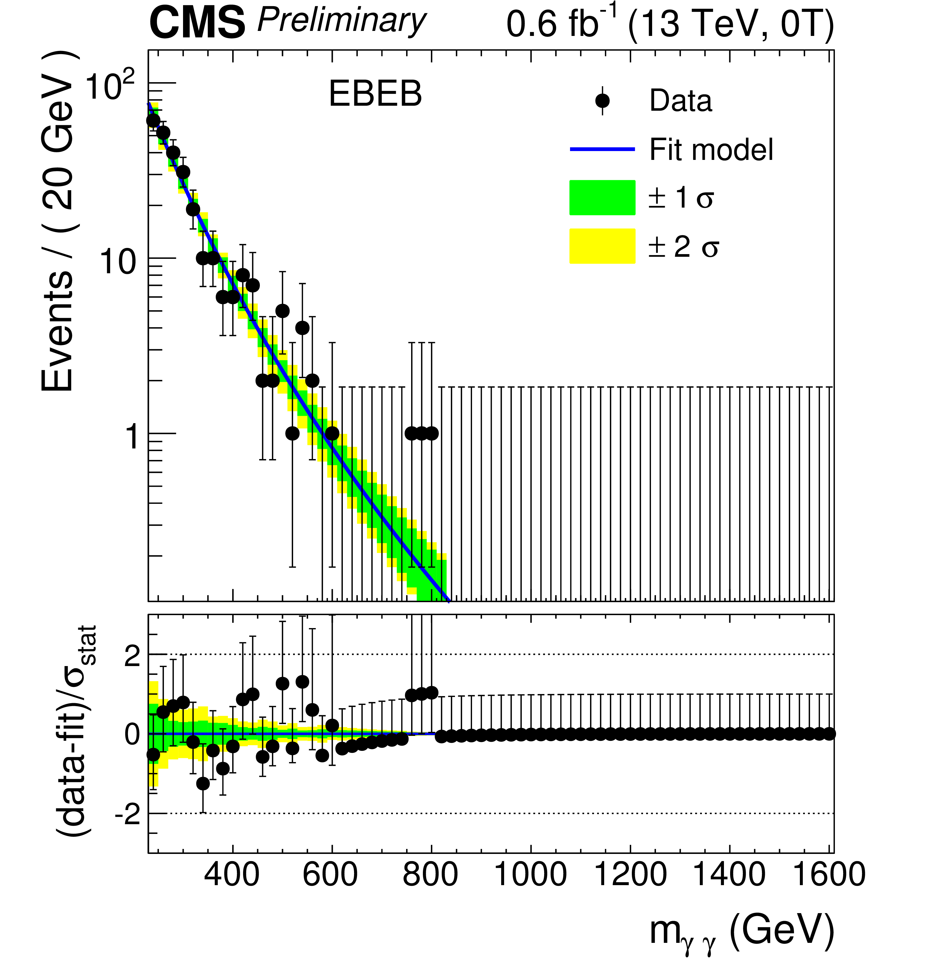
png pdf	Figure 4-c: Observed invariant mass spectra for the EBEB (a,c) and EBEE (b,d). (a,b) (c,d) row shows the B = 3.8 T (B = 0 T) dataset. The results of parametric fits to the data are also shown.
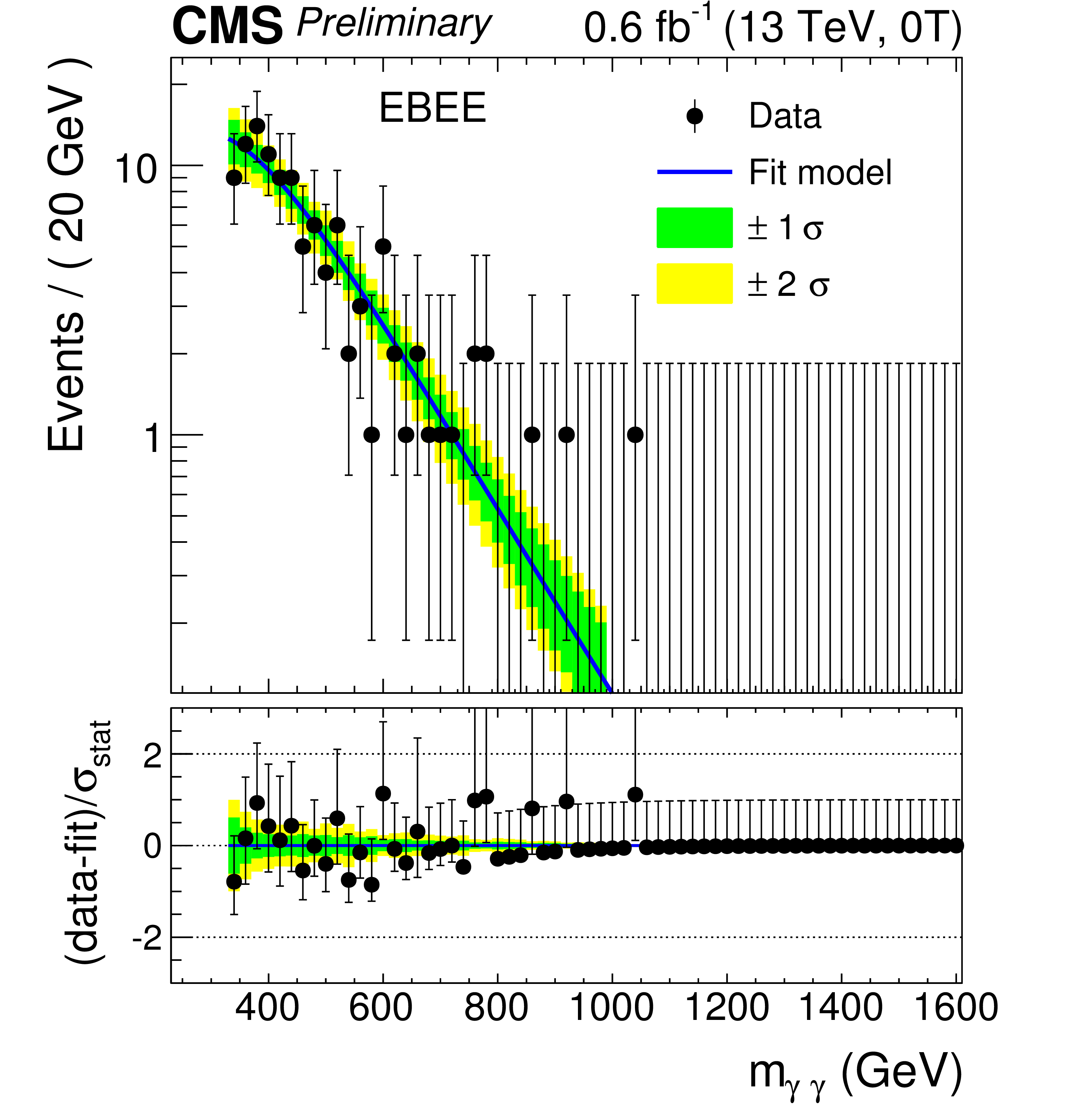
png pdf	Figure 4-d: Observed invariant mass spectra for the EBEB (a,c) and EBEE (b,d). (a,b) (c,d) row shows the B = 3.8 T (B = 0 T) dataset. The results of parametric fits to the data are also shown.
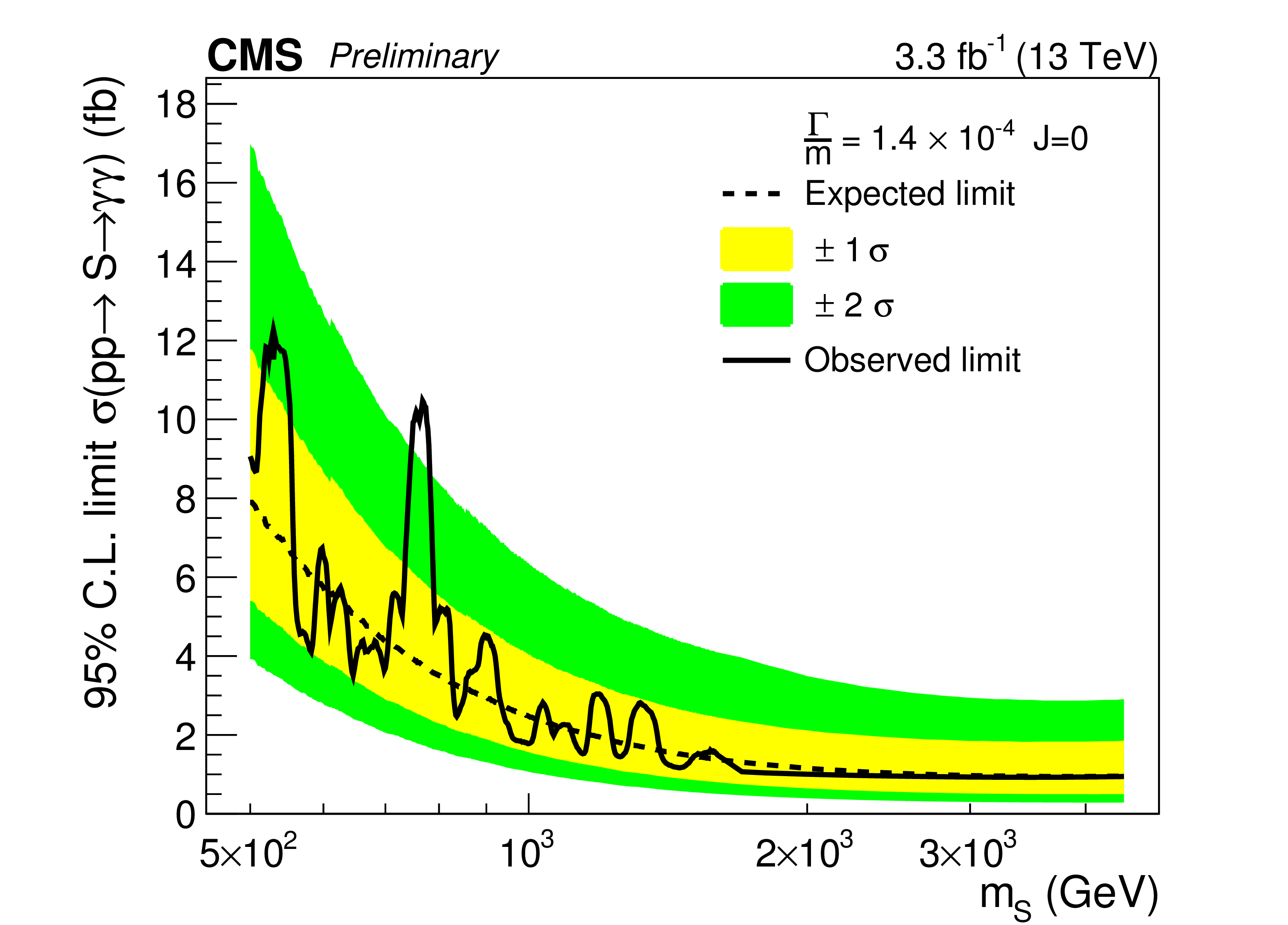
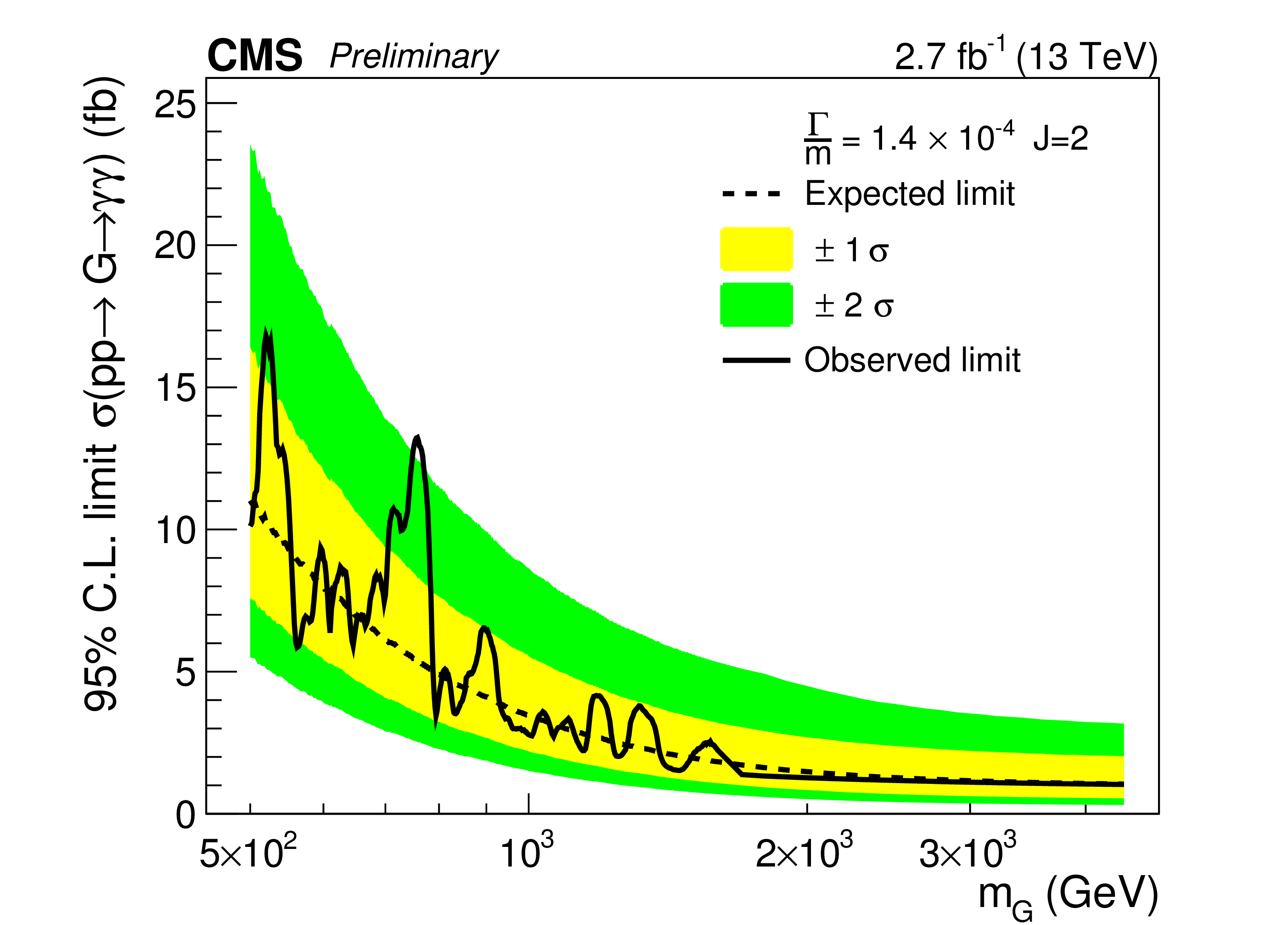
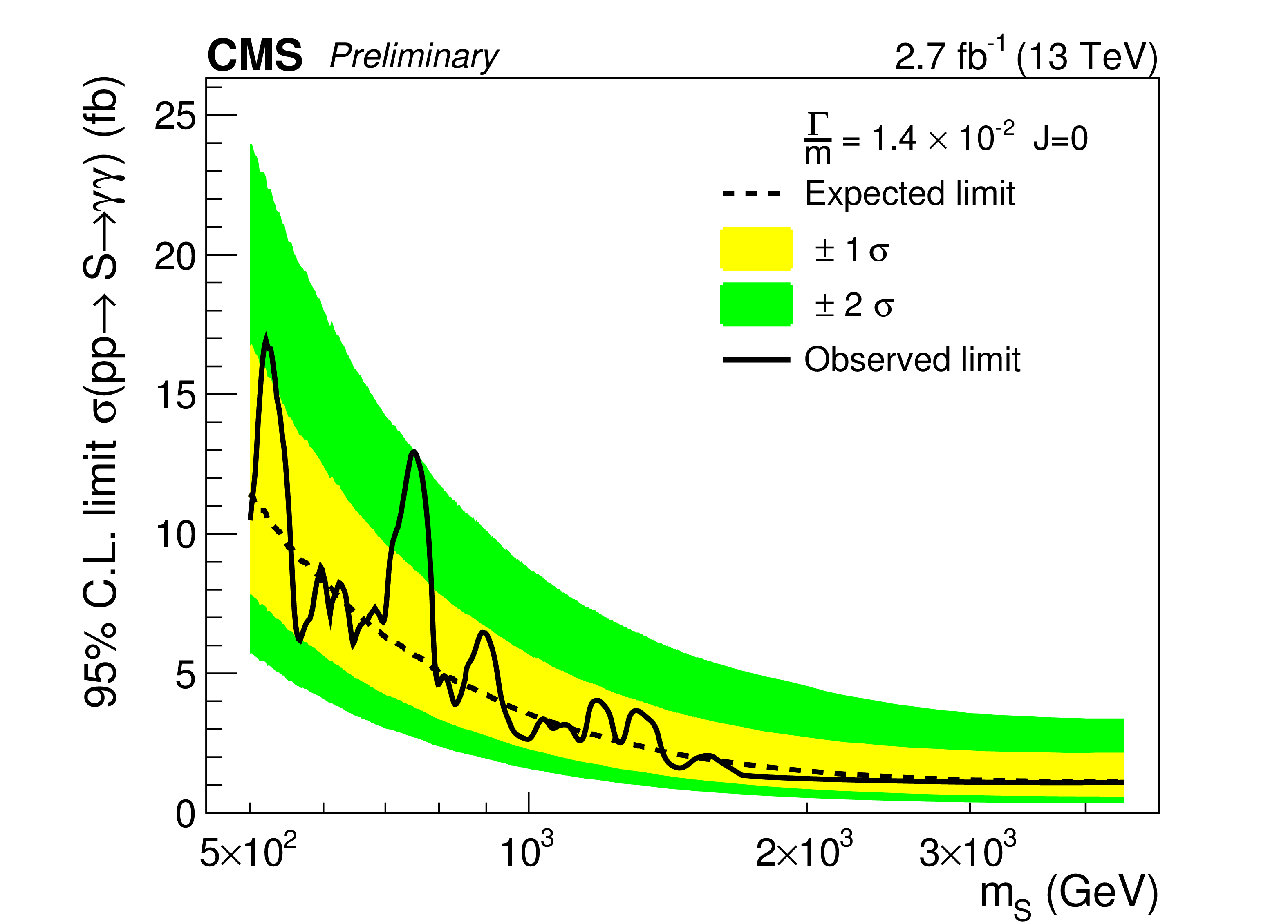
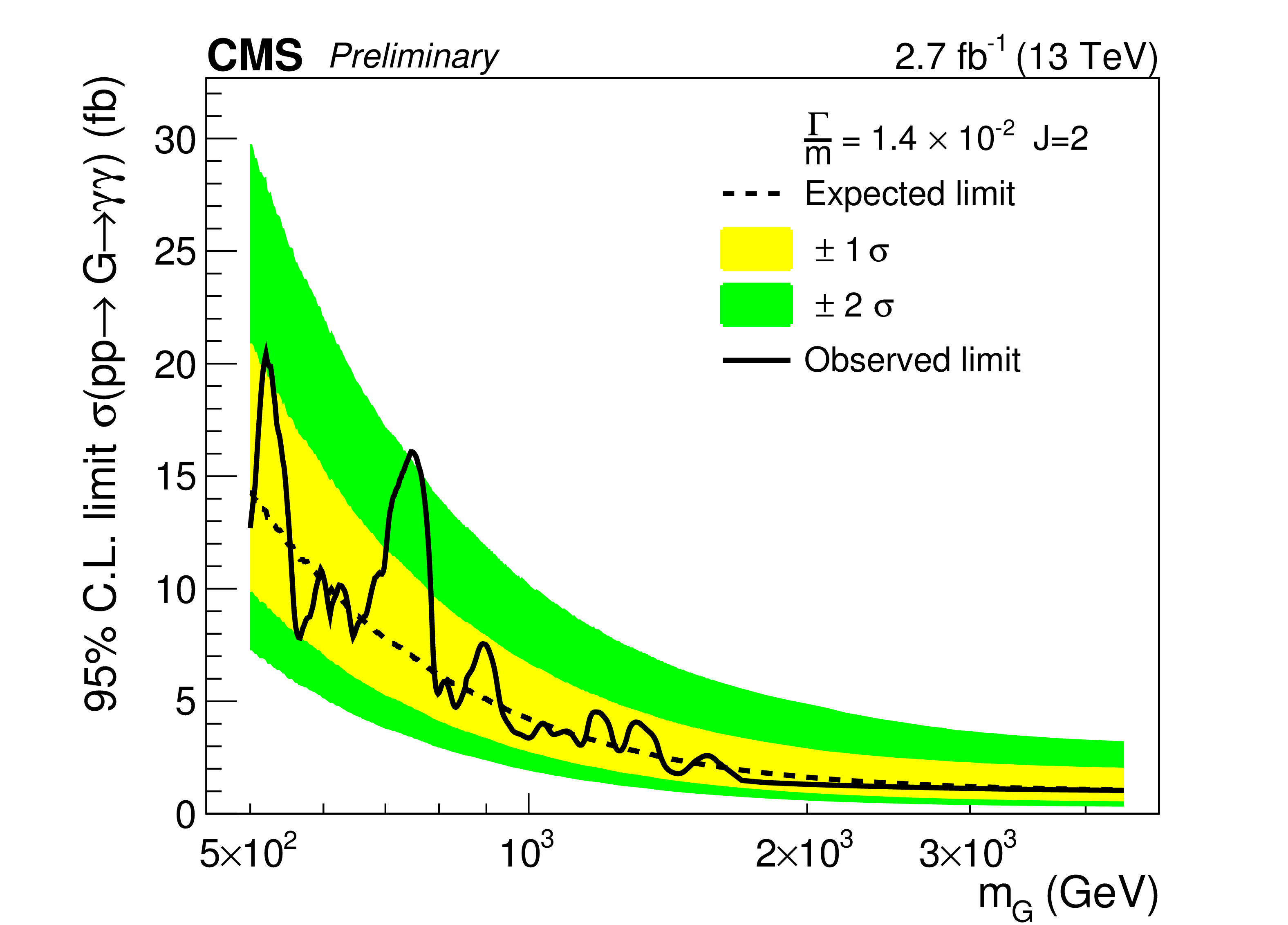
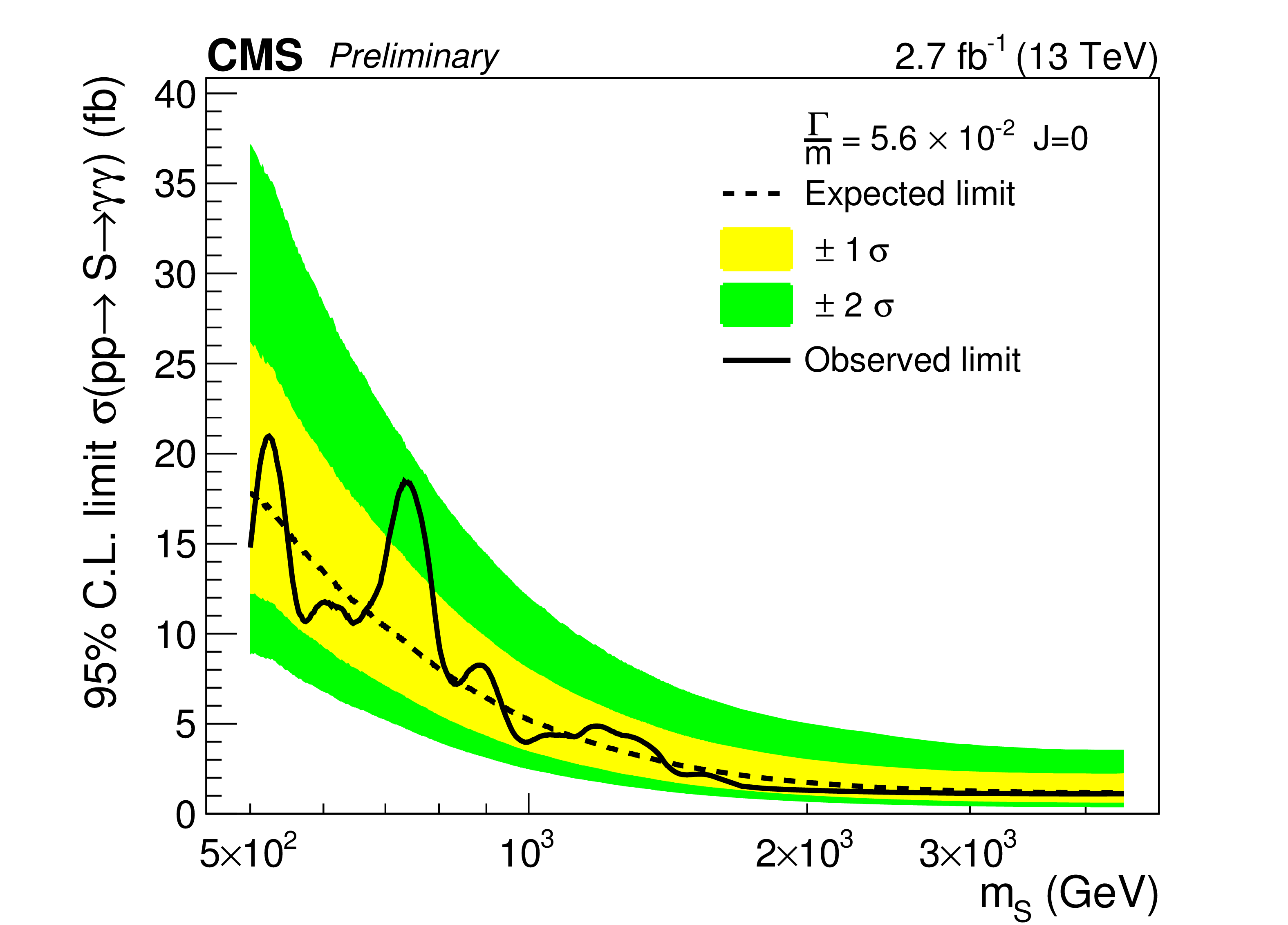
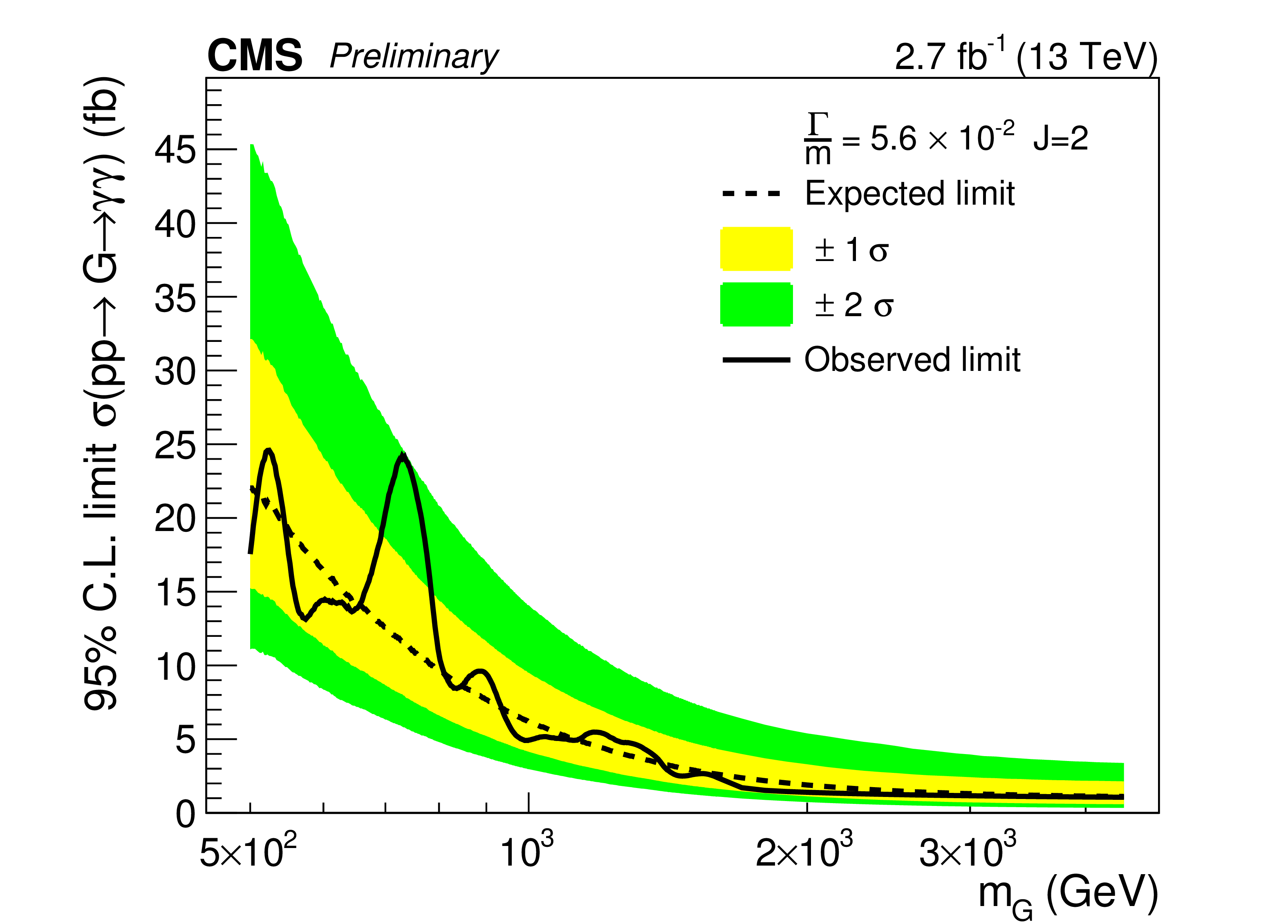
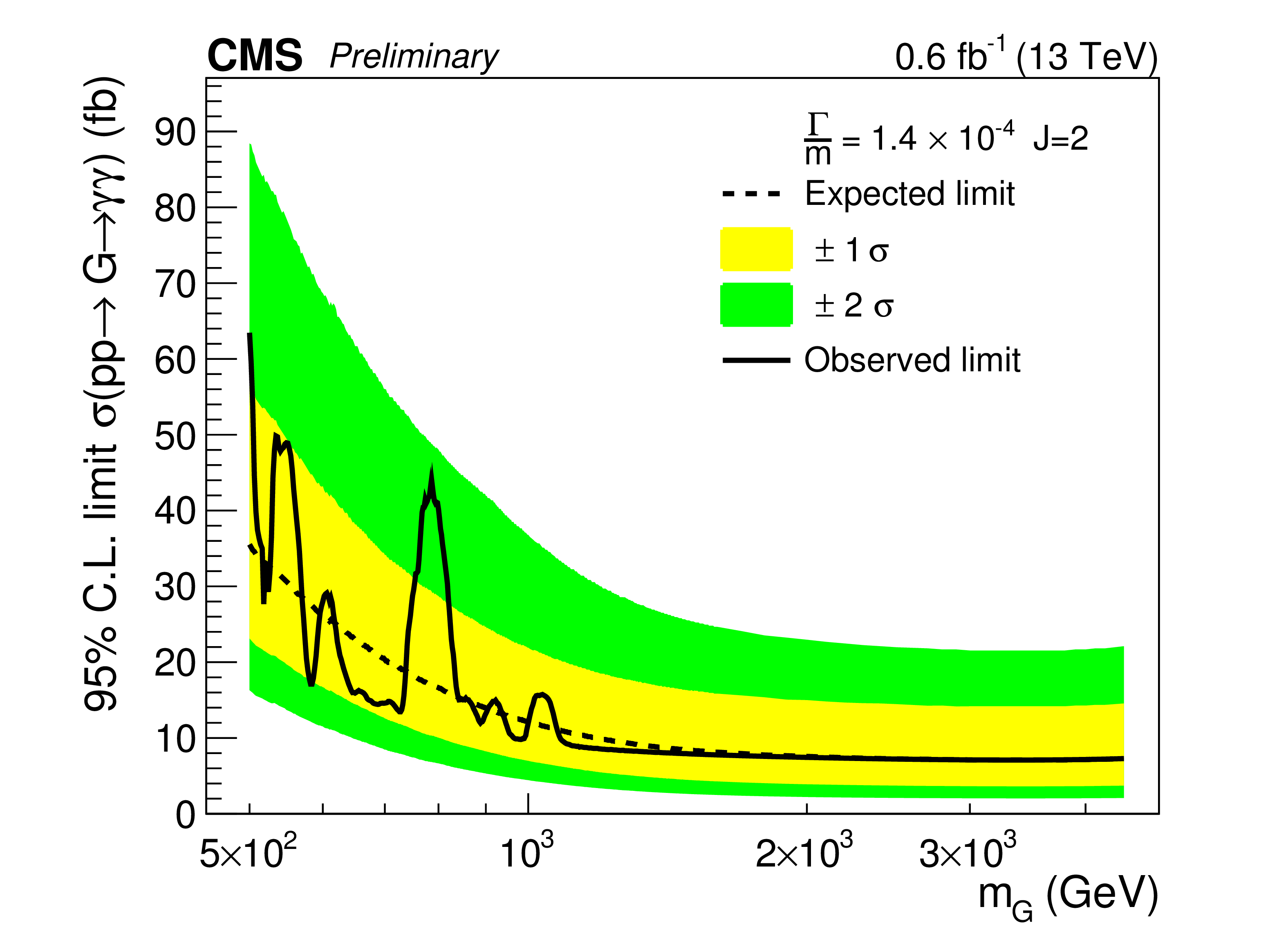
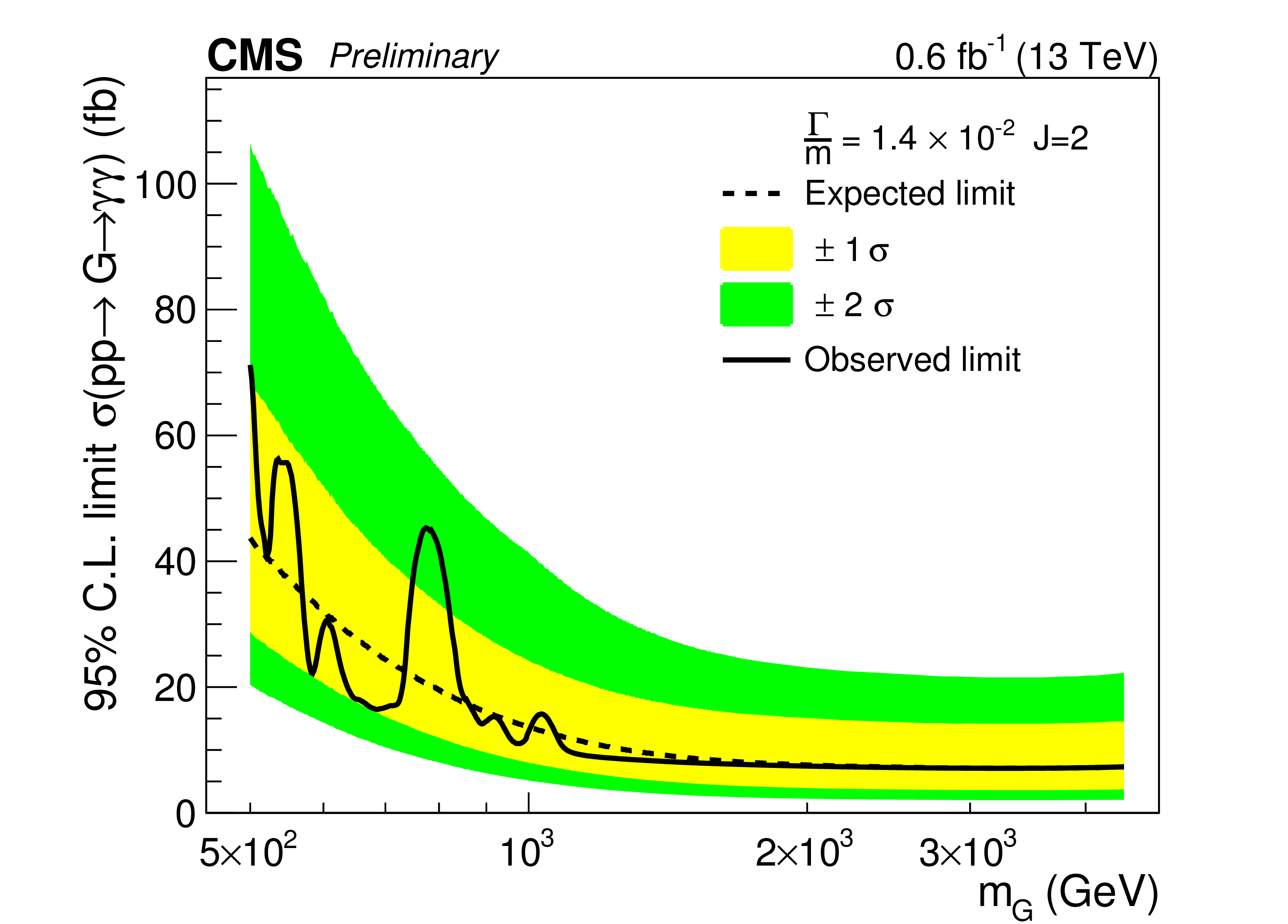
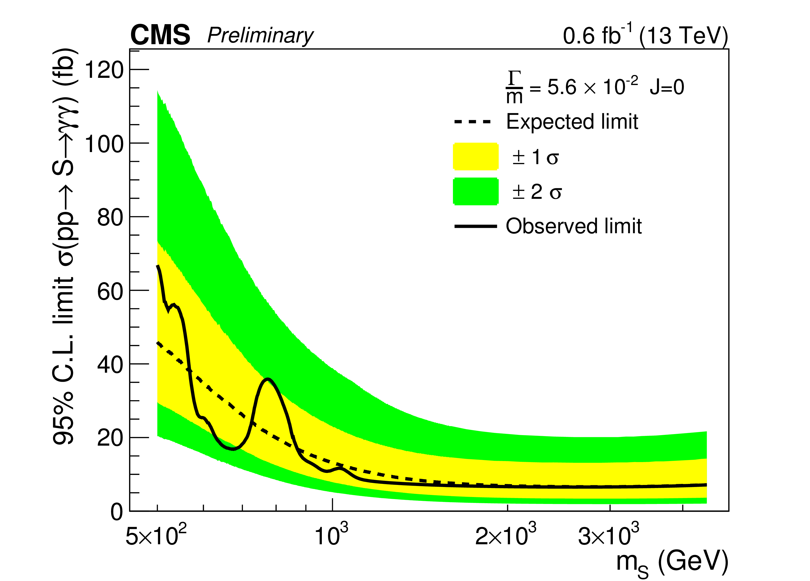
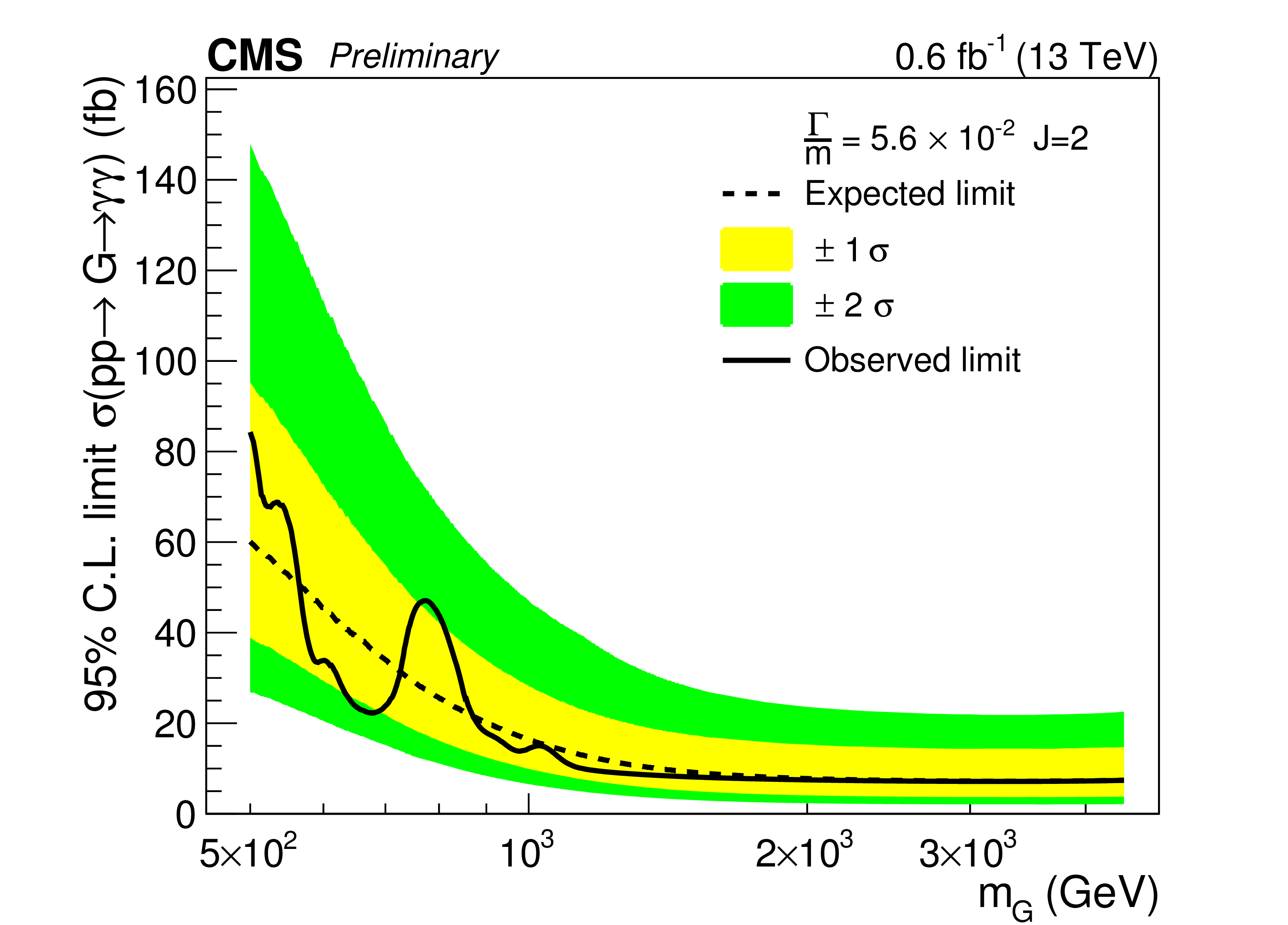
png pdf	Figure 5-a: Expected and observed 95% C.L. exclusion limits for different signal hypotheses. The range 500 GeV $< m <$ 4.5 TeV is shown for ${\Gamma / m} = 1.4\times 10^{-4}$ , $1.4\times 10^{-2}$ , $5.6\times 10^{-2}$ . The (a,c) (b,d) column corresponds to the scalar (RS graviton) signals.
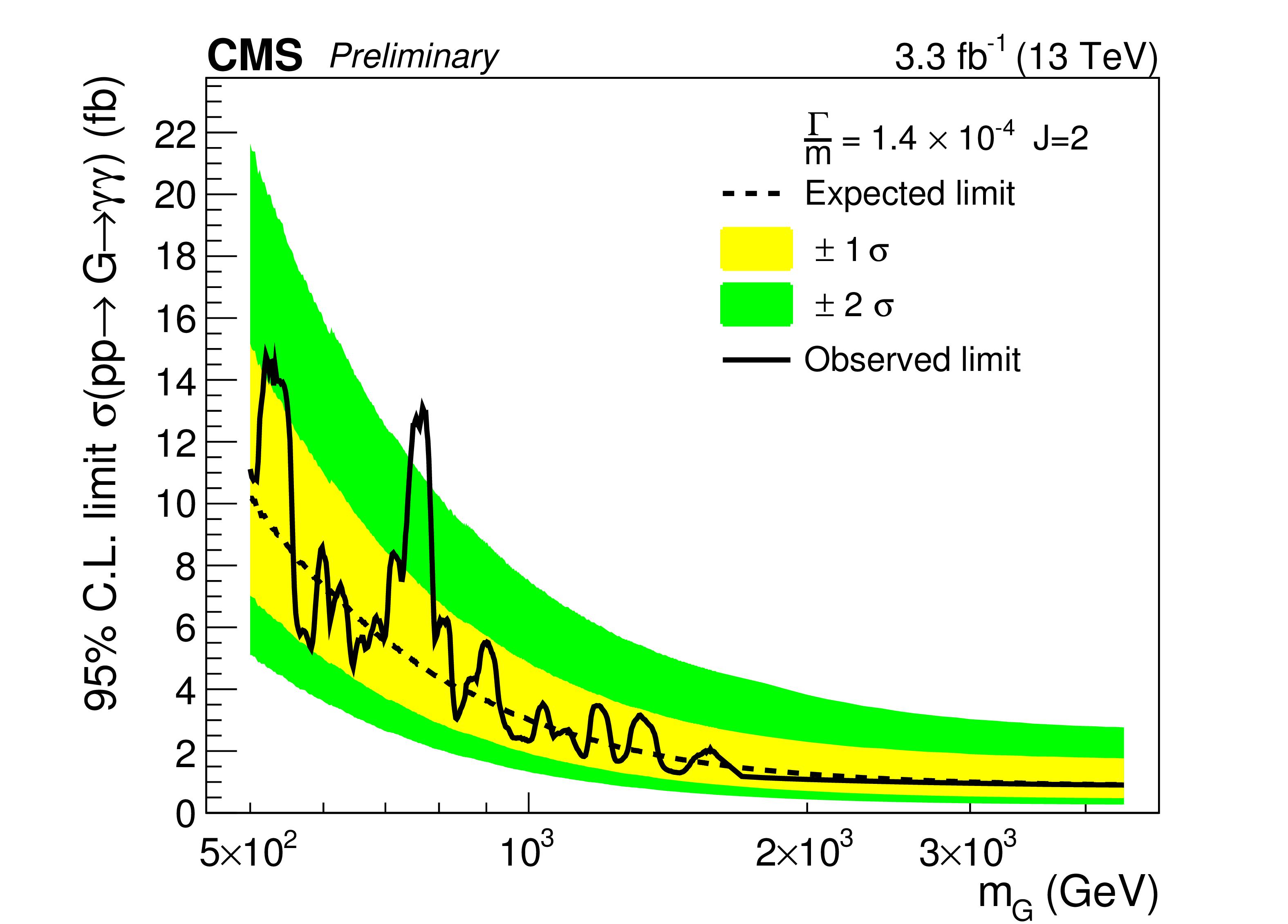
png pdf	Figure 5-b: Expected and observed 95% C.L. exclusion limits for different signal hypotheses. The range 500 GeV $< m <$ 4.5 TeV is shown for ${\Gamma / m} = 1.4\times 10^{-4}$ , $1.4\times 10^{-2}$ , $5.6\times 10^{-2}$ . The (a,c) (b,d) column corresponds to the scalar (RS graviton) signals.
png pdf	Figure 5-c: Expected and observed 95% C.L. exclusion limits for different signal hypotheses. The range 500 GeV $< m <$ 4.5 TeV is shown for ${\Gamma / m} = 1.4\times 10^{-4}$ , $1.4\times 10^{-2}$ , $5.6\times 10^{-2}$ . The (a,c) (b,d) column corresponds to the scalar (RS graviton) signals.
png pdf	Figure 5-d: Expected and observed 95% C.L. exclusion limits for different signal hypotheses. The range 500 GeV $< m <$ 4.5 TeV is shown for ${\Gamma / m} = 1.4\times 10^{-4}$ , $1.4\times 10^{-2}$ , $5.6\times 10^{-2}$ . The (a,c) (b,d) column corresponds to the scalar (RS graviton) signals.
png pdf	Figure 5-e: Expected and observed 95% C.L. exclusion limits for different signal hypotheses. The range 500 GeV $< m <$ 4.5 TeV is shown for ${\Gamma / m} = 1.4\times 10^{-4}$ , $1.4\times 10^{-2}$ , $5.6\times 10^{-2}$ . The (a,c) (b,d) column corresponds to the scalar (RS graviton) signals.
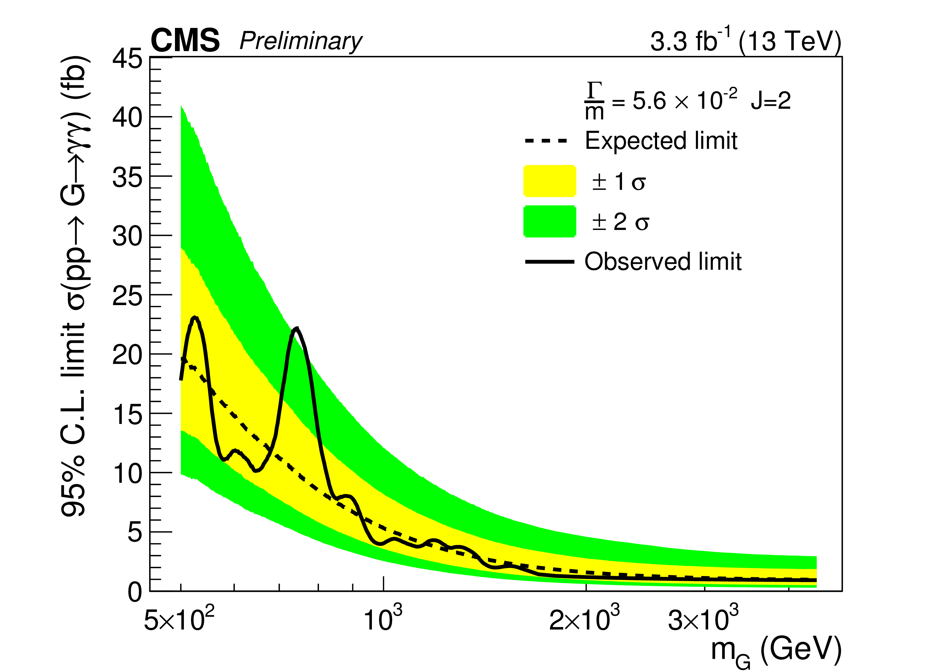
png pdf	Figure 5-f: Expected and observed 95% C.L. exclusion limits for different signal hypotheses. The range 500 GeV $< m <$ 4.5 TeV is shown for ${\Gamma / m} = 1.4\times 10^{-4}$ , $1.4\times 10^{-2}$ , $5.6\times 10^{-2}$ . The (a,c) (b,d) column corresponds to the scalar (RS graviton) signals.
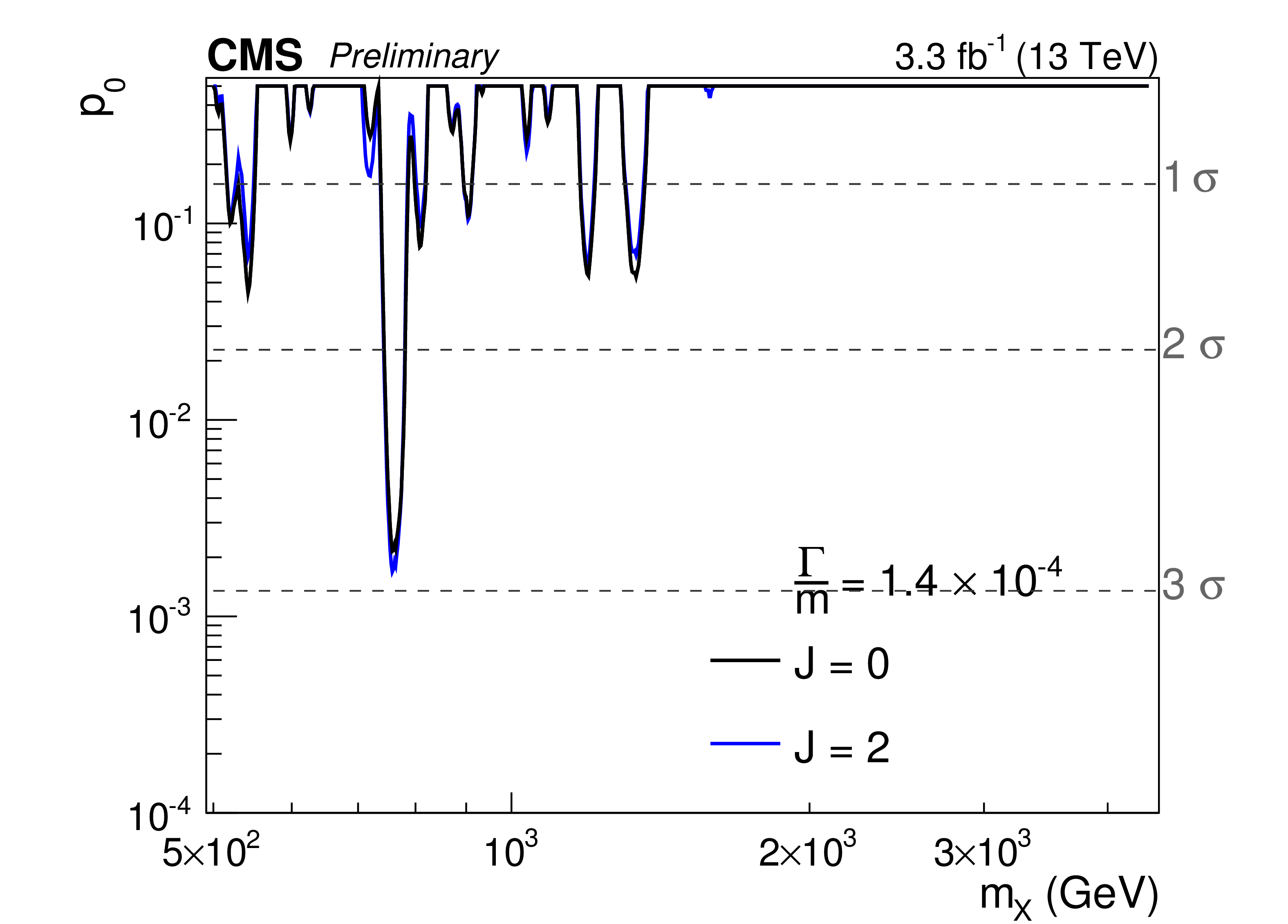
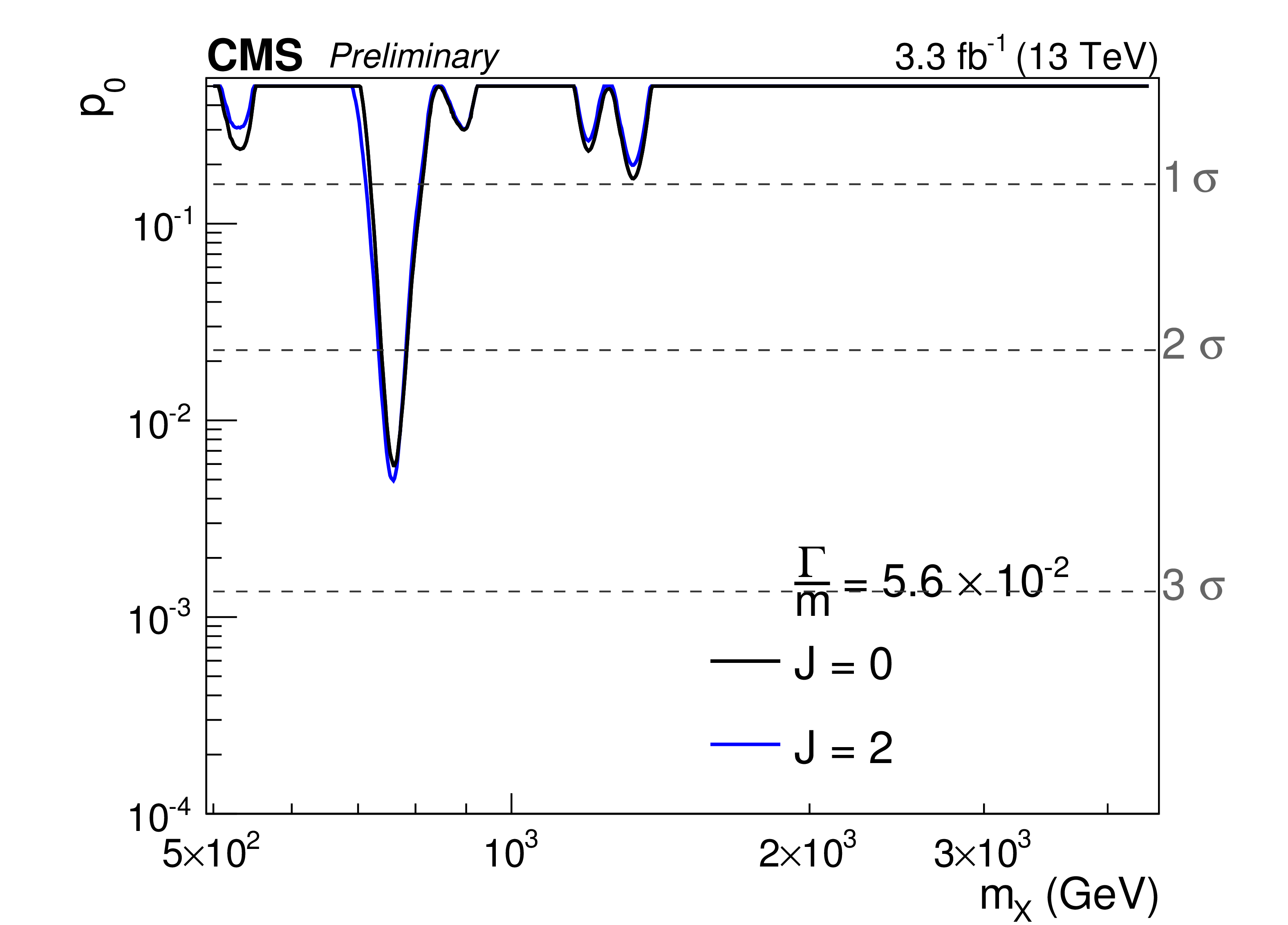
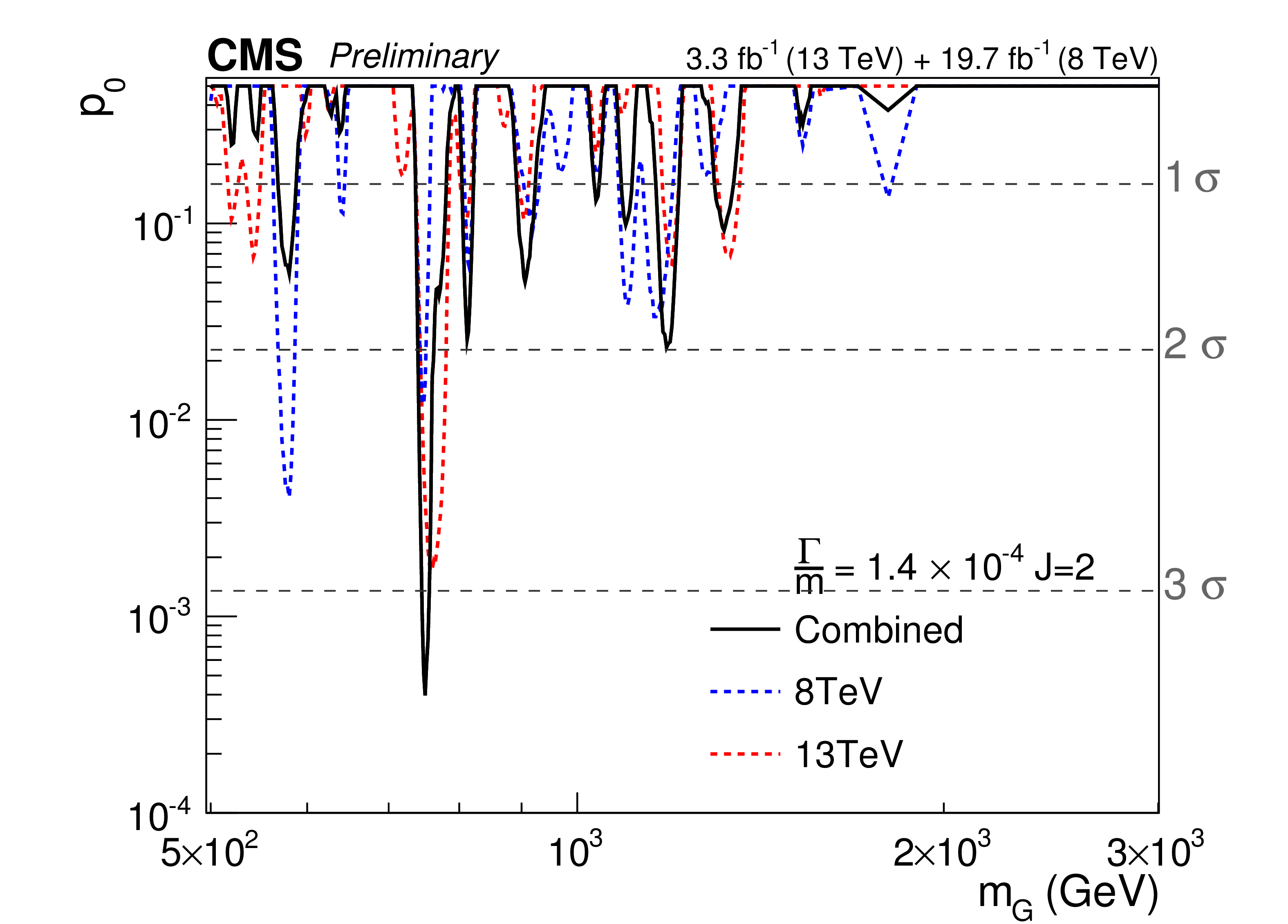
png pdf	Figure 6-a: Observed background-only $p$ -value for different signal hypotheses. The range 500 GeV $< m <$ 4.5 TeV is shown for ${\Gamma / m} = 1.4\times 10^{-4}$ , $1.4\times 10^{-2}$ , $5.6\times 10^{-2}$ . Results corresponding to both the scalar and RS graviton hypotheses are shown.
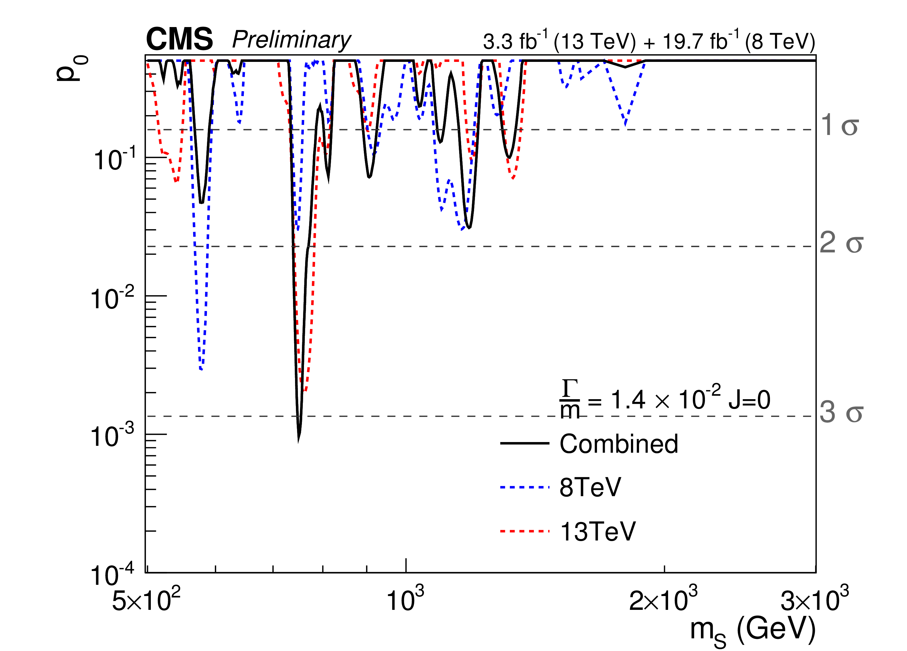
png pdf	Figure 6-b: Observed background-only $p$ -value for different signal hypotheses. The range 500 GeV $< m <$ 4.5 TeV is shown for ${\Gamma / m} = 1.4\times 10^{-4}$ , $1.4\times 10^{-2}$ , $5.6\times 10^{-2}$ . Results corresponding to both the scalar and RS graviton hypotheses are shown.
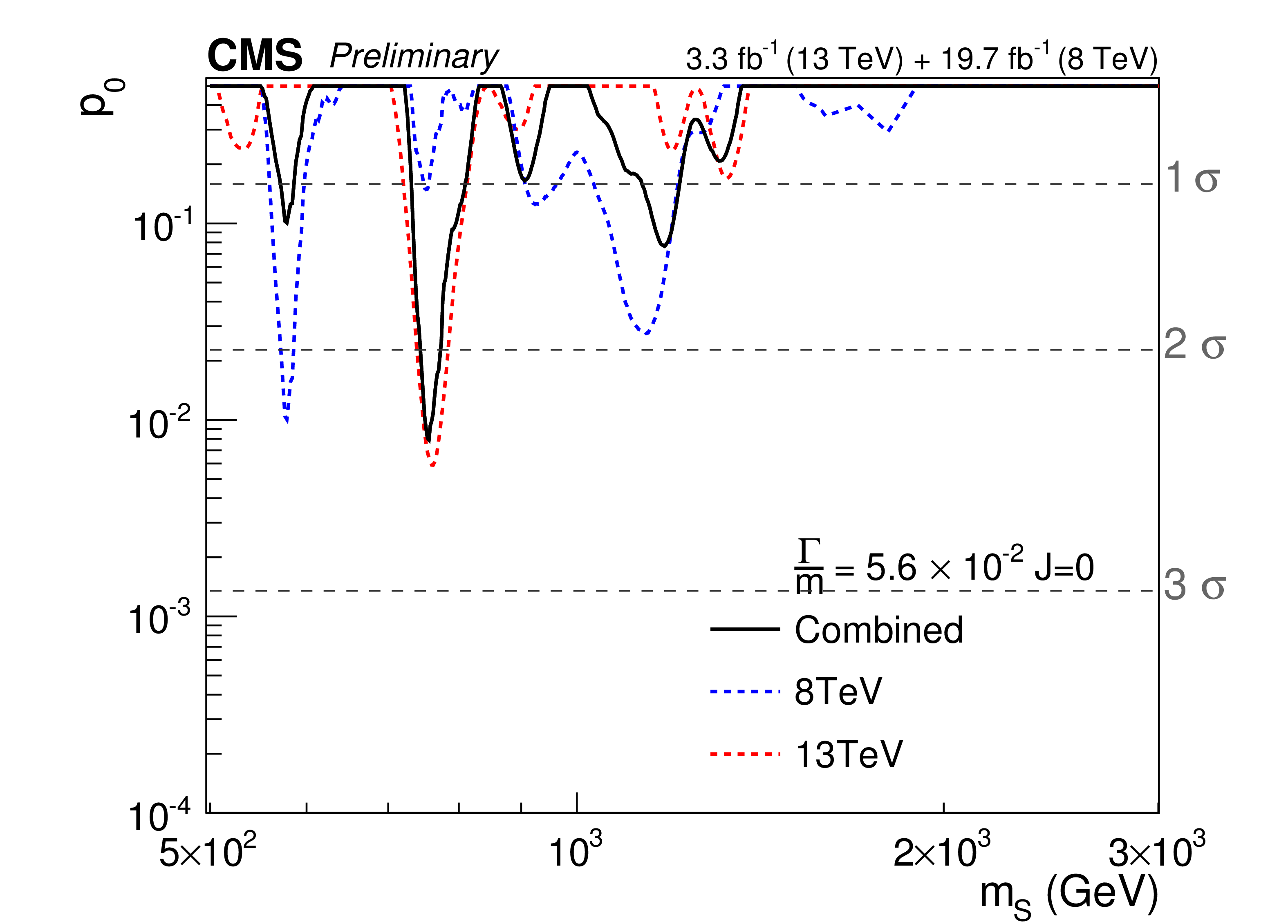
png pdf	Figure 6-c: Observed background-only $p$ -value for different signal hypotheses. The range 500 GeV $< m <$ 4.5 TeV is shown for ${\Gamma / m} = 1.4\times 10^{-4}$ , $1.4\times 10^{-2}$ , $5.6\times 10^{-2}$ . Results corresponding to both the scalar and RS graviton hypotheses are shown.
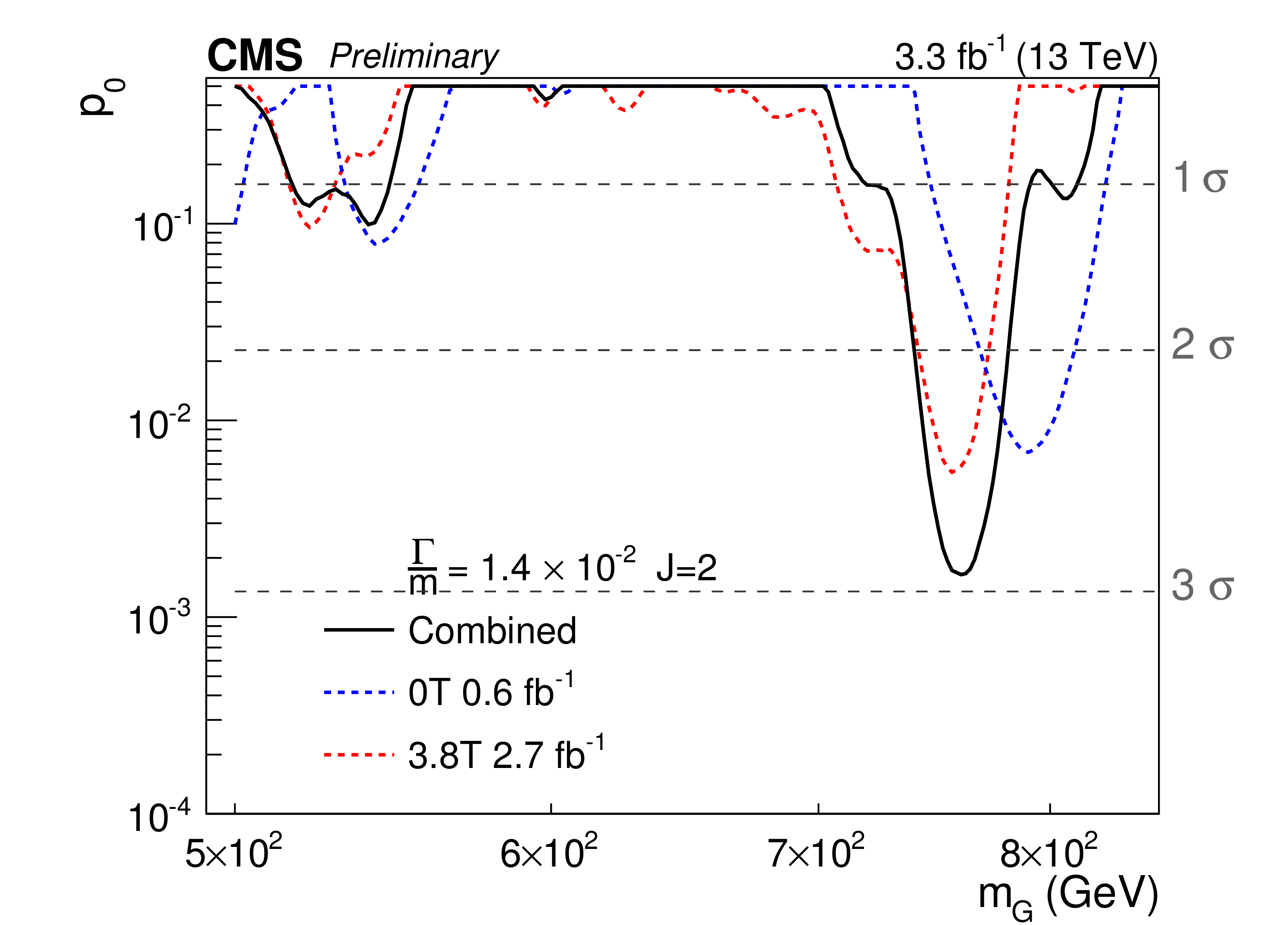
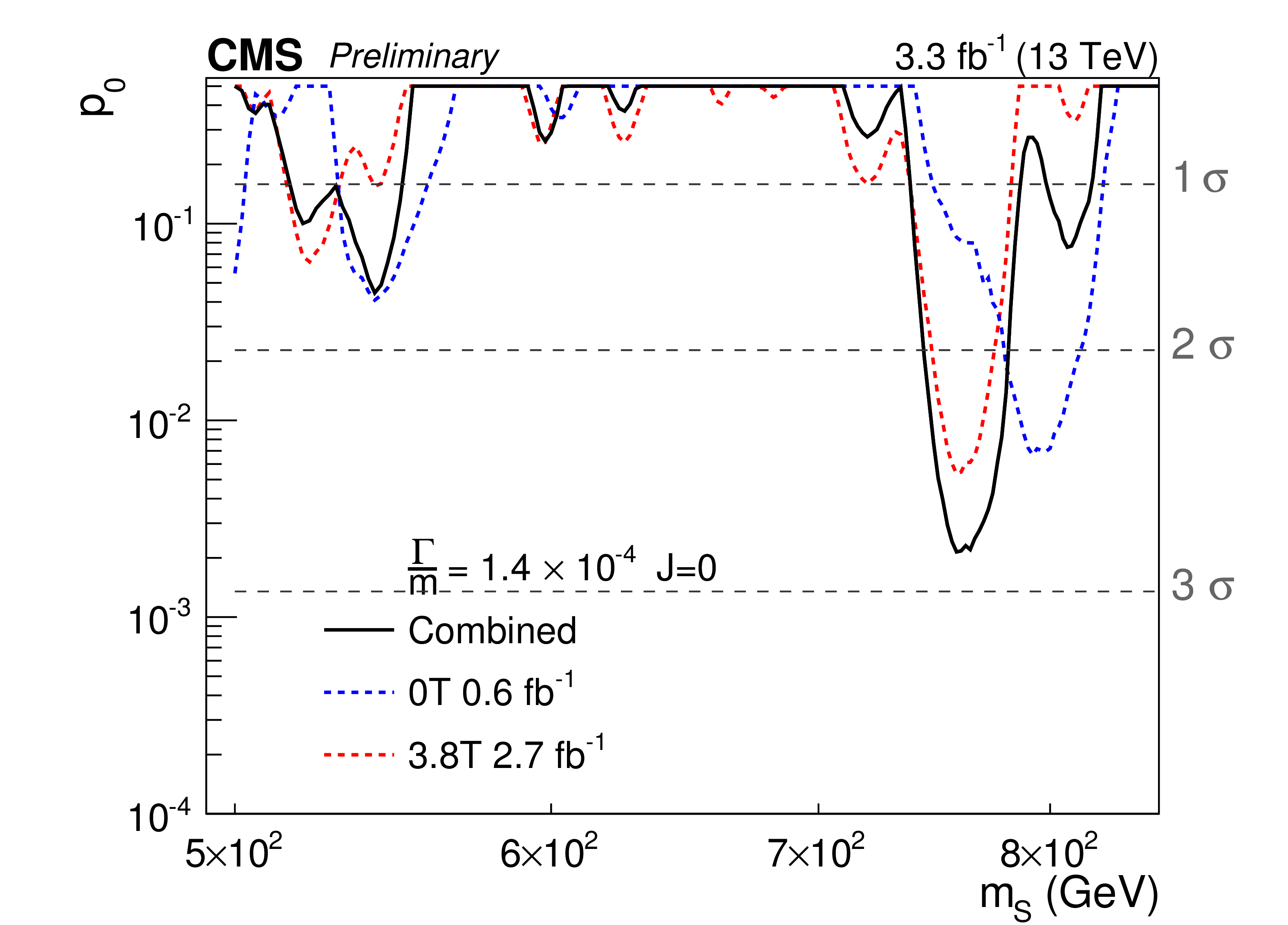
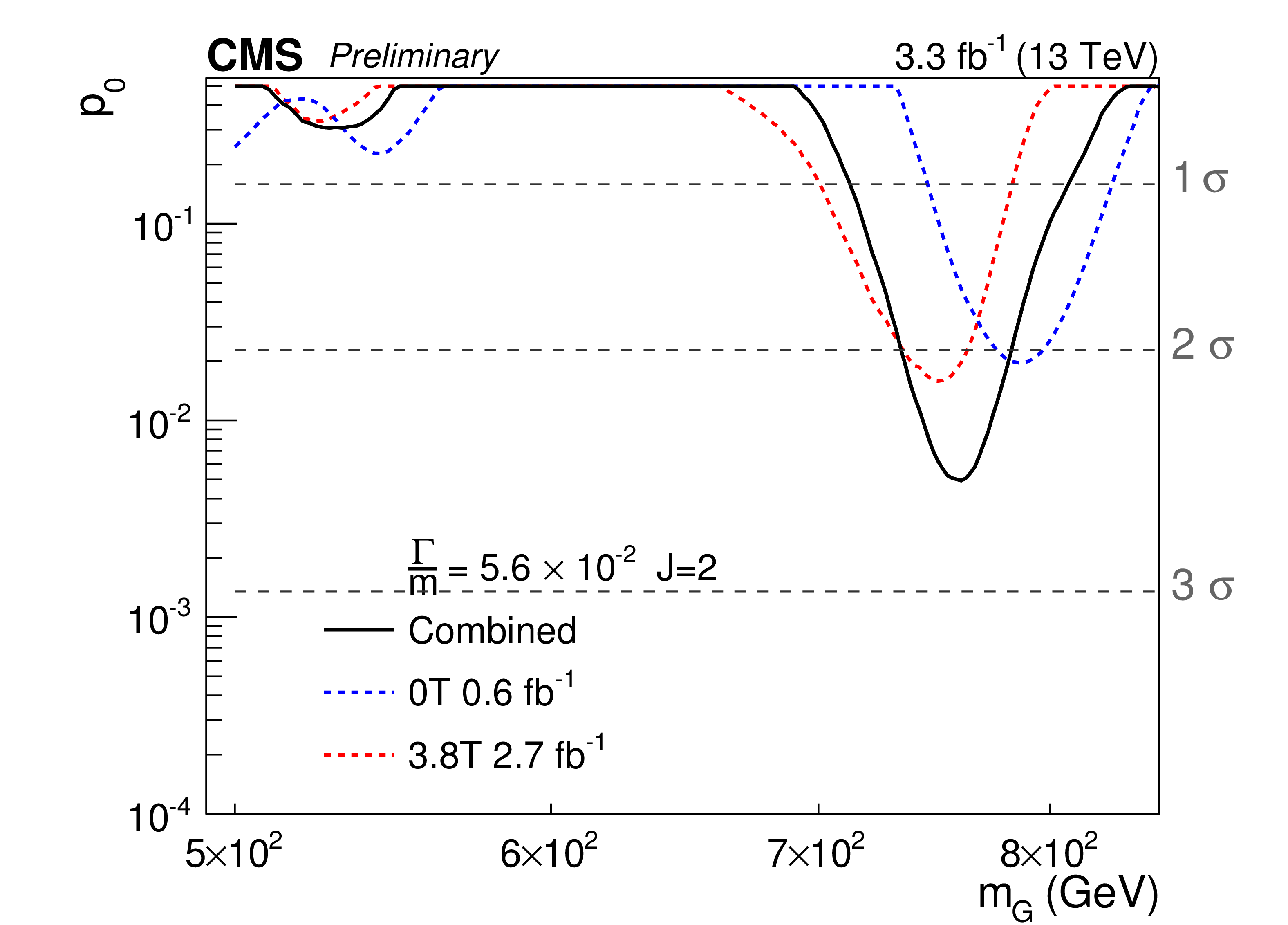
png pdf	Figure 7-a: Observed background only $p$ -values obtained on the 13 TeV dataset. The mass range 500 GeV $< {m} <$ 850 GeV is shown is for resonances of ${\Gamma / m} = 1.4\times 10^{-2}$ . The contributions of the B = 3.8 T and B = 0 T datasets are shown separately. Due to the different size of the two datasets, the weight of the B = 0 T categories in the combined result is, at ${m} =$ 760 GeV, roughly one fifth of that of the B = 3.8 T ones. The a (b) plot corresponds to the scalar (RS graviton) hypotheses.
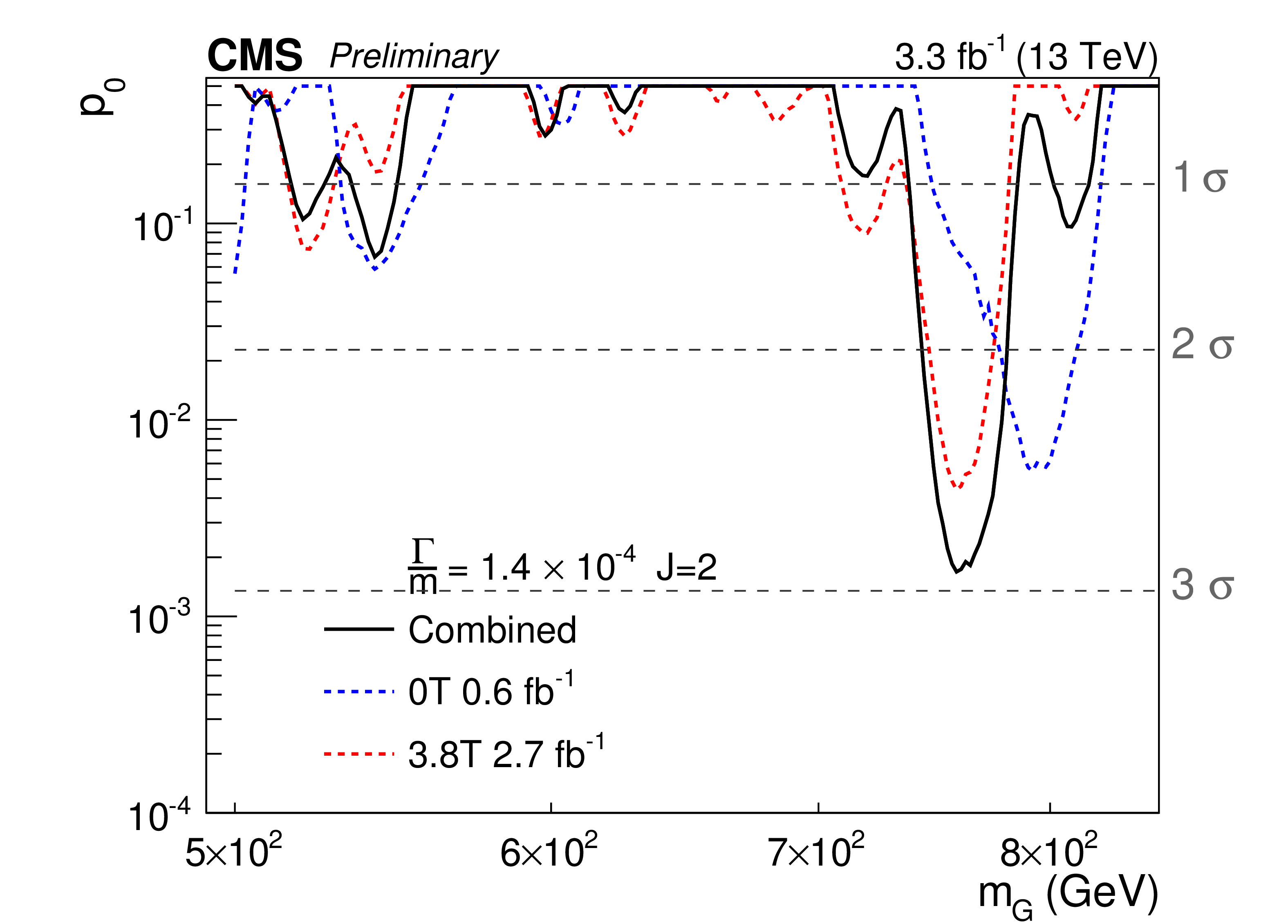
png pdf	Figure 7-b: Observed background only $p$ -values obtained on the 13 TeV dataset. The mass range 500 GeV $< {m} <$ 850 GeV is shown is for resonances of ${\Gamma / m} = 1.4\times 10^{-2}$ . The contributions of the B = 3.8 T and B = 0 T datasets are shown separately. Due to the different size of the two datasets, the weight of the B = 0 T categories in the combined result is, at ${m} =$ 760 GeV, roughly one fifth of that of the B = 3.8 T ones. The a (b) plot corresponds to the scalar (RS graviton) hypotheses.
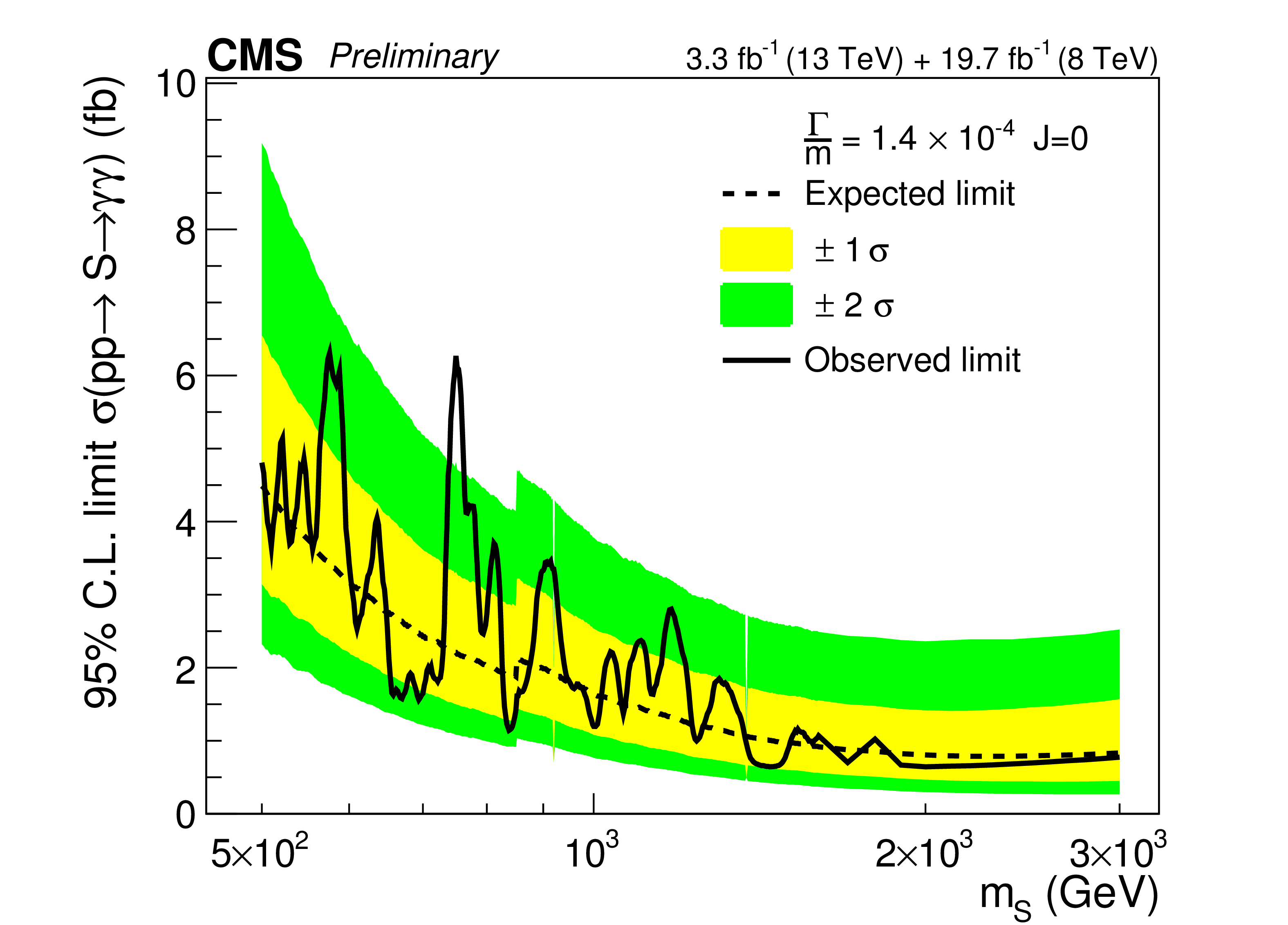
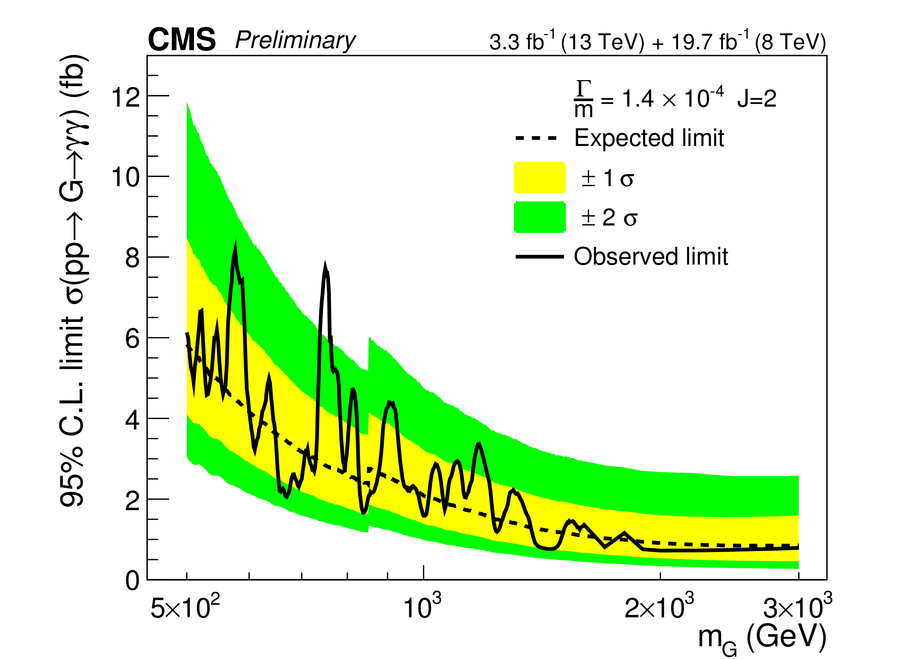
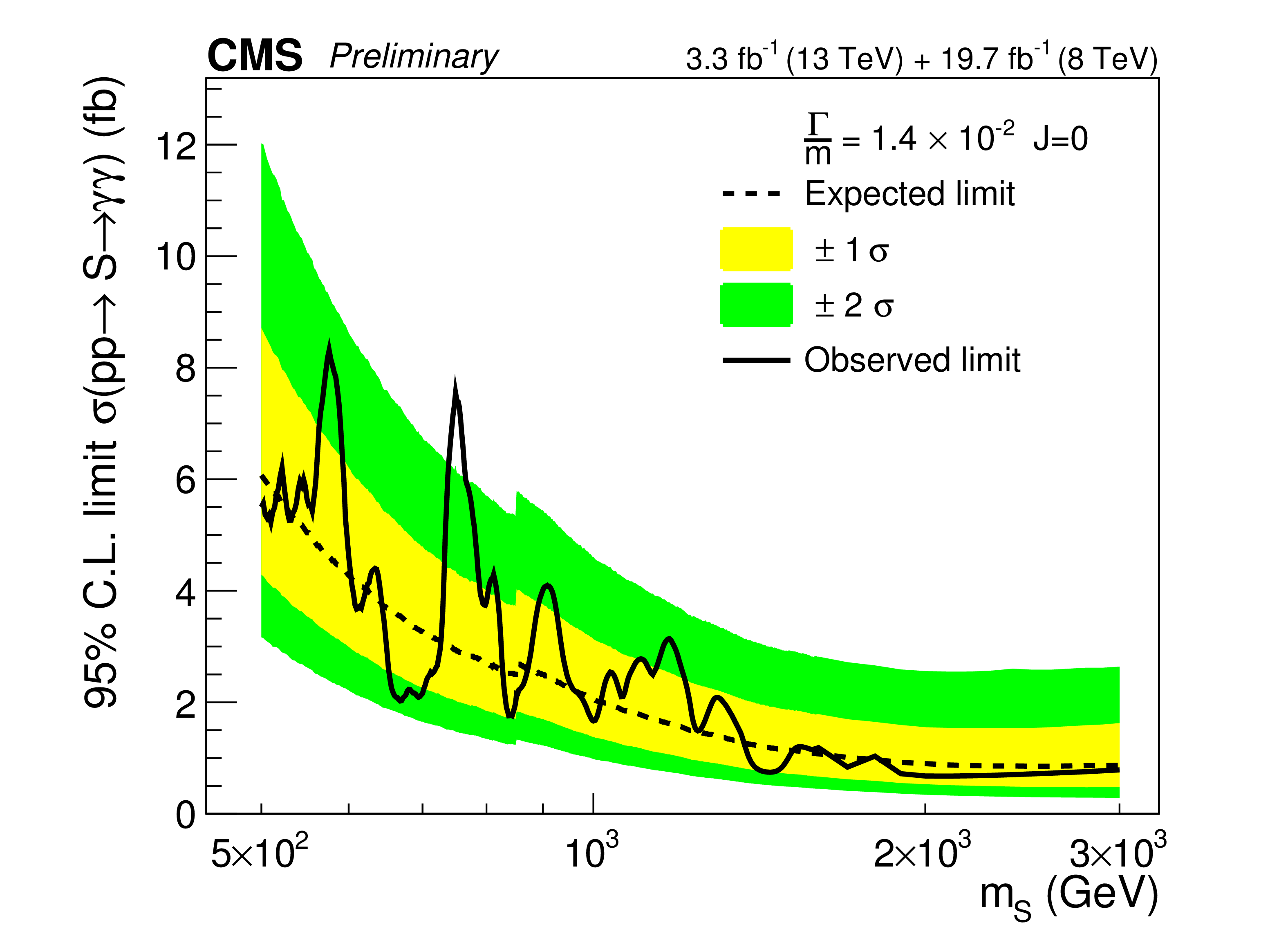
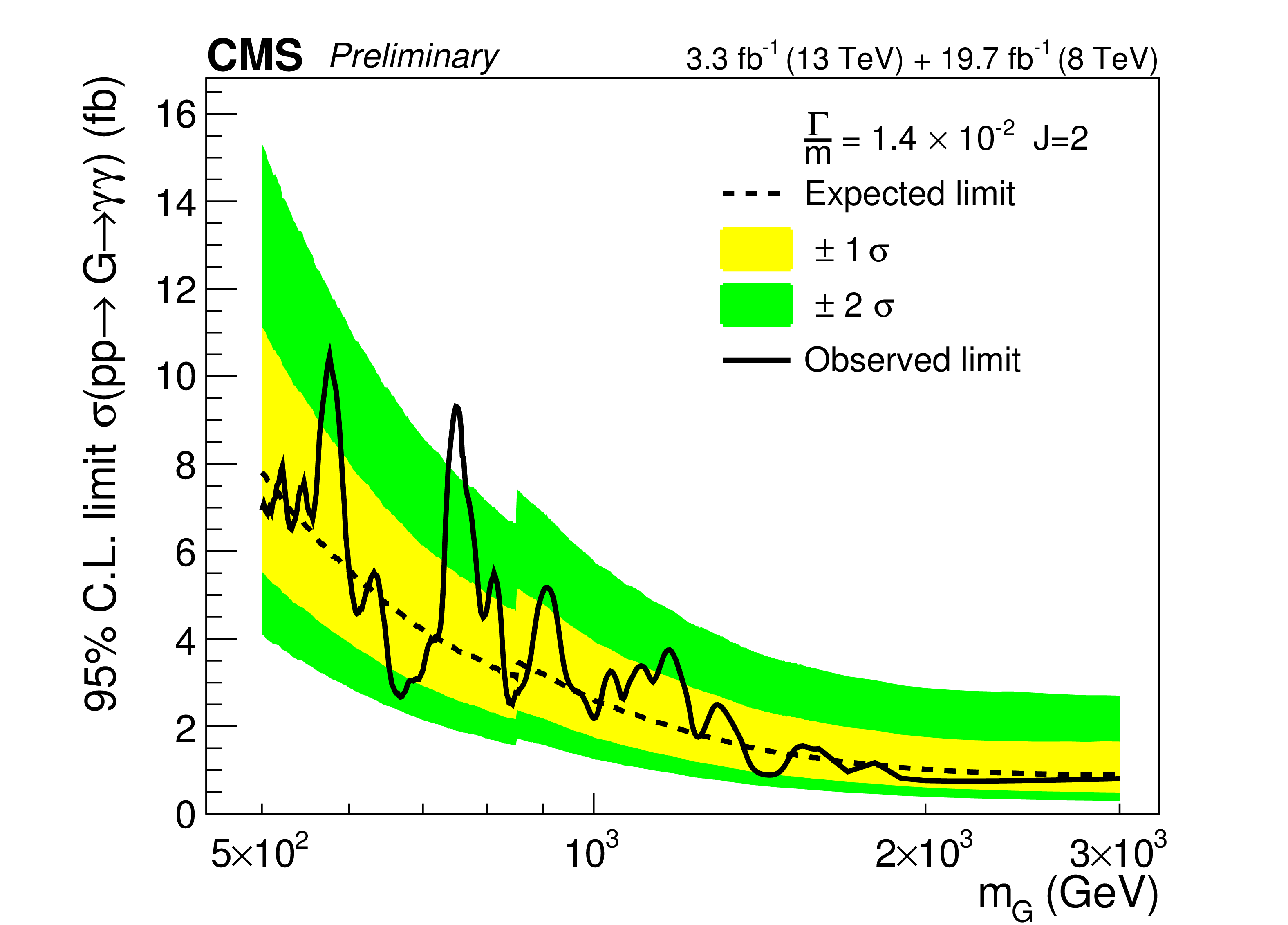
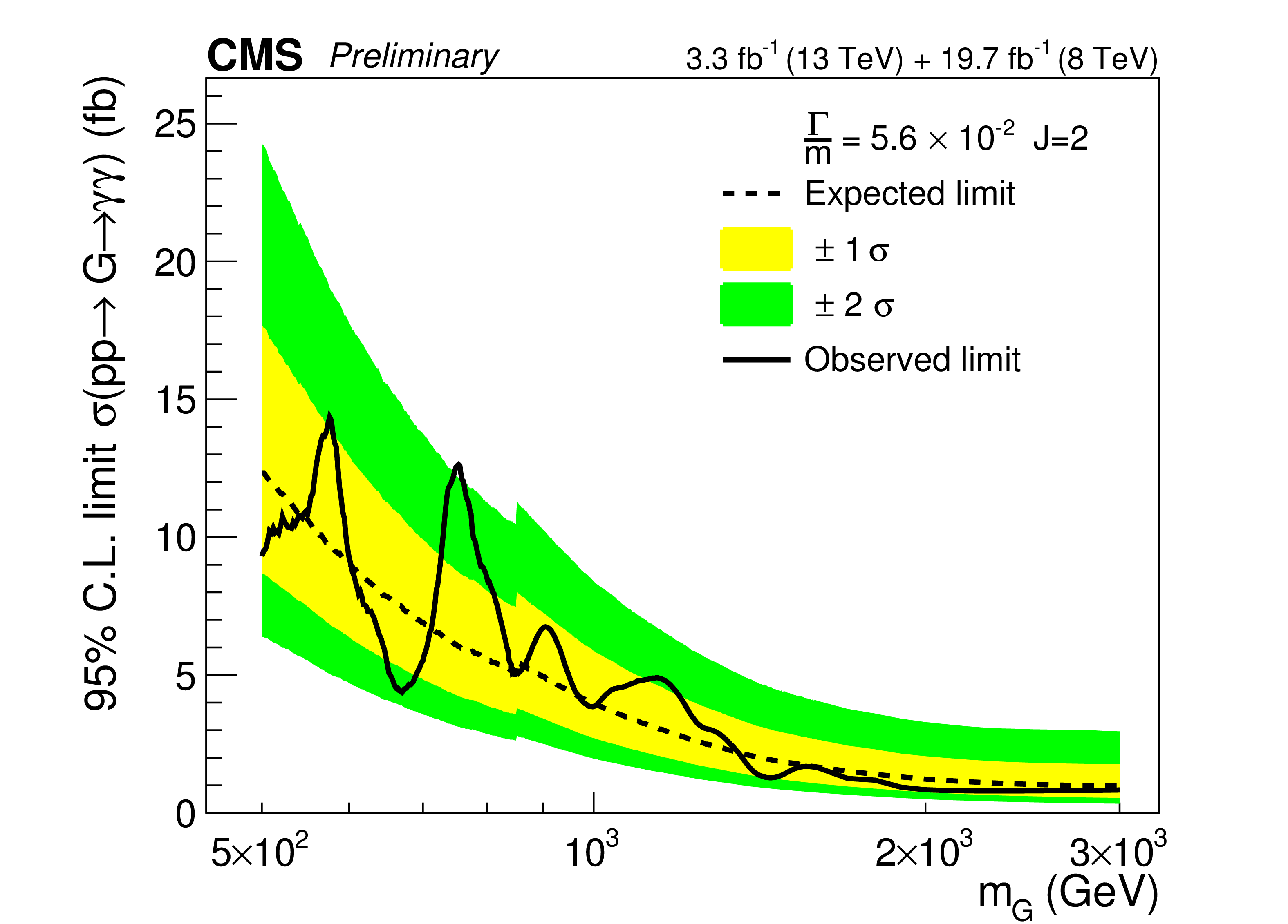
png pdf	Figure 8-a: Upper limits on the production of high mass diphoton resonances obtained with the combined analysis of the 8 and 13 TeV data. The a,c,e (b,d,f) column corresponds to the scalar (RS graviton) signals. For ${m} <$ 850 GeV, the results obtained at ${\sqrt {s}} =$ 8 TeV with the analysis described in Ref.[16] are combined with those obtained at ${\sqrt {s}} =$ 13 TeV. For ${m} >$ 850 GeV the results of the analysis described in Ref.[17] obtained at 8 TeV are combined with those obtained at $\sqrt {s} =$ 13 TeV.
png pdf	Figure 8-b: Upper limits on the production of high mass diphoton resonances obtained with the combined analysis of the 8 and 13 TeV data. The a,c,e (b,d,f) column corresponds to the scalar (RS graviton) signals. For ${m} <$ 850 GeV, the results obtained at ${\sqrt {s}} =$ 8 TeV with the analysis described in Ref.[16] are combined with those obtained at ${\sqrt {s}} =$ 13 TeV. For ${m} >$ 850 GeV the results of the analysis described in Ref.[17] obtained at 8 TeV are combined with those obtained at $\sqrt {s} =$ 13 TeV.
png pdf	Figure 8-c: Upper limits on the production of high mass diphoton resonances obtained with the combined analysis of the 8 and 13 TeV data. The a,c,e (b,d,f) column corresponds to the scalar (RS graviton) signals. For ${m} <$ 850 GeV, the results obtained at ${\sqrt {s}} =$ 8 TeV with the analysis described in Ref.[16] are combined with those obtained at ${\sqrt {s}} =$ 13 TeV. For ${m} >$ 850 GeV the results of the analysis described in Ref.[17] obtained at 8 TeV are combined with those obtained at $\sqrt {s} =$ 13 TeV.
png pdf	Figure 8-d: Upper limits on the production of high mass diphoton resonances obtained with the combined analysis of the 8 and 13 TeV data. The a,c,e (b,d,f) column corresponds to the scalar (RS graviton) signals. For ${m} <$ 850 GeV, the results obtained at ${\sqrt {s}} =$ 8 TeV with the analysis described in Ref.[16] are combined with those obtained at ${\sqrt {s}} =$ 13 TeV. For ${m} >$ 850 GeV the results of the analysis described in Ref.[17] obtained at 8 TeV are combined with those obtained at $\sqrt {s} =$ 13 TeV.
png pdf	Figure 8-e: Upper limits on the production of high mass diphoton resonances obtained with the combined analysis of the 8 and 13 TeV data. The a,c,e (b,d,f) column corresponds to the scalar (RS graviton) signals. For ${m} <$ 850 GeV, the results obtained at ${\sqrt {s}} =$ 8 TeV with the analysis described in Ref.[16] are combined with those obtained at ${\sqrt {s}} =$ 13 TeV. For ${m} >$ 850 GeV the results of the analysis described in Ref.[17] obtained at 8 TeV are combined with those obtained at $\sqrt {s} =$ 13 TeV.
png pdf	Figure 8-f: Upper limits on the production of high mass diphoton resonances obtained with the combined analysis of the 8 and 13 TeV data. The a,c,e (b,d,f) column corresponds to the scalar (RS graviton) signals. For ${m} <$ 850 GeV, the results obtained at ${\sqrt {s}} =$ 8 TeV with the analysis described in Ref.[16] are combined with those obtained at ${\sqrt {s}} =$ 13 TeV. For ${m} >$ 850 GeV the results of the analysis described in Ref.[17] obtained at 8 TeV are combined with those obtained at $\sqrt {s} =$ 13 TeV.
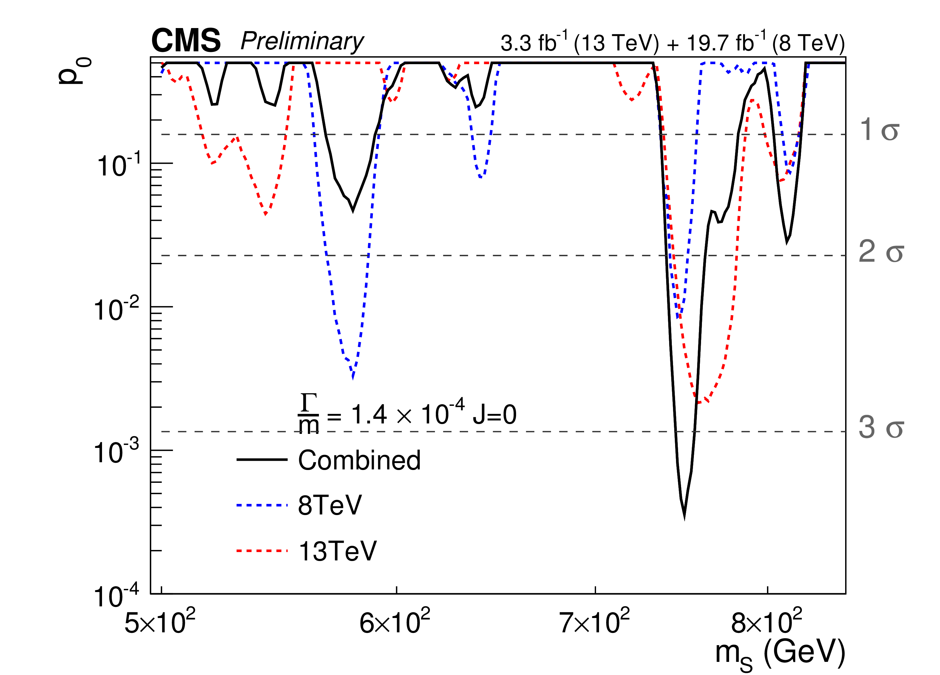
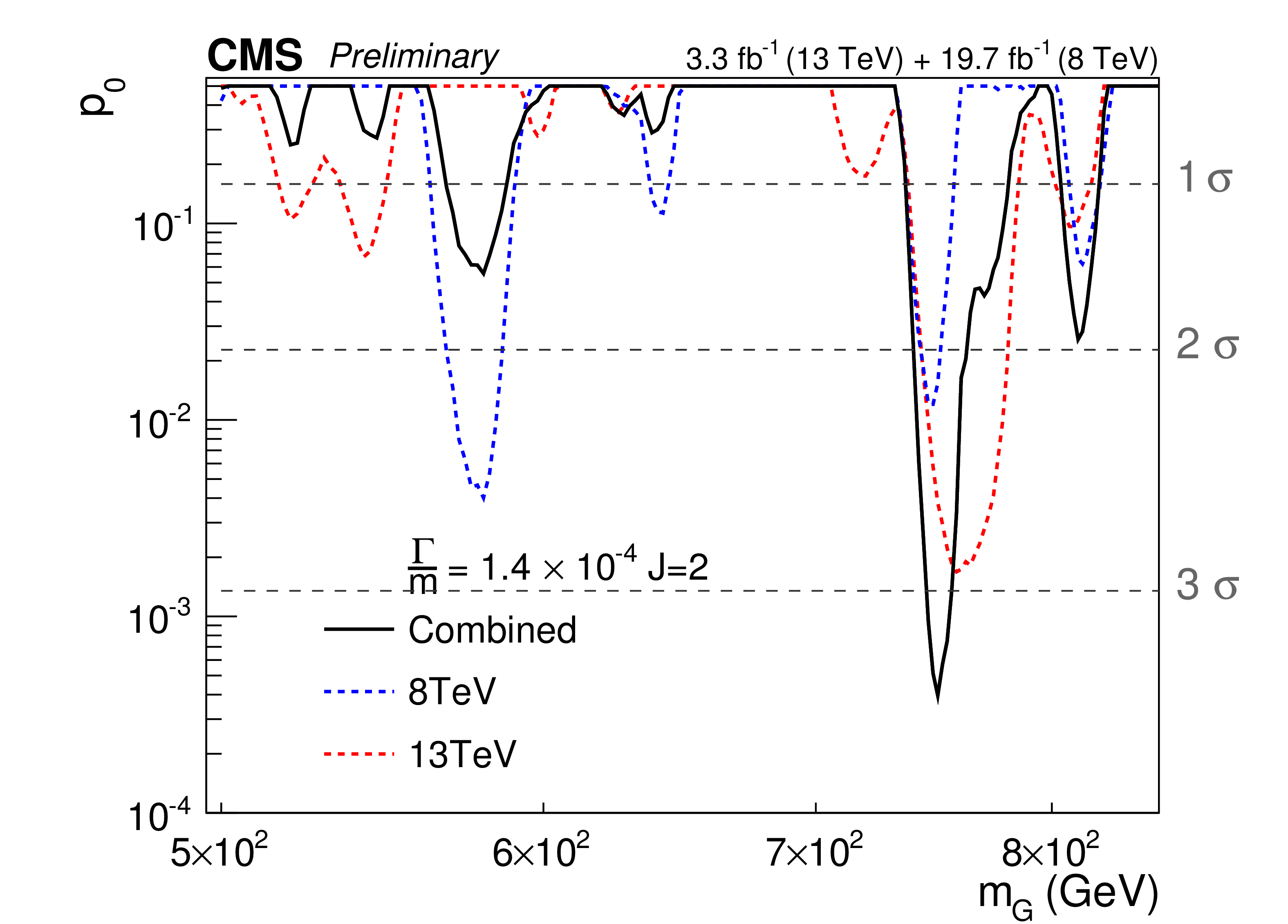
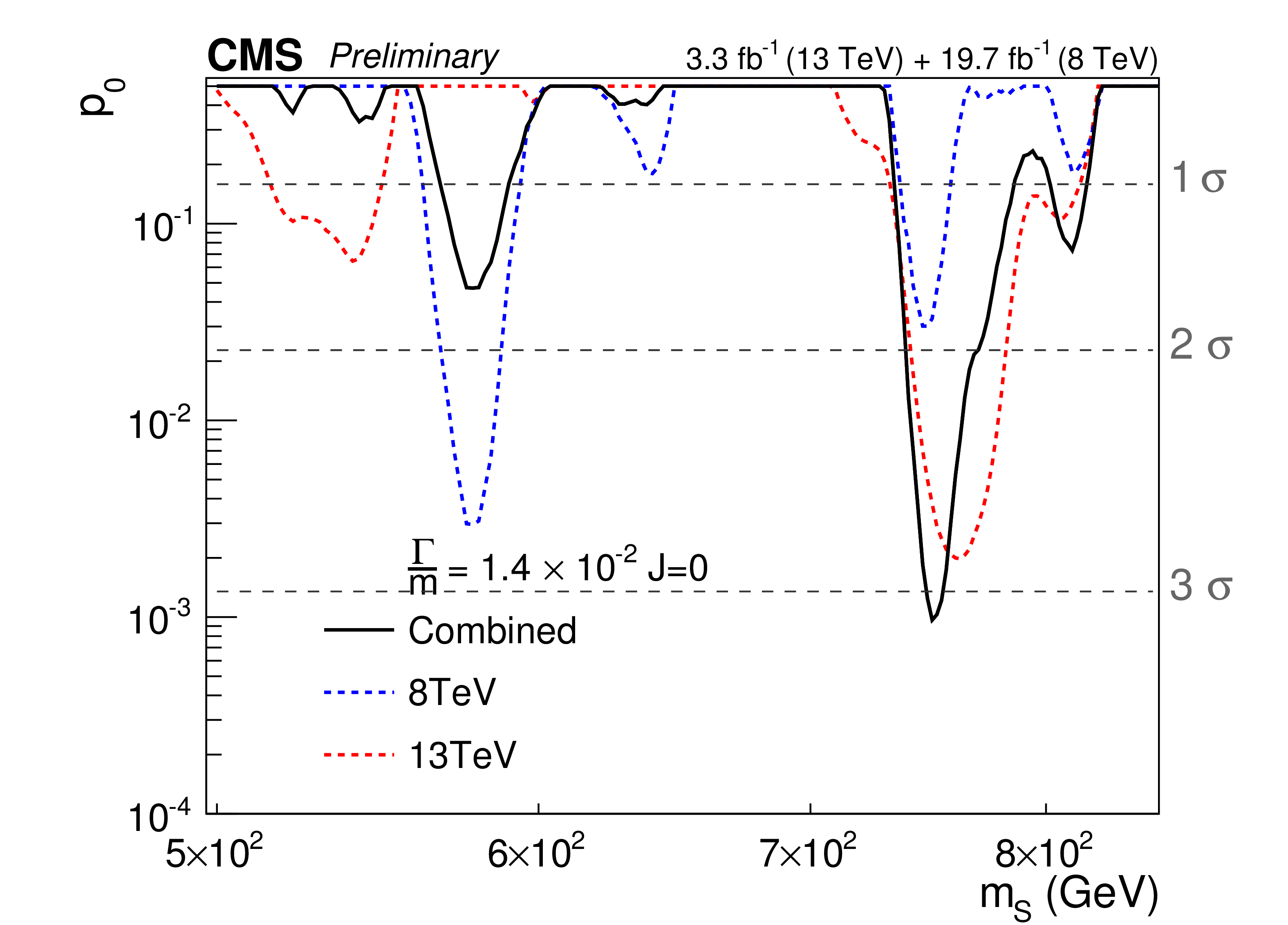
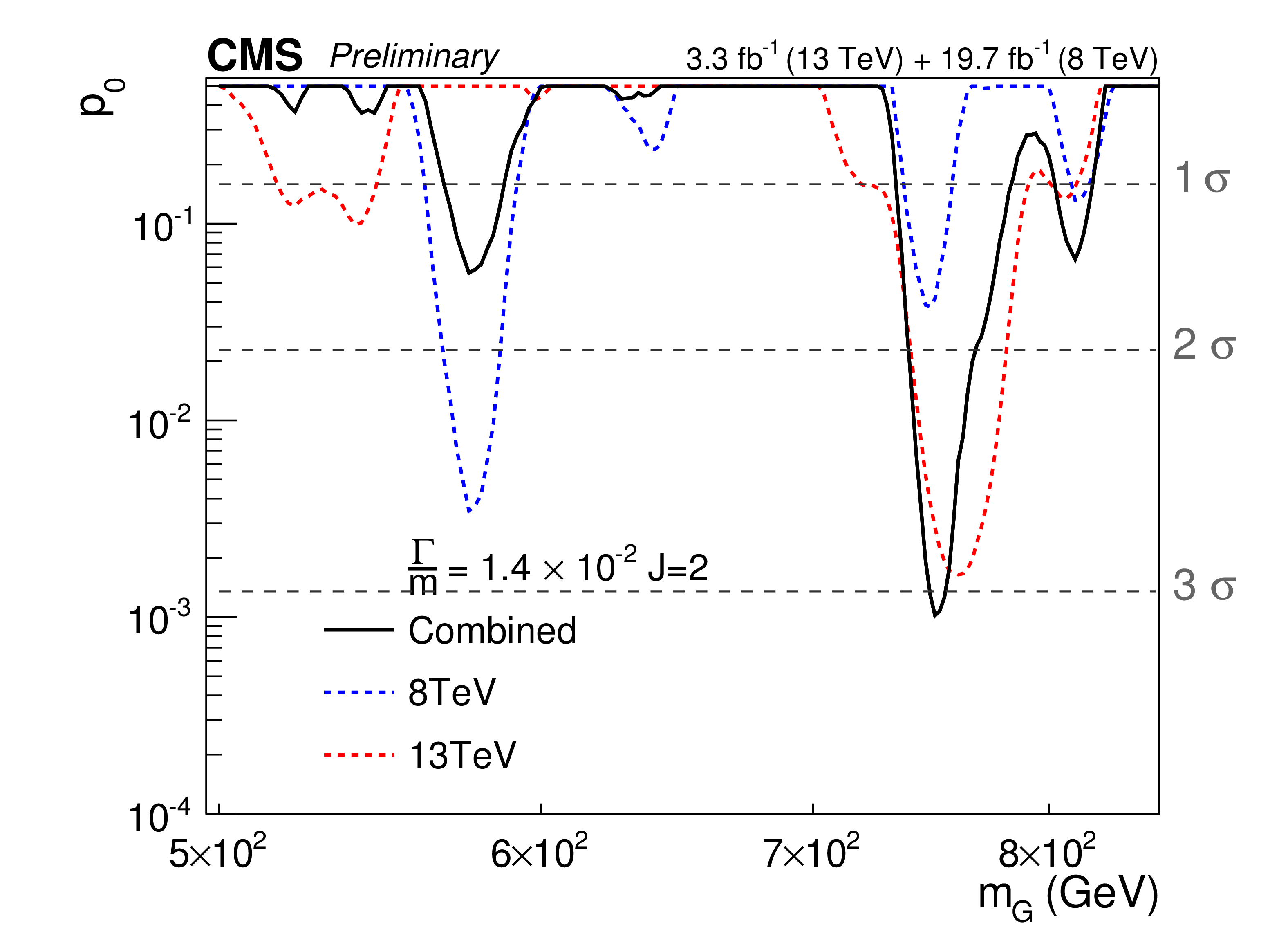
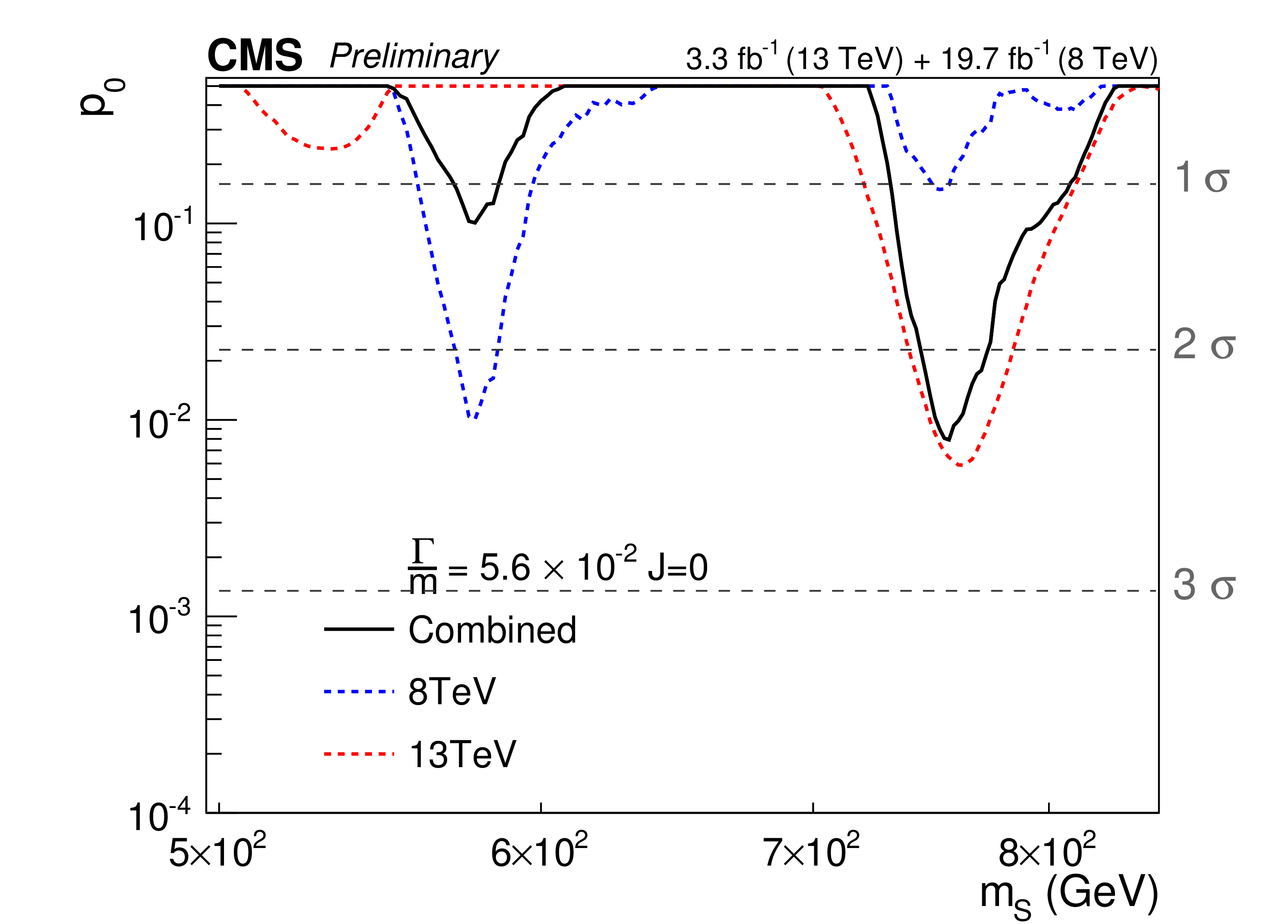
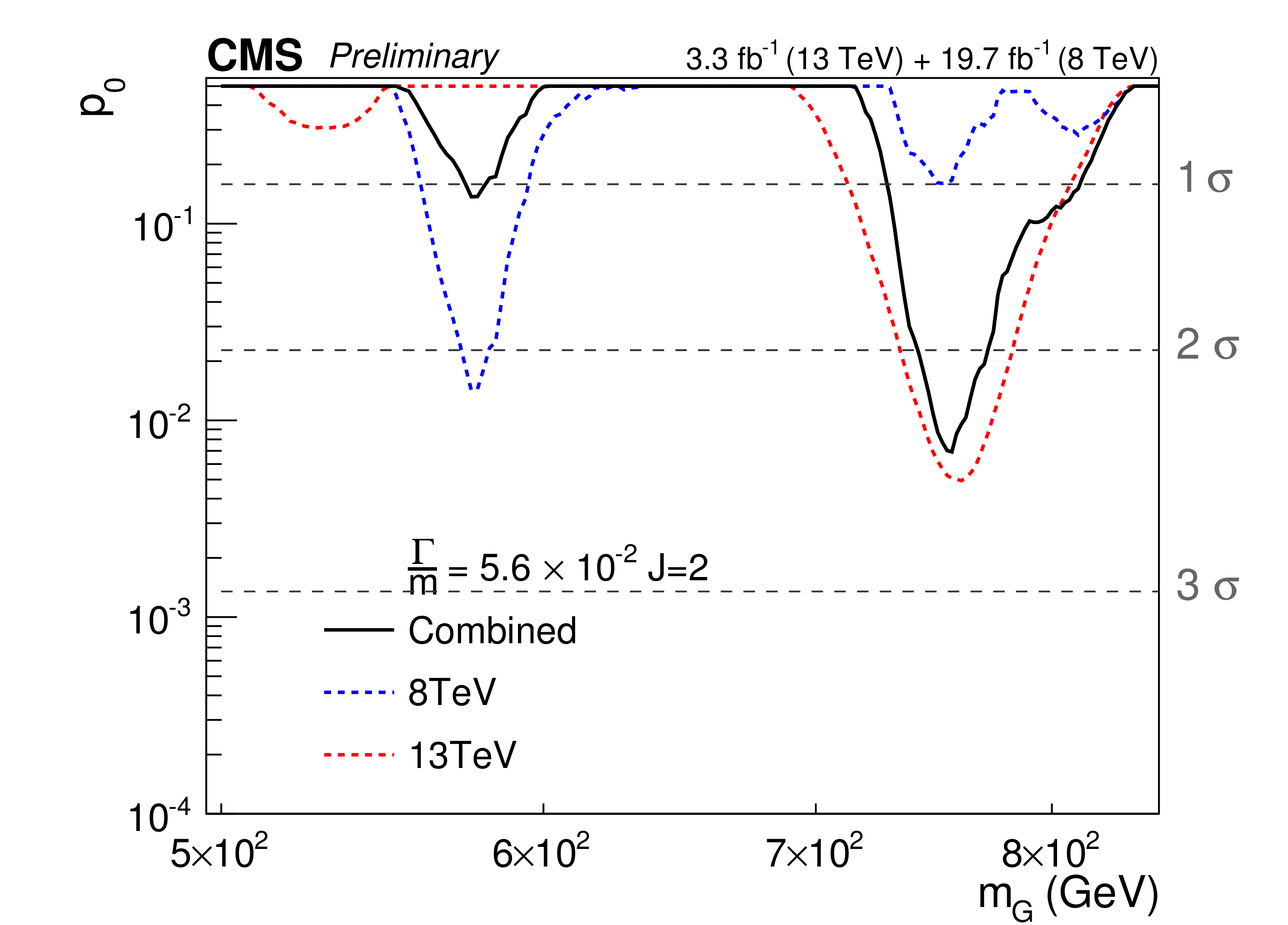
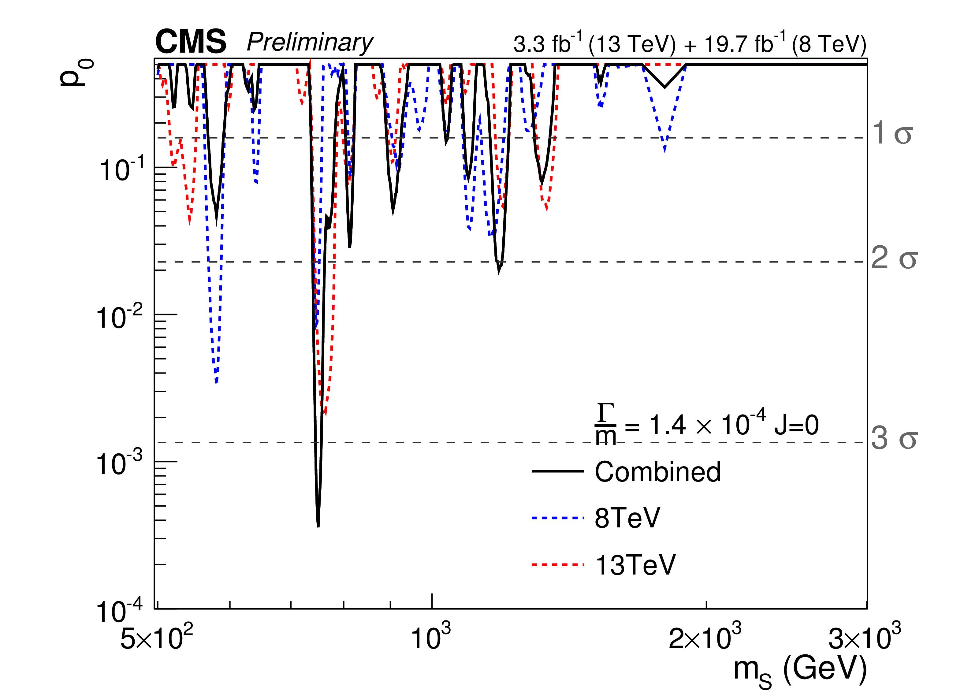
png pdf	Figure 9-a: Observed background only p-values obtained from the combination of 8 TeV and 13 TeV results for different signal hypotheses. The contributions of the 8 and 13 TeV datasets are shown separately. At ${m} =$ 750 GeV, the two datasets contribute with similar weights to the combined result. The a,c,e (b,d,f) column corresponds to the scalar (RS graviton) signals.
png pdf	Figure 9-b: Observed background only p-values obtained from the combination of 8 TeV and 13 TeV results for different signal hypotheses. The contributions of the 8 and 13 TeV datasets are shown separately. At ${m} =$ 750 GeV, the two datasets contribute with similar weights to the combined result. The a,c,e (b,d,f) column corresponds to the scalar (RS graviton) signals.
png pdf	Figure 9-c: Observed background only p-values obtained from the combination of 8 TeV and 13 TeV results for different signal hypotheses. The contributions of the 8 and 13 TeV datasets are shown separately. At ${m} =$ 750 GeV, the two datasets contribute with similar weights to the combined result. The a,c,e (b,d,f) column corresponds to the scalar (RS graviton) signals.
png pdf	Figure 9-d: Observed background only p-values obtained from the combination of 8 TeV and 13 TeV results for different signal hypotheses. The contributions of the 8 and 13 TeV datasets are shown separately. At ${m} =$ 750 GeV, the two datasets contribute with similar weights to the combined result. The a,c,e (b,d,f) column corresponds to the scalar (RS graviton) signals.
png pdf	Figure 9-e: Observed background only p-values obtained from the combination of 8 TeV and 13 TeV results for different signal hypotheses. The contributions of the 8 and 13 TeV datasets are shown separately. At ${m} =$ 750 GeV, the two datasets contribute with similar weights to the combined result. The a,c,e (b,d,f) column corresponds to the scalar (RS graviton) signals.
png pdf	Figure 9-f: Observed background only p-values obtained from the combination of 8 TeV and 13 TeV results for different signal hypotheses. The contributions of the 8 and 13 TeV datasets are shown separately. At ${m} =$ 750 GeV, the two datasets contribute with similar weights to the combined result. The a,c,e (b,d,f) column corresponds to the scalar (RS graviton) signals.
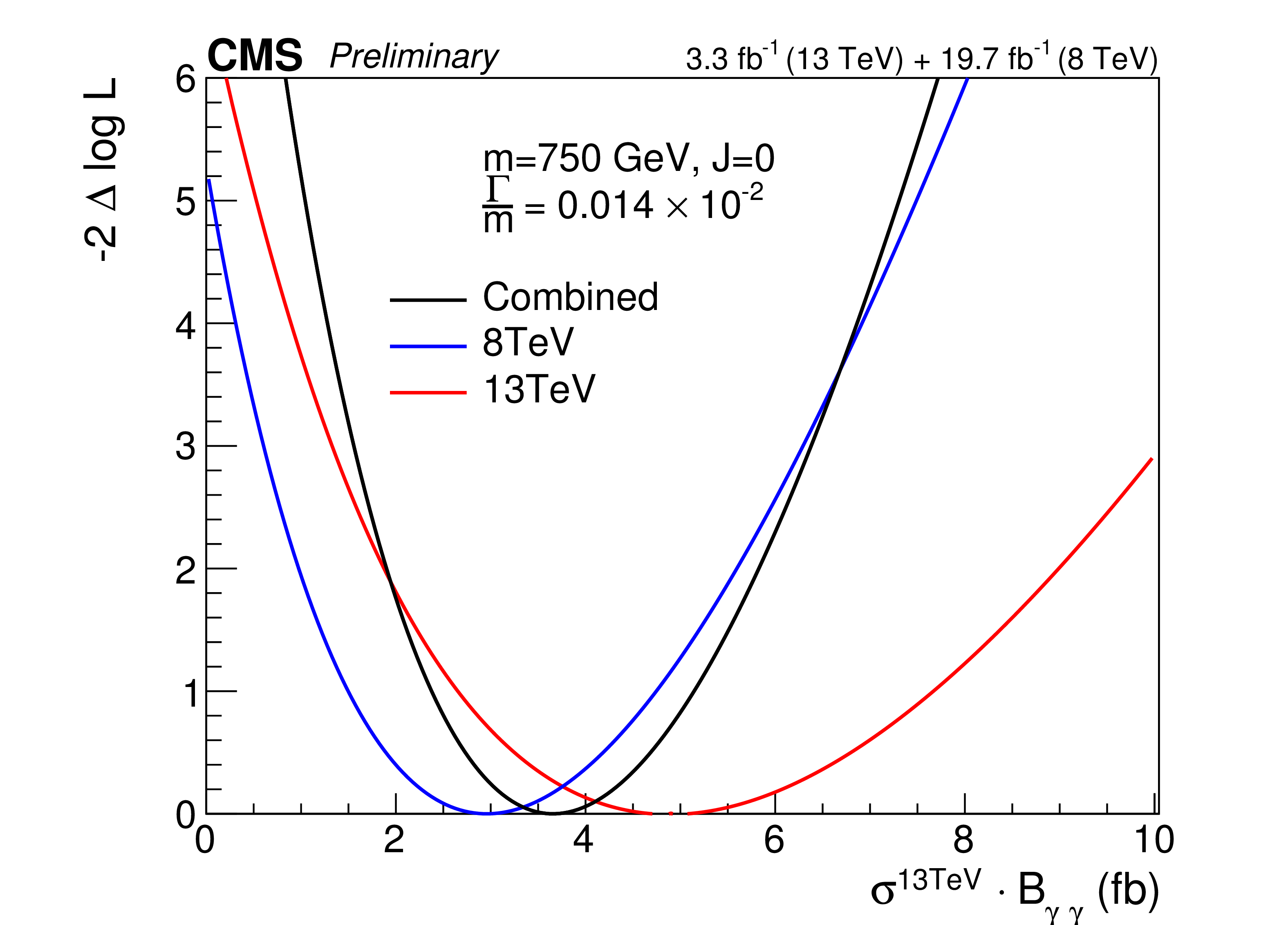
png pdf	Figure 10-a: Likelihood scan for the cross section corresponding to the largest excess in the combined analysis of the 8 and 13 TeV datasets. The a (b) plot corresponds to the scalar (RS graviton) signals. The 8 TeV results are scaled by the expected ratio of cross sections in each scenarios.
png pdf	Figure 10-b: Likelihood scan for the cross section corresponding to the largest excess in the combined analysis of the 8 and 13 TeV datasets. The a (b) plot corresponds to the scalar (RS graviton) signals. The 8 TeV results are scaled by the expected ratio of cross sections in each scenarios.

Tables
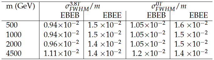
png pdf	Table 1: Intrinsic mass resolution, evaluated as ratio between the full width at half maximum of the ${m_{\gamma \gamma }}$ distribution, for narrow-width signals, and the its probable value, further divided by 2.35 as a function of the resonance mass for the event categories used in the analysis.

Auxiliary Figures
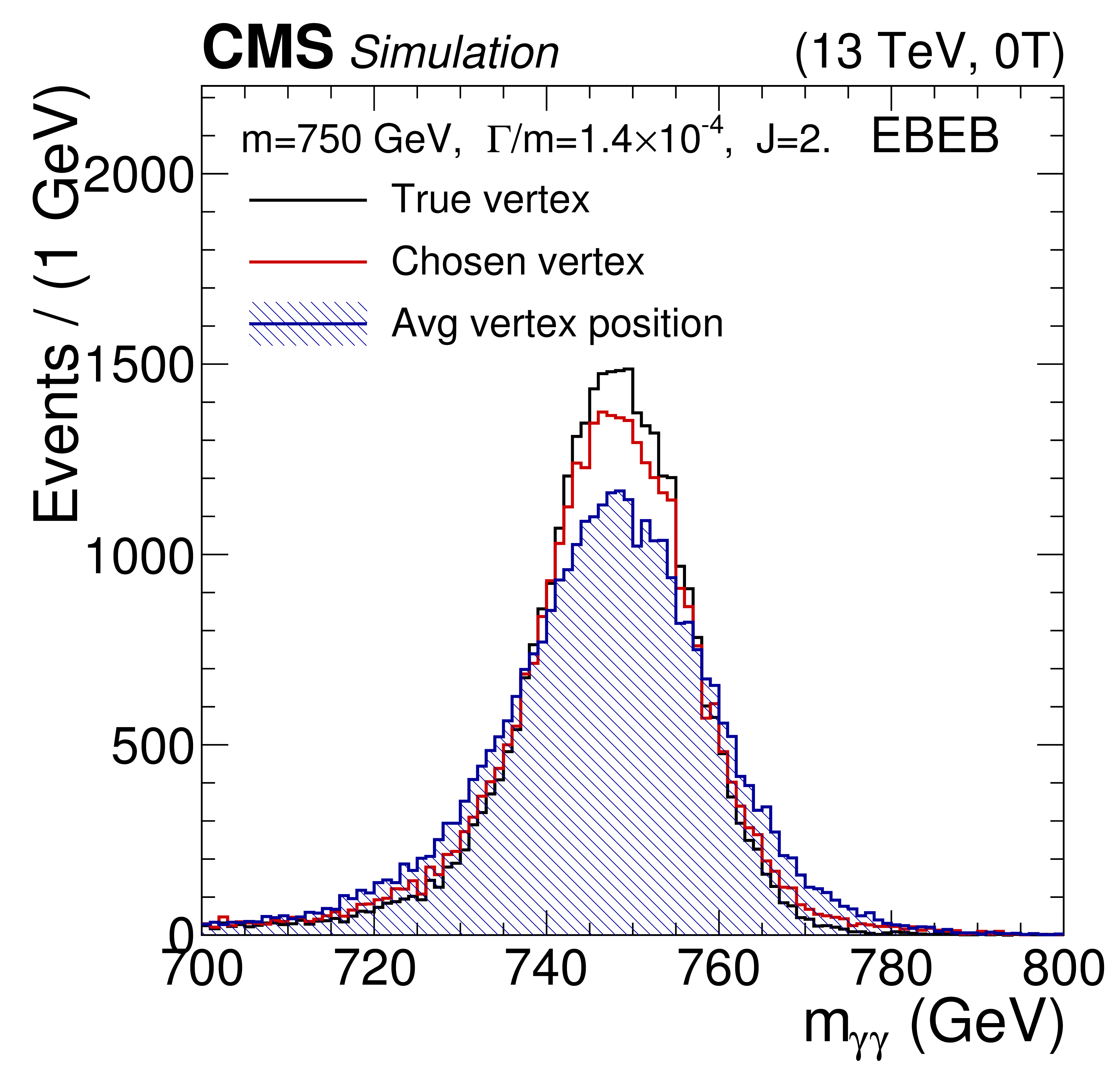
png pdf	Auxiliary Figure 1-a: Mass distribution for a narrow diphoton resonance in the B = 0 T analysis for difference choices of primary vertex. a: EBEB category, b: EBEE category.
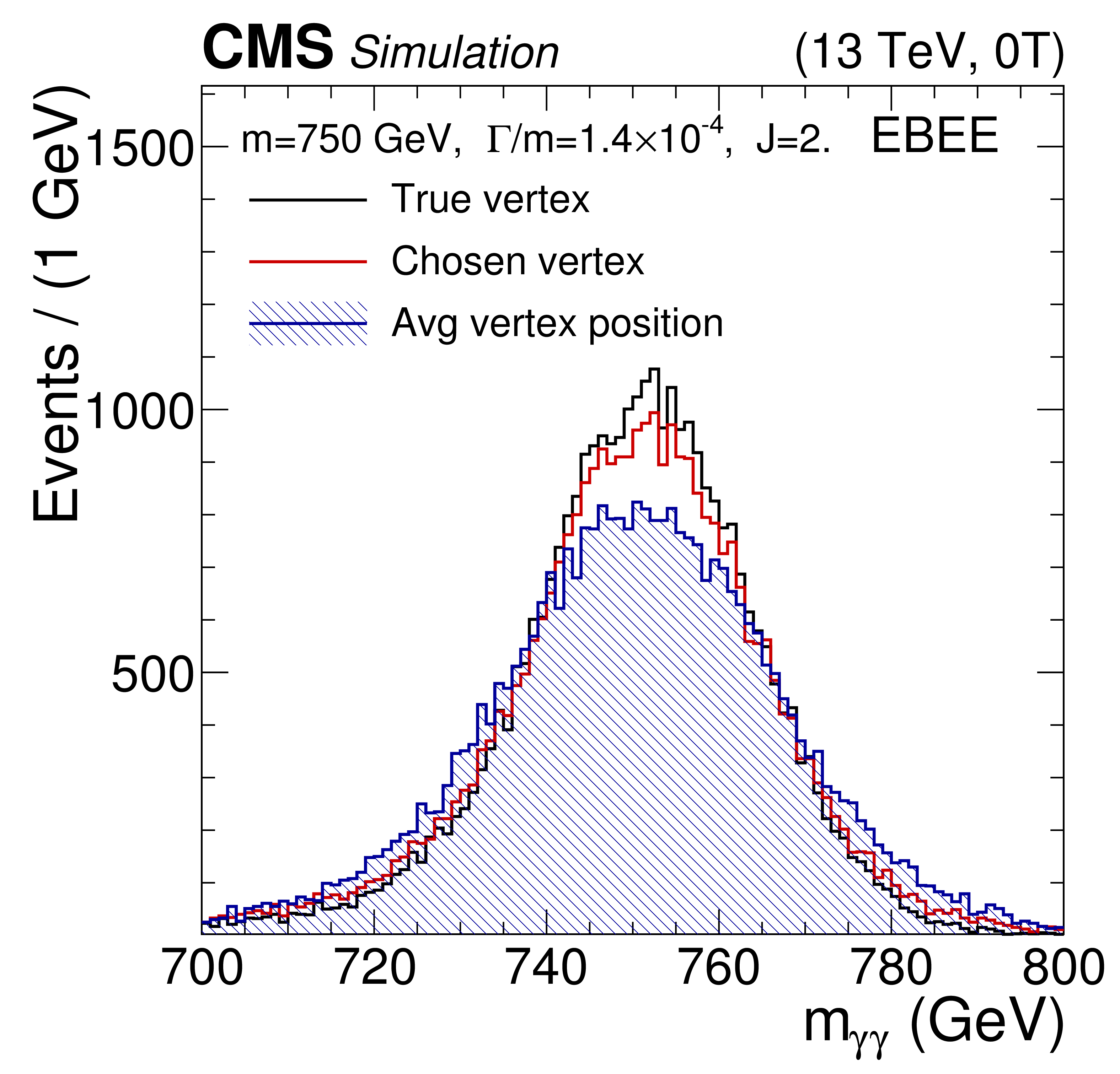
png pdf	Auxiliary Figure 1-b: Mass distribution for a narrow diphoton resonance in the B = 0 T analysis for difference choices of primary vertex. a: EBEB category, b: EBEE category.
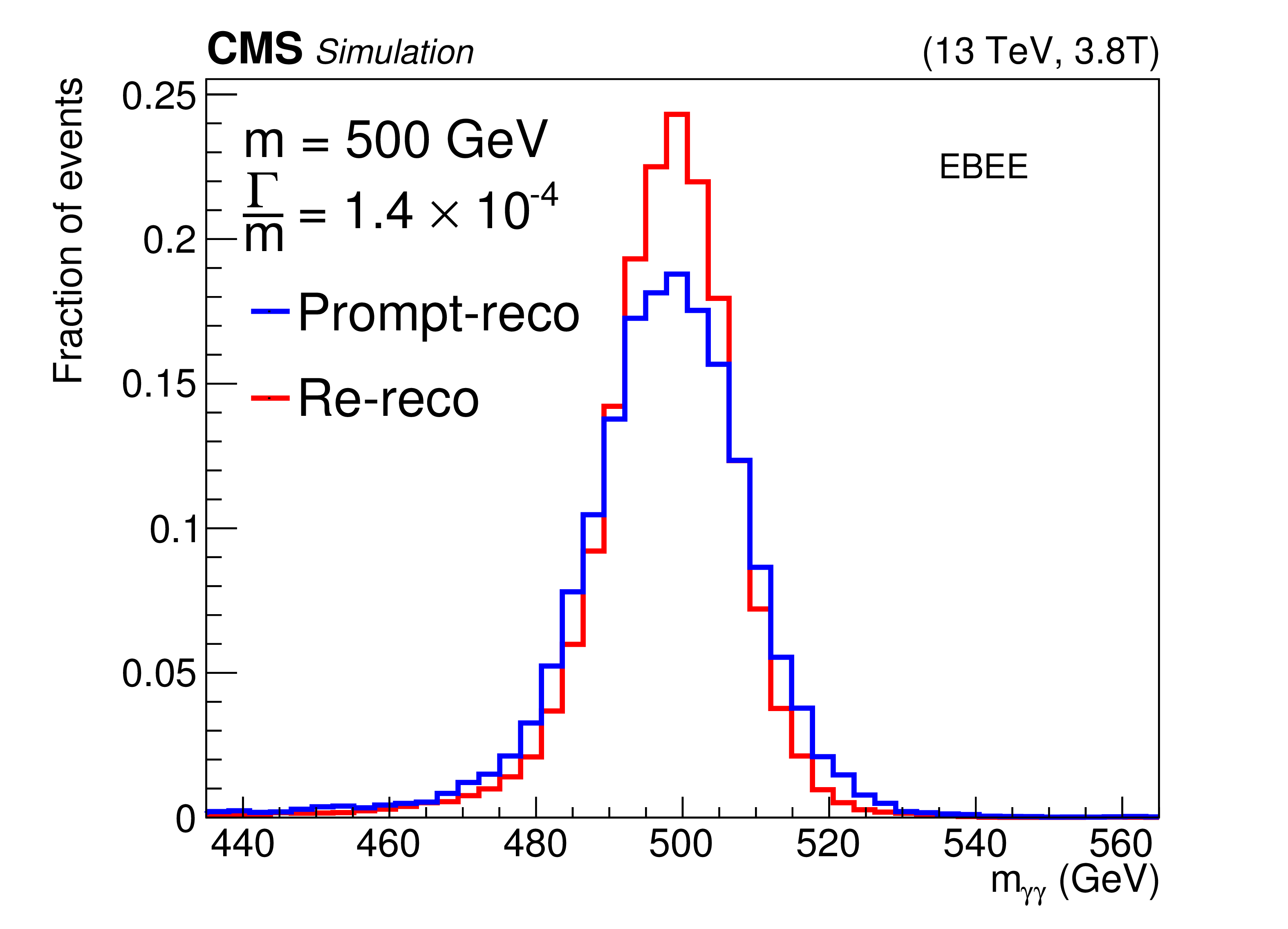
png pdf	Auxiliary Figure 2-a: Mass distribution for a narrow diphoton resonance in the B = 3.8 T analysis. The resolution obtained with the calibration used in Ref.[15] (``prompt-reco'') is compared to the one used in this analysis (``re-reco''). Left: EBEB category, right: EBEE category.
png pdf	Auxiliary Figure 2-b: Mass distribution for a narrow diphoton resonance in the B = 3.8 T analysis. The resolution obtained with the calibration used in Ref.[15] (``prompt-reco'') is compared to the one used in this analysis (``re-reco''). Left: EBEB category, right: EBEE category.
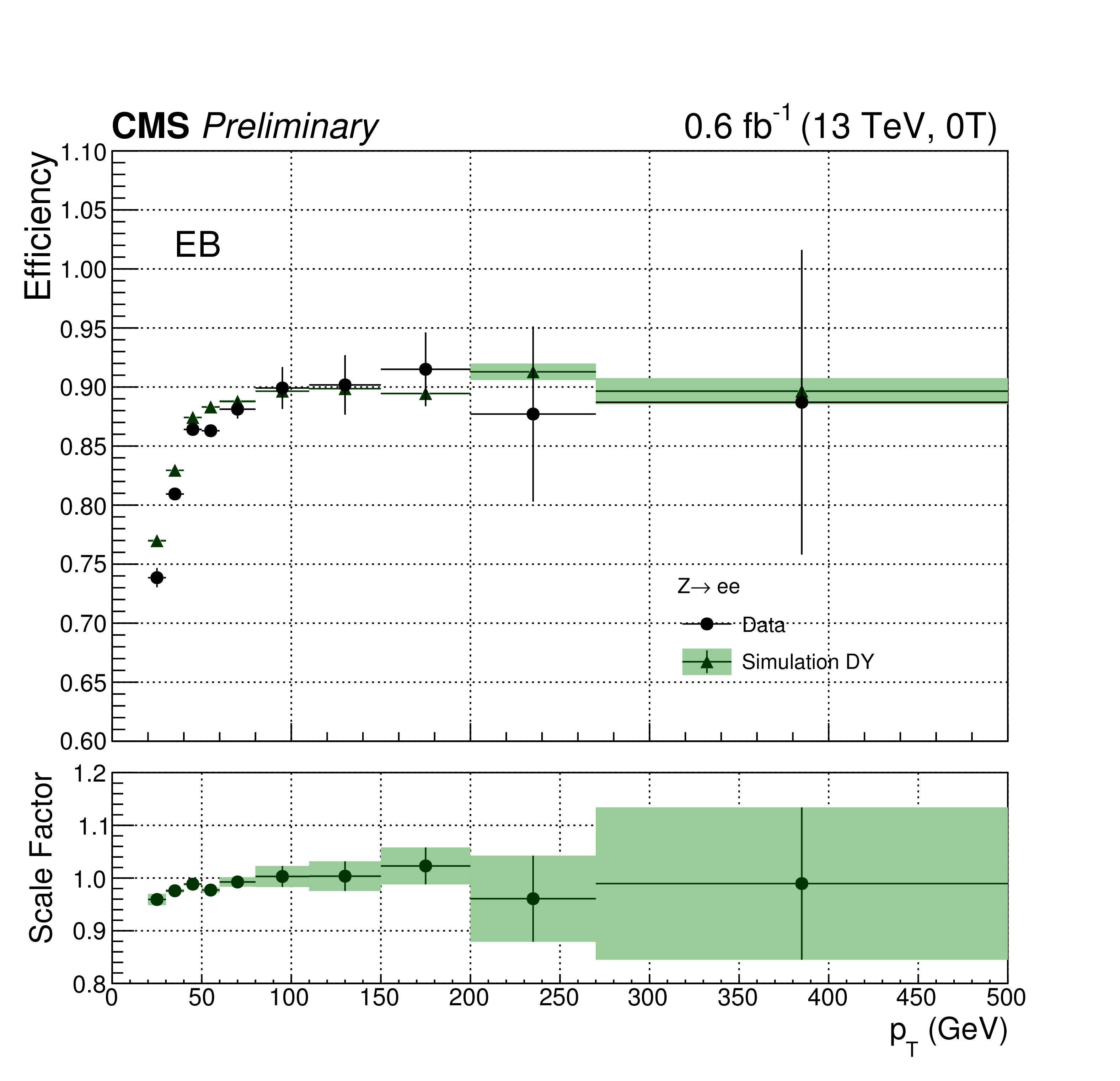
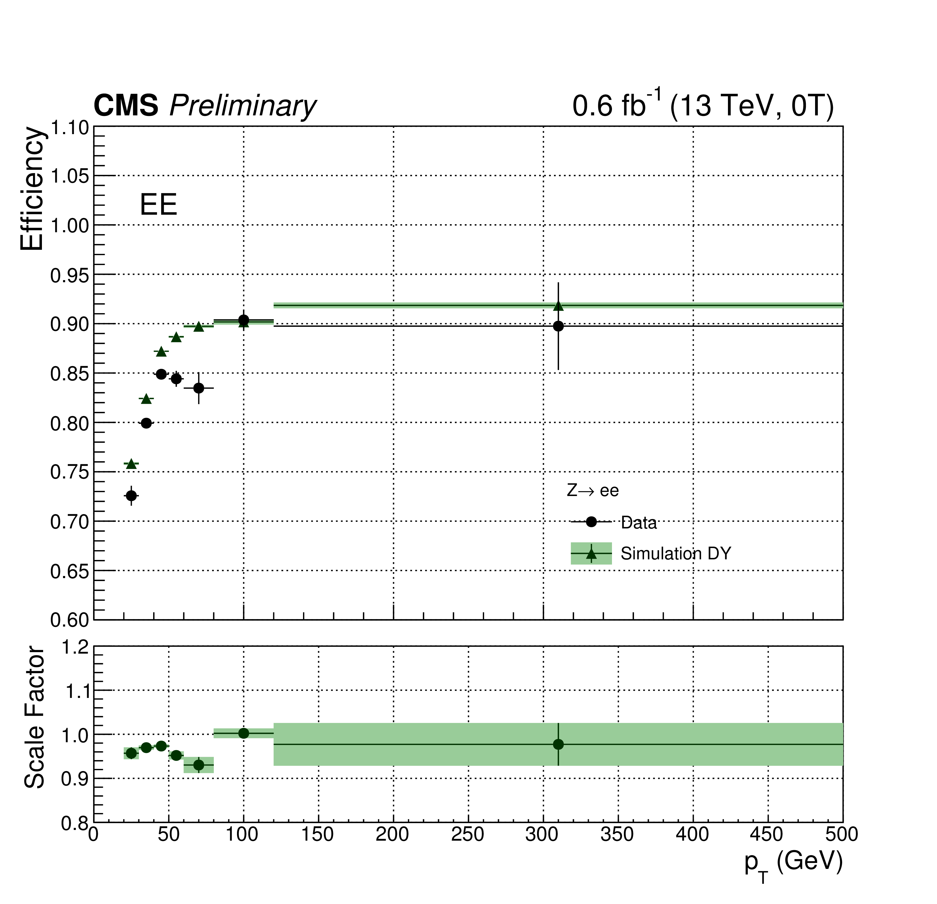
png pdf	Auxiliary Figure 3-a: Photon identification efficiency for all selection requirements except the electron rejection, measured in barrel (left) and end caps (right) using the tag and probe method for both data and simulated events in the B = 0 T dataset. Bottom: ratio of efficiencies found in data and simulated events.
png pdf	Auxiliary Figure 3-b: Photon identification efficiency for all selection requirements except the electron rejection, measured in barrel (left) and end caps (right) using the tag and probe method for both data and simulated events in the B = 0 T dataset. Bottom: ratio of efficiencies found in data and simulated events.
png pdf	Auxiliary Figure 4-a: Observed background only p-values obtained on the 13 TeV dataset. The mass range 500 GeV $< {m} <$ 850 GeV is shown is for resonances of ${\Gamma / m} = 1.4\times 10^{-4}$ and $5.6\times 10^{-2}$ . The contributions of the B = 3.8 T and B = 0 T datasets are shown separately. Due to the different size of the two datasets, the weight of the B = 0 T categories in the combined result is, at ${m} =$ 760 GeV, roughly one half of that of the B = 3.8 T ones. The a,c (b,d) column corresponds to the scalar (RS graviton) signals.
png pdf	Auxiliary Figure 4-b: Observed background only p-values obtained on the 13 TeV dataset. The mass range 500 GeV $< {m} <$ 850 GeV is shown is for resonances of ${\Gamma / m} = 1.4\times 10^{-4}$ and $5.6\times 10^{-2}$ . The contributions of the B = 3.8 T and B = 0 T datasets are shown separately. Due to the different size of the two datasets, the weight of the B = 0 T categories in the combined result is, at ${m} =$ 760 GeV, roughly one half of that of the B = 3.8 T ones. The a,c (b,d) column corresponds to the scalar (RS graviton) signals.
png pdf	Auxiliary Figure 4-c: Observed background only p-values obtained on the 13 TeV dataset. The mass range 500 GeV $< {m} <$ 850 GeV is shown is for resonances of ${\Gamma / m} = 1.4\times 10^{-4}$ and $5.6\times 10^{-2}$ . The contributions of the B = 3.8 T and B = 0 T datasets are shown separately. Due to the different size of the two datasets, the weight of the B = 0 T categories in the combined result is, at ${m} =$ 760 GeV, roughly one half of that of the B = 3.8 T ones. The a,c (b,d) column corresponds to the scalar (RS graviton) signals.
png pdf	Auxiliary Figure 4-d: Observed background only p-values obtained on the 13 TeV dataset. The mass range 500 GeV $< {m} <$ 850 GeV is shown is for resonances of ${\Gamma / m} = 1.4\times 10^{-4}$ and $5.6\times 10^{-2}$ . The contributions of the B = 3.8 T and B = 0 T datasets are shown separately. Due to the different size of the two datasets, the weight of the B = 0 T categories in the combined result is, at ${m} =$ 760 GeV, roughly one half of that of the B = 3.8 T ones. The a,c (b,d) column corresponds to the scalar (RS graviton) signals.
png pdf	Auxiliary Figure 5-a: Observed background only p-values obtained from the combination of 8 TeV and 13 TeV results for different signal hypotheses in the mass range 500 GeV $< {m} <$ 850 GeV. The contributions of the 8 and 13 TeV datasets are shown separately. At ${m} =$ 750 GeV, the two datasets contribute with similar weights to the combined result. The a,c,e (b,d,f) column corresponds to the scalar (RS graviton) signals.
png pdf	Auxiliary Figure 5-b: Observed background only p-values obtained from the combination of 8 TeV and 13 TeV results for different signal hypotheses in the mass range 500 GeV $< {m} <$ 850 GeV. The contributions of the 8 and 13 TeV datasets are shown separately. At ${m} =$ 750 GeV, the two datasets contribute with similar weights to the combined result. The a,c,e (b,d,f) column corresponds to the scalar (RS graviton) signals.
png pdf	Auxiliary Figure 5-c: Observed background only p-values obtained from the combination of 8 TeV and 13 TeV results for different signal hypotheses in the mass range 500 GeV $< {m} <$ 850 GeV. The contributions of the 8 and 13 TeV datasets are shown separately. At ${m} =$ 750 GeV, the two datasets contribute with similar weights to the combined result. The a,c,e (b,d,f) column corresponds to the scalar (RS graviton) signals.
png pdf	Auxiliary Figure 5-d: Observed background only p-values obtained from the combination of 8 TeV and 13 TeV results for different signal hypotheses in the mass range 500 GeV $< {m} <$ 850 GeV. The contributions of the 8 and 13 TeV datasets are shown separately. At ${m} =$ 750 GeV, the two datasets contribute with similar weights to the combined result. The a,c,e (b,d,f) column corresponds to the scalar (RS graviton) signals.
png pdf	Auxiliary Figure 5-e: Observed background only p-values obtained from the combination of 8 TeV and 13 TeV results for different signal hypotheses in the mass range 500 GeV $< {m} <$ 850 GeV. The contributions of the 8 and 13 TeV datasets are shown separately. At ${m} =$ 750 GeV, the two datasets contribute with similar weights to the combined result. The a,c,e (b,d,f) column corresponds to the scalar (RS graviton) signals.
png pdf	Auxiliary Figure 5-f: Observed background only p-values obtained from the combination of 8 TeV and 13 TeV results for different signal hypotheses in the mass range 500 GeV $< {m} <$ 850 GeV. The contributions of the 8 and 13 TeV datasets are shown separately. At ${m} =$ 750 GeV, the two datasets contribute with similar weights to the combined result. The a,c,e (b,d,f) column corresponds to the scalar (RS graviton) signals.
png pdf	Auxiliary Figure 6-a: Expected and observed 95\% C.L. exclusion limits for different signal hypotheses for the B = 3.8 T dataset at 13 TeV. The range 500 GeV $< m <$ 4.5 TeV is shown for ${\Gamma / m} = 1.4\times 10^{-4}, 1.4\times 10^{-2}, 5.6\times 10^{-2}$ . The a,c,e (b,d,f) column corresponds to the scalar (RS graviton) signals.
png pdf	Auxiliary Figure 6-b: Expected and observed 95\% C.L. exclusion limits for different signal hypotheses for the B = 3.8 T dataset at 13 TeV. The range 500 GeV $< m <$ 4.5 TeV is shown for ${\Gamma / m} = 1.4\times 10^{-4}, 1.4\times 10^{-2}, 5.6\times 10^{-2}$ . The a,c,e (b,d,f) column corresponds to the scalar (RS graviton) signals.
png pdf	Auxiliary Figure 6-c: Expected and observed 95\% C.L. exclusion limits for different signal hypotheses for the B = 3.8 T dataset at 13 TeV. The range 500 GeV $< m <$ 4.5 TeV is shown for ${\Gamma / m} = 1.4\times 10^{-4}, 1.4\times 10^{-2}, 5.6\times 10^{-2}$ . The a,c,e (b,d,f) column corresponds to the scalar (RS graviton) signals.
png pdf	Auxiliary Figure 6-d: Expected and observed 95\% C.L. exclusion limits for different signal hypotheses for the B = 3.8 T dataset at 13 TeV. The range 500 GeV $< m <$ 4.5 TeV is shown for ${\Gamma / m} = 1.4\times 10^{-4}, 1.4\times 10^{-2}, 5.6\times 10^{-2}$ . The a,c,e (b,d,f) column corresponds to the scalar (RS graviton) signals.
png pdf	Auxiliary Figure 6-e: Expected and observed 95\% C.L. exclusion limits for different signal hypotheses for the B = 3.8 T dataset at 13 TeV. The range 500 GeV $< m <$ 4.5 TeV is shown for ${\Gamma / m} = 1.4\times 10^{-4}, 1.4\times 10^{-2}, 5.6\times 10^{-2}$ . The a,c,e (b,d,f) column corresponds to the scalar (RS graviton) signals.
png pdf	Auxiliary Figure 6-f: Expected and observed 95\% C.L. exclusion limits for different signal hypotheses for the B = 3.8 T dataset at 13 TeV. The range 500 GeV $< m <$ 4.5 TeV is shown for ${\Gamma / m} = 1.4\times 10^{-4}, 1.4\times 10^{-2}, 5.6\times 10^{-2}$ . The a,c,e (b,d,f) column corresponds to the scalar (RS graviton) signals.
png pdf	Auxiliary Figure 7-a: Expected and observed 95\% C.L. exclusion limits for different signal hypotheses for the B = 0 T dataset at 13 TeV. The range 500 GeV $< m <$ 4.5 TeV is shown for ${\Gamma / m} = 1.4\times 10^{-4}, 1.4\times 10^{-2}, 5.6\times 10^{-2}$ . The a,c,e (b,d,f) column corresponds to the scalar (RS graviton) signals.
png pdf	Auxiliary Figure 7-b: Expected and observed 95\% C.L. exclusion limits for different signal hypotheses for the B = 0 T dataset at 13 TeV. The range 500 GeV $< m <$ 4.5 TeV is shown for ${\Gamma / m} = 1.4\times 10^{-4}, 1.4\times 10^{-2}, 5.6\times 10^{-2}$ . The a,c,e (b,d,f) column corresponds to the scalar (RS graviton) signals.
png pdf	Auxiliary Figure 7-c: Expected and observed 95\% C.L. exclusion limits for different signal hypotheses for the B = 0 T dataset at 13 TeV. The range 500 GeV $< m <$ 4.5 TeV is shown for ${\Gamma / m} = 1.4\times 10^{-4}, 1.4\times 10^{-2}, 5.6\times 10^{-2}$ . The a,c,e (b,d,f) column corresponds to the scalar (RS graviton) signals.
png pdf	Auxiliary Figure 7-d: Expected and observed 95\% C.L. exclusion limits for different signal hypotheses for the B = 0 T dataset at 13 TeV. The range 500 GeV $< m <$ 4.5 TeV is shown for ${\Gamma / m} = 1.4\times 10^{-4}, 1.4\times 10^{-2}, 5.6\times 10^{-2}$ . The a,c,e (b,d,f) column corresponds to the scalar (RS graviton) signals.
png pdf	Auxiliary Figure 7-e: Expected and observed 95\% C.L. exclusion limits for different signal hypotheses for the B = 0 T dataset at 13 TeV. The range 500 GeV $< m <$ 4.5 TeV is shown for ${\Gamma / m} = 1.4\times 10^{-4}, 1.4\times 10^{-2}, 5.6\times 10^{-2}$ . The a,c,e (b,d,f) column corresponds to the scalar (RS graviton) signals.
png pdf	Auxiliary Figure 7-f: Expected and observed 95\% C.L. exclusion limits for different signal hypotheses for the B = 0 T dataset at 13 TeV. The range 500 GeV $< m <$ 4.5 TeV is shown for ${\Gamma / m} = 1.4\times 10^{-4}, 1.4\times 10^{-2}, 5.6\times 10^{-2}$ . The a,c,e (b,d,f) column corresponds to the scalar (RS graviton) signals.

Compact Muon Solenoid
LHC, CERN