

Compact Muon Solenoid
LHC, CERN
| CMS-PAS-EXO-12-055 | ||
| Search for New Physics in the V-jet + MET final state | ||
| CMS Collaboration | ||
| July 2015 [revised: October 2015] | ||
| Abstract: A search is presented for an excess of events with a high energy jet in association with a large missing transverse momentum in a data sample of proton-proton interactions at centre-of-mass energy of 8TeV. The data correspond to an integrated luminosity of 19.7 fb$^{-1}$ collected by the CMS detector at the LHC. Additional sensitivity is achieved by tagging events consistent with the jet originating from a hadronically decaying vector boson. Limits are obtained on the branching ratio of a standard model Higgs boson decaying invisibly. The search is also interpreted in terms of dark matter production to place constraints on the parameter space of simplified models. | ||
|
Links:
CDS record (PDF) ;
CADI line (restricted) ; Figures are also available from the CDS record. These preliminary results are superseded in this paper, JHEP 12 (2016) 083 [Erratum: JHEP 08 (2017) 035]. The superseded preliminary plots can be found here. |
||
| Figures | |

png ; pdf |
Figure 1-a:
Diagrams for the monojet (a) and mono-V (b) processes with a spin-1 mediator. |

png ; pdf |
Figure 1-b:
Diagrams for the monojet (a) and mono-V (b) processes with a spin-1 mediator. |

png ; pdf |
Figure 2-a:
Diagrams for production of the monojet (a) and mono-V signature through Higgs-strahlung (b), through a scalar mediator. |

png ; pdf |
Figure 2-b:
Diagrams for production of the monojet (a) and mono-V signature through Higgs-strahlung (b), through a scalar mediator. |
png ; pdf |
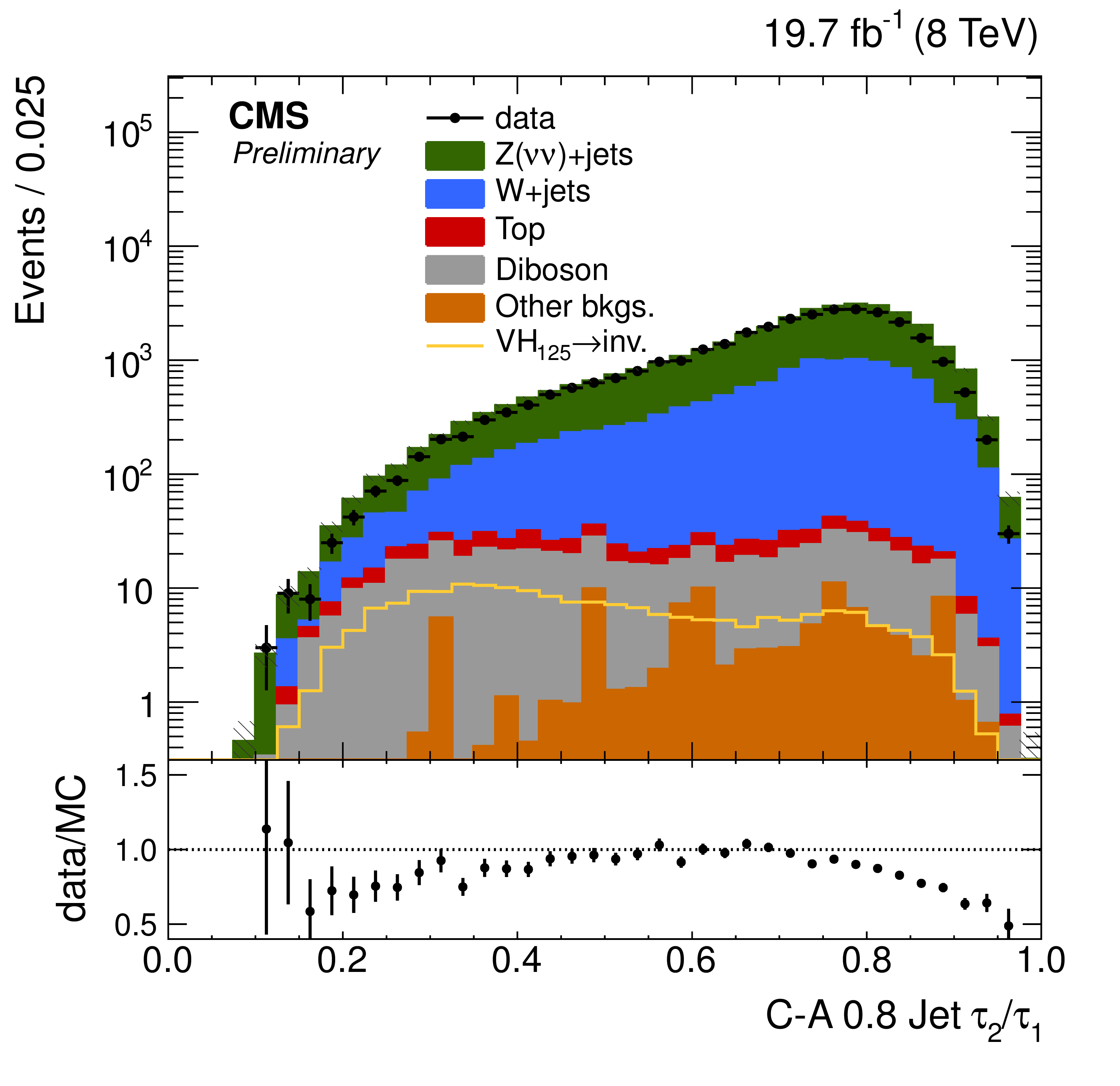
Figure 3-a:
Distributions of $\tau _2/\tau _1$ before the jet mass cut (a) and pruned jet mass (b) for events in data and MC in the boosted event category. A cut of $\tau _2/\tau _1<$ 0.5 is applied in figure b. |

png ; pdf |
Figure 3-b:
Distributions of $\tau _2/\tau _1$ before the jet mass cut (a) and pruned jet mass (b) for events in data and MC in the boosted event category. A cut of $\tau _2/\tau _1<$ 0.5 is applied in figure b. |
png ; pdf |
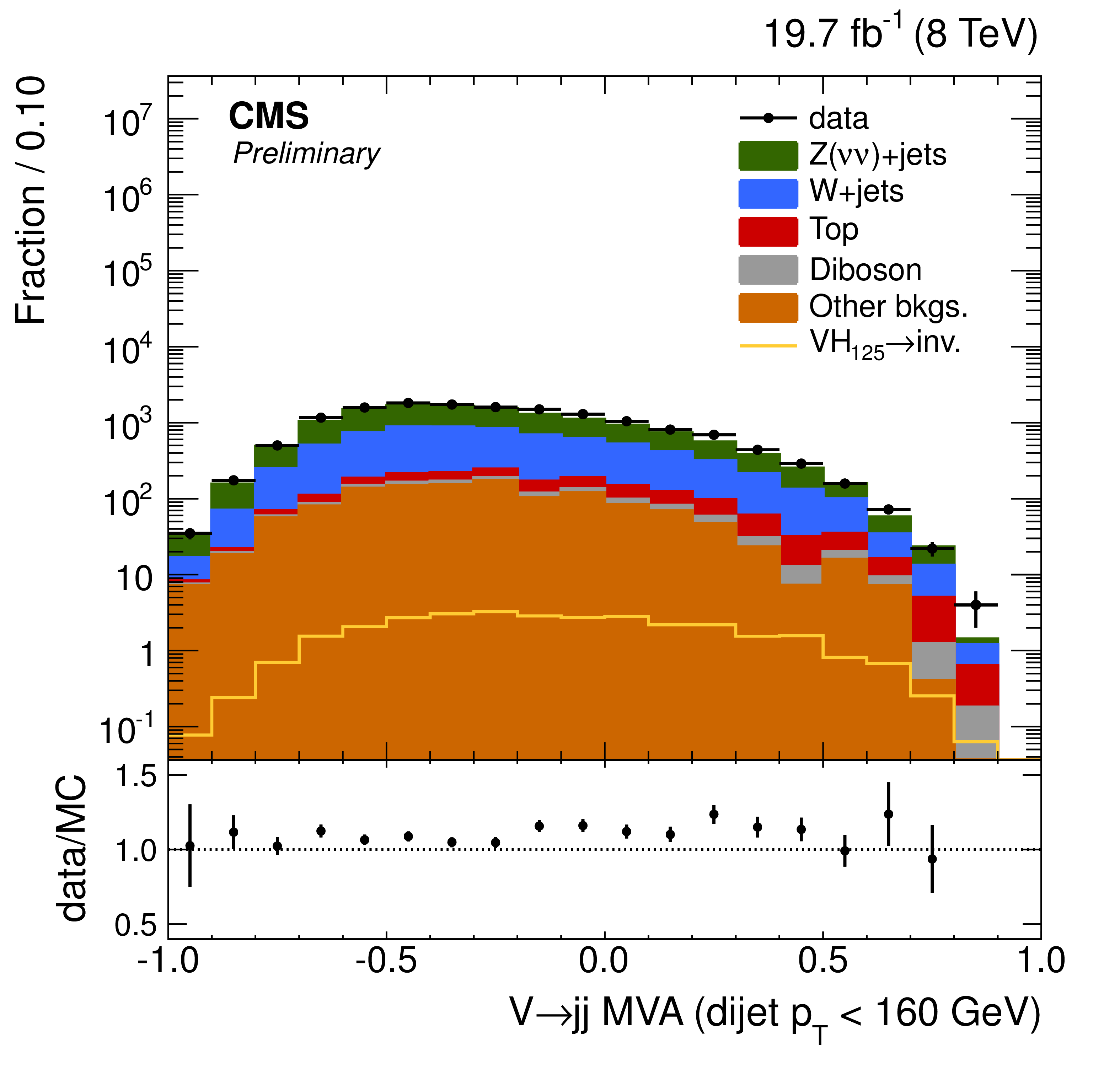
Figure 4-a:
Resolved V-tagger variable distribution in simulation and data after all other signal region cuts in the resolved category. The distributions are shown split into dijet $ {p_{\mathrm {T}}} <$ 160 GeV (a) and dijet $ {p_{\mathrm {T}}} >$ 160 GeV (b), corresponding roughly to the point at which jets begin to overlap. The expected distribution for the vector boson produced in association with a Higgs boson with a mass of 125 GeV is shown. |

png ; pdf |
Figure 4-b:
Resolved V-tagger variable distribution in simulation and data after all other signal region cuts in the resolved category. The distributions are shown split into dijet $ {p_{\mathrm {T}}} <$ 160 GeV (a) and dijet $ {p_{\mathrm {T}}} >$ 160 GeV (b), corresponding roughly to the point at which jets begin to overlap. The expected distribution for the vector boson produced in association with a Higgs boson with a mass of 125 GeV is shown. |
png ; pdf |
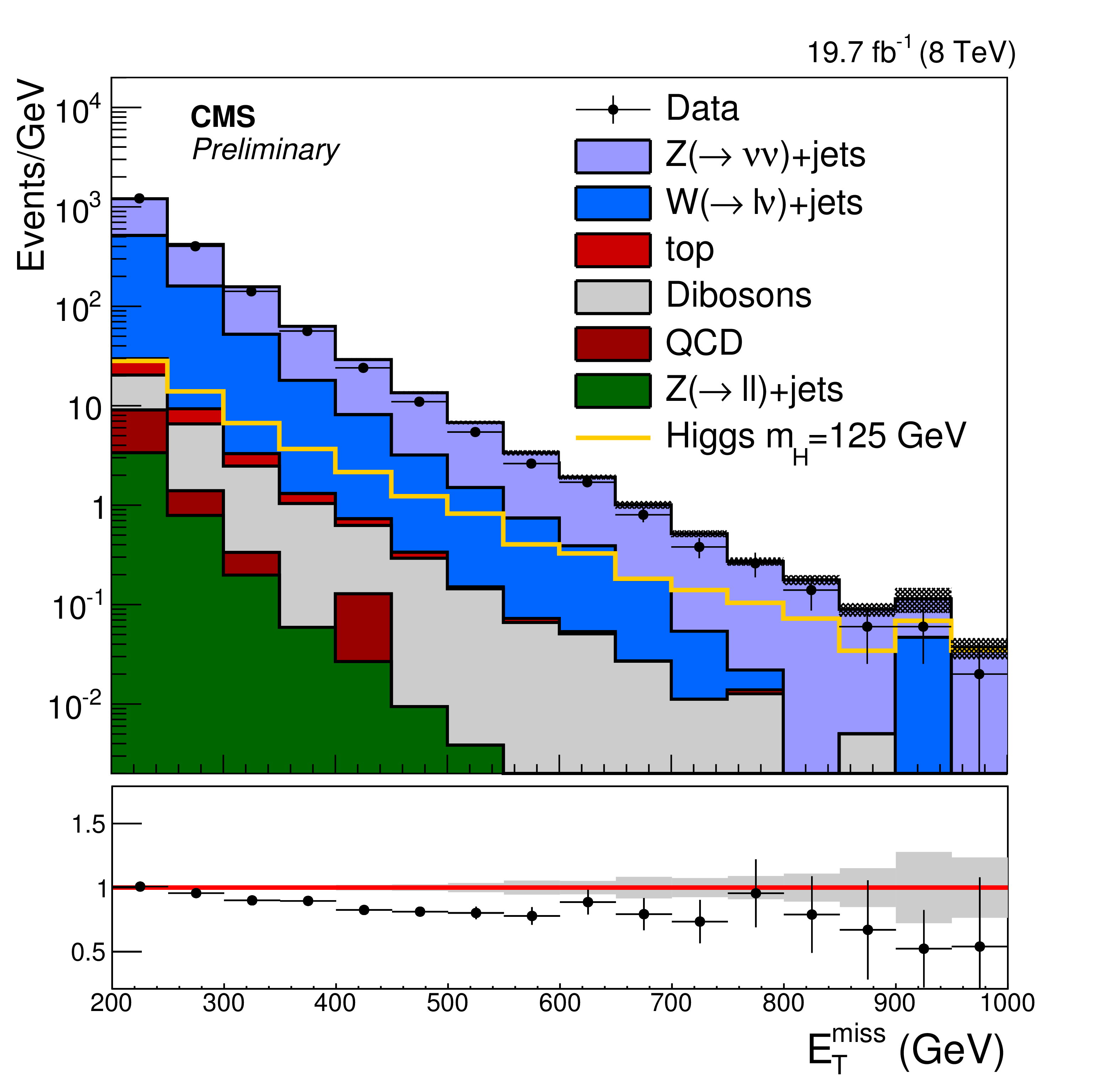
Figure 5-a:
Distributions of $ {E_{\mathrm {T}}^{\text {miss}}} $ (a) and leading jet $p_{\mathrm{T}}$ (b) in simulated events and data after the signal selection for all three event categories combined. The expected distribution for a Higgs boson with mass 125 GeV is shown assuming the SM Higgs cross-section and an invisible branching ratio of 100%. The gray band in the ratios indicate the statistical uncertainty from the limited number of background MC events. |
png ; pdf |
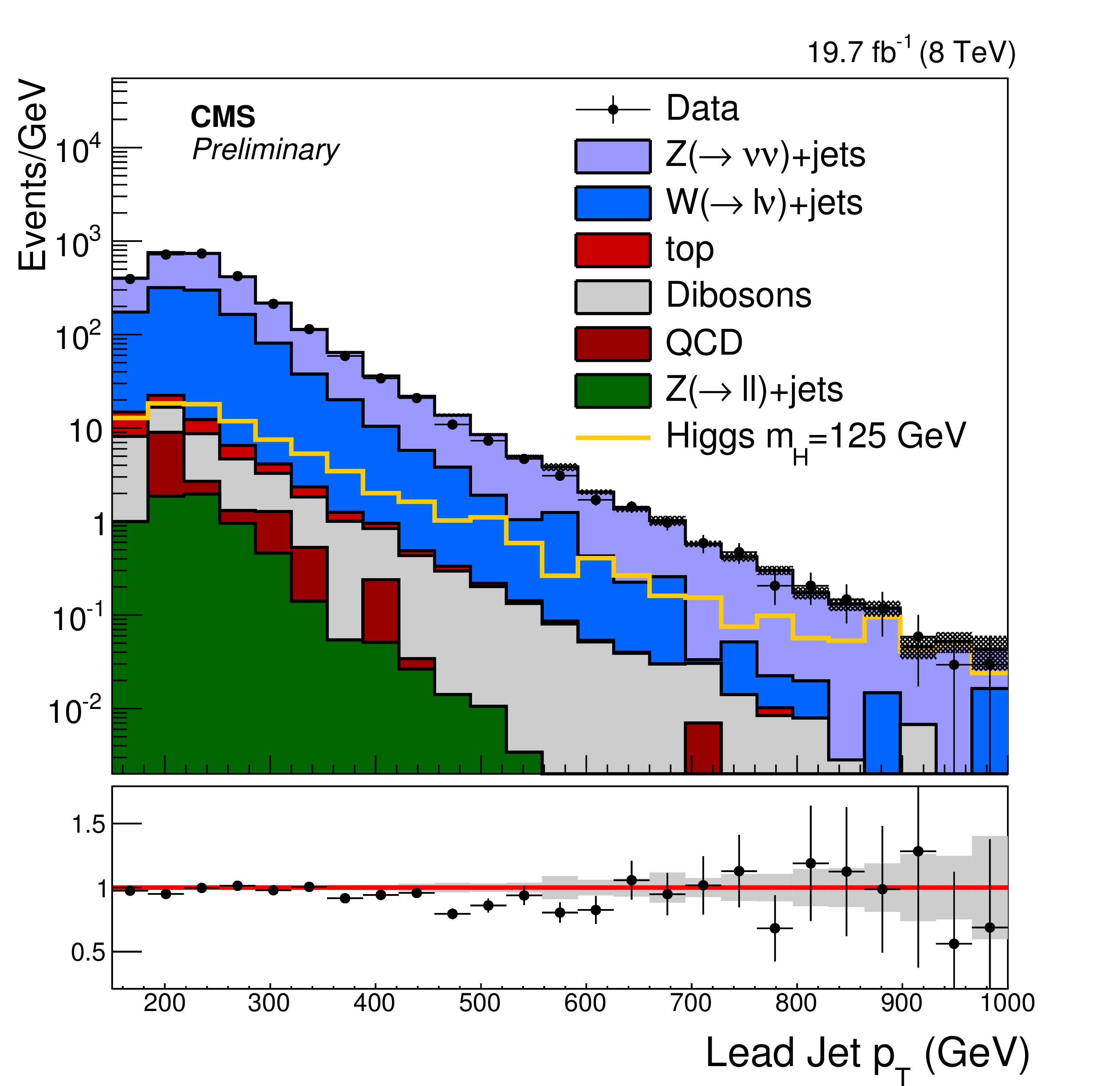
Figure 5-b:
Distributions of $ {E_{\mathrm {T}}^{\text {miss}}} $ (a) and leading jet $p_{\mathrm{T}}$ (b) in simulated events and data after the signal selection for all three event categories combined. The expected distribution for a Higgs boson with mass 125 GeV is shown assuming the SM Higgs cross-section and an invisible branching ratio of 100%. The gray band in the ratios indicate the statistical uncertainty from the limited number of background MC events. |
png ; pdf |
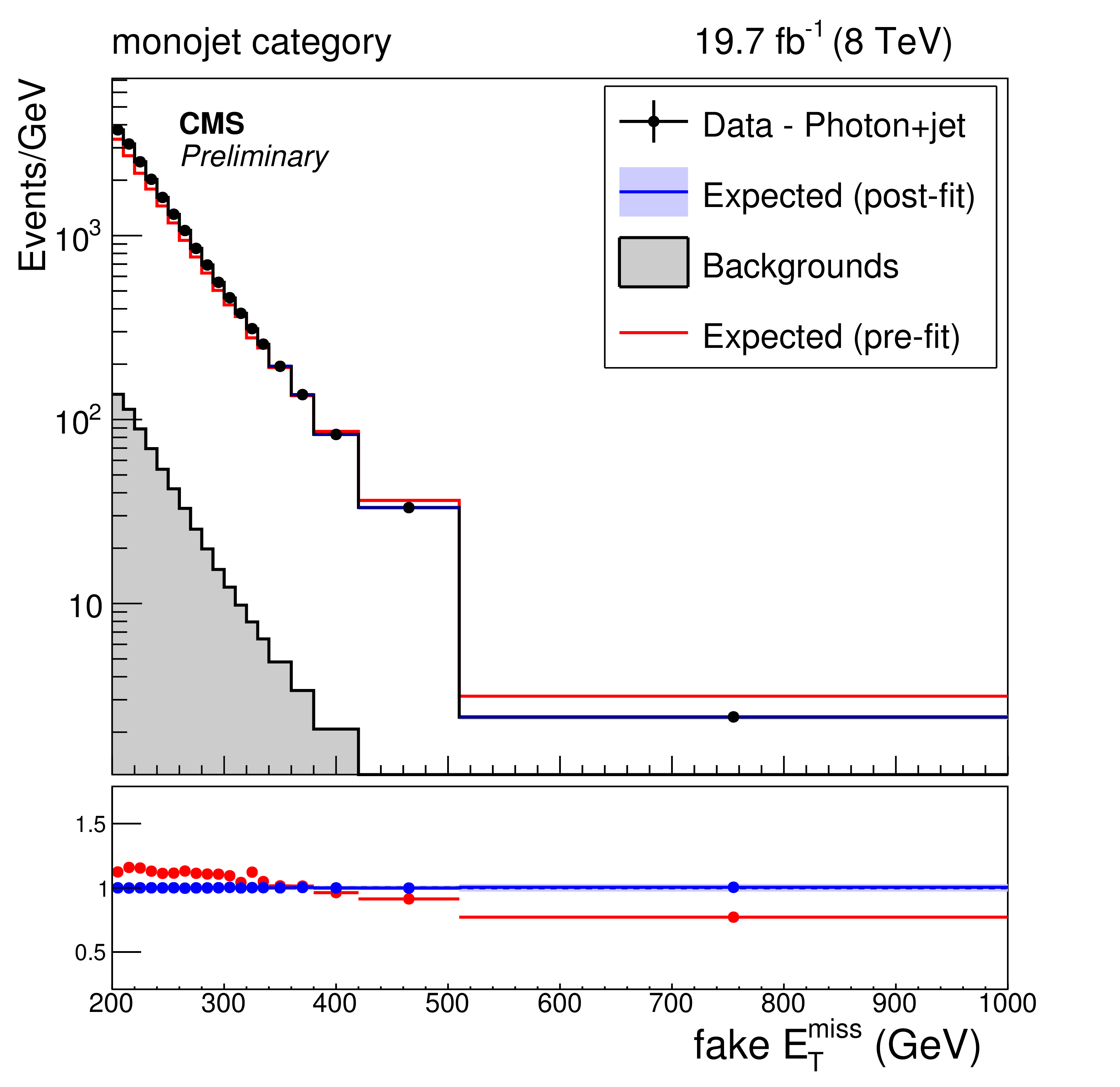
Figure 6-a:
Expected and observed fake $ {E_{\mathrm {T}}^{\text {miss}}} $ distributions in the photon(a,d,g), dimuon (b,e,h) and single-muon(c,f,i) control regions after performing the simultaneous likelihood fit to the control regions. Each series of plot, (a,b,c), (d,e,f) and (g,h,i), shows the result of the fit in the monojet, resolved and boosted event categories respectively. The red line represents the expected distribution before fitting to the control regions, while the blue line shows the expectation after the fit. In the ratio, the blue and red points show the ratio of the observed data to the post-fit and pre-fit expectations respectively. The blue bands indicate the statistical and systematic uncertainties from the fit. |

png ; pdf |
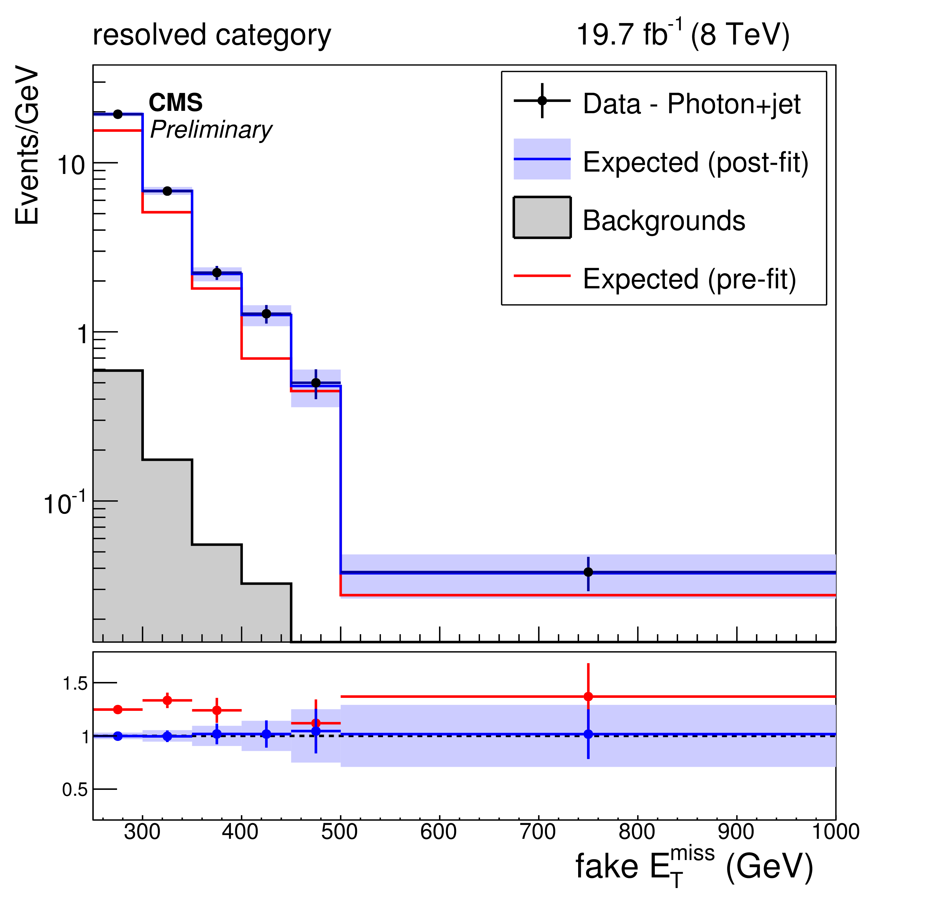
Figure 6-b:
Expected and observed fake $ {E_{\mathrm {T}}^{\text {miss}}} $ distributions in the photon(a,d,g), dimuon (b,e,h) and single-muon(c,f,i) control regions after performing the simultaneous likelihood fit to the control regions. Each series of plot, (a,b,c), (d,e,f) and (g,h,i), shows the result of the fit in the monojet, resolved and boosted event categories respectively. The red line represents the expected distribution before fitting to the control regions, while the blue line shows the expectation after the fit. In the ratio, the blue and red points show the ratio of the observed data to the post-fit and pre-fit expectations respectively. The blue bands indicate the statistical and systematic uncertainties from the fit. |

png ; pdf |
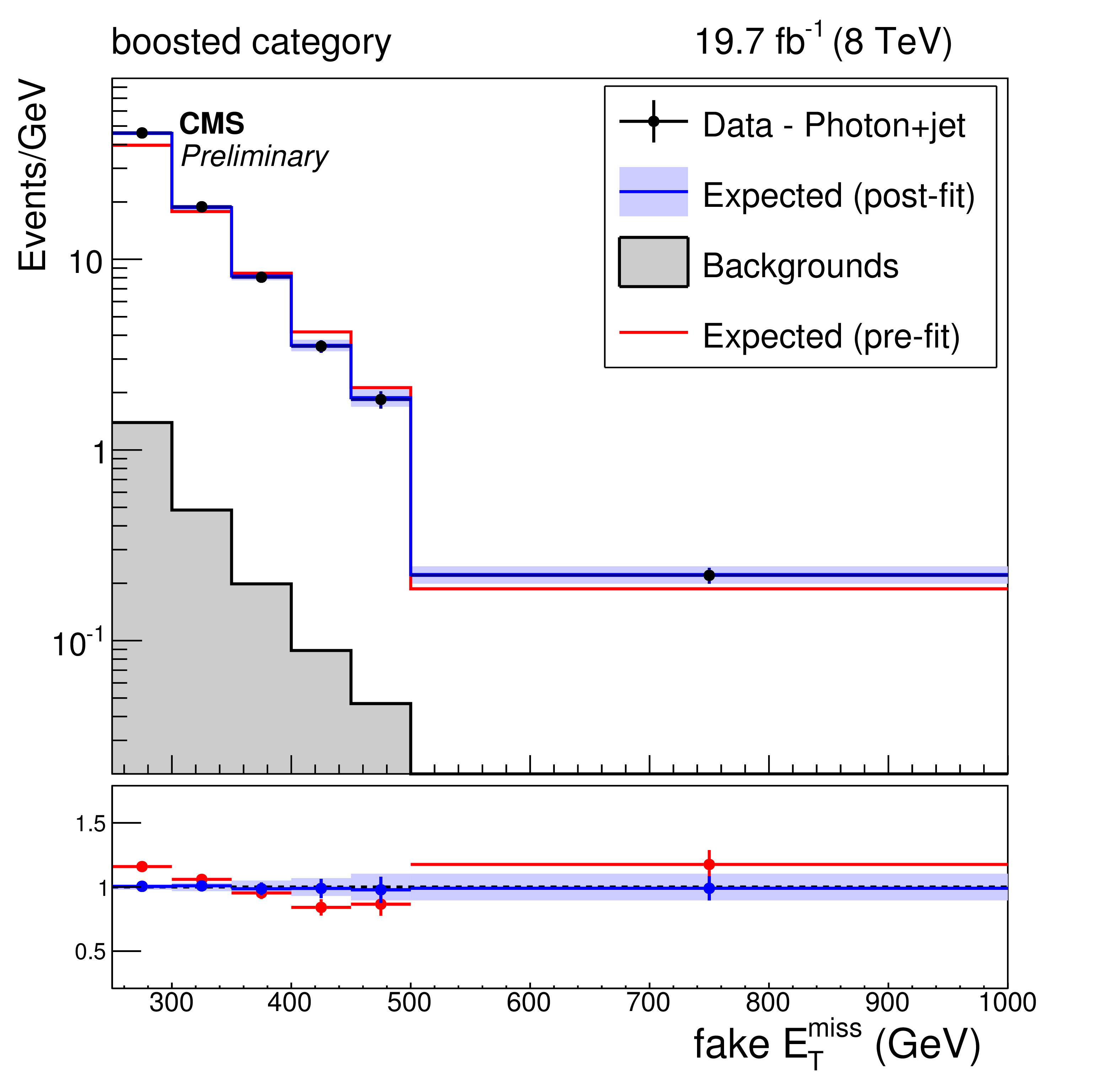
Figure 6-c:
Expected and observed fake $ {E_{\mathrm {T}}^{\text {miss}}} $ distributions in the photon(a,d,g), dimuon (b,e,h) and single-muon(c,f,i) control regions after performing the simultaneous likelihood fit to the control regions. Each series of plot, (a,b,c), (d,e,f) and (g,h,i), shows the result of the fit in the monojet, resolved and boosted event categories respectively. The red line represents the expected distribution before fitting to the control regions, while the blue line shows the expectation after the fit. In the ratio, the blue and red points show the ratio of the observed data to the post-fit and pre-fit expectations respectively. The blue bands indicate the statistical and systematic uncertainties from the fit. |
png ; pdf |
Figure 6-d:
Expected and observed fake $ {E_{\mathrm {T}}^{\text {miss}}} $ distributions in the photon(a,d,g), dimuon (b,e,h) and single-muon(c,f,i) control regions after performing the simultaneous likelihood fit to the control regions. Each series of plot, (a,b,c), (d,e,f) and (g,h,i), shows the result of the fit in the monojet, resolved and boosted event categories respectively. The red line represents the expected distribution before fitting to the control regions, while the blue line shows the expectation after the fit. In the ratio, the blue and red points show the ratio of the observed data to the post-fit and pre-fit expectations respectively. The blue bands indicate the statistical and systematic uncertainties from the fit. |

png ; pdf |
Figure 6-e:
Expected and observed fake $ {E_{\mathrm {T}}^{\text {miss}}} $ distributions in the photon(a,d,g), dimuon (b,e,h) and single-muon(c,f,i) control regions after performing the simultaneous likelihood fit to the control regions. Each series of plot, (a,b,c), (d,e,f) and (g,h,i), shows the result of the fit in the monojet, resolved and boosted event categories respectively. The red line represents the expected distribution before fitting to the control regions, while the blue line shows the expectation after the fit. In the ratio, the blue and red points show the ratio of the observed data to the post-fit and pre-fit expectations respectively. The blue bands indicate the statistical and systematic uncertainties from the fit. |

png ; pdf |
Figure 6-f:
Expected and observed fake $ {E_{\mathrm {T}}^{\text {miss}}} $ distributions in the photon(a,d,g), dimuon (b,e,h) and single-muon(c,f,i) control regions after performing the simultaneous likelihood fit to the control regions. Each series of plot, (a,b,c), (d,e,f) and (g,h,i), shows the result of the fit in the monojet, resolved and boosted event categories respectively. The red line represents the expected distribution before fitting to the control regions, while the blue line shows the expectation after the fit. In the ratio, the blue and red points show the ratio of the observed data to the post-fit and pre-fit expectations respectively. The blue bands indicate the statistical and systematic uncertainties from the fit. |
png ; pdf |
Figure 6-g:
Expected and observed fake $ {E_{\mathrm {T}}^{\text {miss}}} $ distributions in the photon(a,d,g), dimuon (b,e,h) and single-muon(c,f,i) control regions after performing the simultaneous likelihood fit to the control regions. Each series of plot, (a,b,c), (d,e,f) and (g,h,i), shows the result of the fit in the monojet, resolved and boosted event categories respectively. The red line represents the expected distribution before fitting to the control regions, while the blue line shows the expectation after the fit. In the ratio, the blue and red points show the ratio of the observed data to the post-fit and pre-fit expectations respectively. The blue bands indicate the statistical and systematic uncertainties from the fit. |
png ; pdf |
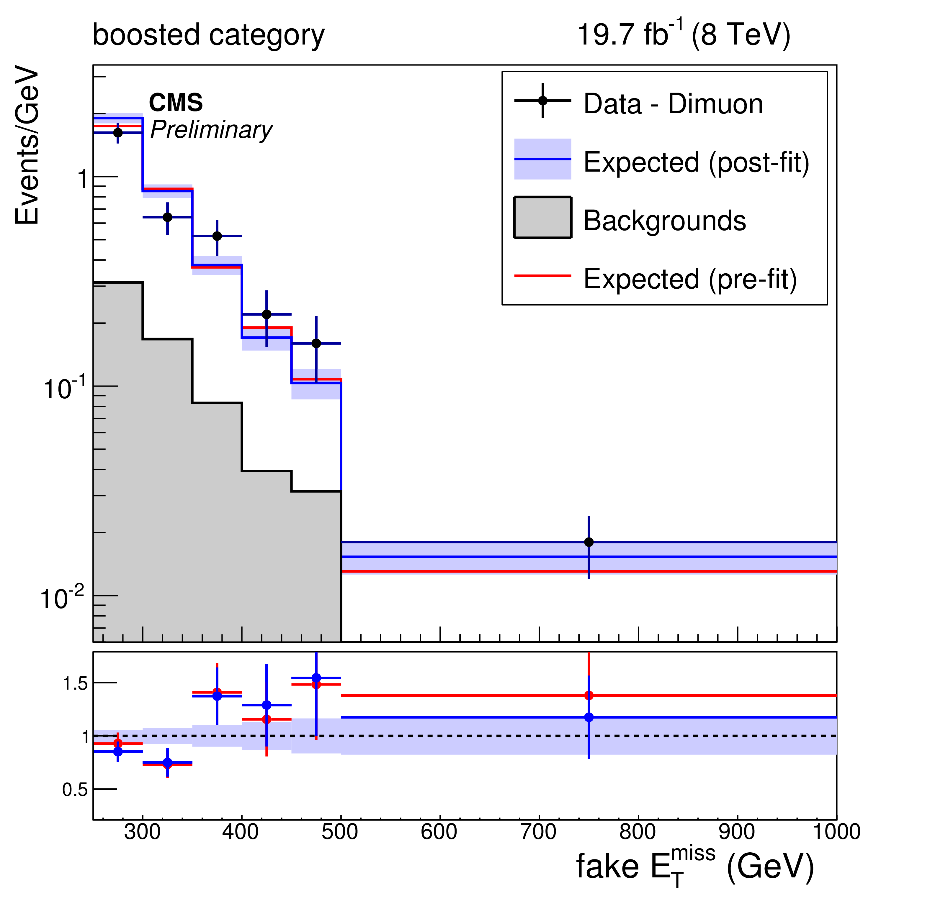
Figure 6-h:
Expected and observed fake $ {E_{\mathrm {T}}^{\text {miss}}} $ distributions in the photon(a,d,g), dimuon (b,e,h) and single-muon(c,f,i) control regions after performing the simultaneous likelihood fit to the control regions. Each series of plot, (a,b,c), (d,e,f) and (g,h,i), shows the result of the fit in the monojet, resolved and boosted event categories respectively. The red line represents the expected distribution before fitting to the control regions, while the blue line shows the expectation after the fit. In the ratio, the blue and red points show the ratio of the observed data to the post-fit and pre-fit expectations respectively. The blue bands indicate the statistical and systematic uncertainties from the fit. |

png ; pdf |
Figure 6-i:
Expected and observed fake $ {E_{\mathrm {T}}^{\text {miss}}} $ distributions in the photon(a,d,g), dimuon (b,e,h) and single-muon(c,f,i) control regions after performing the simultaneous likelihood fit to the control regions. Each series of plot, (a,b,c), (d,e,f) and (g,h,i), shows the result of the fit in the monojet, resolved and boosted event categories respectively. The red line represents the expected distribution before fitting to the control regions, while the blue line shows the expectation after the fit. In the ratio, the blue and red points show the ratio of the observed data to the post-fit and pre-fit expectations respectively. The blue bands indicate the statistical and systematic uncertainties from the fit. |
png ; pdf |
Figure 7-a:
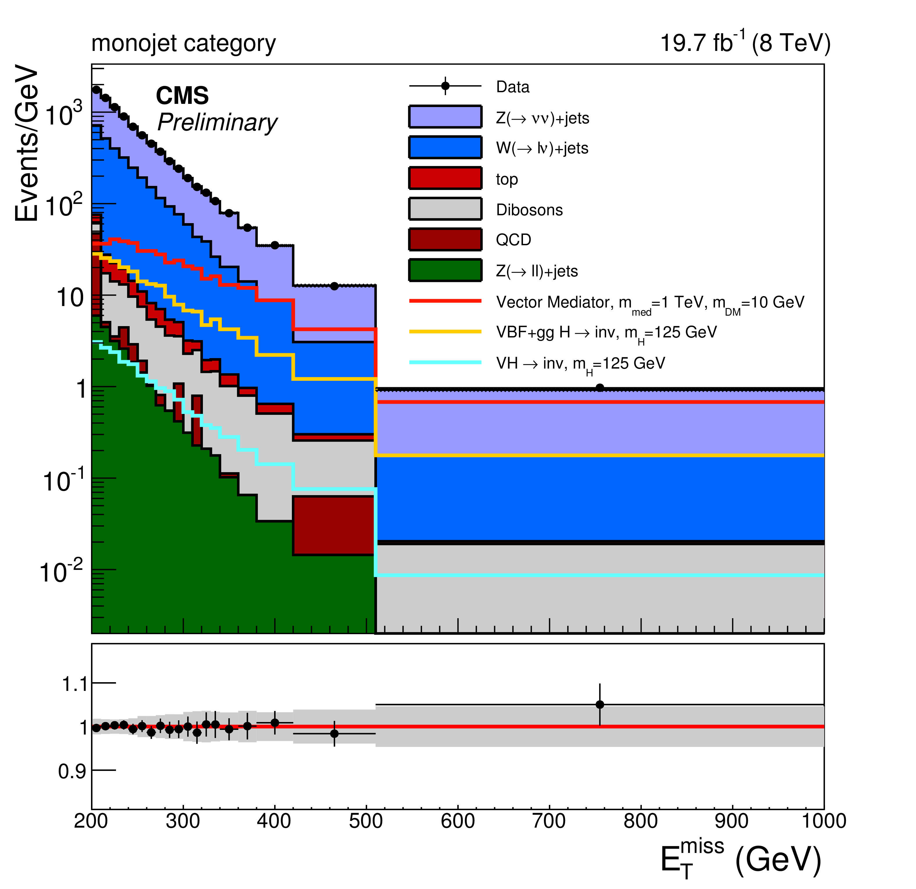
Post-fit distributions of $ {E_{\mathrm {T}}^{\text {miss}}} $ expected from SM backgrounds and observed in data in the signal region. The expected distributions are evaluated after fitting to the observed data simultaneously across the monojet (a), resolved (b) and boosted (c) categories. The gray bands indicate the post-fit uncertainty on the background, assuming no signal. The expected distribution from a Higgs boson with mass 125 GeV is shown, assuming a 100% branching ratio to invisible particles, split into the contributions from vector boson fusion and gluon fusion (VBF+ggH) and associated vector boson production modes (VH). |
png ; pdf |
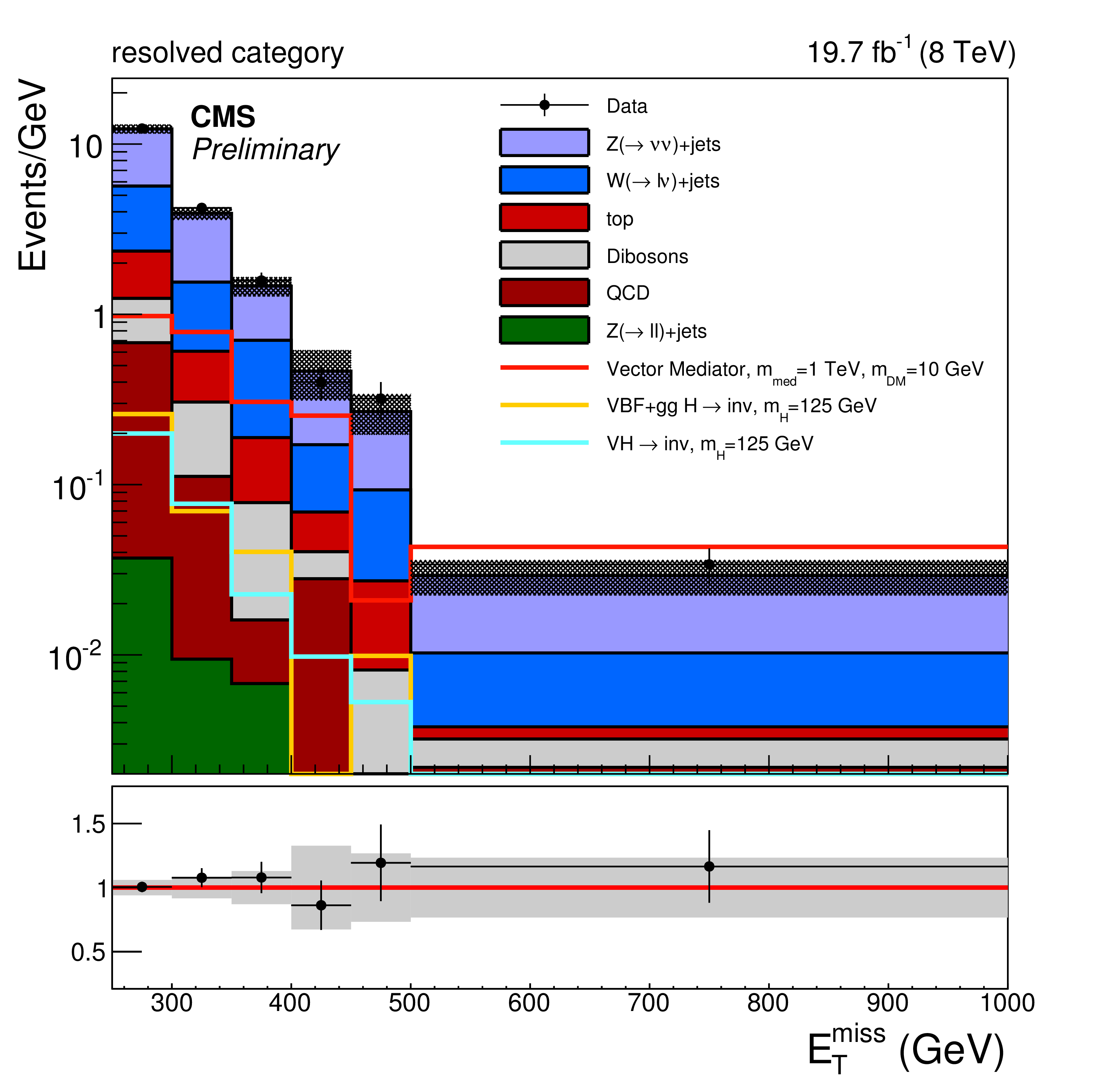
Figure 7-b:
Post-fit distributions of $ {E_{\mathrm {T}}^{\text {miss}}} $ expected from SM backgrounds and observed in data in the signal region. The expected distributions are evaluated after fitting to the observed data simultaneously across the monojet (a), resolved (b) and boosted (c) categories. The gray bands indicate the post-fit uncertainty on the background, assuming no signal. The expected distribution from a Higgs boson with mass 125 GeV is shown, assuming a 100% branching ratio to invisible particles, split into the contributions from vector boson fusion and gluon fusion (VBF+ggH) and associated vector boson production modes (VH). |
png ; pdf |
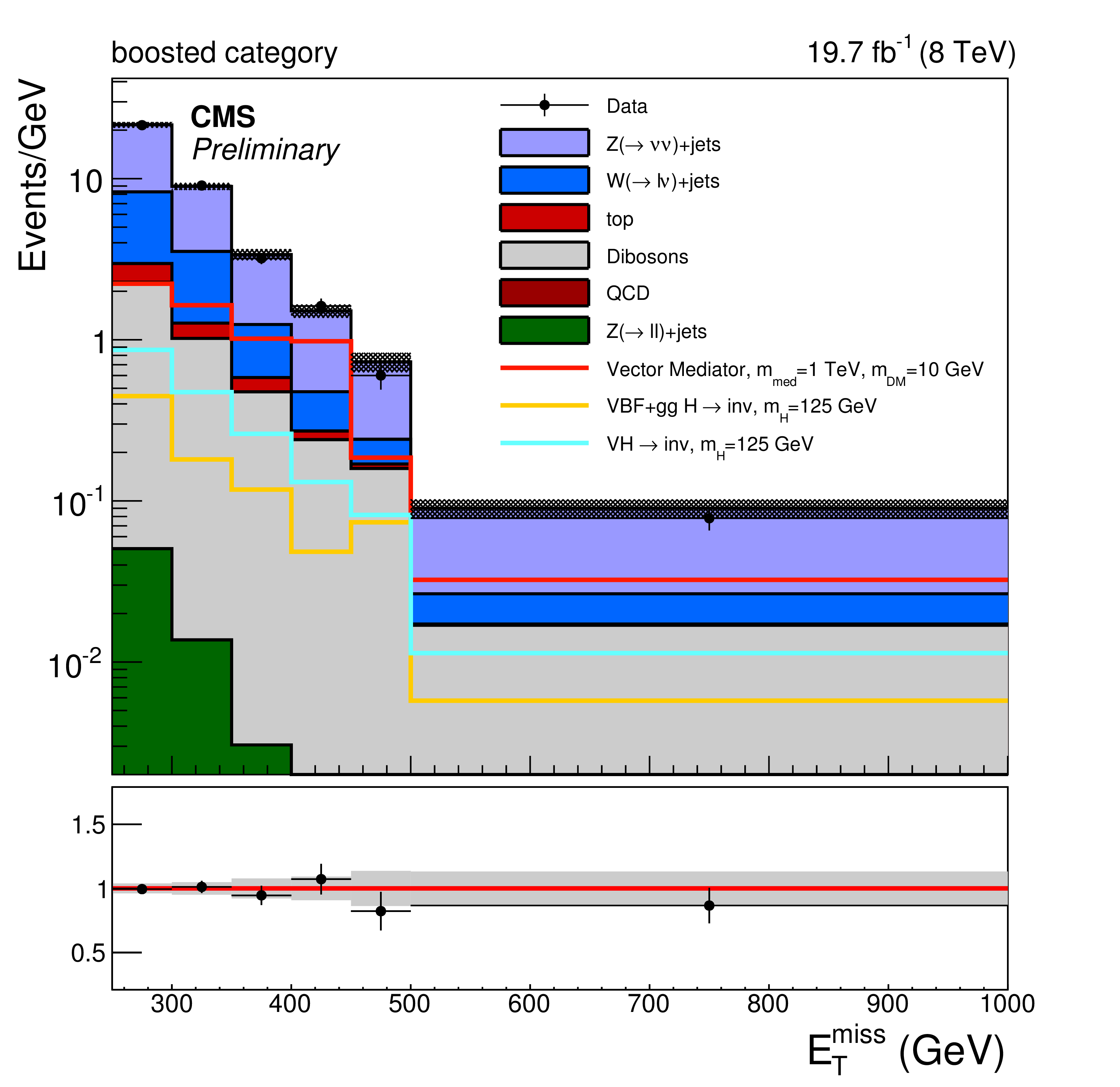
Figure 7-c:
Post-fit distributions of $ {E_{\mathrm {T}}^{\text {miss}}} $ expected from SM backgrounds and observed in data in the signal region. The expected distributions are evaluated after fitting to the observed data simultaneously across the monojet (a), resolved (b) and boosted (c) categories. The gray bands indicate the post-fit uncertainty on the background, assuming no signal. The expected distribution from a Higgs boson with mass 125 GeV is shown, assuming a 100% branching ratio to invisible particles, split into the contributions from vector boson fusion and gluon fusion (VBF+ggH) and associated vector boson production modes (VH). |
png ; pdf |
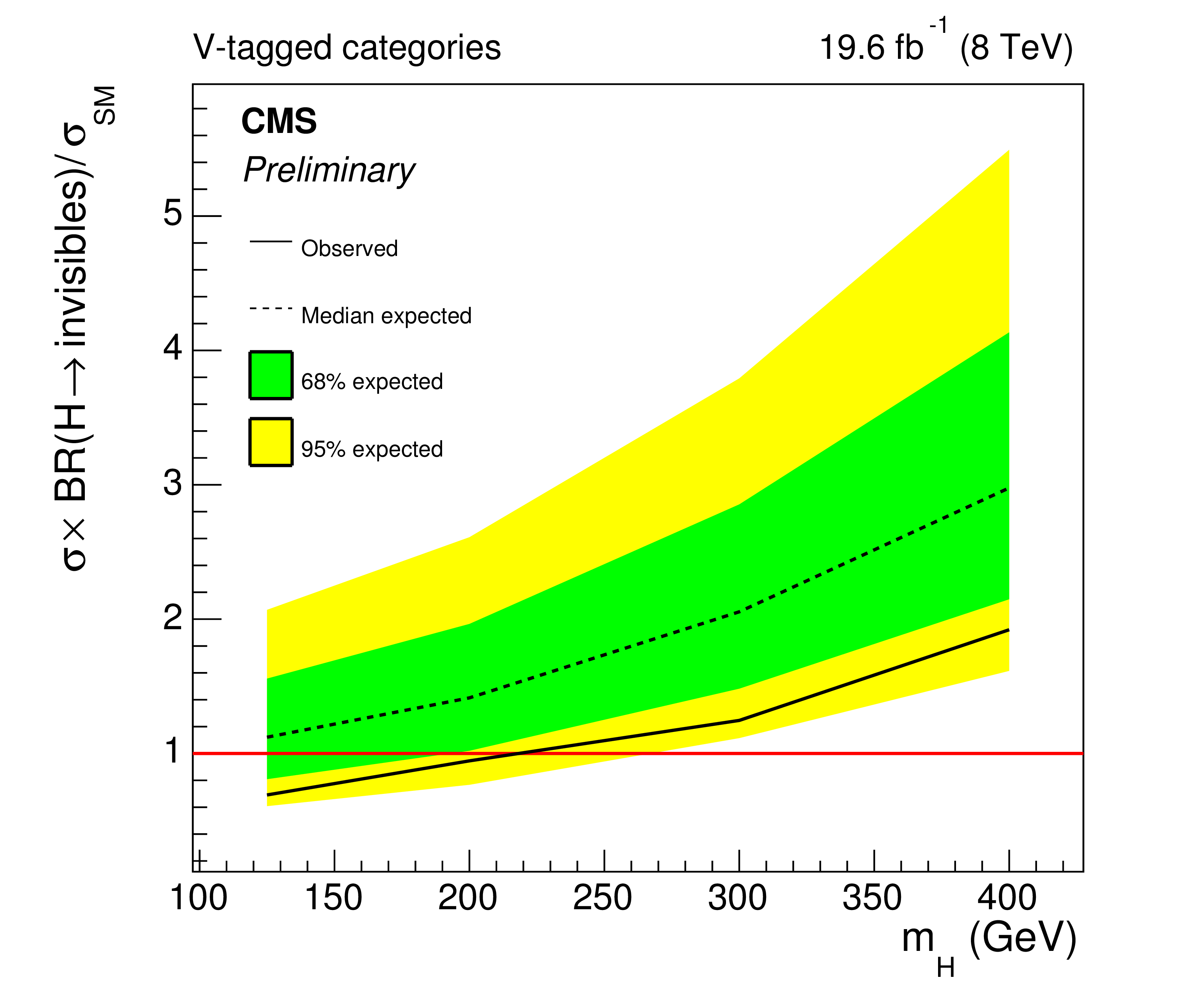
Figure 8-a:
Expected (dashed) and observed (solid) upper limits on $\mu $ at the 95% CL as a function of the Higgs boson mass when combining the two V-tagged categories (a) and combining all three categories (b) . |

png ; pdf |
Figure 8-b:
Expected (dashed) and observed (solid) upper limits on $\mu $ at the 95% CL as a function of the Higgs boson mass when combining the two V-tagged categories (a) and combining all three categories (b) . |

png ; pdf |
Figure 9-a:
90% CL Exclusion contours in the $m_{\textrm {med}}-m_{\textrm {DM}}$ plane assuming a vector (a), axial-vector (b), scalar (c), or pseudoscalar (d) mediator. The blue scale shows the 90% CL upper limit on the signal strength assuming the mediator only couples to fermions. For the scalar and pseudoscalar mediators, the exclusion contour assuming coupling only to fermions is explicitly shown in the orange line. The white region shows model points which were not tested when assuming coupling only to fermions and are not expected to be excluded by this analysis under this assumption. The excluded region is to the bottom-left of the contours shown in all cases except for that from the relic density as indicated by the shading. In all of the mediator models, a minimum width is assumed. |

png ; pdf |
Figure 9-b:
90% CL Exclusion contours in the $m_{\textrm {med}}-m_{\textrm {DM}}$ plane assuming a vector (a), axial-vector (b), scalar (c), or pseudoscalar (d) mediator. The blue scale shows the 90% CL upper limit on the signal strength assuming the mediator only couples to fermions. For the scalar and pseudoscalar mediators, the exclusion contour assuming coupling only to fermions is explicitly shown in the orange line. The white region shows model points which were not tested when assuming coupling only to fermions and are not expected to be excluded by this analysis under this assumption. The excluded region is to the bottom-left of the contours shown in all cases except for that from the relic density as indicated by the shading. In all of the mediator models, a minimum width is assumed. |

png ; pdf |
Figure 9-c:
90% CL Exclusion contours in the $m_{\textrm {med}}-m_{\textrm {DM}}$ plane assuming a vector (a), axial-vector (b), scalar (c), or pseudoscalar (d) mediator. The blue scale shows the 90% CL upper limit on the signal strength assuming the mediator only couples to fermions. For the scalar and pseudoscalar mediators, the exclusion contour assuming coupling only to fermions is explicitly shown in the orange line. The white region shows model points which were not tested when assuming coupling only to fermions and are not expected to be excluded by this analysis under this assumption. The excluded region is to the bottom-left of the contours shown in all cases except for that from the relic density as indicated by the shading. In all of the mediator models, a minimum width is assumed. |
png ; pdf |
Figure 9-d:
90% CL Exclusion contours in the $m_{\textrm {med}}-m_{\textrm {DM}}$ plane assuming a vector (a), axial-vector (b), scalar (c), or pseudoscalar (d) mediator. The blue scale shows the 90% CL upper limit on the signal strength assuming the mediator only couples to fermions. For the scalar and pseudoscalar mediators, the exclusion contour assuming coupling only to fermions is explicitly shown in the orange line. The white region shows model points which were not tested when assuming coupling only to fermions and are not expected to be excluded by this analysis under this assumption. The excluded region is to the bottom-left of the contours shown in all cases except for that from the relic density as indicated by the shading. In all of the mediator models, a minimum width is assumed. |
png ; pdf |
Figure 10-a:
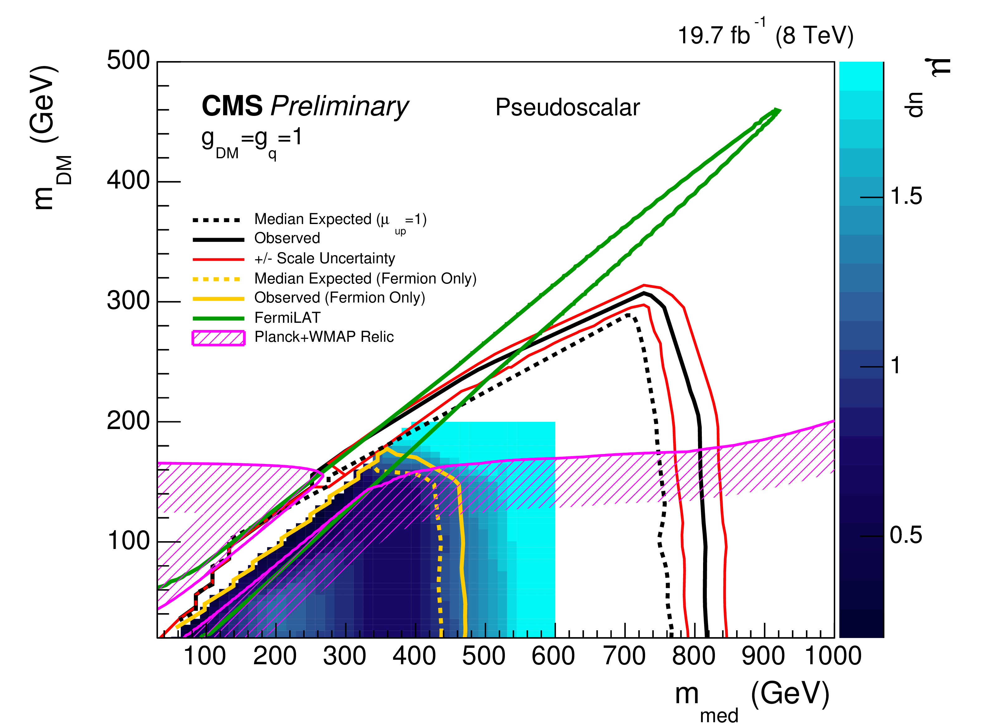
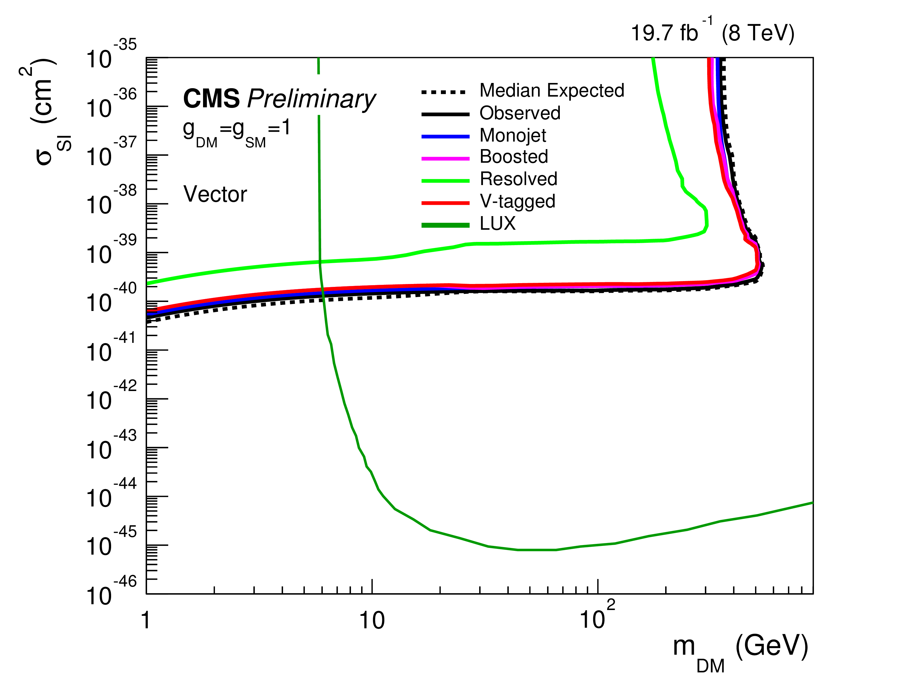
90% CL Exclusion contours in the $m_{\textrm {DM}}-\sigma _{\textrm {DM}}$ plane assuming a vector (a), axial-vector (b), scalar (c), or pseudoscalar (d) mediator. For the scalar and pseudoscalar case, the orange line shows the exclusion contours assuming the mediator only couples to fermions. The excluded region in all plots is to the top left of the contours shown. In the vector and axial-vector scenarios, limits are shown independently for monojet, boosted and resolved categories. The partial combination of the "V-tagged" categories (resolved and boosted) categories is shown for which the boosted category provides the dominant contribution. In all of the mediator models, a minimum width is assumed. For the pseudo-scalar, 68% CL preferred regions, using data from FermiLAT, for DM annihilation to light-quarks (qq), tau pairs ($\tau \tau $) and bottom-quark pairs (bb) are shown by the solid green, pink and brown coloured regions respectively. |

png ; pdf |
Figure 10-b:
90% CL Exclusion contours in the $m_{\textrm {DM}}-\sigma _{\textrm {DM}}$ plane assuming a vector (a), axial-vector (b), scalar (c), or pseudoscalar (d) mediator. For the scalar and pseudoscalar case, the orange line shows the exclusion contours assuming the mediator only couples to fermions. The excluded region in all plots is to the top left of the contours shown. In the vector and axial-vector scenarios, limits are shown independently for monojet, boosted and resolved categories. The partial combination of the "V-tagged" categories (resolved and boosted) categories is shown for which the boosted category provides the dominant contribution. In all of the mediator models, a minimum width is assumed. For the pseudo-scalar, 68% CL preferred regions, using data from FermiLAT, for DM annihilation to light-quarks (qq), tau pairs ($\tau \tau $) and bottom-quark pairs (bb) are shown by the solid green, pink and brown coloured regions respectively. |

png ; pdf |
Figure 10-c:
90% CL Exclusion contours in the $m_{\textrm {DM}}-\sigma _{\textrm {DM}}$ plane assuming a vector (a), axial-vector (b), scalar (c), or pseudoscalar (d) mediator. For the scalar and pseudoscalar case, the orange line shows the exclusion contours assuming the mediator only couples to fermions. The excluded region in all plots is to the top left of the contours shown. In the vector and axial-vector scenarios, limits are shown independently for monojet, boosted and resolved categories. The partial combination of the "V-tagged" categories (resolved and boosted) categories is shown for which the boosted category provides the dominant contribution. In all of the mediator models, a minimum width is assumed. For the pseudo-scalar, 68% CL preferred regions, using data from FermiLAT, for DM annihilation to light-quarks (qq), tau pairs ($\tau \tau $) and bottom-quark pairs (bb) are shown by the solid green, pink and brown coloured regions respectively. |

png ; pdf |
Figure 10-d:
90% CL Exclusion contours in the $m_{\textrm {DM}}-\sigma _{\textrm {DM}}$ plane assuming a vector (a), axial-vector (b), scalar (c), or pseudoscalar (d) mediator. For the scalar and pseudoscalar case, the orange line shows the exclusion contours assuming the mediator only couples to fermions. The excluded region in all plots is to the top left of the contours shown. In the vector and axial-vector scenarios, limits are shown independently for monojet, boosted and resolved categories. The partial combination of the "V-tagged" categories (resolved and boosted) categories is shown for which the boosted category provides the dominant contribution. In all of the mediator models, a minimum width is assumed. For the pseudo-scalar, 68% CL preferred regions, using data from FermiLAT, for DM annihilation to light-quarks (qq), tau pairs ($\tau \tau $) and bottom-quark pairs (bb) are shown by the solid green, pink and brown coloured regions respectively. |
| Tables | |

png ; pdf |
Table 1:
Systematic uncertainties and their relative effect on the expectation for the SM backgrounds. |
png ; pdf |
Table 2:
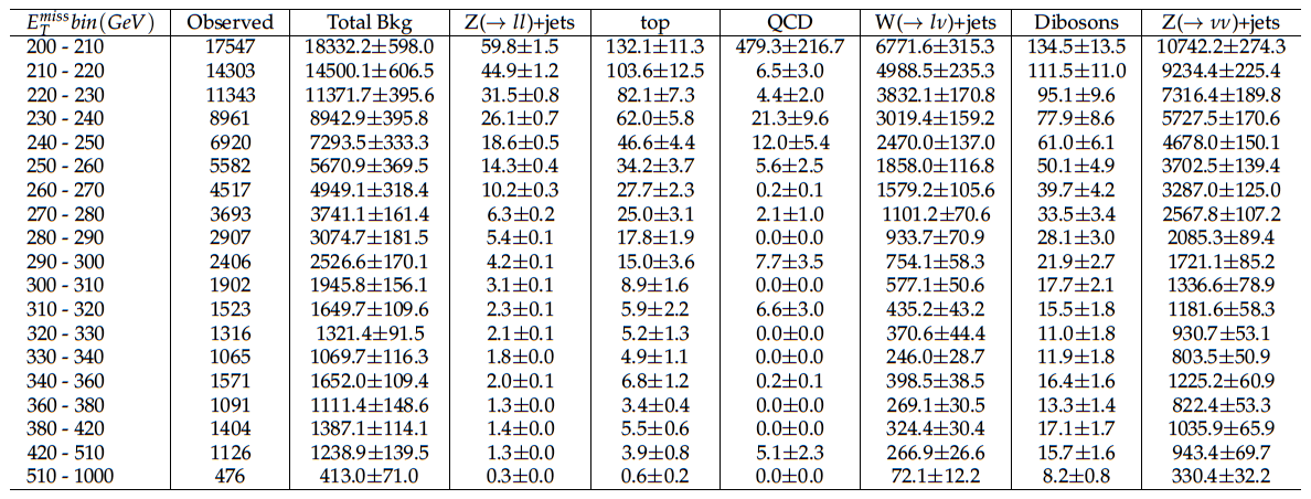
Expected yields of the standard model processes and their uncertainties per bin for the monojet category signal region after applying all corrections to the MC. |

png ; pdf |
Table 3:
Expected yields of the standard model processes and their uncertainties per bin for the resolved category signal region after applying all corrections to the MC. |

png ; pdf |
Table 4:
Expected yields of the standard model processes and their uncertainties per bin for the boosted category signal region after applying all corrections to the MC. |
| Summary |
| A search has been presented for an excess of events with a high energy jet in association with a large missing transverse momentum in a data sample of proton-proton interactions at centre of mass energy of 8 TeV. The data correspond to an integrated luminosity of 19.7 fb$^{-1}$ collected by the CMS detector at the LHC. Sensitivity to mono-V models is achieved by tagging events consistent with the jet originating from a hadronically decaying vector boson. No significant deviation from the expectation from SM backgrounds is observed in the $E_{\mathrm{T}}^{\text{miss}} $ distributions. A 95% CL observed (expected) upper limit of 0.53 (0.62) is obtained on the branching ratio of a SM Higgs boson with a mass of 125 GeV decaying to invisible particles. The search is also interpreted in terms of DM production to place constraints on the parameter space of the simplified models considered. From these, constraints are placed on dark-matter-nucleon scattering cross-sections using both spin-dependent and spin-independent interactions. |
|
|
Compact Muon Solenoid LHC, CERN |
|

|

|

|

|

|